inequality and aggregate demand - usc dana and … and aggregate demand adrien auclert matthew...

Inequality and Aggregate Demand

Adrien Auclert Matthew Rognlie

Stanford Northwestern

USC/INETConference on Inequality, Globalization, and Macroeconomics

April 28, 2017

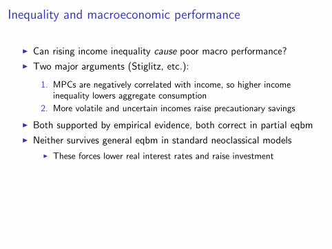
Inequality and macroeconomic performance

I Can rising income inequality cause poor macro performance?

I Two major arguments (Stiglitz, etc.):

1. MPCs are negatively correlated with income, so higher incomeinequality lowers aggregate consumption

2. More volatile and uncertain incomes raise precautionary savings

I Both supported by empirical evidence, both correct in partial eqbm

I Neither survives general eqbm in standard neoclassical models

I These forces lower real interest rates and raise investment

I We show that inequality lowers output at the zero lower bound

I Quantify the potential effect of 1 & 2I Investment usually falls (’paradox of thrift’)I Depressed economy even in long run (’secular stagnation’)

What we do

I Take canonical Huggett-Aiyagari modelI Add downward nominal wage ridigidites (DNWR)I Parsimonious, allows focus on household demand

I Calibrate to 2013 U.S.I Binding zero lower bound (ZLB): r = π = i = 0%I Mildly depressed employment: L < 1

I Main questn: what happens if inequality unexpectedly rises further?

I Temporarily (income redistribution)I Permanently (change in income process)

under various assumptions about fiscal policyI Key: binding ZLB + DNWR

I ⇒ most of eqbm adjustment happens via unemploymentI In particular steady state r fixed, L adjusts to clear markets

Contributions

I Foundation for the transmission mechanism of inequality to outputvia an ’aggregate demand channel’

I Key forces in general equilibrium:

I Inequality multiplier from endogenous inequality changeI Paradox of thrift due to effect of L on MPKI Importance of government spending and public debt policy

I Novel two-step approach to quantifying magnitudes:

Output effect = (GE multiplier) · (PE sufficient statistic)

I Sufficient statistics are measurable:

I Short run: Cov(MPC , dy

Y

)I Long run: elasticity of savings to idiosyncratic risk

I Multiplier characterizes the response to any aggregate demand shock

I Depends only on model parameters and policy

Related literature

I Incomplete markets, inequality, and aggregate savings

I Aiyagari (1994), Krusell-Smith (1998), Heathcote-Storesletten-Violante(2010), Krueger-Mitman-Perri (2015), Kuhmhof-Ranciere-Winant (2015)

I Interaction with nominal rigidities

I Guerrieri-Lorenzoni (2015), Oh-Reis (2013), McKay-Reis (2016)I Gornemann, Kuester and Nakajima (2014), Sheedy (2014), McKay,

Nakamura and Steinsson (2015), Auclert (2016), Werning (2015), Kaplan,Moll and Violante (2016), Bilbiie-Ragot (2016)

I Ravn-Sterk (2013), den Haan, Rendahl and Riegler (2014), Bayer et al(2014), Challe-Matheron-Ragot-Rubio (2015), Heathcote-Perri (2016)

I Secular stagnation

I Eggertsson-Mehrotra (2014), Caballero-Farhi-Gourinchas (2016),Benigno-Fornaro (2016), Eggertsson, Mehrotra, Singh and Summers (2016)

I Public debt, liquidity, and safe assets

I Woodford (1990), Aiyagari-McGrattan (1998), Caballero-Farhi (2015)

I Sufficient statistics approaches in macro

I Shimer-Werning (2009), Auclert (2016), Berger et al (2015)

Outline

1. Model overview and calibration

2. Temporary increase in income inequality

3. Permanent increase in income inequality

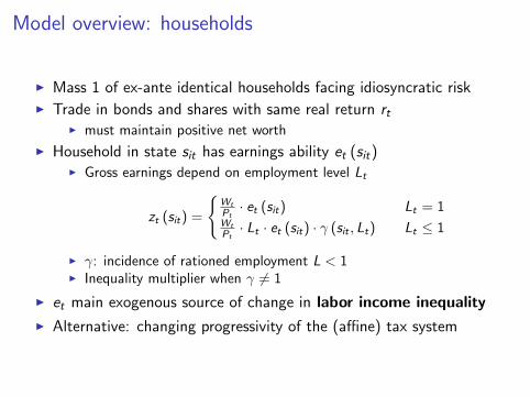
Model overview: households

I Mass 1 of ex-ante identical households facing idiosyncratic riskI Trade in bonds and shares with same real return rt

I must maintain positive net worth

I Household in state sit has earnings ability et (sit)I Gross earnings depend on employment level Lt

zt (sit) =

{Wt

Pt· et (sit) Lt = 1

Wt

Pt· Lt · et (sit) · γ (sit , Lt) Lt ≤ 1

I γ: incidence of rationed employment L < 1I Inequality multiplier when γ 6= 1

I et main exogenous source of change in labor income inequality

I Alternative: changing progressivity of the (affine) tax system

Firms and the labor and capital markets

I Firms produce a final good (price Pt)I Production function Ft (Kt−1, Lt) (constant returns)I Exogenous markup µt (⇒ monopoly profits)I Always on labor demand curve

FLt (Kt−1, Lt) = µtWt

Pt

I Capital investment determined by Q theory

I Dw. wage rigidities: impose Wt ≥Wt−1, when binding Lt < 1

I Labor share changes (µt , Ft) alternative source of inequality

Government policy and equilibrium

I Fiscal authority: has fiscal rules for Gt and deficits, ensuring

τtWt

PtLt + Bt = Gt + (1 + rt−1) Bt−1

In benchmark: Gt = G and Bt = B at all t. Other rules

I Central bank sets nominal interest rate it st ZLB & 0 infl. target

1 + it = max

{1, (1 + rnt )

(Pt

Pt−1

)φ}

φ > 1 (Taylor principle); rnt is real rate without nominal frictionsI Equilibrium definition standard go uniqueness

Calibration: steady state

Parameters Description Main calibration Target

(e, S,Λ) Income process KMV (2016) W2 moments

γ Incidence function 1 Equal incidence

ν EIS 0.5 Standard calibration

β Discount factor 0.964 r = 0

ε K − L elasticity 1 Standard calibration

δ Depreciation rate 4.4% NIPA 2013

i Nominal interest rate 0% ZLB

r Eqbm real rate 0% TIPS yields 2013

L Employment gap 0.97 CBO output gap estimate

ξ Wage deflation rate 1 1+i1+r

KY

Capital-output ratio 330% FoF hh. net worth 2013

θ(a) Initial asset allocation SCF 2013

µ Monopoly markup 1

BY

Govt debt 59.0% Domestic holdings 2013

GY

Govt spending rate 18.7% NIPA 2013

τr Tax redistribution 17.5 CBO (2016)

Labor income inequality trends

1980 1990 2000 2010

0.8

0.84

0.88

0.92

Year

Log

poi

nts

US income inequality and the real interest rate

Standard dev. of log gross earningsModel calibration

0

1

2

3

4

Per

cen

t

Laubach-Williams r?

Model calibration

Source: Song, Price, Guvenen, Bloom and von Wachter (2016)

; Laubach and Williams (2015)

Labor income inequality trends

1980 1990 2000 2010

0.8

0.84

0.88

0.92

Year

Log

poi

nts

US income inequality and the real interest rate

Standard dev. of log gross earningsModel calibration

0

1

2

3

4

Per

cen

t

Laubach-Williams r?

Model calibration

Source: Song, Price, Guvenen, Bloom and von Wachter (2016); Laubach and Williams (2015)

Outline




0 10 20 30 40 50

−0.1

−0.05

0

Per

cent

0 10 20 30 40 50−0.2

−0.15

−0.1

−0.05

0

0 10 20 30 40 50

−2

−1

0·10−2

0 10 20 30 40 50−0.6

−0.4

−0.2

0

0 10 20 30 40 50−0.15

−0.1

−0.05

0

Years

Per

cent

0 10 20 30 40 50

−8

−6

−4

−2

0·10−3

Years0 10 20 30 40 50

00.5

11.5

2

·10−2

Years

ZLB

0 10 20 30 40 500.92

0.93

0.93

0.94

0.94

Years

Output Consumption Investment Real rate (bps)

Labor Capital Real wage sd log earnings (level)

0 10 20 30 40 50

−0.1

−0.05

0

Per

cent

0 10 20 30 40 50−0.2

−0.15

−0.1

−0.05

0

0 10 20 30 40 50

0

0.1

0.2

0.3

0.4

0 10 20 30 40 50−4

−3

−2

−1

0

0 10 20 30 40 50−0.15

−0.1

−0.05

0

Years

Per

cent

0 10 20 30 40 50

0

2

4

·10−2

Years0 10 20 30 40 50

00.5

11.5

2

·10−2

Years

ZLB No-ZLB

0 10 20 30 40 500.92

0.93

0.93

0.94

0.94

Years



0 10 20 30 40 50−0.15

−0.1

−0.05

0

Per

cent

0 10 20 30 40 50−0.2

−0.15

−0.1

−0.05

0

0 10 20 30 40 50−0.1

00.10.20.30.4

0 10 20 30 40 50−4

−3

−2

−1

0

0 10 20 30 40 50

−0.15

−0.1

−0.05

0

Years

Per

cent

0 10 20 30 40 50−2

0

2

4

·10−2

Years0 10 20 30 40 50

0

1

2

·10−2

Years

ZLB No-ZLB Constant r

0 10 20 30 40 500.92

0.93

0.93

0.94

0.94

Years



Understanding and decomposing the effect

I Consider general perturbation to after-tax incomes dyi0 st E [dyi0] = 0

I In partial equilibrium (rt , Lt fixed): change in Ct path

∂Ct = CovI (MPCit , dyi0)

where MPCit = is i ’s spending at t of date-0 income

I One shock, one sufficient statistic

I In general equibriumdY = G · ∂C

G is GE matrix, independent of source of demand shock

I ∂C can be evaluated with micro dataI G easily solved for numericallyI in our calibration, loads on ∂C0 and is close to 1 Show

0 20 40 60−0.1

−0.08

−0.06

−0.04

−0.02

0P

erce

nt

0 20 40 60

0

0.5

1

Lev

el

BenchmarkΓ = −0.15

0 20 40 60

−0.1

−0.05

0

Years

Per

cen

t

Actual path dY /Y

Predicted G · ∂C/Y

0 5 10 15 20−0.15

−0.1

−0.05

0

Years

BenchmarkΓ = −0.15

PE consumption response ∂C/Y GE multipliers for date 0 output G0

GE output response dY /Y dY /Y with varying Γ

Back

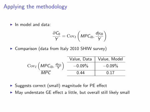
Applying the methodology

I In model and data:

∂C0

Y= CovI

(MPCi0,

dyi0Y

)I Comparison (data from Italy 2010 SHIW survey)

Value, Data Value, Model

CovI

(MPCi0,

dyi0Y

)−0.09% −0.09%

MPC 0.44 0.17

I Suggests correct (small) magnitude for PE effect

I May understate GE effect a little, but overall still likely small

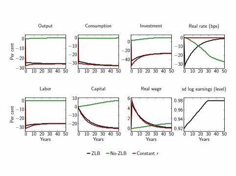
Outline




0 10 20 30 40 50

−20

−10

0

Per

cent

0 10 20 30 40 50

−30

−20

−10

0

0 10 20 30 40 50

−40

−30

−20

−100

0 10 20 30 40 50

−30

−20

−10

0

0 10 20 30 40 50−30

−20

−10

0

Years

Per

cent

0 10 20 30 40 50

−20

−10

0

Years0 10 20 30 40 50

012345

Years

ZLB

0 10 20 30 40 500.92

0.94

0.96

0.98

Years



0 10 20 30 40 50

−20

−10

0

Per

cent

0 10 20 30 40 50

−30

−20

−10

0

0 10 20 30 40 50

−40

−20

0

0 10 20 30 40 50

−30

−20

−10

0

0 10 20 30 40 50−30

−20

−10

0

Years

Per

cent

0 10 20 30 40 50

−20

−10

0

10

Years0 10 20 30 40 50

012345

Years

ZLB No-ZLB

0 10 20 30 40 500.92

0.94

0.96

0.98

Years



0 10 20 30 40 50−30

−20

−10

0

Per

cent

0 10 20 30 40 50

−30

−20

−10

0

0 10 20 30 40 50

−40

−20

0

0 10 20 30 40 50

−30

−20

−10

0

0 10 20 30 40 50

−30

−20

−10

0

Years

Per

cent

0 10 20 30 40 50

−20

−10

0

10

Years0 10 20 30 40 50

0

2

4

6

Years

ZLB No-ZLB Constant r

0 10 20 30 40 500.92

0.94

0.96

0.98

Years



0 10 20 30 40 50

−20

−10

0

Per

cent

0 10 20 30 40 50

−30

−20

−10

0

0 10 20 30 40 50

−40

−30

−20

−100

0 10 20 30 40 50

−30

−20

−10

0

0 10 20 30 40 50−30

−20

−10

0

Per

cent

0 10 20 30 40 50

−20

−10

0

0 10 20 30 40 50012345

0 10 20 30 40 500.92

0.94

0.96

0.98

0 10 20 30 40 50

−0.5

0

0.5

1

Years

Per

cent

0 10 20 30 40 50

−0.5

0

0.5

1

Years0 10 20 30 40 50

22

24

26

28

30

Years

Benchmark ZLB



Govt spending Govt debt Tax rate

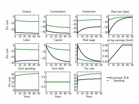
0 10 20 30 40 50

−20

−10

0

Per

cent

0 10 20 30 40 50

−30

−20

−10

0

0 10 20 30 40 50

−40

−30

−20

−100

0 10 20 30 40 50

−30

−20

−10

0

0 10 20 30 40 50−30

−20

−10

0

Per

cent

0 10 20 30 40 50

−20

−10

0

0 10 20 30 40 50012345

0 10 20 30 40 500.92

0.94

0.96

0.98

0 10 20 30 40 500

10

20

30

40

Years

Per

cent

0 10 20 30 40 50

−0.5

0

0.5

1

Years0 10 20 30 40 50

222426283032

Years

Benchmark ZLBSpending




0 10 20 30 40 50

−20

−10

0

Per

cent

0 10 20 30 40 50

−30

−20

−10

0

0 10 20 30 40 50

−40

−30

−20

−100

0 10 20 30 40 50

−30

−20

−10

0

0 10 20 30 40 50−30

−20

−10

0

Per

cent

0 10 20 30 40 50

−20

−10

0

0 10 20 30 40 50012345

0 10 20 30 40 500.92

0.94

0.96

0.98

0 10 20 30 40 500

10

20

30

40

Years

Per

cent

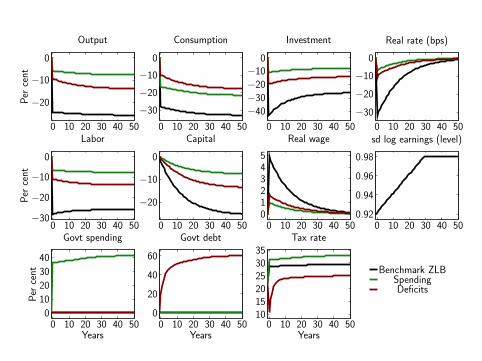
0 10 20 30 40 500

20

40

60

Years0 10 20 30 40 50

101520253035

Years

Benchmark ZLBSpendingDeficits




Understanding the effect: steady state

I Assume Γ = 0 (no ineq. multiplier)

I Experiment: steady-state comp statics wrt index of inequality σ

I Asset market clearing

A

(r , σ, τ,

W

P, L

)= B + K

I Homotheticity + govt budget constraint + factor demands(w (r) L−

(G + rB

))a (r , σ) = B + κ (r) L

Equilibrium: (A, L) space(w (r) L−

(G + rB

))a (r , σ) = B + (κ (r) + π (r)) L

Asset Supply

Asset Demand

L

A = B + K

L

B

G+rBw(r)

Government multipliers Multiple SS with Γ < 0

Equilibrium: (A, L) space(w (r) L−

(G + rB

))a (r , σ) = B + (κ (r) + π (r)) L

L

A = B + K

L

B

G+rBw(r)

Government multipliers Multiple SS with Γ < 0

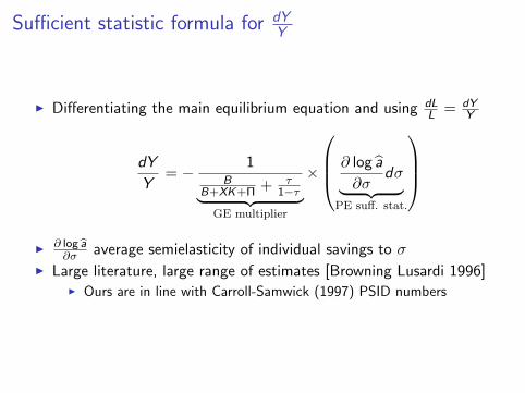
Sufficient statistic formula for dYY

I Differentiating the main equilibrium equation and using dLL = dY

Y

dY

Y= − 1

BB+XK+Π + τ

1−τ︸︷︷︸GE multiplier

×

∂ log a

∂σdσ︸︷︷︸

PE suff. stat.

I ∂ log a

∂σ average semielasticity of individual savings to σI Large literature, large range of estimates [Browning Lusardi 1996]

I Ours are in line with Carroll-Samwick (1997) PSID numbers

Extensions

1. Change in capital-labor distribution:

I Decline in labor share from relative price of investment(Piketty/Karabarbounis-Neiman)

I Monopoly profits: µt (Summers/Krugman)

2. Inequality and the r∗ decline Go

3. Government spending and liquidity multipliers Go

Conclusion

I Canonical macro model of inequality + nominal wage rigiditiesI Allows to study effect of aggregate demand shocks on output,

including inequalityI Very tractable and flexible, codes online soon

I Theory highlights importance of empirical evidence on

I MPC heterogeneity [Cov (MPC , y)] (short-run)I Effect of income uncertainty on savings [∂ log A

∂σ ] (long-run)I Distributional incidence of recessions [Γ] (both)

I Amplification role of private investment

I Stabilizing role of monetary (r) and fiscal policy (G and B)

Thank you!

Fiscal rule

I Fiscal rules are for government spending and target deficits

Gt = G (Lt) Dt = D (Lt)

Ensure debt sustainability by setting τt such that

τtWt

PtLt =

(G (Lt) + rt−1Bt−1 − D (Lt)

)︸︷︷︸Target taxes

(Bt−1

Bss

)ετ,BI Implies elasticity of B to L of

εB,L =1

ετ,B

1

G ss + rBss eD,L =

1

1− ρ1

Bss eD,L

where eD,L is semielasticity of D to L and ρ is persistence of deficits

I Calibration: ρ = 0.5 andI “Deficits”: eD,L = −1, eG ,L = 0I “Spending”: eD,L = 0, eG ,L = −1

Back

Steady-state with ZLB has constant r

Proposition

Assume a unique neoclassical steady state with rn < 0. Then, in anysteady state of the model with rigidities & ZLB, i = 0 and Pt

Pt−1= ξ < 1

In particular, steady state r = 1ξ − 1 > 0 > rn

I Proof: in steady-state PtPt−1

= WtWt−1

= Π

I If Π > ξ, by complementary slackness L = 1, so r = rn < 0I Impossible by monetary policy rule:

I If ZLB does not bind, inflation target ⇒ Π = 1, so ZLB does bindI If ZLB binds, Π = 1

1+rn , so monetary policy raises i > 0

I Hence Π = ξ < 1, so (1 + rn) (Π)φ < 1, so ZLB binds

Corollary (Paradox of flexibility)

Lower ξ → higher r → lower L (typically)

Back

Equilibrium

I Given K−1, shocks {et , τ rt ,Xt , µt ,Ft} and initial joint distributionΨ0 (s, b, v), equilibrium is {Ct , It ,Yt ,Kt−1, Lt,dt ,Bt , τt},{rt , it ,Pt ,Wt , qt}, {ct (s, b, v) , bt (s, b, v) , vt (s, b, v)} andΨt (s, b, v) such that:

I Households and firms optimizeI Government follows fiscal and monetary policy rulesI Goods, bonds and capital markets clear

Ct + Xt It + Gt + Xtζ

(Kt − Kt−1

Kt−1

)Kt−1 = Yt = F (Kt−1, Lt)

Bt ≡ E [bit ] = B t

Vt ≡ E [vit ] = 1

Lt ≤ 1

Wt ≥Wt−1

(Lt − 1) (Wt −Wt−1) = 0

I Distributions evolve consistently with policy functions Back

Calibrating the retention function

I Model relationship between net income y and gross z :

yitE [zit ]

= (1− τ)

(τr + (1− τr )

zitE [zit ]

)I CBO data on avg transfers and taxes per nonelderly household by

income in 2006: overall AMI $95,000 and

Quintiles of market income Q1 Q2 Q3 Q4 Q5

Average market income (AMI) zit 12,600 36,100 59,500 89,900 240,800

AMI + Transfers minus taxes yit 25,200 36,300 51,400 72,700 174,800

I Yields yitE[zit ]

= 0.143 + 0.666 zitE[zit ]

with R2 = 0.9988

I Implying τ r = 0.1430.143+0.666

Back

Calibrating household portfoliosI Obtain θ (a) parametrically from SCF

I fraction invested in ’shares’ as function of total assets a = b + pvI broad definition: all net worth except deposits and bondsI narrow definition: only equity and shares

-8 -6 -4 -2 0 2 4

Log (net worth/average net worth)

0

0.1

0.2

0.3

0.4

0.5

0.6

0.7

0.8

0.9

1

Fra

ction o

f share

s in n

et w

ort

h θ

(a)

Micro-level distribution of capital holdings

SCF 2013: broad capital ownership

Fitted curve, θb(a)

SCF 2013: directly held equity

Fitted curve, θeq

(a)

Back

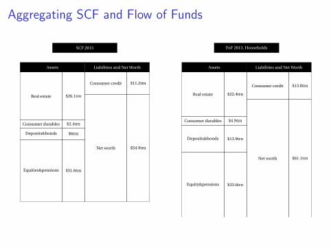
Aggregating SCF and Flow of Funds

SCF 2013

Assets Liabilities and Net Worth

FoF 2013, Households

Assets Liabilities and Net Worth

Real estate $26.1trn

Consumer durables $2.4trn

Deposits&bonds $6trn

Equities&pensions $31.6trn

Consumer credit $11.2trn

Net worth $54.9trn

Real estate $22.4trn

Consumer durables $4.9trn

Deposits&bonds $13.9trn

Equity&pensions $33.6trn


Net worth $61.1trn

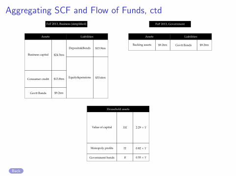
Aggregating SCF and Flow of Funds, ctdFoF 2013, Business (simplified)

Assets Liabilities

FoF 2013, Government

Assets Liabilities

Business capital $24.5trn


Govtt Bonds $9.2trn

Deposits&Bonds $13.9trn

Equity&pensions $33.6trn

Backing assets $9.2trn Govtt Bonds $9.2trn

Household assets

Value of capital XK 2.29 × Y

Monopoly profits Π 0.82 × Y

Government bonds B 0.55 × Y

Back

Calibration: steady state, with eq premium

Parameters Description Main calibration Target

ν EIS 0.5 Standard calibration

β Discount factor 0.972 r = 0

ε K − L elasticity 1 Standard calibration

α Labor share 62.5% NIPA 2013

δ Depreciation rate 5.6% NIPA 2013

r Eqbm real rate 0% TIPS yields 2013

µ Monopoly markup 1.067 ΠY

=1− 1

µ

r+%

% Equity premium 7.3%1µ−α

r+%+δ= K

Y

XKY

Capital-output ratio 229% BEA Fixed Assets 2013

ΠY

Capitalized profits 82.0% FoF hh. net worth 2013

BY

Govt debt 55.0% Domestic holdings 2013

IY

Investment rate 13.5% δ KY

GY

Govt spending rate 18.7% NIPA 2013

τ Headline tax rate 29.8% G+rBαY

r Keynesian policy rate 0% Zero lower bound

Back

Distribution summary statistics

Percentage held by Bottom/Top

sd. log Gini B 40% T 20% T 10% T 5% T 1%

ConsumptionModel 0.54 0.31 22% 41% 26% 16% 5%

Data 0.65 0.33 19% 40% 24% 14% 4%

Pretax IncomeModel 0.92 0.51 13% 52% 31% 26% 5%

Data 0.95 0.51 12% 55% 39% 28% 13%

WealthModel 2.22 0.79 1% 83% 66% 47% 17%

Data 2.22 0.81 1% 84% 72% 60% 33%

Back

Approximation to GE matrix G

I Obtain by assuming Lt = 1 for t ≥ 1:

I employment changes only today

I From investment problem: q0, I0 and p0 are constant

I Neoclassical theory determines changes in real wage and dividend as

d (d0) = d

(R0

P0

)K−1 =

1− αε

dY0 = −d

(W0

P0

)L0

I α ≡ labor share, ε ≡ elasticity of subst. bw capital and labor

I Individual i ’s consumption changes by

dci0 = MPCi0

{dyi0 + d

(yGEi0 − yi0

)+ vid (d0)

}I Direct effect of the redistributionI + effects from changing post-tax incomes and dividends

Approximation to GE matrix G, ctd

I Aggregate per capita consumption:

dC0 = E [dci0] = dY0 =W0

P0dL0

I Putting it all together:

dY0

Y0' 1

1− cΓ−(MPCy−MPC

v) 1−αε

1−MPCy︸︷︷︸

Inequality multiplier

× 1

1−MPCy︸︷︷︸

Keynesian multiplier

× Cov

(MPCi ,

dyiY0

)︸︷︷︸Redistributive impulse

I MPCy: income-weighted, MPC

v: share-weighted

I c = (1− τ)(1− τ r )Cov(

MPCi ,zi

E[zi ]log(

ziE[zi ]

))I Captures all static GE effects

I Misses dynamic feedbacks from future L to C and I

Back

Effects of G and B(w (r) L−

(G + rB

))a (r , ϕ) = B + κ (r) L

L

A = B + K

1

B

G+rBw(r)

G ′+rBw(r)

Effects of G and B(w (r) L−

(G + rB

))a (r , ϕ) = B + κ (r) L

L

A = B + K

1

B

G+rBw(r)

B′

Government multipliers and crowding-in

Proposition

While L < 1, steady-state output is given by

Y = αGG + αBB

where the government spending multiplier is

αG =1

α(

1− (1− τ) K+ΠB+K+Π

) > 1

and the government debt multiplier is

αB = αGC

A> 0

Back

Inequality multiplier and multiple steady states

0 1 2 3 40

0.2

0.4

0.6

0.8

1

0

Total Assets B + K + Π

Em

plo

ymen

tL

Γ = 0Γ = −0.15Γ = −0.3Γ = −0.6

Back

0 10 20 30 40 50−0.15

−0.1

−0.05

0

Per

cent

0 10 20 30 40 50−0.2

−0.15

−0.1

−0.05

0

0 10 20 30 40 50

−8−6−4−2

0·10−2

0 10 20 30 40 50

−0.5

0

0.5

1

0 10 20 30 40 50

−0.15

−0.1

−0.05

0

Years

Per

cent

0 10 20 30 40 50

−1.5

−1

−0.5

0·10−2

Years0 10 20 30 40 50

0

1

2

·10−2

Years

Keynesian regime

0 10 20 30 40 500.92

0.93

0.93

0.94

0.94

Years



0 10 20 30 40 50−0.15

−0.1

−0.05

0

Per

cent

0 10 20 30 40 50−0.2

−0.15

−0.1

−0.05

0

0 10 20 30 40 50

−8−6−4−2

0·10−2

0 10 20 30 40 50

−0.5

0

0.5

1

0 10 20 30 40 50

−0.15

−0.1

−0.05

0

Years

Per

cent

0 10 20 30 40 50

−1.5

−1

−0.5

0·10−2

Years0 10 20 30 40 50

0

1

2

·10−2

Years

Keynesian regime + deficit-financed tax cuts

0 10 20 30 40 500.92

0.93

0.93

0.94

0.94

Years



Inequality and the r ∗ decline

0 20 40 60 80 100

0

20

40

60

Lev

el

0 20 40 60 80 100

0.8

0.85

0.9

0 20 40 60 80 100

0

5

10

15

0 20 40 60 80 100

0

0.5

1

1.5

2

2.5

Years

Per

cent

from

stea

dyst

ate

0 20 40 60 80 100−1.5

−1

−0.5

0

Years0 20 40 60 80 100

0

5

10

15

Years

Real interest rate (bps) sd log earnings Capital (per cent from SS)

Output Consumption Investment

Back

inequality and aggregate demand - usc dana and … and aggregate demand adrien auclert matthew...

Documents