inducing suppliers to improve reliability with contracts...
TRANSCRIPT
Inducing Suppliers to Improve Reliability withContracts and Delegation*
Woonam HwangManagement Science and Operations, London Business School, [email protected]
Nitin BakshiManagement Science and Operations, London Business School, [email protected]
Victor DeMiguelManagement Science and Operations, London Business School, [email protected]
Events such as labor strikes and natural disasters, and yield losses from manufacturing defects can have a
substantial impact on supply reliability. Importantly, suppliers can mitigate this supply risk by improving
their processes or overproducing, but their mitigating actions are often not directly contractible. We investi-
gate how buyers can use contracts and delegation to induce the suppliers to improve their reliability. We find
that supply reliability depends on three factors: (i) the type of supply risk (whether the supplier’s capacity
is random or the supplier’s yield is random), (ii) the relative bargaining power of the buyer and the supplier,
and (iii) whether the buyer controls or delegates the production quantity decision. First, we contrast the
performance of simple contracts with the coordinating contract, and find that, although suboptimal, sim-
ple contracts can often generate high efficiency. For random capacity, simple contracts perform well when
the supplier is powerful; that is, when the agent responsible for non-contractible actions makes a greater
profit. Surprisingly, for random yield, when the buyer controls the production quantity decision, the trend
in efficiency is reversed: simple contracts perform well when the buyer is powerful. If the buyer delegates the
production decision to the supplier, then simple contracts perform well when either party is powerful. Second,
we contrast the outcomes in the two random yield settings, and we find that delegation—which corresponds
to multitask moral hazard—can actually mitigate the problem of incentive alignment, generally resulting in
higher efficiency compared to control; this runs counter to the intuition from the existing literature. Our
results provide guiding principles for contract and delegation-versus-control choices.
Key words : supplier reliability, simple contracts, multitask moral hazard
History : March 4, 2014
1. Introduction
In an era of outsourcing and globalization, reliability of supply is an increasingly important aspect
of supply-chain management. Hendricks and Singhal (2005a,b), for instance, provide empirical
* We are grateful for comments from Volodymyr Babich, Gerard Cachon, Nicole DeHoratius, Sang-Hyun Kim, SergueiNetessine, Ozalp Ozer, Nicos Savva, Dongyuan Zhan, and seminar participants at the 2012 MSOM Conference in NewYork, the 2012 INFORMS Annual Meeting in Phoenix, the 2013 Trans-Atlantic Doctoral Conference in London, the2013 MSOM Conference in Fontainebleau, the 2013 INFORMS Annual Meeting in Minneapolis, the Judge BusinessSchool at University of Cambridge, and the McDonough School of Business at Georgetown University.
1

2 Hwang, Bakshi, and DeMiguel: Inducing Reliable Supply
evidence for the dramatic impact of supply disruptions on firm stock returns and operating per-
formance. Supply disruptions are often classified as either random capacity or random yield ; Wang
et al. (2010). Random capacity disruptions affect the supplier’s production capacity; e.g., due to
natural disasters such as the tsunami in Japan, which temporarily wiped out the capacity of key
suppliers to Toyota (New York Times 2011), or due to labor strikes such as those that broke out
in factories across China following worker suicides at Foxconn, a key supplier to Apple and HP
(The Wall Street Journal 2010). Random yield disruptions, on the other hand, affect the supplier’s
production yield; e.g., when manufacturers of biopharmaceuticals, high-tech electronics, or semi-
conductors suffer from manufacturing defects. Specifically, Bohn and Terwiesch (1999) point to
evidence that high-tech manufacturers such as Seagate experience production yields as low as 50%.
Critically, suppliers can often exert ex-ante effort to improve their reliability. For random capacity
disruptions, suppliers may invest in robust plans for disaster recovery and business continuity
(The Wall Street Journal 2012, New York Times 2009). Lexology (2010) describes the proactive
measures firms could undertake to avoid labor strikes such as periodically reviewing compliance
with labor regulations, being prudent in wage negotiations, and embracing a culture of partnership
between labor and management. For random yield disruptions, the supplier’s effort can also have a
substantial impact on improving yields in various manufacturing contexts. For instance, Snow et al.
(2006) provide an excellent discussion about Genentech’s cell culture production, and explain how
suppliers can improve their yield not only through ongoing R&D but also by “protecting against
contamination by monitoring the raw materials, limiting human involvement in production, testing
frequently, and ensuring that all connections between pieces of equipment were tightly sealed.”
Process-improving effort is costly and invariably non-contractible. For instance, in our conver-
sations with Samsung’s semiconductor foundry, we learned that improving yield is a key focus in
the production process, but the specifics of how to do so are not contractible.1 This exposes the
buyer to moral hazard2, and due to the resulting agency issues, the supplier may shirk on effort,
thereby leading to potentially severe disruptions.3 Yet, much of the existing academic literature
routinely assumes that reliability is exogenous. Also, the few papers that capture endogenous reli-
ability rely on the assumption that either the buyer is responsible for process improvement, or that
the supplier’s efforts are directly contractible.
1 A decision is not contractible, for instance, when the decision is either unobservable or too costly to verify in a courtof law.
2 Note that we use the term moral hazard in the general sense of an economic agent possessing insufficient incentivesto exert care, and we do not make any a priori supposition about the allocation of bargaining power between thecounter-parties (Rowell and Connelly 2012, Pitchford 1998). This is subtly different from the more typical, albeitnarrower, usage of moral hazard in principal–agent relationships, wherein the principal possesses all the bargainingpower.
3 For instance, a spate of fires in garment factories in Bangladesh has been attributed to poor maintenance ofelectrical wiring and “severe negligence” on the part of the factory owners (BBC 2012). This suggests that reliabilityis endogenous and the supplier’s effort in this regard is not necessarily contractible.
Hwang, Bakshi, and DeMiguel: Inducing Reliable Supply 3
In this manuscript, we consider the case in which reliability is endogenous and the supplier’s
mitigating actions are non-contractible, and study how buyers can induce the suppliers to improve
their reliability. Complex contracts may be used to align the incentives of buyer and supplier and
improve reliability, but a recurring theme from a real-world perspective is the widespread use of
the simple linear wholesale-price contract.4 Therefore, our first research question is to understand
under which circumstances the simple linear wholesale-price contract suffices to achieve supply
reliability (and hence high efficiency) and when complex contracts are required.
For random yield, reliability can be improved not only by investing in process improvement but
also by inflating the order and production quantities, thus creating a buffer against yield losses.
Hence, an additional dimension of moral hazard may emerge depending on whether the buyer
controls or delegates the production quantity decision. Specifically, we consider two scenarios: i)
the buyer controls the supplier’s production quantity (i.e., only the buyer inflates); and ii) the
buyer delegates the production quantity decision to the supplier (i.e., both parties can inflate). In
the delegation scenario, the buyer is exposed to multitask moral hazard (Holmstrom and Milgrom
1991) because the supplier makes two decisions that impact supply reliability: investment in process
improvement and production quantity. Our second research question is then whether the buyer, the
supplier, and the overall supply chain are better off under the control or the delegation scenario.
To answer our research questions, we model a supply chain with one buyer and one supplier
transacting over a single period. The sequence of events is as follows: the buyer chooses an order
quantity and places the order with the supplier, the supplier exerts effort to improve his reliability
and chooses his production quantity, and the supplier produces and delivers the products. To focus
on issues pertaining to supply risk, we model the supply as being unreliable (stochastic) while the
buyer faces a deterministic demand. Our findings are as follows.
With respect to the trade-off between simplicity and efficiency of contracts, we find that three
factors—the type of supply risk, the bargaining power of buyer and supplier, and whether the buyer
controls or delegates the production quantity decision—jointly determine when the simple linear
wholesale-price contract leads to high supply-chain efficiency and when more complex contracts
are warranted.5
4 Papers that restrict attention to the wholesale-price contract include Lariviere and Porteus (2001), Cachon (2004),Perakis and Roels (2007), Federgruen and Yang (2009a), Babich et al. (2007), and the references therein. In thisstrand of literature, the popularity of the wholesale-price contract has essentially been attributed to its simplicity.Specifically, the literature puts forth two reasons why simple contracts are preferred in practice: (i) they are easierto design and negotiate (Kalkancı et al. 2011, 2014), and (ii) they are easier to enforce legally (Schwartz and Watson2004).
5 Supply-chain efficiency is defined as the ratio of the supply chain’s expected profit to its maximum expected profit.
4 Hwang, Bakshi, and DeMiguel: Inducing Reliable Supply
For random capacity, the efficiency of the wholesale-price contract is monotonically increasing in
wholesale price and, therefore, in the supplier’s bargaining power.6 This suggests that the wholesale-
price contract may be preferred over more complex contracts (which theoretically perform better
but are costly to administer) if the supplier is “powerful,” because it offers a good trade-off between
simplicity and efficiency.
By contrast, with random yield when the buyer controls the production quantity decision, the
monotonicity trend in efficiency generated by the wholesale-price contract is reversed. Thus, we
find that the wholesale-price contract may be preferred when the buyer is powerful. This result is
somewhat surprising: intuition would suggest that the problem of incentive alignment is mitigated
(i.e., supply-chain efficiency is higher) as the supplier, who is responsible for improving reliability,
is awarded a higher margin and thereby made better off. This turns out to be true for random
capacity, but the efficiency trend for random yield with control is the opposite.
Furthermore, with random yield when the buyer delegates the production quantity decision to
the supplier, we find that efficiency exhibits a V -shaped pattern: efficiency is high when either the
buyer or the supplier is powerful. Specifically, efficiency is monotonically decreasing (similar to the
control scenario) up to a threshold wholesale price, and thereafter it increases monotonically.
For situations in which the wholesale-price contract underperforms, more complex contracts
ought to be considered. In each of the three cases that we study, we also characterize the coordi-
nating contract: for random capacity, and random yield when production decision is delegated to
the supplier, the unit-penalty contract coordinates and flexibly allocates expected profit between
the buyer and supplier; while for random yield when the buyer retains control over the production
quantity, we find that the unit-penalty contract supplemented with a buy-back arrangement can
coordinate the supply chain and support flexible profit allocation.
Comparing the control and delegation scenarios for random yield, we find that, for the linear
wholesale-price contract, the buyer is almost always (i.e., for any allocation of bargaining power)
better off with delegation. Moreover, despite apparently being given greater flexibility in decision
making, the supplier is worse off with delegation when the buyer is powerful, but is better off
otherwise. With respect to efficiency, we find that delegation, rather than control, invariably leads to
greater efficiency. Our coordination results (reported earlier) lead to a similar insight: coordination
with delegation (multitask moral hazard) is simpler to achieve than with control (single-task moral
hazard). In particular, while the unit-penalty contract suffices in the former case, the latter requires
a buy-back arrangement additionally.
6 A higher wholesale price is consistent with greater bargaining power for the supplier since his payoff is increasingin wholesale price, while the buyer’s payoff is decreasing.
Hwang, Bakshi, and DeMiguel: Inducing Reliable Supply 5
Our insights contrast starkly with the intuition from the existing literature which suggests that
the presence of multitask moral hazard makes the alignment of incentives more challenging. Indeed,
as per Krishnan et al. (2004), when agents perform multiple tasks, “moral hazard problems may
interact, necessitating complex supply chain contracts that still fall short of first best, in part
because individual contract terms can work at cross purposes, helping one incentive conflict but
exacerbating another.” We do not find this to be true in our setting.
Our results have significant implications for delegation versus control choices. In principle, when
confronted with random yield, a powerful buyer may be tempted to impose her choice of the
production quantity decision on the supplier, thinking (perhaps misguidedly) that it would limit
the supplier’s ability to shirk. However, our results suggest that such a strategy could be counter-
productive, and that delegation of the production quantity decision to the supplier is perhaps a
superior alternative from the buyer’s perspective. Also, if the supplier is powerful, then delegation
results in a win-win outcome relative to control and, hence, is again likely to be the preferred
option.
2. Related Literature
Much of the existing literature assumes supplier reliability is exogenous, and focuses instead on
buyer-led risk management strategies such as multi-sourcing (Babich et al. 2007, Dada et al. 2007,
Federgruen and Yang 2008, 2009b, Tang and Kouvelis 2011, Tomlin and Wang 2005, Tomlin 2006,
2009), carrying inventory (Tomlin 2006), or using a back-up production option (Yang et al. 2009).
A few papers, however, model supplier reliability as endogenous. Wang et al. (2010) and Liu et al.
(2010) consider the case where the buyer can exert effort to improve supply reliability. Specifically,
Wang et al. (2010) compare the benefits of the buyer’s investment in supplier reliability and dual
sourcing, while Liu et al. (2010) study the benefits of the buyer’s investment in supplier reliability,
when the buyer can additionally influence demand through marketing effort. The main difference
between these papers and our work is that we consider the case where the supplier exerts the effort.
Some recent papers have also considered the case in which the supplier exerts reliability-
improving effort. Specifically, Federgruen and Yang (2009a) study how buyers can use competition
to induce the supplier’s reliability investment, while Tang et al. (2014) study the case in which the
buyer can potentially subsidize the supplier’s reliability investment. The former assumes that the
supplier’s loss (yield) distribution is observable to the buyer, while the latter relies on a mechanism
that requires the supplier’s investment to be verifiable. The main difference with our work is that
we consider the case in which the supplier’s investment is unverifiable and his loss distribution is
not observable ex-ante and, therefore, the buyer uses contractual incentives to tackle the moral
hazard problem that arises. As opposed to investing in process improvement, Chick et al. (2008)
6 Hwang, Bakshi, and DeMiguel: Inducing Reliable Supply
model an alternate means of mitigating supply risk; i.e., inflating the production quantity. We
generalize the above models by jointly accounting for the possibility of exerting effort and inflating
the production quantity.
The recent paper by Dai et al. (2012) considers endogenous reliability from an on-time delivery
perspective: the manufacturer can make a binary decision to produce early or late in the season,
thus determining the timeliness of supply. The main difference with our work is that they focus
on the influenza vaccine supply chain and consider a special case of supply reliability: either all
of the production is completed in time for the selling season or all of it is delayed. By contrast,
we consider a general supply-chain setting with continuous effort and compare the insights for the
cases with random capacity and random yield.
Our random yield model is also related to the product quality literature, which investigates how
the buyer can use contracts to induce the supplier’s effort to improve product quality (Reyniers
and Tapiero 1995a,b, Baiman et al. 2000, 2001, Balachandran and Radhakrishnan 2005, Chao et al.
2009, Kaya and Ozer 2009). A critical difference is that we focus on the supply–demand mismatch
that arises from unreliable supply—inflated production, leftover inventory, and multitask moral
hazard being key considerations—while the quality literature has by and large ignored this aspect.
Specifically, most studies in the quality literature assume that the supplier produces just one unit
of product, and the buyer performs inspection to identify whether or not that unit is defective.
As mentioned in §1, our work is also related to the literature on multitask moral hazard (Krishnan
et al. 2004, Taylor 2002, Kim et al. 2007). However, our insights contrast starkly with those in this
literature. Krishnan et al. (2004) consider a supply-chain scenario in which the retailer exhibits
multitask moral hazard by choosing the stocking quantity as well as the amount of promotional
effort to exert to increase demand. In a setting with demand uncertainty but perfectly reliable
supply, they find that with the linear wholesale-price contract, efficiency is monotonically decreasing
in wholesale price (Krishnan et al. 2004, Proposition 1(d)); this contrasts with our V -shaped pattern
in the delegation scenario. Further, both Krishnan et al. (2004) and Taylor (2002) find that, in a
setting with demand uncertainty, more sophisticated contracts are required for coordination when
moving from single-task to multitask moral hazard. Kim et al. (2007) also made the same point,
albeit in an after-sales service setting. We find the opposite to be true in our setting with supply
(yield) uncertainty.7
Finally, it is worth noting that our work shares a connection with the literature in economics
and operations on the delegation-versus-control of decisions (e.g., Alonso and Matouschek 2008,
7 Our treatment of multitask moral hazard is distinct from, and not directly comparable to, its treatment in theeconomics literature (ch. 6 in Bolton and Dewatripont 2005), which typically models a different signal for eachtask/effort, and further assumes that the marginal costs of the different tasks are correlated. We have a single signal(yield) for both tasks, and the marginal costs of the two tasks are independent.

Hwang, Bakshi, and DeMiguel: Inducing Reliable Supply 7
Figure 1 Sequence of Events
The buyer places an order q with the supplier, and the supplier exerts effort e and chooses production quantity x.Then, the random loss is realized, and the supplier delivers q, which may be equal to or less than the order quantityq. Finally, the buyer fulfills the demand.
Buyer orders q units
Supplier determines effort e and production
quantity x
Random loss is realized
Supplier delivers 𝑞
Time
Decision Stage
Buyer fulfills demand
Production & Delivery Stage
Kayıs et al. 2013). In contrast with this literature, which mainly studies the delegation of decisions
under asymmetric information, we focus on a setting with moral hazard when supply is unreliable.
3. Basic Model
We now describe our basic model. In §4 and §5, we show how the basic model can be applied to the
cases with random capacity and random yield, respectively. We consider a supply chain with one
supplier and one buyer who faces deterministic demand for a single selling season. The players are
risk neutral and, hence, maximize expected profit. We model the demand D to be deterministic in
order to focus on the effect of supply uncertainty, an approach that is in line with a large share
of the existing literature (Yang et al. 2009, 2012, Dong and Tomlin 2012, Gumus et al. 2012,
Wang et al. 2010, Deo and Corbett 2009, Tang and Kouvelis 2011, Tomlin 2006), although a few
papers have studied contexts that allow joint modeling of both supply and demand uncertainty,
(Federgruen and Yang 2008, 2009a,b, Dada et al. 2007, Liu et al. 2010).
The sequence of events, which is illustrated in Figure 1, is as follows. After observing the demand
D, the buyer orders quantity q from the supplier. Thereafter, the supplier exerts unverifiable effort
e to improve his reliability and chooses production quantity x. Given the effort e, a corresponding
random loss is associated with production; as a result, the supplier delivers q ≤ q units. Finally,
the buyer fulfills demand at unit price p. Note that the supplier’s production quantity decision is
relevant only for the case with random yield with delegation because it is easy to show that it is
not optimal for the supplier to inflate his production quantity for the case with random capacity,
and the supplier is not allowed to inflate his production quantity for the case with random yield
with control. Thus, to simplify the exposition herein we assume x= q until §5.2, where we study
the case with random yield and delegation.

8 Hwang, Bakshi, and DeMiguel: Inducing Reliable Supply
Figure 2 Bargaining Power: Profit Allocation Between Buyer and Supplier for Random Capacity
This figure depicts the profit allocation to each firm as a function of the wholesale price w for the case of randomcapacity. We use Numerical Setup 1 with the following parameters: D = 100,K = 120, p = 10, c = 2, θ = 100, andm= 2.
2 4 6 8 100
20
40
60
80
100
Wholesale Price
Pro
fit
Allo
cati
on
(%
)
BuyerSupplier
We introduce our basic model in terms of the linear wholesale-price contract, where the buyer
pays a wholesale price w for each delivered unit. Thus, the expected profits for the buyer and the
supplier are:
πb(q, e,w) = pS(q, e)−wy(q, e), (1)
πs(q, e,w) =wy(q, e)− c(q, e);
where y(q, e), S(q, e), and c(q, e) are the expected delivered quantity, sales, and cost, respectively.
The central planner maximizes the expected supply-chain profit Π(q, e) = pS(q, e)− c(q, e). In the
decentralized supply chain, the buyer acts as a Stackelberg leader anticipating the reaction of the
supplier and her decision can therefore be written as:
maxq,e
πb(q, e,w), (2)
s.t. e= argmaxe≥0
πs(q, e,w),
πs(q, e,w)≥ 0.
The first constraint ensures incentive compatibility for the supplier, i.e., the supplier chooses the
effort e that maximizes his expected profit. The second constraint ensures the supplier’s participa-
tion by providing the supplier with at least his reservation profit, which we normalize to zero.
A couple of comments are in order. First, note that we use the wholesale price w as a proxy
for relative bargaining power between buyer and supplier. In our treatment, a firm’s bargaining
power is proportional to the share of the entire supply-chain profit that it secures. Figure 2 shows
a typical example of profit allocation as a function of the wholesale price w for random capacity;
we also obtain qualitatively similar graphs for the two cases of random yield. Since the supplier’s

Hwang, Bakshi, and DeMiguel: Inducing Reliable Supply 9
payoff is increasing and the buyer’s payoff is decreasing in w, we interpret a higher value of w as
being consistent with greater bargaining power for the supplier. Secondly, rather than endogenizing
the wholesale price w in problem (2), we treat it as exogenously specified. This is without loss of
generality; for instance, if we allow the buyer to choose w, she will choose a value that maximizes
her expected profit—a subset of the results obtained by exogenously specifying w and considering
all possible values. Treating the contract parameters as exogenous allows us to explore the entire
spectrum of bargaining power: a standard approach in the literature on supply-chain coordina-
tion. The justification and rationale behind this approach has been elaborated at great length in
references such as Cachon (2004).
Finally, to avoid trivial results and keep the exposition simple, we make the following mild
assumption.
Assumption 1. The following conditions hold:
(i) In the centralized supply chain, it is profitable to produce a strictly positive amount even when
the supplier does not exert any effort; that is, ∂Π(q, e)/∂q|q=0,e=0 > 0.
(ii) If the buyer is indifferent among order quantities Q ⊂ [0,D], then she chooses the largest
quantity q= supQ.
Assumption 1(i) ensures an interior solution, and Assumption 1(ii) implies that the buyer will
satisfy demand provided her profit is not hurt, thus precluding some Pareto suboptimal outcomes.
We can now begin the analysis of how to induce reliable supply; we commence with the random
capacity scenario.
4. Random Capacity
With random capacity, we model disruptions that destroy part or all of the supplier’s capacity
(Ciarallo et al. 1994, Wang et al. 2010) and where the capacity loss is independent of the order or
production quantity. Examples include labor strike, machine breakdown, fire, and natural disaster.
In §4.1, we show how the basic model of §3 can be applied to the case of random capacity, state
our assumptions, and characterize the optimal decisions in the centralized supply chain. In §4.2,
we analyze the decentralized setup.
4.1. Model and the Centralized Supply Chain
As mentioned in the previous section, it is easy to show that for the case with random capacity,
the supplier has no incentive to inflate his production quantity beyond the buyer’s order quantity;
therefore, without loss of generality we assume the production quantity x is equal to the order
quantity. Consequently, the supplier delivers a random quantity q = min{q,K − ξ}, where q is
the order quantity, K is the supplier’s nominal capacity, and ξ is the random capacity loss. We

10 Hwang, Bakshi, and DeMiguel: Inducing Reliable Supply
assume the random capacity loss is ξ = fc(ψ,e), where ψ is a random variable that captures the
underlying supply risk and fc is a function that models the dependence of the random capacity loss
on the supplier’s effort e. We denote g(ξ | e) the density distribution and G(ξ | e) the cumulative
distribution function (CDF) of the random capacity loss ξ conditional on the effort e. Finally,
the expected delivered quantity and expected sales are y(q, e) =Eξ[q] and S(q, e) =Eξ[min{q,D}],
respectively.
We assume the supplier initiates production after the random loss is realized. Hence, the expected
cost is c(q, e) = cy(q, e) + v(e), where c is the unit production cost and v(e) is the cost of effort to
improve reliability. Additionally, we need the following technical assumption.
Assumption 2. The following conditions hold:
(i) The random loss ξ has support [0, ac(e)], with ac(0) =K and ac(e)≤K. Moreover, ac(e) is
continuously differentiable and a′c(e)≤ 0 for e≥ 0.
(ii) The CDF, G(ξ | e), is twice continuously differentiable with finite derivatives in ξ ∈ [0, ac(e)]
and e≥ 0, and ∂G(ξ | e)/∂e > 0, ∂2G(ξ | e)/∂e2 ≤ 0 for ξ ∈ (0, ac(e)) and e≥ 0.
(iii) The cost of effort is twice continuously differentiable and satisfies v(0) = v′(0) = 0 and
v′(e), v′′(e)> 0 for e > 0.
A few comments about Assumption 2 are in order. Part (i) implies that the whole capacity K
is subject to random loss in the absence of the supplier’s effort (ac(0) = K), but the supplier’s
effort may (or may not) reduce the range of the loss (ac(e)≤K). Part (ii) implies that the effort e
mitigates the random loss ξ in the sense of first-order stochastic dominance with decreasing returns
to scale. Part (iii) implies that the cost of the supplier’s effort is convex and increasing. Also, the
condition v′i(0) = 0 means that the marginal cost of improving reliability with zero effort is zero,
and guarantees interior solutions for optimal effort levels.
We find that if the order quantity is smaller than the demand (q ≤D), the expected sales and
delivered quantities coincide (S(q, e) = y(q, e)) because the delivered quantity q is always smaller
than the demand and the buyer can therefore sell everything delivered. If the order quantity is larger
than the demand (q > D), the expected sales no longer depend on the order quantity q because
the probability of receiving the Dth unit is constant for q >D, and provided the buyer receives D
units, she can fully satisfy demand. Thus, the expected sales function S(q, e) has a kink at q=D.
The technical properties of S(q, e) and y(q, e) are summarized in Lemma 2 in Appendix A.1.
We now characterize the optimal decisions, (qo, eo), in the centralized supply chain.
Proposition 1. Let Assumptions 1 and 2 hold. Then, in the centralized supply chain, there
exists a unique optimal solution (qo, eo), where qo = D and eo satisfies the first-order condition
(p− c)∂S(D,eo)/∂e= v′(eo).

Hwang, Bakshi, and DeMiguel: Inducing Reliable Supply 11
Note that the optimal order quantity qo in the centralized chain is always equal to the demand
D. This is because producing more than D does not help increase the expected sales. The only way
to mitigate risk is for the supplier to exert effort. A natural question, which we address in the next
section, is how to induce reliability-enhancing effort in a decentralized supply chain. Moreover, we
are interested in determining when simple contracts suffice (generate high efficiency) and when
more complex contracts are warranted.
4.2. Simplicity–Efficiency Trade-Off
We start with the wholesale-price contract and show that supply-chain efficiency is generally
increasing in wholesale price, which we use as a proxy for the supplier’s bargaining power. There-
fore, a wholesale-price contract may be the preferred mode of contracting for supply chains with
sufficiently powerful suppliers, even when a theoretically superior complex contract exists.
To reach this conclusion, we rely on a mix of analytical and numerical investigations. First, we
find analytically that the efficiency of a wholesale-price contract monotonically increases with the
wholesale price w when w is above a certain threshold.
Proposition 2. Let Assumptions 1 and 2 hold. Then, for random capacity, there exists w< p
such that the efficiency of a wholesale-price contract monotonically increases in w ∈ [w, p].
The reason behind this result is relatively straightforward: a more powerful supplier (higher
wholesale price) retains a greater margin and, therefore, has a greater incentive to invest effort.
This is consistent with what one might expect: leaving more profit with the agent, whose action is
unverifiable, should alleviate inefficiency. Hence, we could conjecture that the monotonicity trend
in efficiency would hold through the entire range w ∈ [c, p]. Indeed, Proposition 9 in Apendix A.1
shows analytically that this is the case provided that the buyer does not inflate her order, and
gives a sufficient condition for the buyer’s optimal order quantity to be D.
To understand whether this result holds in general, we conduct a comprehensive numerical
investigation. Our model requires the use of a loss distribution, G(ξ|e), which has bounded support,
and exhibits first-order stochastic dominance (FOSD) as effort varies. In order to ascertain the
robustness of our findings, we choose to work with the uniform distribution and the triangular
distribution: the former exhibits FOSD as the support shrinks with greater effort, while the latter
exhibits FOSD as the mode moves closer to zero with increasing effort but the support remains
fixed. In order to conserve space, we mainly emphasize the results obtained with the uniform
distribution; the corresponding numerical setup is given below.
NUMERICAL SETUP 1: (Random Capacity) Let ξ = fc(ψ,e) = ψ/(e + 1), where ψ is uni-
formly distributed in [0,K]. Then, g(ξ | e) = (e+ 1)/K and G(ξ | e) = (e+ 1)ξ/K with support
12 Hwang, Bakshi, and DeMiguel: Inducing Reliable Supply
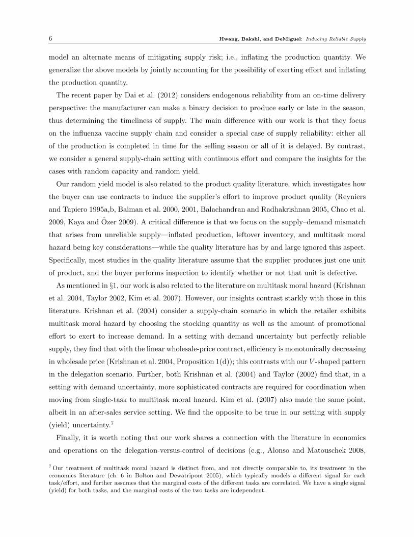
Figure 3 Efficiency of Wholesale-Price Contracts under Random Capacity
This figure depicts the supply chain efficiency (vertical axis) for random capacity when the wholesale price (horizontalaxis) ranges between the unit production cost c and the price p for the case with parameters D = 100,K = 120, p=10, c= 2, θ= 100, and m= 2.
2 4 6 8 1075
80
85
90
95
100
Wholesale Price
Eff
icie
ncy
(%
)
[0,K/(e+ 1)]. The expected cost is c(q, e) = cy(q, e) + θem, where c, θ > 0 and m> 1.
Figure 3 shows the supply-chain efficiency (vertical axis) when the wholesale price (horizontal
axis) ranges between the unit production cost c and the price p for the case with parameters
D = 100,K = 120, p= 10, c= 2, θ = 100, and m= 2. We observe that the efficiency monotonically
increases with the wholesale price w in the entire range [c, p]. Also, the efficiency can be relatively
low (77%) when the buyer has complete bargaining power (w = c). We repeated this experiment
with 2,401 different parameter combinations. Specifically, because the qualitative results do not
depend on the scale of the problem, we fixed the demand to D= 100 and the retail price to p= 10,
and then varied other parameters. We chose seven values for each of K,c, θ, and m in the following
ranges including the boundary values: K = [110,300], c = [0.1,7], θ = [1,200], and m = [1.01,5].
We analyzed the inefficiency with all 74 = 2,401 combinations. We found that the buyer ordered
exactly D in 95.7% of cases8, and the efficiency was monotonically increasing in the entire range of
wholesale prices [c, p] in 99.29% of cases. The remaining 0.71% cases correspond to an unrealistically
low unit production cost of c= 0.1, which is 1% of the price. Moreover, we find that even for these
cases with c= 0.1, the efficiency is increasing in the wholesale price except for very low wholesale
prices, i.e., w close to c.9
8 We find that in 4.3% of cases the buyer finds it optimal to inflate her order quantity despite the fact that this doesnot directly increase the chance that she will get D units delivered. The reason for this is that order inflation helpsindirectly by giving the supplier incentives to exert more effort to improve reliability.
9 Our observations are robust to the use of the triangular distribution. Specifically, efficiency is monotonically increas-ing in the wholesale price in 99.21% of cases. Moreover, the remaining 0.79% of cases correspond to very low unitproduction costs, and the efficiency trend is preserved except for very low wholesale prices.

Hwang, Bakshi, and DeMiguel: Inducing Reliable Supply 13
Thus, we find that the intuition we obtained from Proposition 2 holds in general and that
efficiency is monotonically increasing in the supplier’s bargaining power. Hence, it suffices to use
the wholesale-price contract if the supplier is powerful, but we have yet to determine what the best
option is otherwise.
We find that unit-penalty contracts coordinate the supply chain, while allowing flexibility in
profit-allocation between the buyer and the supplier. Under such contracts, the buyer imposes
a penalty z for each unit of shortage, while paying w for each unit delivered. The next result
formalizes our findings.
Proposition 3. Let Assumptions 1 and 2 hold. Then, there exists χ > 0 such that the following
unit-penalty contracts coordinate the supply chain: w∗ = p−χ and z∗ = χ, where χ∈ [0, χ); and the
buyer’s expected profit is πb = χD.
By setting the unit-penalty z equal to her unit margin p−w, the buyer earns a fixed profit of z
for each unit of demand from either sale or penalty. The buyer does not inflate the order if the unit
penalty is not too large and is therefore able to induce the same economic trade-offs for the supplier
as the centralized decision maker, i.e., the supplier faces a per-unit underage cost that comprises
his own margin, w − c, plus the unit-penalty, p−w, which together add up to the supply chain
margin, p− c. As a result, the supplier exerts the first-best effort. Flexibility in profit allocation
is achieved by varying w. Thus, with random capacity, bargaining power plays a key role: the
wholesale-price contract suffices when the supplier is powerful, and a unit-penalty contract may
be used to good effect otherwise. Would these insights continue to hold if the nature of supply
risk is altered to random yield instead, or does bargaining power interact with supply risk in a
qualitatively different manner? We address this question next.
5. Random Yield
With random yield, we model disruptions in which the random loss is stochastically proportional
to the production quantity, i.e., a larger production quantity increases the likelihood of obtaining
a larger amount of usable output (Federgruen and Yang 2008, 2009a,b, Tang and Kouvelis 2011).
It applies, for example, when manufacturers of semiconductor or biotech products face uncertain
yield in their manufacturing processes. The key distinguishing feature from random capacity is
that, in addition to effort, now inflating the production quantity (above demand) can be used as
an additional lever to mitigate supply risk.
Following the literature, we study two different cases that depend on the supplier’s decision
regarding production quantity. In §5.1 we examine the “control” scenario, in which the buyer
dictates the supplier’s production quantity decision, and in §5.2 we investigate the “delegation” sce-
nario, in which the supplier independently decides his production quantity, given the buyer’s order.

14 Hwang, Bakshi, and DeMiguel: Inducing Reliable Supply
For each case, we show how the basic model of §3 can be applied, and discuss the corresponding
simplicity–efficiency trade-off in contract choice.
5.1. Control Scenario
Federgruen and Yang (2009a) study a setting in which the buyer dictates the supplier’s production
quantity. They explain that this formulation is appropriate for contexts in which the supplier
cannot undertake full inspection of all produced units at his site.10 In such cases, even though the
buyer will inflate her order quantity to buffer against yield losses, the supplier will produce and
deliver exactly this quantity for practical reasons: in accordance with the order quantity, the buyer
would have planned her supporting infrastructure, e.g., warehousing space, testing equipment, and
staff, and would therefore not accept anything in excess of her order quantity.
While the above is a context-based explanation for the control scenario, this model setup serves
another crucial purpose in our paper that broadens the scope of its applicability: it allows us to
pose the question, if the control setup is not a compulsion but an option, would the buyer then
prefer to control or delegate the production decision?
5.1.1. Model and Centralized Supply Chain. The supplier delivers a random quantity
q = (1− ξ)q, where q is the order quantity and ξ is the random proportional loss. To focus on the
effect of the random proportional loss, we assume in our model with random yield that the supplier
has no capacity constraints. We further assume that the random loss is ξ = fy(ψ,e), where ψ is
a random variable that captures the underlying supply risk and fy is a function that models the
dependence of the random loss on the supplier’s effort e. We denote the density and CDF of the
random proportional loss as h(ξ | e) and H(ξ | e), respectively, and the expected random loss as
E[ξ] = µey. The expected delivered quantity and sales are y(q, e) =Eξ[q] and S(q, e) =Eξ[min{q,D}],
respectively.
We assume the supplier incurs the production cost for all q units. This is reasonable as yield
and quality problems generally arise after all raw materials have been put into the production line.
Hence, the cost is c(q, e) = cq+ v(e). Additionally, we make the following technical assumption.
Assumption 3. The following conditions hold:
(i) The random loss ξ has support [0, ay(e)], with ay(0) = 1 and ay(e) ≤ 1. Moreover, ay(e) is
twice continuously differentiable and a′y(e)≤ 0 for e≥ 0.
(ii) The CDF, H(ξ | e), is thrice continuously differentiable with finite derivatives in ξ ∈ [0, ay(e)]
and e≥ 0, and ∂H(ξ | e)/∂e > 0, ∂2H(ξ | e)/∂e2 ≤ 0 for ξ ∈ (0, ay(e)) and e≥ 0.
10 Full inspection at the supplier’s site is often impossible or impractical (e.g., Baiman et al. 2000, Balachandran andRadhakrishnan 2005), particularly when failures are mainly observed externally by the consumer (e.g., Kulp et al.2007), or when the testing technology is proprietary and the buyer deliberately limits the supplier’s ability to detectfailures due to intellectual property concerns (p23, Doucakis 2007).
Hwang, Bakshi, and DeMiguel: Inducing Reliable Supply 15
(iii) The cost of effort is thrice continuously differentiable and satisfies v(0) = v′(0) = 0 and
v′(e), v′′(e)> 0 for e > 0.
A few comments on Assumption 3 are in order. Part (i) implies that the entire production
quantity is subject to random loss in the absence of supplier effort (ay(0) = 1), but the supplier’s
effort may (or may not) reduce the range of the loss (ay(e)≤ 1). Part (ii) implies that the effort
e mitigates the random loss ξ in the sense of first-order stochastic dominance with decreasing
returns to scale. Part (iii) implies that the cost of the supplier’s effort is convex and increasing,
and assuming v′i(0) = 0 guarantees interior solutions.
An interesting property of the random yield model with control is that, unlike for the random
capacity model, the expected sales increase in the order quantity even if the order quantity is larger
than the demand (q > D). This is because the random loss is stochastically proportional to the
order quantity q and ordering more can therefore increase the probability that the supplier will
deliver D units, increasing the expected sales. The technical properties of expected sales, S(q, e),
and expected delivered quantity, y(q, e), are summarized in Lemma 3 in Appendix A.2. We can
now characterize the optimal decisions in the centralized supply chain.
Proposition 4. Let Assumptions 1 and 3 hold. Then, in the centralized supply chain with
random yield, there exist optimal order quantity qo and effort level eo that satisfy the first-order
necessary conditions: p ∂S(qo, eo)/∂q= c and p ∂S(qo, eo)/∂e= v′(eo). Moreover, the optimal order
quantity satisfies D< qo <D/(1− ay(eo)).
The optimal decisions differ qualitatively from those for random capacity in Proposition 1; it is
now optimal for the buyer to order more than the demand (qo >D). In other words, the decision
maker increases the expected profit by not only exerting effort but also ordering more. It is optimal
to order more than D because it increases expected sales, S(q, e), and the marginal benefit of such
an increase at q=D, which is p∂S(D,e)/∂q, is larger than the marginal cost c, a result that follows
from Assumption 1(i). Based on this understanding, one might expect that in a decentralized
setting the need to coordinate the buyer’s order inflation, in addition to the supplier’s effort, will
give rise to different and more subtle dynamics relative to random capacity. We investigate these
issues next.
5.1.2. Simplicity–Efficiency Trade-Off. Once again we start with the treatment of the
linear wholesale-price contract, but this time we find that the efficiency of a wholesale-price contract
decreases in the supplier’s bargaining power. This is in sharp contrast to the result in the random
capacity model, in which the efficiency of the wholesale-price contract increases in the supplier’s
bargaining power. Therefore, the wholesale-price contract is more likely to be the preferred mode

16 Hwang, Bakshi, and DeMiguel: Inducing Reliable Supply
of contracting when the buyer is powerful. Again, to reach this conclusion, we employ a mix
of analytical and numerical investigations. First, we analytically show that the efficiency of the
wholesale-price contract monotonically decreases with the wholesale price w when the wholesale
price w is above a certain threshold.
Proposition 5. Let Assumptions 1 and 3 hold. Then, for random yield with control, there exists
wc < p such that the efficiency of a wholesale-price contract monotonically decreases in w ∈ [wc, p].
This result contrasts directly with that for random capacity in Proposition 2, in which the
efficiency increases in w above a certain threshold. Intuitively, a more powerful buyer (low w) has
a greater incentive to inflate her order, which helps increase efficiency, but a less powerful supplier
has a smaller incentive (low margin) to invest in reliability improvement, which hurts efficiency.
However, the latter effect is mitigated by two factors that together result in the observed efficiency
trend. First, when w is low and the buyer inflates the order, the supplier does not bear the cost of
overage (leftover inventory) and hence exerts “more-than-expected” effort, which results in high
efficiency. Second, both order inflation and effort have diminishing marginal impact on the expected
sales. Moreover, even without inflation, the buyer orders at least the demand quantity, regardless of
the wholesale price; this already induces a certain amount of effort. Hence, when w is high, on the
one hand the supplier exerts more effort but its marginal impact in terms of increasing expected
sales is limited; on the other hand, the buyer barely inflates the order (due to the low margin) and
this has a greater marginal impact in terms of decreasing the expected sales. We therefore observe
low efficiency overall. As a result of these two asymmetric effects, we can expect high efficiency
when w is low and low efficiency when w is high.
The above intuition suggests that the monotonicity trend in efficiency ought to hold through the
entire range w ∈ [c, p]. In order to verify this conjecture, we conduct a comprehensive numerical
investigation. As with random capacity, we rely on the uniform and triangular distribution
for modeling the loss distribution, H(ξ|e), and mainly emphasize the results with the uniform
distribution. The corresponding numerical setup is described below.
NUMERICAL SETUP 2: (Random Yield) Let ξ = fy(ψ,e) =ψ/(e+ 1). ψ is uniformly distributed
in [0,1]. Then, h(ξ | e) = e + 1 and H(ξ | e) = (e + 1)ξ with support [0,1/(e + 1)]. The cost is
c(q, e) = cq+ θem, where c, θ > 0 and m> 1.
Even this seemingly simple model is analytically intractable; we are not able to obtain explicit
expressions for the optimal decisions or supply-chain efficiency. However, Figure 4 displays the
outcome of numerical analysis for the same set of parameters as for Figure 3. We observe a very

Hwang, Bakshi, and DeMiguel: Inducing Reliable Supply 17
Figure 4 Efficiency of Wholesale-Price Contracts under Random Yield with Control
This figure depicts the efficiency (vertical axis) under random yield with control when the wholesale price (horizontalaxis) ranges between the unit production cost c and the price p for the case with parameters D = 100, p = 10, c =2, θ= 100, and m= 2. Note that, for random yield, when the wholesale price w is close to the unit production cost c,there is no feasible solution because the supplier’s participation constraint cannot be satisfied.
2 4 6 8 1080
85
90
95
100
Wholesale Price
Eff
icie
ncy
(%
)
robust decreasing trend in efficiency. Specifically, the efficiency is fairly high (∼ 98%) when the
buyer is powerful but is relatively low (∼ 80%) when the supplier is powerful. We then repeated
our experiment with different parameter combinations; we chose seven values each for c, θ, and m
in the following ranges: c= [0.1,7], θ = [1,200],m= [1.01,5]. We therefore performed our analysis
with 73=343 different combinations of parameters. We found that the efficiency was monotoni-
cally decreasing in the entire range of wholesale prices in 93.6% of cases. The remaining 6.4% of
cases exhibited a slight increase for small w only, but the general decreasing trend was preserved
elsewhere.11
Thus, the nature of the supply risk interacts with bargaining power in subtle and non-obvious
ways to determine the ability of the wholesale-price contract to induce reliable supply. Specifically,
we find that, for random yield with control, efficiency is monotonically decreasing in the supplier’s
bargaining power, while the exact opposite is true for random capacity. This is arguably a surprising
result: intuition would suggest that the problem of incentive alignment is mitigated (i.e., supply-
chain efficiency is higher) as the agent undertaking unverifiable action is awarded a higher margin
and thereby made better off; the efficiency trend for random yield with control is the opposite.
We have yet to address the question of which contract to use when the efficiency engendered by
the wholesale-price contract is low. With random capacity, the unit-penalty contract coordinates
the supply chain: How does it fare under random yield with control? Our next result answers this
question.
11 We explored the triangular distribution with the same combinations of parameters and found complete monotonicityin efficiency in 100% of cases.
18 Hwang, Bakshi, and DeMiguel: Inducing Reliable Supply
Lemma 1. Let Assumptions 1 and 3 hold. A unit-penalty contract cannot coordinate the supply
chain except when the buyer secures the entire supply-chain profit.
For the unit-penalty contract to coordinate, the buyer must keep the entire supply chain profit;
thus, the unit-penalty contract fails to coordinate in situations in which the buyer does not possess
all the bargaining power.12 The reason the unit-penalty contract fails to coordinate in most situa-
tions is that even though it is optimal for the buyer to inflate her order quantity above demand, the
supplier does not partake in the overage risk, i.e., the supplier does not bear any direct cost from
leftover inventory. As a result, the unit-penalty contract fails to exactly replicate for the supplier
the trade-offs faced by a centralized decision maker (except when the buyer keeps all the profits).
One obvious way to share the overage cost is through a buy-back agreement. Indeed, we find that
a unit-penalty with buy-back contract coordinates the supply chain while allowing for arbitrary
profit allocation between the buyer and supplier. Under a unit-penalty with buy-back contract, the
buyer pays a wholesale price w for each unit delivered, and the supplier pays a unit penalty z for
each unit of shortage and buys back leftover inventory at a unit buy-back price b.
Proposition 6. Let Assumptions 1 and 3 hold. There exists a continuum of unit-penalty with
buy-back contracts that satisfy the Karush–Kuhn–Tucker (KKT) conditions at (qo, eo) in optimiza-
tion problem (2), allowing arbitrary profit allocation.
Although Proposition 6 checks only the KKT conditions, we find that a unit-penalty with buy-
back contract does coordinate the supply chain with all parameters considered under Numerical
Setup 2.
In this section, we have established that the insights that emerge for random yield with control
are substantially different to those for random capacity, thereby underlining the pivotal role of the
interaction between supply risk and bargaining power in determining the performance of incentive
contracts aimed at inducing reliable supply. We next address the final piece in this mix: delegation-
versus-control choices. In particular, we investigate what happens when the buyer delegates the
production quantity decision to the supplier under random yield.
5.2. Delegation Scenario
There are a number of contexts that support the delegation of the production quantity decision to
the supplier; e.g., Chick et al. (2008) and Tang et al. (2014). This leads to the possibility of both the
buyer and the supplier inflating the order quantity and the production quantity, respectively. This
12 We have numerically analyzed the efficiency of unit-penalty contracts; the insight is analogous to that from the useof wholesale-price contracts: the supply-chain efficiency induced by a unit-penalty contract decreases in the supplier’sbargaining power, i.e., as the wholesale-price, w, increases or the penalty, z, decreases. Since the insight, and therationale behind it, is very similar to that obtained with wholesale-price contracts, we do not go into more detail.
Hwang, Bakshi, and DeMiguel: Inducing Reliable Supply 19
aspect introduces an additional source of inefficiency into the supply chain: the supplier potentially
inflates the production quantity, even if the buyer has already padded her order quantity to buffer
against yield losses. These buffers may accumulate and exacerbate inefficiency. Furthermore, the
paradigm of multitask moral hazard reinforces the expectation that efficiency will be lower in the
delegation scenario, since it requires the coordination of two unverifiable actions of the agent: effort
and production quantity. We now examine whether this is indeed the case.
5.2.1. Model and Centralized Supply Chain. The model is similar to that of the control
scenario in §5.1 except that the supplier determines his own production quantity x. Therefore, we
present only those parts of the model that are different from the control scenario. The supplier
delivers a random quantity q= min{q, (1− ξ)x}, where q is the order quantity, x is the production
quantity, and ξ is the random proportional loss as defined in §5.1. The expected delivered quantity
is represented as y(q,x, e) = Eξ[q] and the expected sales, S(q,x, e) = Eξ[min{q,D}]. The cost is
c(x, e) = cx+ v(e). For tractability, we also make the following assumption.
Assumption 4. The expected delivered quantity y(q,x, e) is jointly concave in q and e, and also
in x and e in the feasible region in problem (2).
While it is difficult to establish the above property in general, we have verified analytically that it
is satisfied by the uniform distribution, as used in Numerical Setup 2.
Unlike the control scenario, if the order quantity is larger than the demand (q >D), the expected
sales become constant, as in the random capacity model. This is because as long as q ≥D, the
probability of receiving D units depends only on the production quantity x and the effort e.
Therefore, ordering more than D does not directly increase the expected sales and S(q,x, e) has a
kink at q=D. Note, however, that higher q does give the supplier an incentive to choose higher x
and e, and can thereby indirectly increase expected sales. The properties of S(q,x, e) and y(q,x, e)
are summarized in Lemma 4 in Appendix A.3.
In the centralized supply chain, the order quantity is redundant, and the decision maker chooses
only the production quantity x and the effort e. Therefore, the optimal decisions in the centralized
supply chain are the same as for the control case discussed in §5.1 except that we replace the order
quantity q with the production quantity x in Proposition 4 and refer to the optimal production
quantity as xo. We examine the decentralized setup next.
5.2.2. Simplicity–Efficiency Trade-Off. We discover that the efficiency associated with
the wholesale-price contract exhibits a V -shaped pattern as we increase the supplier’s bargaining
power; this contrasts with both the random capacity model and the random yield with control
scenario. Therefore, we argue that with the delegation of the production quantity decision, if either
20 Hwang, Bakshi, and DeMiguel: Inducing Reliable Supply
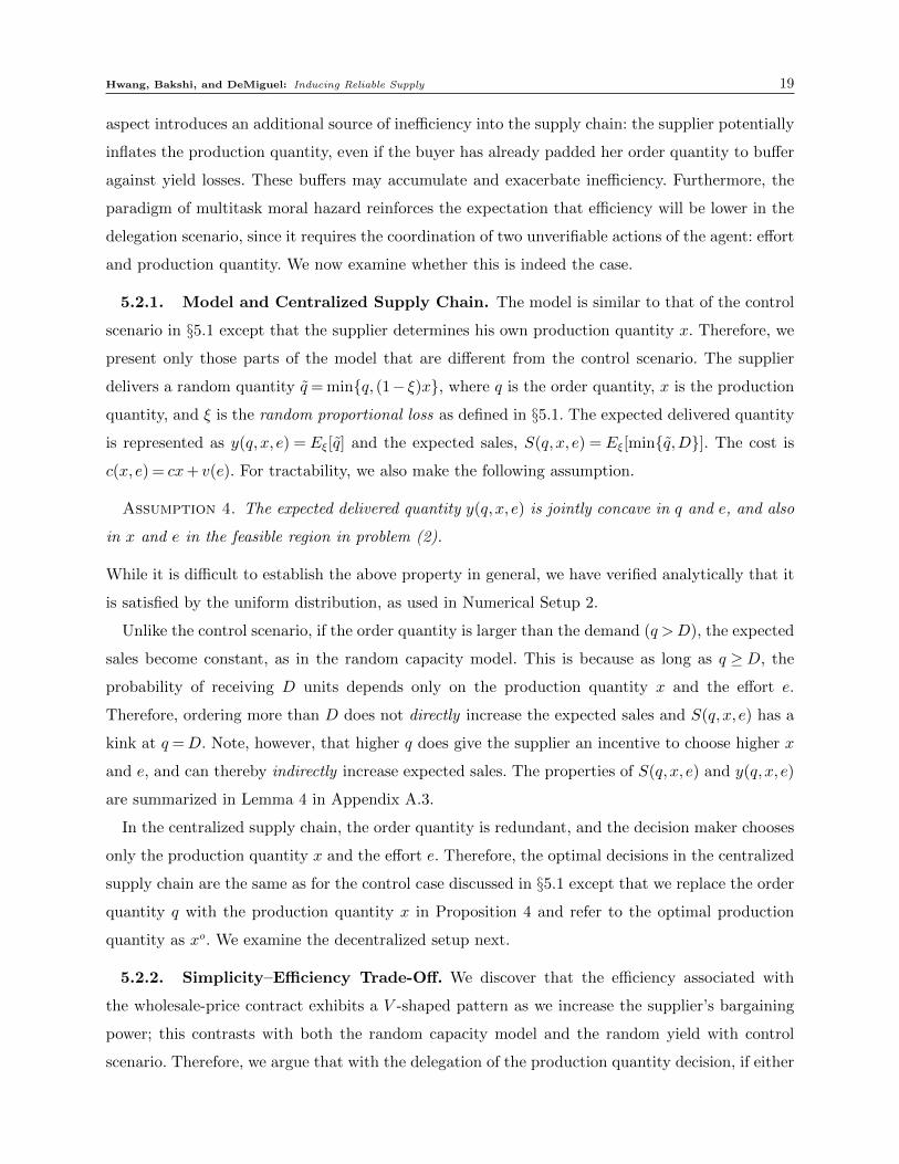
Figure 5 Efficiency of Wholesale-Price Contracts under Random Yield with Delegation
This figure depicts the efficiency (vertical axis) under random yield with delegation when the wholesale price (hor-izontal axis) ranges between the unit production cost c and the price p for the case with parameters D = 100, p =10, c= 2, θ= 100, and m= 2.
2 4 6 8 1095
96
97
98
99
100
Wholesale Price
Eff
icie
ncy
(%
)
party possesses the bulk of the bargaining power, then the wholesale-price contract is likely to be
the preferred mode of contracting, even if more complex contracts that offer theoretically better
performance exist.
Once again, we employ a mix of analytical and numerical investigations to substantiate our
claim. First, we analytically show that if w is sufficiently large, the efficiency of a wholesale-price
contract monotonically increases. This corresponds to the right-hand side of the V -shape.
Proposition 7. Let Assumptions 1, 3, and 4 hold. Then, there exists wd < p such that the
efficiency associated with a wholesale-price contract monotonically increases in w ∈ [wd, p].
The intuition for the above result is as follows. The wholesale price, wd, is the threshold below
which the buyer inflates the order and above which the buyer orders only D units. Such a threshold
exists because the buyer’s order inflation only indirectly increases the expected sales: by allowing
the supplier to sell more units, order inflation induces a larger production quantity and greater
effort from the supplier. For w ≥ wd, the buyer’s margin is too low to incentivize her to inflate;
she orders exactly the demand quantity. Thus, above the threshold wd, the supplier unilaterally
determines effort and inflation; hence, efficiency increases monotonically in the wholesale price
(due to the higher supplier margin). At w= p, the supply chain is coordinated. Finally, below the
threshold, wd, we reason that the dynamics are similar to those in the control scenario and expect
a similar trend: efficiency is monotonically decreasing in w, thereby giving rise to the V -shaped
trend in efficiency.
Second, we numerically verify this intuition by examining the efficiency pattern of a wholesale-
price contract in the entire bargaining power spectrum. We do so by adapting Numerical Setup
2 to the delegation scenario. Figure 5 shows that efficiency follows a clear V -shaped pattern as a
Hwang, Bakshi, and DeMiguel: Inducing Reliable Supply 21
function of the wholesale price. The lowest efficiency is 95.9% at wd. When w is low, the efficiency
rises to 98.3%, and when w is high, the efficiency goes up to 100%. We analyzed 343 different cases
with the same parameter combinations as in §5.1 and observe an unambiguous V -shape in 77.45%
of cases. In 14.71% of cases, we again observe a prominent V -shape, but with a slight increase
in efficiency (typically less than 0.1%) when w is very low (on the left extreme of the bargaining
power spectrum), followed by the expected V -shaped pattern. In the remaining 7.84% of cases, the
efficiency is just increasing, but these are exceptional cases when the unit production cost c is so
high (more than half the retail price p) that feasible solutions exist only when the wholesale price
w is at least as large as 90% of the retail price; effectively, w>wd in the feasible region.13
Our results above suggest that when thinking about using incentives to induce reliable supply
in a decentralized supply chain, one must consider whether the buyer controls or delegates the
production quantity decision, in addition to bargaining power and the nature of supply risk. Inter-
estingly, for the delegation scenario, we find that as we increase the margin (and therefore payoff)
of the supplier (the agent undertaking unverifiable action), the trend in efficiency is neither mono-
tonically increasing (as with random capacity) nor monotonically decreasing (as with random yield
with control), but is instead V -shaped.
The issue of delegation versus control certainly warrants further investigation. In particular,
how do the individual parties fare in the delegation scenario relative to the control scenario?
How does efficiency compare in the two scenarios? The reasoning given at the beginning of this
section suggests that multitask moral hazard in the delegation scenario would be detrimental for
supply-chain efficiency and, therefore, if given a choice, the buyer would perhaps opt to control
the production decision. We now verify whether this line of thinking bears out.
Comparison between control and delegation outcomes: In order to facilitate the discussion
we introduce some new notation. We denote the supplier’s expected profit in the control and
delegation scenarios by πcs and πds , respectively. The corresponding notation for the buyer is πcb and
πdb , and the centralized profit is represented as Π(xo, eo). Also, we define ∆πs(%)≡ πds−πcs
Π(xo,eo)× 100,
∆πb(%)≡ πdb−πcb
Π(xo,eo)× 100, and the change in efficiency is ∆Eff.(%)≡∆πb + ∆πs.
In Figure 6, Panels (a) and (b) show ∆πb and ∆πs in the context of Numerical Setup 2. We
vary the unit production cost c from 0.5 to 3, while fixing the other parameters at D = 100, p=
10, θ= 100, and m= 2. Perhaps surprisingly, we observe that the buyer is “always” better off with
delegation, and the increase in her expected profit can be as large as 10% of the centralized profit.
13 With the triangular distribution, we observe an unambiguous V -shape in 84.66% of cases. Also, in 7.42% of cases,we find a prominent V -shape but with a slight increase in efficiency at the left extreme of the V . In 7.92% of cases,the efficiency was just increasing; but again, these cases have a very high unit production cost c and feasible solutionstherefore exist only when the wholesale price w is at least 90% of the retail price p.
22 Hwang, Bakshi, and DeMiguel: Inducing Reliable Supply
Figure 6 Comparisons of Two Scenarios under Random Yield with Different Unit Production Costs
Panels (a), (b), and (c) depict ∆πb, ∆πs, and ∆Eff., respectively. We vary the unit production cost c from 0.5 to 3,while fixing the other parameters as follows: D= 100, p= 10, θ= 100, and m= 2.
0 2 4 6 8 100
2
4
6
8
10
12
Wholesale Price
∆ B
uye
r P
rofi
t (%
)
c=0.5c=1c=2c=3
(a) Differences in Buyer Profit, ∆πb
0 2 4 6 8 10−10
−5
0
5
10
15
20
25
30
Wholesale Price
∆ S
up
plie
r P
rofi
t (%
)
c=0.5c=1c=2c=3
(b) Differences in Supplier Profit, ∆πs
0 2 4 6 8 10−5
0
5
10
15
20
25
30
Wholesale Price
∆ E
ffic
ien
cy (
%)
c=0.5c=1c=2c=3
(c) Differences in Efficiency, ∆Eff.
The supplier, however, is worse off with delegation when the buyer is powerful, i.e., when w is low.
The supplier is better off only when she has a certain amount of bargaining power, i.e., when w
is above a certain threshold, and the increase in his expected profit can be as large as 28%. Panel
(c) in Figure 6 shows the resulting differences in efficiency: when w is low, the efficiency remains
constant (it is slightly lower for the delegation scenario), but as w increases, the efficiency increases
dramatically up to 28% higher in the delegation scenario.
In Figure 7, Panels (a) and (b) show how ∆πb and ∆πs change for costs of effort θ ranging
between 10 and 150, while fixing the other parameters at D= 100, p= 10, c= 2, and m= 2. Panel
(c) in Figure 7 shows the resulting differences in efficiency. We observe a similar result as before.
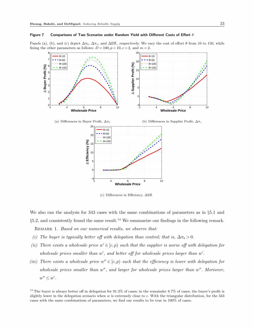
Hwang, Bakshi, and DeMiguel: Inducing Reliable Supply 23
Figure 7 Comparisons of Two Scenarios under Random Yield with Different Costs of Effort θ
Panels (a), (b), and (c) depict ∆πb, ∆πs, and ∆Eff., respectively. We vary the cost of effort θ from 10 to 150, whilefixing the other parameters as follows: D= 100, p= 10, c= 2, and m= 2.
2 4 6 8 100
1
2
3
4
5
6
7
8
Wholesale Price
∆ B
uye
r P
rofi
t (%
)
θ=10θ=50θ=100θ=150
(a) Differences in Buyer Profit, ∆πb
2 4 6 8 10−5
0
5
10
15
20
25
Wholesale Price
∆ S
up
plie
r P
rofi
t (%
)
θ=10θ=50θ=100θ=150
(b) Differences in Supplier Profit, ∆πs
2 4 6 8 10−5
0
5
10
15
20
25
Wholesale Price
∆ E
ffic
ien
cy (
%)
θ=10θ=50θ=100θ=150
(c) Differences in Efficiency, ∆Eff.
We also ran the analysis for 343 cases with the same combinations of parameters as in §5.1 and
§5.2, and consistently found the same result.14 We summarize our findings in the following remark.
Remark 1. Based on our numerical results, we observe that:
(i) The buyer is typically better off with delegation than control; that is, ∆πb > 0.
(ii) There exists a wholesale price w′ ∈ [c, p) such that the supplier is worse off with delegation for
wholesale prices smaller than w′, and better off for wholesale prices larger than w′.
(iii) There exists a wholesale price w′′ ∈ [c, p) such that the efficiency is lower with delegation for
wholesale prices smaller than w′′, and larger for wholesale prices larger than w′′. Moreover,
w′′ ≤w′.
14 The buyer is always better off in delegation for 91.3% of cases; in the remainder 8.7% of cases, the buyer’s profit isslightly lower in the delegation scenario when w is extremely close to c. With the triangular distribution, for the 343cases with the same combinations of parameters, we find our results to be true in 100% of cases.

24 Hwang, Bakshi, and DeMiguel: Inducing Reliable Supply
The reason for our somewhat counter-intuitive results lies in how the inventory risk is allocated
in the supply chain (Cachon 2004). Specifically, the explanation for part (i) is that in the control
scenario, the supplier is precluded from sharing any overage cost because he cannot inflate the
production quantity, while in the delegation scenario, the supplier is free to inflate as required. This
additional flexibility for the supplier is deceptive because the buyer anticipates the supplier’s best
response and adjusts her order quantity to induce optimal (for her) sharing of the overage risk:
the supplier now bears the overage cost for units produced in excess of the buyer’s order quantity.
Thus, by virtue of reallocating the inventory risk in the supply chain, the buyer finds that she is
better off delegating the production decision to the supplier. The above also forms the basis for the
observation in part (ii). Although one might expect that the supplier would always be better off in
the delegation scenario owing to the additional flexibility in decision making (the supplier chooses
effort as well as production quantity), an offsetting influence is introduced as he now shares the
overage risk. The latter effect dominates when the buyer is powerful (low wholesale price). Finally,
combining the insights from parts (i) and (ii) provides the basis for understanding the result in
part (iii), because the efficiency is determined by the sum of both firms’ profits. It is worth noting
that the loss in efficiency, when it occurs, is minimal (generally less than 1.5%), while the gain in
efficiency can be great (between 10% and 30%).
Because the sharing of the overage risk is the main driver of the results in Remark 1, we expect
the effects to be more pronounced if the unit production cost is relatively cheaper than the cost
of effort and production inflation therefore plays a more important role than exerting effort in
mitigating the supply risk. Figures 6 and 7 confirm this insight. In these figures, the effects are
more pronounced as the unit production cost c decreases or the cost of effort θ increases.
Thus, it seems that, in a setting with unreliable supply (random yield), multitask moral hazard
(delegation scenario) can actually mitigate the incentive alignment challenge for the buyer and
improve supply-chain efficiency. To consolidate this insight, there is still one remaining loose end:
how do the coordinating contracts contrast between the delegation and control scenarios? We
address this next.
Proposition 8. Let Assumptions 1, 3, and 4 hold. There exists χ > 0 such that the following
unit-penalty contracts coordinate the supply chain: w∗ = p− χ, z∗ = χ, where 0 ≤ χ ≤ χ; and the
buyer’s expected profit is πdb = χD.
Interestingly, we find that a unit-penalty contract coordinates the supply chain with flexible profit
allocation, even though there exists an additional dimension of moral hazard (production quantity)
in comparison to the control scenario, which requires the more complex unit-penalty with buy-
back contract for coordination. This result is consistent with our findings for the wholesale-price

Hwang, Bakshi, and DeMiguel: Inducing Reliable Supply 25
contract, but runs counter to the intuition suggested by the existing literature on multitask moral
hazard. Krishnan et al. (2004) and Taylor (2002) have studied multitask moral hazard in a context
that is analogous to ours: while our setting pertains to supply uncertainty with supply-enhancing
effort, they study demand uncertainty with demand-enhancing effort. Both papers find that the
coordinating contract increases in complexity as we move from single-dimensional to multitask
moral hazard; the opposite is true for our findings.15
A lesson from our findings is that the insights from the seemingly analogous context of demand
uncertainty do not carry over to the context of supply uncertainty. According to Krishnan et al.
(2004), when agents perform multiple tasks: “moral hazard problems may interact, necessitating
complex supply chain contracts that still fall short of the first best, in part because individual
contract terms can work at cross purposes, helping one incentive conflict but exacerbating another.”
By contrast, the unit-penalty in Proposition 8 coordinates both actions: production quantity and
effort. The intuition is that if the penalty fee is set equal to the margin (and is not too large), then
the buyer does not inflate the order, because for each unit of demand she can make her margin
through either a sale or the penalty imposed on the supplier. Then, the supplier faces exactly
the same trade-offs as the centralized decision maker and thus chooses the first-best effort and
production quantity.
6. Managerial Implications and Conclusions
We have investigated the use of incentives in inducing reliability-improving effort from the supplier
in a decentralized supply chain. We characterize how performance in the supply chain depends on
the interplay between the nature of supply risk, the balance of bargaining power, and whether the
buyer controls or delegates the production quantity decision. Our objective requires us to revisit
the classic moral hazard problem in the context of unreliable supply. We find that a number of
“common intuitions” acquired from analogous contexts do not carry over to our setting, and this
has significant managerial implications. We summarize our two major findings below.
Moral Hazard and the use of Appropriate Contracts: Heuristic reasoning suggests that as
an agent undertaking unverifiable action makes a greater profit, he will have a greater incentive to
invest in unverifiable actions; this would mitigate the incentive alignment challenge and alleviate
system inefficiency. We find this to be perfectly true for our setting with random capacity. However,
15 Also, Krishnan et al. (2004) find that with the linear wholesale-price contract, efficiency is monotonically decreasingin wholesale price (Proposition 1(d)); this contrasts with our V -shaped pattern in the delegation scenario. Anotherpaper that has studied multitask moral hazard, albeit in an after-sales services context, is Kim et al. (2007); unlikeus, they too find that the coordinating contract increases in complexity when moving from single task to multitaskmoral hazard.
26 Hwang, Bakshi, and DeMiguel: Inducing Reliable Supply
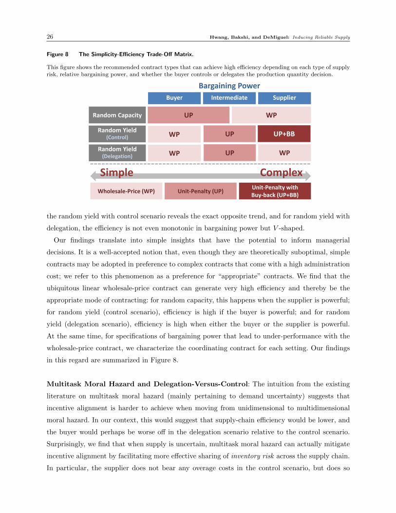
Figure 8 The Simplicity-Efficiency Trade-Off Matrix.
This figure shows the recommended contract types that can achieve high efficiency depending on each type of supplyrisk, relative bargaining power, and whether the buyer controls or delegates the production quantity decision.
Random Capacity
Buyer
WP UP
Supplier
Random Yield (Delegation) WP WP UP
Intermediate
Bargaining Power
Complex Simple
Wholesale-Price (WP) Unit-Penalty (UP) Unit-Penalty with Buy-back (UP+BB)
Random Yield (Control) WP UP UP+BB
the random yield with control scenario reveals the exact opposite trend, and for random yield with
delegation, the efficiency is not even monotonic in bargaining power but V -shaped.
Our findings translate into simple insights that have the potential to inform managerial
decisions. It is a well-accepted notion that, even though they are theoretically suboptimal, simple
contracts may be adopted in preference to complex contracts that come with a high administration
cost; we refer to this phenomenon as a preference for “appropriate” contracts. We find that the
ubiquitous linear wholesale-price contract can generate very high efficiency and thereby be the
appropriate mode of contracting: for random capacity, this happens when the supplier is powerful;
for random yield (control scenario), efficiency is high if the buyer is powerful; and for random
yield (delegation scenario), efficiency is high when either the buyer or the supplier is powerful.
At the same time, for specifications of bargaining power that lead to under-performance with the
wholesale-price contract, we characterize the coordinating contract for each setting. Our findings
in this regard are summarized in Figure 8.
Multitask Moral Hazard and Delegation-Versus-Control: The intuition from the existing
literature on multitask moral hazard (mainly pertaining to demand uncertainty) suggests that
incentive alignment is harder to achieve when moving from unidimensional to multidimensional
moral hazard. In our context, this would suggest that supply-chain efficiency would be lower, and
the buyer would perhaps be worse off in the delegation scenario relative to the control scenario.
Surprisingly, we find that when supply is uncertain, multitask moral hazard can actually mitigate
incentive alignment by facilitating more effective sharing of inventory risk across the supply chain.
In particular, the supplier does not bear any overage costs in the control scenario, but does so
Hwang, Bakshi, and DeMiguel: Inducing Reliable Supply 27
in the delegation scenario. This pivotal observation helps explain why supply-chain efficiency is
invariably higher and the buyer is better off in the delegation scenario compared to the control
scenario. Once again, this insight has important implications for the design of the procurement
process.
In principle, when confronted with yield uncertainty, a powerful buyer may be tempted to impose
her choice of the production decision on the supplier, thinking (perhaps misguidedly) that it would
limit the supplier’s ability to shirk. For example, a powerful buyer of consumer electronics products
such as Hewlett-Packard (HP) is in a position to do so since it retains control over the procurement
process of input materials in-house and only outsources production to the supplier (Supply Chain
Brain 2006, Amaral et al. 2006). Thus, HP can potentially impose the production quantity decision
on its supplier by ensuring that he can only procure inputs up to a limited amount; this amount
corresponds to a pre-determined production quantity. Alternately, if the buyer has exclusive control
over the testing technology (e.g., Doucakis 2007), then she can simply refuse to test more units
than she has ordered, thereby ensuring control over the production decision. However, our results
suggest that such strategies could be counter-productive, and that delegation of the production
quantity decision to the supplier is perhaps a superior alternative from the buyer’s perspective.
Furthermore, if the supplier is powerful, then as per our results, delegation results in a win-win
outcome relative to control and is therefore likely to be the preferred option again.
In conclusion, in light of the growing importance of international sourcing when supply is unreli-
able, our results improve managerial understanding and may be viewed as the building blocks for a
more general model of supply risk that simultaneously incorporates features from random capacity
as well as random yield. Such a model would have a bearing on international sourcing arrangements;
e.g., for a U.S.-based manufacturer sourcing electronic components from China, where supply could
be disrupted by natural disasters in China or yield issues. From a theory-development perspective,
our results on moral hazard suggest the need for a more general theory that can encompass our
findings along with what is already known about this agency issue and about multitask moral
hazard in particular.
Appendix A: Technical Results
A.1. Random Capacity
The following lemma establishes the relationship between expected sales and expected delivered quantity.
Lemma 2. Let Assumption 2 hold. Then:
(i) S(q, e) = y(q, e) if q≤D, and S(q, e) = y(D,e) if q >D; and
28 Hwang, Bakshi, and DeMiguel: Inducing Reliable Supply
(ii) y(q, e) is increasing and concave in q and e.16 Also, y(q, e) is twice continuously differentiable in q and
e, except when q=K − ac(e), where y(q, e) is once continuously differentiable.
The following proposition shows that the efficiency of a wholesale-price contract is monotonically increasing
in the wholesale price provided that the buyer does not inflate her order. We also provide a sufficient condition
for the buyer’s optimal order quantity to be equal to D.
Proposition 9. Let Assumptions 1 and 2 hold. Then:
(i) Provided the buyer’s optimal order quantity is equal to the demand D, the efficiency of a wholesale-price
contract monotonically increases in w ∈ [c, p].
(ii) A sufficient condition for the buyer’s optimal order quantity to be equal to D is
∂G(ξ | e)/∂eG(ξ | e)
<c
p− c· v′′(e)
v′(e)for ξ ∈ [0,K −D], (3)
when e∈ [0, v−1((p− c)K)].17
The sufficient condition (3) suggests that the buyer is more likely to order D if the unit production cost c is
not too small compared to the price p and the cost of effort has high curvature.
A.2. Random Yield: Control Scenario
The following lemma shows the relationship between the expected sales and delivered quantity.
Lemma 3. Let Assumption 3 hold. Then:
(i) If q≤D, then S(q, e) = y(q, e). If q >D, then S(q, e)< y(q, e); and
(ii) y(q, e) and S(q, e) are increasing and concave in q and e.18 Also, y(q, e) and S(q, e) are thrice continu-
ously differentiable in q and e, except that S(q, e) is once continuously differentiable in q when q =D,
and in q and e when q=D/(1− ay(e)).
A.3. Random Yield: Delegation Scenario
The following lemma shows the relationship between the expected sales and delivered quantity. The difference
from the control scenario is that the expected sales are constant provided that the buyer orders at least D
units. Hence, the expected sales S(q,x, e) have a kink at q=D.
Lemma 4. Let Assumption 3 hold. If the supplier determines his own production quantity, then:
(i) If q≤D, then S(q,x, e) = y(q,x, e). If q >D, then S(q,x, e) = y(D,x, e).
(ii) y(q,x, e) is increasing and concave in x and e. Also, y(q,x, e) is thrice continuously differentiable in
x and e, except that it is once continuously differentiable in x when x = q, and in x and e when
x= q/(1− ay(e)).
16 Monotonicity and convexity/concavity are all used in the weak sense throughout the paper. The detailed derivativesare summarized in Table 1 in Appendix B.
17 Note that v−1(·) is an inverse function of v(·), and v′′(e)/v′(e) measures the curvature of v(e), the cost of effort. Itis analogous to the Arrow–Pratt measure of absolute risk aversion.
18 Note that y(q, e) is linear in q. The detailed derivatives are summarized in Table 2 in Appendix B.
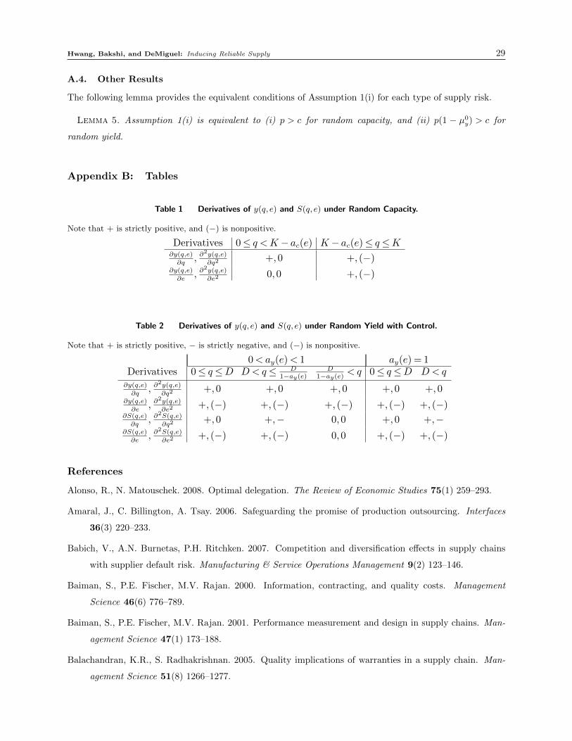
Hwang, Bakshi, and DeMiguel: Inducing Reliable Supply 29
A.4. Other Results
The following lemma provides the equivalent conditions of Assumption 1(i) for each type of supply risk.
Lemma 5. Assumption 1(i) is equivalent to (i) p > c for random capacity, and (ii) p(1 − µ0y) > c for
random yield.
Appendix B: Tables
Table 1 Derivatives of y(q, e) and S(q, e) under Random Capacity.
Note that + is strictly positive, and (−) is nonpositive.
Derivatives 0≤ q <K − ac(e) K − ac(e)≤ q≤K∂y(q,e)
∂q, ∂
2y(q,e)
∂q2+,0 +, (−)
∂y(q,e)
∂e, ∂
2y(q,e)
∂e20,0 +, (−)
Table 2 Derivatives of y(q, e) and S(q, e) under Random Yield with Control.
Note that + is strictly positive, − is strictly negative, and (−) is nonpositive.
0<ay(e)< 1 ay(e) = 1Derivatives 0≤ q≤D D< q≤ D
1−ay(e)D
1−ay(e)< q 0≤ q≤D D< q
∂y(q,e)
∂q, ∂
2y(q,e)
∂q2+,0 +,0 +,0 +,0 +,0
∂y(q,e)
∂e, ∂
2y(q,e)
∂e2+, (−) +, (−) +, (−) +, (−) +, (−)
∂S(q,e)
∂q, ∂
2S(q,e)
∂q2+,0 +,− 0,0 +,0 +,−
∂S(q,e)
∂e, ∂
2S(q,e)
∂e2+, (−) +, (−) 0,0 +, (−) +, (−)
References
Alonso, R., N. Matouschek. 2008. Optimal delegation. The Review of Economic Studies 75(1) 259–293.
Amaral, J., C. Billington, A. Tsay. 2006. Safeguarding the promise of production outsourcing. Interfaces
36(3) 220–233.
Babich, V., A.N. Burnetas, P.H. Ritchken. 2007. Competition and diversification effects in supply chains
with supplier default risk. Manufacturing & Service Operations Management 9(2) 123–146.
Baiman, S., P.E. Fischer, M.V. Rajan. 2000. Information, contracting, and quality costs. Management
Science 46(6) 776–789.
Baiman, S., P.E. Fischer, M.V. Rajan. 2001. Performance measurement and design in supply chains. Man-
agement Science 47(1) 173–188.
Balachandran, K.R., S. Radhakrishnan. 2005. Quality implications of warranties in a supply chain. Man-
agement Science 51(8) 1266–1277.
30 Hwang, Bakshi, and DeMiguel: Inducing Reliable Supply
BBC. 2012. Bangladesh tazreen factory fire was sabotage - inquiry. http://www.bbc.co.uk/news/
world-asia-20755952.
Bohn, R., C. Terwiesch. 1999. The economics of yield-driven processes. Journal of Operations Management
18(1) 41–59.
Bolton, P., M. Dewatripont. 2005. Contract theory . MIT press, Massachusetts, USA.
Cachon, G. 2004. The allocation of inventory risk in a supply chain: Push, pull, and advance-purchase
discount contracts. Management Science 50(2) 222–238.
Chao, G.H., S.M.R. Iravani, R.C. Savaskan. 2009. Quality improvement incentives and product recall cost
sharing contracts. Management Science 55(7) 1122–1138.
Chick, S.E., H. Mamani, D. Simchi-Levi. 2008. Supply chain coordination and influenza vaccination. Oper-
ations Research 56(6) 1493–1506.
Ciarallo, F.W., R. Akella, T.E. Morton. 1994. A periodic review, production planning model with uncertain
capacity and uncertain demand-optimality of extended myopic policies. Management Science 40(3)
320–332.
Dada, M., N.C. Petruzzi, L.B. Schwarz. 2007. A newsvendor’s procurement problem when suppliers are
unreliable. Manufacturing & Service Operations Management 9(1) 9–32.
Dai, T., S.-H. Cho, F. Zhang. 2012. Contracting for on-time delivery in the U.S. influenza vaccine supply
chain. Working Paper .
Deo, S., C.J. Corbett. 2009. Cournot competition under yield uncertainty: The case of the us influenza
vaccine market. Manufacturing & Service Operations Management 11(4) 563–576.
Dong, Lingxiu, Brian Tomlin. 2012. Managing disruption risk: The interplay between operations and insur-
ance. Management Science 58(10) 1898–1915.
Doucakis, T. 2007. Study of supply chain disruptions at a high tech corporation. http://dspace.mit.edu/
bitstream/handle/1721.1/40097/184985741.pdf?...1.
Federgruen, A., N. Yang. 2008. Selecting a portfolio of suppliers under demand and supply risks. Operations
Research 56(4) 916–936.
Federgruen, A., N. Yang. 2009a. Competition Under Generalized Attraction Models: Applications to Quality
Competition Under Yield Uncertainty. Management Science 55(12) 2028–2043.
Federgruen, A., N. Yang. 2009b. Optimal supply diversification under general supply risks. Operations
Research 57(6) 1451–1468.
Gumus, M., S. Ray, H. Gurnani. 2012. Supply-side story: Risks, guarantees, competition, and information
asymmetry. Management Science 58(9) 1694–1714.
Hendricks, K.B., V.R. Singhal. 2005a. Association between supply chain glitches and operating performance.
Management science 51(5) 695–711.
Hwang, Bakshi, and DeMiguel: Inducing Reliable Supply 31
Hendricks, K.B., V.R. Singhal. 2005b. An empirical analysis of the effect of supply chain disruptions on
long-run stock price performance and equity risk of the firm. Production and Operations Management
14(1) 35–52.
Holmstrom, B., P. Milgrom. 1991. Multitask principal-agent analyses: Incentive contracts, asset ownership,
and job design. JL Econ. & Org. 7 24.
Kalkancı, B., K-Y. Chen, F. Erhun. 2011. Contract complexity and performance under asymmetric demand
information: An experimental evaluation. Management science 57(4) 689–704.
Kalkancı, B., K-Y. Chen, F. Erhun. 2014. Complexity as a contract design factor: A human-to-human
experimental study. Production and Operations Management 23(2) 269–284.
Kaya, M., O. Ozer. 2009. Quality risk in outsourcing: Noncontractible product quality and private quality
cost information. Naval Research Logistics 56(7) 669–685.
Kayıs, E., F. Erhun, E. Plambeck. 2013. Delegation vs. control of component procurement under asymmetric
cost information and simple contracts. Manufacturing & Service Operations Management 15(1) 45–56.
Kim, S.-H., M. Cohen, S. Netessine. 2007. Performance contracting in after-sales service supply chains.
Management Science 53(12) 1843–1858.
Krishnan, H., R. Kapuscinski, D. Butz. 2004. Coordinating contracts for decentralized supply chains with
retailer promotional effort. Management science 50(1) 48–63.
Kulp, S., N. DeHoratius, Z. Kanji. 2007. Vendor compliance at geoffrey ryans (a). Harvard Business Review
9–108–022.
Lariviere, M., E. Porteus. 2001. Selling to the newsvendor: An analysis of price-only contracts. Manufacturing
& Service Operations Management 3(4) 293–305.
Lexology. 2010. Implications of recent labor unrest for mncs operating or investing in china. http://www.
lexology.com/library/detail.aspx?g=f31127fe-281f-4773-9e32-a37407977212.
Liu, S., K.C. So, F. Zhang. 2010. Effect of supply reliability in a retail setting with joint marketing and
inventory decisions. Manufacturing & Service Operations Management 12(1) 19–32.
Luenberger, D.G., Y. Ye. 2008. Linear and Nonlinear Programming . Springer.
Mas-Colell, A., M.D. Whinston, J.R. Green. 1995. Microeconomic theory . Oxford university press New York.
New York Times. 2009. Disaster recovery. http://www.nytimes.com/2009/09/10/business/
smallbusiness/10disaster.html?_r=0.
New York Times. 2011. Disaster in japan batters suppliers. http://www.nytimes.com/2011/03/15/
business/global/15supply.html.
Perakis, G., G. Roels. 2007. The price of anarchy in supply chains: Quantifying the efficiency of price-only
contracts. Management Science 53(8) 1249–1268.
32 Hwang, Bakshi, and DeMiguel: Inducing Reliable Supply
Pitchford, R. 1998. Moral hazard and limited liability: The real effects of contract bargaining. Economics
Letters 61(2) 251–259.
Reyniers, D.J., C.S. Tapiero. 1995a. Contract design and the control of quality in a conflictual environment.
European Journal of Operational Research 82(2) 373–382.
Reyniers, D.J., C.S. Tapiero. 1995b. The delivery and control of quality in supplier-producer contracts.
Management Science 41(10) 1581–1589.
Rowell, D., L. Connelly. 2012. A history of the term moral hazard. Journal of Risk and Insurance 79(4)
1051–1075.
Schwartz, A., J. Watson. 2004. The law and economics of costly contracting. The Journal of Law, Economics,
and Organization 20(1) 2–31.
Snow, D., S. Wheelwright, A. Wagonfeld. 2006. Genentech – capacity planning. Harvard Business Review
9–606–052.
Supply Chain Brain. 2006. Hp shows how to outsource production while keep-
ing control over suppliers. http://www.supplychainbrain.com/content/
research-analysis/supply-chain-innovation-awards/single-article-page/article/
hp-shows-how-to-outsource-production-while-keeping-control-over-suppliers-1/.
Tang, S., H. Gurnani, D. Gupta. 2014. Managing disruptions in decentralized supply chains with endogenous
supply process reliability. Production and Operations Management forthcoming.
Tang, S.Y., P. Kouvelis. 2011. Supplier diversification strategies in the presence of yield uncertainty and
buyer competition. Manufacturing & Service Operations Management 13(4) 439–451.
Taylor, T.A. 2002. Supply chain coordination under channel rebates with sales effort effects. Management
Science 992–1007.
The Wall Street Journal. 2010. Firms boost pay for chinese. http://online.wsj.com/news/articles/
SB10001424052748703685404575306633125903208.
The Wall Street Journal. 2012. Companies test backup plans, and learn some lessons. http://online.wsj.
com/article/SB10001424052970204840504578089083861617790.html.
Tomlin, B. 2006. On the value of mitigation and contingency strategies for managing supply chain disruption
risks. Management Science 52(5) 639–657.
Tomlin, B. 2009. Impact of supply learning when suppliers are unreliable. Manufacturing & Service Opera-
tions Management 11(2) 192–209.
Tomlin, B., Y. Wang. 2005. On the value of mix flexibility and dual sourcing in unreliable newsvendor
networks. Manufacturing & Service Operations Management 7(1) 37–57.
Wang, Y., W. Gilland, B. Tomlin. 2010. Mitigating supply risk: dual sourcing or process improvement?
Manufacturing & Service Operations Management 12(3) 489–510.
Hwang, Bakshi, and DeMiguel: Inducing Reliable Supply 33
Yang, Z.B., G. Aydın, V. Babich, D.R. Beil. 2009. Supply disruptions, asymmetric information, and a backup
production option. Management Science 55(2) 192–209.
Yang, Z.B., G. Aydın, V. Babich, D.R. Beil. 2012. Using a dual-sourcing option in the presence of asym-
metric information about supplier reliability: Competition vs. diversification. Manufacturing & Service
Operations Management 14(2) 202–217.
34 Hwang, Bakshi, and DeMiguel: Inducing Reliable Supply
Appendix C: Proofs of All Results
We first provide proofs for the four lemmas in Appendix A, and then provide proofs for all propositions and
lemmas in the same order as they appear in the paper, because we use the results in Appendix A extensively
in the proofs.
Proof of Lemma 2
◦ Proof of Lemma 2(i) The expected sales is S(q, e) = Eξ[min{min{q,K − ξ},D}]. If q ≤ D, then
S(q, e) =Eξ[min{q,K−ξ}] = y(q, e), by definition. If q >D, then S(q, e) =Eξ[min{D,K−ξ}] = y(D,e). �
◦ Proof of Lemma 2(ii) We show the property with respect to q in Part (1) and with respect to e in
Part (2). The monotonicity and concavity properties are used in the weak sense, and the detailed derivatives
are summarized in Table 1.
(1) Property of y(q, e) in q: Recall that ac(e) is the maximum random loss. For any given e ≥ 0, let
q(e) =K − ac(e), which is the capacity that is never affected by the random loss. We consider the following
two cases, 0≤ q≤ q(e) and q(e)≤ q≤K, and check the continuity and differentiability at q= q(e).
First, if 0≤ q≤ q(e), then q≤K−ac(e), and the order is never affected by the random loss. Thus, y(q, e) =
Eξ[min{q,K − ξ}] = q. Also, ∂y(q, e)/∂q = 1 > 0 and ∂2y(q, e)/∂q2 = 0. Thus, y(q, e) is twice continuously
differentiable, increasing, and concave in q.
Second, if q(e)≤ q≤K, then q≥K−ac(e), and a fraction of the order quantity is affected by the random
loss. Hence
y(q, e) =Eξ[min{q,K − ξ}] =
∫ K−q
0
qg(ξ | e)dξ+
∫ ac(e)
K−q(K − ξ)g(ξ | e)dξ = (K − ac(e)) +
∫ ac(e)
K−qG(ξ | e)dξ,
where the last equality is obtained from integration by parts. y(q, e) is twice continuously differentiable in
q by Leibniz integral rule, because G(ξ | e) and ac(e) are twice continuously differentiable in q (which are
zeros), and so is K − q. Therefore,
∂y(q, e)
∂q= 0 ·G(ac(e) | e) +G(K − q | e) +
∫ ac(e)
K−q
∂G(ξ | e)∂q
dξ =G(K − q | e)> 0.
Also, ∂2y(q, e)/∂q2 = −g(K − q | e) ≤ 0. Hence, y(q, e) is twice continuously differentiable, increasing, and
concave in q.
Last, we check the differentiability at q = q(e). We have y(q(e), e) = Eξ[min{q(e),K − ξ}] = q(e). Also,
limq→q(e)− y(q, e) = limq→q(e)− q= q(e), and
limq→q(e)+
y(q, e) = limq→q(e)+
[(K − ac(e)) +
∫ ac(e)
K−qG(ξ | e)dξ
]=K − ac(e) = q(e).
In addition, limq→q(e)− ∂y(q, e)/∂q = limq→q(e)− 1 = 1, and limq→q(e)+ ∂y(q, e)/∂q = limq→q(e)+ G(K − q | e) =
G(ac(e) | e) = 1. Thus, y(q, e) is once continuously differentiable at q= q(e).
(2) Property of y(q, e) in e: Recall that ac(e) is the maximum random loss, and K−ac(e) is the capacity
that is not affected by the random loss. Since a′c(e) ≤ 0 by Assumption 2, there may exist e′, for a given
q, such that q ≥K − ac(e) when e ≤ e′ and q ≤K − ac(e) when e ≥ e′. We assume such e′ exists, and let

Hwang, Bakshi, and DeMiguel: Inducing Reliable Supply 35
e = min{e | q ≤K − ac(e)}. We consider two cases, 0 ≤ e < e and e ≤ e, and check the differentiability at
e= e. (The case in which such e′ does not exist trivially follows from this general case.)
First, if 0≤ e < e, then q >K − ac(e), and we know y(q, e) = (K − ac(e)) +∫ ac(e)
K−q G(ξ | e)dξ from Part (1)
of this proof. y(q, e) is continuously differentiable in e by Leibniz integral rule, because G(ξ | e) and ac(e) are
continuously differentiable in e by Assumption 2, and so is K − q. Thus,
∂y(q, e)
∂e=−a′c(e) + a′c(e)G(ac(e) | e) +
∫ ac(e)
K−q
∂G(ξ | e)∂e
dξ =
∫ ac(e)
K−q
∂G(ξ | e)∂e
dξ,
because G(ac(e) | e) = 1. Since ∂G(ξ | e)/∂e > 0 for all ξ ∈ (0, ac(e)) by Assumption 2, and ac(e)>K− q, it is
obvious that ∂y(q, e)/∂e > 0. Again, ∂y(q, e)/∂e is continuously differentiable in e because ∂G(ξ | e)/∂e and
ac(e) are continuously differentiable by Assumption 2, and thus
∂2y(q, e)
∂e2= a′c(e)
∂G(ac(e) | e)∂e
+
∫ ac(e)
K−q
∂2G(ξ | e)∂e2
dξ.
Note that a′c(e)≤ 0 and ∂2G(ξ | e)/∂e2 ≤ 0 when ξ ∈ (0, ac(e)) by Assumption 2. Also, ∂G(ac(e) | e)/∂e≥ 0,
because ∂G(ξ | e)/∂e > 0 when ξ ∈ (0, ac(e)) and ∂G(ξ | e)/∂e is continuous in ξ ∈ [0, ac(e)] by Assumption 2.
Thus, ∂2y(q, e)/∂e2 ≤ 0. Hence, y(q, e) is twice continuously differentiable, increasing, and concave in e.
Second, if e≤ e, then q ≤K − ac(e). In this case, y(q, e) = q, and ∂y(q, e)/∂e= ∂2y(q, e)/∂e2 = 0. Hence,
y(q, e) is twice continuously differentiable, increasing, and concave in e.
Last, we check continuity and differentiability at e= e. We have y(q, e) = q, lime→e+ y(q, e) = lime→e+ q= q
and
lime→e−
y(q, e) = lime→e−
(K − ac(e)) +
∫ ac(e)
K−qG(ξ | e)dξ = q,
since ac(e) =K − q. Also, lime→e+ ∂y(q, e)/∂e= lime→e+ 0 = 0, and
lime→e−
∂y(q, e)
∂e= lime→e−
∫ ac(e)
K−q
∂G(ξ | e)∂e
dξ = 0,
because lime→e− ac(e) =K− q and ∂G(ξ | e)/∂e is finite by Assumption 2. Thus, y(q, e) is once continuously
differentiable at e= e. �
Proof of Lemma 3
◦ Proof of Lemma 3(i) We look at three cases. First, if q ≤D, then (1− ξ)q ≤D, because 0≤ ξ ≤ 1.
Therefore, S(q, e) =Eξ[min{(1− ξ)q,D}=Eξ[(1− ξ)q] = y(q, e), by definition.
Second, if q >D and (1−ay(e))q≥D, then the demand can be always met even with the maximum random
loss. (Recall that ξ = ay(e) is the maximum random loss.) Hence, S(q, e) =Eξ[min{(1−ξ)q,D}] =Eξ[D] =D.
Thus, y(q, e) =Eξ[(1− ξ)q] = (1−µey)q > (1− ay(e))q≥D= S(q, e), since µey <ay(e).
Third, if q >D and (1−ay(e))q <D, then a fraction of the demand may not be met. Specifically, min{(1−ξ)q,D}=D if 0≤ ξ ≤ 1−D/q and min{(1− ξ)q,D}= (1− ξ)q if 1−D/q < ξ ≤ ay(e). Therefore,
S(q, e) =Eξ[min{(1− ξ)q,D}] =
∫ 1−Dq
0
D ·h(ξ | e)dξ+
∫ ay(e)
1−Dq
(1− ξ)q ·h(ξ | e)dξ.
Note that y(q, e) =Eξ[(1−ξ)q] =∫ ay(e)
0(1−ξ)q ·h(ξ | e)dξ. Hence, y(q, e)−S(q, e) =
∫ 1−D/q0
((1−ξ)q−D)h(ξ |e)dξ > 0, since (1− ξ)q >D when ξ ∈ (0,1−D/q).
36 Hwang, Bakshi, and DeMiguel: Inducing Reliable Supply
For further uses in the rest of the proofs, we simplify the functional form of S(q, e). Using integration by
parts, we have
S(q, e) =DH
(1− D
q| e)
+ (1− ay(e))q−D+
∫ ay(e)
1−Dq
q ·H(ξ | e)dξ
= (1− ay(e))q+
∫ ay(e)
1−Dq
q ·H(ξ | e)dξ. �
◦ Proof of Lemma 3(ii) Since we are showing the properties of y(q, e) and S(q, e) with respect to both
q and e, we divide the proof into four parts: (1) y(q, e) with q, (2) S(q, e) with q, (3) y(q, e) with e, and (4)
S(q, e) with e. Note that the monotonicity and concavity properties are used in the weak sense.
(1) Property of y(q, e) in q: For any e≥ 0, y(q, e) = (1− µey)q, and hence y(q, e) is thrice continuously
differentiable in q. Also, ∂y(q, e)/∂q = (1−µey)> 0, because 0≤ µey < 1, and ∂2y(q, e)/∂q2 = 0. Thus, y(q, e)
is increasing and concave in q.
(2) Property of S(q, e) in q: We consider three cases in which we have different functional forms: (a)
q <D, (b) D< q <D/(1−ay(e)), and (c) D/(1−ay(e))< q. Also, we check once differentiability at the two
boundaries between three cases. If ay(e) = 1, the third case never happens, but the result trivially follows
from this more general case. Thus, we assume ay(e) 6= 1.
First, if q < D, then S(q, e) = y(q, e) from part (i) of this Lemma. Thus, S(q, e) is thrice continuously
differentiable, increasing, and concave in q.
Second, if D< q <D/(1−ay(e)), then S(q, e) = (1−ay(e))q+∫ ay(e)
1−D/q qH(ξ | e)dξ from the proof of part (i)
of this Lemma. S(q, e) is thrice continuously differentiable in q by Leibniz integral rule, because H(ξ | e) and
ac(e) are thrice continuously differentiable in q (note that both are independent of q), and so is (1−D/q).
Thus,
∂S(q, e)
∂q= (1− ay(e))−
D
qH
(1− D
q| e)
+
∫ ay(e)
1−Dq
H(ξ | e)dξ
=
∫ ay(e)
1−Dq
[H(ξ | e)−H
(1− D
q| e)]
dξ+ (1− ay(e))(
1−H(
1− D
q| e))
.
The first integral term is strictly positive, because H(ξ | e)−H(1−D/q | e) is strictly positive when 1−D/q <
ξ ≤ ay(e). Also, the second term is strictly positive, because 1−D/q < ay(e) and thus H(1−D/q | e)< 1,
and we assumed ay(e)< 1. Therefore, ∂S(q, e)/∂q > 0. Again, using Leibniz integral rule,
∂2S(q, e)
∂q2=D
q2H
(1− D
q| e)− D2
q3h
(1− D
q| e)− D
q2H
(1− D
q| e)
=−D2
q3h
(1− D
q| e).
Therefore, ∂2S(q, e)/∂q2 < 0, because h(1−D/q | e)> 0 since 1−D/q lies in the support [0, ay(e)]. Hence,
S(q, e) is thrice continuously differentiable, increasing, and concave in q.
Third, if D/(1 − ay(e)) < q, then S(q, e) = D from the proof of Lemma 3(i). This is obviously thrice
continuously differentiable in q, increasing (∂S(q, e)/∂q= 0), and concave (∂2S(q, e)/∂q2 = 0).
Now, we show S(q, e) is once continuously differentiable in q at the two boundaries. First, we look at
q=D. We have that S(D,e) = (1−µey)D, limq→D− S(q, e) = limq→D−(1−µey)q= (1−µey)D, and
Hwang, Bakshi, and DeMiguel: Inducing Reliable Supply 37
limq→D+
S(q, e) = limq→D+
[(1− ay(e))q+
∫ ay(e)
1−Dq
qH(ξ | e)dξ
]= (1− ay(e))D+
∫ ay(e)
0
D ·H(ξ | e)dξ
= (1− ay(e))D+
(ay(e)−
∫ ay(e)
0
ξh(ξ | e)dξ
)D=
(1−
∫ ay(e)
0
ξh(ξ | e)dξ
)D= (1−µey)D.
Therefore, S(q, e) is continuous in q at q=D. Also, we observe that limq→D− ∂S(q, e)/∂q= limq→D−(1−µey) =
(1−µey), and
limq→D+
∂S(q, e)
∂q= limq→D+
[∫ ay(e)
1−Dq
[H(ξ | e)−H
(1− D
q| e)]
dξ+ (1− ay(e))(
1−H(
1− D
q| e))]
=
∫ ay(e)
0
H(ξ | e)dξ+ (1− ay(e)) = ay(e)−∫ ay(e)
0
ξh(ξ | e)dξ+ (1− ay(e)) = (1−µey),
using integration by parts. Therefore, S(q, e) is once continuously differentiable in q when q=D.
Second, we consider q = D/(1 − ay(e)). Let q′(e) = D/(1 − ay(e)). Then, S(q′(e), e) = D,
limq→q′(e)+ S(q, e) =D, and
limq→q′(e)−
S(q, e) = limq→q′(e)−
[(1− ay(e))q+
∫ ay(e)
1−Dq
qH(ξ | e)dξ
]=D.
Hence, S(q, e) is continuous in q at q=D/(1− ay(e)). Also, limq→q′(e)+ ∂S(q, e)/∂q= limq→q′(e)+ 0 = 0, and
limq→q′(e)−
∂S(q, e)
∂q= limq→q′(e)−
[(1− ay(e))−
D
qH
(1− D
q| e)
+
∫ ay(e)
1−D/qH(ξ | e)dξ
]
= (1− ay(e))− (1− ay(e))H(ay(e) | e) +
∫ ay(e)
ay(e)
H(ξ | e)dξ = 0,
since H(ay(e) | e) = 1. Therefore, S(q, e) is once continuously differentiable in q when q=D/(1− ay(e)).
(3) Property of y(q, e) in e: Note that y(q, e) = (1 − µey)q = (1 −∫ ay(e)
0ξh(ξ | e)dξ)q = (1 − ay(e) +∫ ay(e)
0H(ξ | e)dξ)q by integration by parts. We find y(q, e) is continuously differentiable in e by Leibniz
integral rule, because H(ξ | e) and ay(e) are continuously differentiable in e by Assumption 3. Therefore,
∂y(q, e)
∂e=
[−a′y(e) + a′y(e)H(ay(e) | e) +
∫ ay(e)
0
∂H(ξ | e)∂e
dξ
]q= q
∫ ay(e)
0
∂H(ξ | e)∂e
dξ,
because H(ay(e) | e) = 1. Since ∂H(ξ | e)/∂e > 0 when ξ ∈ (0, ay(e)) by Assumption 3, we get ∂y(q, e)/∂e > 0
if q > 0, and ∂y(q, e)/∂e= 0 if q = 0. In addition, ∂y(q, e)/∂e is twice more continuously differentiable in e,
because ∂H(ξ | e)/∂e and ay(e) are twice continuously differentiable in e by Assumption 3. Thus,
∂2y(q, e)
∂e2= q
[a′y(e)
∂H(ay(e) | e)∂e
+
∫ ay(e)
0
∂2H(ξ | e)∂e2
dξ
].
Note that a′y(e)≤ 0, and ∂2H(ξ | e)/∂e2 ≤ 0 by Assumption 3. Also, ∂H(ay(e) | e)/∂e≥ 0, because ∂H(ξ |e)/∂e > 0 when ξ ∈ (0, ay(e)) and ∂H(ξ | e)/∂e is continuous in ξ when ξ ∈ [0, ay(e)] by Assumption 3. Thus,
∂2y(q, e)/∂e2 ≤ 0 for all q≥ 0. Therefore, y(q, e) is thrice continuously differentiable, increasing, and concave
in e.
(4) Property of S(q, e) in e: Following a similar structure to that of part (2), we consider three cases:
i) q ≤D, ii) D< q <D/(1− ay(e)), and iii) D/(1− ay(e))< q. However, unlike part (2), the only boundary
38 Hwang, Bakshi, and DeMiguel: Inducing Reliable Supply
we need to check is the one between the second and the third cases, because the boundary between the first
and the second cases are not determined by e. As in part (2), if ay(e) = 1, then the third case never occurs,
but this is subsumed in the more general three case scenario, so we assume ay(e) 6= 1.
First, if q≤D, then S(q, e) = y(q, e) by part (i) of this Lemma. Therefore, the result follows from part (3).
Second, if D< q <D/(1−ay(e)), then S(q, e) = (1−ay(e))q+∫ ay(e)
1−D/q qH(ξ | e)dξ from the proof of Lemma
3(i). We find S(q, e) is continuously differentiable in e by Leibniz integral rule, because H(ξ | e) and ay(e)
are continuously differentiable in e by Assumption 3, and so is 1−D/q. Therefore,
∂S(q, e)
∂e=−a′y(e)q+
[a′y(e)H(ay(e) | e) +
∫ ay(e)
1−Dq
∂H(ξ | e)∂e
dξ
]q= q
∫ ay(e)
1−Dq
∂H(ξ | e)∂e
dξ,
because H(ay(e) | e) = 1. Note that ∂H(ξ | e)/∂e > 0 when ξ ∈ (0, ay(e)) by Assumption 3. Thus,
∂S(q, e)/∂e > 0 if q > 0 and ∂S(q, e)/∂e = 0 if q = 0. In addition, ∂S(q, e)/∂e is twice more continuously
differentiable in e, because ∂H(ξ | e)/∂e and ay(e) are twice continuously differentiable in e by Assumption 3.
Thus,
∂2S(q, e)
∂e2= q
[a′y(e)
∂H(ay(e) | e)∂e
+
∫ ay(e)
1−Dq
∂2H(ξ | e)∂e2
dξ
].
Note that a′y(e)≤ 0, and ∂2H(ξ | e)/∂e2 ≤ 0 by Assumption 3. Also, ∂H(ay(e) | e)/∂e≥ 0, because ∂H(ξ |e)/∂e > 0 when ξ ∈ (0, ay(e)) and ∂H(ξ | e)/∂e is continuous in ξ when ξ ∈ [0, ay(e)] by Assumption 3. Thus,
∂2S(q, e)/∂e2 ≤ 0. Hence, S(q, e) is thrice continuously differentiable, increasing, and concave in e.
Third, if D/(1−ay(e))< q, then S(q, e) =D, and hence ∂S(q, e)/∂e= ∂2S(q, e)/∂e2 = 0. Therefore, S(q, e)
is thrice continuously differentiable, increasing, and concave in e.
Now, we check once differentiability at e such that q = D/(1− ay(e)). Assume there exists e such that
q=D/(1−ay(e)). Since we assumed a′y(e)≤ 0, such e may not be unique. Let e= min{e | q=D/(1−ay(e))}.If e < e, then q <D/(1− ay(e)), and in the neighborhood of e we fall into the second case above, and thus
S(q, e) = (1− ay(e))q +∫ ay(e)
1−D/q qH(ξ | e)dξ. If e ≥ e, then q ≥D/(1− ay(e)), which is the third case above.
Hence, S(q, e) =D. At e= e, we have S(q, e) =D, lime→e+ S(q, e) = lime→e+ D=D, and
lime→e−
S(q, e) = lime→e−
[(1− ay(e))q+
∫ ay(e)
1−D/qqH(ξ | e)dξ
]=D.
In addition, lime→e+ ∂S(q, e)/∂e= lime→e+ 0 = 0, and
lime→e−
∂S(q, e)
∂e= lime→e−
q
(∫ ay(e)
1−Dq
∂H(ξ | e)∂e
dξ
)= 0.
Therefore, S(q, e) is once continuously differentiable at e= e. �
Proof of Lemma 4
◦ Proof of Lemma 4(i) If q ≤ D, then S(q,x, e) = Eξ[min{q,D}] = Eξ[min{q, (1 − ξ)x,D}] =
Eξ[min{q, (1− ξ)x}] = y(q,x, e). If q ≥D, then S(q,x, e) =Eξ[min{q, (1− ξ)x,D}] =Eξ[min{(1− ξ)x,D}] =
y(D,x, e). �
◦ Proof of Lemma 4(ii) y(q,x, e) =Eξ[min{(1− ξ)x, q}] is equivalent to S(x, e) =Eξ[min{(1− ξ)x,D}]if we set q=D. Therefore, we can obtain the stated properties of y(q,x, e) from S(x, e) in Lemma 3. �

Hwang, Bakshi, and DeMiguel: Inducing Reliable Supply 39
Proof of Lemma 5
◦ Proof of Lemma 5(i) For random capacity, Π(q, e) = pS(q, e) − (cy(q, e) + v(e)). Note that, when
q ≤D, S(q, e) = y(q, e) by Lemma 2 and ∂y(q, e)/∂q = G(K − q | e) by the proof of Lemma 2. Therefore,
when q ≤D, ∂Π(q,0)/∂q = (p− c)∂y(q,0)/∂q = (p− c)G(K − q | 0). Thus, ∂Π(0,0)/∂q = p− c, and hence
Assumption 1(i) is equivalent to p > c. �
◦ Proof of Lemma 5(ii) For random yield, Π(q, e) = pS(q, e)− (cq+ v(e)). By Lemma 3, when q ≤D,
S(q, e) = y(q, e) = (1− µey)q. Therefore, when q ≤D, ∂Π(0,0)/∂q = p(1− µ0y)− c. Hence, Assumption 1(i) is
equivalent to p(1−µ0y)> c. �
Proof of Proposition 1
The proof is organized in two steps. In Step 1, we show that the optimal order (production) quantity is
qo =D regardless of effort e. In Step 2, we show that eo is uniquely obtained by the first-order condition.
Step 1: Optimal order quantity. The expected profit is Π(q, e) = pS(q, e)−(cy(q, e)+v(e)). We consider
two cases: 1) q >D and 2) q <D. If q >D, then S(q, e) = y(D,e) by Lemma 2, and hence Π(q, e) = py(D,e)−
(cy(q, e) + v(e))< py(D,e)− (cy(D,e) + v(e)) = Π(D,e), since ∂y(q, e)/∂q > 0 by Lemma 2 and Table 1. If
q <D, then S(q, e) = y(q, e) by Lemma 2, and hence Π(q, e) = (p− c)y(q, e)− v(e)< (p− c)y(D,e)− v(e) =
Π(D,e), since ∂y(q, e)/∂q > 0, and p > c by Lemma 5. Therefore, the solution is qo =D regardless of e.
Step 2: Optimal effort. With qo =D, we have Π(D,e) = (p− c)S(D,e)− v(e), since S(D,e) = y(D,e)
by Lemma 2. Π(D,e) is strictly concave in e, because S(D,e) is concave in e by Lemma 2 and v(e) is
strictly convex by Assumption 2. Thus, the optimal effort eo can be uniquely obtained by the the first-order
condition: ∂Π(D,e)/∂e= (p− c)∂S(D,e)/∂e− v′(e) = 0. Note that a corner solution is not optimal, because
∂Π(D,e)/∂e|e=0 = (p − c)∂S(D,0)/∂e − v′(0) = (p − c)∂S(D,0)/∂e > 0, since v′(0) = 0 by Assumption 2,
p > c by Lemma 5, and ∂S(D,0)/∂e= ∂y(D,0)/∂e > 0 by Lemma 2 and Table 1. Also, S(D,e) is bounded
by D above, but v(e) is unbounded, so e=∞ is not optimal either. �
Proof of Proposition 2
This proof is organized in three steps. Let e(q) be the supplier’s best response function. In Step 1, we
show that, if w > c, then e(q) is once continuously differentiable, has a finite derivative, and de(q)/dq > 0.
In Step 2, we show that, if de(q)/dq is finite, then there exists w< p such that for all w ∈ [w,p], the optimal
order quantity is always q∗ = D. Finally, in Step 3, we show that, if q = D is fixed, then the efficiency is
strictly increasing in w.
Step 1: The supplier’s best response function e(q). The supplier’s expected profit is πs(q, e) =
(w− c)y(q, e)− v(e), and this is once continuously differentiable in e by Lemma 2 and Assumption 2. The
optimal effort is uniquely obtained by the first-order condition, ∂πs(q, e)/∂e= 0, because πs(q, e) is strictly
concave in e, since y(q, e) is concave in e by Lemma 2 and v(e) is strictly convex by Assumption 2. A corner
solution is not optimal, because ∂πs(q, e)/∂e|e=0 = (w − c)∂y(q,0)/∂e− v′(0) > 0, since ∂y(q, e)/∂e > 0 by
Lemma 2 and Table 1, and v′(0) = 0 by Assumption 2. In addition, lime→∞ πs(q, e) =−∞, because y(q, e) is
bounded by q, but v(e) is unbounded.
40 Hwang, Bakshi, and DeMiguel: Inducing Reliable Supply
Note that πs(q, e) is twice continuously differentiable in the neighborhood of the optimal solution. It
is because πs(q, e) is twice continuously differentiable in both q and e if q 6= K − ac(e) by Lemma 2 and
Assumption 2, and the optimal effort indeed satisfies q 6= K − ac(e). If q = K − ac(e), then y(q, e) = q,
∂y(q, e)/∂e = 0, and thus the first-order condition cannot be satisfied. Therefore, by the implicit function
theorem, e(q) is once continuously differentiable (Luenberger and Ye 2008), and we have
de(q)
dq=−∂
2πs(q, e)
∂e∂q
(∂2πs(q, e)
∂e2
)−1
=(w− c) ∂
2y(q,e)
∂e∂q
v′′(e)− (w− c) ∂2y(q,e)∂e2
. (4)
First, ∂y(q, e)/∂q = G(K − q | e) from the proof of Lemma 2, and thus ∂2y(q, e)/∂e∂q = ∂G(K − q | e)/∂e
is strictly positive and finite by Assumption 2. Second, if w > c, then the optimal effort satisfies e∗ > 0,
because ∂πs(q, e)/∂e|e=0 = (w− c)∂y(q,0)/∂e− v′(0) = (w− c)∂y(q,0)/∂e > 0 by Assumption 2 and Table 1.
Therefore, if w> c, then v′′(e)−(w−c) ∂2y(q,e)
∂e2> 0, since v′′(e)> 0, e > 0 by Assumption 2 and ∂2y(q, e)/∂e2 ≤
0 by Lemma 2. Hence if w> c, then de(q)/dq is strictly positive and finite.
Step 2: Optimal order quantity. First, we show that we can ignore the supplier’s participation con-
straint in problem (2). Second, we show that the buyer’s expected profit πb(q) is always increasing in q when
q≤D, and there exists w< p such that if w≥w, πb(q) is decreasing in q when q≥D. Then, we can conclude
that, if w≥w, the optimal order quantity is D.
First, the supplier’s participation constraint is always satisfied because of the following reason. The sup-
plier’s expected profit πs(q, e) = (w − c)y(q, e) − v(e) is strictly concave in e since y(q, e) is concave in e
by Lemma 2 and v(e) is strictly convex in e by Assumption 2. In addition, if w ∈ [c, p], then πs(q,0) =
(w− c)y(q,0)− v(0) = (w− c)y(q,0)≥ 0, because v(0) = 0 by Assumption 2. Thus, the supplier’s first-order
condition always produces a set of feasible solutions such that πs(q, e)≥ 0.
Second, we show that πb(q) is increasing in q when q≤D, and there exists w< p such that, if w≥w, then
πb(q) is decreasing in q when q ≥D. We ignore the participation constraint and write the buyer’s expected
profit as πb(q) = pS(q, e(q))−wy(q, e(q)). If q≤D then πb(q) = (p−w)y(q, e(q)) because S(q, e) = y(q, e) by
Lemma 2. Thus, πb(q) is always increasing in q, since e(q) is increasing in q by Step 1, and y(q, e) is increasing
in q and e by Lemma 2 and Table 1. If q ≥D then πb(q) = py(D,e(q))−wy(q, e(q)) since S(q, e) = y(D,e)
by Lemma 2. Then,
dπb(q)
dq=
[p∂y(D,e)
∂e−w∂y(q, e)
∂e
]de(q)
dq−w∂y(q, e)
∂q
=
[w∂y(D,e)
∂e−w∂y(q, e)
∂e+ (p−w)
y(D,e)
∂e
]de(q)
dq−w∂y(q, e)
∂q
≤ (p−w)y(D,e)
∂e· de(q)dq−w∂y(q, e)
∂q, (5)
because ∂y(q, e)/∂e is increasing in q, since ∂2y(q, e)/∂e∂q= ∂G(K−q | e)/∂e > 0 by Assumption 2. If w= p,
then dπb(q)/dq < 0 since ∂y(q, e)/∂q > 0 by Lemma 2 and Table 1. Note that πb(q) is once continuously
differentiable for all q, because y(q, e) and e(q) are once continuously differentiable by Lemma 2 and Step 1.
Therefore, by continuity, there exists w< p such that for all w ∈ [w,p], dπb(q)/dq < 0, because de(q)/dq and
∂y(D,e)/∂e are finite. Therefore, for all such w ∈ [w,p], the optimal order quantity is q∗ =D.
Hwang, Bakshi, and DeMiguel: Inducing Reliable Supply 41
Step 3: Increasing efficiency. We show that, if we fix q∗ = qo =D, then the total expected profit of the
supply chain Π(q∗, e∗) is strictly increasing in w ∈ [c, p]. The proof is structured as follows. First, we show
that, if we fix q∗ =D, then Π(q∗, e) is strictly increasing in e∈ [0, eo]. Second, we show that the optimal effort
e∗ is strictly increasing in w. Lastly, we show that e∗ = 0 when w= c and e∗ = eo when w= p.
First, we show that Π(q∗, e) strictly increases in e ∈ [0, eo]. The total supply chain profit Π(D,e) = (p−
c)y(D,e)− v(e) is strictly concave in e with the first-order condition satisfying at e= eo by Proposition 1.
Hence, Π(q∗, e) is strictly increasing in e∈ [0, eo].
Second, we show that the optimal effort e∗ strictly increases with w. The supplier’s expected profit is
πs(D,e) = (w− c)y(D,e)−v(e). The optimal effort e∗ is obtained by the first-order condition, since y(q, e) is
concave in e by Lemma 2 and v(e) is strictly convex by Assumption 2. (Note that a corner solution cannot
be optimal, since ∂πs(D,e)/∂e|e=0 = (w− c)∂y(D,0)/∂e− v′(0) = (w− c)∂y(D,0)/∂e > 0 by Assumption 2
and Table 1. Also, lime→∞ πs(D,e) = −∞.) Hence, (w − c) ∂y(D,e∗)
∂e− v′(e∗) = 0. Note that ∂y(D,e)/∂e is
decreasing in e because ∂2y(q, e)/∂e2 ≤ 0 by Lemma 2, and v′(e) is strictly increasing in e since v′′(e)> 0 by
Assumption 2. Therefore, it is easy to see that the equilibrium effort e∗ strictly increases with w.
Lastly, we show that e∗ = 0 when w= c and e∗ = eo when w= p. Let e∗(w) be the optimal effort given w.
Then, e∗(c) = 0, because the supplier’s first-order condition is (w− c) ∂y(D,e∗)
∂e− v′(e∗) = v′(e∗) = 0 and this
is satisfied only when e∗ = 0 by Assumption 2. Also, e∗(p) = eo, because when w= p the supplier’s expected
profit is πs(D,e) = (p−c)y(D,e)−v(e), and this is equivalent to the expected profit of the centralized supply
chain with qo =D. Therefore, the optimal effort is e∗ = eo. �
Proof of Proposition 3
Under a unit-penalty contract, each firm’s expected profit is as follows: πb(q, e) = pS(q, e) − wy(q, e) +
z(q− y(q, e)), and πs(q, e) =wy(q, e)− z(q− y(q, e))− (cy(q, e) + v(e)). We define χ as follows:
χ= min
{Π(xo, eo)
D,p(y(K,0)− y(D,0))
K −D
}. (6)
The proof is organized in four steps. In Step 1, we reformulate problem (2). In Step 2 and 3, we solve the
reformulated problem assuming q ≤D and D ≤ q ≤K, respectively, because the expected sales S(q, e) has
a kink at q =D. In both Step 2 and 3, we find that the supply chain is coordinated with q∗ = qo =D and
e∗ = eo. In Step 4, we obtain the expected profits.
Step 1: Reformulation. In problem (2), we replace the first constraint with its first-order condition,
because they are equivalent. The supplier’s expected profit, πs(q, e) = (p− c)y(q, e)− χq − v(e), is strictly
concave in e, because p − c > 0 by Lemma 5, y(q, e) is concave in e by Lemma 2, and v(e) is strictly
convex by Assumption 2. Also, πs(q, e) has a unique interior stationary point with respect to e. It is because
∂πs(q,0)/∂e = (p − c)∂y(q,0)/∂e − v′(0) > 0 since ∂y(q,0)/∂e > 0 by Lemma 2 and Table 1 (note that
ac(0) =K) and v′(0) = 0 by Assumption 2. Also, lime→∞ πs(q, e) =−∞ because y(q, e) is bounded by q, but
v(e) is unbounded.
Therefore, problem (2) can be reformulated as follows:
42 Hwang, Bakshi, and DeMiguel: Inducing Reliable Supply
maxq,e
pS(q, e)− py(q, e) +χq, (7)
s.t. (p− c)∂y(q, e)
∂e− v′(e) = 0,
(p− c)y(q, e)−χq− v(e)≥ 0.
Step 2: Solving the problem when q≤D. The objective function in problem (7) collapses to πb(q, e) =
χq, because S(q, e) = y(q, e) by Lemma 2. We ignore the two constraints in problem (7), solve the problem,
and check the solution satisfies the ignored constraints. Ignoring the constraints, the optimal order quantity
is obviously q∗ = qo =D regardless of e, since χ≥ 0 and by Assumption 1. Now, at q=D, the first constraint
is satisfied if and only if e∗ = eo, since y(D,e) = S(D,e) by Lemma 2 and there exists a unique e= eo that
satisfies (p− c)∂S(D,e)/∂e= v′(e) by Proposition 1. At (qo, eo), the LHS of the second constraint becomes
(p− c)y(qo, eo)− χqo − v(eo) = Π(qo, eo)− χqo, because S(qo, eo) = y(qo, eo). The second constraint is also
satisfied, because χ ≤ Π(qo, eo)/D since χ < χ where χ is given by (6). Therefore, (qo, eo) is the unique
solution.
Step 3: Solving the problem when D≤ q≤K. The objective function in problem (7) becomes
πb(q, e) = py(D,e) − py(q, e) + χq, because S(q, e) = y(D,e) by Lemma 2. Again, we ignore the two con-
straints, solve the problem, and check the solution satisfies the ignored constraints. The objective function
πb(q, e) is convex in q, because y(q, e) is concave in q by Lemma 2. Therefore, q=D is optimal regardless of
e, if πb(D,e)>πb(K,e) for any e, due to convexity of πb(q, e) in q.
The condition πb(D,e)> πb(K,e) can be rewritten as χ < p(y(K,e)− y(D,e))/(K −D) with some basic
arithmetic calculations. It is easy to see that y(K,e)− y(D,e) is increasing in e, because ∂2y(q, e)/∂q∂e=
∂G(K − q | e)/∂e > 0 by Assumption 2. Using the inequality χ< χ where χ is given by (6), we have
χ<p(y(K,0)− y(D,0))
K −D≤ p(y(K,e)− y(D,e))
K −D,
for any e≥ 0. Therefore, q∗ =D is indeed optimal ignoring the two constraints. In Step 2, we already showed
that the two constraints are satisfied only if e∗ = eo when q∗ =D.
Step 4: Expected profits. The buyer’s expected profit is πb(q∗, e∗) = pS(qo, eo) − py(qo, eo) + χqo =
χqo = χD and the supplier’s expected profit is πs(q∗, e∗) = (p− c)y(qo, eo)− χqo − v(eo) = Π(qo, eo)− χqo =
Π(qo, eo)−χD, since S(qo, eo) = y(qo, eo) by Lemma 2. �
Proof of Proposition 4
The proof is organized in three steps. In Step 1, we show the existence of a solution. In Step 2, we show
that a solution satisfies D< qo <D/(1− ay(eo)). Finally, in Step 3, we prove that optimal solutions satisfy
the first-order necessary conditions.
Step 1: Existence of a solution. The expected profit of the centralized supply chain satisfies Π(q, e) =
pS(q, e)− c(q, e)≤ pD− (cq+ v(e)), because S(q, e) is bounded by D. It is easy to see that if q > pD/c, then
Π(q, e)< 0 for any e. Also, if e > v−1(pD) where v−1(·) is an inverse function of v(e), then Π(q, e)< 0 for any
q. Therefore, if an optimal solution were to exist, it should be in the compact set {(q, e) | q ∈ [0, pD/c], e ∈
[0, v−1(pD)]}. Since Π(q, e) is continuous by Lemma 3, the optimal (qo, eo) does exist in the compact set.

Hwang, Bakshi, and DeMiguel: Inducing Reliable Supply 43
Step 2: Range of a solution. If q ≤D, then S(q, e) = y(q, e) = (1− µey)q by Lemma 3, and therefore
Π(q, e) = (p(1− µey)− c)q− v(e). Since p(1− µey)− c > 0 for any e≥ 0 by Lemma 5, we have ∂Π(q, e)/∂q =
p(1−µey)− cy > 0 for any e≥ 0. Therefore, qo >D. Also, if q≥D/(1−ay(e))q, then S(q, e) =D by the proof
of Lemma 3. Thus, Π(q, e) = pD− (cq+ v(e)) and ∂Π(q, e)/∂q=−c < 0. Hence, qo <D/(1− ay(eo)).
Step 3: First-order conditions. First, we obtain the first-order condition with respect to q. Π(q, e) =
pS(q, e)− (cq+ v(e)) is concave in q, because S(q, e) is concave in q by Lemma 3, and in particular strictly
concave when D < q < D/(1− ay(e)) by Table 2. Hence the optimal order quantity qo should satisfy the
first-order condition, p · ∂S(qo, eo)/∂q= c, unless a corner solution is optimal. But, a corner solution cannot
be optimal. Since D< qo <D/(1−ay(eo)), the only possible corner solution is qo =∞ when ay(eo) = 1. But,
limq→∞Π(q, e) = limq→∞ pS(q, e)− (cq+ v(e)) =−∞, since S(q, e) is bounded by D whereas the cost can be
infinite. Hence, a corner solution cannot be optimal.
Second, we obtain the first-order condition with respect to e. Π(q, e) = pS(q, e)− (cq + v(e)) is strictly
concave in e, because S(q, e) is concave in e by Lemma 3, and v(e) is strictly convex in e by Assumption 3.
Hence, the optimal effort eo should satisfy the first-order condition, p ·∂S(qo, eo)/∂e= v′(eo), unless a corner
solution is optimal. But, a corner solution cannot be optimal. Note that ∂Π(q, e)/∂e|e=0 = p · ∂S(q,0)/∂e−
v′(0) = p · ∂S(q,0)/∂e > 0 for any q > 0, because v′(0) = 0 by Assumption 3 and ∂S(q,0)/∂e > 0 by Table 2.
Also, lime→∞Π(q, e) = −∞, because S(q, e) is bounded by D whereas lime→∞ v(e) =∞. Therefore, corner
solutions cannot be optimal. �
Proof of Proposition 5
The proof is organized in five steps. The following is the overview of the proof.
• Step 1: We reformulate problem (2) under a wholesale-price contract.
• Step 2: We show the existence of a solution to problem (2).
• Step 3: We show that there exists w1 < p such that, if w > w1, then the participation constraint in
problem (2) does not bind, and the supplier’s best response function e∗(q,w) satisfies ∂e∗(q,w)/∂q > 0. In
addition, we show that the optimal order quantity q∗(w) and the optimal effort level e∗(q∗(w),w) are once
continuously differentiable in w.
• Step 4: We show that, if w > w1, the expected profit of the supply chain at a solution, Π∗(w) =
Π(q∗(w), e∗(q∗(w),w)), is once continuously differentiable in w. Then, we show that dΠ∗(w)/dw is strictly
negative at w= p if dq∗(w)/dw|w=p < 0.
• Step 5: We show that dq∗(w)/dw|w=p < 0.
Then, we can conclude that dΠ∗(w)/dw|w=p < 0, and, since dΠ∗(w)/dw is continuous by Step 4, there
exists w< p such that Π∗(w) is decreasing in w ∈ [w,p].
Step 1: Reformulation. In problem (2), we can replace the first constraint with its first-order condition,
because they are equivalent. The supplier’s expected profit is πs(q, e) =wy(q, e)−cq−v(e), and this is strictly
concave in e, because y(q, e) is concave in e by Lemma 3 and v(e) is strictly convex by Assumption 3. In
addition, a corner solution is not optimal, because ∂πs(q, e)/∂e|e=0 =w∂y(q,0)/∂e−v′(0) =w∂y(q,0)/∂e > 0,
since v′(e) = 0 by Assumption 3 and ∂y(q, e)/∂e > 0 by Lemma 3 and Table 2. Also, lime→∞ πs(q, e) =−∞
44 Hwang, Bakshi, and DeMiguel: Inducing Reliable Supply
because y(q, e) is bounded by q, but v(e) is unbounded. Note that the buyer’s expected profit is πb(q, e) =
pS(q, e)−wy(q, e). Therefore, problem (2) can be reformulated as
maxq,e
pS(q, e)−wy(q, e), (8)
s.t. w∂y(q, e)
∂e− v′(e) = 0,
wy(q, e)− cq− v(e)≥ 0.
Step 2: Existence of a solution. We show the existence of a solution by showing that the objective
function is continuous and the feasible set is compact (i.e. closed and bounded). First, the objective function
in problem (8) is continuous in q and e by Lemma 3.
Second, to show that the feasible set is compact, we temporarily add another constraint that does not affect
any solution, if a solution exists, but reduces the set of feasible solutions. We know q= 0 and e= 0 are feasible
and make the objective function zero. Hence, any set of q that makes the objective function non-negative
can be added as a constraint without affecting any solution. We choose q≤ pD/((1−µ0y)w), because, if this
is violated, then the objective function satisfies pS(q, e)−wy(q, e)≤ pD−wy(q,0) = pD−w(1− µ0y)q < 0,
because S(q, e)≤D and y(q, e) is increasing in e by Lemma 3.
Now, we check that the new set of feasible solutions is compact. First, the first constraint in problem
(8) produces a closed set of feasible solutions. Second, the new temporary constraint produces a closed and
bounded set of feasible solutions for q. Finally, the second constraint in problem (8) produces a closed and
bounded set of feasible solutions for q and e, because, for any q≥ 0, the feasible set for e has an upper bound
since lime→∞ πs(q, e) =−∞. Therefore, the feasible set is compact, and thus a solution exists to problem (8).
Step 3: Continuity of a solution. First, we show that there exists w1 < p such that if w>w1, then we
can ignore the participation constraint. Second, we show that the supplier’s best response function e∗(q,w)
is twice continuously differentiable in q and w, and ∂e∗(q,w)/∂q > 0. Last, we show that, if w > w1, then
the buyer’s optimal order quantity q∗(w) is once continuously differentiable in w. (Then, it naturally follows
that e∗(q∗(w),w) is once continuously differentiable in w.)
First, we show that if w is above some threshold, the participation constraint does not bind. There exists
w1 < p such that if w > w1, then the supplier’s expected profit at e = 0 satisfies πs(q,0) = wy(q,0)− cq =
[w(1−µ0y)− c]q > 0 by Lemma 5. In addition, πs(q, e) =wy(q, e)− cq− v(e) is strictly concave in e, because
y(q, e) is concave in e by Lemma 3 and v(e) is strictly convex by Assumption 3. Also, by Step 1, the first-order
condition satisfies only when 0< e<∞. Thus, if w>w1, then the first constraint produces feasible solutions
such that πs(q, e)> 0, and hence we can ignore the participation constraint.
Second, we show that the supplier’s best response function e∗(q,w) is twice continuously differentiable in
q and w, and ∂e∗(q,w)/∂q > 0. The best response function e∗(q,w) is obtained by the first constraint in
problem (8). Note that both y(q, e) and v(e) are thrice continuously differentiable in q and e by Lemma 3
and Assumption 3. Hence, by the implicit function theorem, e∗(q,w) is twice continuously differentiable in
q and w, and
Hwang, Bakshi, and DeMiguel: Inducing Reliable Supply 45
∂e∗(q,w)
∂q=−
(w∂2y(q, e∗)
∂e∂q
)(w∂2y(q, e∗)
∂e2− v′′(e∗)
)−1
,
where e∗ = e∗(q,w) (Luenberger and Ye 2008). Note that w ∂2y(q,e∗)∂e2
− v′′(e∗)< 0, because ∂2y(q, e)/∂e2 ≤ 0
by Lemma 3, and v′′(e)> 0 by Assumption 3. Also, note that y(q, e) = (1−µey)q, and thus ∂2y(q, e)/∂e∂q=
(∂y(q, e)/∂e) · (1/q)> 0 by Lemma 3 and Table 2. Therefore, ∂e∗(q,w)/∂q > 0.
Last, we show that, if w >w1, then the buyer’s optimal order quantity q∗(w) is once continuously differ-
entiable in w. If w > w1, we already showed that we can ignore the participation constraint, and thus the
buyer’s expected profit can be represented as πb(q,w) = pS(q, e∗(q,w))−wy(q, e∗(q,w)). The optimal order
quantity q∗(w) is obtained from the first-order condition ∂πb(q,w)/∂q = 0. If S(q, e) and y(q, e) are twice
continuously differentiable in q and e, then, by the implicit function theorem, we can conclude that q∗(w) is
once continuously differentiable, because e∗(q,w) is twice continuously differentiable in q and w as we have
shown.
Therefore, we need to show that S(q, e) and y(q, e) are twice continuously differentiable in the neighborhood
of any possible solution (q∗, e∗) to problem (8). Any possible solution should satisfy D≤ q∗ <D/(1−ay(e∗))
because of the following reason. First, if q≤D, then πb(q,w) = (p−w)y(q, e∗(q,w)) since S(q, e) = y(q, e) by
Lemma 3. If w < p, then πb(q,w) is strictly increasing in q, because y(q, e) is strictly increasing in both q
and e by Lemma 3 and Table 2, and ∂e∗(q,w)/∂q > 0. Hence, q ≤D cannot be optimal. When w = p, the
buyer is indifferent among any q ∈ [0,D], and chooses q∗ =D by Assumption 1. Hence, it is always the case
that q∗ ≥D. Second, if q≥D/(1−ay(e)), then πb(q,w) is strictly decreasing in q, because S(q, e) is constant
(= D) and ∂S(q, e)/∂q = 0 by Table 2, but y(q, e) is strictly increasing in both q and e by Lemma 3 and
Table 2, and also ∂e∗(q,w)/∂q > 0. Therefore, it should be the case that D≤ q∗ <D/(1− ay(e∗)).
By Lemma 3, we know that S(q, e) and y(q, e) are thrice continuously differentiable in q and e if D≤ q≤
D/(1−ay(e)). Therefore, S(q, e) and y(q, e) are thrice continuously differentiable in the neighborhood of any
solution (q∗, e∗), and thus the optimal quantity q∗(w) is once continuously differentiable.
Step 4: Derivative of Π∗(w). Note that the total expected profit of the supply chain is Π∗(w) =
π∗b (w) + π∗s (w), where π∗b (w) and π∗s (w) are the expected profits of the buyer and the supplier, respectively,
at a solution given w. First, we show that, if w is above some threshold, then π∗b (w) and π∗s (w) are once
continuously differentiable in w. Second, we derive the expression for dπ∗b (w)/dw. Third, we derive the
expression for dπ∗s (w)/dw. Finally, we show that dΠ∗(w)/dw|w=p < 0 if dq∗(w)/dw|w=p < 0.
First, we show continuous differentiability of π∗b (w) and π∗s (w). For ease of notation, let e∗(w) =
e∗(q∗(w),w). Then,
π∗b (w) = pS(q∗(w), e∗(w))−wy(q∗(w), e∗(w)),
π∗s (w) =wy(q∗(w), e∗(w))− cq∗(w)− v(e∗(w)).
In Step 3, we have shown that, if w >w1, then q∗(w) and e∗(w) are once continuously differentiable. Also,
S(q, e) and y(q, e) are once continuously differentiable by Lemma 3. Therefore, if w > w1, then π∗b (w) and
π∗s (w) are once continuously differentiable in w, and so is Π∗(w).
46 Hwang, Bakshi, and DeMiguel: Inducing Reliable Supply
Second, we derive the expression for dπ∗b (w)/dw. Note that π∗b (w) is the objective function of problem (8)
at a solution (q∗, e∗) as a function of w. We assume w >w1 and ignore the participation constraint, as we
have shown in Step 3. Then, for problem (8), there exists λ∈R such that
p∂S(q∗, e∗)
∂q−w∂y(q∗, e∗)
∂q+λ ·w∂
2y(q∗, e∗)
∂e∂q= 0, (9)
p∂S(q∗, e∗)
∂e−w∂y(q∗, e∗)
∂e+λ
[w∂2y(q∗, e∗)
∂e2− v′′(e∗)
]= 0.
Then, by the envelope theorem (Mas-Colell et al. 1995),
dπ∗b (w)
dw=−y(q∗, e∗) +λ
∂y(q∗, e∗)
∂e=−y(q∗, e∗) +
(w∂y(q∗, e∗)
∂q− p∂S(q∗, e∗)
∂q
)q∗
w=− p
w· ∂S(q∗, e∗)
∂qq∗,
using condition (9) and the relationships ∂y(q, e)/∂q = y(q, e)/q and ∂2y(q, e)/∂e∂q = (∂y(q, e)/∂e) · (1/q)
(because y(q, e) = (1−µey)q).
Third, we derive the expression for dπ∗s (w)/dw. Given w and the optimal order quantity q∗(w), the sup-
plier’s optimal expected profit is π∗s (w) = maxewy(q∗(w), e) − cq∗(w) − v(e). Therefore, by the envelope
theorem,
dπ∗s (w)
dw= y(q∗, e∗) +
(w∂y(q∗, e∗)
∂q− c)dq∗(w)
dw.
Thus,
dΠ∗(w)
dw=dπ∗b (w)
dw+dπ∗s (w)
dw=− p
w· ∂S(q∗, e∗)
∂qq∗+ y(q∗, e∗) +
(w∂y(q∗, e∗)
∂q− c)dq∗(w)
dw.
Finally, we show that dΠ∗(w)/∂w|w=p < 0 if dq∗(w)/dw|w=p < 0. Note that q∗(p) = D from Step 3, and
y(q, e) = S(q, e) when q ≤D and both y(q, e) and S(q, e) are once continuously differentiable by Lemma 3.
Thus, ∂S(q∗(w), e∗)/∂q|w=p = ∂y(q∗(w), e∗)/∂q|w=p. Therefore,
dΠ∗(w)
dw
∣∣∣∣w=p
=
(p∂y(q∗, e∗)
∂q− c)· dq
∗(w)
dw
∣∣∣∣w=p
,
because (∂S(D,e)/∂q)D= (∂y(D,e)/∂q)D= y(D,e), since y(q, e) = (1−µey)q.
We have p∂y(q∗, e∗)/∂q− c= p(1−µe∗y )− c > p(1−µ0y)− c > 0 by Lemma 5. Hence, dΠ∗(w)/dw|w=p < 0 if
dq∗(w)/dw|w=p < 0.
Step 5: Derivative of q∗(w) at w = p. Recall that the buyer’s expected profit is πb(q,w) =
pS(q, e∗(q,w))−wy(q, e∗(q,w)). The buyer’s optimal order quantity q∗ satisfies
∂πb(q∗,w)
∂q=
[p∂S(q∗, e∗)
∂q−w∂y(q∗, e∗)
∂q
]+∂e∗(q∗,w)
∂q
[p∂S(q∗, e∗)
∂e−w∂y(q∗, e∗)
∂e
]= 0,
where e∗ = e∗(q∗,w). By the implicit function theorem,
dq∗(w)
dw=−
(∂2πb(q
∗,w)
∂q∂w
)(∂2πb(q
∗,w)
∂q2
)−1
,
where

Hwang, Bakshi, and DeMiguel: Inducing Reliable Supply 47
∂2πb(q∗,w)
∂q∂w= p
∂2S(q∗, e∗)
∂q∂e
∂e∗(q∗,w)
∂w−(∂y(q∗, e∗)
∂q+w
∂2y(q∗, e∗)
∂q∂e
∂e∗(q∗,w)
∂w
)+∂2e∗(q∗,w)
∂q∂w
(p∂S(q∗, e∗)
∂e−w∂y(q∗, e∗)
∂e
)+∂e∗(q∗,w)
∂q
[p∂2S(q∗, e∗)
∂e2
∂e∗(q∗,w)
∂w−(∂y(q∗, e∗)
∂e+w
∂2y(q∗, e∗)
∂e2
∂e∗(q∗,w)
∂w
)],
∂2πb(q∗,w)
∂q2= p
(∂2S(q∗, e∗)
∂q2+∂2S(q∗, e∗)
∂q∂e
∂e∗(q∗,w)
∂q
)−w∂
2y(q∗, e∗)
∂q∂e
∂e∗(q∗,w)
∂q
+∂2e∗(q∗,w)
∂q2
(p∂S(q∗, e∗)
∂e−w∂y(q∗, e∗)
∂e
)+∂e∗(q∗,w)
∂q
[p
(∂2S(q∗, e∗)
∂e∂q+∂2S(q∗, e∗)
∂e2
∂e∗(q∗,w)
∂q
)−w
(∂2y(q∗, e∗)
∂e∂q+∂2y(q∗, e∗)
∂e2
∂e∗(q∗,w)
∂q
)].
Note that, in the expressions above, we use the relationship ∂2y(q∗, e∗)/∂q2 = 0, which holds because y(q, e) =
(1−µey)q. Also, note that ∂2πb(q∗,w)/∂q2 6= 0.
Now, to evaluate the derivatives at w = p, we use the following relationships: ∂S(q, e)/∂e|q=D =
∂y(q, e)/∂e|q=D, ∂2S(q, e)/∂e2|q=D = ∂2y(q, e)/∂e2|q=D, and ∂2S(q, e)/∂e∂q|q=D = ∂2y(q, e)/∂e∂q|q=D. These
relationships hold, because, at q=D, S(q, e) and y(q, e) are thrice continuously differentiable in e and once
continuously differentiable in q, and also S(q, e) = y(q, e) for 0≤ q≤D by Lemma 3. Therefore,
limw→p−
∂2πb(q∗,w)
∂q∂w=−∂y(q∗, e∗)
∂q− ∂e∗(q∗,w)
∂q
∂y(q∗, e∗)
∂e,
limw→p−
∂2πb(q∗,w)
∂q2= limw→p−
p∂2S(q∗, e∗)
∂q2.
We have shown that ∂e∗(q∗,w)/∂q > 0 in Step 3. Therefore, limw→p−∂2πb(q∗,w)
∂q∂w< 0, because ∂y(q∗, e∗)/∂q > 0
and ∂y(q∗, e∗)/∂e > 0 by Lemma 3 and Table 2. In addition, ∂2S(q∗, e∗)/∂q2 ≤ 0 by Lemma 3, and thus
limw→p−∂2πb(q∗,w)
∂q2≤ 0. Therefore, dq∗(w)/dw|w=p < 0. (It is possible that limw→p− ∂
2S(q∗, e∗)/∂q2 = 0, which
is the denominator of dq∗(w)/dw|w=p, but the result still holds.) �
Proof of Lemma 1
Under a unit-penalty contract, each firm’s expected profit is as follows: πb(q, e) = pS(q, e) − wy(q, e) +
z(q − y(q, e)), and πs(q, e) = wy(q, e)− z(q − y(q, e))− (cq + v(e)). The proof is organized in two steps. In
Step 1, we reformulate problem (2). In Step 2, we show that, for any optimal centralized solution (qo, eo),
there exists a unique exogenous contract (w∗, z∗) that coordinates the supply chain. We also show that this
coordinating contract always gives the entire supply chain profit to the buyer, and satisfies z∗ 6= 0.
Step 1: Reformulation. In problem (2), we replace the first constraint with its first-order condition,
because they are equivalent. The supplier’s expected profit can be represented as πs(q, e) = (w+ z)y(q, e)−
zq − (cq + v(e)). This is strictly concave in e, because y(q, e) is concave in e by Lemma 3, and v(e) is
strictly convex in e by Assumption 3. Also, it has an interior stationary point, because ∂πs(q, e)/∂e|e=0 =
(w + z)∂y(q,0)/∂e − v′(0) > 0, since ∂y(q,0)/∂e > 0 by Table 2 (note that ay(0) = 1) and v′(0) = 0 by
Assumption 3. In addition, π(q,∞) =−∞ because y(q, e) is bounded by q whereas lime→∞ v(e) =∞. Hence,
the buyer’s problem (2) can be reformulated as follows:

48 Hwang, Bakshi, and DeMiguel: Inducing Reliable Supply
maxq,e
pS(q, e)− (w+ z)y(q, e) + zq, (10)
s.t. (w+ z)∂y(q, e)
∂e− v′(e) = 0,
(w+ z)y(q, e)− zq− (cq+ v(e))≥ 0.
Step 2: Identifying the coordinating contract. First, we show that there exists a unique contract
(w∗, z∗) that satisfies the KKT conditions at (qo, eo) in problem (10). Second, we show that, under this
contract, the objective function in problem (10) achieves the theoretical maximum at (qo, eo), and thus this
contract is indeed the unique coordinating contract. We also show that this contract gives the entire supply
chain profit to the buyer.
First, we obtain the KKT conditions. In problem (10), the objective function and the constraints are all
once continuously differentiable in q and e by Lemma 3. Assume that (qo, eo) is the optimal solution to this
problem. Then, (qo, eo) satisfies the constraints, and there exist λ,µ∈R such that
p∂S(qo, eo)
∂q− (w+ z)
∂y(qo, eo)
∂q+ z+λ(w+ z)
∂2y(qo, eo)
∂q∂e+µ
[(w+ z)
∂y(qo, eo)
∂q− z− c
]= 0,
p∂S(qo, eo)
∂e− (w+ z)
∂y(qo, eo)
∂e+λ
[(w+ z)
∂2y(qo, eo)
∂e2− v′′(eo)
]+µ
[(w+ z)
∂y(qo, eo)
∂e− v′(eo)
]= 0,
µ[(w+ z)y(qo, eo)− zqo− (cqo + v(eo))] = 0, µ≥ 0.
By Proposition 4, we know that p∂S(qo, eo)/∂e= v′(eo). Also, (w+ z)∂y(qo, eo)/∂e− v′(eo) = 0 by the first
constraint. Thus, the second equation of the KKT conditions collapses to
λ
[(w+ z)
∂2y(qo, eo)
∂e2− v′′(eo)
]= 0.
Since ∂2y(qo, eo)/∂e2 ≤ 0 by Lemma 3 and v′′(eo)> 0 by Assumption 3, λ= 0 should be necessarily satisfied.
Then, using the relationship p∂S(qo, eo)/∂q= c from Proposition 4, the first equation of the KKT conditions
collapses to
(µ− 1)
[(w+ z)
∂y(qo, eo)
∂q− z− c
]= 0.
Note that
(w+ z)∂y(qo, eo)
∂q− z− c= [(w+ z)y(qo, eo)− zqo− cqo] 1
qo≥ v(eo)
qo,
using the relationship ∂y(qo, eo)/∂q = y(qo, eo)/qo (because y(q, e) = (1− µey)q) and the second constraint.
Hence, necessarily, µ= 1 and the second constraint should bind. Therefore, the two constraints characterize
a unique contract (w∗, z∗) that satisfies the KKT conditions:
w∗ = v′(eo)
(∂y(qo, eo)
∂e
)−1(1− y(qo, eo)
qo
)+c(qo, eo)
qo,
z∗ = v′(eo)
(∂y(qo, eo)
∂e
)−1y(qo, eo)
qo− c(qo, eo)
qo.
Since z∗ 6= 0, a wholesale-price contract cannot coordinate. We now show that (w∗, z∗) is indeed the coor-
dinating contract. With (w∗, z∗) and (qo, eo), the objective function becomes πb(qo, eo) = pS(qo, eo)− (w∗ +
z∗)y(qo, eo) + z∗qo = Π(qo, eo), which is the theoretical maximum, since πb(q, e) + πs(q, e) ≤ Π(qo, eo) and

Hwang, Bakshi, and DeMiguel: Inducing Reliable Supply 49
πs(q, e)≥ 0 by the second constraint. Also, the two constraints are satisfied, with πs(qo, eo) = 0. Therefore,
(qo, eo) is the solution to problem (10), and the contract (w∗, z∗) indeed coordinates the supply chain and
gives the entire supply chain profit to the buyer. �
Proof of Proposition 6
Under a unit-penalty with buy-back contract (w,z, b), each firm’s expected profit is as follows:
πb(q, e,w, z, b) = pS(q, e)−wy(q, e) + z(q− y(q, e)) + b(y(q, e)−S(q, e)),
πs(q, e,w, z, b) =wy(q, e)− z(q− y(q, e))− b(y(q, e)−S(q, e))− c(q, e).
For χ ∈[0, Π(qo,eo)
Π(qo,eo)+v(eo)
], the coordinating contract parameters are w∗ = p(1 − χ) + χ(µe
o
y M + c), z∗ =
χ((1−µeoy )M − c), and b∗ = p(1−χ), where M = v′(eo)/(∂y(qo, eo)/∂e).
The proof is organized in two steps. In Step 1, we reformulate problem (2). In Step 2, we show that the
contract (w∗, z∗, b∗) satisfies the KKT conditions at (qo, eo).
Step 1: Reformulation. In problem (2), the first constraint can be replaced with its first-order condition,
because they are equivalent. The supplier’s expected profit is πs(q, e,w∗, z∗, b∗) = (w∗ + z∗ − b∗)y(q, e) +
b∗S(q, e)− z∗q − (cq + v(e)), and this is strictly concave in e because of the following reason. First, w∗ +
z∗− b∗ = χM = χv′(eo)/(∂y(qo, eo)/∂e)≥ 0, because χ≥ 0, v′(eo)> 0 by Assumption 3 and ∂y(qo, eo)/∂e > 0
by Lemma 3 and Table 2. Second, y(q, e) and S(q, e) are both concave in e by Lemma 3. Third, v(e) is
strictly convex by Assumption 3. Also, a corner solution is not optimal, because ∂πs(q, e,w∗, z∗, b∗)/∂e|e=0 =
(w∗ + z∗ − b∗)∂y(q,0)/∂e+ b∗∂S(q,0)/∂e− v′(0)≥ 0, since ∂y(q,0)/∂e > 0 and ∂S(q,0)/∂e > 0 by Table 2
and v′(0) = 0 by Assumption 3. In addition, lime→∞ πs(q, e,w∗, z∗, b∗) =−∞, because S(q, e) and y(q, e) are
bounded by D and q, respectively, but v(e) is unbounded. Therefore, problem (2) can be reformulated as
maxq,e
πb(q, e,w∗, z∗, b∗), (11)
s.t.∂πs(q, e,w
∗, z∗, b∗)
∂e= 0,
πs(q, e,w∗, z∗, b∗)≥ 0.
Step 2: KKT conditions. Assume (qo, eo) is a solution to problem (11). Then, there exist λ,µ∈R such
that
∂πb(qo, eo,w∗, z∗, b∗)
∂q+λ
∂2πs(qo, eo,w∗, z∗, b∗)
∂e∂q+µ
∂πs(qo, eo,w∗, z∗, b∗)
∂q= 0,
∂πb(qo, eo,w∗, z∗, b∗)
∂e+λ
∂2πs(qo, eo,w∗, z∗, b∗)
∂e2+µ
∂πs(qo, eo,w∗, z∗, b∗)
∂e= 0,
where µ ·πs(qo, eo,w∗, z∗, b∗) = 0 and µ≥ 0. Also, (qo, eo) satisfies the two constraints.
Note that, under the contract (w∗, z∗, b∗), each firm’s expected profit is the following:
πs(q, e,w∗, z∗, b∗) = χMy(q, e) + p(1−χ)S(q, e)−χ((1−µeoy )M − c)q− (cq+ v(e)),
πb(q, e,w∗, z∗, b∗) = pχS(q, e)−χMy(q, e) +χ((1−µeoy )M − c)q,
where M = v′(eo) · (∂y(qo, eo)/∂e)−1.
50 Hwang, Bakshi, and DeMiguel: Inducing Reliable Supply
From the first KKT condition, we have[pχ∂S(qo, eo)
∂q−χM ∂y(qo, eo)
∂q+χ
((1−µeoy )M − c
)]+λ
[χM
∂2y(qo, eo)
∂e∂q+ p(1−χ)
∂2S(qo, eo)
∂e∂q
]+µ
[χM
∂y(qo, eo)
∂q+ p(1−χ)
∂S(qo, eo)
∂q−χ
((1−µeoy )M − c
)− c]
= 0.
Simple arithmetic calculations reveal that the first and the third square brackets are zero, because
∂y(qo, eo)/∂q = (1− µeoy ), and also p∂S(qo, eo)/∂q = c by Proposition 4. In addition, for the second square
bracket, note that M∂2y(qo, eo)/∂e∂q = M(∂y(qo, eo)/∂e) · (1/qo) = v′(eo)/qo, because y(q, e) = (1 − µey)q.
Therefore, we have
λ
[χv′(eo)
1
qo+ p(1−χ)
∂2S(qo, eo)
∂e∂q
]= 0.
Let λ= 0. Then, the first condition is always satisfied. From the second KKT condition, we have[pχ∂S(qo, eo)
∂e−χM ∂y(qo, eo)
∂e
]+λ
[χM
∂2y(qo, eo)
∂e2+ p(1−χ)
∂2S(qo, eo)
∂e2− v′′(eo)
]+µ
[χM
∂y(qo, eo)
∂e+ p(1−χ)
∂S(qo, eo)
∂e− v′(eo)
]= 0.
The second square bracket disappears, because λ= 0. Simple arithmetic calculations reveal that the first and
the third square brackets are zero, because M · ∂y(qo, eo)/∂e = v′(eo), and also p∂S(qo, eo)/∂e = v′(eo) by
Proposition 4. Therefore, the second KKT condition holds regardless of µ, and thus µ ·πs(qo, eo,w∗, z∗, b∗) = 0
is also satisfied. (We can simply set µ= 0 if the second constraint does not bind.) Thus, the second constraint
may or may not bind. Also, it is easy to check that the two constraints are satisfied at (qo, eo). Therefore,
KKT conditions are satisfied at (qo, eo).
The buyer’s expected profit is πb(q∗, e∗,w∗, z∗, b∗) = χ(Π(qo, eo)+v(eo)), and the supplier’s expected profit
is πs(q∗, e∗,w∗, z∗, b∗) = (1−χ)Π(qo, eo)−χv(eo). �
Proof of Proposition 7
The proof is organized as follows. From Step 2 to 4, we ignore the participation constraint in problem (2),
but in Step 5, we show that the participation constraint is always satisfied if w is above some threshold.
• Step 1: With the participation constraint, the supplier’s optimal production quantity x∗ and effort e∗
always satisfy 0< 1− q/x∗ <ay(e∗) for any q.
• Step 2: From Step 2 to 4, we ignore the participation constraint. The supplier’s best response functions
x(q) and e(q) are once continuously differentiable with x′(q)> 0 and e′(q)> 0.
• Step 3: The buyer’s optimal order quantity q∗ satisfies q∗ ≥D regardless of the wholesale price.
• Step 4: There exists w1 < p such that the optimal order quantity is q∗ =D if w ∈ [w1, p].
• Step 5: There exists w2 < p such that if w ∈ [w2, p], then the participation constraint is always satisfied.
• Step 6: If q∗ =D, the efficiency of the supply chain strictly increases in w.
Then, if we set wd = max{w1,w2}, the statement holds.
Step 1: Feasible region. First, we show that x∗ > q by contradiction. If x∗ ≤ q, then y(q,x∗, e∗) =
(1− µe∗y )x∗, and thus ∂y(q,x∗, e∗)/∂x= y(q,x∗, e∗)/x∗. Hence, the supplier’s first-order condition for x∗ is:
Hwang, Bakshi, and DeMiguel: Inducing Reliable Supply 51
∂πs(q,x∗, e∗)/∂x = w∂y(q,x∗, e∗)/∂x − c = wy(q,x∗, e∗)/x∗ − c = 0. However, then the supplier’s expected
profit becomes πs(q,x∗, e∗) = wy(q,x∗, e∗)− (cx∗ + v(e∗)) = cx∗ − cx∗ − v(e∗) = −v(e∗) ≤ 0. If q > 0, then
e∗ > 0 and thus −v(e∗)< 0. Therefore, the supplier’s participation constraint is not satisfied, and hence it
has to be the case that x∗ > q, or 0< 1− q/x∗.Second, we show that 1− q/x∗ < ay(e
∗) by contradiction as well. When x > q, we have ∂y(q,x, e)/∂x =
(1 − ay(e)) +∫ ay(e)
1−q/xH(ξ | e)dξ − q
xH(1 − q/x | e). If 1 − q/x∗ ≥ ay(e∗), then ∂y(q,x∗, e∗)/∂x = 0 because
H(ay(e∗) | e∗) = 1. Therefore, the first-order condition cannot be satisfied, and thus 0< 1− q/x∗ <ay(e∗).
Step 2: Best response functions. From now on, we ignore the supplier’s participation constraint. The
supplier’s best response functions are obtained by the following first-order conditions:
w∂y(q,x, e)
∂x− c= 0, w
∂y(q,x, e)
∂e− v′(e) = 0. (12)
Note that the determinant of the Jacobian of these two equations is strictly positive, that is,
w2(∂2y
∂x2∂2y
∂e2− ( ∂2y
∂x∂e)2)−w ∂2y
∂x2v′′(e)> 0, with a slight abuse of notation using y for y(q,x, e). This is because
y(q,x, e) is jointly concave in x and e by Assumption 4, and thus ∂2y
∂x2∂2y
∂e2− ( ∂2y
∂x∂e)2 > 0, and also ∂2y/∂x2 ≤ 0
by Lemma 4 and v′′(e)> 0 by Assumption 3. Therefore, by the implicit function theorem, x(q) and e(q) are
once continuously differentiable. (Also note that y(q,x, e) is thrice continuously differentiable in x and e by
Lemma 4, and v(e) is thrice continuously differentiable by Assumption 3.)
Hence, [x′(q)e′(q)
]=−
[w ∂2y
∂x2, w ∂2y
∂x∂e
w ∂2y
∂e∂x, w ∂2y
∂e2− v′′(e)
]−1
·
[w ∂2y
∂x∂q
w ∂2y
∂e∂q
]
=− 1
w2
(∂2y
∂x2∂2y
∂e2− ( ∂2y
∂x∂e)2
)−w ∂2y
∂x2v′′(e)
·
w ∂2y
∂x∂q
(w ∂2y
∂e2− v′′(e)
)−w2 ∂2y
∂x∂e
∂2y
∂e∂q
w2(∂2y
∂x2∂2y
∂e∂q− ∂2y
∂x∂e
∂2y
∂x∂q
) . (13)
Because we already know the sign of the determinant of the Jacobian, we only need to check the signs
of the two components in the matrix in (13). But before we proceed, we need to obtain the derivatives of
y(q,x, e) and find some important relationships that we use in checking the signs of x′(q) and e′(q). We have
y(q,x, e) = [(1− ay(e)) +∫ ay(e)
1−q/xH(ξ | e)dξ]x. We obtain the following derivatives:
∂y(q,x, e)
∂e= x
∫ ay(e)
1−q/x
∂H(ξ | e)∂e
dξ > 0,∂2y(q,x, e)
∂e∂q=∂H(1− q
x| e)
∂e> 0,
∂2y(q,x, e)
∂x∂q=
q
x2h(
1− q
x| e)> 0,
∂2y(q,x, e)
∂q2=− 1
xh(
1− q
x| e)< 0,
∂2y(q,x, e)
∂x∂e=
∫ ay(e)
1−q/x
∂H(ξ | e)∂e
dξ− q
x
∂H(1− q
x| e)
∂e,
∂2y(q,x, e)
∂x2=− q
2
x3h(
1− q
x| e)< 0,
where we can obtain the signs because h(ξ | e)> 0 and ∂H(ξ | e)/∂e > 0 when ξ ∈ (0, ay(e)) by Assumption 3.
Therefore, we can identify the following two relationships between the derivatives:
∂2y(q,x, e)
∂x∂e=
1
x
∂y(q,x, e)
∂e− q
x
∂2y(q,x, e)
∂e∂q, and
∂2y(q,x, e)
∂x∂q=− q
x
∂2y(q,x, e)
∂q2. (14)
Now, using the equations (14), we first find that x′(q)> 0, because
w∂2y
∂x∂q
(w∂2y
∂e2− v′′(e)
)−w2 ∂2y
∂x∂e
∂2y
∂e∂q<w2
[∂2y
∂x∂q
∂2y
∂e2− ∂2y
∂x∂e
∂2y
∂e∂q
]=w2
[− qx
(∂2y
∂q2
∂2y
∂e2−(∂2y
∂e∂q
)2)− 1
x
∂y
∂e
∂2y
∂e∂q
]< 0,
52 Hwang, Bakshi, and DeMiguel: Inducing Reliable Supply
where the first step holds since ∂2y(q,x, e)/∂x∂q > 0 and v′′(e)> 0 by Assumption 3, and the second step
holds by equations (14). The last step holds because y(q,x, e) is jointly concave in q and e in the feasible
region by Assumption 4, and thus ∂2y
∂q2∂2y
∂e2−(∂2y
∂e∂q
)2
> 0, and also ∂y/∂e > 0 and ∂2y/∂e∂q > 0.
Second, we find that e′(q)> 0, because
∂2y
∂x2
∂2y
∂e∂q− ∂2y
∂x∂e
∂2y
∂x∂q=− q
x2h(
1− q
x| e)∫ ay(e)
1−q/x
∂H(ξ | e)∂e
dξ < 0,
since h(1− q/x | e)> 0 and ∂H(ξ | e)/∂e > 0 by Assumption 3.
Step 3: Lower bound for optimal order quantity. Let πb(q) be the buyer’s expected profit given the
best response functions x(q) and e(q) of the supplier. When q ≤D, the buyer’s expected profit is πb(q) =
(p−w)y(q,x(q), e(q)), because S(q,x, e) = y(q,x, e) by Lemma 4. Hence,
dπb(q)
dq= (p−w)
[∂y(q,x, e)
∂q+∂y(q,x, e)
∂x
dx(q)
dq+∂y(q,x, e)
∂e
de(q)
dq
]> 0,
because ∂y(q,x, e)/∂x,∂y(q,x, e)/∂e > 0 by Lemma 4, and x′(q), e′(q) > 0 by Step 2, and ∂y(q,x, e)/∂q =
H(1− q/x | e)> 0. Therefore, it is optimal to order at least D units.
Step 4: Optimal order quantity. We show that there exists w1 < p such that, if w ∈ [w1, p], then πb(q)
is strictly decreasing in q when q >D. This means that the optimal order quantity is q∗ =D when w ∈ [w1, p].
The buyer’s expected profit when q >D is πb(q) = py(D,x(q), e(q))−wy(q,x(q), e(q)), because S(q,x, e) =
y(D,x, e) by Lemma 4. Hence,
dπb(q)
dq=−w∂y(q,x, e)
∂q+
(p∂y(D,x, e)
∂x−w∂y(q,x, e)
∂x
)dx(q)
dq+
(p∂y(D,x, e)
∂e−w∂y(q,x, e)
∂e
)de(q)
dq.
When w = p, dπb(q)/dq < −w ∂y(q,x,e)
∂q< 0 for any q > D, because ∂2y(q,x, e)/∂x∂q = (q/x2)h(1 − q/x |
e)> 0, ∂2y(q,x, e)/∂e∂q = ∂H(1−q/x|e)∂e
> 0 by Assumption 3, and x′(q), e′(q)> 0 by Step 2. Since dπb(q)/dq
is continuous in w, and x′(q) and e′(q) are finite by Step 2, there exists w1 < p such that, when w ∈ [w1, p],
dπb(q)/dq < 0 for all q >D.
Step 5: Participation constraint. We know that there exists w1 < p such that the optimal order quantity
is q∗ =D when w ∈ [w1, p]. When q∗ =D, the supplier’s expected profit is πs(D,x, e) = wy(D,x, e)− (cx+
v(e)). Let π∗s (w) = maxx,e≥0 πs(D,x, e) be the supplier’s expected profit at the equilibrium given a wholesale
price w ∈ [w1, p]. If w = p, then πs(D,x, e) = Π(x, e), because y(D,x, e) = Eξ[D, (1− ξ)x] in the delegation
scenario is equivalent to S(x, e) = [(1− ξ)x,D] in the control scenario with demand D. Therefore, the supply
chain is coordinated with π∗s (p) = Π(xo, eo). If w< p, then by the envelope theorem, dπ∗s (w)/dw= y(D,x, e),
which is finite. Therefore, there exists w2 < p such that if w ∈ [w2, p] then π∗s (w)≥ 0 by continuity, and thus
the participation constraint is satisfied.
Step 6: Increasing efficiency. We show that, when q = D, the efficiency is monotonically increas-
ing in w. The supplier’s expected profit is πs(D,x, e) = wy(D,x, e) − (cx + v(e)). Let x(w) and e(w)
be the supplier’s optimal production quantity and effort as functions of w when q = D. Then, the sup-
plier’s optimal expected profit is π∗s (w) =wy(D,x(w), e(w))− (cx(w) + v(e(w))). By the envelope theorem,
dπ∗s (w)/dw = ∂πs(D,x, e)/∂w = y(D,x, e). Also, the buyer’s expected profit at the equilibrium is π∗b (w) =
(p−w)y(D,x(w), e(w)), since S(D,x, e) = y(D,x, e) by Lemma 4. Hence,
dπ∗b (w)
dw=−y(D,x, e) + (p−w)
[∂y(D,x, e)
∂x
dx(w)
dw+∂y(D,x, e)
∂e
de(w)
dw
].
Hwang, Bakshi, and DeMiguel: Inducing Reliable Supply 53
Let Π∗(w) = π∗b (w) +π∗s (w). Then,
dΠ∗(w)
dw=dπ∗b (w)
dw+dπ∗s (w)
dw= (p−w)
[∂y(D,x, e)
∂x
dx(w)
dw+∂y(D,x, e)
∂e
de(w)
dw
]. (15)
Both functions x(w) and e(w) can be jointly obtained by the following two first-order conditions:
w∂y(D,x, e)
∂x− c= 0, w
∂y(D,x, e)
∂e− v′(e) = 0.
With a slight abuse of notation using y= y(D,x, e), we can apply the implicit function theorem as follows.[x′(w)e′(w)
]=−
[w ∂2y
∂x2, w ∂2y
∂x∂e
w ∂2y
∂e∂x, w ∂2y
∂e2− v′′(e)
]−1
·[∂y
∂x∂y
∂e
]
=− 1
w2
(∂2y
∂x2∂2y
∂e2− ( ∂2y
∂x∂e)2
)−w ∂2y
∂x2v′′(e)
·
∂y∂x (w ∂2y
∂e2− v′′(e)
)−w ∂2y
∂x∂e
∂y
∂e
w(∂2y
∂x2∂y
∂e− ∂2y
∂x∂e
∂y
∂x
) . (16)
Let m(x, e) =w2(∂2y
∂x2∂2y
∂e2− ( ∂2y
∂x∂e)2)−w ∂2y
∂x2v′′(e). Since y(q,x, e) is jointly concave in x and e by Assumption
4, we know that m(x, e)>−w ∂2y
∂x2v′′(e)≥ 0, because ∂2y/∂x2 ≤ 0 by Lemma 4 and v′′(e)> 0 by Assumption 3.
Now, we can rewrite (15) using (16) as follows.
dΠ∗(w)
dw=− p−w
m(x, e)
[w∂2y
∂e2
(∂y
∂x
)2
+w∂2y
∂x2
(∂y
∂e
)2
− 2w∂2y
∂x∂e
∂y
∂e
∂y
∂x− v′′(e)
(∂y
∂x
)2]
=− p−wm(x, e)
w∂2y
∂e2
(∂y
∂x−
∂2y
∂x∂e
∂y
∂e
∂2y
∂e2
)2
+w
(∂y
∂e
)2∂2y
∂e2
(∂2y
∂x2
∂2y
∂e2−(∂2y
∂x∂e
)2)− v′′(e)
(∂y
∂x
)2 .
Note that ∂2y
∂x2∂2y
∂e2−(∂2y
∂x∂e
)2
> 0 due to joint concavity of y(q,x, e). In addition, ∂2y/∂e2 ≤ 0 by Lemma 4,
but joint concavity further implies that ∂2y/∂e2 < 0. Also, v′′(e)> 0 by Assumption 3. Therefore, a simple
sign check reveals that dΠ∗(w)/dw > 0, and thus the efficiency is monotonically increasing in w. �
Proof of Proposition 8
We relax problem (2) by ignoring the participation constraint, solve the problem, and show that there
exists χ > 0 such that if 0≤ χ≤ χ, then the given penalty contract coordinates the supply chain, and also
satisfies the participation constraint.
The proof is organized in three steps. In Step 1, we show that the supplier’s optimal production quantity
x∗ and effort e∗ satisfy 0 < 1 − q/x∗ < ay(e∗) for any q ≥ 0. In Step 2, we show that the supplier’s best
response functions, x(q) and e(q), are once continuously differentiable and satisfy x′(q), e′(q)> 0 for all q≥ 0.
In Step 3, we show that there exists χ > 0 such that if 0≤ χ≤ χ, then the given penalty contract coordinates
the supply chain and satisfy the supplier’s participation constraint.
Step 1: Feasible region. With the given contract, w∗ = p − χ and z∗ = χ, the supplier’s expected
profit is πs(q,x, e) = py(q,x, e) − (cx + v(e)) − χq. The first-order condition for x∗ is: ∂πs(q,x∗, e∗)/∂x =
p∂y(q,x∗, e∗)/∂x−c= 0. First, we show that x∗ > q by contradiction. If x∗ ≤ q, then y(q,x∗, e∗) = (1−µe∗y )x∗,
and thus ∂y(q,x∗, e∗)/∂x = (1− µe∗y ) by the proof of Lemma 4. But, we know that p(1− µe∗y )− c > p(1−
µ0y)− c > 0 by Lemma 5. Therefore, the first-order condition cannot be satisfied, and hence x∗ > q, which is
equivalent to 0< 1− q/x∗.

54 Hwang, Bakshi, and DeMiguel: Inducing Reliable Supply
Second, we show that 1− q/x∗ < ay(e∗) by contradiction as well. When x > q, we have ∂y(q,x, e)/∂x =
(1 − ay(e)) +∫ ay(e)
1−q/xH(ξ | e)dξ − q
xH(1 − q/x | e) by the proof of Lemma 4. If 1 − q/x∗ ≥ ay(e
∗), then
∂y(q,x∗, e∗)/∂x= 0 because H(ay(e∗) | e∗) = 1. Therefore, the first-order condition cannot be satisfied, and
thus 0< 1− q/x∗ <ay(e∗).
Step 2: Best response functions. The supplier’s best response functions are obtained by the following
first-order conditions:
p∂y(q,x, e)
∂x− c= 0, p
∂y(q,x, e)
∂e− v′(e) = 0. (17)
Note that these first-order conditions are the same as (12) under a wholesale-price contract if we set w= p.
In Step 2 in the proof of Proposition 7, we have shown that x(q) and e(q) obtained from these two first-order
conditions are once continuously differentiable and x′(q), e′(q)> 0 regardless of w.
Step 3: Coordination of penalty contracts. First, we show that the buyer’s expected profit, given
the supplier’s best response functions, is strictly increasing in q when q < D. Second, we show that there
exists χ′ > 0 such that if 0≤ χ≤ χ′, then the buyer’s expected profit is strictly decreasing in q when q >D.
Then, we can conclude that the buyer’s optimal order quantity is q=D if 0≤ χ≤ χ′. Last, we show that the
supplier chooses the optimal production quantity xo and effort eo when q =D. In addition, if 0≤ χ≤ χ=
min{χ′,Π(xo, eo)/D}, then the participation constraint also holds. Therefore, if 0≤ χ≤ χ, the supply chain
is coordinated.
First, with the given contract, w∗ = p−χ and z∗ = χ, and the supplier’s best response functions, x(q) and
e(q), the buyer’s expected profit is πb(q) = p(S(q,x(q), e(q))−y(q,x(q), e(q)))+χq. If q≤D, then πb(q) = χq,
because S(q,x, e) = y(q,x, e) by Lemma 4. Therefore, πb(q) increases in q, and thus the buyer orders at least
D units (even when χ= 0 by Assumption 1).
Second, when q ≥ D, πb(q) = p(y(D,x(q), e(q))− y(q,x(q), e(q))) + χq, because S(q,x, e) = y(D,x, e) by
Lemma 4. Hence,
dπb(q)
dq= p
[−∂y(q,x, e)
∂q+
(∂y(D,x, e)
∂x− ∂y(q,x, e)
∂x
)dx(q)
dq+
(∂y(D,x, e)
∂e− ∂y(q,x, e)
∂e
)de(q)
dq
]+χ
<−p∂y(q,x, e)
∂q+χ=−pH
(1− q
x| e)
+χ,
because x′(q)> 0, e′(q)> 0 by Step 2, and ∂2y(q,x, e)/∂x∂q > 0, ∂2y(q,x, e)/∂e∂q > 0 by Step 2 in the proof
of Proposition 7.
We can see that if there exists ε > 0 such that H(1 − q/x | e) > ε for any q and we let χ′ = pε, then
πb(q) is strictly decreasing in q > D when χ ≤ χ′, and thus q = D is optimal. We can check the existence
of such ε > 0 by contradiction using the supplier’s first-order condition: p∂y(q,x, e)/∂x− c = 0. We know
that ∂y(q,x, e)/∂x= (1−ay(e))+∫ ay(e)
1−q/xH(ξ | e)dξ− q
xH(1− q
x| e). Let k= 1− q/x(q). If k= 1− q/x(q) = 0,
then ∂y(q,x, e)/∂x= (1− ay(e)) +∫ ay(e)
0H(ξ | e)dx= (1−µey)> c/p by Lemma 5. Therefore, the first-order
condition cannot be satisfied, and thus there exists δ > 0 such that k > δ, and this condition does not depend
on q. Therefore, we can find ε > 0 such that H(1− q/x | e)> ε for all q, because H(ξ | e)> 0 for ξ ∈ (0, ay(e)].
Last, when q=D, the supplier’s expected profit is πs(D,x, e) = py(D,x, e)− (cx+v(e))−χD= pS(x, e)−
(cx + v(e)) − χD = Π(x, e) − χD, because y(D,x, e) = S(x, e) by the proof of Lemma 4. Therefore, the
Hwang, Bakshi, and DeMiguel: Inducing Reliable Supply 55
supplier chooses the optimal production quantity xo and effort eo, because χD is a constant. In addition, if
χ≤Π(xo, eo)/D, then πs(D,xo, eo)≥ 0, and thus the supplier’s participation constraint is satisfied. Therefore,
if 0≤ χ≤ χ= min{χ′,Π(xo, eo)/D}, then the supply chain is coordinated. �
Proof of Proposition 9
◦ Proof of Proposition 9(i) We have shown this in Step 3 in the proof of Proposition 2. �
◦ Proof of Proposition 9(ii) The proof is organized in four steps. In Step 1, we reformulate problem
(2). In Step 2, we assume q ≤D and show that q∗ =D is always optimal. In Step 3, we assume D ≤ q ≤Kand show that, if Condition (3) is satisfied, then the expected profit of the buyer πb(q) is always decreasing
in q, and thus q∗ = D is optimal. In Step 4, we show that the feasible solution for effort e is bounded
by e ≤ v−1((p − c)K). Note that, in this proof, we use some of the intermediate results in the proof of
Proposition 2.
Step 1: Reformulation. Let e(q) be the supplier’s best response function. In Step 2 in the proof of
Proposition 2, we have shown that the supplier’s participation constraint is always satisfied and thus can be
ignored. Hence, the buyer’s expected profit can be represented as πb(q) = pS(q, e(q))−wy(q, e(q)).
Step 2: Optimal order quantity when q≤D. If q≤D then πb(q) = (p−w)y(q, e(q)) because S(q, e) =
y(q, e) by Lemma 2. Then, πb(q) is always increasing in q, since y(q, e) is increasing in q and e by Lemma 2
and Table 1, and de(q)/dq > 0, which we have shown in Step 1 in the proof of Proposition 2.
Step 3: Optimal order quantity when D≤ q≤K. We show that πb(q) is always decreasing in q, if
Condition (3) is satisfied. If q≥D then πb(q) = py(D,e(q))−wy(q, e(q)) since S(q, e) = y(D,e) by Lemma 2.
In Step 2 in the proof of Proposition 2, we have shown that the derivative of πb(q) satisfies the following,
which is inequality (5):
dπb(q)
dq≤ (p−w)
y(D,e)
∂e· de(q)dq−w∂y(q, e)
∂q.
Also, in Step 1 in the proof of Proposition 2, we obtained the best response function using the implicit
function theorem as follows, which is equation (4):
de(q)
dq=−∂
2πs(q, e)
∂e∂q
(∂2πs(q, e)
∂e2
)−1
=(w− c) ∂
2y(q,e)
∂e∂q
v′′(e)− (w− c) ∂2y(q,e)∂e2
.
Note that ∂y(q, e)/∂q=G(K− q | e), ∂y(q, e)/∂e=∫ ac(e)
K−q∂G(ξ|e)∂e
dξ, and ∂2y(q, e)/∂e∂q= ∂G(K− q | e)/∂e(which can be obtained from the proof of Lemma 2). Using the properties that ∂2y(q, e)/∂e∂q= ∂G(K− q |e)/∂e > 0 (by Assumption 2) and ∂2y(q, e)/∂e2 ≤ 0 (by Lemma 2), and also that (w− c) ∂y(q,e)
∂e−v′(e) = 0 by
the supplier’s first-order condition, we have the following inequalities.
dπb(q)
dq≤ (p−w)
y(D,e)
∂e·
(w− c) ∂2y(q,e)
∂e∂q
v′′(e)− (w− c) ∂2y(q,e)∂e2
−w∂y(q, e)
∂q
≤ (p−w)y(D,e)
∂e·
(w− c) ∂2y(q,e)
∂e∂q
v′′(e)−w∂y(q, e)
∂q≤ (p−w)
y(D,e)
∂e
y(q,e)
∂e
v′(e)
v′′(e)
∂2y(q, e)
∂e∂q−w∂y(q, e)
∂q
≤ (p−w)v′(e)
v′′(e)
∂2y(q, e)
∂e∂q−w∂y(q, e)
∂q= (p−w)
v′(e)
v′′(e)
∂G(K − q | e)∂e
−wG(K − q | e)
<
(p−wp− c
· cw· v′(e)
v′′(e)· v′′(e)
v′(e)− 1
)wG(K − q | e)≤ p−w
p− c· cw− 1≤ 0.

56 Hwang, Bakshi, and DeMiguel: Inducing Reliable Supply
The first step follows from ∂2y(q,e)
∂e2≤ 0 (note that v′′(e) > 0 by Assumption 2), and the second step from
(w− c) = v′(e)( ∂y(q,e)∂e
)−1 by the supplier’s first-order condition. The third step follows from ∂y(D,e)
∂e≤ ∂y(q,e)
∂e,
and the fifth step follows from Condition (3). The sixth step follows from w > 0 and G(K − q | e)> 0, and
the final step follows from 0≤ (p−w)/(p− c)≤ 1 and 0≤ c/w≤ 1, because w ∈ [c, p].
Step 4: Bound for feasible solutions of effort. The second constraint in problem (2) imposes an
upper bound for effort. Specifically, the second constraint is violated if πs(q, e) = (w − c)y(q, e) − v(e) ≤
(p− c)K − v(e)< 0, and thus effort is bounded by e≤ v−1((p− c)K), where v−1 is an inverse function of v.
�