Increasing Space-Time Resolution in Video

Eli Shechtman, Yaron Caspi and Michal Irani

Dept. of Computer Science and Applied MathThe Weizmann Institute of Science

76100 Rehovot, Israelfelishe,caspi,iranig@wisdom.weizmann.ac.il

Abstract. We propose a method for constructing a video sequence ofhigh space-time resolution by combining information from multiple low-resolution video sequences of the same dynamic scene. Super-resolutionis performed simultaneously in time and in space. By \temporal super-resolution" we mean recovering rapid dynamic events that occur fasterthan regular frame-rate. Such dynamic events are not visible (or elseobserved incorrectly) in any of the input sequences, even if these areplayed in \slow-motion".The spatial and temporal dimensions are very di�erent in nature, yet areinter-related. This leads to interesting visual tradeo�s in time and space,and to new video applications. These include: (i) treatment of spatialartifacts (e.g., motion-blur) by increasing the temporal resolution, and(ii) combination of input sequences of di�erent space-time resolutions(e.g., NTSC, PAL, and even high quality still images) to generate a highquality video sequence.Keywords: super-resolution, space-time analysis.

1 Introduction

A video camera has limited spatial and temporal resolution. The spatial reso-lution is determined by the spatial density of the detectors in the camera andby their induced blur. These factors limit the minimal size of spatial features orobjects that can be visually detected in an image. The temporal resolution is de-termined by the frame-rate and by the exposure-time of the camera. These limitthe maximal speed of dynamic events that can be observed in a video sequence.

Methods have been proposed for increasing the spatial resolution of imagesby combining information from multiple low-resolution images obtained at sub-pixel displacements (e.g. [1, 2, 5, 6, 9{12, 14]. See [3] for a comprehensive review).These, however, usually assume static scenes and do not address the limited tem-poral resolution observed in dynamic scenes. In this paper we extend the notionof super-resolution to the space-time domain. We propose a uni�ed frameworkfor increasing the resolution both in time and in space by combining informationfrom multiple video sequences of dynamic scenes obtained at (sub-pixel) spatialand (sub-frame) temporal misalignments. As will be shown, this enables newvisual capabilities of dynamic events, gives rise to visual tradeo�s between time

(a) (b)

Fig. 1. Motion blur. Distorted shape due to motion blur of very fast moving objects(the tennis ball and the racket) in a real tennis video. The perceived distortion of theball is marked by a white arrow. Note, the \V"-like shape of the ball in (a), and theelongated shape of the ball in (b). The racket has almost \disappeared".

and space, and leads to new video applications. These are substantial in thepresence of very fast dynamic events.

Rapid dynamic events that occur faster than the frame-rate of video camerasare not visible (or else captured incorrectly) in the recorded video sequences.This problem is often evident in sports videos (e.g., tennis, baseball, hockey),where it is impossible to see the full motion or the behavior of the fast movingball/puck. There are two typical visual e�ects in video sequences which arecaused by very fast motion. One e�ect (motion blur) is caused by the exposure-time of the camera, and the other e�ect (motion aliasing) is due to the temporalsub-sampling introduced by the frame-rate of the camera:

(i) Motion Blur: The camera integrates the light coming from the scene duringthe exposure time in order to generate each frame. As a result, fast movingobjects produce a noted blur along their trajectory, often resulting in distortedor unrecognizable object shapes. The faster the object moves, the stronger thise�ect is, especially if the trajectory of the moving object is not linear. Thise�ect is notable in the distorted shapes of the tennis ball shown in Fig. 1. Notealso that the tennis racket also \disappears" in Fig. 1.b. Methods for treatingmotion blur in the context of image-based super-resolution were proposed in [2,12]. These methods however, require prior segmentation of moving objects andthe estimation of their motions. Such motion analysis may be impossible in thepresence of severe shape distortions of the type shown in Fig. 1. We will showthat by increasing the temporal resolution using information from multiple videosequences, spatial artifacts such as motion blur can be handled without the needto separate static and dynamic scene components or estimate their motions.

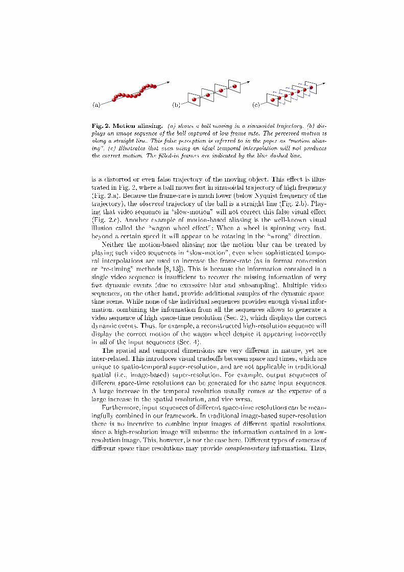
(ii) Motion-Based (Temporal) Aliasing: A more severe problem in video se-quences of fast dynamic events is false visual illusions caused by aliasing in time.Motion aliasing occurs when the trajectory generated by a fast moving object ischaracterized by frequencies which are higher than the frame-rate of the camera(i.e., the temporal sampling rate). When that happens, the high temporal fre-quencies are \folded" into the low temporal frequencies. The observable result

(a) (b) (c)

Fig. 2. Motion aliasing. (a) shows a ball moving in a sinusoidal trajectory. (b) dis-plays an image sequence of the ball captured at low frame-rate. The perceived motion isalong a straight line. This false perception is referred to in the paper as \motion alias-ing". (c) Illustrates that even using an ideal temporal interpolation will not producesthe correct motion. The �lled-in frames are indicated by the blue dashed line.

is a distorted or even false trajectory of the moving object. This e�ect is illus-trated in Fig. 2, where a ball moves fast in sinusoidal trajectory of high frequency(Fig. 2.a). Because the frame-rate is much lower (below Nyquist frequency of thetrajectory), the observed trajectory of the ball is a straight line (Fig. 2.b). Play-ing that video sequence in \slow-motion" will not correct this false visual e�ect(Fig. 2.c). Another example of motion-based aliasing is the well-known visualillusion called the \wagon wheel e�ect": When a wheel is spinning very fast,beyond a certain speed it will appear to be rotating in the \wrong" direction.

Neither the motion-based aliasing nor the motion blur can be treated byplaying such video sequences in \slow-motion", even when sophisticated tempo-ral interpolations are used to increase the frame-rate (as in format conversionor \re-timing" methods [8, 13]). This is because the information contained in asingle video sequence is insuÆcient to recover the missing information of veryfast dynamic events (due to excessive blur and subsampling). Multiple videosequences, on the other hand, provide additional samples of the dynamic space-time scene. While none of the individual sequences provides enough visual infor-mation, combining the information from all the sequences allows to generate avideo sequence of high space-time resolution (Sec. 2), which displays the correctdynamic events. Thus, for example, a reconstructed high-resolution sequence willdisplay the correct motion of the wagon wheel despite it appearing incorrectlyin all of the input sequences (Sec. 4).

The spatial and temporal dimensions are very di�erent in nature, yet areinter-related. This introduces visual tradeo�s between space and times, which areunique to spatio-temporal super-resolution, and are not applicable in traditionalspatial (i.e., image-based) super-resolution. For example, output sequences ofdi�erent space-time resolutions can be generated for the same input sequences.A large increase in the temporal resolution usually comes at the expense of alarge increase in the spatial resolution, and vice versa.

Furthermore, input sequences of di�erent space-time resolutions can be mean-ingfully combined in our framework. In traditional image-based super-resolutionthere is no incentive to combine input images of di�erent spatial resolutions,since a high-resolution image will subsume the information contained in a low-resolution image. This, however, is not the case here. Di�erent types of cameras ofdi�erent space-time resolutions may provide complementary information. Thus,

for example, we can combine information obtained by high-quality still cameras(which have very high spatial-resolution, but extremely low \temporal resolu-tion"), with information obtained by standard video cameras (which have lowspatial-resolution but higher temporal resolution), to obtain an improved videosequence of high spatial and high temporal resolution. These issues and otherspace-time visual tradeo�s are discussed in Sec. 4.

2 Space-Time Super-Resolution

Let S be a dynamic space-time scene. Let fSligni=1 be n video sequences of that

dynamic scene recorded by n di�erent video cameras. The recorded sequenceshave limited spatial and temporal resolution. Their limited resolutions are due tothe space-time imaging process, which can be thought of as a process of blurringfollowed by sampling in time and in space.

The blurring e�ect results of the fact that the color at each pixel in eachframe (referred to as a \space-time point" and marked by the small boxes inFig. 3.a) is an integral (a weighted average) of the colors in a space-time regionin the dynamic scene S (marked by the large pink (bright) and blue (dark) boxesin Fig. 3.a). The temporal extent of this region is determined by the exposure-time of the video camera, and the spatial extent of this region is determinedby the spatial point-spread-function (PSF) of the camera (determined by theproperties of the lens and the detectors [4]).

The sampling process also has a spatial and a temporal components. Thespatial sampling results from the fact that the camera has a discrete and �nitenumber of detectors (the output of each is a single pixel value), and the temporalsampling results from the fact that the camera has a �nite frame-rate resultingin discrete frames (typically 25 frames=sec in PAL cameras and 30 frames=secin NTSC cameras).

The above space-time imaging process inhibits high spatial and high temporalfrequencies of the dynamic scene, resulting in video sequences of low space-timeresolutions. Our objective is to use the information from all these sequences toconstruct a new sequence Sh of high space-time resolution. Such a sequence willhave smaller blurring e�ects and �ner sampling in space and in time, and willthus capture higher space-time frequencies of the dynamic scene S. In particular,it will capture �ne spatial features in the scene and rapid dynamic events whichcannot be captured by the low-resolution sequences.

The recoverable high-resolution information in Sh is limited by its spatialand temporal sampling rate (or discretization) of the space-time volume. Theserates can be di�erent in space and in time. Thus, for example, we can recover asequence Sh of very high spatial resolution but low temporal resolution (e.g., seeFig. 3.b), a sequence of very high temporal resolution but low spatial resolution(e.g., see Fig. 3.c), or a bit of both. These tradeo�s in space-time resolutions andtheir visual e�ects will be discussed in more detail later in Sec. 4.2.

We next model the geometrical relations (Sec. 2.1) and photometric relations(Sec. 2.2) between the unknown high-resolution sequence Sh and the input low-resolution sequences fSl

igni=1.

2.1 The Space-time Coordinate Transformations

In general a space-time dynamic scene is captured by a 4D representation(x; y; z; t). For simplicity, in this paper we deal with dynamic scenes which canbe modeled by a 3D space-time volume (x; y; t) (see in Fig. 3.a). This assumptionis valid if one of the following conditions holds: (i) the scene is planar and thedynamic events occur within this plane, or (ii) the scene is a general dynamic 3Dscene, but the distances between the recording video cameras are small relativeto their distance from the scene. (When the camera centers are very close to eachother, there is no relative 3D parallax.) Under those conditions the dynamicscene can be modeled by a 3D space-time representation.

W.l.o.g., let Sl1 be a \reference" sequence whose axes are aligned with those

of the continuous space-time volume S (the unknown dynamic scene we wish toreconstruct). Sh is a discretization of S with a higher sampling rate than that ofSl1. Thus, we can model the transformation T1 from the space-time coordinate

exposertime

l

(b)

Low resolution input sequences

������������������������

������������������������

������������������������

������������������������

Continuous space-time Different high resolution

(c)

t

t

iS

h

(a)

dynamic scene S discretizations S

nS1

lS

����������X

�����������

�����������

l

X

����

����

X����������

y

yy

�������������������������

�������������������������

�����

�����

Fig. 3. The space-time imaging process. (a) illustrates the space-time continuousscene and two of the low resolution sequences. The large pink (bright) and blue (dark)boxes are the support regions of the space-time blur corresponding to the low resolutionspace-time measurements marked by the respective small boxes. (b,c) show two di�erentpossible discretizations of the space-time volume resulting in two di�erent high resolu-tion output sequences. (b) has a low frame-rate and high spatial resolution, (c) has ahigh frame-rate but low spatial resolution.

system of Sl1 to the space-time coordinate system of Sh by a scaling transfor-

mation (the scaling can be di�erent in time and in space). Let Ti!1 denote thespace-time coordinate transformation from the reference sequence Sl

1 to the i-thlow resolution sequence Sl

i (see below). Then the space-time coordinate transfor-mation of each low-resolution sequence Sl

i is related to that of the high-resolutionsequence Sh by Ti = T1 � Ti!1.

The space-time coordinate transformation between two input sequences(Ti!1) results from the di�erent setting of the di�erent cameras. Atemporal misalignment between two sequences occurs when there is a time-shift(o�set) between them (e.g., if the cameras were not activated simultaneously),or when they di�er in their frame rates (e.g., PAL and NTSC). Such temporalmisalignments can be modeled by a 1-D aÆne transformation in time, and istypically at sub-frame time units. The spatial misalignment between the two se-quences results from the fact that the two cameras have di�erent external andinternal calibration parameters. In our current implementation, as mentionedabove, because the camera centers are assumed to be very close or else the sceneis planar, the spatial transformation can thus be modeled by an inter-camerahomography. We computed these space-time coordinate transformations, usingthe method of [7], which provides high sub-pixel and high sub-frame accuracy.

Note that while the space-time coordinate transformations between the se-quences (fTigni=1) are very simple (a spatial homography and a temporal aÆnetransformation), the motions occurring over time within the dynamic scene canbe very complex. Our space-time super-resolution algorithm does not requireknowledge of these motions, only the knowledge of fTigni=1. It can thus handlevery complex dynamic scenes.

2.2 The Space-Time Imaging Model

As mentioned earlier, the space-time imaging process induces spatial and tem-poral blurring in the low-resolution sequences. The temporal blur in the low-resolution sequence Sl

i is caused by the exposer-time �i of the i-th camera. Thespatial blur in Sl

i is due to the spatial point-spread-function (PSF) of the i-thcamera, which can be approximated by a 2D spatial Gaussian with std �i. (Amethod for estimating the PSF of a camera can be found in [11].)

Let Bi = B(�i;�i;pli)denote the combined space-time blur operator of the i-th

camera corresponding to the low resolution space-time point pli = (xli; yli; t

li). Let

ph = (xh; yh; th) be the corresponding high resolution space-time pointph = Ti(p

li) (p

h is not necessarily an integer grid point of Sh, but is contained inthe continuous space-time volume S). Then the relation between the unknownspace-time values S(ph), and the known low resolution space-time measurementsSli(p

li), can be expressed by:

Sli

�pli�=

�S �Bh

i

�(ph) =

Rx

Ry

Rt

p = (x; y; t) 2 Support(Bhi)

S(p) Bhi (p� ph)dp (1)

where Bhi = Ti(B(�i;�i;pli)

) is a point-dependent space-time blur kernel repre-sented in the high resolution coordinate system. Its support is illustrated by the

large pink (bright) and blue (dark) boxes in Fig. 3.a. To obtain a linear equationin the terms of the discrete unknown values of Sh we used a discrete approxima-tion of Eq. (1). In our implementation we used a non-isotropic approximation inthe temporal dimension, and an isotropic approximation in the spatial dimension(see [6] for a discussion of the di�erent discretization techniques in the contextof image-based super-resolution ). Eq. (1) thus provides a linear equation thatrelates the unknown values in the high resolution sequence Sh to the known lowresolution measurements Sl

i(pli).

When video cameras of di�erent photometric responses are used to producethe input sequences, then a preprocessing step is necessary that histogram-equalizes all the low resolution sequences. This step is required to guaranteeconsistency of the relation in Eq. (1) with respect to all low resolution sequences.

2.3 The Reconstruction Step

Eq. (1) provides a single equation in the high resolution unknowns for each lowresolution space-time measurement. This leads to the following huge system oflinear equations in the unknown high resolution elements of Sh:

A�!h =

�!l (2)

where�!h is a vector containing all the unknown high resolution color values (in

YIQ) of Sh,�!l is a vector containing all the space-time measurements from all

the low resolution sequences, and the matrixA contains the relative contributionsof each high resolution space-time point to each low resolution space-time point,as de�ned by Eq. (1).

When the number of low resolution space-time measurements in�!l is greater

than or equal to the number of space-time points in the high-resolution sequenceSh (i.e., in

�!h ), then there are more equations than unknowns, and Eq. (2) can

be solved using LSQ methods. This, however, implies that a large increase inthe spatial resolution (which requires very �ne spatial sampling in Sh) will comeat the expense of a signi�cant increase in the temporal resolution (which alsorequires �ne temporal sampling in Sh), and vice versa. This is because for a

given set of input low-resolution sequences, the size of�!l is �xed, thus dictating

the number of unknowns in Sh. However, the number high resolution space-time points (unknowns) can be distributed di�erently between space and time,resulting in di�erent space-time resolutions (see 4.2).

Directional space-time regularization. When there is an insuÆcient num-ber of cameras relative to the required improvement in resolution (either in theentire space-time volume, or only in portions of it), then the above set of equa-tions (2) becomes ill-posed. To constrain the solution and provide additionalnumerical stability (as in image-based super-resolution [9, 5]), a space-time reg-ularization term can be added to impose smoothness on the solution Sh in space-time regions which have insuÆcient information. We introduce a directional (or

steerable [14]) space-time regularization term which applies smoothness only indirections where the derivatives are low, and does not smooth across space-time\edges". In other words, we seek

�!h which minimize the following error term:

min�jjA�!h ��!

l jj2 + jjWxLx�!h jj2 + jjWyLy

�!h jj2 + jjWtLt

�!h jj2� (3)

Where Lj (j = x; y; t) is matrix capturing the second-order derivative oper-ator in the direction j, and Wj is a diagonal weight matrix which captures thedegree of desired regularization at each space-time point in the direction j. Theweights in Wj prevent smoothing across space-time \edges". These weights aredetermined by the location, orientation and magnitude of space-time edges, andare approximated using space-time derivatives in the low resolution sequences.

Solving the equations. The optimization problem of Eq. (3) has very largedimensionality. For example, even for a simple case of four low resolution inputsequences, each one-second long (25 frames) and of size 128 � 128 pixels, weget: 1282 � 25� 4 � 1:6� 106 equations from the low resolution measurementsalone (without regularization). Assuming a similar number of high resolutionunknowns poses a severe computational problem. However, matrix A is sparseand local (i.e., all the non zero entries are located in a few diagonals), the systemof equations can be solved using \box relaxation" [15].

3 Examples: Temporal Super-Resolution

Empirical Evaluation. To examine the capabilities of temporal super-resolutionin the presence of strong motion aliasing and strong motion blur, we �rst sim-ulated a sports-like scene with a very fast moving object. We recorded a singlevideo sequence of a basketball bouncing on the ground. To simulate high speed ofthe ball relative to frame-rate and relative to the exposure-time (similar to thoseshown in Fig. 1), we temporally blurred the sequence using a large (9-frame) blurkernel, followed by a large subsampling in time by factor of 30. This process re-sults in a low temporal-resolution sequences of a very fast dynamic event havingan \exposure-time" of about 1

3 of its frame-time. We generated 18 such low res-olution sequences by starting the temporal sub-sampling at arbitrary startingframes. Thus, the input low-resolution sequences are related by non-uniformsub-frame temporal o�sets. Because the original sequence contained 250 frames,each generated low-resolution sequence contains only 7 frames. Three of the 18sequences are presented in Fig 4.a-c. To visually display the event captured ineach of these sequences, we super-imposed all 7 frames in each sequence. Eachball in the super-imposed image represents the location of the ball at a di�erentframe. None of the 18 low resolution sequences captures the correct trajectoryof the ball. Due to the severe motion aliasing, the perceived ball trajectory isroughly a smooth curve, while the true trajectory was more like a cycloid (theball jumped 5 times on the oor). Furthermore, the shape of the ball is com-pletely distorted in all input image frames, due to the strong motion blur.

(a) (b) (c)

(d) (e) (f)

Fig. 4. Temporal super-resolution. We simulated 18 low-resolution video record-ings of a rapidly bouncing ball inducing strong motion blur and motion aliasing (seetext). (a)-(c) Display the dynamic event captured by three representative low-resolutionsequences. These displays were produced by super-position of all 7 frames in each low-resolution sequences. All 18 input sequences contain severe motion aliasing (evidentfrom the falsely perceived curved trajectory of the ball) and strong motion blur (evi-dent from the distorted shapes of the ball). (d) The reconstructed dynamic event ascaptured by the generated high-resolution sequence. The true trajectory of the ball isrecovered, as well as its correct shape. (e) A close-up image of the distorted ball inone of the low resolution frames. (f) A close-up image of the ball at the exact corre-sponding frame in time in the high-resolution output sequence. For color sequences see:www.wisdom.weizmann.ac.il/�vision/SuperRes.html

We applied the super-resolution algorithm of Sec. 2 on these 18 low-resolutioninput sequences, and constructed a high-resolution sequence whose frame-rate is30 times higher than that of the input sequences. (In this case we requested anincrease only in the temporal sampling rate). The reconstructed high-resolutionsequence is shown in Fig. 4.d. This is a super-imposed display of some of thereconstructed frames (every 8'th frame). The true trajectory of the bouncingball has been recovered. Furthermore, Figs. 4(e)-(f) show that this process hassigni�cantly reduced e�ects of motion blur and the true shape of moving ball hasbeen automatically recovered, although no single low resolution frame containsthe true shape of the ball. Note that no estimation of the ball motion was neededto obtain these results. This e�ect is explained in more details in Sec. 4.1.

The above results obtained by temporal super-resolution cannot be obtainedby playing any low-resolution sequence in \slow-motion" due to the strong mo-tion aliasing. Such results cannot be obtained either by interleaving frames from

the 18 input sequences, due to the non-uniform time shifts between the sequencesand due to the severe motion-blur observed in the individual image frames.

A Real Example - The \Wagon-Wheel E�ect". We used four indepen-dent PAL video cameras to record a scene of a fan rotating clock-wise veryfast. The fan rotated faster and faster, until at some stage it exceeded themaximal velocity that can be captured by video frame-rate. As expected, atthat moment all four input sequences display the classical \wagon wheel e�ect"where the fan appears to be falsely rotating backwards (counter clock-wise).We computed the spatial and temporal misalignments between the sequencesat sub-pixel and sub-frame accuracy using [7] (the recovered temporal misalign-ments are displayed in Fig. 5.a-d using a time-bar). We used the super-resolutionmethod of Sec. 2 to increase the temporal resolution by a factor of 3 whilemaintaining the same spatial resolution. The resulting high-resolution sequencedisplays the true forward (clock-wise) motion of the fan, as if recorded by ahigh-speed camera (in this case, 75frames=sec) . Example of a few successiveframes from each low resolution input sequence are shown in Fig.5.a-d for theportion where the fan appears to be rotating counter clock-wise. A few suc-cessive frames from the reconstructed high temporal-resolution sequence corre-sponding to the same time are shown in Fig.5.e, showing the correctly recovered(clock-wise) motion. It is diÆcult to perceive these strong dynamic e�ects viaa static �gure (Fig. 5). We therefore urge the reader to view the video clipsin www.wisdom.weizmann.ac.il/�vision/SuperRes.html where these e�ects arevery vivid . Furthermore, playing the input sequences in \slow-motion" (usingany type of temporal interpolation) will not reduce the perceived false motione�ects.

4 Space-Time Visual Tradeo�s

The spatial and temporal dimensions are very di�erent in nature, yet are inter-related. This introduces visual tradeo�s between space and time, which areunique to spatio-temporal super-resolution, and are not applicable to traditionalspatial (i.e., image-based) super-resolution.

4.1 Temporal Treatment of Spatial Artifacts

When an object moves fast relative to the exposure time of the camera, it inducesobservable motion-blur (e.g., see Fig. 1). The perceived distortion is spatial,however the cause is temporal. We next show that by increasing the temporalresolution we can handle the spatial artifacts caused by motion blur.

Motion blur is caused by the extended temporal blur due to the exposure-time. To decrease e�ects of motion blur we need to decrease the temporal blur,i.e., recover high temporal frequencies. This requires increasing the frame-ratebeyond that of the low resolution input sequences. In fact, to decrease the e�ectof motion blur, the output temporal sampling rate must be increased so that the

(a) (b)

(c) (d)

(e)

Fig. 5. Temporal super-resolution (the \wagon wheel e�ect"). (a)-(d) display3 successive frames from four PAL video recordings of a fan rotating clock-wise. Becausethe fan is rotating very fast (almost 90o between successive frames), the motion aliasinggenerates a false perception of the fan rotating slowly in the opposite direction (counterclock-wise) in all four input sequences. The temporal misalignments between the inputsequences were computed at sub-frame temporal accuracy, and are indicated by theirtime bars. The spatial misalignments between the sequences (e.g., due to di�erencesin zoom and orientation) were modeled by a homography, and computed at sub-pixelaccuracy. (e) shows the reconstructed video sequence in which the temporal resolutionwas increased by a factor of 3. The new frame rate (75 frames

sec) is also indicated by a

time bars. The correct clock-wise motion of the fan is recovered. For color sequencessee: www.wisdom.weizmann.ac.il/�vision/SuperRes.html

distance between the new high resolution temporal samples is smaller than theoriginal exposure time of the low resolution input sequences.

This indeed was the case in the experiment of Fig. 4. Since the simulatedexposure time in the low resolution sequences was 1=3 of frame-time, an increasein temporal sampling rate by a factor> 3 can reduce the motion blur. The largerthe increase the more e�ective the motion deblurring would be. This increase islimited, of course, by the number of input cameras.

A method for treating motion blur in the context of image-based super-resolution was proposed by [2, 12]. However, these methods require a prior seg-mentation of moving objects and the estimation of their motions. These methodswill have diÆculties handling complex motions or motion aliasing. The distortedshape of the object due to strong blur (e.g., Fig. 1) will pose severe problems inmotion estimation. Furthermore, in the presence of motion aliasing, the directionof the estimated motion will not align with the direction of the induced blur.For example, the motion blur in Fig. 4.a-c. is along the true trajectory and not

along the perceived one. In contrast, our approach does not require separationof static and dynamic scene components, nor their motion estimation, thus canhandle very complex scene dynamics. However, we require multiple cameras.

Temporal frequencies in video sequences have very di�erent characteristicsthan spatial frequencies, due to the di�erent characteristics of the temporal andthe spatial blur. The typical support of the spatial blur (PSF) is of a few pixels(�>1 pixel), whereas the exposure time is usually smaller than a single frame-time (� < frame-time). Therefore, if we do not increase the output temporalsampling-rate enough, we will not improve the temporal resolution. In fact, if weincrease the temporal sampling-rate a little but not beyond 1

exposure timeof the

low resolution sequences, we may even introduce additional motion blur.

This dictates the number of input cameras needed for an e�ective decreasein the motion-blur. An example of a case where an insuÆcient increase in thetemporal sampling-rate introduced additional motion-blur is shown in Fig. 6.c3.

4.2 Producing Di�erent Space-Time Outputs

In standard spatial super-resolution the increase in sampling rate is equal inall spatial dimensions. This is necessary in order to maintain the aspect ratioof image pixels, and to prevent distorted-looking images. However, this is notthe case in space-time super-resolution. As explained in Sec. 2, the increase insampling rate in the spatial and temporal dimensions need not be the same.Moreover, increasing the sampling rate in the spatial dimension comes at theexpense of increase in the temporal frame rate, and vice-versa. This is becausethe number of unknowns in the high-resolution space-time volume depends onthe space-time sampling rate, whereas the number of equations provided by thelow resolution measurements remains �xed.

For example, assume that 8 video cameras are used to record a dynamicscene. One can increase the spatial sampling rate alone by a factor of

p8 in x

and y, or increase the temporal frame-rate alone by a factor of 8, or do a bit ofboth: increase the sampling rate by a factor of 2 in all three dimensions. Suchan example is shown in Fig. 6. Fig. 6.a1 displays one of 8 low resolution inputsequences. (Here we used only 4 video cameras, but split them into 8 sequencesof even and odd �elds). Figs. 6.a2 and 6.a3 display two possible outputs. In Fig.6.a2 the increase is by a factor of 8 in the temporal axis with no increase in thespatial axes, and in Fig. 6.a3 the increase is by a factor of 2 in all axes x,y,t. Rows(b) and (c) illustrate the corresponding visual tradeo�s. The \�1�1�8" option(column 2) decreases the motion blur of the moving object (the toothpaste in(c.2)), while the \�2�2�2" option (column 3) improves the spatial resolutionof the static background (b.3), but increases the motion blur of the movingobject (c.3). The latter is because the increase in frame rate was only by factor2 and did not exceed 1

exposure timeof the video camera (see Sec. 4.1). In order to

create a signi�cant improvement in all dimensions, more than 4 video camerasare needed.

a.1 a.2 a.3

b.1 b.2 b.3

c.1 c.2 c.3

Fig. 6. Tradeo�s between spatial and temporal resolution. This �gure comparesthe visual tradeo�s resulting from applying space-time super-resolution with di�erentdiscretization of the space-time volume. (a.1) displays one of eight low-resolution inputsequences of a toothpaste in motion against a static background. (b.1) shows a close-upimage of a static portion of the scene (the writing on the poster), and (c.1) shows adynamic portion of the scene (the toothpaste). Column 2 (a.2, b.2, c.2) displays theresulting spatial and temporal e�ects of applying super-resolution by a factor of 8 intime only. Motion blur of the toothpaste is decreased. Column 3 (a.3, b.3, c.3) displaysthe resulting spatial and temporal e�ects of applying super-resolution by a factor of 2in all three dimensions x; y; t. The spatial resolution of the static portions is increased(see \British" and the yellow line above it in b.3), but the motion blur is also increased(c.3). See text for an explanation of these visual tradeo�s. For color sequences see:www.wisdom.weizmann.ac.il/�vision/SuperRes.html

4.3 Combining Di�erent Space-Time Inputs

So far we assumed that all input sequences were of similar spatial and temporalresolutions. The space-time super-resolution algorithm of Sec. 2 is not restrictedto this case, and can handle input sequences of varying space-time resolutions.Such a case is meaningless in image-based super-resolution, because a high res-olution input image would always contain the information of a low resolution

image. In space-time super-resolution however, this is not the case. One cameramay have high spatial but low temporal resolution, and the other vice-versa.Thus, for example, it is meaningful to combine information from NTSC andPAL video cameras. NTSC has higher temporal resolution than PAL (30f=secvs. 25f=sec), but lower spatial resolution (640�480 pixels vs. 768�576 pixels). Anextreme case of this idea is to combine information from still and video cameras.Such an example is shown in Fig. 7. Two high quality still images of high spatialresolutions (1120�840 pixels) but extremely low \temporal resolution" (the timegap between the two still images was 1.4 sec), were combined with an interlaced(PAL) video sequence using the algorithm of Sec 2. The video sequence has 3times lower spatial resolution (we used �elds of size 384�288 pixels), but a hightemporal resolution (50f=sec). The goal is to construct a new sequence of highspatial and high temporal resolutions (i.e., 1120�840 pixels at 50 images=sec).

The output sequence shown in Fig. 7.c contains the high spatial resolutionfrom the still images (the sharp text) and the high temporal resolution from thevideo sequence (the rotation of the toy dog and the brightening and dimming ofillumination).

In the example of Fig. 7 we used only one input sequence and two still images,thus did not exceed the temporal resolution of the video or the spatial resolutionof the stills. However, when multiple video cameras and multiple still images areused, the number of input measurements will exceed the number of output highresolution unknowns. In such cases the output sequence will exceed the spatialresolution of the still images and temporal resolution of the video sequences.

In Fig. 7 the number of unknowns was signi�cantly larger than the number oflow resolution measurements (the input video and the two still images). Yet, thereconstructed output was of high quality. The reason for this is the following:In video sequences the data is signi�cantly more redundant than in images,due to the additional time axis. This redundancy provides more exibility inapplying physically meaningful directional regularization. In regions that havehigh spatial resolution but small (or no) motion (such as in the sharp textin Fig. 7), strong temporal regularization can be applied without decreasingthe space-time resolution. Similarly, in regions with very fast dynamic changesbut low spatial resolution (such as in the rotating toy in Fig. 7), strong spatialregularization can be employed without degradation in space-time resolution.More generally, because a video sequence has much more data redundancy thanan image has, the use of directional space-time regularization in video-basedsuper-resolution is physically more meaningful and gives rise to recovery of higherspace-time resolution than that obtainable by image-based super-resolution withimage-based regularization.

Acknowledgments

The authors wish to thank Merav Galun & Achi Brandt for their helpful sug-gestions regarding solutions of large scale systems of equations. Special thanksto Ronen Basri & Lihi Zelnik for their useful comments on the paper.

Fig. 7. Combining Still and Video. A dynamic scene of a rotating toy-dog and vary-ing illumination was captured by: (a) A still camera with spatial resolution of 1120�840pixels, and (b) A video camera with 384�288 pixels at 50 f/sec. The video sequence was1:4sec long (70 frames), and the still images were taken 1:4sec apart (together with the�rst and last frames). The algorithm of Sec. 2 is used to generate the high resolutionsequence (c). The output sequence has the spatial dimensions of the still images andthe frame-rate of the video (1120� 840�50). It captures the temporal changes correctly(the rotating toy and the varying illumination), as well the high spatial resolution ofthe still images (the sharp text). Due to lack of space we show only a portion of theimages, but the proportions between video and still are maintained. For color sequencessee: www.wisdom.weizmann.ac.il/�vision/SuperRes.html

References

1. S. Baker and T. Kanade. Limits on super-resolution and how to break them. InCVPR, Hilton Head Island, South Carolina, June 2000.

2. B. Bascle, A. Blake, and A.Zisserman. Motion deblurring and super-resolutionfrom an image sequence. In ECCV, pages 312{320, 1996.

3. S. Borman and R. Stevenson. Spatial resolution enhancement of low-resolution im-age sequences - a comprehensive review with directions for future research. Techni-cal report, Laboratory for Image and Signal Analysis (LISA), University of NotreDame, Notre Dame, July 1998.

4. M. Born and E. Wolf. Principles of Optics. Permagon Press, 1965.5. D. Capel and A. Zisserman. Automated mosaicing with super-resolution zoom. In

CVPR, pages 885{891, June 1998.6. D. Capel and A. Zisserman. Super-resolution enhancement of text image sequences.

In ICPR, pages 600{605, 2000.7. Y. Caspi and M. Irani. A step towards sequence-to-sequence alignment. In CVPR,

pages 682{689, Hilton Head Island, South Carolina, June 2000.8. G. de Haan. Progress in motion estimation for consumer video format conversion.

IEEE Transactions on Consumer Electronics, 46(3):449{459, August 2000.9. M. Elad. Super-resolution reconstruction of images. Ph.D. Thesis, Technion Israel

Institute of Technology, December 1996.10. T.S. Huang and R.Y. Tsai. Multi-frame image restoration and registration. In

Advances in Computer Vision and Image Processing, volume 1, pages 317{339.JAI Press Inc., 1984.

11. M. Irani and S. Peleg. Improving resolution by image registration. CVGIP:GM,53:231{239, May 1991.

12. A. J. Patti, M. I. Sezan, and A. M. Tekalp. Superresolution video reconstructionwith arbitrary sampling lattices and nonzero aperture time. In IEEE Trans. onImage Processing, volume 6, pages 1064{1076, August 1997.

13. REALVIZTM . Retimer. www.realviz.com/products/rt, 2002.14. J. Shin, J. Paik, J. R. Price, and M.A. Abidi. Adaptive regularized image interpo-

lation using data fusion and steerable constraints. In SPIE Visual Communicationsand Image Processing, volume 4310, January 2001.

15. U. Trottenber, C. Oosterlee, and A. Sch�uller. Multigrid. Academic Press, 2000.