incorporating mixed item formats in cat: a … · abstract incorporating mixed item formats in cat:...
TRANSCRIPT
INCORPORATING MIXED ITEM FORMATS IN CAT: A COMPARISON OF SHADOW
TEST AND BIN-STRUCTURED APPROACHES
By
Xin Luo
A DISSERTATION
Submitted to
Michigan State University
in partial fulfillment of the requirements
for the degree of
Measurement and Quantitative Methods – Doctor of Philosophy
2015
ABSTRACT
INCORPORATING MIXED ITEM FORMATS IN CAT: A COMPARISON OF SHADOW
TEST AND BIN-STRUCTURED APPROACHES
By
Xin Luo
Current operational CATs mainly use dichotomous items. However, including
polytomous and set-based items into CAT is attracting growing attention. Few studies have been
conducted to investigate how to assemble a mixed-item-format CAT efficiently. The
requirements for assembling a CAT are often in conflict with each other; the test assembly
approach should advance progress toward all objectives. The shadow test approach (STA) is one
of the most appealing CAT assembly methods as it can handle complex constraints. It is very
flexible and can deal with many constraints simultaneously. However, STA solves the
optimization problem uniquely for each examinee, which may result in some problems in
operational CATs, such as context effects and difficulty in item replacement. These problems
can be partially solved by the bin-structured method, which aims to find a single standardized
solution to divide the item pool and solve the constrained combination optimization problem.
However, though the bin-structured method is promising in future applications, as a relatively
new method, research in bin-structured method is still rare, and none uses mixed-item-format
based CAT. And no study investigates what factors may influence the quality of results from the
bin-structured method.
This study compared the mixed-item-based CAT and dichotomous-item-based CAT to
see whether the mixed CAT had advantages over the dichotomous-item-based CAT and what
challenges it brought. Furthermore, it compared three CAT test assembly approaches, including
STA, combination of STA and bin-structured method, and bin-structured method in context of
CAT containing mixed item formats. The psychometric models used in item pool, item
parameter distribution, test length and imposed test constraints were manipulated to simulate
various real test situations.
The results supported incorporating polytomous items and set-based items into CAT, as
mixed CAT had higher test accuracy and stability than the binary CAT. However, the mixed
CAT had a fairly skewed exposure rate distribution, and further analysis showed that the highly
exposed items were all polytomous-scoring items. Another relevant problem for mixed CAT
was its low item usage efficiency, as a lot of items (mainly dichotomous items) were unused.
This study also supported the application of bin-structured method in mixed CAT as it can
produce equal or even better outcomes than the traditional STA. Meanwhile it can also simplify
the computation involved in CAT, standardize the look of the test, provide good control over the
content sequences in advance, and facilitate item replacement and exposure control.

Copyright by
XIN LUO
2015

v
ACKNOWLEDGMENTS
I am deeply indebted to my academic advisor and dissertation chair, Dr. Mark Reckase,
for providing me the great opportunity to pursue advanced study in MQM, Michigan State
University. I have benefited tremendously from his wisdom, insight and knowledge. I
appreciate his guidance in academics, in my dissertation, and also in my career development.
Without his constant support, encouragement, warm care and help, this work would not have
been possible.
I also would like to express my sincere appreciation to my dissertation committee
members, Dr. Kimberly Maier and Dr. Richard Houang in MQM, MSU, Dr. Joseph Martineau at
Center for Assessment, and Dr. Timothy Davey at ETS, for their superb instructions and
suggestions. Their insightful comments and review help me greatly in the dissertation work.
I am also deeply grateful to Dr. Spyros Konstantopoulos, Dr. Edward Roeber, and
Dr.Tenko Raykov, who have been providing me with support and advice during my doctoral
study. I also thank Dr. Hongyun Liu and Dr. Tao Xin from Beijing Normal University for their
guidance since my undergraduate study.
My gratitude also extends to psychometrics research teams at CTB/McGraw Hill, ETS,
and National Council of State Boards of Nursing for providing me with valuable chances to work
on their research and internship projects. My special thanks would go to Qi Diao, Hao Ren, Ada
Woo, Doyoung Kim, Qian Hong, Xiao Luo, Lixiong Gu, Longjuan Liang, Priya Kannan,
Richard Tannenbaum and Wei He. I also thank Dr. Wang in Qualcomm for his great suggestions
on my work.

vi
I appreciate my friends, Liyang Mao, Keyin Wang, Tingqiao Chen, Chi Chang, Jiahui
Zhang, Emre Gonulates, Shuyi Chen, Wei Li, Xinge Ji, Xuechun Zhou, Unhee Ju, Xi Wang, Fei
Chen, and Huili Liu, for lighting up my life during the past five years. I would like to give
special thanks to Guangwei Sun for his care throughout my doctoral study and contribution to
the editorial work of my dissertation. I also thank my significant friends Wen Guo, Yangbing
Xu and Tong Lu from Beijing Normal University for their immeasurable support. Finally, I
would like to thank my parents and my grandparents for their unquestioning love.
vii
TABLE OF CONTENTS
LIST OF TABLES x
LIST OF FIGURES xi
KEY TO ABBREVIATIONS xvi
Chapter 1: Introduction 1
Chapter 2: Literature Review 4
2.1 Item Format 4
2.1.1 Dichotomous Item 4
2.1.2 Polytomous Items 6
2.1.3 Set-based Items 7
2.2 Introduction to Computerized Adaptive Testing 9
2.2.1 A Brief History of CAT 9
2.2.2 Advantages of CAT 10
2.2.3 Procedure for Administrating a CAT 11
Item Pool 12
Psychometric Model 13
Item Selection Rule 16
Starting Point 20
Scoring Rule 21
Stopping Rule 23
2.3 CAT Assembly Approaches 25
2.3.1 Goals of CAT Assembly 25
2.3.2 Assembly Design in CAT 27
STA 28
Bin-Structured Method 31
Chapter 3: Methods and Procedures 36
3.1 Generate Item Pools 36
3.1.1 Data Source 36
3.1.2 Generate the Original Item Pool 39
3.1.3 Recalibrated Item Pool 41
3.1.4 Nested Difficulty 3PLM Pool 42
3.1.5 Nested Difficulty 2PLM Pool 43
3.1.6 Balanced Item Pool 43
3.1.7 Heterogeneous Testlet Pool 44
3.2 Simulation of CAT Procedures 45
3.2.1 Long Tests 45
Original Pool 45
Nested Difficulty 3PLM Pool 49
viii
Recalibrated Pool 50
Nested Difficulty 2PLM Pool 50
Balanced Item Pool 50
Heterogeneous Testlet Pool 50
3.2.2 Short Tests 51
3.3 Evaluation Criteria 52
3.3.1 Measurement Criteria 52
Conditional Statistics 53
Overall Statistics 53
3.3.2 Content Balance 54
3.3.3 Test Security 54
3.3.4 Item Usage 55
Chapter 4: Results 56
4.1 Research Question 1 56
4.1.1 Measurement Criteria 56
Conditional Result 56
Overall Result 57
4.1.2 Test Security Criteria 57
Item Exposure 57
Overlap Rate 57
4.1.3 Item Usage 57
4.2 Research Question 2 58
4.2.1 Measurement Criteria 58
Conditional Result 58
(1) Conditional Bias 58
(2) Conditional Absolute Bias (CAB) 64
(3) Conditional Standard Error of Measurement (CSEM) 70
(4) Test Information Conditional Standard Error
of Measurement (TCSEM) 76
Overall Result 88
(1) Bias 88
(2) Mean Absolute Bias (MAB) 89
(3) Root Mean Squared Error (RMSE) 89
4.2.2 Content Balance 90
4.2.3 Test Security 90
Distribution of Item Exposure Rate 90
(1) Original Item Pool 90
(2) Nested Difficulty 3PLM Pool 91
(3) Recalibrated Pool 92
(4) Nested Difficulty 2PLM Pool 93
(5) Balanced Pool 94
(6) Heterogeneous Pool 95
Overlap Rate 97
(1) Overall Overlap Rate 97
(2) Conditional Overlap Rate (COR) 98
ix
4.2.4 Item Usage 104
Chapter 5: Summary and Discussion 105
5.1 Summary of This Study 105
5.1.1 Measurement Criteria 105
5.1.2 Content Balance 106
5.1.3 Item Exposure Rate Distribution 106
5.1.4 Item Usage 107
5.2 Discussion of Major Findings 107
5.2.1 Incorporating Polytomous Items into CAT 107
5.2.2 Comparing STA and Bin-Structured Method 108
5.2.3 Developing Bins Properly 110
5.3 Implications and Limitations 113
BIBLIOGRAPHY 116
x
LIST OF TABLES
Table 2.1 Item Parameters for a GPCM Item 19
Table 2.2 An Example for CAT Assembly Using STA (van der Linden & Reese, 1998) 31
Table 2.3 Item Pool (Davey, 2005) 32
Table 2.4 CAT Constraints (Davey, 2005) 33
Table 2.5 An Example for a Template (Davey, 2005) 33
Table 2.6 Dividing Items into Bins (Davey, 2005) 33
Table 2.7 Example of First Five Items Selected (Davey, 2005) 34
Table 3.1 OSSLT Test Specification 38
Table 3.2 Modified Test Specification for Heterogeneous Testlet Pool 51
Table 3.3 Test Specification for 22-Item CAT 52
Table 4.1 Overall Bias of Ability Estimate 89
Table 4.2 Overall Mean Absolute Bias (MAB) 89
Table 4.3 RMSE of Estimate 90
Table 4.4 Number of Items Achieving the Highest Exposure Rate 97
Table 4.5 Overall Overlap Rate 97
Table 4.6 Proportion of Unused Items 104
Table 5.1 Comparing Item Usage of Combination Method in Different Pools 111
xi
LIST OF FIGURES
Figure 2.1 Steps for Administrating a CAT (He, 2010) 12
Figure 2.2 ICCs for 2PLM Items 14
Figure 2.3 ICC for 3PLM Item 15
Figure 2.4 Item Category Response Probability Curves for a = 0.93, b = -1.28,
d = [0, 1.3,1.07, -2.37] 16
Figure 2.5 Information for 2PLM Items 18
Figure 2.6 Item Information for Polytomous Items with GPCM 19
Figure 3.1 Test Information for OSSLT 2015 (English) 37
Figure 3.2 Original Pool Information 40
Figure 3.3 Ability Distribution of English Population (OSSLT, 2005) 41
Figure 3.4 Recalibrated Pool Information 42
Figure 3.5 Balanced Pool Information 44
Figure 3.6 Summary of Six Pools 45
Figure 3.7 Five CAT Simulations in the Original Pool 49
Figure 4.1(a) Conditional Bias for the Original Pool, 44 Items 59
Figure 4.1(b) Conditional Bias for the Nested Difficulty 3PLM Pool, 44 Items 60
Figure 4.1(c) Conditional Bias for the Recalibrated Pool, 44 Items 60
Figure 4.1(d) Conditional Bias for the Nested Difficulty 2PLM Pool, 44 Items 61
Figure 4.1(e) Conditional Bias for the Balanced Pool, 44 Items 61
Figure 4.1(f) Conditional Bias for the Heterogeneous Pool, 44 Items 62
Figure 4.1(g) Conditional Bias for the Original Pool, 22 Items 62
Figure 4.1(h) Conditional Bias for the Nested Difficulty 3PLM Pool, 22 Items 63
xii
Figure 4.1(i) Conditional Bias for the Recalibrated Pool, 22 Items 63
Figure 4.1(j) Conditional Bias for the Nested Difficulty 2PLM Pool, 22 Items 64
Figure 4.1(k) Conditional Bias for the Balanced Pool, 22 Items 64
Figure 4.2(a) Conditional Absolute Bias for the Original Pool, 44 Items 65
Figure 4.2(b) Conditional Absolute Bias for the Nested Difficulty 3PLM Pool, 44 Items 66
Figure 4.2(c) Conditional Absolute Bias for the Recalibrated Pool, 44 Items 66
Figure 4.2(d) Conditional Absolute Bias for the Nested Difficulty 2PLM Pool, 44 Items 67
Figure 4.2(e) Conditional Absolute Bias for the Balanced Pool, 44 Items 67
Figure 4.2(f) Conditional Absolute Bias for the Heterogeneous Pool, 44 Items 68
Figure 4.2(g) Conditional Absolute Bias for the Original Pool, 22 Items 68
Figure 4.2(h) Conditional Absolute Bias for the Nested Difficulty 3PLM Pool, 22 Items 69
Figure 4.2(i) Conditional Absolute Bias for the Recalibrated Pool, 22 Items 69
Figure 4.2(j) Conditional Absolute Bias for the Nested Difficulty 2PLM Pool, 22 Items 70
Figure 4.2(k) Conditional Absolute Bias for the Balanced Pool, 22 Items 70
Figure 4.3(a) Conditional SEM for the Original Pool, 44 Items 71
Figure 4.3(b) Conditional SEM for the Nested Difficulty 3PLM Pool, 44 Items 72
Figure 4.3(c) Conditional SEM for the Recalibrated Pool, 44 Items 72
Figure 4.3(d) Conditional SEM for the Nested Difficulty 2PLM Pool, 44 Items 73
Figure 4.3(e) Conditional SEM for the Balanced Pool, 44 Items 73
Figure 4.3(f) Conditional SEM for the Heterogeneous Pool, 44 Items 74
Figure 4.3(g) Conditional SEM for the Original Pool, 22 Items 74
Figure 4.3(h) Conditional SEM for the Nested Difficulty 3PLM Pool, 22 Items 75
Figure 4.3(i) Conditional SEM for the Recalibrated Pool, 22 Items 75
xiii
Figure 4.3(j) Conditional SEM for the Nested Difficulty 2PLM Pool, 22 Items 76
Figure 4.3(k) Conditional SEM for the Balanced Pool, 22 Items 76
Figure 4.4(a) TCSEM for the Original Pool, 44 Items 78
Figure 4.4(b) TCSEM for the Nested Difficulty 3PLM Pool, 44 Items 78
Figure 4.4(c) TCSEM for the Recalibrated Pool, 44 Items 79
Figure 4.4(d) TCSEM for the Nested Difficulty 2PLM Pool, 44 Items 79
Figure 4.4(e) TCSEM for the Balanced Pool, 44 Items 80
Figure 4.4(f) TCSEM for the Heterogeneous Pool, 44 Items 80
Figure 4.4(g) TCSEM for the Original Pool, 22 Items 81
Figure 4.4(h) TCSEM for the Nested Difficulty 3PLM Pool, 22 Items 81
Figure 4.4(i) TCSEM for the Recalibrated Pool, 22 Items 82
Figure 4.4(j) TCSEM for the Nested Difficulty 2PLM Pool, 22 Items 82
Figure 4.4(k) TCSEM for the Balanced Pool, 22 Items 83
Figure 4.5(a) CTI for the Original Pool, 44 Items 83
Figure 4.5(b) CTI for the Nested Difficulty 3PLM Pool, 44 Items 84
Figure 4.5(c) CTI for the Recalibrated Pool, 44 Items 84
Figure 4.5(d) CTI for the Nested Difficulty 2PLM Pool, 44 Items 85
Figure 4.5(e) CTI for the Balanced Pool, 44 Items 85
Figure 4.5(f) CTI for the Heterogeneous Pool, 44 Items 86
Figure 4.5(g) CTI for the Original Pool, 22 Items 86
Figure 4.5(h) CTI for the Nested Difficulty 3PLM Pool, 22 Items 87
Figure 4.5(i) CTI for the Recalibrated Pool, 22 Items 87
Figure 4.5(j) CTI for the Nested Difficulty 2PLM Pool, 22 Items 88
xiv
Figure 4.5(k) CTI for the Balanced Pool, 22 Items 88
Figure 4.6(a) Exposure Rate Distribution for the Original Pool, 44 Items 91
Figure 4.6(b) Exposure Rate Distribution for the Original Pool, 22 Items 91
Figure 4.7(a) Exposure Rate Distribution for the Nested Difficulty 3PLM Pool, 44 Items 92
Figure 4.7(b) Exposure Rate Distribution for the Nested Difficulty 3PLM Pool, 22 Items 92
Figure 4.8(a) Exposure Rate Distribution for the Recalibrated Pool, 44 Items 93
Figure 4.8(b) Exposure Rate Distribution for the Recalibrated Pool, 22 Items 93
Figure 4.9(a) Exposure Rate Distribution for the Nested Difficulty 2PLM Pool, 44 Items 94
Figure 4.9(b) Exposure Rate Distribution for the Nested Difficulty 2PLM Pool, 22 Items 94
Figure 4.10(a) Exposure Rate Distribution for the Balanced Pool, 44 Items 95
Figure 4.10(b) Exposure Rate Distribution for the Balanced Pool, 22 Items 95
Figure 4.11 Exposure Rate Distribution for the Heterogeneous Pool, 44 Items 96
Figure 4.12(a) COR for the Original Pool, 44 Items 98
Figure 4.12(b) COR for the Nested Difficulty 3PLM Pool, 44 Items 99
Figure 4.12(c) COR for the Recalibrated Pool, 44 Items 99
Figure 4.12(d) COR for the Nested Difficulty 2PLM Pool, 44 Items 100
Figure 4.12(e) COR for the Balanced Pool, 44 Items 100
Figure 4.12(f) COR for the Heterogeneous Pool, 44 Items 101
Figure 4.12(g) COR for the Original Pool, 22 Items 101
Figure 4.12(h) COR for the Nested Difficulty 3PLM Pool, 22 Items 102
Figure 4.12(i) COR for the Recalibrated Pool, 22 Items 102
Figure 4.12(j) COR for the Nested Difficulty 2PLM Pool, 22 Items 103
Figure 4.12(k) COR for the Balanced Pool, 22 Items 103
xv
Figure 5.1 Distribution of Item Information at =-1 in Recalibrated Pool 112
Figure 5.2 Distribution of Item Information at =-1 in Nested Difficulty 3PLM Pool 112
xvi
KEY TO ABBREVIATIONS
2PLM: Two-Parameter Logistic Model
3PLM: Three-Parameter Logistic Model
ASVAB: Armed Services Vocational Aptitude Battery
CAB: Conditional Absolute Bias
CAT: Computerized Adaptive Testing
CB: Conditional Bias
CCAT: Constrained Computerized Adaptive Testing
CSEM: Conditional Standard Error of Measurement
CTI: Conditional Test Information
CTT: Classical Test Theory
EAP: Expected a Posteriori
EQAO: Education Quality and Accountability Office
GMAT: Graduate Management Admission Test
GPCM: Generalized Partial Credit Model
GRE: Graduate Record Exam
ICC: Item Characteristic Curve
IRT: Item Response Theory
MAB: Mean Absolute Bias
MAP: Maximum a Posteriori
MC: Multiple-Choice Item
MCCAT: Modified Constrained Computerized Adaptive Testing

xvii
MI: Maximum Information
MLE: Maximum Likelihood Estimation
MML: Marginal Maximum Likelihood
MMM: Modified Multinomial Model
MPI: Maximum Priority Index
NAEP: National Assessment of Educational Progress
NCLEX: Council Licensure Examination for Registered Nurses
OSSD: Ontario Secondary School Diploma
OSSLT: Ontario Secondary School Literacy Test
RMSE: Root-Mean-Standard-Error
SBAC: Smarter Balanced Assessment Consortium
SEM: Standard Errors of Measurement
STA: Shadow Test Approach
TCSEM: Conditional Standard Error of Measurement Obtained from the Test Information
TOEFL: Test of English as a Foreign Language
WLE: Weighed Likelihood Estimation
WDA: Weighted Deviation Algorithm
WPM: Weighted Penalty Model
1
Chapter 1: Introduction
The merits of computerized adaptive testing (CAT) have been widely acknowledged.
Compared with traditional linear tests, CAT adaptively selects items suitable to improve the
examinee’s current ability estimate, and can improve the measurement precision and test
efficiency. Meanwhile it facilitates instant score reporting and enables the test to adopt items of
various types (Wainer, 2000; Weiss & Schleisman, 1999). Over the past decades CAT has been
successfully applied to several large-scale testing programs, such as GRE, GMAT, and TOEFL.
Although current operational CATs mainly consist of dichotomous items, including polytomous
and set-based items into CATs is attracting growing attention. Compared with dichotomous
items, polytomous items and set-based items can provide more item information, and are more
appropriate to measure advanced cognitive activities. Meanwhile the dichotomous items still
have significant values because they can elicit more evidences for examinees’ ability within
limited testing time, and the scoring is more convenient. The prospects of combining
dichotomous, polytomous and set-based items in CAT programs are promising (Parshall, Davey,
& Pashley, 2002; SBAC, 2012), but few studies have been conducted to investigate how to
assemble a mixed-item-format CAT efficiently.
Generally there are three requirements for assembling a CAT (Davey, 2005). The first is
to measure each student’s ability accurately with as few items as possible. The main benefit of
CAT in improving test efficiency derives from the completion of this goal. The second is to
guarantee each test can fulfill the pre-determined content specifications. This is driven by the
demand for enhancing test validity. The third is to avoid item over-exposure and ensure test
security. Exposure control is important in ensuring the test fairness, and also in reducing the cost
in item pool development as the item replacement is often costly. Since an item is usually
2
required to go through a complicated development and review procedure before it is considered
as qualified to be used (Gu, 2007), how to avoid the over-exposure problem and reduce unused
items is worthy of research. These requirements are always in conflict with one another; an
optimal solution which can best advance progress toward all objectives is desired in test
assembly.
Currently different CAT assembly approaches have been developed to find the
combinations of items which can measure the target trait accurately while satisfying all test
constraints. The shadow test approach (STA) is one of the most appealing methods as it can
handle complex constraints (van der Linden & Reese, 1998). The goal of STA is to optimize an
objective function (e.g., test information) under a set of constraints. In contrast to other
approaches, the STA uses binary linear integer programming to assemble a full-size test (i.e., the
shadow test) which can provide accurate measurement while satisfying all the test constraints
before selecting each item; then the item is selected from this shadow test instead from the entire
pool.
As most of the conventional CAT assembly methods, one drawback of the STA is that
the sequence in which items appear is not predictable and varies across examines, which may
lead to context effects (Davey, 2005). Another problem resulted from the unpredictable item
administration is that the decisions made in early stage may rule out items which are important in
later stage, and consequently no feasible solution can be obtained. In addition, changing a
handful of items may influence the performance of the whole pool (Davey, 2005), which makes
item replacement and exposure control difficult. An approach named the “bin-structured method”
was proposed (Davey, 2005) to attack these problems in CAT assembly. Instead of building
totally individualized tests, the bin-structured applies a single solution to partition the item pool
3
to non-overlapping bins. The items in a given bin are interchangeable in terms of test
construction rules (e.g., content area). The test is assembled by selecting one item from each bin,
and therefore the number of bins is the same as the test length. Within this general solution of
partitioning the item pool, a further variety of specific item combinations are provided for item
selection, which makes the bin-structured method no less adaptive than the STA.
Considering the recent trend to incorporate polytomous items and set-based items in
applications of computerized adaptive testing (CAT), and the lack of research into the delivery of
a CAT consisting of mixed item formats, this study investigated the features of mixed CAT and
how to assemble a mixed CAT efficiently, and therefore has important practical and theoretical
implications. Specifically, the following two research objectives were addressed in this study:
1. Compare the mixed-item-based CAT and dichotomous-item-based CAT to see whether
the mixed CAT has advantages over the dichotomous-item-based CAT and what challenges it
brings (e.g., high exposure rate of the polytomous items).
2. Compare a highly individualized test assembly design (specifically, STA) to a bin-
structured approach in the context of CAT containing mixed item formats, in a variety of item
pools with different psychometric models and item parameter distributions. The test length and
imposed test constraints were also manipulated to simulate various real test situations to
investigate how the results vary.
4
Chapter 2: Literature Review
This chapter consists of three sections. First, three item formats involved in this study
(i.e. dichotomous items, polytomous items and testlets) are defined and their advantages and
disadvantages are compared. Second, a brief introduction to computerized adaptive testing
(CAT) is presented, including the history and development, the advantages, and the elements of
CAT. The third section provides a review of several current CAT assembly methods, with the
focus on the methods investigated in this research, i.e., shadow test and bin-structured method.
2.1 Item Format
In most of the current educational tests, items can be classified into two general
categories: discrete items, and set-based items (van der Linden, 2000). Discrete items are
independent of each other and can be further classified as dichotomous items or polytomous
items. Set-based items refer to a set of items related to a common stimulus; items are often
related to each other in some way. Previous research explored the differences between these
item formats in cognitive abilities and skills they can measure, content coverage, reliability,
validity, scoring efficiency, etc. (Cao, 2007). Some major differences are discussed below.
2.1.1 Dichotomous Item
Here is a question from NAEP Grade 4 Science test (NAEP, 2015):
A thermometer shows that the outside air temperature is colder than the temperature at
which water turns to ice. However, ice on the sidewalk melts. What probably caused this?
A. The air heating the sidewalk
B. The sidewalk reflecting sunlight into the air
C. The wind causing the ice on the sidewalk to melt
D. The sunlight making the sidewalk warmer than the air
5
This is a typical dichotomous item, as only option D is regarded as the correct answer
though four choices are provided. Dichotomous items refer to items with only two score
categories, e.g., correct (scored as 1) or incorrect (scored as 0; Lord, 1958). Dichotomous items
are widely used in educational testing and psychology assessment. For example, multiple-choice
items (MC) with only one correct answer or questions from a personality inventory are often
scored dichotomously. Dichotomous items have come to dominate the research and application
in CAT for several reasons: an examinee can answer many dichotomous items in a short time
period, which allows the test to cover a broad range of content and to extract a representative
sample of the examinee’s skills and knowledge (Linn, 1995; Livingston & Rupp, 2004); the
scoring for dichotomous items is objective, fast, convenient, and inexpensive; and, several item
selection algorithms have been proved to be effective in dichotomous-item-based CAT (Chang &
Ying, 1996). However, some dichotomous items like MC are more likely to be influenced by
test-wiseness and guessing (Burton, 2001; Oosterhof, 1996), and may result in overestimated
scores. For example, examinees could rule out some alternatives without knowing which one is
the correct answer. In this case the validity of the test will be compromised. Furthermore,
dichotomous items are not optimal for evoking complex cognitive activities. Although some
studies indicate that well-designed dichotomous items can also elicit evidence for complex
cognitive abilities (Haladyna, 1994; Hamilton, Nussbaum, & Snow, 1997), the spectrum of
abilities that can be reached by dichotomous items is still constrained by their nature (Martinez,
1999). Some cognitive activities involving generating creative or divergent production are hard
to be assessed by dichotomous items (Martinez, 1999). If a test intending to evaluate complex
constructs only adopts dichotomous items, the construct might be under-represented, and the
validity will be questionable (Messick, 1995). Therefore, to measure higher-order cognitive
6
functioning, more complex item formats like polytomous items or set-based tests are needed
(Zhou, 2012), as these items can assess a broader range of cognitive ability.
2.1.2 Polytomous Items
The item below is from Education Quality and Accountability Office (EQAO) Grade 4
Writing test (EQAO, 2014):
Your class has agreed to do some volunteer work in your school this year. Each student
can work in an area of his or her choosing. Write a detailed paragraph explaining what you
choose to do and why.
In contrast to being scored simply as correct or incorrect, the response to this item is
evaluated using a 6-point scale, where 0 means the response is almost not readable, and 5
indicates high writing proficiency. Items scored in more than two categories are referred to as
polytomous items (Muraki, 1992). Constructed-response items, ordered response items, and
multiple-response items often adopt polytomous scoring. Over the past few decades, there is an
increasing demand for incorporating polytomous items into a CAT (van Rijn, Eggen, Hemker, &
Sanders, 2002), and several item selection strategies developed for polytomous CAT also
contribute to the growing popularity of polytomous-item-based CAT (Choi & Swartz, 2009).
Moreover, although the scoring for polytomous item requires detailed rubrics, and is more
complicated and time-consuming than dichotomous items, the advance in automated scoring
improves the feasibility of including polytomous item in CAT (Attali & Burstein, 2006).
Compared to dichotomous items, polytomous items can provide more information about
the trait level of an examinee (Bock, 1972; Drasgow, Levine, Williams, McLaughlin, & Candell,
1989; Thissen & Steinberg, 1984). Furthermore, they can reflect the association among
knowledge and skills, and measure more complex constructs (Bock, 1972), which may not be
7
easily accomplished by simple dichotomous items such as MC or true/false items. Another
advantage of polytomous items over dichotomous items is that they may trace students’
cognitive activities by recording their solution processes, and provide diagnostic information and
facilitate educational instruction (Lukhele, Thissen, & Wainer, 1994; Martinez, 1999). Besides,
the developments in computer technology facilitate the delivery of innovative items, and
innovative item formats often require polytomous scoring, which also makes polytomous items
more appealing in CAT (van der Linden & Glas, 2000).
However, though the use of polytomous items shows promise for measuring complex
ability and obtaining higher measurement precision, developing and using these items may be
costly and time-consuming. Hence, how to avoid over-exposure of these items is a main
objective of CAT assembly and will be discussed in this research.
2.1.3 Set-based Items
Set-based items, also known as testlets, refer to items grouped into clusters around a
common stimulus (Wainer & Kiely, 1987). For example, in a reading test, it’s common that a
reading passage is followed by several questions related to this passage. Questions associated
with the same reading passage are regarded as a testlet. The items within a testlet usually share
some similarities and therefore demonstrate some homogeneity in content or assessed skills, and
are not independent (Wainer, Bradlow, & Wang, 2007). Set-based items allow for more
complicated, interrelated sets of items, and make use of the examinee’s time efficiently, as they
require less time in reading and understanding materials. Set-based items also make the task
more realistic, as many real-world tasks require solving related problems in a stepwise fashion;
therefore including set-based items could potentially improve construct validity. And similar to
polytomous items, set-based items are also appropriate to measure higher-level skills. For

8
instance, the development of performance-based testing is a great spur to the popularity of set-
based items, as set-based items may help to elucidate more information on complex cognitions
required in performance tests (van der Linden, 2000).
Assembling set-based tests is much more complex than building discrete-item-based tests,
as the specifications for set-based tests are more complicated (van der Linden, 2000).
Constraints for set-based tests may involve at least four levels: individual items, stimuli, item
sets, and the entire tests (van der Linden, 2000). Several studies have investigated how to
assemble set-based tests, but mainly in linear form (van der Linden, 2000). Assembly methods
proposed in previous research include: (1) use separate decision variables to select item and
stimuli simultaneously (van der Linden, 1992); (2) simultaneously select pivot items; in this
method, the items which best represent the stimuli are defined as the pivot items and are drawn
for administration (van der Linden, 2000); (3) power set approach. The basic idea of this
approach is that suppose an item set contains n items, and then the set will have at most 2n-1
different subsets. The test can be assembled using separate decision variables for whether to
include each subset in the test; (4) two-stage selection, where Stage 1 picks an item set and Stage
2 selects items from the selected sets; and (5) select all items in a set; in this method, if one
stimulus is selected, all the items related with it will be included in the test, and no within-set
selection is performed. Davey (2005) suggests using the entire set rather than item as the unit for
item selection, as the latter strategy complicates determining and picking the “best” set. Other
issues related with using set-based items are how to develop high quality items, and what should
be done to deal with the inter-correlation among items within a same set.
When the violation of local independence is serious, generally two ways can be used to
model the set-based items: the first is to fit a testlet response model (Wainer et al., 2007), and the
9
second is to treat the testlet as a polytomous item (Cook, Dodd, & Fitzpatrick, 1998). In this
study, the testlet will be treated as an intact polytomous-scored unit in item selection and no
within-testlet adaption is conducted. However, although adopting polytomous scoring, the set-
based item is still regarded as a unique item format different from the polytomous item when
developing the blueprint and selecting items in CAT. It also should be noted that a testlet may
cover several content areas or cognitive skills simultaneously, which introduces within-testlet
heterogeneity and distinguishes testlet-based item from polytomous item.
In summary, one single item format cannot be better than another in all aspects, and a
mixed-format test may concatenate their strengths while compensating for some weaknesses, and
achieve broad content coverage, high reliability and validity, efficient scoring, and integrated
measurement scope of high-level cognitive abilities. In conclusion, a test with a mixture of
different item formats may provide more efficient, valid and comprehensive measurement. This
trend is more obvious in CAT, where polytomous items and set-based items hold promises for
future application in CAT as computer provides various options for using innovative items, while
dichotomous items continue to have value.
2.2 Introduction to Computerized Adaptive Testing
Computerized adaptive testing (CAT) has been widely used in educational and
psychological testing. CAT assembles individualized tests by administering items suitable for
measuring the examinee’s ability, and therefore shortens the test length without losing the test
precision.
2.2.1 A Brief History of CAT
Although CAT only has begun to attract attention in educational practice since mid-1990s,
the idea of adaptive testing is much older. The initial attempt at an adaptive test derives from
10
Binet’s and Simon’s intelligence test. They tested students with a subset of items targeted at
their approximate ability instead of using the whole test. If a student answered these items
correctly, harder items would then be administered; otherwise easier items would be
administered (Binet & Simon, 1905). In this way, adaptive tests are able to eliminate items with
inappropriate difficulty, thereby increasing test efficiency and measurement accuracy. Other
early adaptive testing includes Lord's flexilevel testing (1971) and Weiss' stradaptive test (1973).
In these methods, each difficulty level has several item sets, and whether an examinee get a
harder or easier set depends on his or her performance on the previous set.
Since 1990s, the application of computers facilitates further advancement in adaptive
testing (Mills & Stocking, 1996). Currently adaptive testing has been successfully applied to
many large-scale assessments, such as the Council Licensure Examination for Registered Nurses
(NCLEX), Armed Services Vocational Aptitude Battery (ASVAB), Graduate Record
Examination (GRE) and Smarter Balanced Assessment Consortium (SBAC). The popularity of
computerized adaptive testing (i.e., CAT) mainly increases due to two factors: one is the
progress of psychometrics theories, such as Item Response Theory (IRT; Lord, 1980; Weiss,
1978); and the other is the rapid development of computer technology facilitating instantaneous
computation (van der Linden & Glas, 2000; He, 2010).
2.2.2 Advantages of CAT
The advantages of CAT over linear tests have been well documented (Gu, 2007; Wainer,
2000; Way, 1998). First, by giving examinees items with appropriate difficulty, CAT decreases
test length, increases test efficiency, and reduces examinee fatigue (Chang, 2004). While linear
tests usually cannot provide enough information for students at the ends of the ability continuum,
a CAT can maintain measurement precision across the whole ability continuum (Chang, 2004).
11
Second, the removal of poorly performing items is easier in individualized CAT; and an item
with undesirable psychometrics characteristics (e.g., with high differential item functioning) will
only affect some of the examinees. Even for these examinees, as long as sufficient items are
administered, the final estimate of their ability will converge to their true ability value (i.e., the
ability value in theory). This self-correcting feature of CAT would likely decrease the impact of
small numbers of poorly developed items and avoid severely biased estimates of student ability
(Gu, 2007). Third, different examinees receive different items in CAT; the individualized “test
form” helps reduce cheating. Fourth, CAT facilitates calculation of scores without a time lag,
and therefore allows for immediate score delivery, which is very appealing to test-takers (van der
Linden, 2010). Fifth, each examinee can control their testing pace, which reduces test anxiety
and makes the test more flexible. Finally, the application of computer has the potential to use a
variety of novel item formats such as items containing interactive video, and may improve the
test validity. These attractive features lead to extensive use of CAT in educational and
psychological assessments. To examine how CAT improves test efficiency, the section below
demonstrates the process of administration a CAT.
2.2.3 Procedure for Administrating a CAT
As CATs proceed in an iterative way, the design and administration of a CAT is
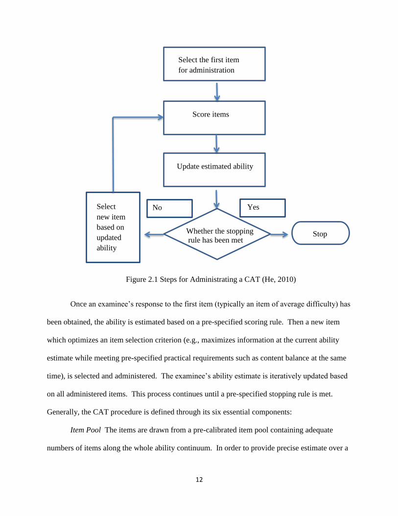
significantly different from a linear test. Figure 2.1 (He, 2010) provides a good illustration of the
adaptive nature of CAT.
12
Figure 2.1 Steps for Administrating a CAT (He, 2010)
Once an examinee’s response to the first item (typically an item of average difficulty) has
been obtained, the ability is estimated based on a pre-specified scoring rule. Then a new item
which optimizes an item selection criterion (e.g., maximizes information at the current ability
estimate while meeting pre-specified practical requirements such as content balance at the same
time), is selected and administered. The examinee’s ability estimate is iteratively updated based
on all administered items. This process continues until a pre-specified stopping rule is met.
Generally, the CAT procedure is defined through its six essential components:
Item Pool The items are drawn from a pre-calibrated item pool containing adequate
numbers of items along the whole ability continuum. In order to provide precise estimate over a
Score items
Update estimated ability
Select the first item
for administration
No Yes Select
new item
based on
updated
ability
estimate
Whether the stopping
rule has been met Stop
13
broad range of ability, a large item pool size is suggested (Luecht, 1998; Patsula & Steffan,
1997). Meanwhile, though exposure control and content balance are not necessary parts of CAT,
they are often required since they can improve test security and validity. The requirements for
having sufficient items in each content area, avoiding item over-exposure to enhance security,
and item retirement reinforce the need for large pool size. Considering the cost and effort to
develop and maintain an item pool, how to maintain a reasonable level of item exposure and
facilitate item replacement is important. The method involved in this study, i.e., the bin-
structured method, may throw some light on this issue.
Psychometric Model The psychometric model is typically based on IRT. IRT
encompasses a set of models connecting the probability of answering an item correctly with an
unobservable and hypothesized trait (i.e., a latent trait). This study is conducted within the
framework of unidimensional IRT (Lord, 1980) and entails three basic assumptions: (1) the test
only measures along one latent trait; (2) the item responses on different items are independent
given the latent trait value; and (3) a monotonically increasing function can be specified to
represent the interaction between items and the person trait, i.e., the probability of getting an
item increases as the latent trait increases.
These three assumptions outline a general class of unidimensional IRT models (Reckase,
2009). Based on the number of scored responses, these models can be divided into two families:
dichotomous model (e.g., one-, two-, and three-parameter logistic model; Lord, 1980), and
polytomous models (e.g., the nominal response model, Bock, 1972; the partial credit model,
Maters, 1982; the generalized partial credit model, Muraki, 1992; and the graded response model,
Samejima, 1969). In this study, two-parameter logistic model (2PLM) and three-parameter
model (3PLM) are used for dichotomous items, as the original dichotomous item calibration was
14
conducted with 3PLM with fixed a- and c-parameter (OSSLT, 2014), and 2PLM is widely used
in modeling dichotomous items in operational CAT. The generalized partial credit model
(GPCM) is used for polytomous items and set-based items since the original data used in this
study adopted GPCM to calibrate polytomous items.
The 2PLM is defined as:
Pj (θ) = ( )
( ) (2.1)
where θ is the person (ability) parameter, aj is the discrimination of item j, bj is difficulty, D is a
scaling constant to approximate the normal ogive model, and Pj (θ) is the probability of getting a
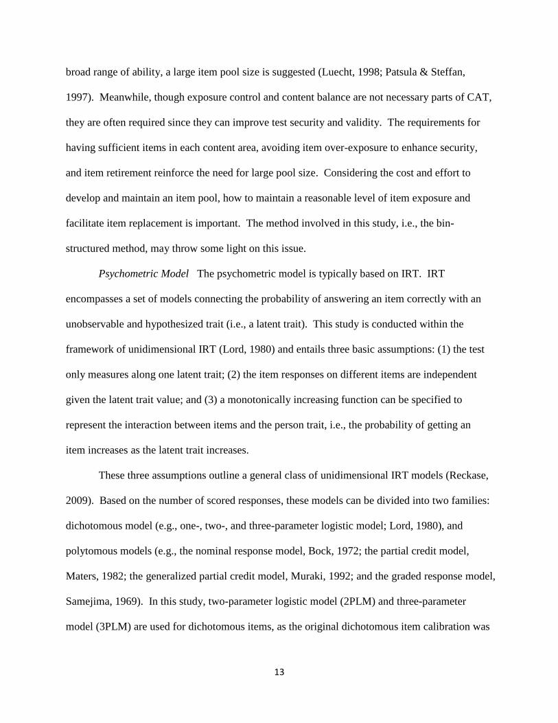
correct response (Lord, 1980). Figure 2.2 shows the item characteristic curve (ICC) for three
two-parameter items.
Figure 2.2 ICCs for 2PLM Items
In 2PLM, an examinee with very low proficiency has little chance to answer a difficult
item correctly. However in real tests, especially in multiple-choice based tests, even low
proficiency examinees still have a notable probability of responding correctly to an item. In
response to this phenomenon, the 3PLM includes a lower asymptote parameter c, which is also
-4 -3 -2 -1 0 1 2 3 40
0.1
0.2
0.3
0.4
0.5
0.6
0.7
0.8
0.9
1
Pro
bab
ility
of G
ettin
g C
orr
ect R
espo
nse
a=1 b=-0.5
a=1.2 b=-0.5
a=1.2 b=0.5
15
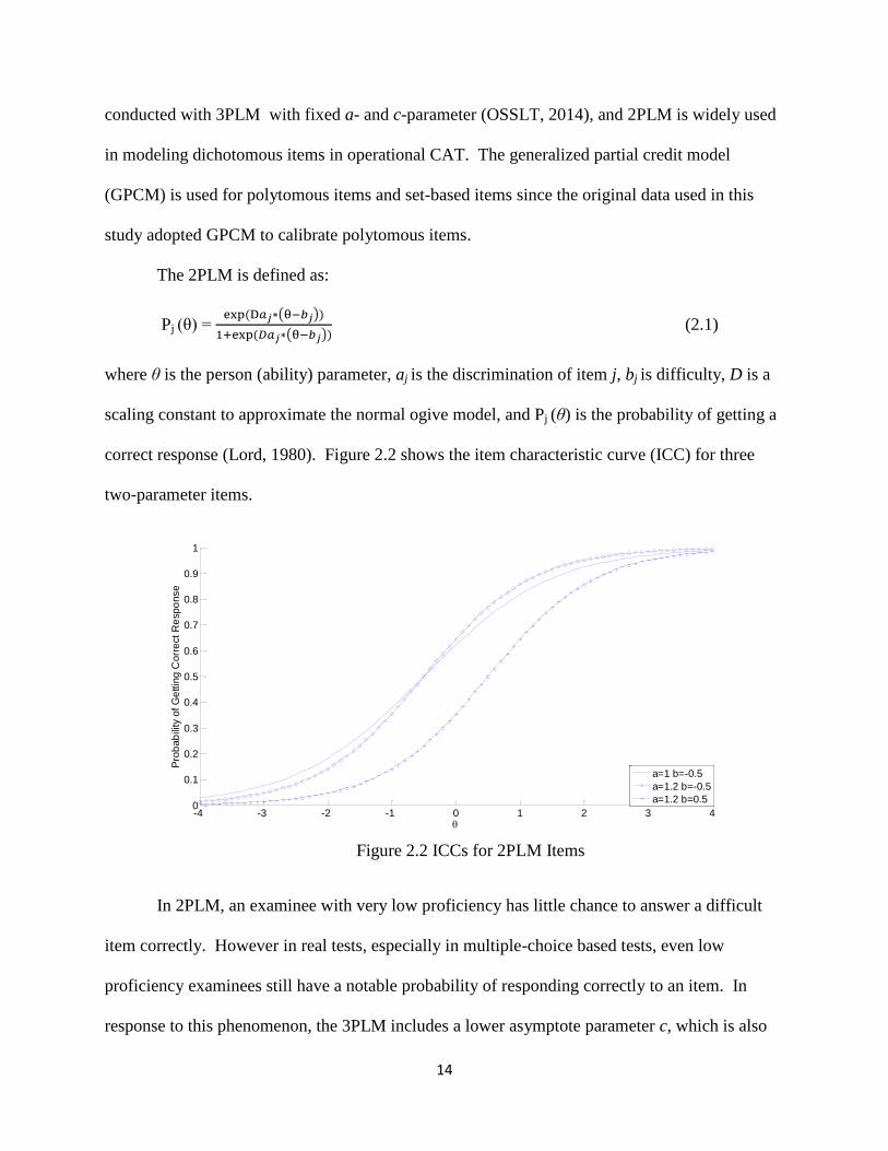
known as guessing parameter or the pseudo chance parameter, indicating the probability of
yielding a correct response by an examinee of extremely low ability. The 3PLM is defined as:
Pj (θ) = ( ) ( )
( ) (2.2)
where is the a lower asymptote parameter for item j, and all the other notations have the same
meaning as 2PLM. Figure 2.3 shows an item modeled with 3PLM. The lower end of the ICC is
not 0; instead, it’s equal to the lower asymptote parameter.
Figure 2.3 ICC for 3PLM Item
The GPCM is an extension of the 2PLM to polytomous items (Davis, 2004). GPCM is
appropriate to model the item which comprises a series of ordered problem solving steps and
examinees can get partial credit for completing a step. For example, solving the math problem
below needs two steps:
2+3*4=?
The first step is to get 3*4=12, and the second step is 2+12=14. The examinee can get
partial score if they complete either step, and get full score if they get both steps correct.
The GPCM is defined as:
-4 -3 -2 -1 0 1 2 3 40
0.1
0.2
0.3
0.4
0.5
0.6
0.7
0.8
0.9
1
Pro
bab
ility
of G
ettin
g C
orr
ect R
espo
nse
a=1 b=0.5,c=0.2
16
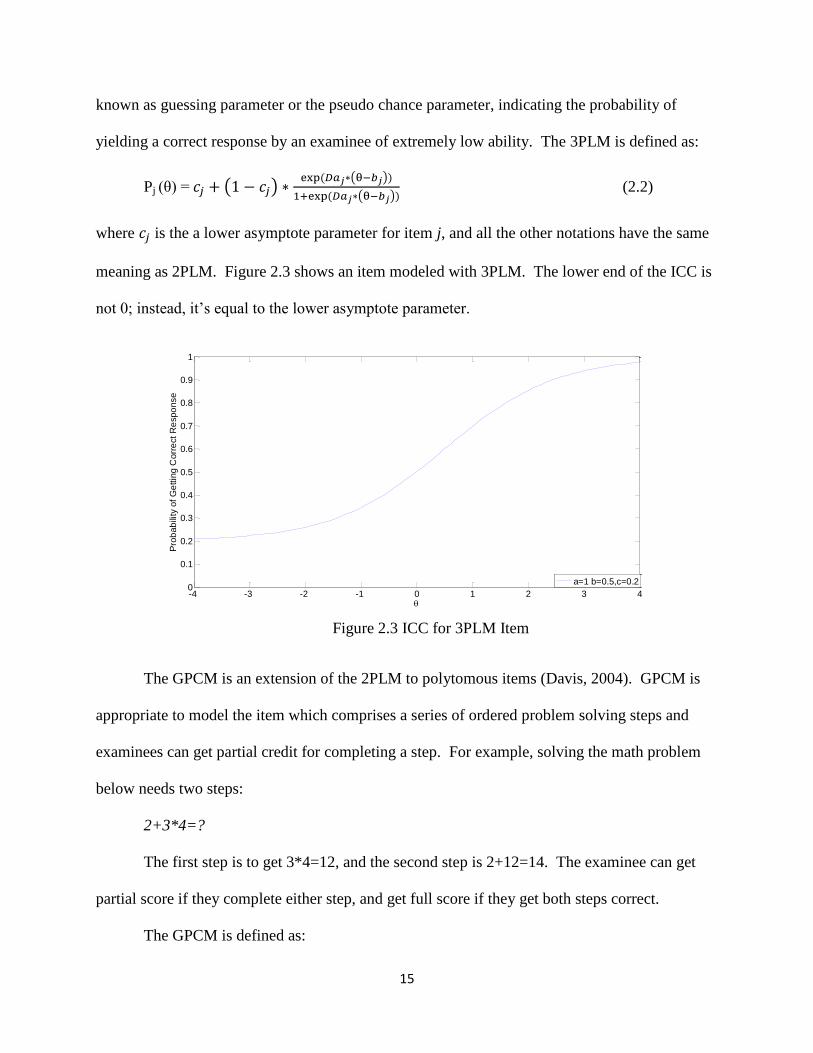
Pjk (θ) = ∑
∑ ∑
(2.3)
where Pjk is the probability of getting score k for item j, θ is the person ability, D is the scaling
constant fixed at 1.7 to approximate the normal ogive model, is the discrimination parameter,
is the overall item difficulty parameter, is the highest scoring category for item j, and is
category threshold parameter. To resolve the indeterminacies in item estimation, for each item
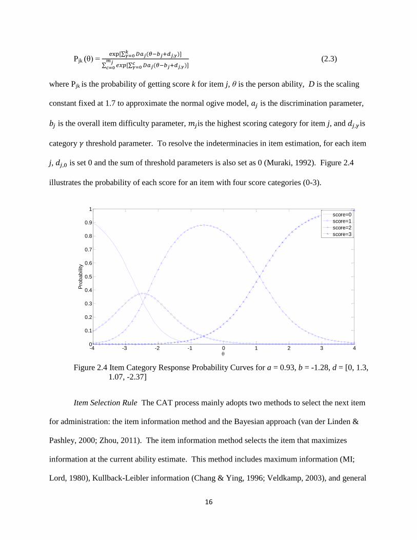
j, is set 0 and the sum of threshold parameters is also set as 0 (Muraki, 1992). Figure 2.4
illustrates the probability of each score for an item with four score categories (0-3).
Figure 2.4 Item Category Response Probability Curves for a = 0.93, b = -1.28, d = [0, 1.3,
1.07, -2.37]
Item Selection Rule The CAT process mainly adopts two methods to select the next item
for administration: the item information method and the Bayesian approach (van der Linden &
Pashley, 2000; Zhou, 2011). The item information method selects the item that maximizes
information at the current ability estimate. This method includes maximum information (MI;
Lord, 1980), Kullback-Leibler information (Chang & Ying, 1996; Veldkamp, 2003), and general
-4 -3 -2 -1 0 1 2 3 40
0.1
0.2
0.3
0.4
0.5
0.6
0.7
0.8
0.9
1
Pro
bab
ility
score=0
score=1
score=2
score=3
17
weighted information method (Veerkamp & Berger, 1997; Choi &Swartz, 2009; van Rijn, Eggen,
Hemker, & Sanders, 2002). The Bayesian method incorporates a weight function of a prior
ability distribution into the information function to form the posterior distribution. This method
comprises maximum posterior weighted information (van der Linden, 1998), maximum expected
information (van der Linden, 1998), and the minimum expected posterior variance method (van
der Linden, 1998). Various studies have compared the performance of different item selection
methods under a number of IRT models, test lengths, and other CAT constraints (Veldkamp,
2003; van Rijn et al., 2002; Ho, 2010), and found no significant difference between MI and other
item selection methods in general. Therefore, MI is used in this study as its computation is
easier.
MI selects the item with maximum Fisher information at the current ability estimate.
Fisher information (also simply named as information) indicates how much information that an
observable random variable (i.e., the response to an item) has about the unknown parameter θ on
which the probability of the random variable relies (Pratt, 1976). For a given dichotomous item j,
information is:
Ij (θ) =
(2.4)
where denotes the derivative of the item response function with respect to θ.
Specifically, for 2PLM, the item information is:
Ij (θ) = . (2.5)
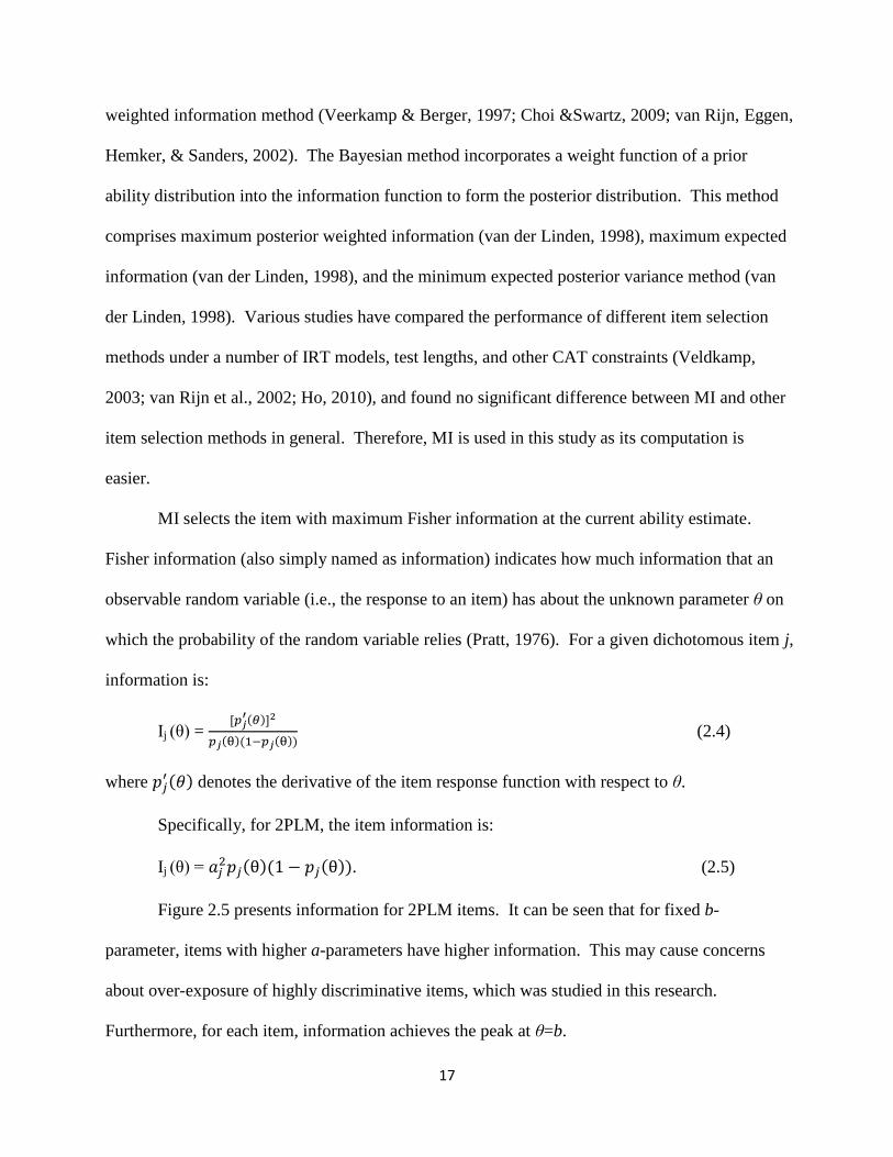
Figure 2.5 presents information for 2PLM items. It can be seen that for fixed b-
parameter, items with higher a-parameters have higher information. This may cause concerns
about over-exposure of highly discriminative items, which was studied in this research.
Furthermore, for each item, information achieves the peak at θ=b.
18
Figure 2.5 Information for 2PLM Items
For the 3PLM in function 2.2, the information is:
Ij (θ) =
( ) (2.6)
where Lj is equal to ( ) (see Hambleton, Swaminathan, & Rogers, 1991; Lord, 1980).
For the GPCM, the item information given ability θ is:
Ij (θ) = ∑
∑
(2.7)
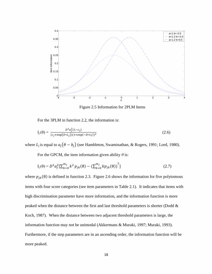
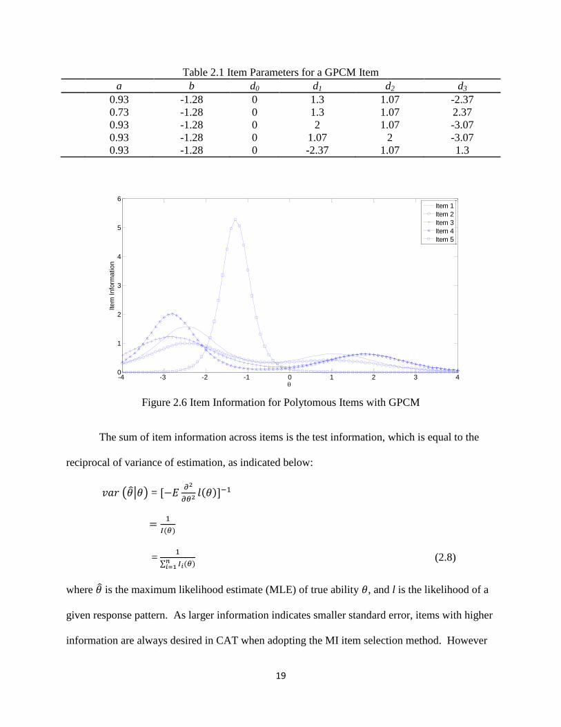
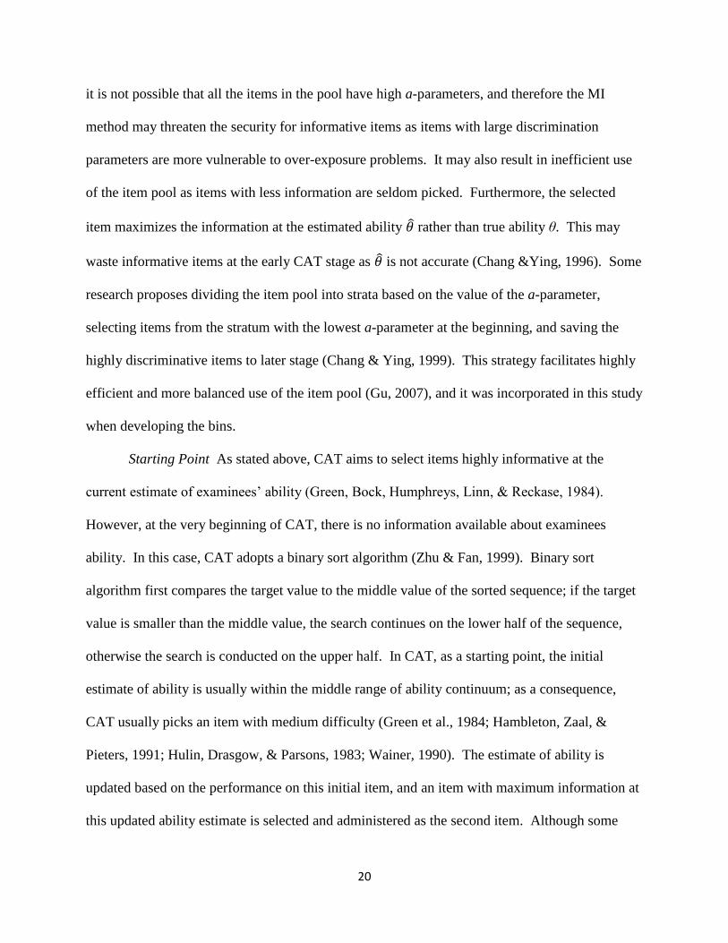
where is defined in function 2.3. Figure 2.6 shows the information for five polytomous
items with four score categories (see item parameters in Table 2.1). It indicates that items with
high discrimination parameter have more information, and the information function is more
peaked when the distance between the first and last threshold parameters is shorter (Dodd &
Koch, 1987). When the distance between two adjacent threshold parameters is large, the
information function may not be unimodal (Akkermans & Muraki, 1997; Muraki, 1993).
Furthermore, if the step parameters are in an ascending order, the information function will be
more peaked.
-4 -3 -2 -1 0 1 2 3 40
0.05
0.1
0.15
0.2
0.25
0.3
0.35
0.4
Ite
m Info
rmation
a=1 b=-0.5
a=1.2 b=-0.5
a=1.2 b=0.5
19
Table 2.1 Item Parameters for a GPCM Item
a b d0 d1 d2 d3
0.93 -1.28 0 1.3 1.07 -2.37
0.73 -1.28 0 1.3 1.07 2.37
0.93 -1.28 0 2 1.07 -3.07
0.93 -1.28 0 1.07 2 -3.07
0.93 -1.28 0 -2.37 1.07 1.3
Figure 2.6 Item Information for Polytomous Items with GPCM
The sum of item information across items is the test information, which is equal to the
reciprocal of variance of estimation, as indicated below:
( | ) =
=
∑
(2.8)
where is the maximum likelihood estimate (MLE) of true ability , and l is the likelihood of a
given response pattern. As larger information indicates smaller standard error, items with higher
information are always desired in CAT when adopting the MI item selection method. However
-4 -3 -2 -1 0 1 2 3 40
1
2
3
4
5
6
Ite
m Info
rmation
Item 1
Item 2
Item 3
Item 4
Item 5
20
it is not possible that all the items in the pool have high a-parameters, and therefore the MI
method may threaten the security for informative items as items with large discrimination
parameters are more vulnerable to over-exposure problems. It may also result in inefficient use
of the item pool as items with less information are seldom picked. Furthermore, the selected
item maximizes the information at the estimated ability rather than true ability θ. This may
waste informative items at the early CAT stage as is not accurate (Chang &Ying, 1996). Some
research proposes dividing the item pool into strata based on the value of the a-parameter,
selecting items from the stratum with the lowest a-parameter at the beginning, and saving the
highly discriminative items to later stage (Chang & Ying, 1999). This strategy facilitates highly
efficient and more balanced use of the item pool (Gu, 2007), and it was incorporated in this study
when developing the bins.
Starting Point As stated above, CAT aims to select items highly informative at the
current estimate of examinees’ ability (Green, Bock, Humphreys, Linn, & Reckase, 1984).
However, at the very beginning of CAT, there is no information available about examinees
ability. In this case, CAT adopts a binary sort algorithm (Zhu & Fan, 1999). Binary sort
algorithm first compares the target value to the middle value of the sorted sequence; if the target
value is smaller than the middle value, the search continues on the lower half of the sequence,
otherwise the search is conducted on the upper half. In CAT, as a starting point, the initial
estimate of ability is usually within the middle range of ability continuum; as a consequence,
CAT usually picks an item with medium difficulty (Green et al., 1984; Hambleton, Zaal, &
Pieters, 1991; Hulin, Drasgow, & Parsons, 1983; Wainer, 1990). The estimate of ability is
updated based on the performance on this initial item, and an item with maximum information at
this updated ability estimate is selected and administered as the second item. Although some
21
research claims that the starting point is unimportant as long as CAT has reasonable length, e.g.,
more than 25 items (Lord, 1987; Hulin et al., 1983), Wainer and Kiely (1987) argue that
inappropriate starting point may increase test anxiety and frustration. Moreover, too easy or too
hard items provide little information for estimating the examinee’s ability (Green et al., 1984).
Hence in this study the starting point was located around the medium ability level, as most CAT
practice and research do.
Scoring Rule In CAT, after administering each item, the examinee’s ability will be re-
estimated. The two approaches most widely used for updating ability estimate are: (1) maximum
likelihood estimation, including maximum likelihood estimate (MLE; Lord, 1980; Birnbaum,
1968), marginal maximum likelihood (MML; Bock & Aitkin, 1981), and weighed likelihood
estimation (WLE; Warm, 1989) and (2) Bayesian estimation, including expected a posteriori
(EAP; Bock & Aitkin, 1981) and maximum a posteriori (MAP; Samejima, 1969). As MLE is
the basis of all the methods in the first category and was applied in this study, it will be
introduced first; then a brief description of the Bayesian estimation is provided.
In MLE, for a given examinee, the responses across test items are assumed to be locally
independent, so the likelihood is the product of probabilities of getting a correct or incorrect
response on each item. In 2PLM or 3PLM, the likelihood is:
L(u|θ) = ∏ (2.9)
where u is the response string, pi ( is the probability of getting response ui (ui=0 for
incorrect response and 1 for correct response) on item i given an examinee’s with true ability θ
and item parameter , and n is the number of administered items. The maximum likelihood
estimate of an examinee’s true ability θ is the value that maximizes L given response pattern u
22
and the collection of item parameters . For GPCM, the response has more than two
plausible values and the likelihood can be formulized as:
L(u|θ) = ∏ (2.10)
where k is the score on item i, and other notations keep the same as Function 2.9.
MLE is also the value where the first derivative of L is equal to 0 (Pfanzagl, 1994), as:
(2.11)
As no closed-form expression is available for MLE of , it’s often calculated through an
iterative numerical procedure like the Newton-Raphson algorithm (Segall, 2005). MLE has
desirable property of asymptotic consistency, i.e., as sample size n goes up, MLE will converge
in probability to its true value. In addition, MLE is also asymptotically normal, i.e., has a
normal distribution with the mean equal to true value θ, and the variance identical to the
reciprocal of the test information (see Function 2.8). Due to these theoretical characteristics,
MLE is widely used in CAT (Samejima, 1969; Hambleton & Swaminathan, 1985). However,
when the response string consists of only correct or incorrect responses (or, only highest or
lowest score category in polytomous-item-based tests), a positive or negative infinite ability
estimate will result, which causes problems for item selection in next step. This can be solved by
setting an arbitrary boundary (e.g., -4 and +4) for estimates from such response patterns, or by
adopting a Bayesian estimate until the examinee has both correct and incorrect responses.
Another problem related to MLE is that it is biased. is over-estimated for positive θ and
underestimated for negative θ, and the magnitude of bias is larger at extreme θ values (Lord,
1980). This trend is obvious in short tests, while in long tests MLE is asymptotically unbiased.
An alternative procedure to MLE is a Bayesian method, which has an assumption of a
prior distribution of ability, i.e., the examinee comes from a population with a normal
23
distribution of ability where mean and variance are known. After answering each test question, a
posterior distribution is formed by combining the prior distribution with the response, as:
(2.12)
where is the posterior distribution, is the prior distribution, and is the
likelihood of a given response string u in the population, which is a constant. If the mean of this
posterior distribution is used to update the ability estimate, this approach is named as expected a
posteriori (EAP); if the mode is used, it’s named as maximum a posteriori (MAP). When
administering the same number of items, the Bayesian method yields smaller standard error than
MLE by absorbing additional information from prior distribution. And the Bayesian method can
always produce a finite estimate. However, though Bayesian method may overcome some
drawbacks of MLE, one limitation is that for the Bayesian method the selection of prior may
have significant influence on the final estimate, as the estimates will shrink to the mean of the
prior. The estimate can be seriously biased if an inappropriate prior is used (Wang & Vispoel,
1998; Lord, 1986; Warm, 1989).
There have been numerous studies comparing ability estimation methods in CAT, in both
dichotomous and polytomous cases (Chen, Hou, Fitzpatrick, & Dodd, 1997; Chen, Hou, & Dodd,
1998; Wang & Wang, 2001; Ho, 2010). Generally, the results suggest comparable effects of
MLE and other methods (Ho, 2010). In this study, MLE was used to yield ability estimates.
Stopping Rule Two strategies are widely used to determine when to terminate a CAT
process: fixed length and variable length. When adopting fixed-length rule, all examinees are
required to take the same number of items. For example, all the examinees take a 30-item test.
In fixed-length tests, different examinees spend similar testing time, which facilitates the test
administration, and standardizes the testing conditions and related testing-fatigue (Gu, 2007).
24
One disadvantage of fixed-length test is that the measurement precision varies among examinees,
which causes problems for calculation and reporting reliability across ability levels (Segall, 2005;
Gu, 2007). The other method, variable-length rule, pre-specifies a level of precision based on
ML information or Bayesian posterior variance statistics, and continually administers items until
the estimate of ability reaches this target precision. Compared with fixed-length test, variable-
length rule may improve test efficiency and item pool use, as it often minimizes test length while
remaining high test accuracy (Bergstrom & Lunz, 1999). The drawback of this procedure is that
it’s difficult to explain to the examinees why they have to take test of different length.
Furthermore, in variable-length test, examinees of extremely high or low proficiency are likely to
receive long tests, especially when the item pool has no highly informative items for these
extreme examinees, and then different fatigue level may have an effect on the results from the
CAT (Segall, Moreno, & Hetter, 1997). Segall (2005) suggests imposing some adjustments to
moderate some of the operational difficulties, such as implementing an upper-bound for the
variable-length tests.
All of these components discussed above influence the design and the effectiveness of the
CAT procedure (Chang, Qian, & Ying, 2001; Kingsbury & Zara, 1989; Zhou, 2011). In addition,
some practical issues regarding test security, validity, security and examinees’ psychological
experience, should also be taken into consideration when designing a CAT. For example, in
CAT item selection, some items are used in most of the administrations, while other items are
seldom used; how frequently an item appears in a test (i.e., the item exposure rate) depends on its
psychometric properties, overall examinee ability distribution in the test-taking population, and
the quality and availability of other items in the pool (Gu, 2007). Items with high exposure rates
may cause security problems and impact the test’s validity, and items that are rarely used
25
indicate a waste of resources spent on item developing. Several exposure control methods have
been developed to avoid the over-exposure and maintain reasonable item usage (Cheng & Chang,
2009; Hetter & Sympson, 1997). Another requirement for CAT is to guarantee each test meets
the same test specifications and covers all the desired contents (i.e., keep the content balanced).
The requirements for obtaining higher information, maintaining exposure rate and keeping the
content balanced have direct influence on the test assembly, which will be further discussed in
next section.
2.3 CAT Assembly Approaches
2.3.1 Goals of CAT Assembly
Generally there are three requirements for assembling a CAT (Davey, 2005). First, as
stated earlier, one of the major targets for CAT is to achieve higher measurement efficiency by
administering informative items. By matching item difficulty to the current examinee’s ability
estimate, CAT can reduce test length without losing measurement precision (Lord, 1980; Weiss,
1983; Robin, 2005). The strategies of selecting highly informative items have been stated in
detail in the previous section. The second hurdle in CAT development is to balance content. In
conventional paper-pencil testing, all the examinees take the same test, and the requirement for
content coverage can be met easily as long as the single test form fulfills the test specification.
In contrast, CAT builds individualized tests by adaptively selecting items, and different tests
should have comparable content coverage specified by the test blueprint. As a consequence, the
item selection method should be adjusted to achieve maximized information while ensuring
content balance (Cordova, 1997; Stocking & Swanson, 1993; van der Linden, 1998; van der
Linden & Reese, 1998; van der Linden, 2005). Considering the threats to test validity and
fairness brought by an unbalanced test, several models such as the weighted penalty model
26
(WPM) and the weighted deviation algorithm (WDA) have been developed to ensure content
balance. The third requirement is to avoid item over-exposure and ensure test security. Item
exposure rate is the ratio between the number of times a certain item is administered and the total
number of examinees. Extremely low exposure rate means the item is rarely used and indicates a
waste, while high exposure rate threatens test security and validity. The problem is more severe
when the item development is time consuming and expensive (e.g., for polytomous items and
set-based items) and when the test is high-stakes. As shown earlier, selecting items merely
according to a statistical criterion (e.g., maximum information) is the main reason for item over-
exposure (van der Linden, 2004). Several procedures, such as randomization, conditional
selection procedure, and a-stratified strategy have been applied to control exposure rate.
In summary, the objective of CAT assembly is to construct efficient tests, and meet all
the demands for content balance and test security (He, 2010; Davey & Parshall, 1995; Wainer,
Dorans, Flaugher, Green, Mislevy, Steinberg, & Thissen, 1990; Sands, Waters, & McBride, 1997;
van der Linden, & Glas, 2000; Mills, Potenza, Fremer, & Ward, 2002). Actually when a CAT
moves to operational implementation, besides these three main requirements, sometimes some
other issues have to be taken into account. For example, some tests, like NCLEX, have limits on
total testing time. Other issues include how to eliminate the item context effect in CAT as the
existing location of an item may influence the examinee’s performance on the same question,
how to diminish the examinee nervousness at the beginning of the test, etc. Some of these issues
will be addressed in this study. These requirements are always in conflict with one another and a
compromise to balance all goals is needed in test assembly (Davey, 2005).
27
2.3.2 Assembly Design in CAT
A variety of test assembly methods have been proposed and successfully implemented,
including the constrained CAT method (CCAT; Kingsbury & Zara, 1991), the modified CCAT
(MCCAT; Leung, Chang, & Hau, 2003), the weighted deviations model (WDM; Stocking &
Swanson, 1993), the modified multinomial model (MMM; Chen & Ankenmann, 2004), the
weighted penalty model (WPM; Shin, Chien, Way, & Swanson, 2009), the maximum priority
index (MPI) method (Cheng & Chang, 2009), the shadow-test approach (STA; van der Linden &
Reese, 1998), and bin-structured method (Davey, 2005). Many of studies have compared these
methods (Chen & Ankenmann, 2004; Cheng & Chang; 2009; van der Linden, 2005). Among
these methods, CCAT, MCCAT, MMM and bin-structured method partition the item pool into
several sub-pools by some key features, such as content area, and the items are drawn from these
sub-pools in a sequential way. One limitation of these methods is that they are applicable when
an item only carries limited attribute, i.e., the ones used to divide the item pool (He, 2010). In
contrast, the STA, the WDM, the WPM, and the MPI can handle more constraints and are more
flexible. Among these four methods, the STA adopts a mathematical programming method
while the others are heuristic. This study involves one method from each of these two categories
of test assembly approaches: STA and bin-structured approach. The reason for choosing the
STA is that it can deal with complex constraints and does not require judgment-based weights,
which are not available for test to be used in this study. On the other hand, though the bin-
structured method holds advantages over conventional methods especially in terms of exposure
control and standardizing the look of the test, and is promising for future utilization, it hasn’t
been studied thoroughly, and no research is conducted in mixed-item-format case. This study
aims to fill in this void. A more detailed description of these two methods is provided below.
28
STA The STA was proposed by van der Linden and Reese (1998) and since then has
been widely researched in different CAT contexts (He, 2010). In general, the STA belongs to
the constrained combination optimization problem (Nemhauser & Wolsey, 1988; Rao, 1985;
Wagner, 1969), where the goal is to find a solution optimal in terms of one attribute while
meeting a variety of constraints with respect to other attributes. As a consequence, two kinds of
test specifications are defined and distinguished in STA: (1) objective, which requires a test
attribute function (e.g., test information or posterior variance of estimate) to reach the maximum
or minimum value, and can be written as a function to be optimized; and (2) constraint, which
limits an attribute (e.g., number of items in each content area) within a certain range, and can be
formulated as equations (or inequalities). The constraints can be further classified into three
categories: constraints on categorical attributes (e.g., item format), on quantitative properties
(e.g., expected testing time), and on item dependencies (e.g., item enemy). Then the test
assembly issue is an optimal problem with a set of the constraints. In other words, in STA the
test information at the current ability estimate can be regarded as the objective function to be
optimized, and this optimization problem is subject to all other specifications, which are viewed
as constraints (van der Linden, 1998; van der Linden, Ariel, & Veldkamp, 2006; Veldkamp &
van der Linden, 2000). Here is an example for how STA defines the goal of test assembly as a
constrained combination optimization problem.
Objective: maximize ∑ ( ) , i.e., maximize test information at , where N is the
item number in the whole item pool and xi is an indicator variable specifying which items are
included in the test.
Constraints: , i=1,2,…N. i.e., if item i is selected when assembling a shadow test,
is valued as 1; otherwise is 0;
29
∑ , i.e., less than 5 items of Format 1 (e.g., dichotomous items);
∑ , i.e., more than 8 items of Format 2 (e.g., polytomous items);
∑ , i.e., less than 10 items in Content Area 1;
∑ , i.e., 3 items in Content Area 2;
∑ , i.e., more than 9 items in Content Area 3;
∑ , i.e., the total test length is 20 items;
+ ≤ 1, i.e., Item 33 and Item 54 are exclusive;
∑ , i.e., the total word count is less than 2000, where wi is the
number of words in item i.
The basic idea of STA is to assemble an optimal test using linear programming. In STA,
a full-length test satisfying all requirements and with maximum information is assembled before
selecting an item to be administered, and is named a shadow test, as shown in the example above;
then the item with maximum information is picked from this shadow test instead of from the
pool. In other words, the item administered is the one in the current shadow test that is optimal
at the current ability estimate and has not already been used. After administering the new item,
the shadow test is released to the pool and the ability is re-estimated. This creation of a shadow
test and selecting an item to be administered is repeated until the stopping rule is met. He (2010)
provides a brief description of a typical STA procedure:
Step 1: Give an initial estimate of the ability as the starting point.
Step 2: Assemble the first shadow test that satisfies all requirements (e.g., constraints for
content area, item format, total testing time, exposure rate, etc.) and optimizes the objective
function (e.g., maximize the test information).
30
Step 3: From the shadow test assembled in Step 2, select and administer the item that can
provide maximum information at the current ability estimate, and return all the other items in the
shadow test into the bank.
Step 4: Update the ability estimate according to some scoring rule (e.g., MLE).
Step 5: Assemble a new shadow test which is optimal and meets all constraints while
containing items already administered.
Step 6: Repeat Steps 2-5 until a stopping rule (e.g., a pre-specified test length) is reached.
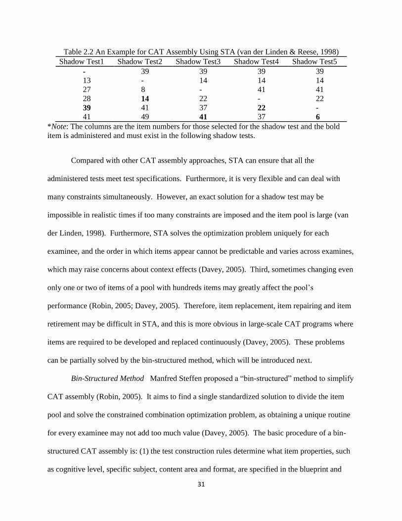
This description indicates several properties of a shadow test: (1) it’s a full-size linear test
as no sequential selection is performed within a given shadow test; (2) it includes all items
already taken by the examinee; (3) it provides maximum information at the current ability
estimate; and (4) it satisfies all the test specifications required by the CAT. An example by van
der Linden and Reese (1998) may be helpful to understand the procedure: assume the goal is to
assemble a 5-item CAT for a given examinee. In Table 2.2, each column indicates a shadow test
assembled at the current , the bold numbers are the item with maximum information selected to
be administered, and all the non-bold items will be released into the pool. The items in the upper
triangle have been administered to him/her. It can be seen that the bold numbers enter into the
next column of the upper triangle, as the items which are administered must be in the new
assembled shadow-test. For this examinee, Item 39, 14, 41, 22, and 6 are administered.
31
Table 2.2 An Example for CAT Assembly Using STA (van der Linden & Reese, 1998)
Shadow Test1 Shadow Test2 Shadow Test3 Shadow Test4 Shadow Test5
- 39 39 39 39
13 - 14 14 14
27 8 - 41 41
28 14 22 - 22
39 41 37 22 -
41 49 41 37 6
*Note: The columns are the item numbers for those selected for the shadow test and the bold
item is administered and must exist in the following shadow tests.
Compared with other CAT assembly approaches, STA can ensure that all the
administered tests meet test specifications. Furthermore, it is very flexible and can deal with
many constraints simultaneously. However, an exact solution for a shadow test may be
impossible in realistic times if too many constraints are imposed and the item pool is large (van
der Linden, 1998). Furthermore, STA solves the optimization problem uniquely for each
examinee, and the order in which items appear cannot be predictable and varies across examines,
which may raise concerns about context effects (Davey, 2005). Third, sometimes changing even
only one or two of items of a pool with hundreds items may greatly affect the pool’s
performance (Robin, 2005; Davey, 2005). Therefore, item replacement, item repairing and item
retirement may be difficult in STA, and this is more obvious in large-scale CAT programs where
items are required to be developed and replaced continuously (Davey, 2005). These problems
can be partially solved by the bin-structured method, which will be introduced next.
Bin-Structured Method Manfred Steffen proposed a “bin-structured” method to simplify
CAT assembly (Robin, 2005). It aims to find a single standardized solution to divide the item
pool and solve the constrained combination optimization problem, as obtaining a unique routine
for every examinee may not add too much value (Davey, 2005). The basic procedure of a bin-
structured CAT assembly is: (1) the test construction rules determine what item properties, such
as cognitive level, specific subject, content area and format, are specified in the blueprint and
32
will guide the CAT assembly; (2) the item pool is divided into non-overlapping and
homogeneous clusters according to these identified item properties, and each cluster is regarded
as a bin; the items in the same bin are interchangeable in terms of these test construction rules,
and the number of bins is equal to the desired test length; and (3) then test developers determine
a sequence to arrange these bins. Such an ordered sequence is called a template and is applied to
all examinees. It satisfies all the test specification so it’s impossible to violate the constraints.
During item administration, each item is selected from one bin, rather than from all the available
items in the pool. Each bin only contributes one item. As the test constraints relevant to test
construction properties such as content area have been handled in the design of the template, the
main target for item selection in each step is to select an informative item while controlling
exposure rate in each bin. Therefore, the specific solution for any examinee is unique and
adaptive, while the assembled test is more standardized compared with STA.
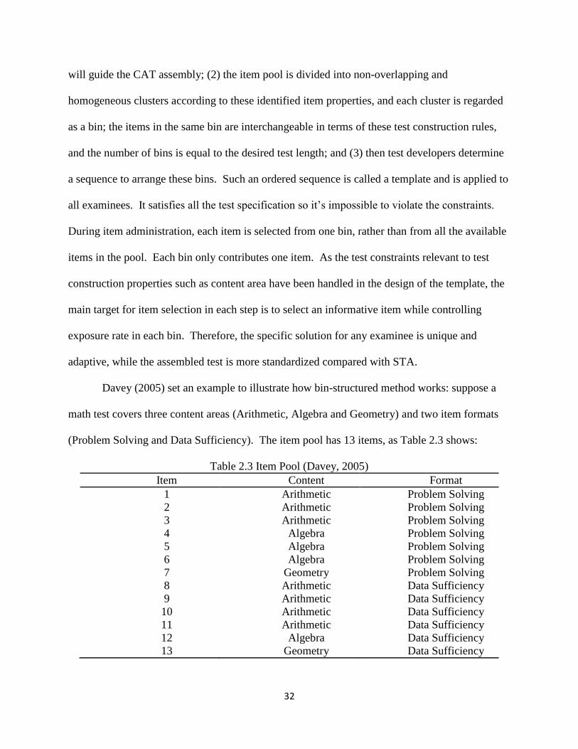
Davey (2005) set an example to illustrate how bin-structured method works: suppose a
math test covers three content areas (Arithmetic, Algebra and Geometry) and two item formats
(Problem Solving and Data Sufficiency). The item pool has 13 items, as Table 2.3 shows:
Table 2.3 Item Pool (Davey, 2005)
Item Content Format
1 Arithmetic Problem Solving
2 Arithmetic Problem Solving
3 Arithmetic Problem Solving
4 Algebra Problem Solving
5 Algebra Problem Solving
6 Algebra Problem Solving
7 Geometry Problem Solving
8 Arithmetic Data Sufficiency
9 Arithmetic Data Sufficiency
10 Arithmetic Data Sufficiency
11 Arithmetic Data Sufficiency
12 Algebra Data Sufficiency
13 Geometry Data Sufficiency
33
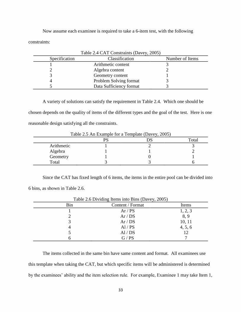
Now assume each examinee is required to take a 6-item test, with the following
constraints:
Table 2.4 CAT Constraints (Davey, 2005)
Specification Classification Number of Items
1 Arithmetic content 3
2 Algebra content 2
3 Geometry content 1
4 Problem Solving format 3
5 Data Sufficiency format 3
A variety of solutions can satisfy the requirement in Table 2.4. Which one should be
chosen depends on the quality of items of the different types and the goal of the test. Here is one
reasonable design satisfying all the constraints.
Table 2.5 An Example for a Template (Davey, 2005)
PS DS Total
Arithmetic 1 2 3
Algebra 1 1 2
Geometry 1 0 1
Total 3 3 6
Since the CAT has fixed length of 6 items, the items in the entire pool can be divided into
6 bins, as shown in Table 2.6.
Table 2.6 Dividing Items into Bins (Davey, 2005)
Bin Content / Format Items
1 Ar / PS 1, 2, 3
2 Ar / DS 8, 9
3 Ar / DS 10, 11
4 Al / PS 4, 5, 6
5 Al / DS 12
6 G / PS 7
The items collected in the same bin have same content and format. All examinees use
this template when taking the CAT, but which specific items will be administered is determined
by the examinees’ ability and the item selection rule. For example, Examinee 1 may take Item 1,
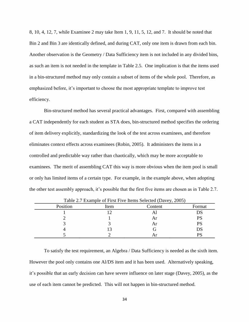
34
8, 10, 4, 12, 7, while Examinee 2 may take Item 1, 9, 11, 5, 12, and 7. It should be noted that
Bin 2 and Bin 3 are identically defined, and during CAT, only one item is drawn from each bin.
Another observation is the Geometry / Data Sufficiency item is not included in any divided bins,
as such an item is not needed in the template in Table 2.5. One implication is that the items used
in a bin-structured method may only contain a subset of items of the whole pool. Therefore, as
emphasized before, it’s important to choose the most appropriate template to improve test
efficiency.
Bin-structured method has several practical advantages. First, compared with assembling
a CAT independently for each student as STA does, bin-structured method specifies the ordering
of item delivery explicitly, standardizing the look of the test across examinees, and therefore
eliminates context effects across examinees (Robin, 2005). It administers the items in a
controlled and predictable way rather than chaotically, which may be more acceptable to
examinees. The merit of assembling CAT this way is more obvious when the item pool is small
or only has limited items of a certain type. For example, in the example above, when adopting
the other test assembly approach, it’s possible that the first five items are chosen as in Table 2.7.
Table 2.7 Example of First Five Items Selected (Davey, 2005)
Position Item Content Format
1 12 Al DS
2 1 Ar PS
3 3 Ar PS
4 13 G DS
5 2 Ar PS
To satisfy the test requirement, an Algebra / Data Sufficiency is needed as the sixth item.
However the pool only contains one Al/DS item and it has been used. Alternatively speaking,
it’s possible that an early decision can have severe influence on later stage (Davey, 2005), as the
use of each item cannot be predicted. This will not happen in bin-structured method.
35
Because in bin-structured method the bins do not interact with each other, exposure
control can be conducted within bins without influencing the other bins or the entire pool, and
item replacement is more convenient (Davey, 2005). Other CAT assembly methods such as
WDA often require tedious preliminary simulations to control item exposure (Robin, 2005).
Furthermore, it guarantees that test construction rules are satisfied by developing appropriate
template in advance, which significantly simplifies item selection and test administration. Also,
as for each step the item selection is restricted in one bin, an item only competes with items in
the same bin and therefore the calculation burden is greatly reduced. Finally, the control for item
enemies is easy: the item enemies can be put in one bin; choosing one will exclude its enemies
because each bin only contributes one item.
Although bin-structured approach adopts a uniform routine for all the examinees and
seems less flexible, it’s no less adaptive if the bins can be developed properly (Davey, 2005).
Furthermore, it can be combined with other test assembly methods. Robin (2005) incorporates
bin-structured model into WDA, and finds the bin-structured approach works equally well
compared with conventional WDA in terms of measurement efficiency, content balance,
exposure rate, and efficient item use. However, as a relatively new method, research on the bin-
structured method is still rare, and none uses mixed-item-format based CAT. And no study
investigates what factor may influence the effect of bin-structured method.

36
Chapter 3: Methods and Procedures
The main purposes of this study were (1) to investigate whether the mixed-item-based
CAT had advantages over the dichotomous-item-based CAT and what challenges it brought; and
(2) to compare the STA with the bin-structured method in mixed-item CAT assembly, and to
explore what were some factors that might influence any assembly effect. A simulation study
was conducted, as a simulation can set a variety of conditions to evaluate the effects of different
factors, and also provide the true value as a baseline to assess bias. This chapter describes the
methodological framework of the simulation study. The first section describes the procedure of
developing the item pools. Next, the procedure for CAT simulation is described. Specifically,
the CAT specifications with respect to content area, item format and required cognitive skills are
described. This section also illustrates how the STA and bin-structured methods assemble the
CAT with different constraint sets. The final section describes the criteria that are used to assess
the CAT assembly approaches.
3.1 Generate Item Pools
3.1.1 Data Source
The item pool was based on the Education Quality and Accountability Office (EQAO)
Grade 10 Ontario Secondary School Literacy Test (OSSLT; http://www.eqao.com/). EQAO has
been existed for almost 20 years with the purpose of providing comparable year-to-year
information on student learning. EQAO provides several province-wide assessments: the
Assessments of Reading, Writing and Mathematics, Primary and Junior Divisions; the Grade 9
Assessment of Mathematics; and the OSSLT. To simulate the situation where both
dichotomously and polytomously scored items (including polytomous items and testlets) were
involved, this study was focused on the OSSLT. The OSSLT is administered on an annual basis
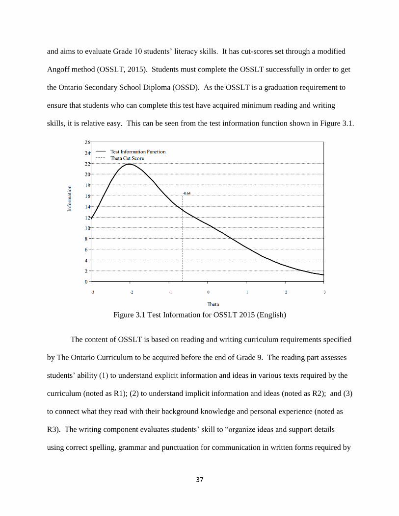
37
and aims to evaluate Grade 10 students’ literacy skills. It has cut-scores set through a modified
Angoff method (OSSLT, 2015). Students must complete the OSSLT successfully in order to get
the Ontario Secondary School Diploma (OSSD). As the OSSLT is a graduation requirement to
ensure that students who can complete this test have acquired minimum reading and writing
skills, it is relative easy. This can be seen from the test information function shown in Figure 3.1.
Figure 3.1 Test Information for OSSLT 2015 (English)
The content of OSSLT is based on reading and writing curriculum requirements specified
by The Ontario Curriculum to be acquired before the end of Grade 9. The reading part assesses
students’ ability (1) to understand explicit information and ideas in various texts required by the
curriculum (noted as R1); (2) to understand implicit information and ideas (noted as R2); and (3)
to connect what they read with their background knowledge and personal experience (noted as
R3). The writing component evaluates students’ skill to “organize ideas and support details
using correct spelling, grammar and punctuation for communication in written forms required by

38
the curriculum” (OSSLT, 2015). Specifically, four cognitive skills are measured by the writing
test: (1) to organize main ideas (noted as W1); (2) to organize relevant information (noted as
W2); (3) to use conventions (noted as W3); and (4) to develop a topic (noted as W4).
The data in this study is from the performance of English-speaking student on the 2015
Operational Test of OSSLT. The 2015 OSSLT contains 38 multiple-choice, 4 open-response
questions, 4 short writing and 4 long writing questions. But the long writing items were not used
in this study as they were not field-tested, and real CAT seldom adopts such an item format.
That left 8 polytomous-scoring items consists of six 4-point Likert scale items and two 3-point
Likert scale items, but the 3-point Likert scale scores were excluded from this study as they
didn’t perform well in previous OSSLT analyses. Hence, the entire study was based on 44 items,
among which 34 are reading items and 10 are writing items (see Table 3.1).
Table 3.1 OSSLT Test Specification
Reading Writing Total
R1 R2 R3 W1 W2 W3 W4
Dichotomous 7 17 6 2 2 4 0 38
Polytomous 0 2 2 0 0 0 2 6
Test forms are assembled for both English and French versions from March 2014 field-
test materials. Before administrating the test, all materials and questions are reviewed and
approved by a content review committee (i.e., Assessment Development Committee) which
consists of educators from across the province. Meanwhile, another group of equity experts,
known as the Sensitivity Committee, review all test items and materials to guarantee they are fair
and free from bias. In the field test, approximately 5000 English students and 500 French
students are randomly selected and answer each multiple-choice item. The sample used to score
the polytomous items (including open-response items and short writing items) contain1200
students in English and 500 students in French. EQAO requires comparable procedures for both

39
English and French students, but the French sample size is small. Therefore when calibrating the
items with 3PLM, OSSLT fix the a-parameter of dichotomous items at 0.588 and the c-
parameter at 0.2. This modified 3PLM is also known a modified Rasch model. The slope of the
GPCM model is also fixed at 0.588. The IRT parameters, classical test theory (CTT) difficulty,
and cognitive skills measured are available in OSSLT report (OSSLT, 2014). Overall, OSSLT
can provide reliable, objective and high-quality scores (OSSLT, 2005). The reliability
coefficient is above 0.85, and the correct classification rate is 0.90 (OSSLT, 2014).
3.1.2 Generate the Original Item Pool
As stated before, 44 items were kept as the basis for this study, among which 38 were
dichotomous, and 6 (including polytomous items and testlets) adopted polytomous scoring with
four score categories. The item cloning method (Glas & van der Linden, 2003) was used to
expand the item pool size. The procedure for cloning items was: represent the parent item (i.e.,
the items which were used to produce the new items) as p = 1,..., P with item parameter , and
items within family p as ip = 1, ..., Ip. For each item, the item parameter is a vector noted as .
For instance, in 3PLM, ]. was assumed to have a multivariate normal
distribution:
~ N ( )
where is the mean of item parameters in family p, and is the covariance matrix. In this
study, for the GPCM, overall difficulty and thresholds were generated since the slopes were
fixed. was the vector consisting of average overall difficulty and thresholds of the 6
polytomous items in the original OSSLT tests, was the covariance matrix. All the 6 parent
item parameter values were drawn from the multivariate normal distribution with a mean of
and covariance of . Then, given the parent parameter , item parameters cloned within
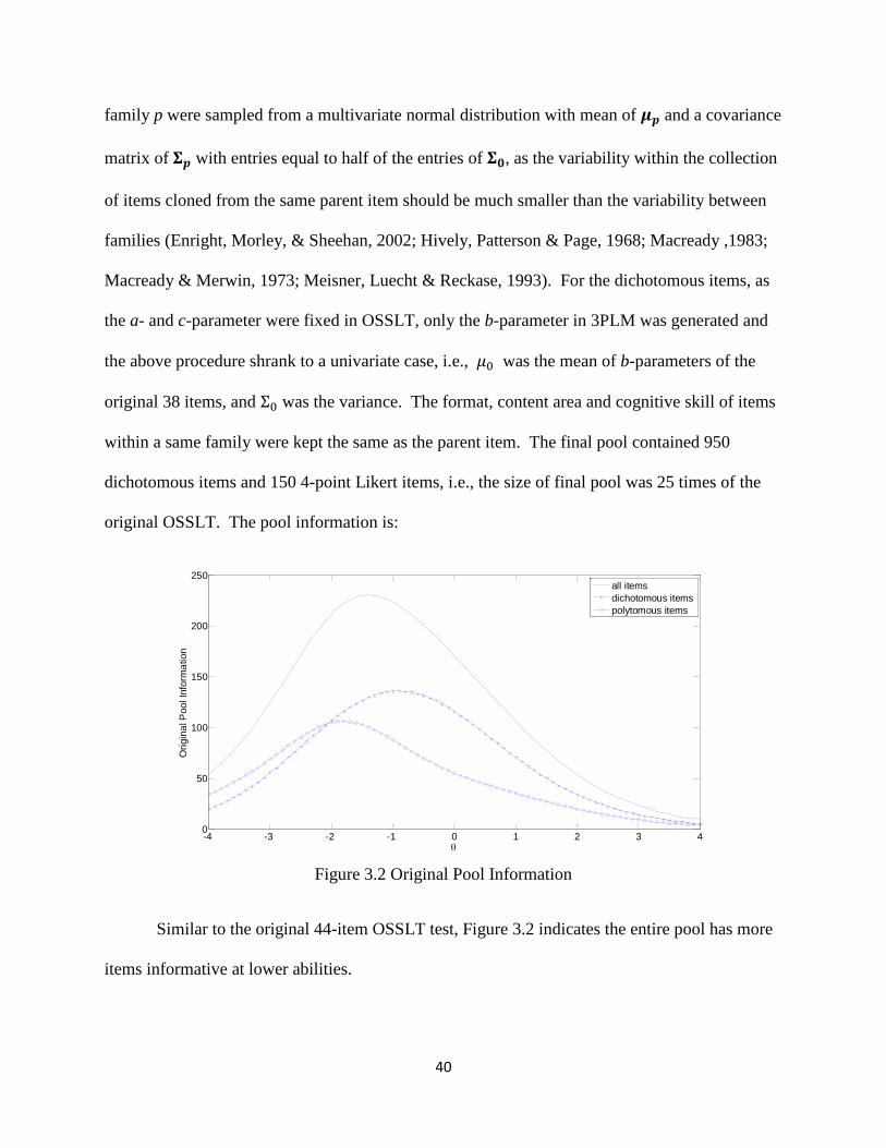
40
family p were sampled from a multivariate normal distribution with mean of and a covariance
matrix of with entries equal to half of the entries of , as the variability within the collection
of items cloned from the same parent item should be much smaller than the variability between
families (Enright, Morley, & Sheehan, 2002; Hively, Patterson & Page, 1968; Macready ,1983;
Macready & Merwin, 1973; Meisner, Luecht & Reckase, 1993). For the dichotomous items, as
the a- and c-parameter were fixed in OSSLT, only the b-parameter in 3PLM was generated and
the above procedure shrank to a univariate case, i.e., was the mean of b-parameters of the
original 38 items, and was the variance. The format, content area and cognitive skill of items
within a same family were kept the same as the parent item. The final pool contained 950
dichotomous items and 150 4-point Likert items, i.e., the size of final pool was 25 times of the
original OSSLT. The pool information is:
Figure 3.2 Original Pool Information
Similar to the original 44-item OSSLT test, Figure 3.2 indicates the entire pool has more
items informative at lower abilities.
-4 -3 -2 -1 0 1 2 3 40
50
100
150
200
250
Ori
gin
al P
ool In
form
ation
all items
dichotomous items
polytomous items
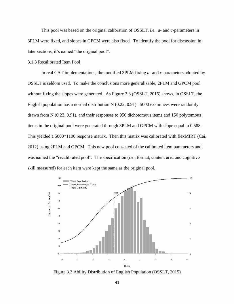
41
This pool was based on the original calibration of OSSLT, i.e., a- and c-parameters in
3PLM were fixed, and slopes in GPCM were also fixed. To identify the pool for discussion in
later sections, it’s named “the original pool”.
3.1.3 Recalibrated Item Pool
In real CAT implementations, the modified 3PLM fixing a- and c-parameters adopted by
OSSLT is seldom used. To make the conclusions more generalizable, 2PLM and GPCM pool
without fixing the slopes were generated. As Figure 3.3 (OSSLT, 2015) shows, in OSSLT, the
English population has a normal distribution N (0.22, 0.91). 5000 examinees were randomly
drawn from N (0.22, 0.91), and their responses to 950 dichotomous items and 150 polytomous
items in the original pool were generated through 3PLM and GPCM with slope equal to 0.588.
This yielded a 5000*1100 response matrix. Then this matrix was calibrated with flexMIRT (Cai,
2012) using 2PLM and GPCM. This new pool consisted of the calibrated item parameters and
was named the “recalibrated pool”. The specification (i.e., format, content area and cognitive
skill measured) for each item were kept the same as the original pool.
Figure 3.3 Ability Distribution of English Population (OSSLT, 2015)
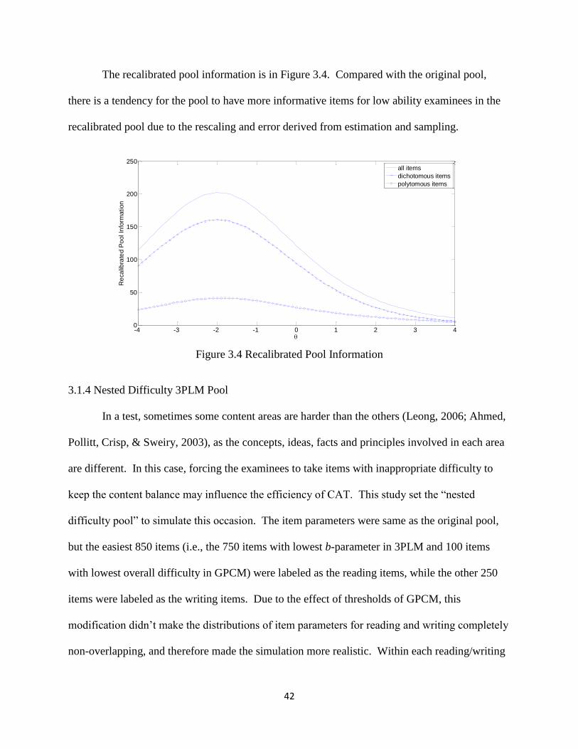
42
The recalibrated pool information is in Figure 3.4. Compared with the original pool,
there is a tendency for the pool to have more informative items for low ability examinees in the
recalibrated pool due to the rescaling and error derived from estimation and sampling.
Figure 3.4 Recalibrated Pool Information
3.1.4 Nested Difficulty 3PLM Pool
In a test, sometimes some content areas are harder than the others (Leong, 2006; Ahmed,
Pollitt, Crisp, & Sweiry, 2003), as the concepts, ideas, facts and principles involved in each area
are different. In this case, forcing the examinees to take items with inappropriate difficulty to
keep the content balance may influence the efficiency of CAT. This study set the “nested
difficulty pool” to simulate this occasion. The item parameters were same as the original pool,
but the easiest 850 items (i.e., the 750 items with lowest b-parameter in 3PLM and 100 items
with lowest overall difficulty in GPCM) were labeled as the reading items, while the other 250
items were labeled as the writing items. Due to the effect of thresholds of GPCM, this
modification didn’t make the distributions of item parameters for reading and writing completely
non-overlapping, and therefore made the simulation more realistic. Within each reading/writing
-4 -3 -2 -1 0 1 2 3 40
50
100
150
200
250
Re
ca
libra
ted P
ool In
form
ation
all items
dichotomous items
polytomous items
43
category, the cognitive skill requirement was randomly assigned to each item, while the
proportion of each skill category remained the same as the original item pool (i.e., the
distribution of items measuring each skill was the same as Table 3.1).
3.1.5 Nested Difficulty 2PLM Pool
The item parameters were the same as the recalibrated pool, but 750 items with lowest b-
parameters in 2PLM and 100 items with lowest overall difficulty in GPCM were regarded as the
writing items, and the other 250 items were writing items.
3.1.6 Balanced Item Pool
As both the original and recalibrated pool provided more information for the low-
proficiency students, a more balanced pool was generated to explore the influence of shape of
item pool on CAT assembly. For the dichotomous items, the a-parameters in 2PLM from the
recalibrated pool were retained, while b-parameters were simulated from a uniform distribution
within [-3, 3]. For the GPCM, the slopes and threshold parameters from recalibrated items were
retained, while the overall difficulty parameters were also randomly picked from [-3, 3]. The
specifications for each item, including the requirements for cognitive skills and content area,
were same as the recalibrated pool. Figure 3.5 shows that the information for the balanced item
pool is not skewed.
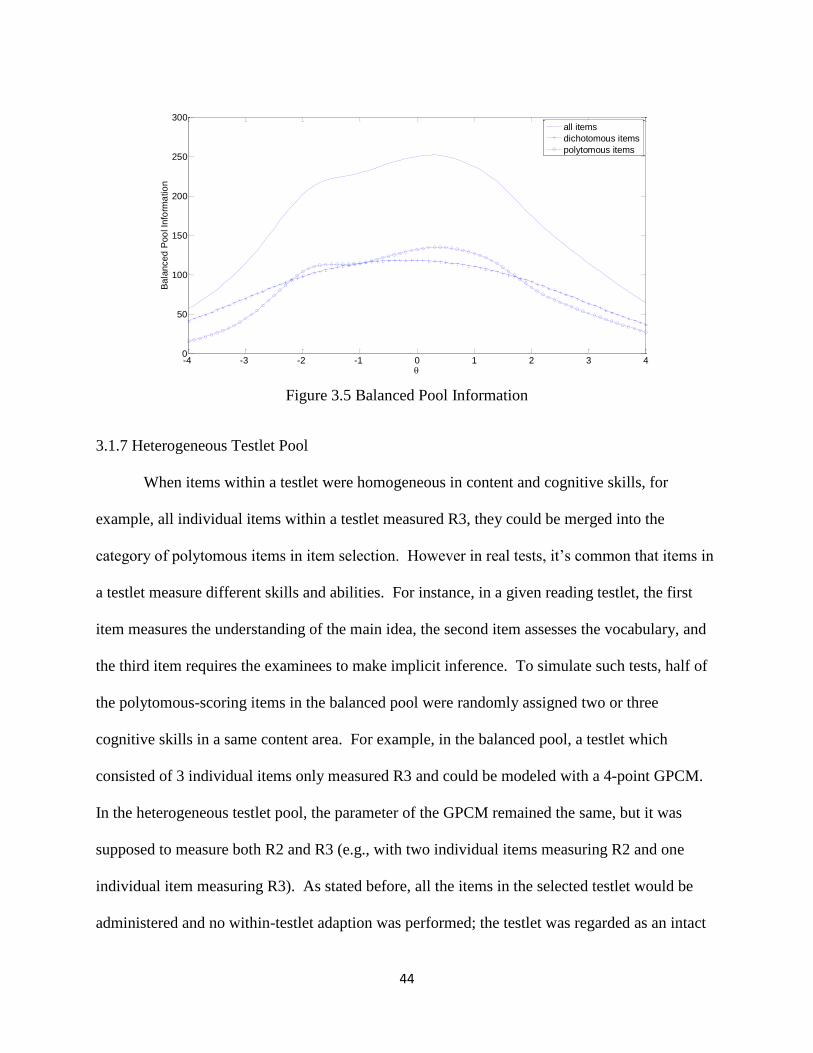
44
Figure 3.5 Balanced Pool Information
3.1.7 Heterogeneous Testlet Pool
When items within a testlet were homogeneous in content and cognitive skills, for
example, all individual items within a testlet measured R3, they could be merged into the
category of polytomous items in item selection. However in real tests, it’s common that items in
a testlet measure different skills and abilities. For instance, in a given reading testlet, the first
item measures the understanding of the main idea, the second item assesses the vocabulary, and
the third item requires the examinees to make implicit inference. To simulate such tests, half of
the polytomous-scoring items in the balanced pool were randomly assigned two or three
cognitive skills in a same content area. For example, in the balanced pool, a testlet which
consisted of 3 individual items only measured R3 and could be modeled with a 4-point GPCM.
In the heterogeneous testlet pool, the parameter of the GPCM remained the same, but it was
supposed to measure both R2 and R3 (e.g., with two individual items measuring R2 and one
individual item measuring R3). As stated before, all the items in the selected testlet would be
administered and no within-testlet adaption was performed; the testlet was regarded as an intact
-4 -3 -2 -1 0 1 2 3 40
50
100
150
200
250
300
Ba
lanced
Poo
l In
form
atio
n
all items
dichotomous items
polytomous items
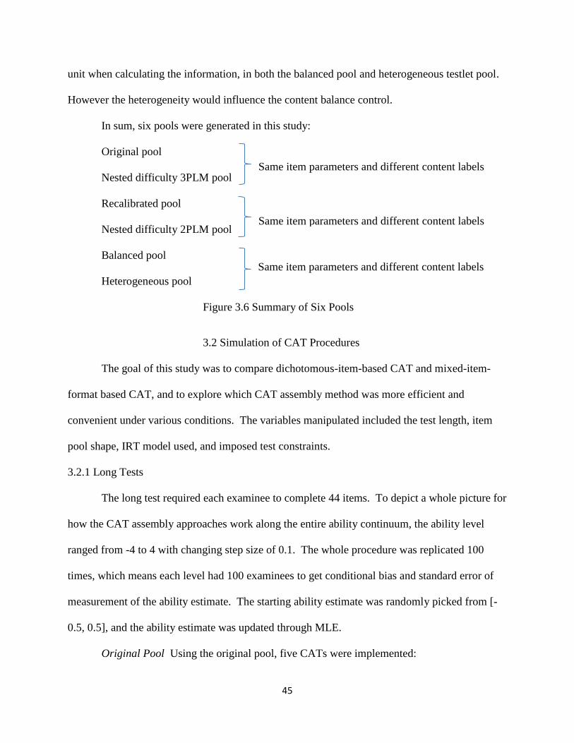
45
unit when calculating the information, in both the balanced pool and heterogeneous testlet pool.
However the heterogeneity would influence the content balance control.
In sum, six pools were generated in this study:
Original pool
Nested difficulty 3PLM pool
Recalibrated pool
Nested difficulty 2PLM pool
Balanced pool
Heterogeneous pool
Figure 3.6 Summary of Six Pools
3.2 Simulation of CAT Procedures
The goal of this study was to compare dichotomous-item-based CAT and mixed-item-
format based CAT, and to explore which CAT assembly method was more efficient and
convenient under various conditions. The variables manipulated included the test length, item
pool shape, IRT model used, and imposed test constraints.
3.2.1 Long Tests
The long test required each examinee to complete 44 items. To depict a whole picture for
how the CAT assembly approaches work along the entire ability continuum, the ability level
ranged from -4 to 4 with changing step size of 0.1. The whole procedure was replicated 100
times, which means each level had 100 examinees to get conditional bias and standard error of
measurement of the ability estimate. The starting ability estimate was randomly picked from [-
0.5, 0.5], and the ability estimate was updated through MLE.
Original Pool Using the original pool, five CATs were implemented:
Same item parameters and different content labels
Same item parameters and different content labels
Same item parameters and different content labels
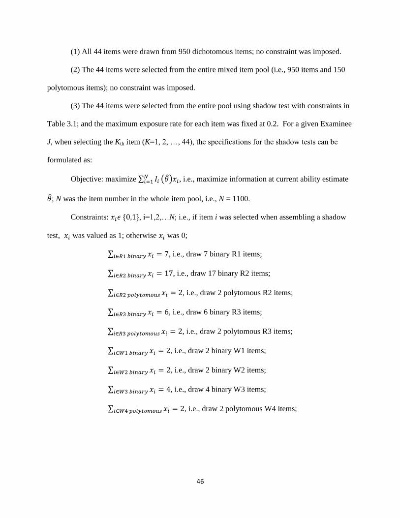
46
(1) All 44 items were drawn from 950 dichotomous items; no constraint was imposed.
(2) The 44 items were selected from the entire mixed item pool (i.e., 950 items and 150
polytomous items); no constraint was imposed.
(3) The 44 items were selected from the entire pool using shadow test with constraints in
Table 3.1; and the maximum exposure rate for each item was fixed at 0.2. For a given Examinee
J, when selecting the Kth item (K=1, 2, …, 44), the specifications for the shadow tests can be
formulated as:
Objective: maximize ∑ ( ) , i.e., maximize information at current ability estimate
; N was the item number in the whole item pool, i.e., N = 1100.
Constraints: , i=1,2,…N; i.e., if item i was selected when assembling a shadow
test, was valued as 1; otherwise was 0;
∑ , i.e., draw 7 binary R1 items;
∑ , i.e., draw 17 binary R2 items;
∑ , i.e., draw 2 polytomous R2 items;
∑ , i.e., draw 6 binary R3 items;
∑ , i.e., draw 2 polytomous R3 items;
∑ , i.e., draw 2 binary W1 items;
∑ , i.e., draw 2 binary W2 items;
∑ , i.e., draw 4 binary W3 items;
∑ , i.e., draw 2 polytomous W4 items;
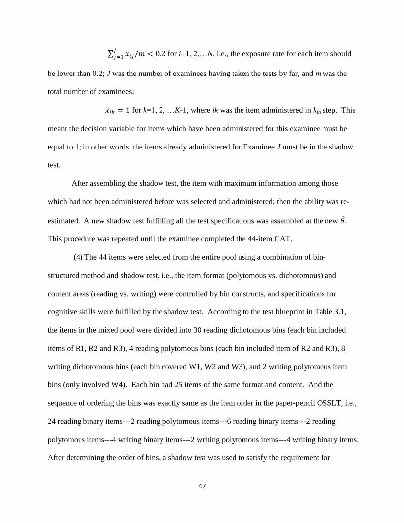
47
∑ for i=1, 2,…N, i.e., the exposure rate for each item should
be lower than 0.2; J was the number of examinees having taken the tests by far, and m was the
total number of examinees;
for k=1, 2, …K-1, where ik was the item administered in kth step. This
meant the decision variable for items which have been administered for this examinee must be
equal to 1; in other words, the items already administered for Examinee J must be in the shadow
test.
After assembling the shadow test, the item with maximum information among those
which had not been administered before was selected and administered; then the ability was re-
estimated. A new shadow test fulfilling all the test specifications was assembled at the new .
This procedure was repeated until the examinee completed the 44-item CAT.
(4) The 44 items were selected from the entire pool using a combination of bin-
structured method and shadow test, i.e., the item format (polytomous vs. dichotomous) and
content areas (reading vs. writing) were controlled by bin constructs, and specifications for
cognitive skills were fulfilled by the shadow test. According to the test blueprint in Table 3.1,
the items in the mixed pool were divided into 30 reading dichotomous bins (each bin included
items of R1, R2 and R3), 4 reading polytomous bins (each bin included item of R2 and R3), 8
writing dichotomous bins (each bin covered W1, W2 and W3), and 2 writing polytomous item
bins (only involved W4). Each bin had 25 items of the same format and content. And the
sequence of ordering the bins was exactly same as the item order in the paper-pencil OSSLT, i.e.,
24 reading binary items---2 reading polytomous items---6 reading binary items---2 reading
polytomous items---4 writing binary items---2 writing polytomous items---4 writing binary items.
After determining the order of bins, a shadow test was used to satisfy the requirement for
48
cognitive level, test information and exposure rate, but the shadow test only picked one item
from each bin in the order specified. In other words, besides the constraints in (3), one additional
constraint for shadow test was:
∑ , k=1, 2…44; i.e., draw one item from each bin.
(5) The 44 items were selected from the entire pool, but in contrast to (4), here bin
construct tool over the constraints on content area, item format, and also cognitive levels. The
entire mixed item pool was divided into 7 binary R1 bins, 17 binary R2 bins, 2 polytomous R2
bins, 6 binary R3 bins, 2 polytomous R3 bins, 2 binary W1 bins, 2 binary W2 bins, 4 binary W3
bins and 2 polytomous W4 bins. Each bin contained 25 items which were interchangeable with
respect to content, format and cognitive level. In other words, the number of bins in (5) was the
same as (4), but the criteria used to develop bins were different. And the order of bins was: 7
binary R1---17 binary R2---2 polytomous R2---6 binary R3---2 polytomous R3---2 binary W1---
2 binary W2---2 polytomous W4---4 binary W3, which was consistent with the OSSLT. A
shadow test was used to control exposure rate and achieve high test information; alternatively
speaking, the specifications for the shadow tests were:
Objective: maximize ∑ ( ) , i.e., maximize information at current ; N is the item
number in the whole item pool.
Constraints: ∑ , k=1, 2…44; i.e., draw one item from each bin;
∑ for i=1, 2,…N, i.e., the exposure rate for each item was
lower than 0.2; J was the number of examinees having taken the tests by far, and m was the total
number of examinees;
for k=1, 2, …K. where ik was the item administered in kth step. The
items which had already been administered must be in the shadow test.
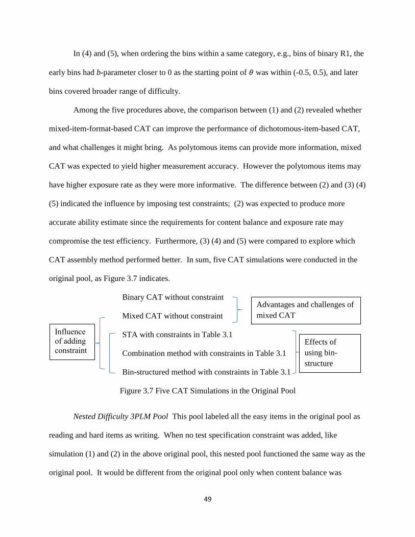
49
In (4) and (5), when ordering the bins within a same category, e.g., bins of binary R1, the
early bins had b-parameter closer to 0 as the starting point of was within (-0.5, 0.5), and later
bins covered broader range of difficulty.
Among the five procedures above, the comparison between (1) and (2) revealed whether
mixed-item-format-based CAT can improve the performance of dichotomous-item-based CAT,
and what challenges it might bring. As polytomous items can provide more information, mixed
CAT was expected to yield higher measurement accuracy. However the polytomous items may
have higher exposure rate as they were more informative. The difference between (2) and (3) (4)
(5) indicated the influence by imposing test constraints; (2) was expected to produce more
accurate ability estimate since the requirements for content balance and exposure rate may
compromise the test efficiency. Furthermore, (3) (4) and (5) were compared to explore which
CAT assembly method performed better. In sum, five CAT simulations were conducted in the
original pool, as Figure 3.7 indicates.
Binary CAT without constraint
Mixed CAT without constraint
STA with constraints in Table 3.1
Combination method with constraints in Table 3.1
Bin-structured method with constraints in Table 3.1
Figure 3.7 Five CAT Simulations in the Original Pool
Nested Difficulty 3PLM Pool This pool labeled all the easy items in the original pool as
reading and hard items as writing. When no test specification constraint was added, like
simulation (1) and (2) in the above original pool, this nested pool functioned the same way as the
original pool. It would be different from the original pool only when content balance was
Advantages and challenges of
mixed CAT
Effects of
using bin-
structure
Influence
of adding
constraint
s
50
required. Therefore three CATs were implemented using the nested difficulty 3PLM pool: (1)
shadow test with constraints in Table 3.1; (2) items were divided into 44 bins according to
format and content, while shadow test controlled the cognitive levels (as (4) in original pool);
and (3) items were divided into 44 bins according to format, content and cognitive levels (as (5)
in the original pool). For (2) and (3), the procedure of developing bins and the specifications for
the shadow test were same as the corresponding procedure in the original pool.
Recalibrated Pool The five CAT procedures in the original pool were repeated in the
recalibrated pool to explore the influence of adopting different IRT models. Each bin contained
25 items. In the original pool, the magnitude of b-parameter was used as a criterion to divide the
bins. In contrast, the recalibrated pool took a-parameters into consideration. When developing
the bins for the recalibrated pool, within a same bin category (e.g., for the binary reading bins),
the early bins had items with lower a-parameters, and later bins were more discriminative. This
strategy borrowed the idea of a-stratification design for CAT (Chang & Ying, 1999), which
states that in the early stage of CAT, the estimated ability may be far from the true ability, and
administering highly informative items at the beginning is a waste.
Nested Difficulty 2PLM Pool The three CAT procedures in the nested difficulty 3PLM
pool were repeated in this pool. Again, when developing the bins, later bins within a given item
category (e.g., binary R3) had higher a-parameters.
Balanced Item Pool The five procedures in original pool were conducted in the balanced
item pool to investigate the influence of pool shape. For a given bin category, early bins
contained items with lower a-parameters, while later bins had high a-parameters.
Heterogeneous Testlet Pool In all the pools above, the items within a testlet were
homogeneous and the testlet can be regarded as a polytomous item. However, in the
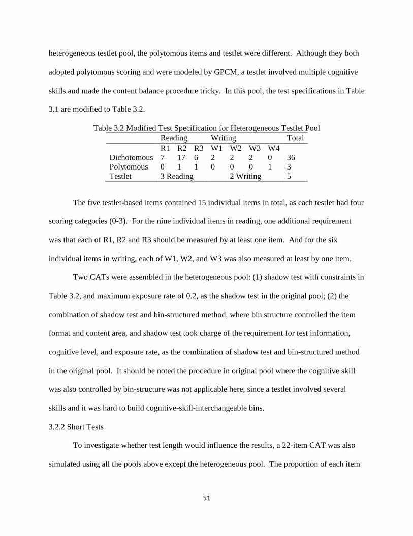
51
heterogeneous testlet pool, the polytomous items and testlet were different. Although they both
adopted polytomous scoring and were modeled by GPCM, a testlet involved multiple cognitive
skills and made the content balance procedure tricky. In this pool, the test specifications in Table
3.1 are modified to Table 3.2.
Table 3.2 Modified Test Specification for Heterogeneous Testlet Pool
Reading Writing Total
R1 R2 R3 W1 W2 W3 W4
Dichotomous 7 17 6 2 2 2 0 36
Polytomous 0 1 1 0 0 0 1 3
Testlet 3 Reading 2 Writing 5
The five testlet-based items contained 15 individual items in total, as each testlet had four
scoring categories (0-3). For the nine individual items in reading, one additional requirement
was that each of R1, R2 and R3 should be measured by at least one item. And for the six
individual items in writing, each of W1, W2, and W3 was also measured at least by one item.
Two CATs were assembled in the heterogeneous pool: (1) shadow test with constraints in
Table 3.2, and maximum exposure rate of 0.2, as the shadow test in the original pool; (2) the
combination of shadow test and bin-structured method, where bin structure controlled the item
format and content area, and shadow test took charge of the requirement for test information,
cognitive level, and exposure rate, as the combination of shadow test and bin-structured method
in the original pool. It should be noted the procedure in original pool where the cognitive skill
was also controlled by bin-structure was not applicable here, since a testlet involved several
skills and it was hard to build cognitive-skill-interchangeable bins.
3.2.2 Short Tests
To investigate whether test length would influence the results, a 22-item CAT was also
simulated using all the pools above except the heterogeneous pool. The proportion of each item

52
type is similar to the 44-item CAT, as Table 3.3 show. All the CAT procedures with long tests
were repeated with constraints in Table 3.3.
Table 3.3 Test Specification for 22-Item CAT
Reading Writing Total
R1 R2 R3 W1 W2 W3 W4
Dichotomous 3 9 3 1 1 2 0 19
Polytomous 0 1 1 0 0 0 1 3
In summary, two test lengths (44/22) * six item pools (original 3PLM/nested difficulty
3PLM/ recalibrated 2PLM/ nested difficulty 2PLM/ balanced/ heterogeneous testlet) * five CAT
assembly approaches (dichotomous only/ mixed format without constraint/shadow test/
combination of shadow test and bin-structured method/ pure bin-structured) were simulated. The
MOSEK package in Matlab was used to solve the optimal information problem. Each simulation
covered examinees with 81 evenly spaced ability within [-4, 4], and all simulations were
repeated 100 times.
3.3 Evaluation Criteria
Each testing simulation was evaluated by measurement, content, security, and item usage
efficiency criteria.
3.3.1 Measurement Criteria
Evaluation of measurement was based on overall and conditional results (Robin, 2008).
The overall statistics were obtained from all the 8100 (i.e., 81 ability levels *100 replications)
examinees. Conditional statistics were obtained from 100 replications at the given θ ability
levels. Both estimated indexes and true indexes were computed. Estimated standard errors of
measurement (SEM) were obtained through MLE and test information. Furthermore, since one
merit of the simulation study is the true value is known, the bias, mean absolute bias (MAB) and
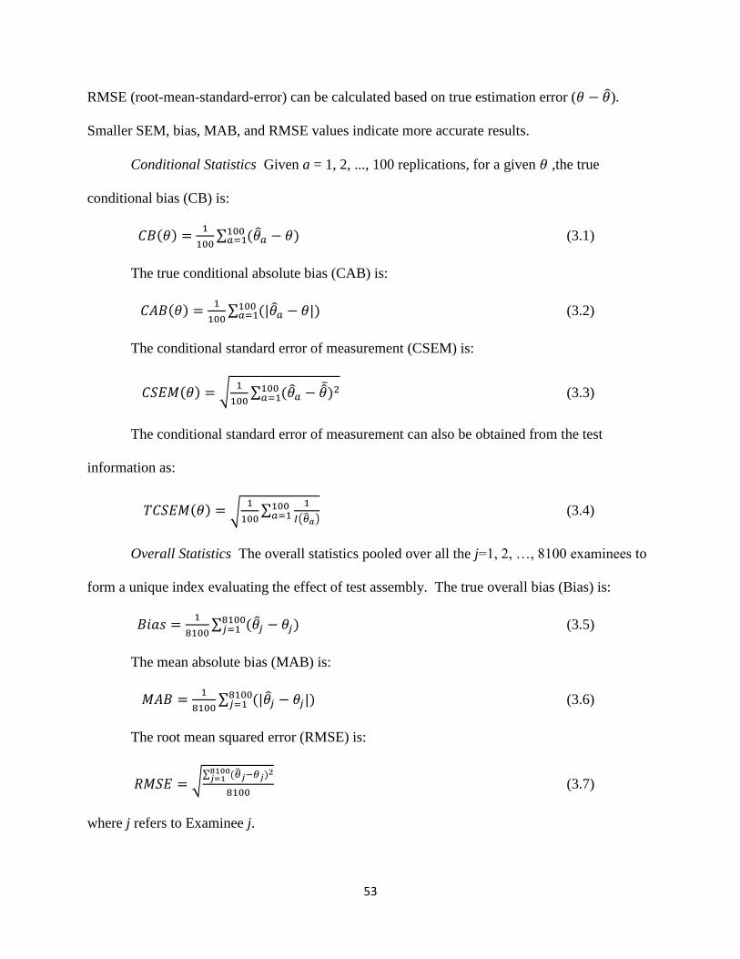
53
RMSE (root-mean-standard-error) can be calculated based on true estimation error ( ).
Smaller SEM, bias, MAB, and RMSE values indicate more accurate results.
Conditional Statistics Given a = 1, 2, ..., 100 replications, for a given ,the true
conditional bias (CB) is:
∑
(3.1)
The true conditional absolute bias (CAB) is:
∑
(3.2)
The conditional standard error of measurement (CSEM) is:
√
∑
(3.3)
The conditional standard error of measurement can also be obtained from the test
information as:
√
∑
( ) (3.4)
Overall Statistics The overall statistics pooled over all the j=1, 2, …, 8100 examinees to
form a unique index evaluating the effect of test assembly. The true overall bias (Bias) is:
∑
(3.5)
The mean absolute bias (MAB) is:
∑
(3.6)
The root mean squared error (RMSE) is:
√∑
(3.7)
where j refers to Examinee j.
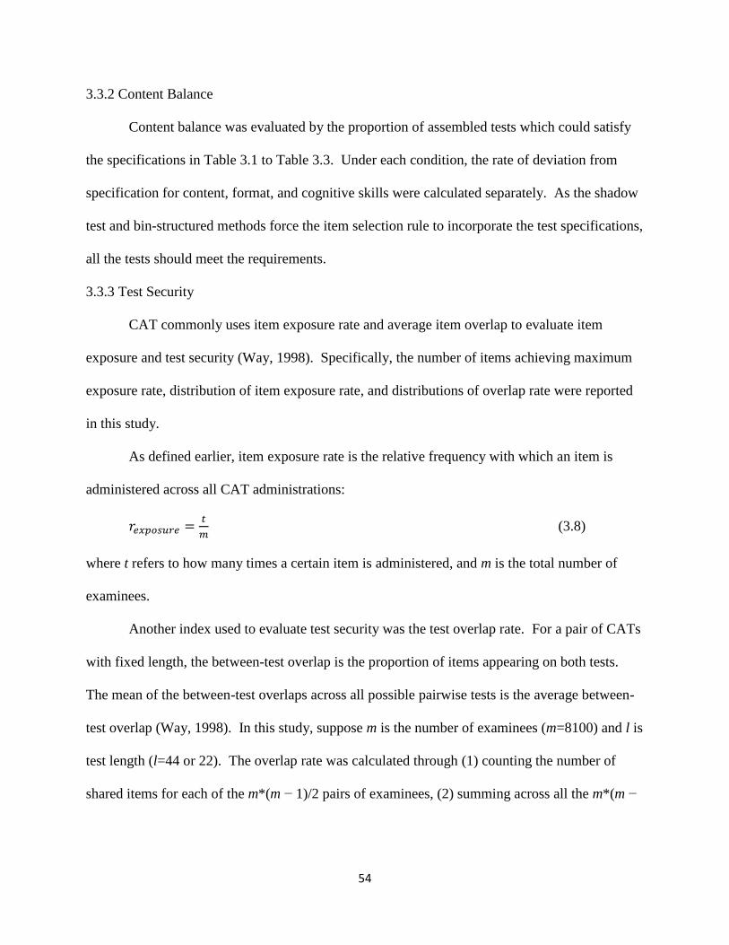
54
3.3.2 Content Balance
Content balance was evaluated by the proportion of assembled tests which could satisfy
the specifications in Table 3.1 to Table 3.3. Under each condition, the rate of deviation from
specification for content, format, and cognitive skills were calculated separately. As the shadow
test and bin-structured methods force the item selection rule to incorporate the test specifications,
all the tests should meet the requirements.
3.3.3 Test Security
CAT commonly uses item exposure rate and average item overlap to evaluate item
exposure and test security (Way, 1998). Specifically, the number of items achieving maximum
exposure rate, distribution of item exposure rate, and distributions of overlap rate were reported
in this study.
As defined earlier, item exposure rate is the relative frequency with which an item is
administered across all CAT administrations:
(3.8)
where t refers to how many times a certain item is administered, and m is the total number of
examinees.
Another index used to evaluate test security was the test overlap rate. For a pair of CATs
with fixed length, the between-test overlap is the proportion of items appearing on both tests.
The mean of the between-test overlaps across all possible pairwise tests is the average between-
test overlap (Way, 1998). In this study, suppose m is the number of examinees (m=8100) and l is
test length (l=44 or 22). The overlap rate was calculated through (1) counting the number of
shared items for each of the m*(m − 1)/2 pairs of examinees, (2) summing across all the m*(m −

55
1)/2 examinee pairs, and (3) dividing the total counts by l*m*(m − 1)/2. Small overlap rate
indicated higher security level.
3.3.4 Item Usage
The ideal item usage is achieved if all the items are utilized with equal frequency (Chang
& Ying, 1999). Therefore the distribution of item exposure rate and the number of never used
items can also measure the item pool usage efficiency.
56
Chapter 4: Results
This chapter summarizes the results of the simulation study described in Chapter 3. The
results are divided into two sections in response to the two research objectives proposed in
Chapter 1.
4.1 Research Question 1
To answer the question of whether the mixed CAT had advantages over the dichotomous-
item-based CAT, and what challenges the mixed CAT brought, the mixed CAT and dichotomous
CAT without any constraint were compared in measurement, test security and item pool usage
criteria. No content balance evaluation was conducted since no content constraint was added in
this case.
4.1.1 Measurement Criteria
The measurement criteria evaluated two facets of the CAT ability estimate: accuracy and
stability. While the conditional result demonstrates how findings vary across different ability
levels, the overall result can provide summary information about the effectiveness of each
method, and facilitates the interpretation (Robin, 2001). Therefore both overall and conditional
results are reported.
Conditional Result Information about bias and absolute bias indicates the accuracy,
while conditional standard error of measurement (CSEM) shows the variation of the estimate
around its mean and small value indicates a stable estimate. Test-information-based conditional
standard error of measurement (TCSEM) was also provided, which refers to the standard error of
measurement calculated through the test information and small value means high stability. The
difference between CSEM and TCSEM is: CSEM refers to the variation around the mean of
estimate, while TCSEM indicates the variation of the estimate around the true value; furthermore,
57
the TCSEM also assumes that the item parameters are true and the model fits the data well.
There was no obvious difference in conditional bias of ability estimate between the mixed and
dichotomous CAT, but at all ability levels, the mixed CAT had smaller absolute bias, CSEM,
TCSEM, and larger test information. See more details in Figure 4.1 (a)-(k) to Figure 4.5(a)-(k).
Overall Result Compared with the dichotomous CAT, the mixed CAT had smaller mean
bias, mean absolute bias, and RMSE under all simulation conditions. See more details in Table
4.1 to 4.3.
4.1.2 Test Security Criteria
Item Exposure The mixed CAT had more skewed item exposure rate distribution than
the dichotomous CAT. In the mixed CAT, several items were administered to most of the
examinees, while almost 90% of the items were never used. Further analysis showed that in the
mixed CAT the items with highest exposure rate were all polytomously scored items. See more
details in Figure 4.6 to 4.10.
Overlap Rate The mixed CAT had higher overall overlap rate. Also, along the whole
ability continuum, it had higher conditional overlap rate than the dichotomous CAT. See more
details in Figure 4.12(a)-(k) and Table 4.5.
4.1.3 Item Usage
Since the more skewed item exposure rate distribution indicates less efficiency, the
efficiency of item usage was lower in the mixed CAT than in the dichotomous CAT.
Furthermore, under most circumstances more than 85% of the items in the mixed CAT were
never used. See more details in Table 4.6.
In sum, the mixed CAT can lead to higher measurement accuracy and stability, in terms
of both overall and conditional index. However, it had higher overlap rate and more highly
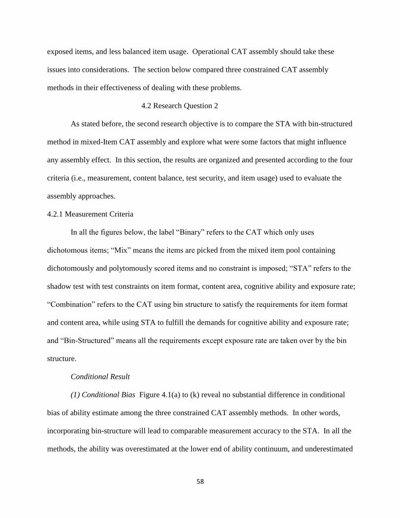
58
exposed items, and less balanced item usage. Operational CAT assembly should take these
issues into considerations. The section below compared three constrained CAT assembly
methods in their effectiveness of dealing with these problems.
4.2 Research Question 2
As stated before, the second research objective is to compare the STA with bin-structured
method in mixed-Item CAT assembly and explore what were some factors that might influence
any assembly effect. In this section, the results are organized and presented according to the four
criteria (i.e., measurement, content balance, test security, and item usage) used to evaluate the
assembly approaches.
4.2.1 Measurement Criteria
In all the figures below, the label “Binary” refers to the CAT which only uses
dichotomous items; “Mix” means the items are picked from the mixed item pool containing
dichotomously and polytomously scored items and no constraint is imposed; “STA” refers to the
shadow test with test constraints on item format, content area, cognitive ability and exposure rate;
“Combination” refers to the CAT using bin structure to satisfy the requirements for item format
and content area, while using STA to fulfill the demands for cognitive ability and exposure rate;
and “Bin-Structured” means all the requirements except exposure rate are taken over by the bin
structure.
Conditional Result
(1) Conditional Bias Figure 4.1(a) to (k) reveal no substantial difference in conditional
bias of ability estimate among the three constrained CAT assembly methods. In other words,
incorporating bin-structure will lead to comparable measurement accuracy to the STA. In all the
methods, the ability was overestimated at the lower end of ability continuum, and underestimated
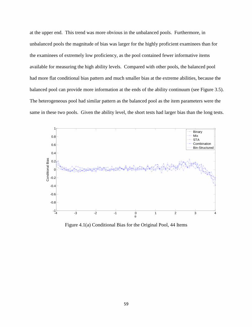
59
at the upper end. This trend was more obvious in the unbalanced pools. Furthermore, in
unbalanced pools the magnitude of bias was larger for the highly proficient examinees than for
the examinees of extremely low proficiency, as the pool contained fewer informative items
available for measuring the high ability levels. Compared with other pools, the balanced pool
had more flat conditional bias pattern and much smaller bias at the extreme abilities, because the
balanced pool can provide more information at the ends of the ability continuum (see Figure 3.5).
The heterogeneous pool had similar pattern as the balanced pool as the item parameters were the
same in these two pools. Given the ability level, the short tests had larger bias than the long tests.
Figure 4.1(a) Conditional Bias for the Original Pool, 44 Items
-4 -3 -2 -1 0 1 2 3 4-1
-0.8
-0.6
-0.4
-0.2
0
0.2
0.4
0.6
0.8
1
Co
nd
itio
nal B
ias
Binary
Mix
STA
Combination
Bin-Structured
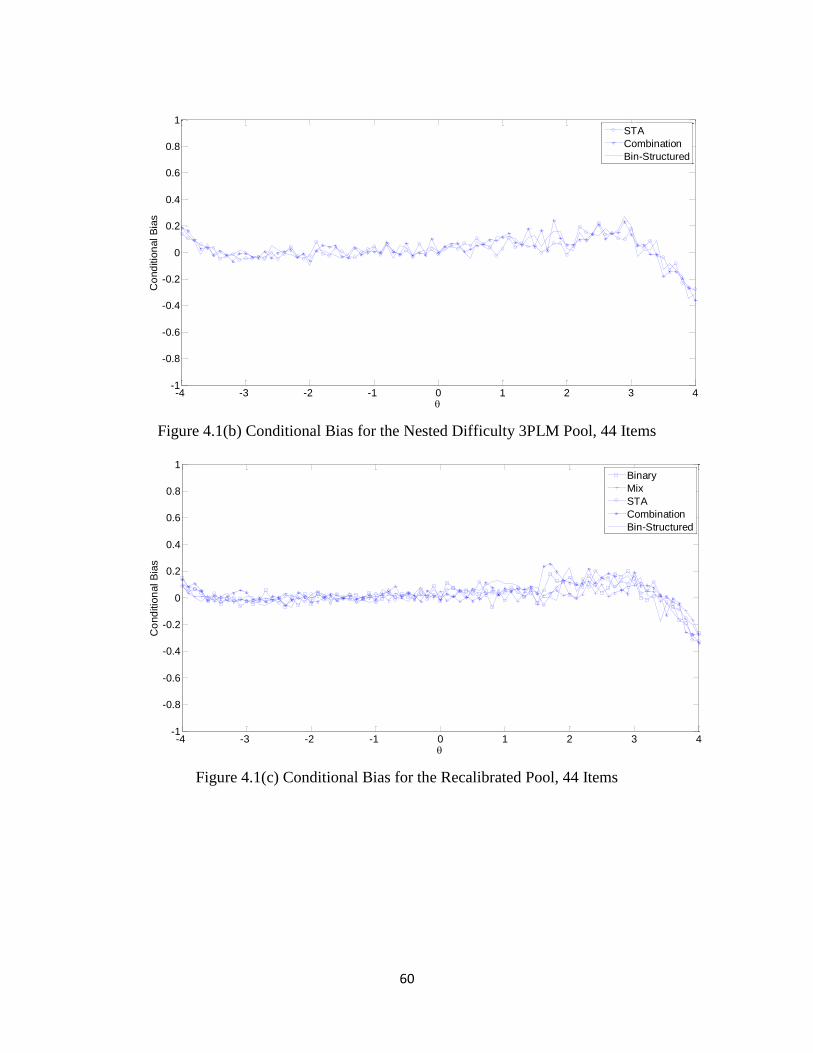
60
Figure 4.1(b) Conditional Bias for the Nested Difficulty 3PLM Pool, 44 Items
Figure 4.1(c) Conditional Bias for the Recalibrated Pool, 44 Items
-4 -3 -2 -1 0 1 2 3 4-1
-0.8
-0.6
-0.4
-0.2
0
0.2
0.4
0.6
0.8
1
Co
nd
itio
nal B
ias
STA
Combination
Bin-Structured
-4 -3 -2 -1 0 1 2 3 4-1
-0.8
-0.6
-0.4
-0.2
0
0.2
0.4
0.6
0.8
1
Co
nd
itio
nal B
ias
Binary
Mix
STA
Combination
Bin-Structured
61
Figure 4.1(d) Conditional Bias for the Nested Difficulty 2PLM Pool, 44 Items
Figure 4.1(e) Conditional Bias for the Balanced Pool, 44 Items
-4 -3 -2 -1 0 1 2 3 4-1
-0.8
-0.6
-0.4
-0.2
0
0.2
0.4
0.6
0.8
1
Co
nd
itio
nal B
ias
STA
Combination
Bin-Structured
-4 -3 -2 -1 0 1 2 3 4-1
-0.8
-0.6
-0.4
-0.2
0
0.2
0.4
0.6
0.8
1
Co
nd
itio
nal B
ias
Binary
Mix
STA
Combination
Bin-Structured
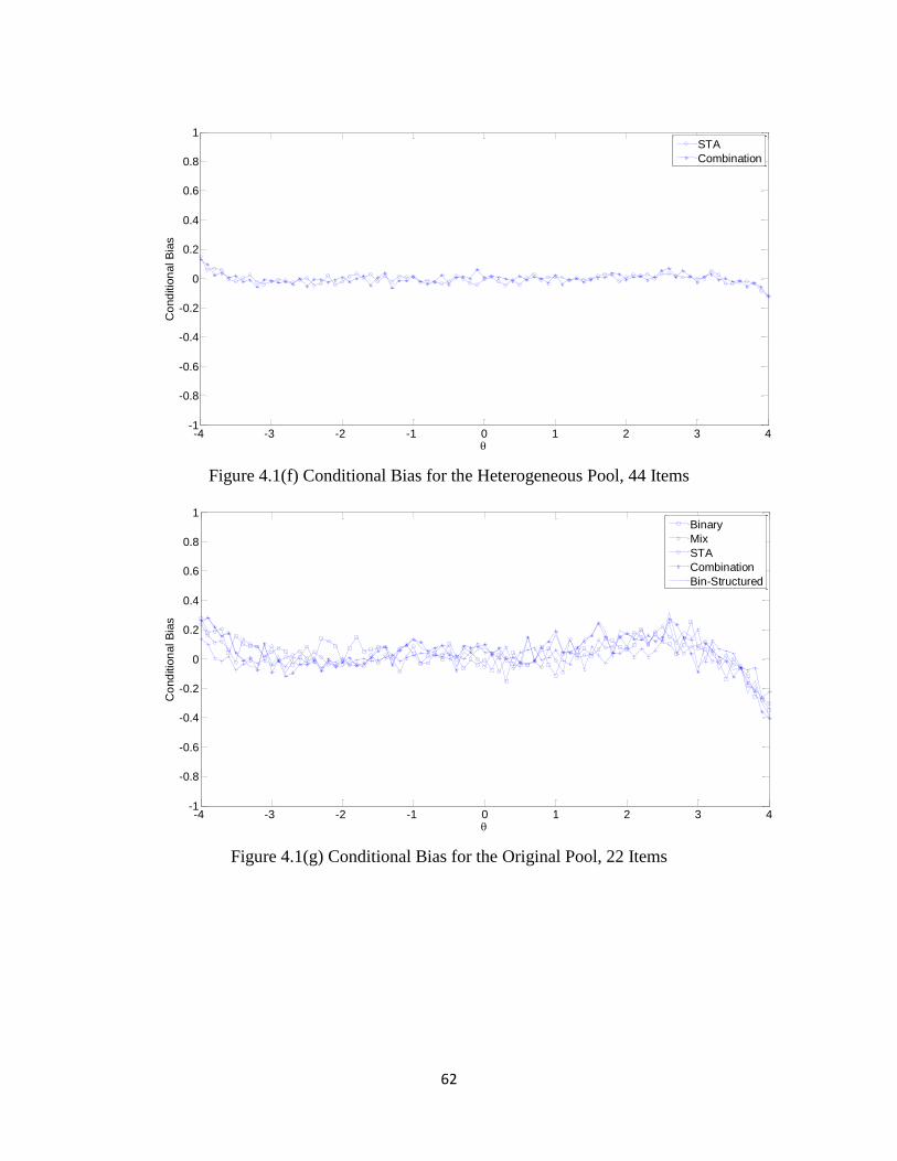
62
Figure 4.1(f) Conditional Bias for the Heterogeneous Pool, 44 Items
Figure 4.1(g) Conditional Bias for the Original Pool, 22 Items
-4 -3 -2 -1 0 1 2 3 4-1
-0.8
-0.6
-0.4
-0.2
0
0.2
0.4
0.6
0.8
1
Co
nd
itio
nal B
ias
STA
Combination
-4 -3 -2 -1 0 1 2 3 4-1
-0.8
-0.6
-0.4
-0.2
0
0.2
0.4
0.6
0.8
1
Co
nd
itio
nal B
ias
Binary
Mix
STA
Combination
Bin-Structured
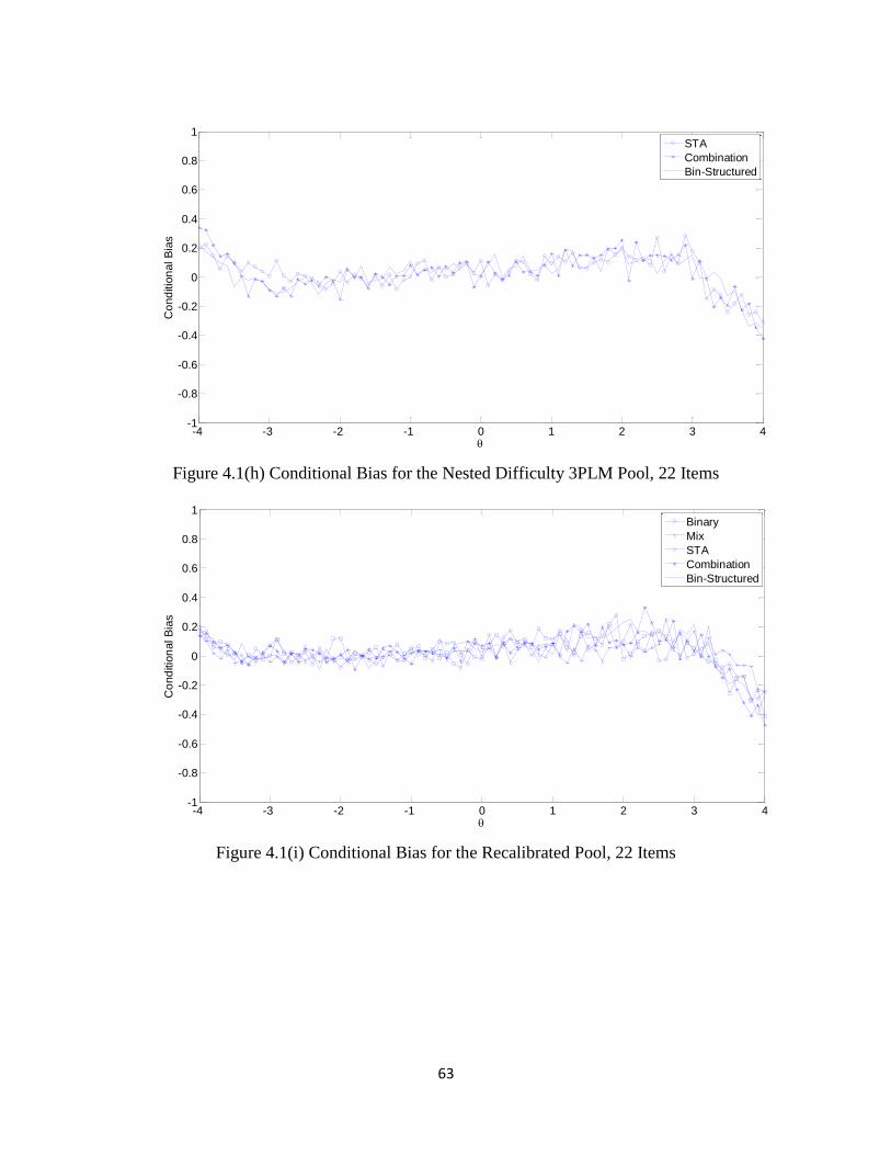
63
Figure 4.1(h) Conditional Bias for the Nested Difficulty 3PLM Pool, 22 Items
Figure 4.1(i) Conditional Bias for the Recalibrated Pool, 22 Items
-4 -3 -2 -1 0 1 2 3 4-1
-0.8
-0.6
-0.4
-0.2
0
0.2
0.4
0.6
0.8
1
Co
nd
itio
nal B
ias
STA
Combination
Bin-Structured
-4 -3 -2 -1 0 1 2 3 4-1
-0.8
-0.6
-0.4
-0.2
0
0.2
0.4
0.6
0.8
1
Co
nd
itio
nal B
ias
Binary
Mix
STA
Combination
Bin-Structured
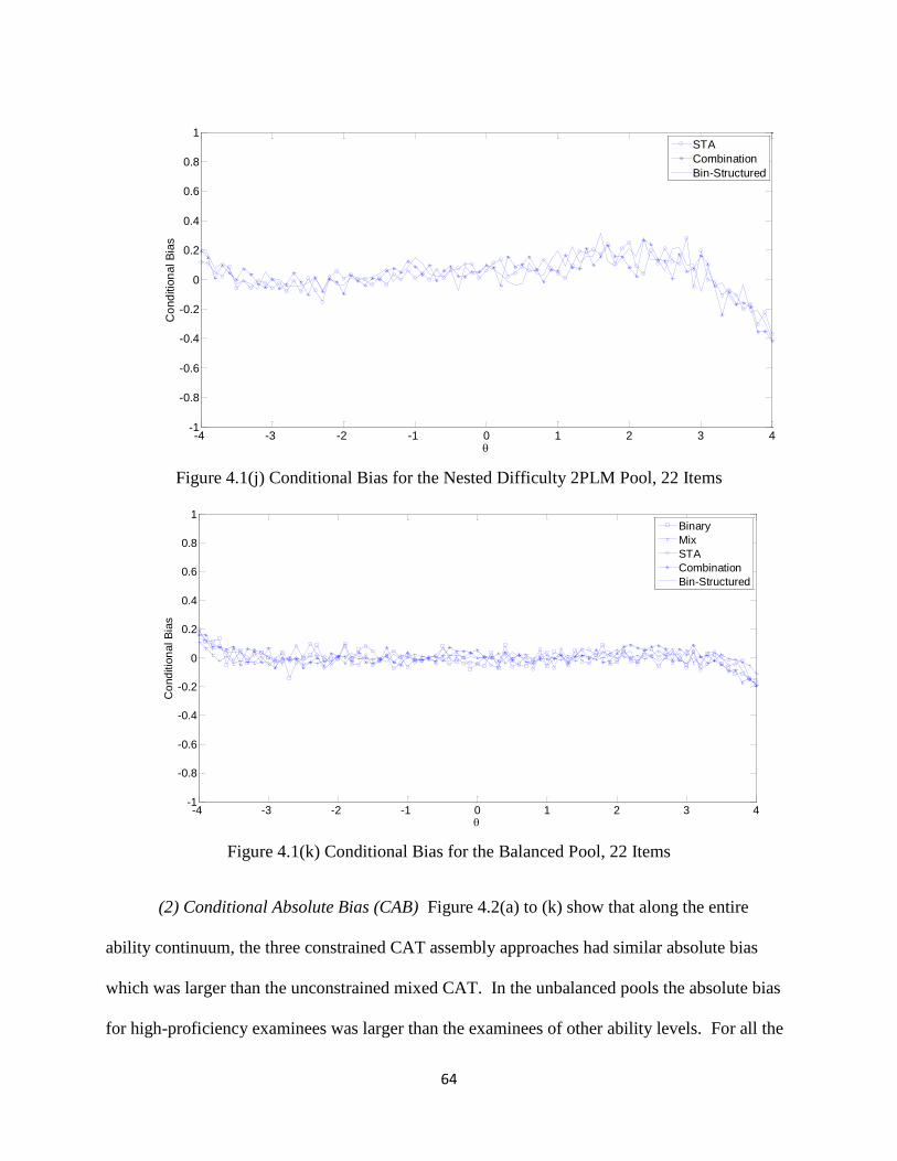
64
Figure 4.1(j) Conditional Bias for the Nested Difficulty 2PLM Pool, 22 Items
Figure 4.1(k) Conditional Bias for the Balanced Pool, 22 Items
(2) Conditional Absolute Bias (CAB) Figure 4.2(a) to (k) show that along the entire
ability continuum, the three constrained CAT assembly approaches had similar absolute bias
which was larger than the unconstrained mixed CAT. In the unbalanced pools the absolute bias
for high-proficiency examinees was larger than the examinees of other ability levels. For all the
-4 -3 -2 -1 0 1 2 3 4-1
-0.8
-0.6
-0.4
-0.2
0
0.2
0.4
0.6
0.8
1
Co
nd
itio
nal B
ias
STA
Combination
Bin-Structured
-4 -3 -2 -1 0 1 2 3 4-1
-0.8
-0.6
-0.4
-0.2
0
0.2
0.4
0.6
0.8
1
Co
nd
itio
nal B
ias
Binary
Mix
STA
Combination
Bin-Structured
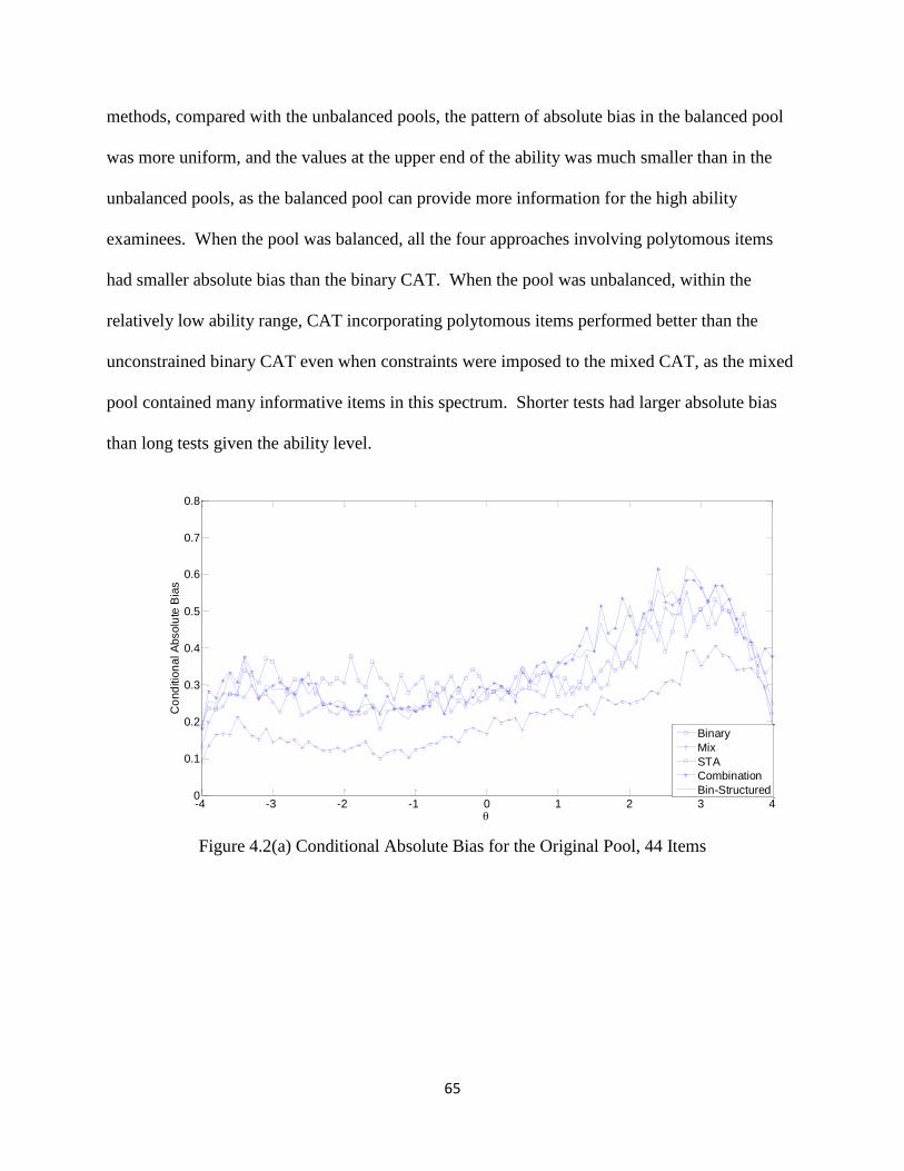
65
methods, compared with the unbalanced pools, the pattern of absolute bias in the balanced pool
was more uniform, and the values at the upper end of the ability was much smaller than in the
unbalanced pools, as the balanced pool can provide more information for the high ability
examinees. When the pool was balanced, all the four approaches involving polytomous items
had smaller absolute bias than the binary CAT. When the pool was unbalanced, within the
relatively low ability range, CAT incorporating polytomous items performed better than the
unconstrained binary CAT even when constraints were imposed to the mixed CAT, as the mixed
pool contained many informative items in this spectrum. Shorter tests had larger absolute bias
than long tests given the ability level.
Figure 4.2(a) Conditional Absolute Bias for the Original Pool, 44 Items
-4 -3 -2 -1 0 1 2 3 40
0.1
0.2
0.3
0.4
0.5
0.6
0.7
0.8
Co
nd
itio
nal A
bsolu
te B
ias
Binary
Mix
STA
Combination
Bin-Structured
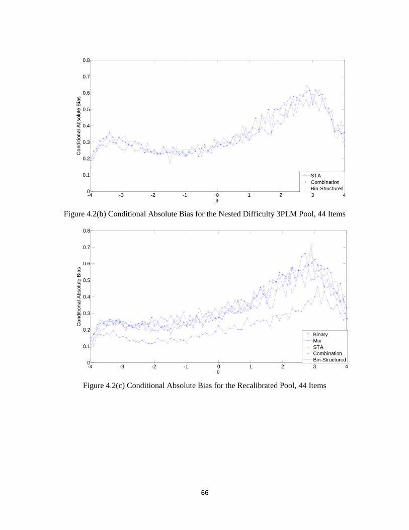
66
Figure 4.2(b) Conditional Absolute Bias for the Nested Difficulty 3PLM Pool, 44 Items
Figure 4.2(c) Conditional Absolute Bias for the Recalibrated Pool, 44 Items
-4 -3 -2 -1 0 1 2 3 40
0.1
0.2
0.3
0.4
0.5
0.6
0.7
0.8
Co
nd
itio
nal A
bsolu
te B
ias
STA
Combination
Bin-Structured
-4 -3 -2 -1 0 1 2 3 40
0.1
0.2
0.3
0.4
0.5
0.6
0.7
0.8
Co
nd
itio
nal A
bsolu
te B
ias
Binary
Mix
STA
Combination
Bin-Structured
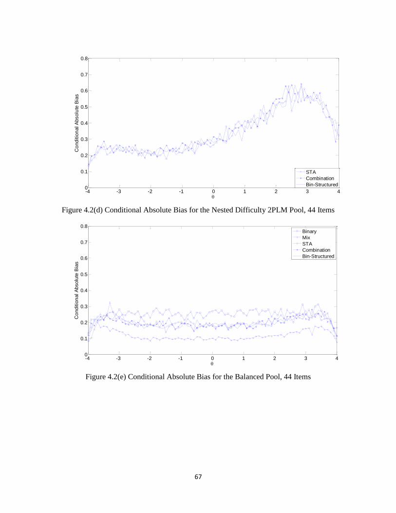
67
Figure 4.2(d) Conditional Absolute Bias for the Nested Difficulty 2PLM Pool, 44 Items
Figure 4.2(e) Conditional Absolute Bias for the Balanced Pool, 44 Items
-4 -3 -2 -1 0 1 2 3 40
0.1
0.2
0.3
0.4
0.5
0.6
0.7
0.8
Co
nd
itio
nal A
bsolu
te B
ias
STA
Combination
Bin-Structured
-4 -3 -2 -1 0 1 2 3 40
0.1
0.2
0.3
0.4
0.5
0.6
0.7
0.8
Co
nd
itio
nal A
bsolu
te B
ias
Binary
Mix
STA
Combination
Bin-Structured
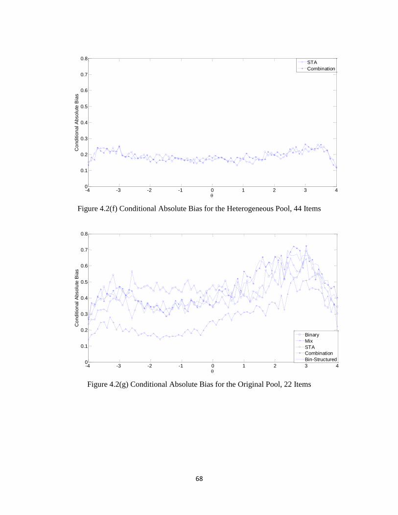
68
Figure 4.2(f) Conditional Absolute Bias for the Heterogeneous Pool, 44 Items
Figure 4.2(g) Conditional Absolute Bias for the Original Pool, 22 Items
-4 -3 -2 -1 0 1 2 3 40
0.1
0.2
0.3
0.4
0.5
0.6
0.7
0.8
Co
nd
itio
nal A
bsolu
te B
ias
STA
Combination
-4 -3 -2 -1 0 1 2 3 40
0.1
0.2
0.3
0.4
0.5
0.6
0.7
0.8
Co
nd
itio
nal A
bsolu
te B
ias
Binary
Mix
STA
Combination
Bin-Structured
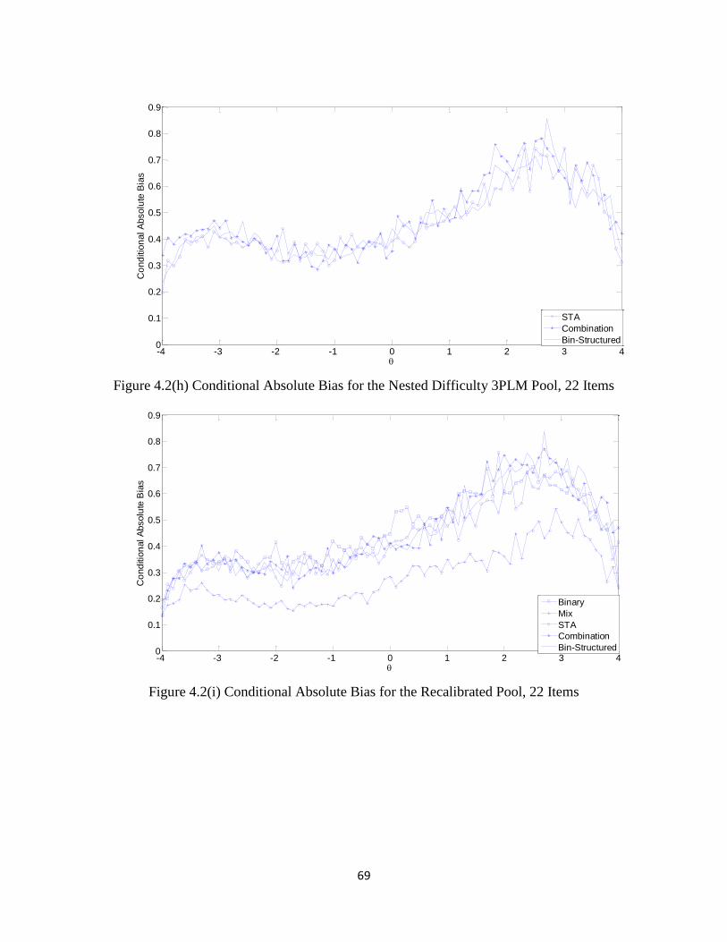
69
Figure 4.2(h) Conditional Absolute Bias for the Nested Difficulty 3PLM Pool, 22 Items
Figure 4.2(i) Conditional Absolute Bias for the Recalibrated Pool, 22 Items
-4 -3 -2 -1 0 1 2 3 40
0.1
0.2
0.3
0.4
0.5
0.6
0.7
0.8
0.9
Co
nd
itio
nal A
bsolu
te B
ias
STA
Combination
Bin-Structured
-4 -3 -2 -1 0 1 2 3 40
0.1
0.2
0.3
0.4
0.5
0.6
0.7
0.8
0.9
Co
nd
itio
nal A
bsolu
te B
ias
Binary
Mix
STA
Combination
Bin-Structured
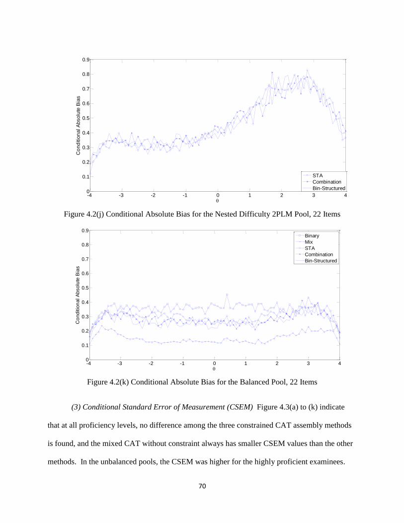
70
Figure 4.2(j) Conditional Absolute Bias for the Nested Difficulty 2PLM Pool, 22 Items
Figure 4.2(k) Conditional Absolute Bias for the Balanced Pool, 22 Items
(3) Conditional Standard Error of Measurement (CSEM) Figure 4.3(a) to (k) indicate
that at all proficiency levels, no difference among the three constrained CAT assembly methods
is found, and the mixed CAT without constraint always has smaller CSEM values than the other
methods. In the unbalanced pools, the CSEM was higher for the highly proficient examinees.
-4 -3 -2 -1 0 1 2 3 40
0.1
0.2
0.3
0.4
0.5
0.6
0.7
0.8
0.9
Co
nd
itio
nal A
bsolu
te B
ias
STA
Combination
Bin-Structured
-4 -3 -2 -1 0 1 2 3 40
0.1
0.2
0.3
0.4
0.5
0.6
0.7
0.8
0.9
Co
nd
itio
nal A
bsolu
te B
ias
Binary
Mix
STA
Combination
Bin-Structured
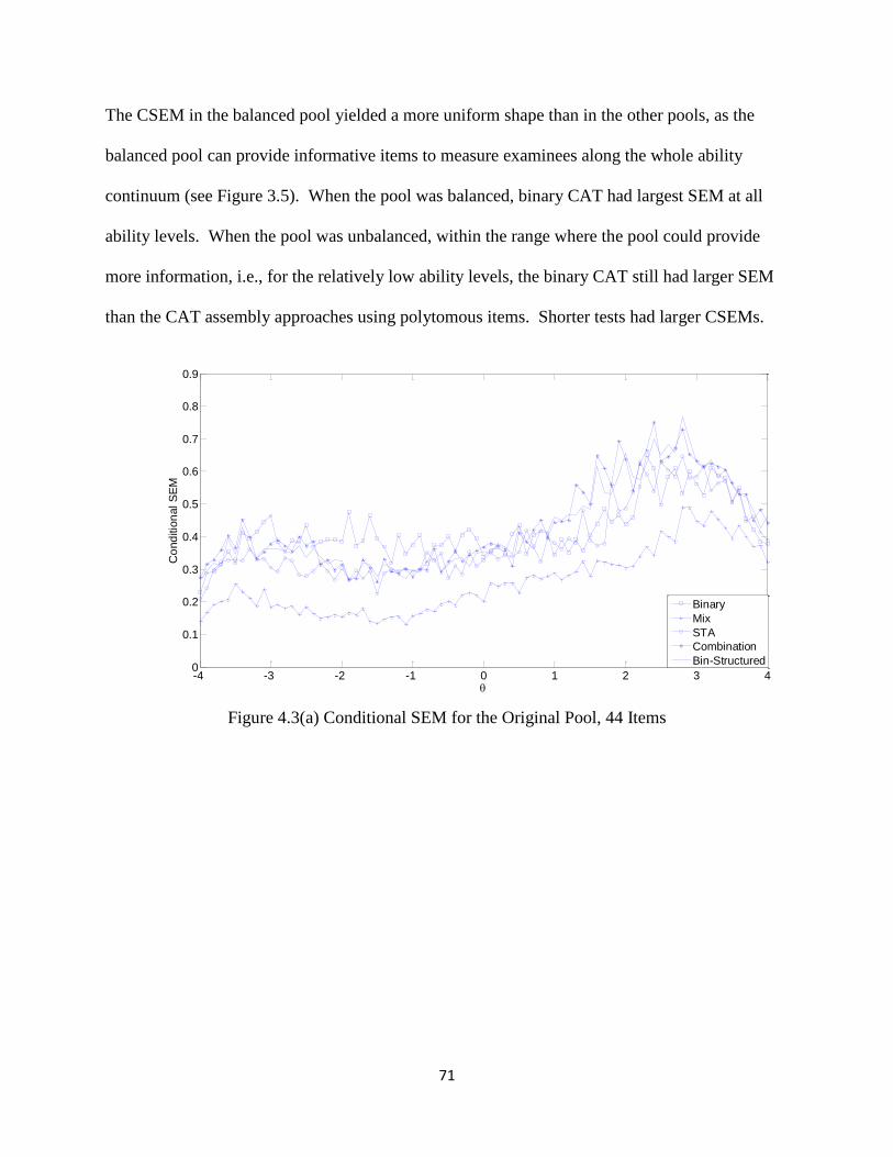
71
The CSEM in the balanced pool yielded a more uniform shape than in the other pools, as the
balanced pool can provide informative items to measure examinees along the whole ability
continuum (see Figure 3.5). When the pool was balanced, binary CAT had largest SEM at all
ability levels. When the pool was unbalanced, within the range where the pool could provide
more information, i.e., for the relatively low ability levels, the binary CAT still had larger SEM
than the CAT assembly approaches using polytomous items. Shorter tests had larger CSEMs.
Figure 4.3(a) Conditional SEM for the Original Pool, 44 Items
-4 -3 -2 -1 0 1 2 3 40
0.1
0.2
0.3
0.4
0.5
0.6
0.7
0.8
0.9
Co
nd
itio
nal S
EM
Binary
Mix
STA
Combination
Bin-Structured
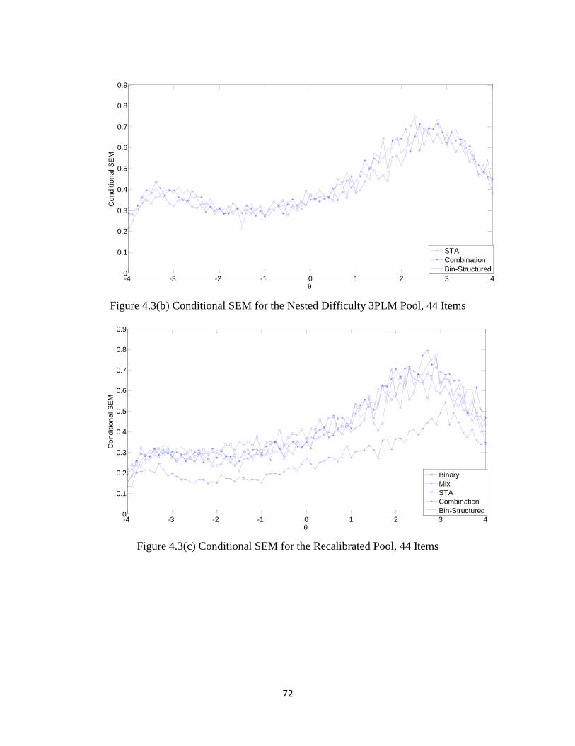
72
Figure 4.3(b) Conditional SEM for the Nested Difficulty 3PLM Pool, 44 Items
Figure 4.3(c) Conditional SEM for the Recalibrated Pool, 44 Items
-4 -3 -2 -1 0 1 2 3 40
0.1
0.2
0.3
0.4
0.5
0.6
0.7
0.8
0.9
Co
nd
itio
nal S
EM
STA
Combination
Bin-Structured
-4 -3 -2 -1 0 1 2 3 40
0.1
0.2
0.3
0.4
0.5
0.6
0.7
0.8
0.9
Co
nd
itio
nal S
EM
Binary
Mix
STA
Combination
Bin-Structured
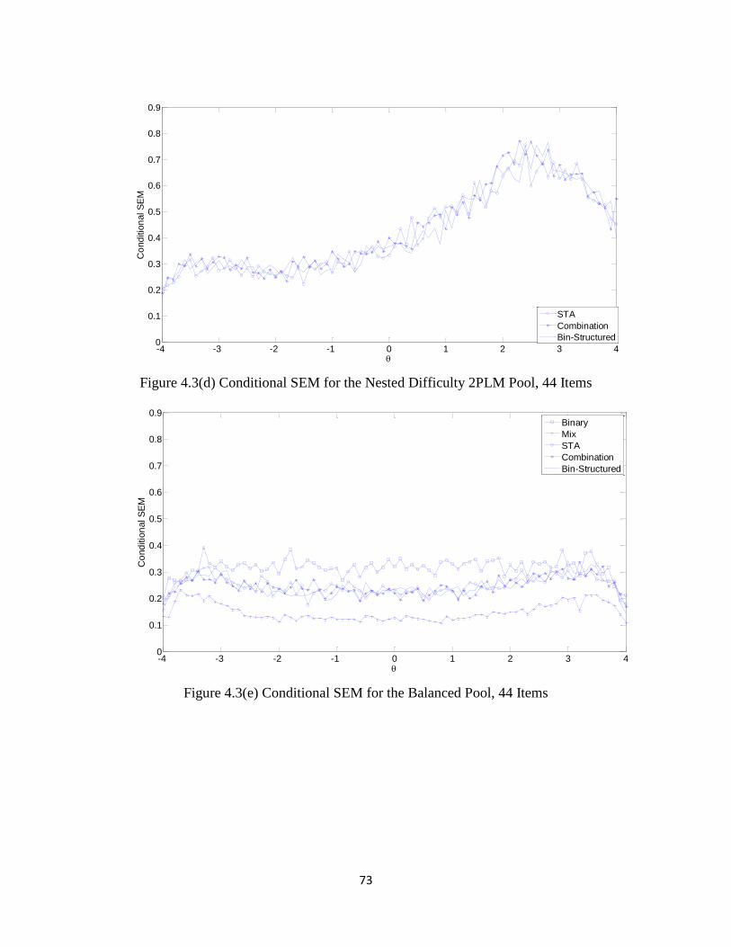
73
Figure 4.3(d) Conditional SEM for the Nested Difficulty 2PLM Pool, 44 Items
Figure 4.3(e) Conditional SEM for the Balanced Pool, 44 Items
-4 -3 -2 -1 0 1 2 3 40
0.1
0.2
0.3
0.4
0.5
0.6
0.7
0.8
0.9
Co
nd
itio
nal S
EM
STA
Combination
Bin-Structured
-4 -3 -2 -1 0 1 2 3 40
0.1
0.2
0.3
0.4
0.5
0.6
0.7
0.8
0.9
Co
nd
itio
nal S
EM
Binary
Mix
STA
Combination
Bin-Structured
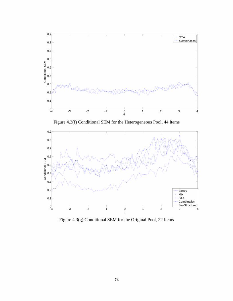
74
Figure 4.3(f) Conditional SEM for the Heterogeneous Pool, 44 Items
Figure 4.3(g) Conditional SEM for the Original Pool, 22 Items
-4 -3 -2 -1 0 1 2 3 40
0.1
0.2
0.3
0.4
0.5
0.6
0.7
0.8
0.9
Co
nd
itio
nal S
EM
STA
Combination
-4 -3 -2 -1 0 1 2 3 40
0.1
0.2
0.3
0.4
0.5
0.6
0.7
0.8
0.9
Co
nd
itio
nal S
EM
Binary
Mix
STA
Combination
Bin-Structured
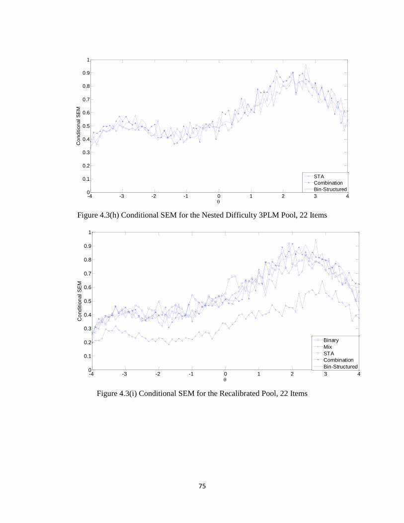
75
Figure 4.3(h) Conditional SEM for the Nested Difficulty 3PLM Pool, 22 Items
Figure 4.3(i) Conditional SEM for the Recalibrated Pool, 22 Items
-4 -3 -2 -1 0 1 2 3 40
0.1
0.2
0.3
0.4
0.5
0.6
0.7
0.8
0.9
1
Co
nd
itio
nal S
EM
STA
Combination
Bin-Structured
-4 -3 -2 -1 0 1 2 3 40
0.1
0.2
0.3
0.4
0.5
0.6
0.7
0.8
0.9
1
Co
nd
itio
nal S
EM
Binary
Mix
STA
Combination
Bin-Structured
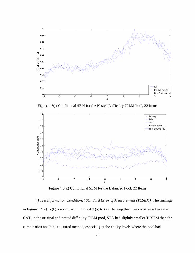
76
Figure 4.3(j) Conditional SEM for the Nested Difficulty 2PLM Pool, 22 Items
Figure 4.3(k) Conditional SEM for the Balanced Pool, 22 Items
(4) Test Information Conditional Standard Error of Measurement (TCSEM) The findings
in Figure 4.4(a) to (k) are similar to Figure 4.3 (a) to (k). Among the three constrained mixed-
CAT, in the original and nested difficulty 3PLM pool, STA had slightly smaller TCSEM than the
combination and bin-structured method, especially at the ability levels where the pool had
-4 -3 -2 -1 0 1 2 3 40
0.1
0.2
0.3
0.4
0.5
0.6
0.7
0.8
0.9
1
Co
nd
itio
nal S
EM
STA
Combination
Bin-Structured
-4 -3 -2 -1 0 1 2 3 40
0.1
0.2
0.3
0.4
0.5
0.6
0.7
0.8
0.9
1
Co
nd
itio
nal S
EM
Binary
Mix
STA
Combination
Bin-Structured
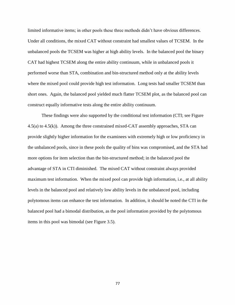
77
limited informative items; in other pools these three methods didn’t have obvious differences.
Under all conditions, the mixed CAT without constraint had smallest values of TCSEM. In the
unbalanced pools the TCSEM was higher at high ability levels. In the balanced pool the binary
CAT had highest TCSEM along the entire ability continuum, while in unbalanced pools it
performed worse than STA, combination and bin-structured method only at the ability levels
where the mixed pool could provide high test information. Long tests had smaller TCSEM than
short ones. Again, the balanced pool yielded much flatter TCSEM plot, as the balanced pool can
construct equally informative tests along the entire ability continuum.
These findings were also supported by the conditional test information (CTI; see Figure
4.5(a) to 4.5(k)). Among the three constrained mixed-CAT assembly approaches, STA can
provide slightly higher information for the examinees with extremely high or low proficiency in
the unbalanced pools, since in these pools the quality of bins was compromised, and the STA had
more options for item selection than the bin-structured method; in the balanced pool the
advantage of STA in CTI diminished. The mixed CAT without constraint always provided
maximum test information. When the mixed pool can provide high information, i.e., at all ability
levels in the balanced pool and relatively low ability levels in the unbalanced pool, including
polytomous items can enhance the test information. In addition, it should be noted the CTI in the
balanced pool had a bimodal distribution, as the pool information provided by the polytomous
items in this pool was bimodal (see Figure 3.5).

78
Figure 4.4(a) TCSEM for the Original Pool, 44 Items
Figure 4.4(b) TCSEM for the Nested Difficulty 3PLM Pool, 44 Items
-4 -3 -2 -1 0 1 2 3 40
0.1
0.2
0.3
0.4
0.5
0.6
0.7
0.8
0.9
1
TC
SE
M
Binary
Mix
STA
Combination
Bin-Structured
-4 -3 -2 -1 0 1 2 3 40
0.1
0.2
0.3
0.4
0.5
0.6
0.7
0.8
0.9
1
TC
SE
M
STA
Combination
Bin-Structured
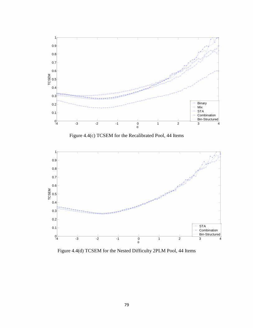
79
Figure 4.4(c) TCSEM for the Recalibrated Pool, 44 Items
Figure 4.4(d) TCSEM for the Nested Difficulty 2PLM Pool, 44 Items
-4 -3 -2 -1 0 1 2 3 40
0.1
0.2
0.3
0.4
0.5
0.6
0.7
0.8
0.9
1
TC
SE
M
Binary
Mix
STA
Combination
Bin-Structured
-4 -3 -2 -1 0 1 2 3 40
0.1
0.2
0.3
0.4
0.5
0.6
0.7
0.8
0.9
1
TC
SE
M
STA
Combination
Bin-Structured
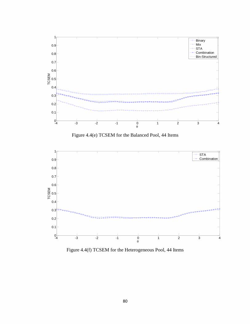
80
Figure 4.4(e) TCSEM for the Balanced Pool, 44 Items
Figure 4.4(f) TCSEM for the Heterogeneous Pool, 44 Items
-4 -3 -2 -1 0 1 2 3 40
0.1
0.2
0.3
0.4
0.5
0.6
0.7
0.8
0.9
1
TC
SE
M
Binary
Mix
STA
Combination
Bin-Structured
-4 -3 -2 -1 0 1 2 3 40
0.1
0.2
0.3
0.4
0.5
0.6
0.7
0.8
0.9
1
TC
SE
M
STA
Combination
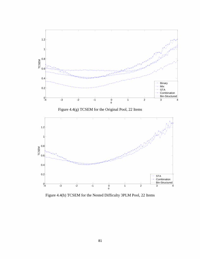
81
Figure 4.4(g) TCSEM for the Original Pool, 22 Items
Figure 4.4(h) TCSEM for the Nested Difficulty 3PLM Pool, 22 Items
-4 -3 -2 -1 0 1 2 3 40
0.2
0.4
0.6
0.8
1
1.2
TC
SE
M
Binary
Mix
STA
Combination
Bin-Structured
-4 -3 -2 -1 0 1 2 3 40
0.2
0.4
0.6
0.8
1
1.2
TC
SE
M
STA
Combination
Bin-Structured
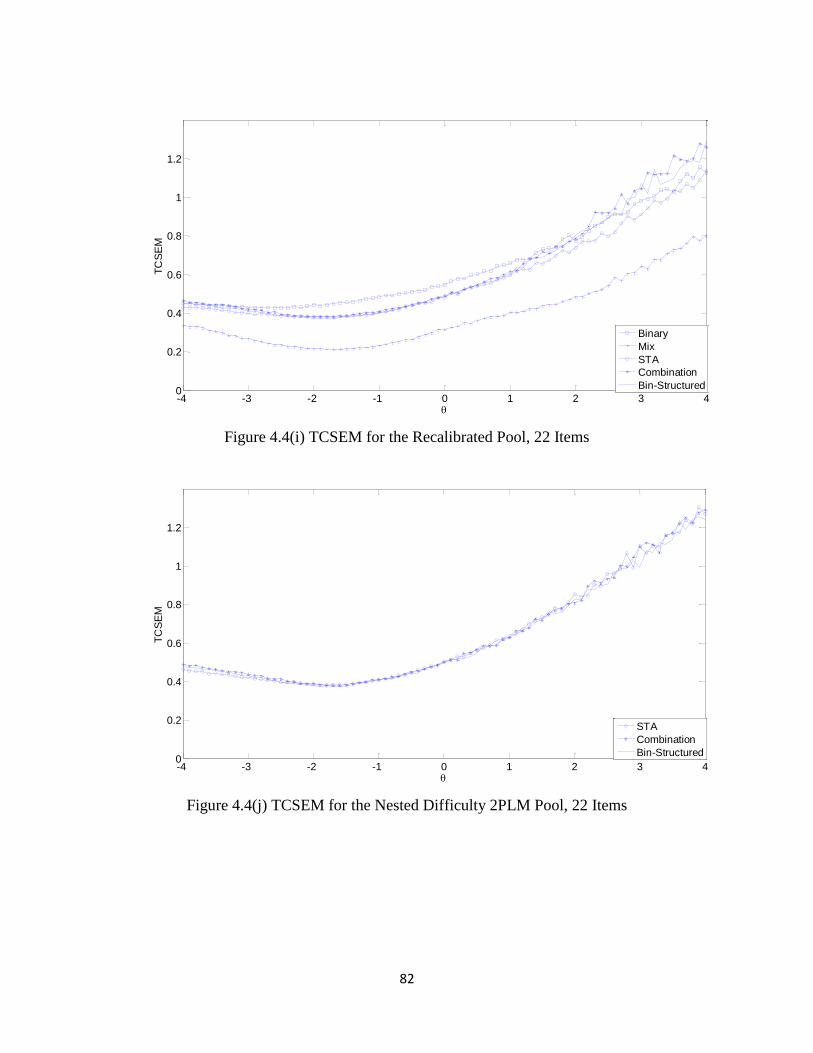
82
Figure 4.4(i) TCSEM for the Recalibrated Pool, 22 Items
Figure 4.4(j) TCSEM for the Nested Difficulty 2PLM Pool, 22 Items
-4 -3 -2 -1 0 1 2 3 40
0.2
0.4
0.6
0.8
1
1.2
TC
SE
M
Binary
Mix
STA
Combination
Bin-Structured
-4 -3 -2 -1 0 1 2 3 40
0.2
0.4
0.6
0.8
1
1.2
TC
SE
M
STA
Combination
Bin-Structured
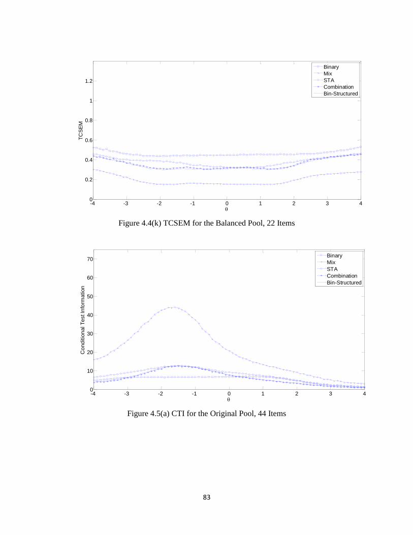
83
Figure 4.4(k) TCSEM for the Balanced Pool, 22 Items
Figure 4.5(a) CTI for the Original Pool, 44 Items
-4 -3 -2 -1 0 1 2 3 40
0.2
0.4
0.6
0.8
1
1.2
TC
SE
M
Binary
Mix
STA
Combination
Bin-Structured
-4 -3 -2 -1 0 1 2 3 40
10
20
30
40
50
60
70
Co
nd
itio
nal T
est In
form
ation
Binary
Mix
STA
Combination
Bin-Structured
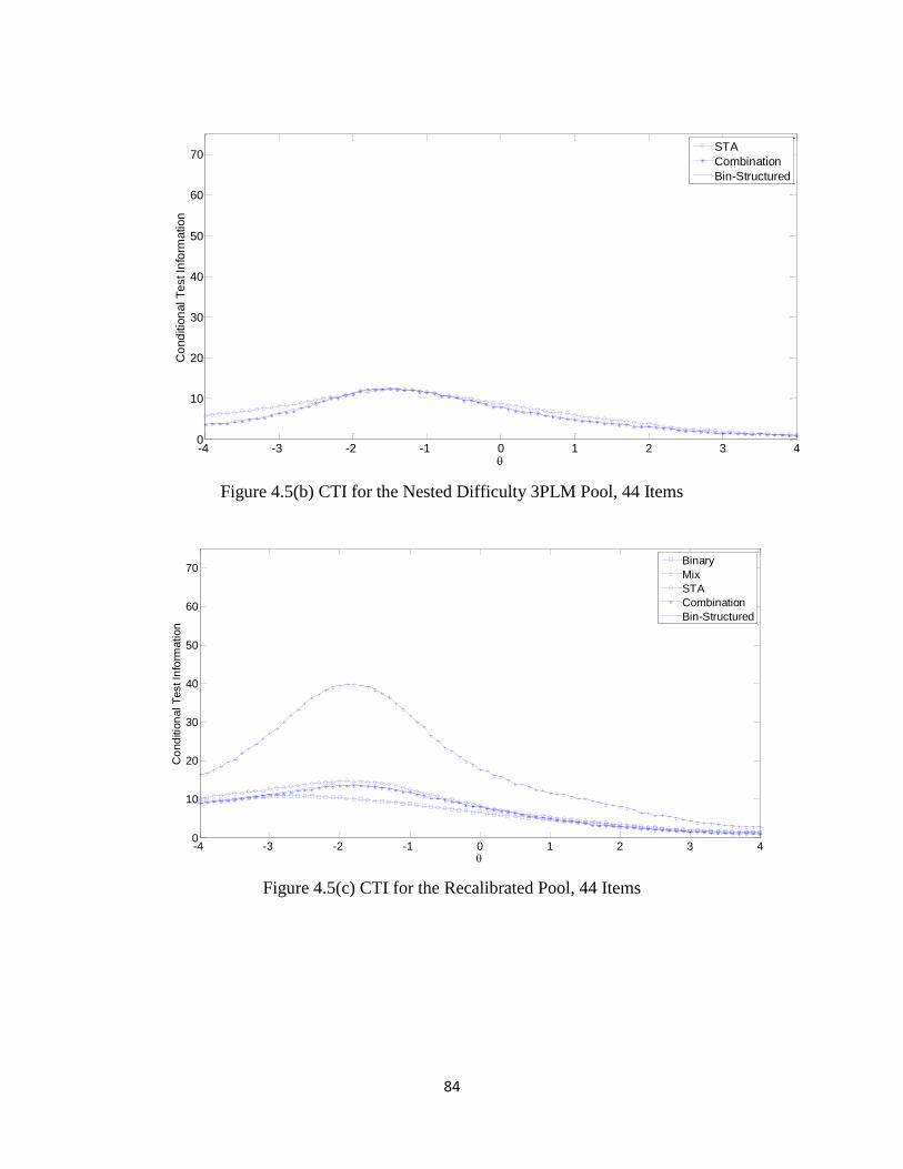
84
Figure 4.5(b) CTI for the Nested Difficulty 3PLM Pool, 44 Items
Figure 4.5(c) CTI for the Recalibrated Pool, 44 Items
-4 -3 -2 -1 0 1 2 3 40
10
20
30
40
50
60
70
Co
nd
itio
nal T
est In
form
ation
STA
Combination
Bin-Structured
-4 -3 -2 -1 0 1 2 3 40
10
20
30
40
50
60
70
Co
nd
itio
nal T
est In
form
ation
Binary
Mix
STA
Combination
Bin-Structured
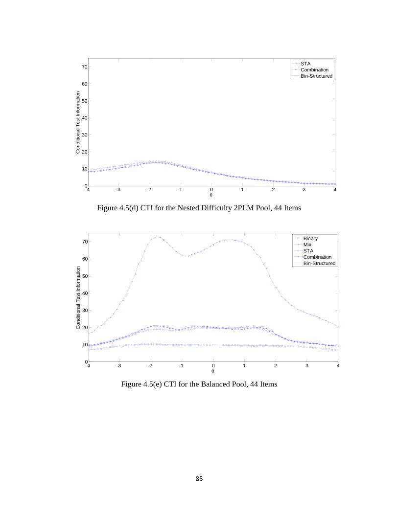
85
Figure 4.5(d) CTI for the Nested Difficulty 2PLM Pool, 44 Items
Figure 4.5(e) CTI for the Balanced Pool, 44 Items
-4 -3 -2 -1 0 1 2 3 40
10
20
30
40
50
60
70
Co
nd
itio
nal T
est In
form
ation
STA
Combination
Bin-Structured
-4 -3 -2 -1 0 1 2 3 40
10
20
30
40
50
60
70
Co
nd
itio
nal T
est In
form
ation
Binary
Mix
STA
Combination
Bin-Structured
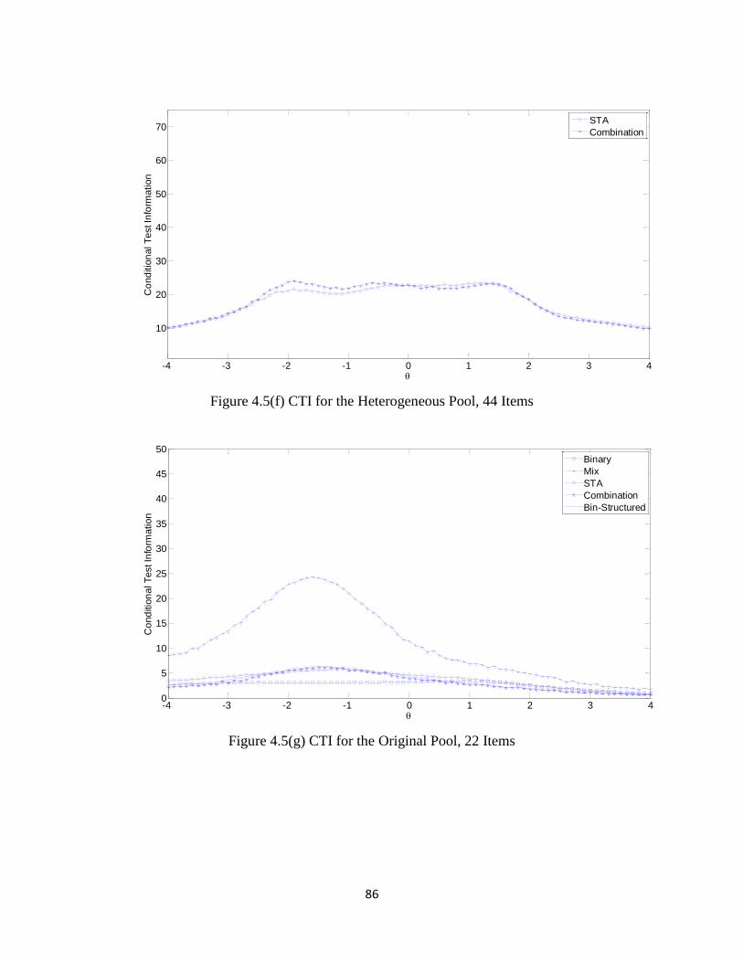
86
Figure 4.5(f) CTI for the Heterogeneous Pool, 44 Items
Figure 4.5(g) CTI for the Original Pool, 22 Items
-4 -3 -2 -1 0 1 2 3 4
10
20
30
40
50
60
70
Co
nd
itio
nal T
est In
form
ation
STA
Combination
-4 -3 -2 -1 0 1 2 3 40
5
10
15
20
25
30
35
40
45
50
Co
nd
itio
nal T
est In
form
ation
Binary
Mix
STA
Combination
Bin-Structured
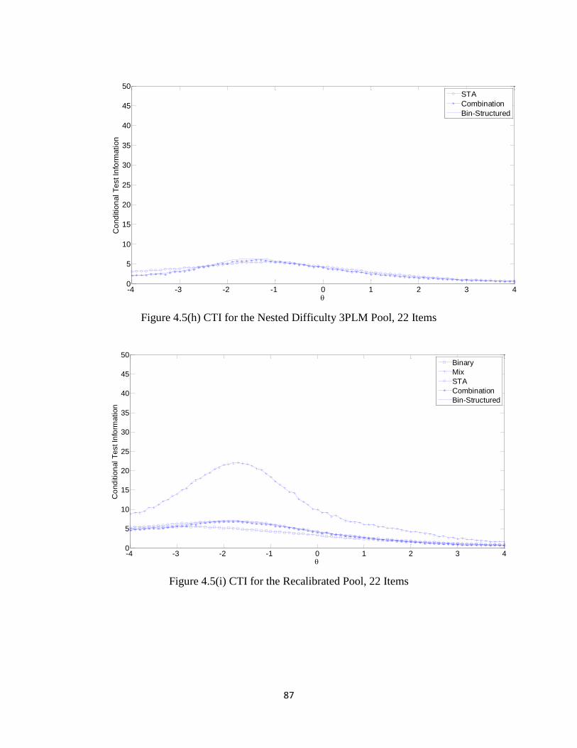
87
Figure 4.5(h) CTI for the Nested Difficulty 3PLM Pool, 22 Items
Figure 4.5(i) CTI for the Recalibrated Pool, 22 Items
-4 -3 -2 -1 0 1 2 3 40
5
10
15
20
25
30
35
40
45
50
Co
nd
itio
nal T
est In
form
ation
STA
Combination
Bin-Structured
-4 -3 -2 -1 0 1 2 3 40
5
10
15
20
25
30
35
40
45
50
Co
nd
itio
nal T
est In
form
ation
Binary
Mix
STA
Combination
Bin-Structured
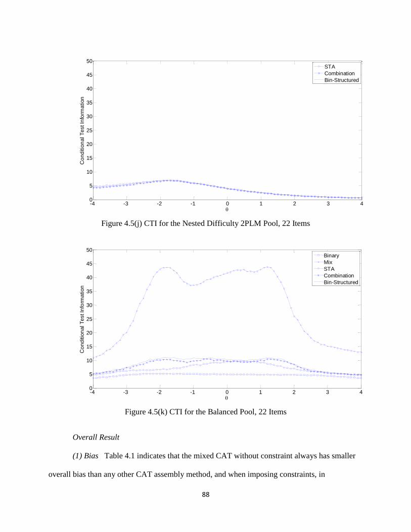
88
Figure 4.5(j) CTI for the Nested Difficulty 2PLM Pool, 22 Items
Figure 4.5(k) CTI for the Balanced Pool, 22 Items
Overall Result
(1) Bias Table 4.1 indicates that the mixed CAT without constraint always has smaller
overall bias than any other CAT assembly method, and when imposing constraints, in
-4 -3 -2 -1 0 1 2 3 40
5
10
15
20
25
30
35
40
45
50
Co
nd
itio
nal T
est In
form
ation
STA
Combination
Bin-Structured
-4 -3 -2 -1 0 1 2 3 40
5
10
15
20
25
30
35
40
45
50
Co
nd
itio
nal T
est In
form
ation
Binary
Mix
STA
Combination
Bin-Structured
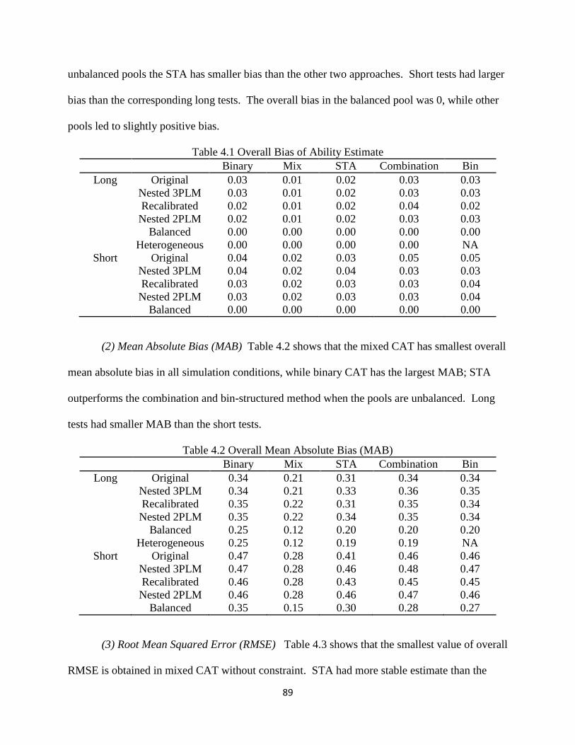
89
unbalanced pools the STA has smaller bias than the other two approaches. Short tests had larger
bias than the corresponding long tests. The overall bias in the balanced pool was 0, while other
pools led to slightly positive bias.
Table 4.1 Overall Bias of Ability Estimate
Binary Mix STA Combination Bin
Long Original 0.03 0.01 0.02 0.03 0.03
Nested 3PLM 0.03 0.01 0.02 0.03 0.03
Recalibrated 0.02 0.01 0.02 0.04 0.02
Nested 2PLM 0.02 0.01 0.02 0.03 0.03
Balanced 0.00 0.00 0.00 0.00 0.00
Heterogeneous 0.00 0.00 0.00 0.00 NA
Short Original 0.04 0.02 0.03 0.05 0.05
Nested 3PLM 0.04 0.02 0.04 0.03 0.03
Recalibrated 0.03 0.02 0.03 0.03 0.04
Nested 2PLM 0.03 0.02 0.03 0.03 0.04
Balanced 0.00 0.00 0.00 0.00 0.00
(2) Mean Absolute Bias (MAB) Table 4.2 shows that the mixed CAT has smallest overall
mean absolute bias in all simulation conditions, while binary CAT has the largest MAB; STA
outperforms the combination and bin-structured method when the pools are unbalanced. Long
tests had smaller MAB than the short tests.
Table 4.2 Overall Mean Absolute Bias (MAB)
Binary Mix STA Combination Bin
Long Original 0.34 0.21 0.31 0.34 0.34
Nested 3PLM 0.34 0.21 0.33 0.36 0.35
Recalibrated 0.35 0.22 0.31 0.35 0.34
Nested 2PLM 0.35 0.22 0.34 0.35 0.34
Balanced 0.25 0.12 0.20 0.20 0.20
Heterogeneous 0.25 0.12 0.19 0.19 NA
Short Original 0.47 0.28 0.41 0.46 0.46
Nested 3PLM 0.47 0.28 0.46 0.48 0.47
Recalibrated 0.46 0.28 0.43 0.45 0.45
Nested 2PLM 0.46 0.28 0.46 0.47 0.46
Balanced 0.35 0.15 0.30 0.28 0.27
(3) Root Mean Squared Error (RMSE) Table 4.3 shows that the smallest value of overall
RMSE is obtained in mixed CAT without constraint. STA had more stable estimate than the
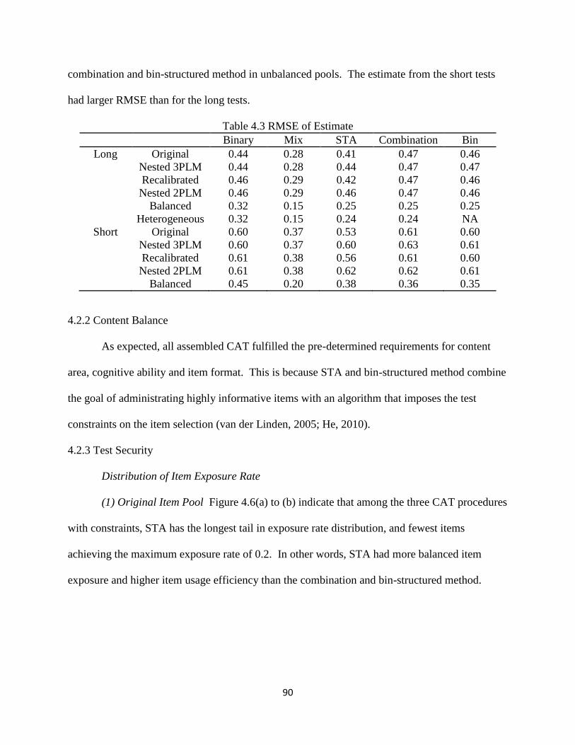
90
combination and bin-structured method in unbalanced pools. The estimate from the short tests
had larger RMSE than for the long tests.
Table 4.3 RMSE of Estimate
Binary Mix STA Combination Bin
Long Original 0.44 0.28 0.41 0.47 0.46
Nested 3PLM 0.44 0.28 0.44 0.47 0.47
Recalibrated 0.46 0.29 0.42 0.47 0.46
Nested 2PLM 0.46 0.29 0.46 0.47 0.46
Balanced 0.32 0.15 0.25 0.25 0.25
Heterogeneous 0.32 0.15 0.24 0.24 NA
Short Original 0.60 0.37 0.53 0.61 0.60
Nested 3PLM 0.60 0.37 0.60 0.63 0.61
Recalibrated 0.61 0.38 0.56 0.61 0.60
Nested 2PLM 0.61 0.38 0.62 0.62 0.61
Balanced 0.45 0.20 0.38 0.36 0.35
4.2.2 Content Balance
As expected, all assembled CAT fulfilled the pre-determined requirements for content
area, cognitive ability and item format. This is because STA and bin-structured method combine
the goal of administrating highly informative items with an algorithm that imposes the test
constraints on the item selection (van der Linden, 2005; He, 2010).
4.2.3 Test Security
Distribution of Item Exposure Rate
(1) Original Item Pool Figure 4.6(a) to (b) indicate that among the three CAT procedures
with constraints, STA has the longest tail in exposure rate distribution, and fewest items
achieving the maximum exposure rate of 0.2. In other words, STA had more balanced item
exposure and higher item usage efficiency than the combination and bin-structured method.
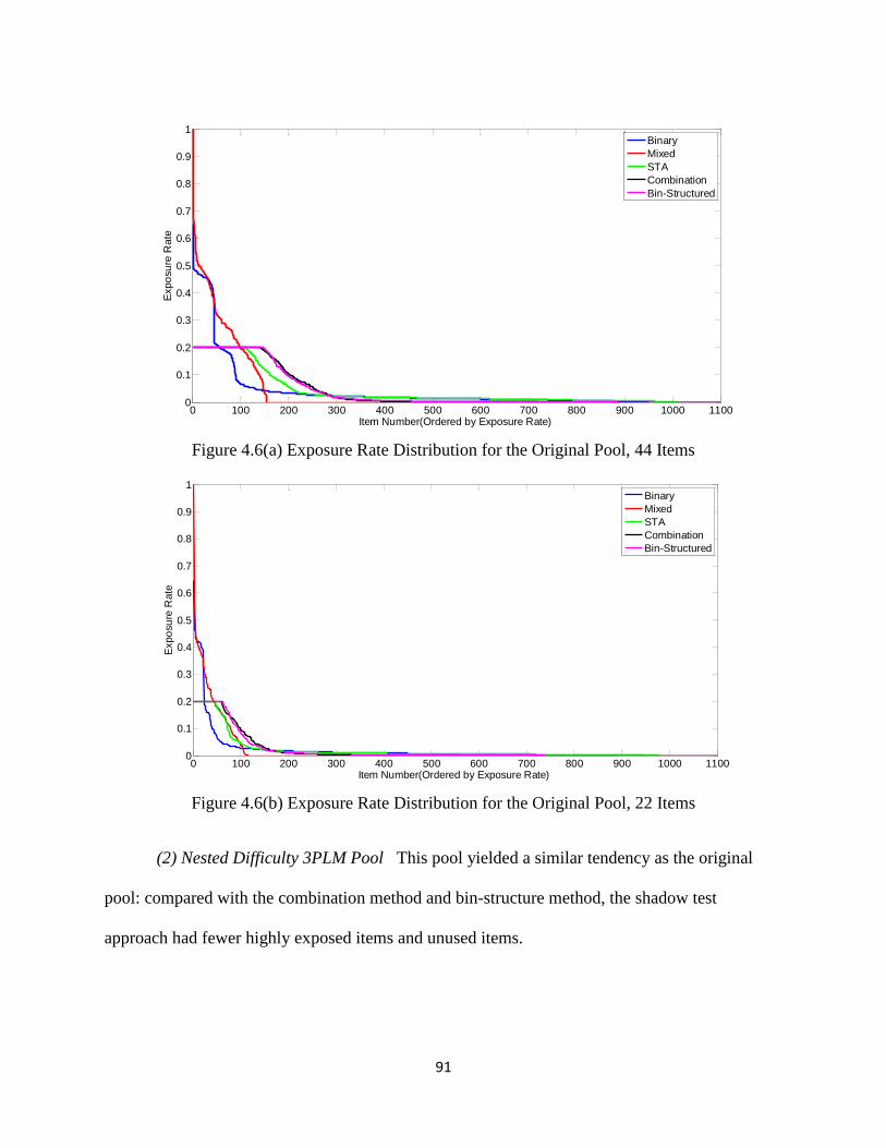
91
Figure 4.6(a) Exposure Rate Distribution for the Original Pool, 44 Items
Figure 4.6(b) Exposure Rate Distribution for the Original Pool, 22 Items
(2) Nested Difficulty 3PLM Pool This pool yielded a similar tendency as the original
pool: compared with the combination method and bin-structure method, the shadow test
approach had fewer highly exposed items and unused items.
0 100 200 300 400 500 600 700 800 900 1000 11000
0.1
0.2
0.3
0.4
0.5
0.6
0.7
0.8
0.9
1
Item Number(Ordered by Exposure Rate)
Expo
su
re R
ate
Binary
Mixed
STA
Combination
Bin-Structured
0 100 200 300 400 500 600 700 800 900 1000 11000
0.1
0.2
0.3
0.4
0.5
0.6
0.7
0.8
0.9
1
Item Number(Ordered by Exposure Rate)
Expo
su
re R
ate
Binary
Mixed
STA
Combination
Bin-Structured
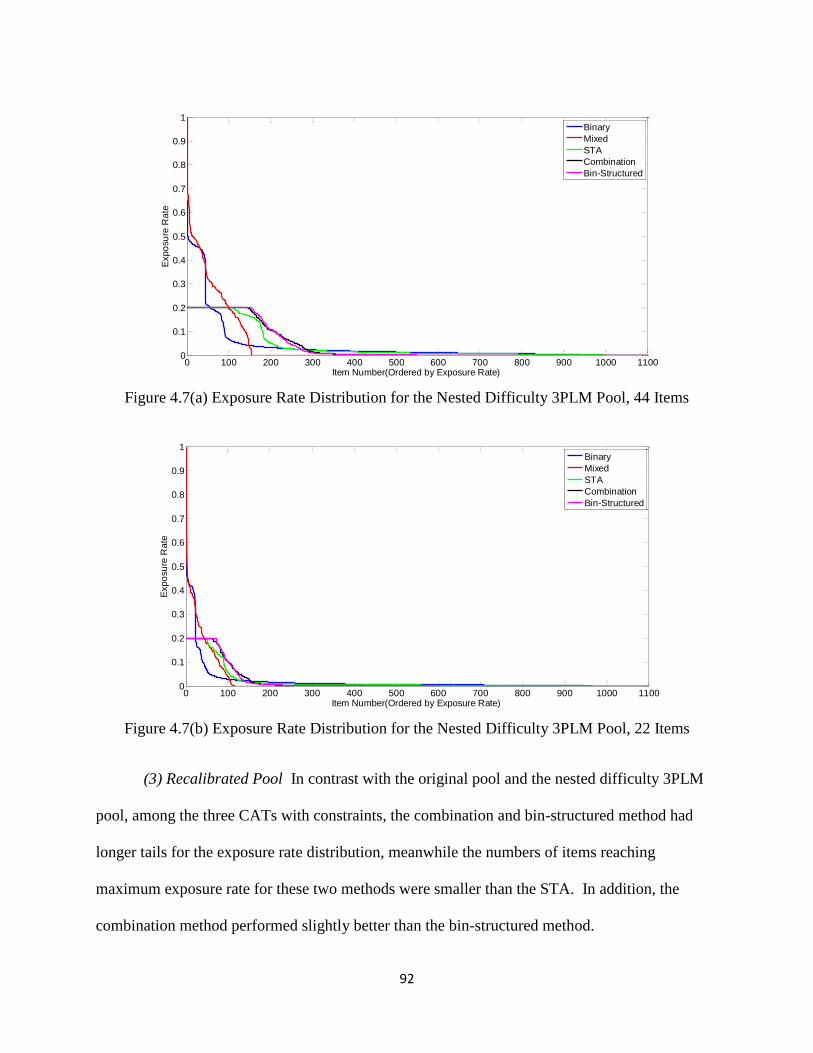
92
Figure 4.7(a) Exposure Rate Distribution for the Nested Difficulty 3PLM Pool, 44 Items
Figure 4.7(b) Exposure Rate Distribution for the Nested Difficulty 3PLM Pool, 22 Items
(3) Recalibrated Pool In contrast with the original pool and the nested difficulty 3PLM
pool, among the three CATs with constraints, the combination and bin-structured method had
longer tails for the exposure rate distribution, meanwhile the numbers of items reaching
maximum exposure rate for these two methods were smaller than the STA. In addition, the
combination method performed slightly better than the bin-structured method.
0 100 200 300 400 500 600 700 800 900 1000 11000
0.1
0.2
0.3
0.4
0.5
0.6
0.7
0.8
0.9
1
Item Number(Ordered by Exposure Rate)
Expo
su
re R
ate
Binary
Mixed
STA
Combination
Bin-Structured
0 100 200 300 400 500 600 700 800 900 1000 11000
0.1
0.2
0.3
0.4
0.5
0.6
0.7
0.8
0.9
1
Item Number(Ordered by Exposure Rate)
Expo
su
re R
ate
Binary
Mixed
STA
Combination
Bin-Structured
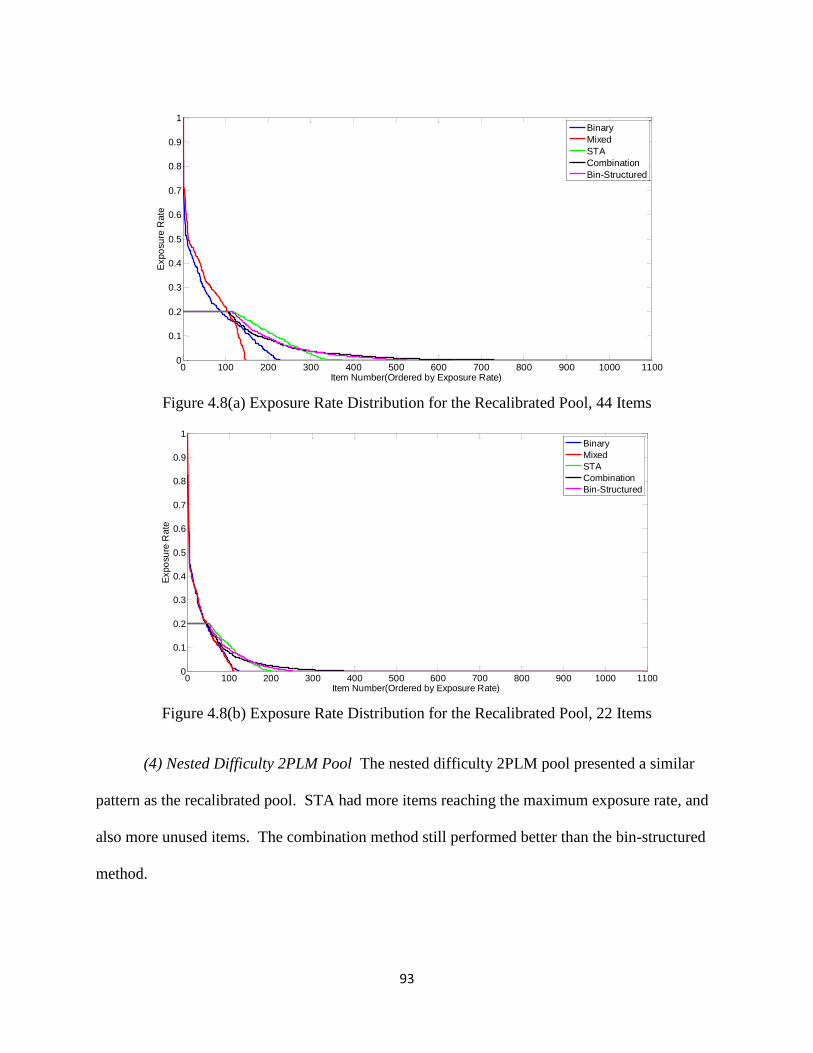
93
Figure 4.8(a) Exposure Rate Distribution for the Recalibrated Pool, 44 Items
Figure 4.8(b) Exposure Rate Distribution for the Recalibrated Pool, 22 Items
(4) Nested Difficulty 2PLM Pool The nested difficulty 2PLM pool presented a similar
pattern as the recalibrated pool. STA had more items reaching the maximum exposure rate, and
also more unused items. The combination method still performed better than the bin-structured
method.
0 100 200 300 400 500 600 700 800 900 1000 11000
0.1
0.2
0.3
0.4
0.5
0.6
0.7
0.8
0.9
1
Item Number(Ordered by Exposure Rate)
Expo
su
re R
ate
Binary
Mixed
STA
Combination
Bin-Structured
0 100 200 300 400 500 600 700 800 900 1000 11000
0.1
0.2
0.3
0.4
0.5
0.6
0.7
0.8
0.9
1
Item Number(Ordered by Exposure Rate)
Expo
su
re R
ate
Binary
Mixed
STA
Combination
Bin-Structured
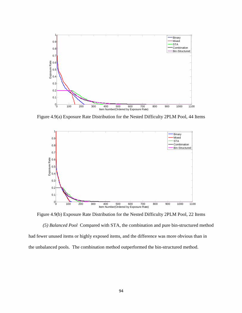
94
Figure 4.9(a) Exposure Rate Distribution for the Nested Difficulty 2PLM Pool, 44 Items
Figure 4.9(b) Exposure Rate Distribution for the Nested Difficulty 2PLM Pool, 22 Items
(5) Balanced Pool Compared with STA, the combination and pure bin-structured method
had fewer unused items or highly exposed items, and the difference was more obvious than in
the unbalanced pools. The combination method outperformed the bin-structured method.
0 100 200 300 400 500 600 700 800 900 1000 11000
0.1
0.2
0.3
0.4
0.5
0.6
0.7
0.8
0.9
1
Item Number(Ordered by Exposure Rate)
Expo
su
re R
ate
Binary
Mixed
STA
Combination
Bin-Structured
0 100 200 300 400 500 600 700 800 900 1000 11000
0.1
0.2
0.3
0.4
0.5
0.6
0.7
0.8
0.9
1
Item Number(Ordered by Exposure Rate)
Expo
su
re R
ate
Binary
Mixed
STA
Combination
Bin-Structured
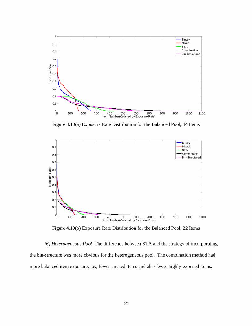
95
Figure 4.10(a) Exposure Rate Distribution for the Balanced Pool, 44 Items
Figure 4.10(b) Exposure Rate Distribution for the Balanced Pool, 22 Items
(6) Heterogeneous Pool The difference between STA and the strategy of incorporating
the bin-structure was more obvious for the heterogeneous pool. The combination method had
more balanced item exposure, i.e., fewer unused items and also fewer highly-exposed items.
0 100 200 300 400 500 600 700 800 900 1000 11000
0.1
0.2
0.3
0.4
0.5
0.6
0.7
0.8
0.9
1
Item Number(Ordered by Exposure Rate)
Expo
su
re R
ate
Binary
Mixed
STA
Combination
Bin-Structured
0 100 200 300 400 500 600 700 800 900 1000 11000
0.1
0.2
0.3
0.4
0.5
0.6
0.7
0.8
0.9
1
Item Number(Ordered by Exposure Rate)
Expo
su
re R
ate
Binary
Mixed
STA
Combination
Bin-Structured
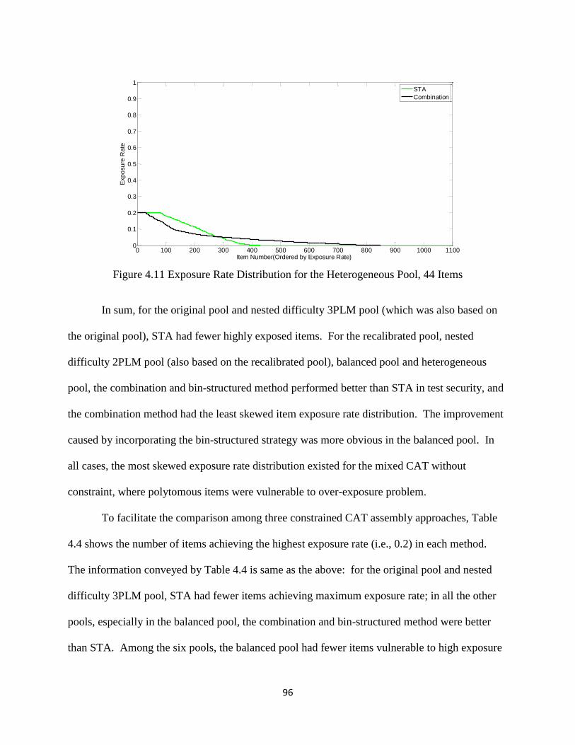
96
Figure 4.11 Exposure Rate Distribution for the Heterogeneous Pool, 44 Items
In sum, for the original pool and nested difficulty 3PLM pool (which was also based on
the original pool), STA had fewer highly exposed items. For the recalibrated pool, nested
difficulty 2PLM pool (also based on the recalibrated pool), balanced pool and heterogeneous
pool, the combination and bin-structured method performed better than STA in test security, and
the combination method had the least skewed item exposure rate distribution. The improvement
caused by incorporating the bin-structured strategy was more obvious in the balanced pool. In
all cases, the most skewed exposure rate distribution existed for the mixed CAT without
constraint, where polytomous items were vulnerable to over-exposure problem.
To facilitate the comparison among three constrained CAT assembly approaches, Table
4.4 shows the number of items achieving the highest exposure rate (i.e., 0.2) in each method.
The information conveyed by Table 4.4 is same as the above: for the original pool and nested
difficulty 3PLM pool, STA had fewer items achieving maximum exposure rate; in all the other
pools, especially in the balanced pool, the combination and bin-structured method were better
than STA. Among the six pools, the balanced pool had fewer items vulnerable to high exposure
0 100 200 300 400 500 600 700 800 900 1000 11000
0.1
0.2
0.3
0.4
0.5
0.6
0.7
0.8
0.9
1
Item Number(Ordered by Exposure Rate)
Expo
su
re R
ate
STA
Combination
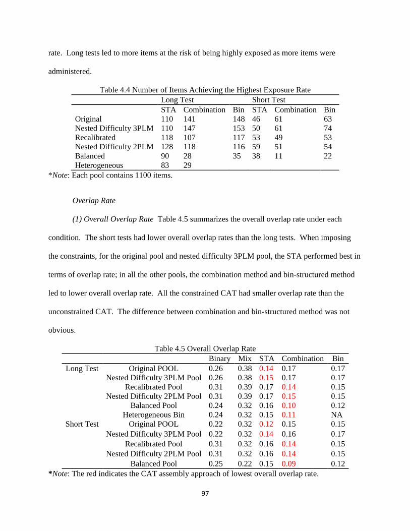
97
rate. Long tests led to more items at the risk of being highly exposed as more items were
administered.
Table 4.4 Number of Items Achieving the Highest Exposure Rate
Long Test Short Test
STA Combination Bin STA Combination Bin
Original 110 141 148 46 61 63
Nested Difficulty 3PLM 110 147 153 50 61 74
Recalibrated 118 107 117 53 49 53
Nested Difficulty 2PLM 128 118 116 59 51 54
Balanced 90 28 35 38 11 22
Heterogeneous 83 29
*Note: Each pool contains 1100 items.
Overlap Rate
(1) Overall Overlap Rate Table 4.5 summarizes the overall overlap rate under each
condition. The short tests had lower overall overlap rates than the long tests. When imposing
the constraints, for the original pool and nested difficulty 3PLM pool, the STA performed best in
terms of overlap rate; in all the other pools, the combination method and bin-structured method
led to lower overall overlap rate. All the constrained CAT had smaller overlap rate than the
unconstrained CAT. The difference between combination and bin-structured method was not
obvious.
Table 4.5 Overall Overlap Rate
Binary Mix STA Combination Bin
Long Test Original POOL 0.26 0.38 0.14 0.17 0.17
Nested Difficulty 3PLM Pool 0.26 0.38 0.15 0.17 0.17
Recalibrated Pool 0.31 0.39 0.17 0.14 0.15
Nested Difficulty 2PLM Pool 0.31 0.39 0.17 0.15 0.15
Balanced Pool 0.24 0.32 0.16 0.10 0.12
Heterogeneous Bin 0.24 0.32 0.15 0.11 NA
Short Test Original POOL 0.22 0.32 0.12 0.15 0.15
Nested Difficulty 3PLM Pool 0.22 0.32 0.14 0.16 0.17
Recalibrated Pool 0.31 0.32 0.16 0.14 0.15
Nested Difficulty 2PLM Pool 0.31 0.32 0.16 0.14 0.15
Balanced Pool 0.25 0.22 0.15 0.09 0.12
*Note: The red indicates the CAT assembly approach of lowest overall overlap rate.
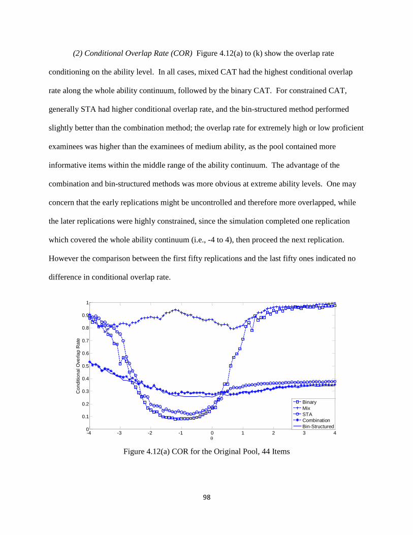
98
(2) Conditional Overlap Rate (COR) Figure 4.12(a) to (k) show the overlap rate
conditioning on the ability level. In all cases, mixed CAT had the highest conditional overlap
rate along the whole ability continuum, followed by the binary CAT. For constrained CAT,
generally STA had higher conditional overlap rate, and the bin-structured method performed
slightly better than the combination method; the overlap rate for extremely high or low proficient
examinees was higher than the examinees of medium ability, as the pool contained more
informative items within the middle range of the ability continuum. The advantage of the
combination and bin-structured methods was more obvious at extreme ability levels. One may
concern that the early replications might be uncontrolled and therefore more overlapped, while
the later replications were highly constrained, since the simulation completed one replication
which covered the whole ability continuum (i.e., -4 to 4), then proceed the next replication.
However the comparison between the first fifty replications and the last fifty ones indicated no
difference in conditional overlap rate.
Figure 4.12(a) COR for the Original Pool, 44 Items
-4 -3 -2 -1 0 1 2 3 40
0.1
0.2
0.3
0.4
0.5
0.6
0.7
0.8
0.9
1
Co
nd
itio
nal O
ve
rla
p R
ate
Binary
Mix
STA
Combination
Bin-Structured
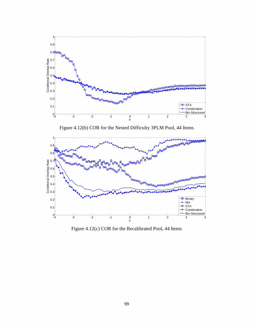
99
Figure 4.12(b) COR for the Nested Difficulty 3PLM Pool, 44 Items
Figure 4.12(c) COR for the Recalibrated Pool, 44 Items
-4 -3 -2 -1 0 1 2 3 40
0.1
0.2
0.3
0.4
0.5
0.6
0.7
0.8
0.9
1
Co
nd
itio
nal O
ve
rla
p R
ate
STA
Combination
Bin-Structured
-4 -3 -2 -1 0 1 2 3 40
0.1
0.2
0.3
0.4
0.5
0.6
0.7
0.8
0.9
1
Co
nd
itio
nal O
ve
rla
p R
ate
Binary
Mix
STA
Combination
Bin-Structured
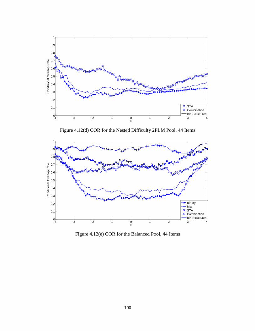
100
Figure 4.12(d) COR for the Nested Difficulty 2PLM Pool, 44 Items
Figure 4.12(e) COR for the Balanced Pool, 44 Items
-4 -3 -2 -1 0 1 2 3 40
0.1
0.2
0.3
0.4
0.5
0.6
0.7
0.8
0.9
1
Co
nd
itio
nal O
ve
rla
p R
ate
STA
Combination
Bin-Structured
-4 -3 -2 -1 0 1 2 3 40
0.1
0.2
0.3
0.4
0.5
0.6
0.7
0.8
0.9
1
Co
nd
itio
nal O
ve
rla
p R
ate
Binary
Mix
STA
Combination
Bin-Structured
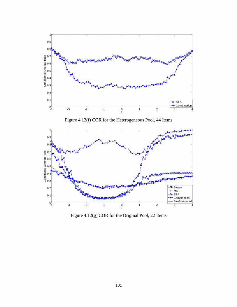
101
Figure 4.12(f) COR for the Heterogeneous Pool, 44 Items
Figure 4.12(g) COR for the Original Pool, 22 Items
-4 -3 -2 -1 0 1 2 3 40
0.1
0.2
0.3
0.4
0.5
0.6
0.7
0.8
0.9
1
Co
nd
itio
nal O
ve
rla
p R
ate
STA
Combination
-4 -3 -2 -1 0 1 2 3 40
0.1
0.2
0.3
0.4
0.5
0.6
0.7
0.8
0.9
1
Co
nd
itio
nal O
ve
rla
p R
ate
Binary
Mix
STA
Combination
Bin-Structured
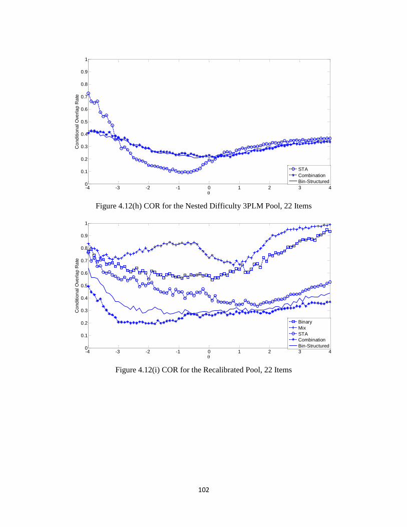
102
Figure 4.12(h) COR for the Nested Difficulty 3PLM Pool, 22 Items
Figure 4.12(i) COR for the Recalibrated Pool, 22 Items
-4 -3 -2 -1 0 1 2 3 40
0.1
0.2
0.3
0.4
0.5
0.6
0.7
0.8
0.9
1
Co
nd
itio
nal O
ve
rla
p R
ate
STA
Combination
Bin-Structured
-4 -3 -2 -1 0 1 2 3 40
0.1
0.2
0.3
0.4
0.5
0.6
0.7
0.8
0.9
1
Co
nd
itio
nal O
ve
rla
p R
ate
Binary
Mix
STA
Combination
Bin-Structured
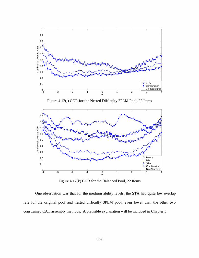
103
Figure 4.12(j) COR for the Nested Difficulty 2PLM Pool, 22 Items
Figure 4.12(k) COR for the Balanced Pool, 22 Items
One observation was that for the medium ability levels, the STA had quite low overlap
rate for the original pool and nested difficulty 3PLM pool, even lower than the other two
constrained CAT assembly methods. A plausible explanation will be included in Chapter 5.
-4 -3 -2 -1 0 1 2 3 40
0.1
0.2
0.3
0.4
0.5
0.6
0.7
0.8
0.9
1
Co
nd
itio
nal O
ve
rla
p R
ate
STA
Combination
Bin-Structured
-4 -3 -2 -1 0 1 2 3 40
0.1
0.2
0.3
0.4
0.5
0.6
0.7
0.8
0.9
1
Co
nd
itio
nal O
ve
rla
p R
ate
Binary
Mix
STA
Combination
Bin-Structured
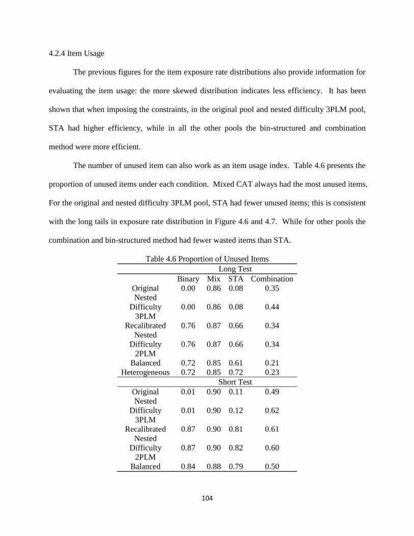
104
4.2.4 Item Usage
The previous figures for the item exposure rate distributions also provide information for
evaluating the item usage: the more skewed distribution indicates less efficiency. It has been
shown that when imposing the constraints, in the original pool and nested difficulty 3PLM pool,
STA had higher efficiency, while in all the other pools the bin-structured and combination
method were more efficient.
The number of unused item can also work as an item usage index. Table 4.6 presents the
proportion of unused items under each condition. Mixed CAT always had the most unused items.
For the original and nested difficulty 3PLM pool, STA had fewer unused items; this is consistent
with the long tails in exposure rate distribution in Figure 4.6 and 4.7. While for other pools the
combination and bin-structured method had fewer wasted items than STA.
Table 4.6 Proportion of Unused Items
Long Test
Binary Mix STA Combination
Original 0.00 0.86 0.08 0.35
Nested
Difficulty
3PLM
0.00 0.86 0.08 0.44
Recalibrated 0.76 0.87 0.66 0.34
Nested
Difficulty
2PLM
0.76 0.87 0.66 0.34
Balanced 0.72 0.85 0.61 0.21
Heterogeneous 0.72 0.85 0.72 0.23
Short Test
Original 0.01 0.90 0.11 0.49
Nested
Difficulty
3PLM
0.01 0.90 0.12 0.62
Recalibrated 0.87 0.90 0.81 0.61
Nested
Difficulty
2PLM
0.87 0.90 0.82 0.60
Balanced 0.84 0.88 0.79 0.50
105
Chapter 5: Summary and Discussion
This chapter contains a summary and a discussion. To start with, the research objectives,
methodology used in this study, and results are summarized. The second section has the
discussion of the major findings. The last part discusses the implications and limitations of this
study, and also provides suggestions for future research.
5.1 Summary of This Study
The main purposes of this study were (1) to investigate whether the mixed-item-based
CAT had advantages over the dichotomous-item-based CAT and what challenges it brought; (2)
to compare the STA with the bin-structured method in mixed-item CAT assembly, and to
explore what were some factors that might influence the assembly effect. A simulation study
was conducted to compare five CAT test assembly approaches (i.e., binary CAT, mixed CAT,
STA, combination of STA and bin-structured method, and bin-structured method) in a variety of
testing situations specifying the test objectives and constraints. The goal of the simulated CAT
was to construct efficient, content (including content areas, item format and cognitive skills)
balanced and secure tests. The effectiveness of assembly was evaluated through four types of
criteria, including measurement, content balance, test security and item usage. The shape of item
pool, test length, and imposed constraints were manipulated to explore how the findings varied.
5.1.1 Measurement Criteria
No difference in conditional bias of ability estimate among the five CAT assembly
methods was found. The ability was overestimated at the lower end of ability continuum, and
underestimated at the upper end; the magnitude for underestimation was larger. This trend was
more obvious when the unbalanced pool was used, as the pool contained fewer informative items
106
for measuring the high ability levels. Conditional on ability level, short tests had larger bias than
the long tests.
Along the entire ability continuum, the mixed CAT always had smallest absolute bias and
SEM among the five CAT assembly approaches. The absolute bias and SEM for high-
proficiency examinees was larger than the examinees at other ability levels. The three
constrained CAT assembly approaches had similar results. When the pool was balanced, all the
four approaches involving polytomous items had smaller absolute bias and SEM than the binary
CAT. When the pool was unbalanced, within the relatively low ability range, CAT incorporating
polytomous items performed better than the unconstrained binary CAT even when constraints
were imposed to the mixed CAT, as the pool contained many informative items in this range.
Shorter tests had larger absolute bias and SEM than long tests given the ability level. The
information from TCSEM also reinforced these findings.
In terms of overall measurement issues, the mixed CAT worked best. STA had smaller
bias, MAB and RMSE than the combination and bin-structured method in unbalanced pools.
5.1.2 Content Balance
All the simulations satisfied the content balance requirements.
5.1.3 Item Exposure Rate Distribution
In sum, with the original pool and nested difficulty 3PLM pool (also based on the original
pool), STA had fewer high-exposure items and lower overall overlap rate. For the recalibrated
pool, nested difficulty 2PLM pool (also based on the recalibrated pool), balanced pool and
heterogeneous pool, the combination and pure bin-structured method performed better than STA
in test security, and the combination method had least skewed item exposure rate distribution.
The improvement caused by incorporating bin-structured strategy was more obvious in the
107
balanced pool. In all cases, the most skewed exposure rate distribution and highest overlap rate
existed in the mixed CAT without constraint, where polytomous items were vulnerable to over-
exposure.
Conditioning on ability level, generally STA had higher conditional overlap rate, and the
bin-structured method performed slightly better than the combination method; the overlap rate
for extremely high or low ability examinees was higher than the examinees of medium ability, as
the pool contained more informative items within the middle range of the ability continuum. The
advantage of the combination and bin-structured method was more obvious at extreme ability
levels.
5.1.4 Item Usage
The efficiency of item usage was lowest in mixed CAT. When imposing the constraints,
in the original pool and nested difficulty 3PLM pool, STA had higher efficiency, while in all the
other pools the bin-structured and combination method were more efficient.
5.2 Discussion of Major Findings
5.2.1 Incorporating Polytomous Items into CAT
As stated before, polytomous items are receiving growing attention in CAT, as it can
evaluate an examinee's partial knowledge, assess high-level cognitive skills, and improve the test
validity. The development of polytomous response models and progress in computer
computation allow for future flourishing application of polytomous items in CAT, and expanding
the use of polytomous items in CAT is already on the agenda. This study confirmed the
contribution of polytomous items to building an effective CAT, as in all conditions the mixed
CAT led to smaller bias, absolute bias, and SEM than other CAT assembly methods. However
one consequent problem is over-exposure of the polytomous items, as the highly informative
108
items are tend to be more frequently selected. This problem was also verified in this study: the
mixed CAT had the most skewed exposure rate distribution, and further analysis showed that the
highly exposed items were all polytomous items. Considering the tedious work of developing
the polytomous items, how to protect them from severe security problems was a critical issue.
One related problem for mixed CAT was its low item usage efficiency, as a lot of items (mainly
dichotomous items) were unused.
When adding constraints to CAT assembly, especially the rules to control the exposure
rate, the CAT efficiency would be compromised as maximum information was no longer the
unique criterion for selecting items; this was reflected by the increasing bias and SEM. This
influence might be aggravated if the psychometric properties of items were entangled with the
categorical attribute specified in the blueprint, e.g., content area. This was why the nested
difficulty 3PLM pool performed worse than the original pool (i.e., had larger MAB and RMSE),
and nested difficulty 2PLM pool was worse than the recalibrated pool. The requirement for
content balance forced the examinees to take less informative items, and therefore the efficiency
of CAT was reduced. However the constraints may balance the item usage: fewer items were
suffering from high-exposure. This study only set an upper bound for exposure rate, but a lower
bound could also be set to reduce the underused items. Appropriate boundary value should be
determined to guarantee that the pool has reasonable item usage while the assembled CAT can
still estimate the ability efficiently.
5.2.2 Comparing STA and Bin-Structured Method
Both STA and bin-structured method have the same goal for test construction: optimize a
test’s measurement efficiency and ensure the test can satisfy all the test specifications. But they
proceed in different ways. The STA finds a unique and optimal solution for every examinee; this
109
can effectively construct highly informative test, but the cost is also high. Because searching for
the best solution is conducted in the entire pool, the computation in STA may be formidable. On
the other hand, the bin-structured approach partitions the item bank into non-overlapping item
sets so that each item selection step is completed within a bin, which greatly simplifies the item
selection procedures.
Besides reducing the calculation burden, the bin-structured method also has other
advantages. By dividing the items into bins in accordance with the pre-specified test length and
specifications, the bin-structured method automatically produces content valid tests. This
template takes care of the feasibility issues that most item selection algorithms have to face to,
and also can be reviewed in advance to enhance the test validity (Robin, 2005). Furthermore, as
the bin-structured method adopts a unique template for all examinees, tests across examinees will
be more similar to each other; the examinees are less likely to be disturbed by unexpected item
topic or format sequences (Davey, 2005), and the context effect will be diminished. By
eliminating the factors irrelevant to the target trait but influencing the performance, the bin-
structured method makes the tests more comparable across the examinees.
Bin-structure can also help to improve the item usage. In this study, the bin-structured
method had a lower conditional overlap rate than STA, especially for examinees of extremely
high or low ability; and it also had more balanced item exposure rate distribution in most of the
pools, with the only exception in the original pool and nested difficulty 3PLM pool. An
explanation for this result will be provided later. In addition, as the item selection was conducted
in each bin, the item replacement and exposure control would be easier in bin-structured method.
One intuition is that the bin-structured method may construct less informative tests than
STA, as the STA selects the next item in the entire pool and is less restricted. However this
110
study showed this was not necessarily the case: the bin-structure method had comparable
conditional bias and SEM to STA. The reason was that when developing the bins, the later bins
contained more informative items, which improved the effectiveness of bin-structured method.
This emphasized the importance of producing and organizing bins properly. An example (see
Table 5.1) on item usage in bin-structured method would be given later to underline the
significance of producing proper bins.
5.2.3 Developing Bins Properly
Whether the bin-structured method performs well depends on the quality of bins.
Whether the bins can be divided efficiently is influenced by the characteristics of the item pool.
For instance, in this study, in most cases, the bin-structured method can assemble equally good
or even better CATs than STA. One exception was that in the original and nested difficulty
3PLM pool, STA had slightly smaller TCSEM than the combination and bin-structured method,
especially at the extreme ability levels. This was due to the fact that the item pools had fewer
informative items for examinees within this ability range and the quality of developed bins
would be compromised, while the STA had more options as it searched for the optimum item in
the whole pool.
An example may help focus in on the influence of item pool on the bin-structured method.
Table 5.1 compares the combination method in nested difficulty 3PLM pool and balanced pool.
When dividing the items in nested difficulty 3PLM pool into bins, the distance between b-
parameter and 0 was used as the criterion: items in early bins were closer to 0, and in later bins
were further from 0. However as the pool contains more easy items than hard items, the later
bins may have a large proportion of items with low b-parameter and only a few items appropriate
for measuring high-proficiency examinees. Therefore as shown in Table 5.1, in the nested
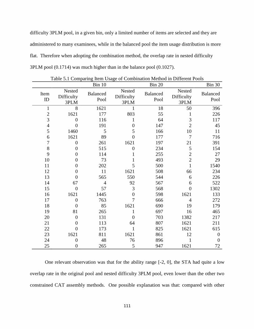
111
difficulty 3PLM pool, in a given bin, only a limited number of items are selected and they are
administered to many examinees, while in the balanced pool the item usage distribution is more
flat. Therefore when adopting the combination method, the overlap rate in nested difficulty
3PLM pool (0.1714) was much higher than in the balance pool (0.1027).
Table 5.1 Comparing Item Usage of Combination Method in Different Pools
Bin 10 Bin 20 Bin 30
Item
ID
Nested
Difficulty
3PLM
Balanced
Pool
Nested
Difficulty
3PLM
Balanced
Pool
Nested
Difficulty
3PLM
Balanced
Pool
1 8 1621 1 18 50 396
2 1621 177 803 55 1 226
3 0 116 1 64 3 117
4 0 191 0 147 2 45
5 1460 5 5 166 10 11
6 1621 89 0 177 7 716
7 0 261 1621 197 21 391
8 0 515 0 234 5 154
9 0 114 1 255 2 27
10 0 73 1 493 2 29
11 0 202 5 500 1 1540
12 0 11 1621 508 66 234
13 0 565 550 544 6 226
14 67 4 92 567 6 522
15 0 57 3 568 0 1302
16 1621 1445 0 598 1621 133
17 0 763 7 666 4 272
18 0 85 1621 690 19 179
19 81 265 1 697 16 465
20 0 131 0 703 1382 217
21 0 113 64 807 1621 211
22 0 173 1 825 1621 615
23 1621 811 1621 861 12 0
24 0 48 76 896 1 0
25 0 265 5 947 1621 72
One relevant observation was that for the ability range [-2, 0], the STA had quite a low
overlap rate in the original pool and nested difficulty 3PLM pool, even lower than the other two
constrained CAT assembly methods. One possible explanation was that: compared with other
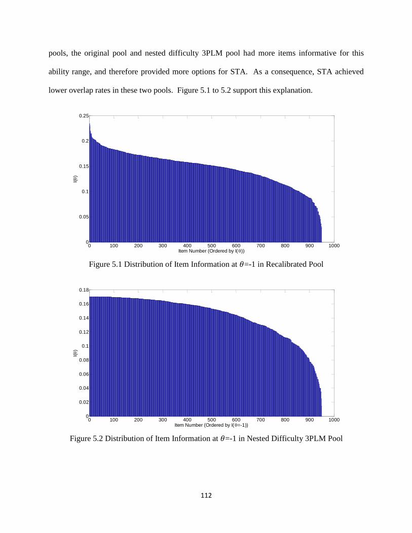
112
pools, the original pool and nested difficulty 3PLM pool had more items informative for this
ability range, and therefore provided more options for STA. As a consequence, STA achieved
lower overlap rates in these two pools. Figure 5.1 to 5.2 support this explanation.
Figure 5.1 Distribution of Item Information at =-1 in Recalibrated Pool
Figure 5.2 Distribution of Item Information at =-1 in Nested Difficulty 3PLM Pool
0 100 200 300 400 500 600 700 800 900 10000
0.05
0.1
0.15
0.2
0.25
Item Number (Ordered by I())
I()
0 100 200 300 400 500 600 700 800 900 10000
0.02
0.04
0.06
0.08
0.1
0.12
0.14
0.16
0.18
Item Number (Ordered by I(=-1))
I()
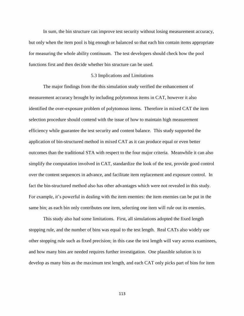
113
In sum, the bin structure can improve test security without losing measurement accuracy,
but only when the item pool is big enough or balanced so that each bin contain items appropriate
for measuring the whole ability continuum. The test developers should check how the pool
functions first and then decide whether bin structure can be used.
5.3 Implications and Limitations
The major findings from the this simulation study verified the enhancement of
measurement accuracy brought by including polytomous items in CAT, however it also
identified the over-exposure problem of polytomous items. Therefore in mixed CAT the item
selection procedure should contend with the issue of how to maintain high measurement
efficiency while guarantee the test security and content balance. This study supported the
application of bin-structured method in mixed CAT as it can produce equal or even better
outcomes than the traditional STA with respect to the four major criteria. Meanwhile it can also
simplify the computation involved in CAT, standardize the look of the test, provide good control
over the content sequences in advance, and facilitate item replacement and exposure control. In
fact the bin-structured method also has other advantages which were not revealed in this study.
For example, it’s powerful in dealing with the item enemies: the item enemies can be put in the
same bin; as each bin only contributes one item, selecting one item will rule out its enemies.
This study also had some limitations. First, all simulations adopted the fixed length
stopping rule, and the number of bins was equal to the test length. Real CATs also widely use
other stopping rule such as fixed precision; in this case the test length will vary across examinees,
and how many bins are needed requires further investigation. One plausible solution is to
develop as many bins as the maximum test length, and each CAT only picks part of bins for item
114
selection. But the test developers should organize the sequence of bins carefully so that each
administration can satisfy the requirement for content balance.
Second, this study set fixed proportions for each content area. Further research can set
upper and lower bounds for content balance requirements, for example, the CAT might require
that at least 10% of the items are polytomous. This change will bring difficulty to bin
development, as the number of bins in each content area is not determined. Again, one possible
solution is to make the number of bins of a certain type equal to the upper bound of the
requirement for this category.
Third, only one template was used in this study. Operational CAT can develop multiple
templates to further reduce overlap rate and improve item usage. The number of required
templates depends on the characteristics of the item pool and the tested population. Future study
can investigate how to develop parallel templates efficiently.
Fourth, the number of items in different bins kept the same in this study. Future research
can vary the bin size in different CAT stages. For example, the later bins may contain more
items than the early bins since the later bins are expected to provide accurate measurement along
a wider ability range. Following research can also investigate what the minimum number of item
in each bin is.
Fifth, the original OSSLT was designed for a single cut-score and following analysis may
focus the results around the cut-score, and investigate the influence of the cut-score. Another
potential research direction is to use bin-structure in computerized classification testing, where
the goal is to classify examinees in an adaptive way.

115
At last, the simulation set even-space distribution for the examinee ability, which may
overweigh the tails of the distribution. Future research may set normal or empirical distribution,
or attach different weight to see how the results vary.
In sum, this study supported the application of polytomous items in CAT, as they can
enhance test validity, as well as measurement accuracy and stability. However it also showed
that the polytomous items were more vulnerable to over-exposure. Both STA and bin-structured
method could help to control item exposure rate in mixed-item-based CAT; meanwhile, they
could satisfy all the test requirements. When the item pool was not severely skewed and bins can
be developed properly, the bin-structured method was recommended.

116
BIBLIOGRAPHY
117
BIBLIOGRAPHY
Akkermans, W., & Muraki, E. (1997). Item information and discrimination functions for trinary
PCM items. Psychometrika, 62(4), 569-578.
Ahmed, A., Pollitt, A., Crisp, V., & Sweiry, E. (2003). Writing examinations questions.
Attali, Y., & Burstein, J. (2006). Automated essay scoring with e-rater® V. 2. The
Journal of Technology, Learning and Assessment, 4(3).
Bergstrom, B. A., & Lunz, M. E. (1999). CAT for certification and licensure. Innovations
in computerized assessment, 67-91.
Binet, A., & Simon, T. (1905). New methods for the diagnosis of the intellectual level of
subnormals. L’annee Psychologique, 12, 191-244.
Birnbaum, A. (1968). Some latent train models and their use in inferring an examinee's
ability. Statistical theories of mental test scores, 395-479.
Bock, R. D. (1972). Estimating item parameters and latent ability when responses are scored in
two or more nominal categories. Psychometrika, 37(1), 29-51.
Bock, R. D., & Aitkin, M. (1981). Marginal maximum likelihood estimation of item parameters:
Application of an EM algorithm. Psychometrika, 46(4), 443-459.
Burton, R. F. (2001). Quantifying the effects of chance in multiple choice and true/false tests:
question selection and guessing of answers. Assessment & Evaluation in Higher
Education, 26(1), 41-50.
Cai, L. (2012). flexMIRT: Flexible multilevel item factor analysis and test scoring [Computer
software]. Seattle, WA: Vector Psychometric Group, LLC.
Cao, Y. (2008). Mixed-format test equating: Effects of test dimensionality and common-item sets.
ProQuest.
Chang, H. (2004). Understanding Computerized Adaptive Testing. The SAGE handbook of
quantitative methodology for the social sciences, 117.
Chang, H. H., Qian, J., & Ying, Z. (2001). a-Stratified multistage computerized adaptive testing
with b blocking. Applied Psychological Measurement, 25(4), 333-341.
Chang, H. H., & Ying, Z. (1996). A global information approach to computerized adaptive
testing. Applied Psychological Measurement, 20(3), 213-229.
118
Chang, H. H., & Ying, Z. (1999). A-stratified multistage computerized adaptive testing. Applied
Psychological Measurement, 23(3), 211-222.
Chen, S. Y., & Ankenman, R. D. (2004). Effects of practical constraints on item selection rules
at the early stages of computerized adaptive testing.Journal of Educational
Measurement, 41(2), 149-174.
Chen, S. K., Hou, L., & Dodd, B. G. (1998). A comparison of maximum likelihood estimation
and expected a posteriori estimation in CAT using the partial credit model. Educational
and Psychological Measurement, 58(4), 569-595.
Chen, S. K., Hou, L., Fitzpatrick, S. J., & Dodd, B. G. (1997). The effect of population
distribution and method of theta estimation on computerized adaptive testing (CAT)
using the rating scale model. Educational and psychological measurement, 57(3), 422-
439.
Cheng, Y., & Chang, H. H. (2009). The maximum priority index method for severely
constrained item selection in computerized adaptive testing. British Journal of
Mathematical and Statistical Psychology, 62(2), 369-383.
Choi, S. W., & Swartz, R. J. (2009). Comparison of CAT item selection criteria for polytomous
items. Applied Psychological Measurement.
Cook, K. F., Dodd, B. G., & Fitzpatrick, S. J. (1998). A comparison of three polytomous item
response theory models in the context of testlet scoring. Journal of outcome measurement,
3(1), 1-20.
Davey, T. (2005, April). An Introduction to bin-structured Adaptive Testing. Presented at the
annual meeting of the American Educational Research Association, Montreal.
Davey, T., & Parshall, C. G. (1995). New Algorithms for Item Selection and Exposure Control
with Computerized Adaptive Testing.
Davis, L. L. (2004). Strategies for controlling item exposure in computerized adaptive testing
with the generalized partial credit model. Applied Psychological Measurement, 28(3),
165-185.
Dodd, B. G., & Koch, W. R. (1987). Effects of variations in item step values on item and test
information in the partial credit model. Applied Psychological Measurement, 11(4), 371-
384.
Drasgow, F., Levine, M. V., Williams, B., McLaughlin, M. E., & Candell, G. L. (1989).
Modeling incorrect responses to multiple-choice items with multilinear formula score
theory. Applied Psychological Measurement, 13(3), 285-299.
119
Enright, M. K., Morley, M., & Sheehan, K. M. (2002). Items by design: The impact of
systematic feature variation on item statistical characteristics.Applied Measurement in
Education, 15(1), 49-74.
Glas, C. A., & van der Linden, W. J. (2003). Computerized adaptive testing with item
cloning. Applied Psychological Measurement, 27(4), 247-261.
Green, B. F., Bock, R. D., Humphreys, L. G., Linn, R. L., & Reckase, M. D. (1984). Technical
guidelines for assessing computerized adaptive tests.Journal of Educational
Measurement, 21(4), 347-360.
Gu, L. (2007). Designing optimal item pools for computerized adaptive tests with exposure
controls. Unpublished doctoral dissertation. Michigan State University.
Haladyna, T. M. (1994). A research agenda for licensing and certification testing validation
studies. Evaluation & the health professions, 17(2), 242-256.
Hambleton, R. K., & Swaminathan, H. (1985). Item response theory: Principles and
applications (Vol. 7). Springer Science & Business Media.
Hambleton, R. K., Swaminathan, H., & Rogers, H. J. (1991). Fundamentals of item response
theory (Measurement methods for the social sciences series, Vol. 2).
Hambleton, R. K., Zaal, J. N., & Pieters, J. P. (1991). Computerized adaptive testing: Theory,
applications, and standards. In Advances in educational and psychological testing:
Theory and applications (pp. 341-366). Springer Netherlands.
Hamilton, L. S., Nussbaum, E. M., & Snow, R. E. (1997). Interview procedures for validating
science assessments. Applied Measurement in Education, 10(2), 181-200.
He, W. (2010). Optimal Item Pool Design for a Highly Constrained Computerized Adaptive Test.
Unpublished doctoral dissertation. Michigan State University.
Hetter, R. D., & Sympson, J. B. (1997). Item exposure control in CAT-ASVAB.
Hively, W., Patterson, H. L., & Page, S. H. (1968). A" universe-defined" system of arithmetic
achievement tests. Journal of educational measurement, 275-290.
Ho, T. H. (2010). A comparison of item selection procedures using different ability estimation
methods in computerized adaptive testing based on the generalized partial credit model.
University of Texas at Austin.
Hulin, C. L., Drasgow, F., & Parsons, C. K. (1983). Item response theory: Application to
psychological measurement. Dorsey Press.
120
Kingsbury, G. G., & Zara, A. R. (1989). Procedures for selecting items for computerized
adaptive tests. Applied Measurement in Education, 2(4), 359-375.
Leong, S. C. (2006). On varying the difficulty of test items. In annual meeting of the
International Association for Educational Assessment, Singapore. Retrieved from
http://www. iaea2006. seab. gov. sg/conference/download/papers/On (Vol. 20).
Leung, C. K., Chang, H. H., & Hau, K. T. (2003). Computerized adaptive testing: A comparison
of three content balancing methods. The Journal of Technology, Learning and
Assessment, 2(5).
Linn, R. L. (1995). High-stakes uses of performance-based assessments. Rationale, examples,
and problems of comparability. In T. Oakland & R. K. Hambleton (Eds.), International
perspectives on academic assessment (pp. 49-73). Norwell, MA: Kluwer Academic
Publishers.
Livingston, S. A., & Rupp, S. L. (2004). Performance of men and women on multiple-choice and
constructed-response tests for beginning teachers. ETS Research Report Series, 2004(2),
i-25.
Lord, F. M. (1958). Some relations between Guttman's principal components of scale analysis
and other psychometric theory. Psychometrika, 23(4), 291-296.
Lord, F. M. (1971). A theoretical study of two-stage testing. Psychometrika,36(3), 227-242.
Lord, F. M. (1980). Applications of item response theory to practical testing problems.
Routledge.
Luecht, R. M. (1998). Computer-assisted test assembly using optimization heuristics. Applied
Psychological Measurement, 22(3), 224-236.
Lukhele, R., Thissen, D., & Wainer, H. (1994). On the relative value of multiple‐choice,
constructed response, and examinee‐selected items on two achievement tests. Journal of
Educational Measurement, 31(3), 234-250.
Macready, G. B. (1983). The use of generalizability theory for assessing relations among items
within domains in diagnostic testing. Applied Psychological Measurement, 7(2), 149-157.
Macready, G. B., & Merwin, J. C. (1973). Homogeneity within item forms in domain referenced
testing. Educational and Psychological Measurement.
Martinez, M. E. (1999). Cognition and the question of test item format. Educational
Psychologist, 34(4), 207-218.
Masters, G. N. (1982). A Rasch model for partial credit scoring. Psychometrika, 47(2), 149-174.
121
Meisner, R., Luecht, R., & Reckase, M. D. (1993). The comparability of the statistical
characteristics of test items generated by computer algorithms (ACT Research Rep.
No.93-9). Iowa City, IA: American College Testing.
Messick, S. (1995). Validity of psychological assessment: validation of inferences from persons'
responses and performances as scientific inquiry into score meaning. American
psychologist, 50(9), 741.
Mills, C. N., Potenza, M. T., Fremer, J. J., & Ward, W. C. (Eds.). (2005).Computer-based testing:
Building the foundation for future assessments. Routledge.
Mills, C. N., & Stocking, M. L. (1996). Practical issues in large-scale computerized adaptive
testing. Applied Measurement in Education, 9(4), 287-304.
Muraki, E. (1992). A generalized partial credit model: Application of an EM algorithm. ETS
Research Report Series, 1992(1), i-30.
Muraki, E. (1993). Information functions of the generalized partial credit model. ETS Research
Report Series, 1993(1), i-12.
Nemhauser, G. L., & Wolsey, L. A. (1988). Integer and Combinatorial Optimization.
Interscience Series in Discrete Mathematics and Optimization.ed: John Wiley & Sons.
Ontario. (2014). EQAO: Education Quality and Accountability Office. Toronto: The Office.
Oosterhof, A. (1996). Developing and using classroom assessments. New Jersey: Prentice Hall.
Parshall, C. G., Davey, T. & Pashley, P. (2000). Innovative item types for computerized
testing. In Computerized adaptive testing: Theory and practice (pp. 129-148). Springer
Netherlands.
Patsula, L. N., & Steffen, M. (1997). Maintaining Item and Test Security in a CAT Environment:
A Simulation Study. Laboratory of Psychometric and Evaluative Research Report No.
309.
Pfanzagl, J. (1994). Parametric statistical theory. Walter de Gruyter.
Pratt, J. W. (1976). FY Edgeworth and RA Fisher on the efficiency of maximum likelihood
estimation. The Annals of Statistics, 501-514.
Rao, S. S. (1988). Combined structural and control optimization of flexible structures.
Engineering optimization, 13(1), 1-16.
Reckase, M. (2009). Multidimensional item response theory. New York: Springer.
122
Robin, F. (2001). Development and evaluation of test assembly procedures for computerized
adaptive testing.
Robin, F. (2005). A comparison of conventional and bin-structured test administration. In annual
meeting of the American Educational Research Association, Montreal, Canada.
Samejima, F. (1969). Estimation of latent ability using a response pattern of graded scores.
Psychometric Monograph, No. 17.
Sands, W. A., Waters, B. K., & McBride, J. R. (1997). Computerized adaptive testing: From
inquiry to operation. American Psychological Association.
Segall, D. O. (2005). Computerized adaptive testing. Encyclopedia of Social Measurement.
Amsterdam: Elsevier.
Segall, D. O., Moreno, K. E., & Hetter, R. D. (1997). Item pool development and evaluation.
Shin, C. D., Chien, Y., Way, W. D., & Swanson, L. (2009). Weighted penalty model for content
balancing in CATS. Retrieved November, 14, 2012.
Smarter Balanced Assessment Consortium: Technology-enhanced items guidelines. (2012).
Retrieved from www.smarterbalanced.org/
Stocking, M. L., & Swanson, L. (1993). A method for severely constrained item selection in
adaptive testing. Applied Psychological Measurement, 17(3), 277-292.
Thissen, D., & Steinberg, L. (1984). A response model for multiple choice
items. Psychometrika, 49(4), 501-519.
van der Linden, W. J. (1992). Selecting passage based items for achievement tests [Internal
report]. Iowa City IA: American College Testing.
van der Linden, W. J. (1998). Optimal assembly of psychological and educational tests. Applied
Psychological Measurement, 22(3), 195-211.
van der Linden, W. J. (1998). Bayesian item selection criteria for adaptive
testing. Psychometrika, 63(2), 201-216.
van der Linden, W. J. (2000). Constrained adaptive testing with shadow tests. In Computerized
adaptive testing: Theory and practice (pp. 27-52). Springer Netherlands.
van der Linden, W. J. (2005). A Comparison of Item‐Selection Methods for Adaptive Tests with
Content Constraints. Journal of Educational Measurement,42(3), 283-302.
123
van der Linden, W. J., Ariel, A., & Veldkamp, B. P. (2006). Assembling a computerized
adaptive testing item pool as a set of linear tests. Journal of Educational and Behavioral
Statistics, 31(1), 81-99.
van der Linden, W. J., & Glas, C. A. (2000). Capitalization on item calibration error in adaptive
testing. Applied Measurement in Education, 13(1), 35-53.
van der Linden, W. J., & Pashley, P. J. (2010). Item selection and ability estimation in adaptive
testing. In Elements of adaptive testing (pp. 3-30). Springer New York.
van der Linden, W. J., & Reese, L. M. (1998). A model for optimal constrained adaptive testing.
Applied Psychological Measurement, 22(3), 259-270.
van der Linden, W. J., & Veldkamp, B. P. (2004). Constraining item exposure in computerized
adaptive testing with shadow tests. Journal of Educational and Behavioral
Statistics, 29(3), 273-291.
Van Rijn, P. W., Eggen, T. J. H. M., Hemker, B. T., & Sanders, P. F. (2002). Evaluation of
selection procedures for computerized adaptive testing with polytomous items. Applied
Psychological Measurement, 26(4), 393-411.
Veldkamp, B. P. (2003). Item selection in polytomous CAT. In New developments in
psychometrics (pp. 207-214). Springer Japan.
Veerkamp, W. J., & Berger, M. P. (1997). Some new item selection criteria for adaptive
testing. Journal of Educational and Behavioral Statistics, 22(2), 203-226.
Veldkamp, B. P., & van der Linden, W. J. (2000). Designing item pools for computerized
adaptive testing (pp. 149-162). Springer Netherlands.
Wagner, H. M. (1969). Principles of operations research: with applications to managerial
decisions. In Principles of operations research: with applications to managerial
decisions. Prentice-Hall.
Wainer, H. (2000). CATs: Whither and whence. ETS Research Report Series, 2000(2), i-15.
Wainer, H., Bradlow, E. T., & Wang, X. (2007). Testlet response theory and its applications.
Cambridge University Press.
Wainer, H., Dorans, N. J., Flaugher, R., Green, B. F., & Mislevy, R. J. (2000).Computerized
adaptive testing: A primer. Routledge.
Wainer, H., & Kiely, G. L. (1987). Item clusters and computerized adaptive testing: A case for
testlets. Journal of Educational measurement, 185-201.
124
Wang, T., & Vispoel, W. P. (1998). Properties of ability estimation methods in computerized
adaptive testing. Journal of Educational Measurement, 35(2), 109-135.
Wang, S., & Wang, T. (2001). Precision of Warm’s weighted likelihood estimates for a
polytomous model in computerized adaptive testing. Applied Psychological
Measurement, 25(4), 317-331.
Warm, T. A. (1989). Weighted likelihood estimation of ability in item response
theory. Psychometrika, 54(3), 427-450.
Way, W. D. (1998). Protecting the integrity of computerized testing item pools. Educational
Measurement: Issues and Practice, 17, 17-27.