in input-output analysis - core.ac.uk · input-output analysis based on qualitative calculus (see...
TRANSCRIPT

wi
ET
05348
a Faculteit der Economische Wetenschappen en Econometrie
Serie Research Memoranda
Qualitative Data and Error Measurement in Input-Output Analysis
P. Nijkamp j . Oosterhaven H. Ouwersloot P. Rietveld
Research Memorandum 1990-92 December 1990
vrije Universiteit amsterdam

?
s

Abstract
This paper is a contribution to the rapidly emerging field of qualita-
tive data analysis in economics. Ordinal data techniques and error
measurement in input-output analysis are here combined in order to test
the reliability of a low level of measurement and precision of data by
means of a stochastic method for transforming ordinal data into cardinal
ones by using a minimum number of assumptions. The validity of the
method is empirically tested by applying it to an existing regional
input-output table for the Netherlands. It is concluded that the ordinal
data method developed here gives a fairly reliable replication of the
underlying quantitative input-output data.

1
1. Introduction
Qualitative data techniques and error measurement are somewhat
related topics in economics. In applied economie research, analysts
often face the problem of lack of reliable or precise data. Input-output
analysis, which is very data demanding regarding inter-industry
relationships, is a good example of this situation. Analysts usually
employ quantitative point estimates of technical coefficients which
suggest a higher degree of accuracy than is actually warranted. One may
try to overcome this problem by providing an indication of the error
possibly included in the data.
Another way of dealing with this measurement problem is to use
qualitative (e.g., ordinal) data which allow experts to express their
knowledge in a fairly flexible way. A major problem inherent in
qualitative data is however, that they are difficult to handle for sub-
sequent analytical purposes. Two approaches can in principle be
distinguished. First, apart from just deleting qualitative data one may
regard such data as quasi-quantitative data (although this is
methodologically not justified); second, one may translate qualitative
data into quantitative data by means of adjusted (often ad-hoc) ap
proaches .
In this paper we present a method to link the concepts of qualita
tive data and error measurement by using a stochastic approach. More
specifically, we develop a method for transforming in a consistent way
ordinal data into cardinal ones - in the context of input-output
analysis - by using a minimum number of assumptions on underlying prob-
ability distributions. At the heart of the stochastic method is a random
number generator. By applying and repeating this method consecutively,
an (empirical) distribution function of the data can be derived which
generates amongst others Standard errors, which can be used as a tooi
for error measurement.
The paper is organized as follows. Section 2 is devoted to a short
review of qualitative data methods in economics. Section 3 then dis-
cusses error measurement in a part of economie research where non-
cardinal data are often encountered, viz. input-output analysis. Section
4 describes the method in detail, while in section 5 it is applied to
the construction of a regional input-output table for the Netherlands.
Section 6 contains some retrospective remarks regarding this method, and
provides some further reflections on its use in the field of I-O
analysis.

2
2. Qualitative Data Analysis in Econonics
The history of quantitative economie research is predominantly
based on the presence of netric data, measured on a ratio or interval
scale. In recent years, the insight has grown that several economie
phenomena cannot always be meaningfully measured by means of a cardinal
metric. This has led to an increased interest in the analysis of
qualitative (e.g., ordinal) or categorical (e.g., dichotomous or
polytomous) information. For example, in micro-economics and marketing
science significant progress has been made in the treatment of disag-
gregate panel and longitudinal survey data (e.g., in discrete choice
modelling; see for instance Manski and McFadden, 1981). But also in
macro-economics various techniques (e.g., non-parametric statistics,
multidimensional scaling analysis, sign-solvability analysis) have been
developed in order to cope with the measurement of seemingly un-
measurable phenomena (see for a survey Nijkamp et al. 1985).
Clearly, the distinction between qualitative and quantitative in
formation is not always unambiguous. There is rather a continuüm of
measurement scales, or as Lazarsfeld and Burton (1970, p.140) note:
"there is a direct logical continuity from qualitative classification to
the most rigorous forms of measurement, by way of intermediate devices
of systematic ranking, ranking scales, multidimensional classifications,
typologies and simple quantitative indices".
According to Roberts (1979), measurement theory should ideally
provide a unique, intersubjective and consistent translation of observed
objects into a set of logical symbols. Apart from the measurement errors
(e.g., response errors in economie surveys), problems of measurement may
emerge as a result of ambiguous definitions of variables, inappropriate
data assembling methods, vague conceptualisations of phenomena (e.g., in
terms of latent variables), or non-sound interpretations of results.
Recently developed methods for qualitative data analysis aim at
taking into account the limitations inherent in measuring variables on a
non-metric scale, while also avoiding non-permissible numerical opera-
tions on qualitative variables. In the meantime a wide variety of
qualitative data techniques has been developed; in this section only a
few examples will be mentioned.
It is interesting to observe that alréady back in 1947 Samuelson
advocated the use of qualitative calculus, based on sign-solvability
analysis, in order to analyse the structure of an economie model in

3.
terms of the direction of influence (and its sign) caused by an ex-
ogenous impulse (see also Lancaster 1981 and Brouwer et al. 1989).
In the statistical analysis of association we have inter alia non-
parametrlc measures of association (e.g., rank correlation measures), or
multivariate data set methods (e.g., log-linear modeling of contingency
tables, correspondence analysis, or multidimensional scaling).
In the field of statistical analysis of dependence there is also a
diversity in methods, for example, generalised linear models, disag-
gregate choice methods, ordinal regression analysis, path analysis,
qualitative LISREL methods, or partial least squares.
Major advances have also been made in explanatory behavioural
nodelling in economics. The rapid penetration of micro-based discrete
choice models, based on categorical data, reflects a new interest in
individual decision-making and utility evaluation. Examples of models in
this framework are inter alia random utility models (e.g., logit, probit
models, elimination-by-aspects models) or general extreme value models.
Special attention has to be given to the area of plan and project
evaluation, where a wide variety of different multi-criteria evaluation
methods has been developed for treating qualitative information, such as
concordence methods, Saaty's prioritization method, and the regime
analysis.
Finally, there are also significant advances regarding the mathe-
matical treatment of non-metric data, for example, linguistic
information in fuzzy set analysis, plausibility theory, or mixed
qualitative calculus.
3. Errors in Input-Output Table Construction
Qualitative data are of essential importance because of the extreme
cost of the construction of full survey input-output tables. Even at the
national level, where far more data are readily available, full survey
tables are rare. Most national tables either contain various non-survey
elements (sometimes even entire rows and columns, especially for the
service sector; see Uno 1989) or they represent updated tables (e.g., by
inserting new or partial survey data in a RAS-context). Notwithstanding
the obvious need for such information, it is very rare to find a quan-
tified indication of the reliability of input-output tables (e.g., by
means of Standard errors). The same holds true for regional tables,
where even less survey data are available and where most so-called

4
survey-based tables only have a partial or semi-survey character (see
Stevens 1987).
Nevertheless, considerable effort has been made in investigating
the sensitivity of input-output tables and the related multipliers for
different types of errors. There are two types of such analyses. The
first one uses detensinistic approaches: the consequences of different
non-survey assumptions are tested against the outcomes of a supposedly
real survey and hence true table (see Richardson 1985, and Miller and
Blair 1985 for recent overviews). The second one uses a probabilistic
approach: density functions for input-output coefficients are either
assumed or estimated, while next the deviations of the multipliers are
analytically derived or simulated by means of Monte Carlo techniques
(see Jackson and West 1989 for a recent overview).
The deterministic approaches focus usually on the question of the
accuracy of non-survey techniques in time and space. In updating old
(survey) tables, gradually consensus has been reached among input-output
analysts about the use of RAS methods, provided that additional survey
data about relatively large coefficients of the well-known A-matrix are
available (see Lecomber 1975). Recently, the notion of large coeffi
cients has been replaced by the more adequate concept of inverse-
important input coefficients (see Sonis and Hewings 1989).
The construction of regional non-survey tables consists essentially
of two steps. First, technical input coefficients are needed. Even if
national technical coefficients (a..) are used to simulate the unknown r 1J
regional ones (a..), it is preferable to use regional value added coef-r ficients (v., which are often known) and regional foreign import
r coefficients (m., which are sometimes known) to rescale the national
technical coefficients.
r n ,. r r. , ,- n nN ,. x a.. - a.. (1 - v. - m.) / (1 - v. - m.) (1) , ij ij J J ' J J
where the upper index r and n refer to the region and the nation as a
whole, respectively. Furthermore, (1) needs to be applied at the most
disaggregated sectoral level in order to capture to a maximum extent the
product-mix effect on the regional coefficients. Next, regional techni
cal coefficients need to be corrected for domestic imports in order to rr derive the unknown regional input coefficients (a..). When this correc-
tion is made in a multiplicative way, so-called regional purchase
coefficients (r..) or RPC's are used, viz.: JJ

•5.
rr r r /ON
a. . - r. . a.. (2)
In the case of regional input-output analysis most researchers
agree on the non-acceptability of non-survey methods that are based on
the minimization of interregional trade, whether explicitly (e.g.,
linear programming) or implicitly (e.g., location coefficients or
supply-demand pool methods). Such methods are only applicable in case of
homogeneous products traded between spatially separated point economies.
They disregard essentially interregional cross-hauls, which are entirely
rational in the presence of aggregated sectors, border trade and uniform
delivered prices (cf. Richardson 1972). Thus they systematically overes-
timate the RPC's and hence also all input-output multipliers.
Furthermore, it is interesting to note that Round (1978) using a
biregional framework showed the. inconsistency of the asymetric use of
location coefficients and supply-demand pool-methods in the case of
positive net imports and positive net exports (see also Oosterhaven et
al. 1986, for a general plea to use the biregional framework for the
construction and updating of regional input-output tables).
The indirect estimation of the RPC's via short-cut methods (cf.
Katz and Burford 1981) or the RAS-method (Hewings 1977) does not provide
a reliable solution either, as both approaches presuppose knowledge
about the column sums (and in case of RAS also about the weighted row rr sums) of the A -matrix, while this is precisely the type of information
that is most difficult to obtain. Moreover, once this information is
available it is more efficiënt to estimate the table in a more direct
way.
Finally, in this case the interesting new concept of qualitative
input-output analysis based on qualitative calculus (see Bon 1989) does
not provide a solution either, mainly because in most developed regions
the qualitative Leontief-inverse, which indicates whether or not a sec
tor has backward linkages with another sector, will be entirely filled
with plusses. Furthermore, no indication of the strength of the back-
1 It is noteworthy that Bon (1989) draws also attention to the fact that the qualitative inverse for a supply-driven multiregional input-output model might be different from the corresponding demand-driven inverse. This outcome however, is only a conse-
(Footnote continues on next page)

6
ward linkages is given, whereas such information is crucial in all kinds
of application.
Consequently, the only reasonable alternatives to fuil survey
tables are hyforid tables (cf. Jensen and MacDonald 1982). Preferably
such tables should use survey data on inverse important coefficients
together with non-survey, econometrie or other estimates of the RPC's
(see also Stevens et al. 1989 for an econometrie approach; and Leontief
and Strout 1963 and Oosterhaven 1979 for the use of the gravity model).
Probabilistic analyses of errors in multipliers may provide infor
mation which is additional to the use of deterministic methods in
analyzing the errors of non-survey methods. They do not replace such
methods, as they presuppose or estimate density functions around the
expected cardinal (non-survey) values. Their main purpose is to provide
an indication of the confidence intervals of the deterministic estimates
(cf. Lahiri and Satchell 1986; West 1986).
However, when one moves from the use of cardinal data to ordinal
data, both alternative approaches may be integrated. An example of a
deterministic approach is the method where one selects a pseudo-cardinal
value for each coëfficiënt, notwithstanding the fact that the analyst
very often is only able to make a statement on whether, for instance, a
certain RPC is significantly larger than another one. In such cases,
often panels of experts have to be used in order to fix the values of
such RPC's in the range of e.g., 0.00, 0.25, 0.50, 0.75 and 1.00 (see
e.g. FNEI 1984a; 1984b; 1985). Clearly, this method does not imply that
these values are the most reliable estimates of the true values con-
cerned. It only ensures a reasonable fixation of coefficients according
to five groups of values of increasing order of magnitude.
When the latter approach would be extended and satisfactorily for-
malized, one would shift from the use of cardinal data to ordinal data.
Then one would be able to integrate the construction of a regional
(Footnote continued from previous page)
quence of the limited information on the destination of inter-regional trade in the multi-regional model. When full information is available, like e.g. in the Standard Isard model (see Isard 1960) both qualitative inverses will again be equal and will most probably only be filled with plusses.

7
input-output table and the determination of the Standard errors involved
in this construction, which is essentially the aim of this paper.
4. Ordinal Data in Input-Output Analysis; a Stochastic Interpretation.
In this section we will discuss a method to deal with ordinal data
in input-output analysis which naturally leads to an estimate of the
error of the coefficients, thus combining the previously discussed
themes.
4.1 Regional purchase coefficients
Suppose that ordinal information is available on the magnitude of
RPC's, and that all sectors can be ranked in increasing order of the
RPC's. We also suppose that an upper and lower limit (denoted as r and
r, respectively) are given for the RPC's. Then the set T of RPC's r.
which are consistent with the ordinal information can be presented as
follows:
T - { ( ^ rj)] f < r1 < r2< ... < ^ < r} (3)
The method adopted in this paper aims to use the information in (3)
by means of a stochastic approach. This is done by introducing the prob
ability that a certain combination of RPC's is the true combination
consistent with the ordinal information. In this case the 'principle of
insufficiënt reason', which forms also the basis for the well-known
Laplace criterion in case of decision-making under uncertainty is used
(see Taha, 1976). This principle states that if qualitative information
is emerging from an (unknown) quantitative data set, there is a priori
and without additional information no reason to assume that any value
has a higher probability. Therefore a rectangular (or uniform) distribu-
tion is the most plausible one. Assuming in our case no further
additional information, the uniform probability distribution is thus the
most logical one to use, as it assumes that all elements in T are
equally probable. This gives rise to the following distribution:

8
1
g(x1,...r1) « I!/(r-r) , if r < r1 < r
r1 < r2< r
(4)
rI-l * rI ̂ *
= O elsewhere
In our analysis we will then use a random generator for drawing numeri-
cal values from this distribution. Appendix I contains a description of
the procedure for generating random combinations of coefficients which
are consistent with (4). An analytical formulation of expected values of
such coefficients is given in Rietveld (1984).
4.2 Input coefficients
For input coefficients a similar approach can be foliowed although
there is one difference: the coefficients a. (including both inter-
mediate and primary inputs) in a certain column of the input-output
matrix should satisfy the constraint that they add up to 1. Thus, if we
assume that the sectors have been ranked in increasing order of input
coefficients a., the set S of all coefficients satisfying the ordinal
information is:
S = (^ a-j.)! 0 < &1 < a2 < ... < aI; Z a± - 1}, (5)
where the index of the column number of the input coefficients has been
dropped for notational convenience. If we assume again that all points
in S are equally probable, we find the following density function:
fCa^ . . .a-j.) - c if: 0 < a± < 1/1
ax < a2 < 1/(1-1) - ai/(I-l) (6)
ax.2 <'aI.1 < 1/2 - al/2 - ... - a ^ / 2
= 0 elsewhere

where c can be shown to be equal to (1-1)!I! (Rietveld, 1989). Once the
values of a. aT » are known, the value of aT can be found as:
l-ai -...- &11.
An operational approach to generate a random sample of coefficients
consistent with (6) is also given in Appendix I. Analytical expression
for the expected values of the input coefficients are given in Rietveld
(1989).
4.3 Ranking with degrees of difference
Consider ordinal information such as x.<x„ and x„<x_. Sofar we have
assumed that the degree of difference between x, and x„ is equal to that
between x„ and x,. In certain cases, analysts may be able to express
their opinions in terms of rankings with varying degrees of difference.
For example, x, is smaller than x_ which is in turn considerably smaller
than x-. Information of this type is used in the analytical hierarchy
process developed by Saaty (1977).
We will show that it is possible to develop the stochastic approach
of section 4.2 in such a way that it can also deal with rankings of
input coefficients or RPC's with varying degrees of difference. Assume
that the degree of difference can be indicated by an index number m -
1,2..., where we assume: the higher m the larger the difference. Then
the following notation will be used:
x< y x is smaller than y according to degree m
where m = 1,2,3,.... In our stochastic approach variations in the degree
of difference are taken into account by introducing auxiliary variables.
For example, when x<„ y, an auxiliary variable b is added such that
x<b<y. Similarly when x<_ y, two auxiliary variables b and c are added
such that x<b<c<y.
Consider now the case of ranked information on RPC's. The following
notation will be used:
r< rn < r9 < r < r (7)
where m. is the degree of difference between r. , and r. for i-l,...,I.
Furthermore, let q., denote the k'th auxiliary variable between r. 1 and
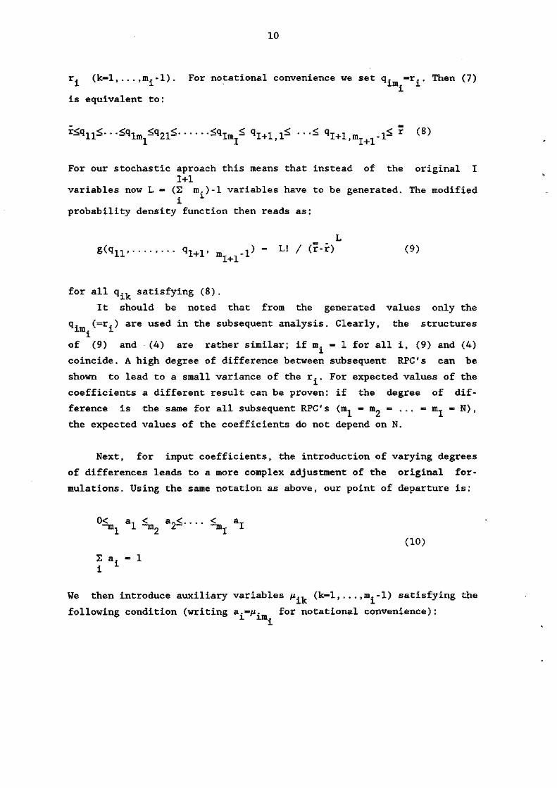
10
r. (k~l,...,m.-1). For notational convenience we set q. =r. . Then (7) i
is equivalent to:
r<qn<- . -<qlnii<q21< Ö l ^ qI+1>1< • • •< q ^ ^ . ^ r (8)
For our stochastic aproach this means that instead of the original I 1+1
variables now L = (2 m.)-l variables have to be generated. The modified i
probability density function then reads as:
L
«<*11 qI+l' mj+1-l> = L ! / <*"*> (9)
for all q., satisfying (8).
It should be noted that from the generated values only the
q. (=r.) are used in the subsequent analysis. Clearly, the structures i
of (9) and (4) are rather similar; if m. = 1 for all i, (9) and (4)
coincide. A high degree of difference between subsequent RPC's can be
shown to lead to a small variance of the r.. For expected values of the
coefficients a different result can be proven: if the degree of dif
ference is the same for all subsequent RPC's (nu — nu — ... - nu. — N),
the expected values of the coefficients do not depend on N.
Next, for input coefficients, the introduction of varying degrees
of differences leads to a more complex adjustment of the original for-
mulations. Using the same notation as above, our point of departure is:
0< a- < a„< < aT ~nu i ~nu /— ~mT
2 a. = 1 ï
1
(10)
We then introducé auxiliary variables /i-k (k-1 m.-l) satisfying the
following condition (writing a.=/i. for notational convenience):

11
0^11 < /i12. . . .<nlm^ < M 2 r • • - ^ m ^ - • • • ̂ Imj
(11)
2 fi. - 1 ï ï
It can be shovm that the modified probability density function f is
equal to:
I 1-1 m. f0*,, MT _ ,) - (( S m.)-l)! H (I+l-i) L (12)
' T" 1=1 ï=l
for all (*., satisfying (11). Note that when m. - 1 for all input coeffi-
cients, (12) coincides with (6). The approach described in Appendix I
can after some modifications be used again to generate random values
consistent with (12).
4.4 Ties and incomplete rankings
Ties deserve special attention in ordinal data; the probability
that ties occur is high in the case of a large number of ranked observa-
tions. Consider, for instance, the following ranking: a..< (a»,a„) < a, .
This may have different interpretations:
a„ and a- are exactly equal
a» and a_ are approximately equal
a„ and a_ are incomparable: a„ may be either larger or smaller than
a,, and the difference between the two is not necessarily small.
Each of these cases deserves its own treatment in the stochastic ap
proach outlined above.
When observations are exactly equal, one only needs to draw one
random value which is assigned to all observations concerned. An inspec-
tion of (9) and (12) reveals that this can be done in a consistent way
by interpreting an exact equality as <» (i.e., m. - 0 in such a case).
Thus, there is no need to design special procedures to deal with exact
equality: one can still use the formulas derived in Appendix I.
In the case of incomparable observations (an incomplete ranking)
one can still use the stochastic approach. Consider for example a
cluster of incomparable observations consisting of a„,a„ and a,. Then
random numbers x<y<z are generated which are assigned to a^.a- and a,

12
in a random way. Thus, in one case a„ may be assigned the largest value
(z), and in another case the smallest value.
In the case of approximately equal observations, one may proceed as
follows. In a first step, a value is generated for these observations as
if they were exactly equal (along the lines sketched above). In the
second step, the observations are assumed to be uniformly distributed in
an appropriately defined interval around this value. Consider for ex-
ample three clusters: {r, },{r-.r-} and {r,,r5} with the following
features: r,<r2=r-<r,«r,., where r2~r3 means that r„ and r, are ap
proximately equal. The Standard stochastic approach leads to values b1,
b„ and b- for the three clusters. Then in the last step, values for r0
I I and r, are drawn from a uniform distribution on the interval [•=• b- + •=
1 1 l i l b ? , -K b„ + ~2 t>33 • This approach can also be foliowed for input coeffi-
c i en t s , but in tha t case an addit ional condition (r„+r_ = 2b„) has to be
imposed to ensure that the add i t iv i ty const ra int on the coeff ic ients i s
s a t i s f i e d .
Thus in all cases the probability approach is in principle ap-
plicable and hence we may conclude that the stochastic approach outlined
above is quite flexible. It can deal with all kinds of ordinal data on
coefficients with and without additivity constraints:
Standard ordinal data
ordinal data with degrees of difference
ties of exactly equal observations
ties of approximately equal observations
incomparable observations.
Now the empirical question has to be answered whether the above men-
tioned approach leads to reliable results. This will be done in the next
section. 5. Empirical Results
The best way of testing empirically the reliability and ap-
propriateness of the ordinal input-output data method is to use an
existing quantitative input-output table, to transform it into ordinal
rankings of the coefficients and next to investigate whether our ordinal
data method is able to regenerate with a high degree of reliability the
information contained in the original table.
In our case the appropriateness of the method will be tested by
means of an existing regional input-output table. The table concerned is
that of the province of Groningen in the Northern part of the

13
Netherlands for the year 1980. The table is given in FNEI (1986) and
contains 9 sectors, one of which is the public sector. Household con-
sumption is also given which - in combination with the availability of
figures on wages and salaries as a fraction of value added - offers the
possibility of endogenizing the household sector.
Although this input-output table is published in quantitative
terms, a main part of it has a soft empirical basis. We have used types
of ordinal data as described in section 4 to represent the essential
characteristics of the underlying information. In the second step we
have used the stochastic approach of section 4 to generate random sets
of quantitative values consistent with these ordinal data. The different
verslons of the input-output tables are next compared by means of the
indirect income multipliers they generate. As we have seen in section
4 ordinalization can be carried out in various ways. Therefore two re-
lated questions may be asked: how well are multipliers estimated when
all ordinal information is incorporated in the procedure and how do the
various ways of formulating ordinal data affect the numerical results?
Both questions will be dealt with, but first we will discuss the or
dinalization phase itself.
The ordinalization we used is based on national input-output coef-
ficients together with regional purchase coefficients (RPC's). This
reflects the usual way regional tables are constructed. We assume here
that quantitative values of the value added coefficients are known for
each sector. Also some cells that by definition are zero in the original
table are set equal to zero in the estimated table at the outset. As
concerns the RPC's, we make a distinction between two vectors of RPC's,
one of which applies to the input coefficients and another one to
household consumption. We assume the availability of information on the
upper and lower bounds on both RPC vectors. RPC's that are known to be 1
are also assigned that value exogenously. Finally, wages and salaries as
a fraction of value added are also assumed to be known in a quantitative
way. Thus, the stochastic approach is applied to the input-output coef
ficients, including foreign imports, consumption coefficients and the
1 We have decided to evaluate the differences only by means of the indirect part of the multiplier, as the direct part is exogenously known. Comparing total multipliers underestimates the size of the differences at hand (cf. Oosterhaven et al, 1986)

14
RPC vectors. The results of our stochastic approach are sunmarized by
the mean values of the multipliers.
When we want to compare the indirect income multipliers based on
the ordinal data with the ones implied by the initial cardinal data, two
possibilities can be distinguished, depending on the way in which the
RPC's for the input coefficients are used. Starting with the national
input-output t'ble, the first possiMlity is multiplying each single
element with a separate RPC which leads to the given regional input-
output table. The second possibility is multiplying each element of a r r row with a common RPC. This means that in equation (2) r.. - r. for all ij i.
j. The first approach is obviously rather information demanding. The
second approach is more common practice but leads to less accurate mul
tipliers .
In our processing of the ordinal information we have only con-
sidered the case of one RPC per sector (row), as the treatment of RPC's
per cell is demanding too much information to be of any practical value
in the ordinal data approach. Of course, it is interesting to know what
the influence is of this simplification on our results, i.e., the sen-
sitivity of using sectoral RPC's per cell. Then it is also important to
know whether biases resulting from our ordinal data method show similar
patterns to the biases caused by the use of a sectoral RPC.
So we will first investigate the bias caused by the use of a sec
toral RPC by comparing multipliers based on the given input-output
table; see Table 1. This table shows multipliers from the original
regional input-output table, in which household consumption is treated
both exogenously and endogenously (columns 1 and 4, respectively).
Columns 2 and 5 show then the respective multipliers which result when
the national input coefficients are multiplied by sectoral RPC's. Next
columns 3 and 6 show the bias in columns 2 and 5 as a percentage of
column 1 and 4, respectively.

15
Table 1 Indirect income multipliers with RPC per sector and per cell
household consumption
exogenous
household consumption
endogenous
Sector (1) (2) (3) (4)
Cell Sectoral Relative Cell
RPC RPC diffe- RPC
rence
(5) (6)
Sectoral Relative
RPC difference
1. Agriculture .112 .092 -17.9 .452 .425 -6.0
2. Industry .468 .491 4.9 .917 .946 3.2
3. Utilities .651 .462 -29.0 1.157 .908 -21.5
4. Construction .377 .353 -6.4 .799 .766 -4.1
5. Trade .042 .045 7.1 .362 .363 0.3
6. Transport .077 .077 0.0 .407 .406 -0.2
7. Comm. services .153 .150 -2.0 .507 .501 -1.2
8. Other services .072 .066 -8.3 .401 .391 -2.5
9. Public sector .094 .094 0.0 .429 .427 -0.5
In general the bias resulting from the use of a sectoral RPC is
small, except for the sectors 1 and 3 (in case of exogenous household
consumption) and sector 3 (in case of endogenous household consumption).
More generally one observes a reduction in errors, when household con
sumption, being less sector-specific than intermediate demand, is
treated as an endogenous variable.
Table 2 shows the outcomes of the ordinal estimation procedure when
all types of ordinal information are used and when household consumption
is kept exogenous. The multipliers in the first column are those result
ing from the original cardinal input-output table (cf. Table 1). The
second column shows the mean value of the multipliers resulting from
using the ordinal data method 500 times, with their Standard deviation
in parentheses. Column 3 shorfs the bias of (2) as a percentage of (1).

16
Table 2. Indirect income multipliers with exogenous household con-
sumption.
Initial Ordinal data method
(n = 500)
Sector (1) (2) (3) (4)
Relative
mean stand difference
dev. between (1)
and (2) (in %)
1. Agriculture .112 .099 (.025) -11.6
2. Industry .468 .499 (.142) 6.6
3. Utilities .651 .672 (.159) 3.2
4. Construction .377 .415 (.055) 10.0
5. Trade .042 .057 (.048) 35.7
6. Transport .077 .083 (.026) 7.8
7. Comm. services .153 .155 (.013) 1.3
8. Other services .072 .068 (.009) -5.6
9. Public sector .094 .090 (.011) -4.3
Table 2 shows that the Standard deviations as generated by the ordinal
approach are rather large, in most cases (far) over 10% of the respec-
tive means. All initial multipliers are within the interval of mean + or
Standard deviation. More interesting is the fact that the ranking of
the multipliers with respect to their magnitude is the same in both
cases. This means, for instance, that the sector with the largest multi
plier effect is correctly identified. The biases do not follow a clear
pattern, although we note that really large biases (over 20%, for
instance) are rare. When we compare column (4) of Table 2 with column
(3) of Table 1, there is no indication that the biases in our qualita-
tive data method are a consequence of the use of sectoral RPC.
Table 3 shows multipliers when household consumption is made endogenous.
Again all types of ordinal information are used.

17
Table 3. Indirect income multipliers with endogenous household
consumption.
Initial Ordinal data method (n = 500)
Sector (1) (2) (3) (4)
mean stand dev.
Relative difference between (1) and (2) in %
1. Agriculture .452 .456 (.054) 0.9
2. Industry .917 1.003 (.181) 9.4
3. Utilities 1.157 1.229 (.198) 6.2
4. Construction .799 .864 (.091) 8.1
5. Trade .362 .399 (.050) 10.2
6. Transport .407 .438 (.054) 7.6
7. Comm. services .507 .529 (.051) 4.3
8. Other services .401 .415 (.046) 3.5
9. Public sector .429 .445 (.047) 3.7
The results of Table 3 are quite similar to those of Table 2. Again
almost all Standard deviations appear to be over 10% of the means and
again all initial multipliers are within a range of mean + or - Standard
deviation. Column (4) of Table 3 and column 6 of Table 1 do not display
a similar pattern. The only remarkable result of Table 3 is that all
initial multipliers are (slightly) overestimated by the ones of the
ordinal data method. There is no intrinsic reason why this should be the
case. It is an accidental result of the way the initial coefficients
have been reformulated in ordinal terms. Finally, we note that - even
though there is a cluster of initial multipliers which have a similar
order of magnitude - the ranking of the multipliers is again correctly
'predicted' by the ordinal data method.
Next we discuss the various stages of adding new information on our
data. In Table 4 the following cases are distinguished. In the base case
the ordinalization is carried out without allowing ties or degrees of
differences. In the "•»" case the base case is extended with the al-
lowance of ties which are all interpreted as 'equal to'. The "»" case is
similar to the "«" case, but now with ties interpreted as 'approximately

18
equal to'. In the 'both' case both interpretations of ties are allowed
for. In the case labelled 'DOD' again no ties are allowed, but in that
case we make use of the concept of degree of difference. Finally, in the
case of label 'ALL', all types of ordinal information are used simul-
taneously.
In the present context where quantitative guesses of coefficients
are already available, the interpretation of ties as being imcomparable
is not relevant, and hence we decided to drop this interpretation in the
experiments reported here.
Table 4. Effect of extra information on mean values of multipliers
(initial multiplier — 100); household consumption en-
dogenous; (n*=500) .
Sector Base = ~ Both DOD ALL
1. Agriculture 108 105 104 104 105 101
2. Industry 136 127 127 128 119 109
3. Utilities 140 135 134 136 109 106
4. Construction 112 111 110 110 110 108
5. Trade 122 117 117 117 118 110
6. Transport 108 104 104 103 112 108
7. Comm. services 100 97 97 96 107 104
8. Other services 98 96 96 96 106 103
9. Public sector 100 97 97 97 107 104
mean absolute 14 12 12 12 10 6
percentage error
Table 4 shows some interesting results. First, the way in which
ties are interpreted does not make any significant difference for the
results. Second, there is a significant difference in the dispersion in
index values of the DOD and ALL cases compared to the other cases.
Third, the ALL case appears to give the best estimates, although only
with respect to the average of the index numbers and not for the last
three sectors. We will discuss these results in more detail below.
From the discussion in section 4 it can be derived that the way in
which a tie is interpreted does not make any difference for the mean
value of a single element which is drawn. At the same time it appears to
be impossible to derive analytically the distribution function of the

19
multipliers involved because of the stochastically complex operations of
multiplication and inversion that have to be carried out in order to
arrive at the multipliers. Table 4 now shows that the mean values may be
considered identical (the small differences can be attributed to sam
pling effects), while Table 5 shows that also the Standard deviations
are very much similar (for the sake of completeness the Standard devia
tions of the other cases are also given).
Table 5. Effect of extra information on Standard deviations of
multipliers; bousehold consumption endogenous; (n=500).
Sector base = ~ both DOD ALL
1. Agriculture .065 .070 .066 .068 .056 .054
2. Industry .183 .227 .224 .212 .170 .181
3. Utilities .287 .311 .308 .296 .196 .198
4. Construction .114 .114 .119 .117 .091 .091
5. Trade .061 .067 .064 .067 .051 .050
6. Transport .065 .065 .063 .066 .054 .054
7. Comm. services .062 .064 .063 .064 .052 .051
8. Other services .057 .058 .056 .058 .048 .046
9. Public sector .058 .060 .058 .060 .048 .047
Thus in an empirical sense the distinction between the various ways
of dealing with ties is apparently not necessary. This means that all
ties may be considered as 'equal to' ties which are computationally
easier to handle.
We checked the above statement by generating multipliers allowing
for degrees of differences, by combining them with various interpreta-
tions of ties. The hypothesis that the various ways of dealing with ties
are redundant leads to the expectation that the cases of DOD plus "-"
and DOD plus "«" both give multipliers more or less identical to the
'ALL' case. It turned out that indeed the mean values of the multipliers
were in all three cases almost identical (the difference in index num
bers was 1 point at most), while also the Standard deviations were very
much alike.
Returning to the results of Table 4, we already noted the dif-
ference in dispersion in the index numbers of the 'ALL' case compared
to the other cases. Of course a situation where all multipliers are

20
estimated with the same error is preferable to a case where some multi
pliers are estimated without any error and some others with rather large
errors, especially when it is not known which multipliers are wrongly
estimated. This observation makes clear that all available information
should be incorporated when using the ordinal data method. But examining
the underlying multipliers reveals an even more important result, viz.
that the ranking of the multipliers is only correctly generated by the
'ALL' case (cf. Table 3). This statement was checked by also examining
in an analogous way the multipliers resulting from the various cases of
the information used, when household consumption was kept exogenously.
Also these results appear to confirm the above conclusion. Only in the
case when all information is used, the ranking of the multipliers gener
ated is the same as in the initial case. Thus we may conclude that the
ALL case is the only one giving a correct picture of the quantitative
structure of the economy.
6. Conclusion
Quantitative economie analysis aims at deriving conclusions with a
maximum degree of reliability. If in a given case no cardinal data are
available nor can be obtained in the framework of a certain research
project and if instead ordinal data are available, then good practice
means to derive as much information as possible from the existing data
set. The ordinal data method described in this paper and applied in the
framework of input-output analysis has clearly shown that this is a
meaningful endeavour which - by generating cardinal figures out of or
dinal data - generates numerically plausible results. In the test case,
where original and re-generated cardinal data are compared, it appears
that the point estimates are satisfactory when all available information
is used. The errors of an ordinal input-output analysis appear to be
relatively small, for instance, in comparison to errors when alternative
updating procedures are used (see Oosterhaven 1986).
In input-output analysis one of the ways often used to overcome the
problem of missing quantitative data is to use expert judgements to
arrive at cardinal values of the coefficients concemed. The reliability
of the ensueing multipliers is questionable however. The ordinal ap-
proach presented here is an attractive alternative since the Standard
deviations it generates are a useful means to judge the range of uncer-
tainty on the multipliers because of data weaknesses. The ordinally
estimated multipliers however, should not (or not necessarily) replace

21
the cardinal ones. Also, it is preferable to use hard (cardinal) infor-
mation whenever possible, very much in the same way as we used the value
added coefficients. Our method is able to cope with this kind of mixed
data.
Concerning the technical part of the method , the interesting
result emerges that in this case study the interpretation of ties
('equal to' versus 'approximately equal to') is not important. On the
other hand, the concept of degree of differences appears to be essential
for the use of our method.
The main advantage of ordinal input-output analysis is the integra-
tion of input-output table construction and the determination of
Standard errors into one framework. Our analysis has demonstrated -
based on an empirical test case - that ordinal input-output analysis may
offer an extremely valuable alternative in case of missing or imprecise
information on technical coefficients in an input-output model.

22
Appendix I Generating Random Values for Regional Purchase
Coefficients and Input Coefficients
1. Generating regional purchase coefficients
As indicated by Mood and Graybill (1963), it is not difficult to
generate random values for r,,...,r_. They show by means of order
statistics that one can start with drawing I numbers from the uniform
distribution on [0,1], after which r.. is assigned the smallest number,
r„ the one but the smallest number, etc.
An alternative approach would be the following one. Taking (4) as a
starting point, it can be shown that the marginal distribution of the
smallest RPC reads as follows:
1-1 _ I g(rx) - I (r-r^ /( r - r ) r < *1 < r
— 0 elsewhere
Further, the conditional density functions can be shown to read as fol
lows for i - 2,...,I:
I-i _ I-i+1 g(ri|r1, . . . ,ri;L) - (I-i+1) (r-r^ /(r-r^)
where r. n < r. < r i-I - ï _
Thus, a random vector with RPC's can be generated by drawing a value for
r. on the basis of g(r-), foliowed by drawing a value for r„ on the
basis of g(r«|r1), etc. However, these conditional distributions are not
included in Standard statistical packages. Therefore, random values
cannot be directly created by means of random generators. A solution for
this problem is given by the theorem which says that if G(x) is the
distribution of x, then u = G(x) is uniformly distributed on the inter
val 0 < u < 1 (Hogg and Craig, 1970, p. 349). For the latter uniform
distribution, Standard random generators are available. Then if u, is
uniformly distributed on the interval [0,1], r.. — G (u^) can be shown
to be distributed according to the density function g(r1). Thus, random
values for r, can be found by using the following transformation:

23
rx - r- ( r - r ) (1-u)1/1
For i- 2....I, the following transformation has to be used:
r r r - (r-ri;L) (l-u) 1 / I _ i + 1
2. Generating input coefficients
The starting point is the joint density function of input coeffi-
cients:
f (a1,...,aI_1) - c 0< a± < 1/1
ax< a2 < (l-ai)/(I-l)
a2< a3 < (l-ai-a2)/(I-2)
aI-2 ~ aI-l ~ (1_ai>"-•-"ai.2^/2
— 0 elsewhere
where c - (I-1)!I!
Then the marginal density function of a- can be derived as:
f(a1)-(I-l)I(l-Ia1)1"2 for 0< a1 < (1/1)
- 0 elsewhere
Furthermore, the conditional density functions can be shown to read as
follows for i - 2,...,I-1
[1-a -,-...-a -(I-i+Da.]1"1"1
- (I.1)(.I-I+1) — =-f-[1-a^...- (I-i+2)ai_1]
i":L
where a. , < a. < (1-a., -...- a. , )/(I-i+l)
Then a random vector with input coefficients can be generated by drawing
a value for a» on the basis of f(a,), foliowed by drawing a value for a„

24
on the basis of f(a„|a,), etc. Finally, a_ can be computed as 1-a- ...-
aI-l'
Let again u. be a number drawn from the uniform distribution on the
interval [0,1]. Then it can be shown that the following transformation
has to be used to generate random values of a.. :
For a„,...,aT 1 the following transformation has to be used:
at - [(l-a1-...-ai_1)-(l-a1-...-ai_2-(I-i+2)ail)(l-ui)1/(I"i)]/(I-i+l)
Finally, ay can be computed as l-a..-...-aT - .

25
References
Bon, R., 1989. Qualitative Input-Output Analysis. In Frontiers of Input-Output Analvsis. eds. R.E. Miller, K.R. Polenske and A.Z. Rosé, Oxford University Press, New York, pp. 221-231.
Brouwer, F., J. Maybee, P. Nijkamp and H. Voogd, 1989. Sign-Solvability in Economie Models through Plausible Restrictions, Atlantic Economie Journal. vol. 17, no. 2, pp. 21-27.
FNEI, 1984a. De Interregionale Input-Output Tabel voor Drenthe- Overig Nederland 1975, Federatie voor Noordelijke Economische Instituten, Assen.
FNEI, 1984b. De Interregionale Input-Output Tabel voor Groningen- Overig Nederland 1975, Federatie voor Noordelijke Economische Instituten, Groningen.
FNEI, 1985. De Interregionale Input-Output Tabel voor Friesland- Overig Nederland 1975, Federatie voor Noordelijke Economische Instituten, Leeuwarden.
FNEI, 1986. Input-Output Tabellen voor Groningen, Friesland, en Drenthe; Actualisatiemethoden en Analyse, Federatie voor Noordelijke Economische Instituten, Assen.
Hewings, G.J.D., 1977. Evaluating the Possibilities of Exchanging Regional Input-Output Coefficients, Environment and Planning A 9, pp. 927-944.
Hogg, R.V., and A.T. Craig, 1970, Introduction to Mathematical Statistics. MacMillan, London.
Isard, W., 1960. Methods of Regional Analvsis : An Introduction to Regional Science. The Technology Press of MIT and John Wiley Sons, Inc., New York.
Jackson, R.W. en G.R. West, 1989. Perspectives on Probabilistic Input-Output Analysis. In Frontiers in Input-Output Analvsis. eds. R.E. Miller, K.R. Polenske and A.Z. Rosé, Oxford University Press, New York, pp. 209-221.
Jensen, R.C. and S. MacDonald, 1982. Technique and Technology in Regional Input-Output, The Annals of Regional Science 15, 2, pp. 27-45.
Katz, J.L. and R.L. Burford, 1981. A Method of Estimating of Input-Output Multipliers when no I-O Model Exists. Journal of Regional Science 21, pp. 151-161.
Lahiri, S. and S. Satchell, 1986. Properties of the Expected Value of the Leontief-Index: Some Further Results, Mathematics for Social Science 11, pp. 69-82.
Lancaster, K., 1981. Maybee's 'Sign Solvability', Computer-Assisted Analysis and Model Simplification (H.J. Greenberg and J.S. Maybee, eds.), Academie Press, New York, pp. 259-270.

26
Lazarsfeld, P.F., and A. Burton, 1971. Qualitative Measurement in the Social Sciences, Research Methods: Issues and Insights (B.J. Franklin and H.W. Osborne, eds.), Wadsworth Publ. Co., Belmont, Cal., pp. 140-160.
Lecomber, J.R.C., 1975. A Critique of Methods of Adjusting, Updating and Projecting Matrices. In Estimating and Proiecting Input-Output Coefficients. eds. R.I.G. Allen and W.F. Gossling, Input-Output Publishing Company, London, pp. 1-25.
Leontief, W.W. and A. Strout, 1963. Multiregional Input-Output Analysis. In Structural Interdependence and Economie Development. ed. T. Barna, MacMillan, London, pp. 119-149.
Manski, C.F. and D. McFadden (eds.), 1981. Structural Analvsis of Discrete Data with Econometrie Applications. MIT Press, Cambridge, Mass.
Miller, R.E. and P.D. Blair, 1985. Input-Output Analvsis: Foundations and Extensions. Prentice Hall, Englewood Cliffs, NJ.
Mood, A.M., and F.A. Graybill, 1963. Introduction to the Theorv of Statistics. McGraw-Hill, New York.
Nijkamp, P., H. Leitner and N. Wrigley (eds.), 1985. Measuring the Unmeasurable. Kluwer Nijhoff, Dordrecht.
Oosterhaven, J., 1979. Construction of an Interregional Input-Output Table for the North, the Rijnmond Area and the Rest of the Netherlands for 1970. Memorandum nr. 54. Institute for Economie Research, University of Groningen, Groningen.
Oosterhaven, J., G. Piek and D. Stelder, 1986. Theory and Practice of Updating Regional versus Interregional Interindustry Tables. Papers of the Regional Science Association 59, pp. 57-72.
Richardson, H.W., 1972. Input-Output and Regional Economics. Weidenfeld and Nicolson, London.
Richardson, H.W., 1985. Input-Output and Economie Base Multipliers: Looking Backward and Forward. Journal of Regional Science 25, 4, pp. 607-661.
Rietveld, P., 1984. The Use of Qualitative Information in Macro-Economie Policy Analysis, in: Macro Economie Planning Conflicting Goals. M. Despontin et al. (eds.), Springer, Berlin, pp. 263-280.
Rietveld, P., 1989. Using Ordinal Information in Decision Making under Uncertainty, Systems Analvsis. Modeling Simulation. vol. 6, pp. 659-672.
Roberts, F.S., 1979. Measurement Theorv. Addison-Wesley, Reading, Ma.
Round, J. I., 1978. On Estimating Trade Flows in Interregional Input-Output Models. Regional Science and Urban Economics 8, 3, pp. 289-302.

27
Saaty, T.L., 1977. A Scaling Method for Priorities in Hierarchical Structures, Journal of Mathematical Psvchologv. vol. 15, pp. 234-281.
Samuelson, P.A., 1947. Foundations of Economie Analvsis. Harvard University Press, Harvard.
Sonis, M. and G.J.D. Hewings, 1989. Error and Sensitivity Input-Output Analysis: New Approach. In Frontiers of Input-Output Analvsis. eds. R.E. Miller, K.R. Polenske and A.Z. Rosé, Oxford University Press, New York, pp. 232-244.
Stevens, B.H., 1987. Comments on 'Ready Made' Regional Input-Output Model Systems: Model Accuracy and the Value of Limited Surveys. Review of Regional Studies 17, 1, pp. 17-20.
Stevens, B.H., G.I. Treyz and M.L. Lahr, 1989. On the Comparative Accuracy of RPC Estimating Techniques. In Frontiers of Input-Output Analvsis, eds. R.E. Miller, K.R. Polenske and A.Z. Rosé, Oxford University Press, New York, pp. 245-257.
Taha, H.A., 1976. Operations Research. MacMillan, New York.
Uno, K., 1989. Measurement of Services in an Input-Output Framework. North-Holland, Amsterdam.
West, G.R., 1986, A Stochastic Analysis of an Input-Output Model, Econometrica 54: pp. 363-374.

1989-1 O.J.C. Cornlelje
1989-2 J.C. van Ours
00 CM
1989-3 H. Visser
1989-4 G.van dar Laan A.J.J. Talnan
1989-5
1989-6
H.M. van Dijk
N.M. van Dijk
1989-7 P.Spreij
1989-8 H.Visser
1989-9 J.C. van Ours
1989-10 H. Tieleraan A. Leliveld
1989-11 H.M. van Dijk
1989-12 F.A.G. den Butter
1989-13 H.M. van Dijk
1989-14 H. Clemena J.P. de Groot
1989-15 I.J.Steyn
1989-16 I.J.Steyn
1989-17 B.Vogelvang
1989-18 J.C. van Ours
A time-series of Total Accounts for the He-therlands 1978-1984
Self-Service Actlvities and Lega.1 or Illegal Market Services
The Monetary Order
Price Rigidities and Ratloning
A Simple Throughput Bound For Large Cloaed Queueing Networks Wlth Finlte Capacities
Analytic Error Bounds For Approximationa of Queueing Networks with an Application to Alternate Routing
Selfexciting Counting Process Systems with Finlte State Space
Rational Expectatlons and New Classlcal Macroeconomics
De Nederlandse Boekenmarkt tussen Stabiliteit en Verandering
Traditional "Social Security Systems" and Socio-economic Processes of Change: The Chase of Swaziland; opportunities for research
"Stop - Recirculate" for Exponential Product Form Queueing Networks with Departure Bloc-king
Modelbouw en matigingsbeleid in Nederland
Simple performance estimates and error bounds for slotted ALOHA loss systems
Sugar Crisis, a Comparison of two Small Pe-ripheral Economles
Consistent Diffuse Initial Conditions in the Kalman Filter
Als Estimatlon of Parameters in a State Space Model
Dynamic Interrelatlonships between Spot Pri-ces of some Agrlcultural Commodities on Rela-ted Markets
Zoeken naar nieuwe medewerkers
1989-19 H. Kox Integration of Envlronmental Externalltles in International Commodity Agreements
1989-20 P.B.F.M. van Casteren A.H.Q.M. Herkies
1989-21 J.C. van Ours
1989-22 R.J.Boucherle H.M. van Dijk
1989-23 N.M. van Dijk
1989-24 A.F.de Voa J.A. Bikker
1989-25 A.F. de Vos
1989-26 N.H. van Dijk
1989-27 H.Clemena
1989-28 N.M. van Dijk F.J.J. Trapman
1989-29 N.M. van Dijk
1989-30 A. Perrels
1989-31 J.C. van Ours 0.Ridder
1989-32 N.M. van Dijk
1989-33 A. v.d. Elzen G. v.d. Laan
1989-34 N.M. van Dijk
1989-35 H.Visser
1989-36 N.M. van Dijk
1989-37 A.F. de Vos
1989-38 R.J. Hulskamp
1989-39 Dr. Raul Ruben