Improving the prediction of soccer match results

by means of Machine Learning

Joost Hessels

Master Thesis Data Science ‘Business & Governance’

Supervisor: prof. dr. E.O. Postma

Second reader: dr. W. Huijbers

Tilburg University

School of Humanities

Department of Communication and Information Sciences

Tilburg, The Netherlands

August 2018

2

Preface

This thesis is the final product of my master Data Science ‘Business & Governance’ at Tilburg University.

The completion of this thesis would not have been possible without the following people. First of all, I wish

to thank my supervisor prof. dr. Eric Postma for his guidance, pragmatic advice, and insightful feedback.

Furthermore, I would like to thank my fellow master students and friends Janno, Tom, Mariette, Coen, and

Amber for the coffee and lunch breaks, keeping me motivated, and for all the great moments we have

experienced together during our master period. Last but not least, I would like to express my love and

appreciation for all the support and encouragement from my parents, my sister, my friends, and in particular

by Maudy.

I hope you enjoy your reading.

Joost Hessels

Tilburg, August 2018

3

Abstract

In this study, we predict the full-time results (FTR) of soccer matches in the English Premier League,

Championship, League One, and League Two using data science and machine learning. The main goal of

this study is to improve upon the prediction results of Ulmer et al. (2013) by using a bigger dataset. An

additional goal is to engineer and evaluate novel features to enhance the prediction accuracy. Our target

feature FTR consists of three possible classes: Home win (H), Draw (D), and Away win (A). The classifiers

Random Forest and Support Vector Machine (SVM) are used for this classification problem. Match statistics

datasets of the 2002/03 season until the 2017/18 season are retrieved from Football-Data.co.uk. We

determined that the match statistics regarding shots on target are most informative for predicting soccer

match results. By applying feature extraction to the datasets, we engineered new features: team strength,

team ranking, cumulative sum, goal difference, form, weighted form, and differential. The feature set which

contained only differential features yielded best prediction results. Both Random Forest (0.57) and SVM

(0.59) outperformed the accuracy scores of Ulmer et al. (2013), who obtained 0.50 and 0.51. Furthermore,

we extended our dataset season-based, which resulted in our best prediction result using SVM: accuracy of

0.60. In contrast, division-based extending of the dataset resulted in a decrease in the predictive ability of

the classification models.

[Keywords] Soccer Match Results Prediction • Football-Data • English Professional Soccer • Premier

League • Championship • League One • League Two • Data Science • Data Mining • Machine Learning •

Classification • Random Forest • SVM • R

4

Contents

Preface ........................................................................................................................................................... 2

Abstract ......................................................................................................................................................... 3

Contents ......................................................................................................................................................... 4

Introduction ................................................................................................................................................... 6

Research Questions ................................................................................................................................... 8

Structure .................................................................................................................................................... 9

Related work ............................................................................................................................................... 11

The Ulmer et al. (2013) study.................................................................................................................. 11

Other studies ............................................................................................................................................ 11

Our Prediction Method ............................................................................................................................ 16

Original Features ................................................................................................................................. 16

Engineered Features ............................................................................................................................ 16

Classifiers ............................................................................................................................................ 18

Method ........................................................................................................................................................ 19

Dataset ..................................................................................................................................................... 19

Software .................................................................................................................................................. 19

Pre-Processing ......................................................................................................................................... 19

Data Cleaning ...................................................................................................................................... 19

Target Feature...................................................................................................................................... 20

Feature Selection ................................................................................................................................. 22

Feature Extraction ............................................................................................................................... 22

Experimental Setup ................................................................................................................................. 25

Experiment 1 ....................................................................................................................................... 25

Experiment 2 ....................................................................................................................................... 26

Experiment 3 ....................................................................................................................................... 26

5

Experiment 4 ....................................................................................................................................... 27

Evaluation ................................................................................................................................................ 29

Results ......................................................................................................................................................... 30

Experiment 1 ........................................................................................................................................... 30

Experiment 2 ........................................................................................................................................... 31

Experiment 3 ........................................................................................................................................... 32

Experiment 4 ........................................................................................................................................... 34

Discussion, Conclusion & Future Work ...................................................................................................... 38

Discussion ............................................................................................................................................... 38

Conclusion ............................................................................................................................................... 39

Future Work ............................................................................................................................................ 42

References ................................................................................................................................................... 44

Appendix A ................................................................................................................................................. 47

6

Introduction

Several times in the history of soccer, the world was shocked by results that were considered previously as

impossible. The most remarkable recent example is about Leicester City’s fairytale story in the 2015/16

season of the Premier League, which is England’s highest soccer division. Leicester City succeeded in

winning the Premier League, while before the season started the odds for Leicester City to win the league

were one against 5000. Until then, Leicester City had never won a top-flight title in its 132-year existence.

The most unimaginable about this fairytale is that Leicester City was at the bottom of the Premier League

in April 2015, nevertheless managed to avoid relegation to the second division in their last matches, to

subsequently become champions of England around a year later. Incidentally, all this did not happen as a

result of large financial investments by a wealthy club owner, but through smart transfer policy and by

putting team interest in the first place. Moreover, the manager of Leicester City in the 2015/16 season was

the Italian Claudio Ranieri, who was sacked as manager of the Greece national team half a year earlier after

losing against the Faroe Islands. Speaking of the Greece national team, they also managed to realize

something which was held as very unlikely to happen. They won the European Championship in 2004 as

outsiders after beating Portugal, which hosted the tournament, in the final in Lisbon. Even though no other

soccer story in terms of impact is comparable to the Leicester City fairytale, a European Championship

winner whose odds in advance were estimated at one against 150, can rightly be seen as an unbelievable

performance.

Soccer is completely unpredictable, more so than any other sport. It is so unpredictable that Bradford

can go to Chelsea and win. – Arsène Wenger (Manager Arsenal FC)

These fascinating stories show that soccer is a very unpredictable sport. In contrast to a single match that

went differently than predicted in advance, the unique achievements of Leicester City and the Greece

national team were examples of a series of matches that, against all the odds, turned out to be a success for

the underdog. Even though predicting soccer match results is not an easy task, the words of Arsène Wenger,

cited above, provide ample motivation. Contradictory to Arsène Wenger’s judgment, the goal of this study

is to be able to predict the results of soccer matches correctly by means of data science.

The application of data science is becoming more and more popular in soccer. Many soccer clubs realize

that when data is used properly, this could bring them steps ahead of their competitors. Data analytics and

the application of machine learning techniques is interesting for different tasks in soccer, such as monitoring

the physical health of players (Rossi et al., 2017), scouting players based on their predicted potential

7

(Vroonen, Decroos, van Haaren, & Davis, 2017), discovering playing styles of opponents (Wang, Zhu, Hu,

Shen, & Yao, 2015), and betting on match events and match results (Snyder, 2013). The latter task, betting

on match results, is part of the financial aspect of soccer matches considering that the soccer betting industry

is worth almost two billion dollars each year1. This is due to the fact that soccer is by far the world’s leading

sport with over four billion followers2. In addition, an average Premier League match has a global audience

of more than twelve million people3. Moreover, the Championship, England’s second division, is the third

most-watched league in European soccer, which is more than the viewing density of the Spanish La Liga,

Italian Serie A, and French Ligue 14. In short, the societal relevance of our research problem is evident and

motivated us to predict match results in English professional soccer. More specifically, we focus on the four

highest soccer divisions in England, namely the Premier League, Championship, League One, and League

Two.

From a scientific perspective, multiple studies showed that it is not a straightforward task to predict soccer

match results because of a large number of factors that can influence a match result. For instance, the relative

roles of skill and luck in soccer has been investigated by Aoki, Assuncao, and Vaz de Melo (2017). They

demonstrated that only a carefully selected 25% of the teams of the Premier League need to be removed in

each season to create a completely random competition. In other words, 15 teams of the Premier League are

competitively equivalent to each other, which makes it challenging to predict match results correctly.

Nevertheless, many studies met the challenge by creating prediction models that were trained and tested on

data from the Premier League (Baboota & Kaur, 2018; Constantinou, Fenton, & Neil, 2012; Gomes, Portela,

& Santos, 2015; Razali, Mustapha, Yatim, & Ab Aziz, 2017; Ulmer, Fernandez, & Peterson, 2013). One of

the best prediction results obtained were reported by Ulmer et al. (2013): 51% correctly predicted match

results. Notice that each soccer match has three possible Full-Time Results, which we call FTR: Home win

(H), Draw (D), and Away win (A). Given that this result is better than chance, it indicates that there is

something to gain from data science. There is no need to explain that the use of statistical models is common

regarding soccer match result predicting. Despite, this study focusses on predicting match results by means

of machine learning. This is decided based on the fact that the study of Ulmer et al. (2013), which we want

to improve upon, relies on machine learning techniques as well as based on our own interests within the

data science domain.

Regarding the study of Ulmer et al. (2013), one of the main limitations was the relatively small amount of

available data from earlier seasons. Therefore, as future work for their study, they recommended using more

1 Source: https://www.mirror.co.uk/sport/football/news/football-betting-worth-14billion-gambling-10498762 2 Source: https://www.totalsportek.com/most-popular-sports/ 3 Source: https://contexts.org/articles/english-soccers-mysterious-worldwide-popularity/ 4 Source: https://www.bbc.com/sport/football/42704713

8

data for training prediction models. Specifically, Ulmer et al. (2013) stated that using more data from that

time period, such as statistics from previous matches and the quality of attack and defense, would lead to an

improvement of the predictive ability of their model. This is interesting since accurate soccer match datasets

are available for the last fifteen seasons of the four highest divisions in England. Because of this, we decided

to predict the FTR of matches in English professional soccer using more data. The main goal of this study

is to improve the results of Ulmer et al. (2013) by using a bigger dataset. An additional goal is to develop

and evaluate novel features to enhance the prediction accuracy.

In our study, we have access to soccer match data from the 2002/03 season until the 2017/18 season of the

four highest divisions in English professional soccer, whereas the dataset of Ulmer et al. (2013) contained

only data from the 2002/03 season until the 2013/14 season of the Premier League. This allows us to

replicate and extend their study using a bigger dataset encompassing more soccer matches. Furthermore, the

dataset of Ulmer et al. (2013) consisted of only the FTR and the number of goals scored by each team per

match, whereas our dataset also contained match statistics for each team, such as the number of shots on

target, the number of corners, and the number of cards. Hence, we are able to replicate their study using new

features, which are engineered on the basis of match statistics.

In order to improve upon the study of Ulmer et al. (2013), we decided to keep our investigation similar and

focus on the two best-performing algorithms in their study: Random Forest and Support Vector Machine

(SVM). Therefore, this study does not incorporate with other classifiers, for instance, Bayesian Networks,

which are commonly applied with regard to match result prediction (Razali, Mustapha, Utama, & Din,

2018). As each soccer match has three possible match results, our prediction task with FTR as target feature

is a multi-class classification problem where chance level normally would be 33%. However, the percentage

of the majority class, which is a win for the home team (H) relative to all possible classes (H | D | A), is

approximately 44%. Since predicting all match results as class H would generate an accuracy score of 0.44,

this is our baseline for prediction. Although our study focusses on English professional soccer, our

developed prediction model is easily applicable to other soccer competitions provided that the same type of

data about match statistics is available.

Research Questions

In this study, we addressed the following problem statement:

To what extent can we improve upon the prediction results of Ulmer et al. (2013)?

In order to formulate an answer to this problem statement, we formulated four research questions, which

will be discussed in the next paragraphs.

9

To start with, being able to validate our prediction results relative to the study of Ulmer et al. (2013), we

first had to replicate their prediction models. Hence, the first research question reads as follows:

RQ 1: To what extent can we replicate the study of Ulmer et al. (2013)?

For this investigation, a dataset containing soccer match statistics is used to predict the FTR of soccer

matches. This dataset, which we call the original dataset, consisted of the number of shots, shots on target,

fouls, corners, yellow cards, and red cards that occurred in a match for both the home and away team. The

second challenge of this study was to determine which of these match statistics of the original dataset, which

we call original features, are most informative regarding match result prediction. In order to identify which

original features are most predictive regarding match results, the second research question reads as follows:

RQ 2: Which original features are most informative for predicting match results?

Based on the results of the experiment to answer the second research question, feature selection is applied.

Subsequently, the selected original features are used to create new features through feature extraction, which

we call engineered features. These engineered features, which are gathered into our engineered dataset, are

constructed by relying on ideas from related studies (Baboota & Kaur, 2018; Ulmer et al., 2013) and based

on our understanding of the problem domain. We attempted to improve upon the study of Ulmer et al. (2013)

by means of the newly created engineered features which are expected to be more informative than the

features they used. Therefore, the third research question reads as follows:

RQ 3: To what extent does the addition of engineered features contribute to the prediction of

match results?

Apart from the fact that the dataset that is used in this study contained a larger variety of original features

than the dataset of Ulmer et al. (2013), we also had access to data of more soccer matches. The use of more

soccer matches could lead to an increase in the predictive ability of the model. Therefore, the effect of

extending the size of the dataset is investigated. Hence, the last research question reads as follows:

RQ 4: To what extent does the extension of the dataset contribute to the prediction of match

results?

Structure

The remainder of this thesis is organized as follows. The first chapter provides an overview of related work

which already has been performed. After the Related Work chapter, the Method chapter follows, which

describes the dataset and experimental setup of this study. The performance of the model is presented in the

Results chapter. The last chapter of this thesis consists of the Discussion section, the Conclusion section,

10

and the Future Work section. In the Discussion, our findings are used to refer back to the goal of the study

and used to put this study in perspective regarding other literature. In the Conclusion section, the research

questions will be answered. Finally, we suggest future work based on the implications of this study.

11

Related work

This chapter briefly specifies the study which we attempt to improve, describes related work that is

conducted, including an overview of these studies, and defines our prediction method.

The Ulmer et al. (2013) study

Ulmer et al. (2013) used soccer match data from the 2002/03 season until the 2011/12 season to train their

model in order to predict match results of the 2012/13 and 2013/14 season of the Premier League. They

used home advantage, team ranking, form and weighted form over match results, and goal difference as

features. The form over match results represents the performances of each team over the previous matches.

The weighted form is calculated by adding separate weights to the form. Ulmer et al. (2013) found that the

optimal number of matches to aggregate the form over was 7 when Random Forest was applied, whereas 4

led to better results using SVM. The hyperparameters of the prediction model were tuned using a grid search

with 5-fold Cross-Validation. The optimal values for the hyperparameters of Random Forest were 110 as

the number of estimators and 2 as the minimum number of examples required to split an internal node. In

regard to SVM, the optimal value for C was 0.24, and for gamma 0.15. As stated, Ulmer et al. (2013)

achieved an accuracy score of 0.50 using Random Forest, and 0.51 using SVM, that we attempted to improve

upon. In order to avoid overfitting, they maintained experimenting until the error on the training data and

the test data were close to each other. Ulmer et al. (2013) encountered that reducing the complexity of their

prediction models resulted in the prevention of overfitting.

Other studies

This section reviews related work on match result prediction. We confine our review to studies that rely on

data from the Premier League, or that applied Random Forest or SVM. In what follows, we review five

studies.

First, Razali et al. (2017) predicted the FTR of soccer matches using Bayesian Networks, as well as

Constantinou et al. (2012). Data from the 2010/11 season until the 2012/13 season of the Premier League

was selected. As features for the prediction model, Razali et al. (2017) used the match statistics which we

call original features. As a matter of fact, their model is not applicable to predict the FTR of future soccer

matches. Given our second research question, it would have been interesting if Razali et al. (2017) had

demonstrated which original features are most informative. Unfortunately, Razali et al. (2017) did not report

on the predictive value of the original features. Additionally, 10-fold Cross-Validation was applied to

measure the performance of the prediction model, where 90% of the data was used as training data and the

12

remaining 10% as test data. The received accuracy scores of the 10 folds were averaged per season.

Thereafter, the average accuracy over the three seasons is calculated, which was 0.75. This accuracy is

remarkably high compared to other studies predicting soccer match results, which is probably due to the

fact that Razali et al. (2017) performed the predictions by providing features of the original dataset to the

prediction model. In other words, they provided their model information about the match events that

occurred during the soccer matches, which is comparable to the effect of information leakage. Furthermore,

this could partially be due to the timespan of the seasons they used. The team strengths differ less within

three seasons compared to within more than a decade. Moreover, Razali et al. (2017) predicted match results

for each season separately, which makes it less complicated as outliers usually occur within a season. To

illustrate, the unexpectedly good results of Leicester City in the 2015/16 season are challenging to predict

when providing the algorithm multiple seasons where Leicester City lost most of their matches. However,

when predicting the 2015/16 season separately, the algorithm will learn that Leicester City performed

exceptionally well during that season. Hence, this is another indication that the accuracy score Razali et al.

(2017) obtained is unrealistic to compare with the performance of our prediction models.

The second study is due to Constantinou et al. (2012) who emphasized that subjective information can be

represented and displayed without particular effort when applying Bayesian networks. They established that

it is possible, even allowing for bookmakers’ built-in profit margin, to be profitable against all available

published odds. Data from the 1993/94 season until the 2009/10 season of the Premier League was used to

train the model, which is tested on the 2010/11 season. The prediction model of Constantinou et al. (2012)

generated predictions for particular matches using factors for both the home and away team, among others,

strength and form. Constantinou et al. (2012) stated that historical performances of two teams are not

representative for their current strength. To illustrate this with an example, we consider the match of

Liverpool FC playing at home against Crystal Palace of the 2017/18 season. Crystal Palace won the previous

three matches when they played the away match against Liverpool FC, which indicates that Crystal Palace

is favorite to win this match again. However, Liverpool FC is one of the biggest soccer clubs in England,

whereas Crystal Palace normally finishes in the bottom half of the league. Moreover, Liverpool FC finished

that 2017/18 season on the fourth place without losing a match at home. To conclude, Liverpool FC is

obviously the favorite to win this match, so a home win prediction is more realistic in this case. In order to

decrease the effect of these outliers, Constantinou et al. (2012) ranked the 20 teams in the Premier League

by subdividing them into 14 levels to deal with the fact that every season three teams are relegated, and

three new teams are promoted. In contrast, with historical performances of matches between two specific

teams, results of previous matches where a rank x team played at home against a rank y team provide

representative information about the odds for the match result. To measure the form, Constantinou et al.

(2012) compared the expected performance of a team against their observed performance over the five

13

previous matches. Thereafter, home form and away form were extended with the weights [2/3] and [1/3],

respectively. In the end, the goal of Constantinou et al. (2012) was not to achieve the highest accuracy score

as possible but to develop a profitable betting strategy. They accomplished to be profitable by demonstrating

to win on average 35% of their bets. The mean of the odds of the winning bets was approximately 3.0, which

indicates that most bets were placed on matches between competitive teams. The result is a high degree of

uncertainty with regard to correctly predicting match results.

The third study, by Gomes et al. (2015), developed a decision support system which allowed to be 20%

profitable. In their study, data from the 2000/01 season until the 2012/13 season of the Premier League is

used. The average goals, average shots, and average shots on target were created as features for both the

home and away team. Furthermore, they included the number of victories in the last five matches of the

home team in home matches, the away team in away matches, the home team in home matches against the

away team, and the away team in away matches against the home team. Gomes et al. (2015) applied three

learning algorithms, namely Naive Bayes, Decision Tree, and SVM, and used two sampling methods,

namely 10-Folds Cross-Validation and Percentage Split. The accuracy obtained varied from 0.47 to 0.51,

where the highest score was achieved using SVM in combination with Percentage Split. Moreover, the

decision support system was tested on seven rounds of the 2013/14 Premier League season by simulated

betting of €100 on each of the ten matches per round. The final return was €1409 over a total investment of

€7000, which sums up to a profit of approximately 20%.

In the fourth study, Tax and Joustra (2015) applied, among others, Decision Tree, Random Forest, Naive

Bayes, and Multilayer Perceptron for predicting the FTR of soccer matches of the Dutch Eredivisie. They

identified factors with predictive values for match results and established that it might be possible, based on

open data, to engineer profitable betting decision support. Data from the 2000/01 season until 2012/13

season of the Dutch Eredivisie is used in the study of Tax and Joustra (2015), who stated that Cross-

Validation could not be applied when classifying soccer match results as the data has a chronological order.

This would give the algorithm the opportunity to learn from instances which not have occurred at that

moment of time. In order to avoid this problem, the seasons 2000/01 until 2006/07 were used as data to train

the model. Subsequently, every next match day upward of the 2007/08 season was first used as test data,

then added to the training data. The amount of training data was increasing, and the amount of test data was

decreasing until the last matchday of the 2012/13 season was added to the training data. In this way, an

alternative approach of Cross-Validation was applied. In order to avoid overfitting, Tax and Joustra (2015)

applied the following dimensionality reduction techniques which reduce the complexity of their prediction

model: Principle Component Analysis, Sequential Forward Selection, ReliefF, and Correlation-based

Feature Subset Selection. Furthermore, they identified 16 factors from earlier research that could have

14

predictive value regarding soccer match results. The following are in line with the data available for our

study and the features that Ulmer et al. (2012) used: previous performance in the current season,

performance in earlier encounters, streak, and home advantage. The highest accuracy Tax and Joustra

(2015) received when predicting match results of the Dutch Eredivisie was 0.55.

During the execution of the research reported in this thesis, we became aware of the study by Baboota and

Kaur (2018) who performed a predictive analysis and modeled soccer match results using a machine

learning approach. The investigation by Baboota and Kaur (2018) is closely related to our study and covers

approximately the same research field. Therefore, we attempted to benefit from it, which could be an

advantage for our study. They used data of the Premier League from the 2005/06 season until the 2015/16

season. Home advantage, team strength, goal difference, form, streak, and weighted streak were created as

features, where goal difference is the number of goals conceded subtracted from the number of goals scored.

Form was calculated over the number of goals, the number of shots on target, and the number of corners

because these original features indicate the superiority of teams, and streak was computed based on the

previous match results. Furthermore, features were added which reflected the difference in the newly

calculated features between the home team and the away team, called differential. Baboota and Kaur (2018)

used data from the 2014/15 season and the 2015/16 season as test data and applied 5-fold Cross-Validation

on their prediction model for both Random Forest and SVM. The accuracy scores obtained for Random

Forest and SVM were 0.57 and 0.55, respectively, where Random Forest under-predicted draws, and SVM

predicted no draws. Baboota and Kaur (2018) stated that soccer matches are difficult to predict correctly

because of the high incidence of draws, despite that a draw is the least likely result. Lastly, they found that

feature form differential, which is the difference in form between both teams, tended to hold most predictive

value.

Clearly, Baboota and Kaur's (2018) study yielded better results than those reported by Ulmer et al. (2013).

The main differences between both studies are the subsets that are used as training data and test data, and

the new features they extracted from the original dataset. Ulmer et al. (2013) used the ten seasons of the

2002/03 season until the 2011/12 season to train their model, whereas Baboota and Kaur (2018) used the

eleven seasons of the 2005/06 season until the 2015/16 season. To test their models, Ulmer et al. (2013)

used the 2012/13 season and 2013/14 season of the Premier League, whereas Baboota and Kaur (2018) used

the 2014/15 season and the 2015/16 season. Further, Baboota and Kaur (2018) used features which are

similar to the features that Ulmer et al. (2013) used. However, Ulmer et al. (2013) created a team ranking

feature, whereas Baboota and Kaur (2018) created a team strength feature. Besides the corresponding

features, Baboota and Kaur (2018) added the differential features.

15

Table 1 provides an overview of the differences between the reviewed studies regarding which data are

used, which classifiers are applied, and the achieved accuracy scores. Table 2 describes which types of

features are used for each of the studies. From the studies we reviewed, we can conclude that it implies to

be possible to improve the accuracy score of the study of Ulmer et al. (2013). However, it is important to

remark that the comparison of accuracy scores is hampered by possible seasonal effects. These seasonal

effects also complicate recognizing the overfitting issue as the test set could contain a considerable number

of matches with an unexpected FTR. Furthermore, we noticed that most of the features used in related work

are reasonably similar. These features are defined in this study as engineered features, which are discussed

in more detail in the next section.

Table 1. An overview of the reviewed studies regarding which divisions and seasons are used, which classifiers are used, and what

prediction accuracy is obtained.

Study Division Seasons Classifiers Accuracy

Train Test

Ulmer

et al. (2013)

Premier

League

2002/03 – 2012/13

2012/13 – 2013/14

Random Forest

0.50

SVM 0.51

Razali

et al. (2017)

Premier

League

2010/11 – 2012/13

2010/11 – 2012/13

(10-fold CV)

Bayesian

Networks

0.75

Constantinou

et al. (2012)

Premier

League

1993/94 – 2009/10

2010/11

Bayesian

Networks

-

Gomes

et al. (2015)

Premier

League

2000/01 – 2012/13

2013/14

SVM

0.51

Tax and

Joustra (2015)

Dutch

Eredivisie

2000/01 – 2012/13

2007/08 – 2012/13

(Cross-Validation)

Random Forest

0.55

Baboota and

Kaur (2018)

Premier

League

2005/06 – 2013/14

2014/15 – 2015/16

Random Forest

0.57

SVM 0.55

16

Table 2. An overview of the reviewed studies regarding which features were used.

Study Features

Ulmer

et al. (2013)

Home Advantage + Team Ranking + Goal Difference + Form over Results (last 4 | 7),

Weighted Form over Results (last 4 | 7)

Razali

et al. (2017)

Home Advantage + Original Features

Constantinou

et al. (2012)

Home Advantage + Team Ranking + Form over Results (last 5)

Gomes

et al. (2015)

Home Advantage + Average over Goals, Shots & Shots on Target +

Form over Results (last 5) + Head-2-Head Results (last 5)

Tax and

Joustra (2015)

Home Advantage + Average over Results & Goals + Form over Results +

Head-2-Head Results

Baboota and

Kaur (2018)

Home Advantage + Team Strength + Goal Difference +

Form over Results, Goals & Shots on Target (last 7) +

Weighted Form over Results, Goals & Shots on Target (last 7) + Differential

Our Prediction Method

As mentioned before, we developed our prediction method inspired by related studies and partially based

on our own knowledge and vision regarding soccer. In this study, we use the terms original features and

engineered features repeatedly. In order to distinguish, the original features and engineered features are

discussed in a separate section.

Original Features

The original features were gathered in the original dataset, which consists of the number of shots, shots on

target, fouls, corners, yellow cards, and red cards that occurred in a match for both the home and away team.

This is the dataset that we gained after pre-processing the downloaded datasets, which will be discussed in

the Method chapter in more detail. The original features are used in experiment 2 in order to determine

which of these original features are most informative for predicting our target feature FTR.

Engineered Features

In accordance with Ulmer et al. (2013), we are convinced that developing advanced features could improve

their study. We created our engineered features mainly based on those used in previous studies to predict

the full-time result (FTR) of soccer matches and stored them in the newly created engineered dataset. This

engineered dataset is used for experiment 1, experiment 3, and experiment 4.

17

Corresponding to all the studies reviewed, we used home advantage as a feature, which was straightforward

since the original features were stored separately. Including home advantage is in line with earlier studies

that demonstrated the existence of home advantage as home teams overall have approximately 60 to 68%

more chance to win the match (Pollard, 1986; Jones, 2018).

As mentioned before, we observed that, except home advantage, multiple feature types were commonly

used to indicate the team’s probability to win the match. These feature types are team strength, team ranking,

performance during the complete season, goal difference during the season, form over previous matches,

and weighted form over previous matches. Therefore, these feature types are selected and implemented in

our study. The manner in which the features are created will be explained in the Method chapter.

To measure the performance of teams during the seasons, we decided to calculate the cumulative sum.

Various factors influence the differences in performance over several seasons, such as the varying budgets

of soccer clubs and the changing teams due to transfers. Notwithstanding, the differences in performance

between teams in a single season become increasingly clear during the season. When a team has achieved

twice as many points in the midseason as the opponent, it can be roughly stated that they are twice as skilled

in that specific season. Apart from the other factors that play a role, this team would be the favorite to win

the match. Therefore, we calculated the cumulative sum over the number of points collected, the number of

goals scored, and the number of shots on target. Using the previous performance in the current season by

calculating the number of points and goals collected is in line with one of the 16 factors that Tax and Joustra

(2015) identified.

As Ulmer et al. (2013) already discovered, the form of a team, in other words, the results in recent matches,

has predictive value. According to their study, the form is the ‘streakiness’ of a team. They argue that “if a

team is on a hot streak, it is likely that they will continue that hot streak.” We extended this claim to a

broader context: teams that lost a few matches in a row are more likely to lose their next match also.

Furthermore, the form of a team can also relate to the other original features, such as the number of goals a

team scored or how many times a team had shot on target in their last matches. Ulmer et al. (2013) showed

that calculating the form based on the previous 7 matches led to the lowest prediction error rate for Random

Forest, whereas the previous 4 matches were optimal when they applied SVM. Because of this, we use the

same number of previous matches to calculate the form.

In accordance with the studies of Ulmer et al. (2013), Constantinou et al. (2012), and Baboota and Kaur

(2018), the weighted form is also engineered. The weighted form is similar to the form as previously stated.

However, this form is expanded with weights, which decrease in proportion as the matches were played

further in the past. Finally, we adopted the differential feature, which was demonstrated by Baboota and

18

Kaur (2018) to yield considerably more predictive value compared to the other features that were developed.

The differential feature holds the difference between the home team and away team of each type of feature.

Comparing our study to Baboota and Kaur's (2018) study, as this is currently the state-of-the-art, we noticed

that they created the features for home and away teams separately, which we did in our study as well.

However, this has the consequence that the features of home teams in that specific season only include

match statistics from their previous home matches, and features of away teams only include match statistics

from their previous away matches. By way of contrast, we also created similar features over the previous

matches of teams regardless of whether they played at home or away. Further, Baboota and Kaur (2018)

experimented with a varying number of previous matches to calculate the form and weighted form, whereas

we maintained the values that Ulmer et al. (2013) found to be optimal. Baboota and Kaur (2018) used n=6

for both Random Forest and SVM, whereas Ulmer et al. (2013) used n=7 for RandomForest and n=4 for

SVM. Lastly, the original features regarding shots on target and corners were selected by Baboota and Kaur

(2018) based on intuition to subsequently apply feature extraction, whereas we selected the most informative

original features based on the results of our second experiment.

Classifiers

The first learning algorithm that is used to classify soccer match results is Random Forest. In fact, Random

Forest is a classifier that applies Decision Tree in a sampled way as it constructs many trees that will be

used to classify new instances by the majority vote. Because of this, the algorithm corrects the habit of

Decision Trees of overfitting the training data. Moreover, the advantage of Random Forest is that it is

efficiently applicable to large datasets (Breiman, 2001).

SVM, which belongs to supervised classification, is the second learning algorithm that is applied to predict

the FTR of soccer matches. The algorithm locates a hyperplane in a high-dimensional feature space while

minimizing the classification error. In other words, SVM tries to find the most suitable decision boundaries

between grouped data points in order to separate them. Based on this partition, new instances will be

assigned to one of the classes, which are home win, draw, or away win in our study (Cortes & Vapnik,

1995).

19

Method

This chapter describes the dataset, the software that is used, our target feature, the pre-processing steps, the

experimental setup, and the evaluation of the prediction model.

Dataset

The data that is used for this study is downloaded from Football-Data.co.uk (Football-Data, 2018), which

provides datasets in CSV-format for 22 soccer competitions in 11 European countries from the 1993/94

season till the current 2017/18 season. Unfortunately, data from before the 2002/03 season are incomplete.

For this reason, only data upward of the 2002/03 season is used. The datasets encompass the 4 highest

divisions in England: the Premier League, Championship. League One, and League Two. A single Premier

League season contains 380 matches, whereas a single season of each of the other divisions contains 552

matches, due to a difference in the number of soccer clubs in each division. This results in 2,036 matches

per season, which brings the total number of matches for all seasons to 32,576 matches. These matches are

provided with the FTR and for both teams the number of shots, shots on goal, fouls, corners, yellow cards,

and red cards, which we call original features as mentioned before. The total size of the datasets that are

used is approximately 8MB.

Software

In order to analyze the dataset and develop the prediction model, the programming language R is used,

supported by RStudio, which is open source and enterprise-ready professional software for R. Within

RStudio a large variety of packages is available that are designed to facilitate certain tasks. The packages

dplyr (Wickham, Francois, Henry, & Müller, 2017), tidyr (Wickham & Henry, 2017), data.table (Dowle &

Srinivasan, 2017), zoo (Zeileis & Grothendieck, 2005), and fbRanks (Holmes, 2013) are used to modify the

dataset, take subsets, and create new features out of the existing data. The packages randomForest (Liaw &

Wiener, 2002), e1071 (Meyer, Dimitriadou, Hornik, Weingessel, & Leisch, 2017), and caret (Kuhn, 2008)

are utilized to perform the learning algorithms and build the prediction model.

Pre-Processing

This subsection describes Data Cleaning, Feature Selection, and Feature Extraction.

Data Cleaning

The data about the soccer matches were stored separately for each division per season. Since we had access

to 16 seasons of the 4 highest soccer divisions of England, we had to deal with 64 datasets in total. These

20

64 datasets are merged into 16 subsets, where each subset contained the match data of the 4 divisions of one

single soccer season. Each subset is expanded with a column which contains the corresponding season in

order to keep the opportunity to separate the data per season. These 16 subsets are merged to one complete

dataset of soccer matches of the 2002/03 season till the 2017/18 season of the Premier League (PL),

Championship (CH), League One (L1), and League Two (L2).

The original datasets included half-time results and pre-match betting odds of 23 betting offices. These

columns are removed from the dataset because they are not relevant to this study. A ‘Match ID’ column was

added that makes it possible to address every match separately. Finally, the dataset contained multiple names

for the same team. Namely, the team Middlesbrough was named ‘Middlesboro’ in the 2002/03 season. After

adjusting this inconsistency, our dataset was clean and ready for further use. Table 3 provides the description

of the original features in the cleaned dataset on the basis of an example of one match in the dataset.

Table 3. The description and an example value of the original features in the cleaned original dataset.

Original

Features

Description Value

ID Match number 309

Div Division PL

Season Season (yy/yy) 02/03

Date Match Date (dd/mm/yy) 23/03/03

HomeTeam Team that plays at their own location Liverpool

AwayTeam Team that visits the home team Leeds

FTR Full-Time Result H

FTHG Full-Time Home team Goals 3

FTAG Full-Time Away team Goals 1

HS Home team Shots 19

AS Away team Shots 11

HST Home team Shots on Target 11

AST Away team Shots on Target 6

HF Home team Fouls 12

AF Away team Fouls 17

HC Home team Corners 4

AC Away team Corners 6

HY Home team Yellow cards 0

AY Away team Yellow cards 1

HR Home team Red cards 0

AR Away team Red cards 0

Note. PL = Premier League, H = Home win.

Target Feature

As mentioned before, FTR is our prediction target, where the classes of FTR are H, D, and A, which

represent a home win, a draw, and an away win, respectively. Our dataset consists of 32,576 matches, which

21

we divide into a training dataset and a test set, which is kept unseen to the prediction model until the test

phase. Data of the 2012/13 and 2013/14 season of the Premier League are used as test set. The remaining

data are used to train the prediction model, which consists of 28,504 matches. The distribution of the classes

of our target feature FTR in the training subset is as follows: 44% home win, 27% draw, and 29% away

win, which means that 73% of the matches resulted in a win for one of both teams, whereas only 27%

resulted in a draw. This clarifies the fact that we have to deal with a class-imbalance problem.

Figure 1. The distribution of the target feature FTR in percentage measured over the four divisions of the 2002/03 season.

Note. H = Home win, D = Draw, A = Away win.

As can be seen in Figure 1, the distribution of the classes of FTR varies between the four different divisions

in one season, in this example, the 2002/03 season. We observe that the proportion of the majority class,

which is H, decreases regarding lower divisions. Another indication of the difficulty of the varying class

distribution is the League Two of the 2002/03 season, where the minority class is A instead of D. Since we

use the four divisions as training data in one of our experiments to predict match results of the Premier

League seasons 2012/13 and 2013/14, these varying distributions complicate our prediction problem.

Further, the distribution of the classes of FTR varies over the various seasons, in this case, the seasons of

the Premier League. The proportion of the majority class H varies over the seasons. Again, the minority

class changes from D to A occasionally. Due to the class-imbalance of FTR, the varying distributions over

the seasons and between the divisions, predicting soccer match results is difficult.

0,0%

10,0%

20,0%

30,0%

40,0%

50,0%

60,0%

Premier League Championship League One League Two

Per

cen

tag

e

Divisions of the 2002/03 season

Distribution of Target Feature FTR

H

D

A

22

Figure 2. The distribution of the target feature FTR in percentage measured over the various Premier League seasons.

Note. H = Home win, D = Draw, A = Away win.

Feature Selection

Since our expectation was that the predictive value of the original features differs, feature selection was

conducted in experiment 2. As our second research question addresses which original features are most

informative, the outcome of this experiment is described in the Results section in more detail. From this

second experiment, we could conclude that Home team Shots on Target (HST) and Away team Shots on

Target (AST) are the original features with most predictive value, considerably more than the other original

features. For this reason, we have chosen to apply feature extraction on the original features regarding shots

on target, as well as on the match results and the number of goals scored in matches. From this point, we

have left out the other original features whose values are descriptive match statistics. Specifically, we

removed the original features concerning the number of shots, fouls, corners, yellow cards, and red cards.

Feature Extraction

[team strength | team ranking] In order to provide our model information about the strength of both teams,

we developed this feature inspired by Constantinou et al. (2012) combined with a practical solution. The

package fbRanks (Holmes, 2013) was used to extract the expected strength of teams from the original

dataset. Match event data of all the teams that participated in at least one of the seasons between 2002/03

and 2011/12 are given as input. This range of seasons was chosen because data of these seasons were also

used as training data when we attempt to replicate the study of Ulmer et al. (2013). The number of goals

0%

10%

20%

30%

40%

50%

60%

Per

cen

tag

e

Premier League Seasons

Distribution of Target Feature FTR

H

D

A

23

scored and conceded are used to calculate an expected attack rating, expected defense rating, and expected

total rating for each team. A final list including all 109 teams is composed where the teams are sorted based

on their expected total rating. We divided the 108 teams with the highest rating into groups of six teams

where the six teams with the highest rating are assigned 20 points, and the six teams with the lowest rating

are assigned 3 points. The remaining points for the intermediate groups were proportionally awarded. The

109th team, which is Forest Green Rovers, is assigned 2 points. After that, these points are linked to the

corresponding teams in the dataset and used as a feature for the prediction model. As an illustration, Table

4 provides the values of the target feature FTR and the ranking features of Liverpool and the opponent for

the home matches of Liverpool in the 2002/03 season.

Table 4. An example of the values of the features HRank and ARank relative to the values of FTR based on the home matches of

Liverpool in the 2002/03 season.

1 2 3 4 5 6 7 8 9 10 11 12 13 14 15 16 17 18 19

FTR H D D H H H H D A D D D D D H H H H A

HRank 20 20 20 20 20 20 20 20 20 20 20 20 20 20 20 20 20 20 20

ARank 19 19 18 18 20 20 19 17 20 19 18 19 20 18 16 15 18 14 20

[cumulative sum | goal difference] Furthermore, the cumulative sum of the number of points collected, goals

scored and shots on target are calculated for each team per season. As well, the cumulative sum is used to

calculate the goal difference of each team, which is the number of goals scored by a team with the number

of conceded goals subtracted from it. The original features were stored in the original datasets for teams

playing at home and away separately. Therefore, the cumulative sum and the goal difference are calculated

not only for each team during a season without taking into account the location but also for home matches

and away matches apart from each other. Moreover, to prevent information leakage, it is necessary to ensure

that the created features only contain information that is known before the matches start. Hence, for every

single match, the data of that match are subtracted from the cumulative sum. To illustrate, Table 5 provides

the values of the target feature FTR and the cumulative sum of the points collected by Liverpool and the

opponent for the home matches of Liverpool in the 2002/03 season.

Table 5. An example of the values of the features HPCum and APCum relative to the values of FTR based on the home matches of

Liverpool in the 2002/03 season.

1 2 3 4 5 6 7 8 9 10 11 12 13 14 15 16 17 18 19

FTR H D D H H H H D A D D D D D H H H H A

HPCum 0 3 4 5 8 11 14 17 18 18 19 20 21 22 23 26 29 32 35

APCum 0 0 1 3 8 7 9 6 7 12 12 3 18 4 10 17 8 22 19

24

[form] Additionally, form statistics are calculated and provided as features to the prediction model. In

accordance with the study of Ulmer et al. (2013), the form is calculated over the previous 7 matches when

Random Forest is applied, whereas the previous 4 matches are used when SVM is applied. In order to

calculate the form of a team based on points collected, the number of points collected in the previous

matches are summed. In the same manner, the form is calculated for the number of goals scored and the

number of shots on target. Again, these features are engineered separately for home matches, away matches,

and for home and away matches added together. Also, for every single match, the data of that match are

subtracted from the form to prevent information leakage. To give an example, Table 6 provides the values

of the target feature FTR and the form over the points collected by Liverpool and the opponent for the home

matches of Liverpool in the 2002/03 season.

Table 6. An example of the values of the features HPForm and APForm relative to the values of FTR based on the home matches

of Liverpool in the 2002/03 season.

1 2 3 4 5 6 7 8 9 10 11 12 13 14 15 16 17 18 19

FTR H D D H H H H D A D D D D D H H H H A

HPForm 0 0 0 0 0 11 11 13 13 10 8 6 4 4 5 7 9 11 13

APForm 0 0 0 0 0 7 9 2 5 9 5 2 7 0 3 3 2 7 4

[weighted form] Alternatively, the form is extended with weights in order to create the weighted form.

Depending on the number of selected last matches, the weights decrease in strength as the matches were

played further in the past. The weight of the most recent match is 1. For each match further in the past, 1/x

is deducted from the previous weight, where x is the number of selected last matches. As an illustration, if

the weighted form is calculated over the last five matches, the weights from the most recent match till the

least recent match are 5/5, 4/5, 3/5, 2/5, and 1/5, respectively. For instance, if the last two matches of a team

ended in a draw and they won the previous three matches (WWWDD), the weighted form over the number

of points achieved in their last five matches would be 5.4 (1 times 1 plus 1 times 0.8 plus 3 times 0.6 plus 3

times 0.4 plus 3 times 0.2). For comparison, the weighted form over the series DDDWW would be 6.6. This

example shows the importance of the most recent matches. The weighted form is calculated for home

matches, away matches, and home and away matches combined, and the result of the match itself is not

included in the calculation over the last matches. As an illustration, Table 7 provides the values of the target

feature FTR and the weighted form over the points collected by Liverpool and the opponent for the home

matches of Liverpool in the 2002/03 season.

25

Table 7. An example of the values of the features HPWForm and APWForm relative to the values of FTR based on the home matches

of Liverpool in the 2002/03 season.

1 2 3 4 5 6 7 8 9 10 11 12 13 14 15 16 17 18 19

FTR H D D H H H H D A D D D D D H H H H A

HPWForm 0 0 0 0 0 7.0 7.8 8.6 7.0 4.4 3.4 2.8 2.6 2.8 3.0 5.0 6.6 7.8 8.6

APWForm 0 0 0 0 0 4.4 7.2 1.8 2.8 5.4 1.8 0.6 6.0 0.0 1.8 0.6 1.0 2.6 3.2

[differential] As mentioned in Our Prediction Method, we created differential features, which represent the

difference between the home team and away team for all feature types that we engineered. As a result,

positive values indicate an increase in the probability that the home team will win the match, whereas

negative values indicate an increase in the probability that the away team will win the match. In order to

illustrate, Table 8 provides the values of the target feature FTR and the difference in ranking between

Liverpool and the opponent for the home matches of Liverpool in the 2002/03 season, which is the

difference between the features HRank and ARank shown in Table 4. In this case, based on the ranking

features, the away teams are not once favorite to win the match as the RankDiff feature only contains

nonnegative values. Appendix A provides an overview of the created features on the basis of an example of

one match from the dataset.

Table 8. An example of the values of the feature RankDiff relative to the values of FTR based on the home matches of Liverpool in

the 2002/03 season.

1 2 3 4 5 6 7 8 9 10 11 12 13 14 15 16 17 18 19

FTR H D D H H H H D A D D D D D H H H H A

RankDiff 0 0 0 0 0 0 1 3 0 1 2 1 0 2 4 5 2 6 0

Experimental Setup

This subsection describes the approach for the performed experiments.

Experiment 1

We attempted to replicate the study of Ulmer et al. (2013) by providing similar features to the same subset

of data. They predicted soccer match results of the 2012/13 and 2013/14 Premier League season and trained

the model on data of the 2002/03 season until the 2011/12 season. Therefore, we created a subset of the

original dataset with exactly the same criteria, which we call Dataset A (Figure 3). This subset, which is

used as training data, contained 3800 matches, consisting of 380 matches for each of the 10 Premier League

seasons. Data from the 2012/13 season and 2013/14 season is used to create the subset for testing the

prediction model, which contained 760 matches. The features that Ulmer et al. (2013) provided to the

26

training data were the home team’s form, the away team’s form, ratings for each team, goal difference, and

whether a team is home or away. In our study, these engineered features are called HRank, ARank,

HPWForm, APWForm, HGDCum, and AGDCum (FeatureSet1).

As mentioned before, both Random Forest and SVM were applied for predicting the FTR. The seed was set

to 1896 to ensure reproducibility. The hyperparameters that we used for Random Forest were equal to those

that Ulmer et al. (2013) found to be optimal. More specific, the parameters norm.votes, importance, and

proximity were set to TRUE, 110 trees were grown, and the minimum number of examples required to split

internal nodes was two. For the SVM algorithm, the parameter probability was set to TRUE, which allowed

the model to use probabilities as decision values for the predictions, the kernel type was radial, the method

was C-classification, and 5-fold Cross-Validation was applied. For the hyperparameters gamma and C, we

also used the values Ulmer et al. (2013) found to be optimal, which were 0.15 and 0.24, respectively. For

both classifiers, the developed prediction models were applied to the unseen test set.

Experiment 2

The second experiment is conducted in order to determine which of the original features are most

informative for predicting match results in English professional soccer. The Random Forest classifier

algorithm is performed on the same subset as experiment 1, which is the training data of Dataset A. The

seed was set to 1896 and the parameters of the Random Forest classifier were equal to those used in

experiment 1. The following original features were selected from the original dataset to train the model on

predicting FTR: HS, AS, HST, ST, HF, AF, HC, AC, HY, AY, HR, and AR (FeatureSet2).

MeanDecreaseAccuracy was used as the measurement to determine the most informative original features.

This measurement indicates for each feature to what extent the accuracy decreases after removing this

specific feature from the set of features. Thus, the original features with the highest MeanDecreaseAccuracy

tend to be the most informative.

Experiment 3

The third experiment is conducted to investigate to what extent the addition of engineered features

contributes to the prediction of FTR. Again, we used the subsets of Dataset A as training data and test data

to perform the experiment. In order to improve the prediction model, we provided all features of the

engineered dataset (FeatureSet3A) to both classifiers. Furthermore, a subset of all engineered features is

created, which contains only the differential features (FeatureSet3B). This feature set is also provided to

both classifiers. As a result, the number of dimensions is reduced considerably without suffering much loss

of information. Again, the seed was set to 1896. Grid Search is performed to tune our prediction model and

to detect the optimal hyperparameters. We tested [100,500,1000] trees to grow and [1,3,5] as minimal

27

examples required to split internal nodes for the Random Forest classifier. The parameters norm.votes,

importance, and proximity were set to TRUE. For the SVM classifier, we test [0.1,1,10] as values for both

gamma and C. The parameter probability was set to TRUE, the kernel type is radial, the method is C-

classification, and 5-fold Cross-Validation is applied. Additionally, class weights are added since the classes

H, D, and A are reasonably unbalanced in the dataset. Class weights limit the impact of disproportionate

class sizes by assigning different penalties for misclassifications. For both classifiers, after tuning the

prediction models on the training data, the best performing models were selected. The model selection was

conducted by selecting the model with the lowest prediction error on the training data, which was obtained

by means of Cross-Validation. Finally, the selected prediction models were applied to the unseen test set.

In this manner, we avoided overfitting on the data.

Experiment 4

The last experiment is conducted to investigate to what extent the extension of the dataset contributes to the

prediction of FTR. For this experiment, the subset of training data that is used for the experiment 1, 2, and

3 (Dataset A) is extended in various ways, namely season-based (Dataset B), division-based (Dataset C),

and fully extended (Dataset D). Dataset B contained 5,320 matches of training data from the 2002/03 season

until the 2017/18 season of the Premier League except for the 2012/13 and 2013/14 season, which are used

as testing data. The training subset of Dataset C contained 20,360 matches from the 2002/03 season until

the 2011/12 season of every division, where each season of the four divisions combined consisted of 2,036

matches. The training subset of Dataset D contained matches of every division from the 2002/03 season

until the 2017/18 season except the 2012/13 and 2013/14 season, which resulted in the largest dataset of

28,504 matches. Figure 3 shows how the datasets are divided into subsets of training and testing data.

28

Visual overview of the subsets of training and testing data

Season

02

03

03

04

04

05

05

06

06

07

07

08

08

09

09

10

10

11

11

12

12

13

13

14

14

15

15

16

16

17

17

18

Division

A PL 3,800 760

B PL 3,800 760 1,520

C PL 760

CH 20,360

L1

L2

D PL 760

CH 20,360 8,144

L1

L2

Figure 3. A visual overview of how the datasets A, B, C, and D are divided into subsets of training data and testing data based on

the different divisions and seasons. The numbers in the grey-colored areas represent the number of matches.

Note. PL = Premier League, CH = Championship, L1 = League One, L2 = League Two.

As can be seen in Figure 3, the prediction models where Dataset B and Dataset D were used do not meet

the characteristics of predicting future events. We decided to use the same subset as test data for each

experiment in order to ensure reliable comparisons between the performance of the prediction models.

Consequently, we were forced to use training data of seasons occurring in the future relative to the test set.

Additionally, the test set was remained completely unseen during all experiments. In each experiment, after

tuning the prediction models on the training data, the best performing models were selected. The model

selection was conducted by selecting the model with the lowest prediction error on the training data, which

was obtained by means of Cross-Validation. Finally, the selected prediction models were applied to the

unseen test set in order to predict FTR.

Ulmer et al. (2013) received higher accuracy with the SVM classifier compared to Random Forest.

Therefore, and accompanied by memory limitations and time constraints, the fourth experiment is

Training data

Testing data

29

performed with SVM only. The seed is set to 1896 in order to ensure reproducibility. FeatureSet1,

FeatureSet3A, and FeatureSet3B are provided to the prediction models separately, which are applied to the

training data of Dataset B, Dataset C, and Dataset D. Grid Search is performed using candidate parameter

values for gamma and C that are similar to the values of experiment 2. Again, the probability parameter is

set to TRUE, the kernel type is radial, the method is C-classification, class weights are added, and 5-fold

Cross-Validation is applied. After tuning the prediction models on the training data, the best performing

models are selected and applied to the unseen test sets.

Evaluation

In order to evaluate the prediction ability of the developed model, accuracy is calculated and compared to

similar investigations. This evaluation method is applied to measure the performance of the model on the

test dataset, which is kept unseen until the model was trained, validated and optimized. The baseline is

calculated as a fraction of the majority class relative to all matches in the dataset. Specifically, the number

of matches that ended in a home win divided by all soccer matches is the baseline, which is 0.44 in the

original dataset. This baseline is more realistic than assuming equal chances of 33% and setting the baseline

for prediction accuracy to 0.33.

Additionally, we provide the Confusion Matrix of each of the predictions. A Confusion Matrix shows for

each prediction class the number of actual match results relative to the number of predicted match results.

From this matrices, we can derive what the differences between the three classes are in terms of correctly

predicting the FTR. For instance, we can detect whether the application of class weights protected our

prediction model for under-predicting draws. Furthermore, the effect of increasing the size of the dataset on

the distribution of the number of predicted classes can be derived.

30

Results

This chapter describes the results of the three experiments that are conducted in order to be able to answer

the research questions.

Experiment 1

This experiment is conducted to be able to answer our first research question:

RQ 1: To what extent can we replicate the study of Ulmer et al. (2013)?

In order to replicate the study of Ulmer et al. (2013), replications of their features (FeatureSet1) were created.

Table 9 provides the accuracy scores of the prediction tasks of our second experiment. Ulmer et al. (2013)

obtained an accuracy of 0.50 using the Random Forest classifier to develop the prediction model and an

accuracy of 0.51 using SVM. In accordance with the reference study, we achieved an accuracy of 0.50 using

Random Forest. However, the prediction accuracy of our SVM model was 0.53. Despite the difference in

accuracy compared to the study we attempted to replicate, we consider our model as a replication given the

small difference.

Table 9. The prediction accuracies of FeatureSet1 using Random Forest and SVM on Dataset A compared to the study of Ulmer et

al. (2013).

Classifier Dataset Prediction accuracy

Reference FeatureSet1

Random Forest A 0.50 0.50

SVM A 0.51 0.53

Table 10 and Table 11 provide the Confusion Matrix of each of the replicated predictions. The Confusion

Matrix of the SVM replication is conspicuous as the model predicted no draws.

Table 10. The Confusion Matrix of the prediction where FeatureSet1 was provided to the prediction model using Random Forest.

Confusion Matrix (Random Forest)

H predicted D predicted A predicted Accuracy

FeatureSet1

H actual 252 50 43 0.73

D actual 101 38 47 0.20

A actual 95 42 92 0.40

31

Table 11. The Confusion Matrix of the prediction where FeatureSet1 was provided to the prediction model using SVM.

Confusion Matrix (SVM)

H predicted D predicted A predicted Accuracy

FeatureSet1

H actual 307 0 38 0.89

D actual 139 0 47 0.00

A actual 134 0 95 0.41

Experiment 2

This experiment is conducted to be able to answer our second research question:

RQ 2: Which original features are most informative for predicting match results?

In order to determine which of the original features are most informative, we provided the original features

(FeatureSet2) to the Random Forest classifier, where Dataset A was used to train the model.

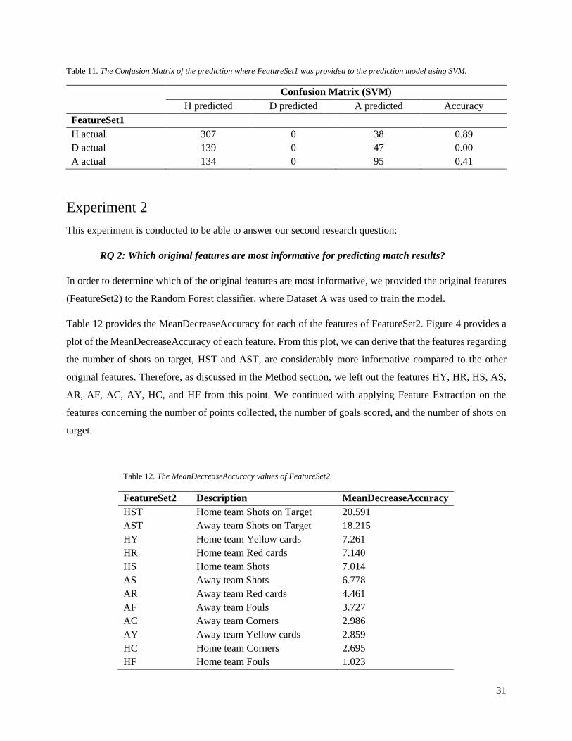
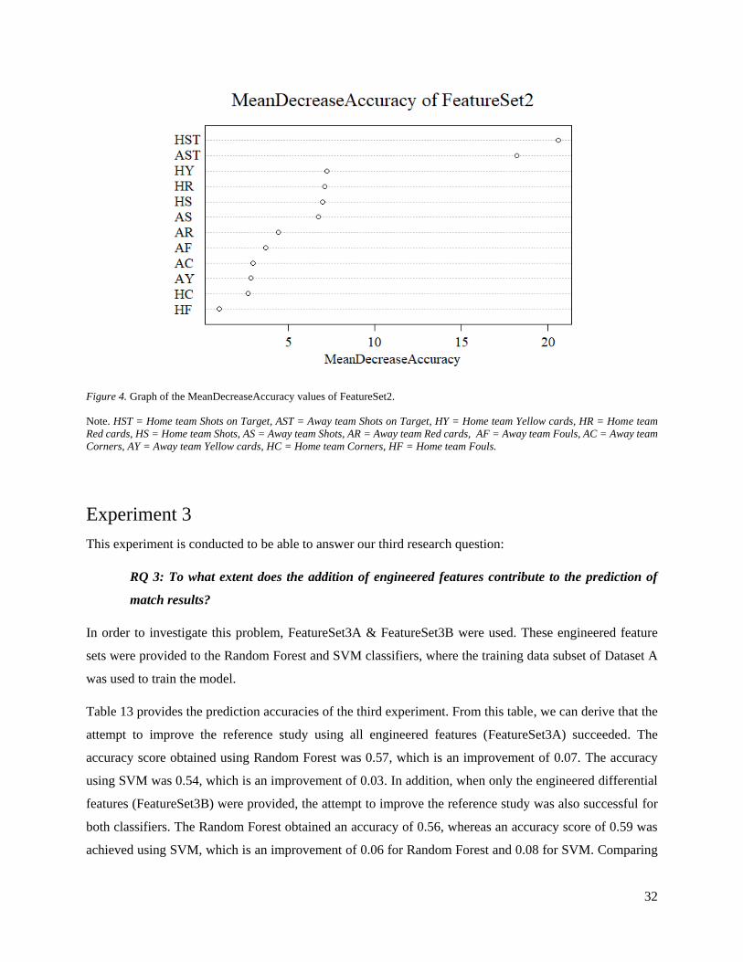
Table 12 provides the MeanDecreaseAccuracy for each of the features of FeatureSet2. Figure 4 provides a

plot of the MeanDecreaseAccuracy of each feature. From this plot, we can derive that the features regarding

the number of shots on target, HST and AST, are considerably more informative compared to the other

original features. Therefore, as discussed in the Method section, we left out the features HY, HR, HS, AS,

AR, AF, AC, AY, HC, and HF from this point. We continued with applying Feature Extraction on the

features concerning the number of points collected, the number of goals scored, and the number of shots on

target.

Table 12. The MeanDecreaseAccuracy values of FeatureSet2.

FeatureSet2 Description MeanDecreaseAccuracy

HST Home team Shots on Target 20.591

AST Away team Shots on Target 18.215

HY Home team Yellow cards 7.261

HR Home team Red cards 7.140

HS Home team Shots 7.014

AS Away team Shots 6.778

AR Away team Red cards 4.461

AF Away team Fouls 3.727

AC Away team Corners 2.986

AY Away team Yellow cards 2.859

HC Home team Corners 2.695

HF Home team Fouls 1.023

32

Figure 4. Graph of the MeanDecreaseAccuracy values of FeatureSet2.

Note. HST = Home team Shots on Target, AST = Away team Shots on Target, HY = Home team Yellow cards, HR = Home team

Red cards, HS = Home team Shots, AS = Away team Shots, AR = Away team Red cards, AF = Away team Fouls, AC = Away team

Corners, AY = Away team Yellow cards, HC = Home team Corners, HF = Home team Fouls.

Experiment 3

This experiment is conducted to be able to answer our third research question:

RQ 3: To what extent does the addition of engineered features contribute to the prediction of

match results?

In order to investigate this problem, FeatureSet3A & FeatureSet3B were used. These engineered feature

sets were provided to the Random Forest and SVM classifiers, where the training data subset of Dataset A

was used to train the model.

Table 13 provides the prediction accuracies of the third experiment. From this table, we can derive that the

attempt to improve the reference study using all engineered features (FeatureSet3A) succeeded. The

accuracy score obtained using Random Forest was 0.57, which is an improvement of 0.07. The accuracy

using SVM was 0.54, which is an improvement of 0.03. In addition, when only the engineered differential

features (FeatureSet3B) were provided, the attempt to improve the reference study was also successful for

both classifiers. The Random Forest obtained an accuracy of 0.56, whereas an accuracy score of 0.59 was

achieved using SVM, which is an improvement of 0.06 for Random Forest and 0.08 for SVM. Comparing

33

the results, we noted that Random Forest outperformed SVM regarding the improvement using

FeatureSet3A. In contrast, SVM outperformed Random Forest when FeatureSet3B was provided to the

prediction model. Overall, we can conclude that providing FeatureSet3B using SVM led to the best result,

which was 0.59 accuracy. The optimal values for the hyperparameters of the Random Forest models using

FeatureSet3A were 1000 trees to grow and minimum three examples required to split internal nodes. When

FeatureSet3B was applied, the optimal values were 500 for the number of trees to grow and the minimum

of five examples required to split internal nodes. The optimal values for the hyperparameters of the SVM

models that we found by tuning the prediction models were for both feature sets 0.1 for gamma and 1 for C.

Table 13. The prediction accuracies of FeatureSet3A and FeatureSet3B using Random Forest and SVM on Dataset A compared to

the study of Ulmer et al. (2013).

Classifier Dataset Prediction accuracy

Reference FeatureSet3A FeatureSet3B

Random Forest A 0.50 0.57 0.56

SVM A 0.51 0.54 0.59

From Table 14 and Table 15, which provides the confusion matrices of the four prediction tasks, we can

derive that, for both classifiers, FeatureSet3B predicted draws better compared to FeatureSet3A. Overall,

Random Forest performs better compared to SVM regarding the prediction of draws. In contrast to the

replication model using SVM (Table 11), draws were predicted by the improved prediction models using

SVM (Table 14), which is probably due to the application of class weights. Lastly, we observed that home

wins were predicted best by Random Forest with FeatureSet3A, draws by Random Forest with

FeatureSet3B, and away wins by SVM with FeatureSet3B.

Table 14. The Confusion Matrices of the predictions where FeatureSet3A and FeatureSet3B were provided to the prediction model

using Random Forest.

Confusion Matrix (Random Forest)

H predicted D predicted A predicted Accuracy

FeatureSet3A

H actual 296 13 36 0.86

D actual 115 14 57 0.08

A actual 87 21 121 0.53

FeatureSet3B

H actual 285 22 38 0.83

D actual 107 31 48 0.17

A actual 77 40 112 0.49

34

Table 15. The Confusion Matrices of the predictions where FeatureSet3A and FeatureSet3B were provided to the prediction model

using SVM.

Confusion Matrix (SVM)

H predicted D predicted A predicted Accuracy

FeatureSet3A

H actual 313 1 31 0.91

D actual 137 6 43 0.03

A actual 131 4 94 0.41

FeatureSet3B

H actual 296 20 29 0.86

D actual 118 15 53 0.08

A actual 66 25 138 0.60

Experiment 4

The last experiment is conducted to be able to answer our fourth research question:

RQ 4: To what extent does the extension of the dataset contribute to the prediction of match

results?

In order to investigate this problem, we extended Dataset A in different manners into Dataset B, Dataset C,

and Dataset D. FeatureSet1, FeatureSet3A, and FeatureSet3B were provided to the SVM classifier, which

was applied on the training data of the extended datasets.

The results of the prediction tasks of experiment 4 are shown in Table 16, where the accuracy scores of the

feature sets using Dataset A were obtained in experiment 1 and 3. From this table, we can derive that all

engineered features together (FeatureSet3A) yielded better prediction results than the replication features

(FeatureSet1) and that the differential features (FeatureSet3B) perform best. FeatureSet1 and FeatureSet3B

obtained the highest prediction accuracy on Dataset B, whereas FeatureSet3A obtained the best result on

Dataset D. All feature sets improved the accuracy score by 0.01 using Dataset B compared to Dataset A.

The accuracy scores decreased after the size of the dataset was further extended, except when all the

engineered features (FeatureSet3A) were provided to the prediction model. Overall, we can conclude that

providing FeatureSet1 to one of the extended datasets, Dataset C or Dataset D, led to the lowest score and

a decrease in prediction accuracy. We achieved our best prediction result by providing FeatureSet3B to

Dataset B. This resulted in an accuracy of 0.60, which is an improvement of 0.09 compared to the accuracy

that Ulmer et al. (2013) obtained when they predicted the same subset of test data using SVM. The values

of the hyperparameters for the SVM models that we found to be optimal by tuning were for each of the

35

prediction models 0.1 for gamma and 1 for C. Except for the model using FeatureSet1 and Dataset C, where

10 yielded optimal for C.

Table 16. The prediction accuracies of FeatureSet1, FeatureSet3A, and FeatureSet3B using SVM on Dataset A, Dataset B, Dataset

C, and Dataset D.

Classifier Dataset Prediction accuracy

FeatureSet1 FeatureSet3A FeatureSet3B

SVM A 0.53 0.54 0.59

SVM B 0.54 0.55 0.60

SVM C 0.51 0.55 0.59

SVM D 0.51 0.57 0.58

The Confusion Matrix of the prediction where FeatureSet1 was provided to Dataset B, Dataset C, and

Dataset D is shown in Table 17. We can derive that FeatureSet1 predicted no draws. Additionally, we noted

that as the size of the dataset increased, more home wins were predicted, and more home wins were predicted

correctly as well. However, the accuracy of FeatureSet1 on Dataset C and Dataset D decreased, which is

due to the fact that the number of correctly predicted away wins decreased.

Table 17. The Confusion Matrices of the predictions where FeatureSet1 was provided to the prediction model using Dataset B,

Dataset C, and Dataset D.

Confusion Matrix (FeatureSet1)

H predicted D predicted A predicted Accuracy

Dataset B

H actual 315 0 30 0.91

D actual 146 0 40 0.00

A actual 134 0 95 0.41

Dataset C

H actual 319 0 26 0.92

D actual 154 0 32 0.00

A actual 162 0 67 0.29

Dataset D

H actual 323 0 22 0.94

D actual 155 0 31 0.00

A actual 164 0 65 0.28

Table 18 provides the Confusion Matrix of the prediction model where FeatureSet3A was used. We can

derive that as the size of the dataset increased, the number of predicted home wins decreased, whereas the

number of predicted draws and away wins increased. FeatureSet3A obtained the highest accuracy using

Dataset D, where most of the advantage was gained by predicting more away wins correctly.

36

Table 18. The Confusion Matrices of the predictions where FeatureSet3A was provided to the prediction model using Dataset B,

Dataset C, and Dataset D.

Confusion Matrix (FeatureSet3A)

H predicted D predicted A predicted Accuracy

Dataset B

H actual 306 4 35 0.89

D actual 136 7 43 0.04

A actual 119 8 102 0.45

Dataset C

H actual 295 15 35 0.86

D actual 123 15 48 0.08

A actual 106 13 110 0.48

Dataset D

H actual 294 12 39 0.85

D actual 119 18 49 0.10

A actual 91 16 122 0.53

Table 19 shows the Confusion Matrix of the prediction results of FeatureSet3B using the three different

datasets. We observed that FeatureSet3B predicted more draws compared to the other feature sets.

Furthermore, FeatureSet3B correctly predicted away wins considerably more relative to FeatureSet1 and

FeatureSet3A.

Table 19. The Confusion Matrices of the predictions where FeatureSet3B was provided to the prediction model using Dataset B,

Dataset C, and Dataset D.

Confusion Matrix (FeatureSet3B)

H predicted D predicted A predicted Accuracy

Dataset B

H actual 296 19 30 0.86

D actual 117 15 54 0.08

A actual 65 16 148 0.65

Dataset C

H actual 287 24 34 0.83

D actual 101 20 65 0.11

A actual 61 28 140 0.61

Dataset D

H actual 284 27 34 0.82

D actual 97 18 71 0.10

A actual 57 31 141 0.62

Considering Table 17, Table 18, and Table 19, we can derive that increasing the amount of training data

(Dataset D) using FeatureSet1 had a positive effect on the prediction of home wins, which obtained an

37

accuracy of 0.94. The highest accuracy in regard to the prediction of draws was obtained by FeatureSet3B

using Dataset C, which was 0.11. FeatureSet3B using Dataset B yielded the highest accuracy regarding the

prediction of away wins. Overall, we can conclude that the use of larger datasets leads to the prediction of

fewer home wins, but more draws and away wins.

38

Discussion, Conclusion & Future Work

In this chapter, the results of the experiments are discussed in more detail. Subsequently, we answer the

research questions and the problem statement. Finally, recommendations for future work are suggested.

Discussion

The main goal of this study was to improve upon the prediction results of Ulmer et al. (2013) by using a

bigger dataset. An additional goal was to develop and evaluate novel features to enhance the prediction

accuracy. As validation for the results of this study, we succeeded in constructing replications of the

prediction models of Ulmer et al. (2013) using Random Forest and SVM. In our second experiment, we

determined that the original features regarding shots on target are most informative for predicting soccer

match results. Furthermore, the results showed that corners have a limited amount of predictive value, which

is contradictory to the study of Baboota and Kaur (2018) as they decided to include the original features

regarding corners in their feature extraction process. We decided to develop our engineered features based

on the number of shots on target of teams as well as based on the number of points collected and the number

of goals scored by teams.

In order to improve upon the accuracy that Ulmer et al. (2013) obtained, we provided our engineered features

to the model using the same classifiers and the same dataset. The highest accuracy they obtained was 0.51

using SVM, whereas our prediction model achieved an accuracy of 0.59 using the set of differential features.

This improvement is due to the development of features with more predictive ability regarding soccer match

results compared to the less advanced features that Ulmer et al. (2013) created. Subsequently, we provided

the same sets of engineered features to three different datasets. These datasets were extended in size relative

to the one Ulmer et al. (2013) used in their study, namely season-based extended, division-based extended,

and both season and division-based extended. The predictions of our model on the season-based extended

dataset using the differential feature set demonstrated a minor improvement. This resulted in the best

prediction result obtained in this study, which was an accuracy score of 0.60. However, the prediction ability

of our model decreased using the division-based extended dataset and both season and division-based

extended dataset. An explanation could be that the Premier League consists of less variation in terms of

team formation. The top teams of the Premier League rarely relegate to a lower division. Therefore, the

matches of these top teams are less difficult to predict as they win most of their matches. Only three teams

change in the formation of the Premier League each season, whereas in the Championship, League One,

and League Two change six, seven, and six teams, respectively. These irregularities probably negatively

affect the prediction of the soccer match results.

39

In order to put this study in context, we have to consider our results relative to those of Baboota and Kaur

(2018) as their study is currently state-of-the-art. They predicted the matches of the 2014/15 season and the

2015/16 season of the Premier League using a prediction model which was trained on data from the 2005/06

season until the 2015/16 season. Their prediction model using the classifier Random Forest obtained an

accuracy of 0.57, which is equal to the prediction accuracy of our Random Forest model. In contrast, their

prediction model using the classifier SVM performed worse with an accuracy score of 0.55, whereas we

obtained our best prediction performance using SVM which resulted in an accuracy score of 0.59. Moreover,

we achieved a prediction accuracy of 0.60 on the test set using the training subset that was extended by four

additional Premier League seasons. However, despite these accuracy scores improved upon the accuracy

scores of Baboota and Kaur (2018), it is important to remark that it is uncertain to what extent the

comparison of accuracy scores is reliable due to the seasonal effects.

Conclusion

In this study, we addressed the following overarching question: To what extent can we improve upon the

prediction results of Ulmer et al. (2013)? To be able to answer this problem statement, we formulated four

research questions. This section describes the answers to the research questions and concludes with the

answer to the problem statement.

RQ 1: To what extent can we replicate the study of Ulmer et al. (2013)?

In order to be able to validate the improvement of the prediction results of Ulmer et al. (2013), we first

replicated their prediction models. The obtained accuracy using Random Forest was equal, whereas there

was a minor difference in accuracy of 0.02 using SVM. Nevertheless, we considered our prediction model

as a successful replication.

Therefore, our answer to the first research question reads as follows:

Providing FeatureSet1 to the prediction model using the Random Forest classifier resulted in an accuracy

of 0.50, which is equal to the accuracy that Ulmer et al. (2013) obtained. Providing FeatureSet1 to the

prediction model using the SVM classifier resulted in an accuracy of 0.53, which is a difference of 0.02

compared to the accuracy that Ulmer et al. (2013) obtained.

RQ 2: Which original features are most informative for predicting match results?

We determined which features are most informative when predicting match results in English professional

soccer by providing the original features (FeatureSet2) to the Random Forest classifier, where Dataset A

was used to train the model. The results of this experiment demonstrated that the features regarding the

40

number of shots on target, which are HST and AST, are considerably more informative compared to the

other original features. Shots on target are in fact the match events which are closest to an actual goal scored.

Therefore, the results of this experiment were perfectly in line with our expectations and the findings of

Baboota and Kaur (2018). They also included the shots on target features from the original dataset after a

careful analysis.

Hence, our answer to the first research question reads as follows:

For both the home team and the away team, the feature regarding the number of shots on target is most

informative when predicting match results.

RQ 3: To what extent does the addition of engineered features contribute to the prediction of

match results?

We used two different sets of features in order to investigate this problem, namely FeatureSet3A and

FeatureSet3B. FeatureSet3A consists of all the engineered features, where FeatureSet3B consists of only

the differential features that were engineered. Both sets of features improved the accuracy of the prediction

models for both classifiers. Further, Random Forest achieved the highest accuracy when FeatureSet3A was

provided, whereas SVM obtained the highest accuracy with FeatureSet3B. The difference between these

models is the predictions of away wins. Random Forest provided with FeatureSet3A obtained prediction

accuracies of 0.86, 0.08, and 0.53 for the classes H, D, and A, respectively. SVM provided with

FeatureSet3B obtained prediction accuracies of 0.86, 0.08, and 0.60 for the classes H, D, and A, respectively.

Thus, the difference in accuracy is the result of the ability to predict away wins correctly. Regarding the

prediction model where FeatureSet3A was provided to the SVM classifier, we were probably overfitting

our data. The accuracy increased only marginally relative to the replicated model, whereas the number of

included features increased from six to 66. Furthermore, SVM provided with FeatureSet3B, which is a

subset of FeatureSet3A, improved the accuracy considerably.

Lastly, contradictory to the replicated SVM model, our improved SVM model predicted draws. We added

class weights to the prediction model in order to increase the likelihood that draws are predicted. However,

whether the class weights are fully responsible for the expected result is uncertain.

To conclude with, our answer to the second research question reads as follows:

Providing FeatureSet3A to the prediction model using the Random Forest classifier resulted in an accuracy

of 0.57, which is an improvement of 0.07 compared to the accuracy that Ulmer et al. (2013) obtained.

Providing FeatureSet3B to the prediction model using the SVM classifier resulted in an accuracy of 0.59,

which is an improvement of 0.08 compared to the accuracy that Ulmer et al. (2013) obtained.

41

RQ 4: To what extent does the extension of the dataset contribute to the prediction of match

results?

In order to answer this research question, we extended Dataset A season-based (Dataset B), division-based

(Dataset C), and both season and division-based (Dataset D). We provided FeatureSet1, FeatureSet3A, and

FeatureSet3B to the prediction model using the training data of the extended datasets and the classifier

SVM. The extension of the dataset resulted in a decrease in accuracy regarding the prediction of home wins,

except for FeatureSet1. The accuracy of the prediction of draws increased marginally as the size of the

datasets extended. The extension of the dataset had a negative effect on the prediction accuracy of away

wins using FeatureSet1 and a positive effect using FeatureSet3A.

Considering the overall accuracy scores of the prediction models, we can conclude that the extension of the

dataset into Dataset B yielded marginally better prediction results relative to the accuracy scores obtained

on Dataset A in experiment 3. However, only one out of six accuracy scores which we obtained by providing

the feature sets to our model using Dataset C and Dataset D achieved an increase. These results indicate that

that extending the dataset division-based does not improve the prediction ability, which is probably due to

the fact that the divisions differ from each other in predictability.

Hence, our answer to the fourth research question reads as follows:

Providing the feature sets to the prediction model using the dataset which was season-based extended

resulted in a marginal improvement of 0.01 compared to the accuracy that we obtained using the same size

of the dataset as Ulmer et al. (2013). Providing the feature sets to the prediction model using the datasets

which were division-based extended and both season and division-based extended resulted in a decrease

compared to the accuracy that we obtained using the same size of the dataset as Ulmer et al. (2013).

To what extent can we improve upon the prediction results of Ulmer et al. (2013)?

To be able to answer this problem statement, we summarize the answers to the four research questions. Our

answer to the problem statement reads as follows:

We succeeded in replicating the study of Ulmer et al. (2013), which validates the results of our study.

Additionally, we determined that the original features regarding shots on target are most informative.

Furthermore, we created feature sets consisting of engineered features, which outperformed the prediction

results of Ulmer et al. (2013) using the same size of the dataset. Particularly, using FeatureSet3B and Dataset

A, we achieved an accuracy of 0.59, which is an improvement of 0.08. The extension of the dataset season-

based resulted in a marginal improvement. Using FeatureSet3B and Dataset B, we achieved an accuracy of

42

0.60, which is the best prediction result of this study. Finally, extending the size of the dataset division-

based and both season and division-based did not contribute to the prediction of match results.

Future Work

First of all, one of the main difficulties of predicting soccer match results is the randomness of the data,

which is also addressed by Ulmer et al. (2013). For instance, the randomness of the data relates to the

unbalanced classes H, D, and A. We attempted to counter this difficulty by applying class weights. However,

it is uncertain whether these class weights resulted in more correct predictions. This required additional

experiments, which we did not engage in this study. Furthermore, randomness in the performance of

different teams, which can be seen as outliers, makes predicting match results correctly difficult. Despite

increasing the amount of data normally often reduces the influence of outliers and improves the prediction

ability, the results of our fourth experiment demonstrated the opposite. Another consequence of the

randomness in performance is the difficulty of detecting overfitting on the data regarding the prediction of

soccer match results. This is due to the fact that the soccer matches in the test set could be unrepresentative

for the results of the matches in the training set.

Additionally, the manner in which some of the engineered features were created could be a point of

improvement for this study. To start with, the features regarding the strength of teams and the ranking of

teams were engineered based on data over the period of the 2002/03 season until the 2011/12 season.

Therefore, these features represent the strength of teams over this period of 10 seasons. In contrast, all other

engineered features were created season-based for the purpose of predicting match results for each season

separately. However, the dataset used in this study did not contain data about league standings per season,

and calculating the team strengths for each of the 64 competitions separate would have been time-

consuming. Another issue of feature engineering that we encountered was that the cumulative engineered

features are of less influence in the first part of the season because the differences between teams are not

evident yet. Lastly, we focused on the match statistics about the number of points collected, the number of

goals scored, and the number of shots on target. However, we did not engineer new features based on the

number of goals conceded. Furthermore, we did not engineer new features based on previous matches

between two specific teams due to the words of Constantinou et al. (2012) who stated that historical

performances of two teams are not representative for their current strength.

To mention a shortcoming of this study, we engineered the form and weighted form features by using the

same number of previous matches as Ulmer et al. (2013) showed to be optimal in their study. In this case,

the previous 7 matches for the Random Forest classifier and the previous 4 matches when SVM was applied.

Nevertheless, to ensure that the optimal number of previous matches for our study is used, this could be

43

tested by an additional experiment. For instance, replicating this study with a varying number of previous

matches in the range of 2 to 8 to calculate the form.

As previously stated, in experiment 4 we extended the size of the dataset. We chose to use the same subset

as test data for all our prediction models to ensure reliable comparisons. Because of this, we were forced to

use the training data of seasons that lie in the future relative to the test set. Therefore, the prediction models

where Dataset B and Dataset D were used are in fact not prediction tasks. Hence, we suggest repeating this

study using the two most recent seasons as the test set and the previous seasons as training data in order to

determine whether this affected the results of our investigation. Additionally, comparing our accuracy scores

relative to the accuracy scores of Baboota and Kaur (2018) implies that we also improved upon their

prediction results. However, we recommend applying our developed prediction model to the same subsets

of training data and testing data as they used. Based on the results of that experiment we could conclude to

whether we also improved upon the prediction results of the study of Baboota and Kaur (2018), which is

the current state-of-the-art.

As a final point, in the Introduction chapter of this thesis we stated that although our study focusses on

English professional soccer, our developed prediction model is easily applicable to other European top

soccer competitions. Hence, we wish to apply our prediction model to other competitions to explore the

extent to which the match results of these competitions can be predicted correctly.

44

References

Aoki, R., Assuncao, R. M., & Vaz de Melo, P. O. (2017). Luck is hard to beat: The difficulty of

sports prediction. In Proceedings of the 23rd ACM SIGKDD International Conference on Knowledge

Discovery and Data Mining (pp. 1367-1376). ACM.

Baboota, R., & Kaur, H. (2018). Predictive analysis and modelling football results using machine

learning approach for Premier League. International Journal of Forecasting.

Breiman, L. (2001). Random forests. Machine learning, 45(1), 5-32.

Constantinou, A. C., Fenton, N. E., & Neil, M. (2012). pi-football: A Bayesian network model for

forecasting Association Football match outcomes. Knowledge-Based Systems, 36, 322-339.

Dowle, M., & Srinivasan, A. (2017). data.table: Extension of `data.frame`. R package version

1.10.4-3. https://CRAN.R-project.org/package=data.table

Football-Data. (2018). Football-Data.co.uk. European Football Results and Betting Odds [database

file]. Retrieved from http://www.football-data.co.uk/englandm.php

Gomes, J., Portela, F., & Santos, M. F. (2015). Decision Support System for predicting Football

Game result. In Computers-19th International Conference on Circuits, Systems, Communications and

Computers-Intelligent Systems and Applications Special Sessions. Series (Vol. 32, pp. 348-353).

Holmes, E. (2013). fbRanks: Association Football (Soccer) Ranking via Poisson Regression. R

package version 2.0. https://CRAN.R-project.org/package=fbRanks

Jones, M. B. (2018). Differences in home advantage between sports. Psychology of Sport and

Exercise, 34, 61-69.

Kuhn, M. (2008). Caret package. Journal of Statistical Software, 28(5)

Liaw, A., & Wiener, M. (2002). Classification and Regression by randomForest. R News 2(3), 18-

-22.

Meyer, D., Dimitriadou, E., Hornik, K., Weingessel, A., & Leisch, F. (2017). e1071: Misc Functions

of the Department of Statistics, Probability Theory Group (Formerly: E1071), TU Wien. R package version

1.6-8. https://CRAN.R-project.org/package=e1071

Pollard, R. (1986). Home advantage in soccer: A retrospective analysis. Journal of sports

sciences, 4(3), 237-248.

45

R Core Team (2017). R: A language and environment for statistical computing. R Foundation for

Statistical Computing, Vienna, Austria. URL https://www.R-project.org/.

Razali, N., Mustapha, A., Utama, S., & Din, R. (2018). A Review on Football Match Outcome

Prediction using Bayesian Networks. In Journal of Physics: Conference Series (Vol. 1020, No. 1, p.

012004). IOP Publishing.

Razali, N., Mustapha, A., Yatim, F. A., & Ab Aziz, R. (2017). Predicting Football Matches Results

using Bayesian Networks for Premier League (EPL). In IOP Conference Series: Materials Science and

Engineering (Vol. 226, No. 1, p. 012099). IOP Publishing.

Rossi, A., Pappalardo, L., Cintia, P., Iaia, M., Fernández, J., & Medina, D. (2017). Effective injury

prediction in professional soccer with GPS data and machine learning. arXiv preprint arXiv:1705.08079.

RStudio Team (2016). RStudio: Integrated Development for R. RStudio, Inc., Boston, MA URL

http://www.rstudio.com/.

Snyder, J. A. L. (2013). What Actually Wins Soccer Matches: Prediction of the 2011-2012 Premier

League for Fun and Profit (Doctoral dissertation, Master’s thesis).

Tax, N., & Joustra, Y. (2015). Predicting the Dutch football competition using public data: A

machine learning approach. Transactions on Knowledge and Data Engineering, 10(10), 1-13.

Ulmer, B., Fernandez, M., & Peterson, M. (2013). Predicting Soccer Match Results in the Premier

League (Doctoral dissertation, Doctoral dissertation, Ph. D. dissertation, Stanford).

Vroonen, R., Decroos, T., Van Haaren, J., & Davis, J. (2017). Predicting the potential of

professional soccer players. In Machine Learning and Data Mining for Sports Analytics ECML/PKDD 2017

workshop.

Wang, Q., Zhu, H., Hu, W., Shen, Z., & Yao, Y. (2015). Discerning tactical patterns for professional

soccer teams: an enhanced topic model with applications. In Proceedings of the 21th ACM SIGKDD

International Conference on Knowledge Discovery and Data Mining (pp. 2197-2206). ACM.

Wickham, H., & Henry, L. (2017). tidyr: Easily Tidy Data with 'spread()' and 'gather()' Functions.

R package version 0.7.2. https://CRAN.R-project.org/package=tidyr

Wickham, H., Francois, R., Henry, L., & Müller, K. (2017). dplyr: A Grammar of Data

Manipulation. R package version 0.7.4. https://CRAN.R-project.org/package=dplyr

46

Zeileis, A., & Grothendieck, G. (2005). zoo: S3 Infrastructure for Regular and Irregular Time Series.

Journal of Statistical Software, 14(6), 1-27. doi:10.18637/jss.v014.i06

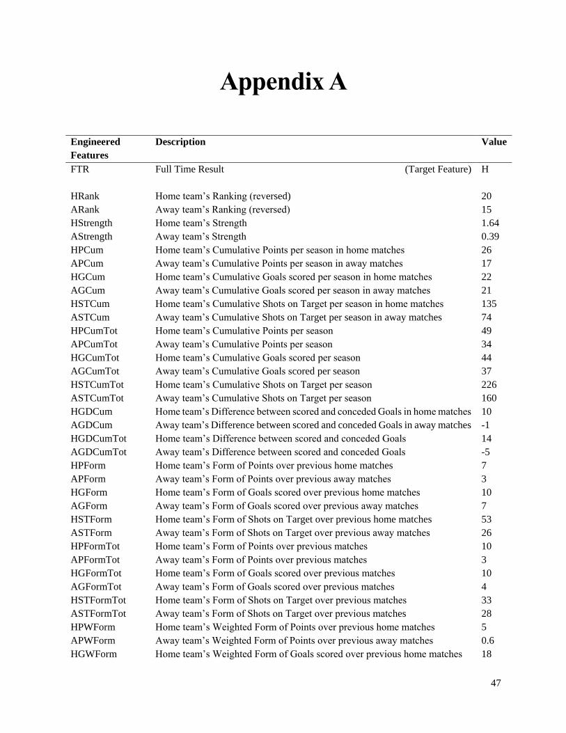
47

Appendix A

Engineered

Features

Description Value

FTR

Full Time Result (Target Feature) H

HRank Home team’s Ranking (reversed) 20

ARank Away team’s Ranking (reversed) 15

HStrength Home team’s Strength 1.64

AStrength Away team’s Strength 0.39

HPCum Home team’s Cumulative Points per season in home matches 26

APCum Away team’s Cumulative Points per season in away matches 17

HGCum Home team’s Cumulative Goals scored per season in home matches 22

AGCum Away team’s Cumulative Goals scored per season in away matches 21

HSTCum Home team’s Cumulative Shots on Target per season in home matches 135

ASTCum Away team’s Cumulative Shots on Target per season in away matches 74

HPCumTot Home team’s Cumulative Points per season 49

APCumTot Away team’s Cumulative Points per season 34

HGCumTot Home team’s Cumulative Goals scored per season 44

AGCumTot Away team’s Cumulative Goals scored per season 37

HSTCumTot Home team’s Cumulative Shots on Target per season 226

ASTCumTot Away team’s Cumulative Shots on Target per season 160

HGDCum Home team’s Difference between scored and conceded Goals in home matches 10

AGDCum Away team’s Difference between scored and conceded Goals in away matches -1

HGDCumTot Home team’s Difference between scored and conceded Goals 14

AGDCumTot Away team’s Difference between scored and conceded Goals -5

HPForm Home team’s Form of Points over previous home matches 7

APForm Away team’s Form of Points over previous away matches 3

HGForm Home team’s Form of Goals scored over previous home matches 10

AGForm Away team’s Form of Goals scored over previous away matches 7

HSTForm Home team’s Form of Shots on Target over previous home matches 53

ASTForm Away team’s Form of Shots on Target over previous away matches 26

HPFormTot Home team’s Form of Points over previous matches 10

APFormTot Away team’s Form of Points over previous matches 3

HGFormTot Home team’s Form of Goals scored over previous matches 10

AGFormTot Away team’s Form of Goals scored over previous matches 4

HSTFormTot Home team’s Form of Shots on Target over previous matches 33

ASTFormTot Away team’s Form of Shots on Target over previous matches 28

HPWForm Home team’s Weighted Form of Points over previous home matches 5

APWForm Away team’s Weighted Form of Points over previous away matches 0.6

HGWForm Home team’s Weighted Form of Goals scored over previous home matches 18

48

AGWForm Away team’s Weighted Form of Goals scored over previous away matches 26.4

HSTWForm Home team’s Weighted Form of Shots on Target over previous home matches 23.8

ASTWForm Away team’s Weighted Form of Shots on Target over previous away matches 12.6

HPWFormTot Home team’s Weighted Form of Points over previous matches 6.4

APWFormTot Away team’s Weighted Form of Points over previous matches 1.2

HGWFormTot Home team’s Weighted Form of Goals scored over previous matches 6.2

AGWFormTot Away team’s Weighted Form of Goals scored over previous matches 3.2

HSTWFormTot Home team’s Weighted Form of Shots on Target over previous matches 18.8

ASTWFormTot Away team’s Weighted Form of Shots on Target over previous matches 19

RankDiff Difference between HRank and ARank 5

StrengthDiff Difference between HStrength and AStrength 1.25

PCumDiff Difference between HPCum and APCum 9

GCumDiff Difference between HGCum and AGCum 1

STCumDiff Difference between HSTCum and ASTCum 61

PCumTotDiff Difference between HPCumTot and APCumTot 15

GCumTotDiff Difference between HGCumTot and AGCumTot 7

STCumTotDiff Difference between HSTCumTot and ASTCumTot 66

GDCumDiff Difference between HGDCum and AGDCum 11

GDCumTotDiff Difference between HGDCumTot and AGDCumTot 19

PFormDiff Difference between HPForm and APForm 4

GFormDiff Difference between HGForm and AGForm 3

STFormDiff Difference between HSTForm and ASTForm 27

PFormTotDiff Difference between HPFormTot and APFormTot 7

GFormTotDiff Difference between HGFormTot and AGFormTot 6

STFormTotDiff Difference between HSTFormTot and ASTFormTot 5

PWFormDiff Difference between HPWForm and APWForm 4.4

GWFormDiff Difference between HGWForm and AGWForm -8.4

STWFormDiff Difference between HSTWForm and ASTWForm 11.2

PWFormTotDiff Difference between HPWForm and APWForm 5.2

GWFormTotDiff Difference between HGWForm and AGWForm 3

STWFormTotDiff Difference between HSTWForm and ASTWForm -0.2