improving test of theories in positing interaction

Improving Tests of Theories Positing Interaction

William D. Berry Florida State University

Matt Golder Pennsylvania State University

Daniel Milton Brigham Young University

It is well established that all interactions are symmetric: when the effect of X on Y is conditional on the value of Z,the effect of Z must be conditional on the value of X. Yet the typical practice when testing an interactive theory is to(1) view one variable, Z, as the conditioning variable, (2) offer a hypothesis about how the marginal effect of theother variable, X, is conditional on the value of Z, and (3) construct a marginal effect plot for X to test the theory.We show that the failure to make additional predictions about how the effect of Z varies with the value of X, and toevaluate them with a second marginal effect plot, means that scholars often ignore evidence that can be extremelyvaluable for testing their theory. As a result, they either understate or, more worryingly, overstate the support fortheir theories.

Since many political theories assert that theeffects of variables vary depending on the social,political, economic, or strategic context, models

specifying interaction among variables are ubiquitousacross all subfields of political science.1,2 A conse-quence is that conditional hypotheses such as ‘‘X hasa positive effect on Y that gets stronger as Z increases’’are extremely common. It is well established thatinteractive statistical models containing multiplica-tive terms, such as XZ, are appropriate for evaluatingsuch conditional hypotheses (Aiken and West 1991;Clark, Gilligan, and Golder 2006; Friedrich 1982;Wright 1976).3 A number of authors in recent yearshave offered valuable advice on how to improveresearch testing theories positing interaction byproperly specifying the expected conditionality in astatistical model and effectively presenting and inter-preting the results (Braumoeller 2004; Brambor,Clark, and Golder 2006; Kam and Franzese 2007).However, even researchers following this advice oftenignore valuable empirical evidence that can be easilyderived from their estimated model and as a result,

fail to assess all of the predictions generated by theirtheory. The result is that many researchers either un-derstate, or, more worryingly, overstate the empiricalsupport for their conditional theories.

The inadequacy of many empirical tests of condi-tional theories can be traced to the tendency ofscholars positing interaction between two variablesto conceive of these variables as having different roleswithin the theory. One variable, Z, is typically viewedas the ‘‘conditioning variable,’’ the role of which isto modify the impact of the other variable, X, onthe dependent variable, Y. Certainly, when X and Zinteract, it is reasonable to conceive of Z as condi-tioning the effect of X on Y. However, it makes littlesense to view X and Z as having fundamentallydifferent theoretical roles by designating one of thevariables as a ‘‘conditioning variable’’ and the otheras not. This is because, logically, all interactions aresymmetric (Brambor, Clark, and Golder 2006; Kamand Franzese 2007). In other words, if Z modifies theeffect of X on Y, then X must modify the effect of Z onY. Some might view conceiving of one variable as the

The Journal of Politics, Vol. 74, No. 3, July 2012, Pp. 653–671 doi:10.1017/S0022381612000199

� Southern Political Science Association, 2012 ISSN 0022-3816

1The data and all computer code necessary to replicate our results are publicly available at the authors’ web sites: http://mailer.fsu.edu/;wberry/garnet-wberry/ (for Berry), https://files.nyu.edu/mrg217/public/ (for Golder), or http://myweb.fsu.edu/djm07g/index.html(for Milton). Stata 11 was used for all statistical analyses.

2In a systematic examination of three leading journals (American Journal of Political Science, American Political Science Review, andJournal of Politics) from 1996 to 2001, Kam and Franzese (2007, 7–8) find that fully 24% of articles employing ‘‘statistical methods’’tested theories predicting interaction.

3We treat the terms ‘‘theory positing interaction,’’ ‘‘interactive theory,’’ and ‘‘conditional theory’’ as synonymous.

653

‘‘conditioning variable’’ and failing to acknowledgethe symmetry of interaction as merely a semanticproblem. We demonstrate, however, that this practicecan have pernicious consequences, leading research-ers to ignore empirical evidence relevant for testingtheir theory.

In a much-cited 2006 article, Brambor, Clark,and Golder [hereafter BCG] demonstrate that polit-ical scientists can greatly increase their ability toimpart substantively meaningful information frominteractive models by using parameter estimates toconstruct a marginal effect plot for an independentvariable, i.e., a graph that shows how the marginaleffect of the variable varies with the value of anothervariable. Scholars have responded in large numbers toBCG’s call to incorporate marginal effect plots intotheir analyses. Indeed, within three years of the ap-pearance of BCG’s article, at least 44 publishedpapers presented such plots.4 This has dramaticallyimproved the interpretation of statistical resultsfrom interactive models in the literature. Ironically,however, BCG’s article may have inadvertentlyencouraged its readers to make the mistake of viewingone variable as the ‘‘conditioning variable.’’ AlthoughBCG (2006, note 9) correctly observe that interactivemodels are symmetric and that the marginal effect ofeach independent variable is a ‘‘meaningful’’ quantityof interest, they go on to imply that analysts mightreasonably establish one of these quantities as thefocus of theoretical interest and produce only onemarginal effect plot. Indeed, of the 44 papers weidentified that present marginal effect plots to evaluatea theory positing interaction, 39 (89%) present only asingle plot, showing how the estimated effect of onevariable varies with the other.

We accept as a fundamental principle that scholarsestimating a statistical model should use the estimationresults to assess as many of the theory’s implications aspossible. We show that for those testing theoriespositing interaction between two independent varia-bles, this often means deriving and testing predictionsabout how the marginal effect of each independentvariable varies with the value of the other not all ofwhich can be evaluated by inspecting a single marginaleffect plot. It is important to note that we are notsuggesting that researchers testing a hypothesis abouthow the marginal effect of X varies with Z should‘‘manufacture’’ a second hypothesis about how themarginal effect of Z varies with X when their theory

generates no predictions beyond those already in-corporated in the first hypothesis. We are simplyobserving that many conditional theories proposedby political scientists generate more predictions thancan be tested with a single marginal effect plot, andthat in this situation, when the researcher limitsconsideration to a single plot, she subjects her theoryto a weaker test than is possible given the dataavailable.

In the next section, we consider the implicationsof the inherent symmetry of interactive models fortheory testing in more detail. In particular, wedemonstrate why it can be dangerous for a re-searcher with a conditional theory to limit consid-eration to predictions that can be evaluated with asingle marginal effect plot. The basic insight is thatany observed relationship between Z and the mar-ginal effect of X is always consistent with a widevariety of ways in which the marginal effect of Zvaries with X, some of which may be inconsistentwith the underlying conditional theory. This meansthat proposing a hypothesis about how the effect ofX varies with Z and assessing it by examining justa marginal effect plot for X often constitutes a weak testof the conditional theory underlying the hypothesis.Supplementing this hypothesis with a second oneabout how the effect of Z varies with X that can beevaluated by inspecting a marginal effect plot for Zcan dramatically narrow the range of relationshipsthat are consistent with one’s underlying theory,thereby strengthening the empirical test.

We then turn to practical advice on derivingand testing hypotheses from conditional theories. Inparticular, we discuss issues that arise when evalu-ating empirical evidence in favor of, or against,conditional theories by examining several prototyp-ical sets of results one might get when estimating aninteractive model. Many of these issues have notbeen adequately addressed in the existing literature,leaving some readers uncertain as to how to evaluatethe level of empirical support for conditional theo-ries. Next, we illustrate our central points by rep-licating two of the numerous published studies thatseek to test a conditional theory but that present amarginal effect plot for only one of the two variablespredicted to interact. In one replication, construct-ing a second marginal effect plot reveals additionalsupport for the researcher’s theory. In the other, asecond plot reveals evidence contrary to the analyst’stheory. Throughout the article, we offer advice onhow to maximize the information portrayed inmarginal effect plots, and before concluding, wesummarize our recommendations.

4As of January 2009, 44 published articles in the ISI Web ofKnowledge database cite BCG’s (2006) article and present at leastone marginal effect plot.

654 william d. berry et al.

Implications of the Symmetry ofInteraction for Theory Testing

Suppose we have a conditional theory in which X andZ interact in influencing some continuous dependentvariable, Y, such that the effects of X and Z can becaptured with the following linear-interactive model:5

Y ¼ b0 þ bX X þ bZ Z þ bXZ XZ þ e: ð1Þ

This model—involving a single product, or multi-plicative, term—is the most common specification ofinteraction in political science. In this model, themarginal effect of X, @Y/@X, is given by:

@Y

@X¼ bX þ bXZ Z: ð2Þ

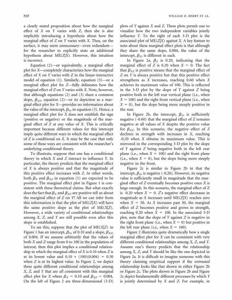
As equation (2) clearly indicates, unless the coeffi-cient for the product term, bXZ, is zero, the marginaleffect of X is conditional on the value of Z.6 Toemphasize this conditionality in what follows, wedenote the marginal effect of X as ME(X|Z). In turn,we let ME(X|Z 5 z) denote the marginal effect of Xon Y when Z equals the specific value z. The marginaleffect plot for X in Figure 1 depicts the relationshipbetween ME(X|Z) and Z in equation (2) when bX

and bXZ are both positive. The plot illustrates that (a)when Z 5 0, the marginal effect of X on Y is bX, and(b) due to the constant slope, bXZ, of equation (2),the marginal effect of X changes by bXZ for every unitincrease in Z.

Note that the interactive model specified inequation (1) is symmetric in X and Z. In other words,the fact that the marginal effect of X on Y is condi-tional on Z logically guarantees that the marginaleffect of Z on Y must be conditional on X. Indeed, themarginal effect of Z is given by:

MEðZjXÞ ¼ @Y

@Z¼ bZ þ bXZX: ð3Þ

This implies that the marginal effect of Z is bZ when X iszero and changes by bXZ for every unit increase in X.Thus, it is evident that the coefficient on the productterm, bXZ, indicates both the slope of the relationshipbetween ME(X|Z) and Z and the slope of the rela-tionship between ME(Z|X) and X. As such, we mustrecognize that Z conditions the effect of X on Y, and Xconditions the effect of Z on Y. It is this inherentsymmetry that makes it misleading for scholars todesignate X or Z as the conditioning variable and theother variable as the one being conditioned.7 We rec-ognize that in some settings it can be very tempting toconceive of one variable as the conditioning variable.For example, when one variable, X, is continuous andthe other, Z, is dichotomous, it seems natural to thinkin terms of the effect of X on Y being different in onecontext (Z 5 0) than in another (Z 5 1), therebyestablishing Z as the conditioning variable. However,the fact remains that the effect of the binary variable Zalso varies with X.

Although the inherent symmetry of interactionsis well-documented (Brambor, Clark, and Golder2006; Kam and Franzese 2007), the implications ofsuch symmetry for theory testing have been largelyoverlooked. Recall that the product-term coefficient,bXZ, in equation (1) indicates both the slope of therelationship between ME(X|Z) and Z and the slope ofthe relationship between ME(Z|X) and X. This impliesthat if a researcher with a conditional theory presents

FIGURE 1 A Plot of the Marginal Effect of X on Yagainst Z when bX and bXZ inequation (1) are Positive

5For simplicity, we assume that there are no other covariates inthe model. However, all claims in this article hold with anynumber of additional variables as long as none of them interactswith either X or Z. Although we focus on models with continuousdependent variables, our advice is equally applicable to modelswith limited dependent variables such as logit and probit.

6Note that the expression for @Y/@X in equation (2) implies thatthe marginal effect of X on Y is conditional on the value of Z butnot on the value of X. This property stems from the linearfunctional form for the interaction specified in equation (1). Ininteractive models with a nonlinear functional form, in contrast,the marginal effect of X on Y necessarily varies with both the valueof X and the value of Z (Brambor, Clark, and Golder 2006, 77).

7We should note that the inherent symmetry of interactions isnot the result of the particular linear-interactive specification thatwe use in equation (1); all interactive specifications are symmet-ric (Kam and Franzese 2007, 16).

improving tests of interactive theories 655

a clearly stated proposition about how the marginaleffect of X on Y varies with Z, then she is alsoimplicitly introducing a hypothesis about how themarginal effect of Z on Y varies with X. Thus, on thesurface, it may seem unnecessary—even redundant—for the researcher to explicitly state an additionalhypothesis about ME(Z|X). However, this intuitionis incorrect.

Equation (2)—or equivalently, a marginal effectplot for X—completely characterizes how the marginaleffect of X on Y varies with Z in the linear-interactivemodel of equation (1). Similarly, equation (3)—or amarginal effect plot for Z—fully delineates how themarginal effect of Z on Y varies with X. Note, however,that although equations (2) and (3) share a commonslope, bXZ, equation (2)—or its depiction as a mar-ginal effect plot for X—provides no information aboutthe value of the intercept, bZ, in equation (3). Hence, amarginal effect plot for X does not establish the sign(positive or negative) or the magnitude of the mar-ginal effect of Z at any value of X. This is criticallyimportant because different values for this interceptimply quite different ways in which the marginal effectof Z is conditional on X. It may be the case that onlysome of these ways are consistent with the researcher’sunderlying conditional theory.

To illustrate, suppose that one has a conditionaltheory in which X and Z interact to influence Y. Inparticular, the theory predicts that the marginal effectof X is always positive and that the magnitude ofthis positive effect increases with Z. In other words,both bX and bXZ in equation (1) are expected to bepositive. The marginal effect plot in Figure 1 is con-sistent with these theoretical claims. But what exactlydoes the fact that bX and bXZ are positive tell us aboutthe marginal effect of Z on Y? All we can infer fromthis information is that the plot of ME(Z|X) will havethe same positive slope as the plot of ME(X|Z).However, a wide variety of conditional relationshipsamong X, Z, and Y are still possible even after thisslope is established.

To see this, suppose that the plot of ME(X|Z) inFigure 1 has an intercept, bX, of 0.10 and a slope, bXZ,of 0.004. If we assume arbitrarily that the values ofboth X and Z range from 0 to 100 in the population ofinterest, then this plot implies a conditional relation-ship in which the marginal effect of X is 0.10 when Z isat its lowest value and 0.10 + (100)(0.004) 5 0.50when Z is at its highest value. In Figure 2, we depictthree quite different conditional relationships amongX, Z, and Y that are all consistent with this marginaleffect plot for X where bX 5 0.10 and bXZ 5 0.004.On the left of Figure 2 are three-dimensional (3-D)

plots of Y against X and Z. These plots permit one tovisualize how the two independent variables jointlyinfluence Y. To the right of each 3-D plot is theassociated plot of ME(Z|X) against X. A key feature tonote about these marginal effect plots is that althoughthey share the same slope, 0.004, the value of theintercept, bZ, is different in each.

In Figure 2a, bZ is 0.20, indicating that themarginal effect of Z is 0.20 when X 5 0. The factthat bXZ is positive means that the marginal effect ofZ on Y is always positive but that this positive effectstrengthens as X increases, reaching 0.60 when Xachieves its maximum value of 100. This is reflectedin the 3-D plot by the slope of Y against Z beingpositive both in the left rear vertical plane (i.e., whenX 5 100) and the right front vertical plane (i.e., whenX 5 0), but the slope being more steeply positive inthe rear.

In Figure 2b, the intercept, bZ, is sufficientlynegative (-0.60) that the marginal effect of Z remainsnegative at all values of X despite the positive valuefor bXZ. In this scenario, the negative effect of Zdeclines in strength with increases in X, reaching-0.20 when X obtains its maximum value. This ismirrored in the corresponding 3-D plot by the slopeof Y against Z being negative both in the left rearplane (i.e., when X 5 100) and the right front plane(i.e., when X 5 0), but the slope being more steeplynegative in the front.

Figure 2c is similar to Figure 2b in that theintercept, bZ, is negative (-0.20). However, its negativevalue is sufficiently small in magnitude that the mar-ginal effect of Z eventually becomes positive once X islarge enough. In this scenario, the marginal effect of Zis -0.20 when X 5 0. Z’s negative effect decreases inmagnitude as X increases until ME(Z|X) reaches zerowhen X 5 50. As X increases past 50, the marginaleffect of Z becomes positive and grows in strength,reaching 0.20 when X 5 100. In the associated 3-Dplot, note that the slope of Y against Z is negative inthe right front plane (i.e., when X 5 0) but positive inthe left rear plane (i.e., when X 5 100).

Figure 2 illustrates quite dramatically how a singlemarginal effect plot for X can be consistent with verydifferent conditional relationships among X, Z, and Y.Assume one’s theory predicts that the relationshipamong X, Z, and Y should be like the one depicted inFigure 2a. It is difficult to imagine someone with thistheory claiming empirical support if the estimatedrelationship looks like that shown in either Figure 2bor Figure 2c. The plots shown in Figure 2b and Figure2c depict fundamentally different processes by which Yis jointly determined by X and Z. For example, in


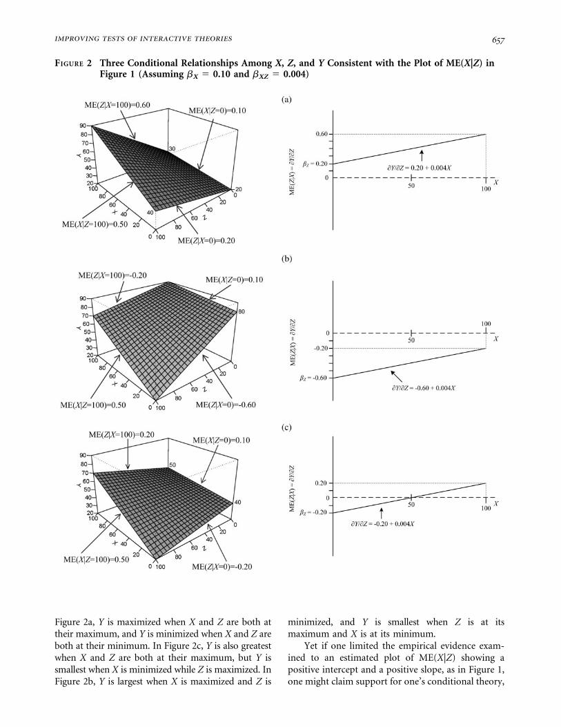
Figure 2a, Y is maximized when X and Z are both attheir maximum, and Y is minimized when X and Z areboth at their minimum. In Figure 2c, Y is also greatestwhen X and Z are both at their maximum, but Y issmallest when X is minimized while Z is maximized. InFigure 2b, Y is largest when X is maximized and Z is

minimized, and Y is smallest when Z is at itsmaximum and X is at its minimum.

Yet if one limited the empirical evidence exam-ined to an estimated plot of ME(X|Z) showing apositive intercept and a positive slope, as in Figure 1,one might claim support for one’s conditional theory,

FIGURE 2 Three Conditional Relationships Among X, Z, and Y Consistent with the Plot of ME(X|Z) inFigure 1 (Assuming bX 5 0.10 and bXZ 5 0.004)


ignorant of the inconsistent evidence that would beapparent from an inspection of a plot of ME(Z|X).Thus, even when there is strong empirical support fora hypothesis about how the marginal effect of X on Yvaries with Z based on an estimated plot of ME(X|Z), afailure to use one’s conditional theory to derive anadditional hypothesis about how the marginal effect ofZ varies with X (beyond a prediction about the valueof bXZ) and inspect a marginal effect plot for Z maymask either (1) additional evidence in support of thetheory, or more worryingly, (2) evidence inconsistentwith the theory.

It is important to recognize that once one con-structs a theory positing interaction between X and Zin influencing Y specific enough to establish the signsof the intercept and slope of a plot for ME(X|Z), oneneed not demand a great deal more of the theory togenerate additional predictions about ME(Z|X)that would permit a stronger test of the theory. Forexample, assume once more that one’s theory pre-dicts a plot of ME(X|Z) taking the form of Figure 1,with both a positive intercept and a positive slope.We have seen that, by itself, this prediction is con-sistent with all three plots of ME(Z|X) in Figure 2. But ifthe theory were to predict additionally that Z has apositive effect on Y when X is at, say, its highest (or, infact, any) value, then this would imply that Figure2b—for which ME(Z|X) is negative throughout—isinconsistent with the theory. If, in contrast, the theorywere to predict that Z has a positive effect on Y when Xis at its lowest value, then both Figures 2b and 2c wouldbe eliminated as possibilities. In both of these cases,supplementing an estimated plot of ME(X|Z) with oneof ME(Z|X) would allow for a stronger test of theunderlying conditional theory.

Deriving and Testing as ManyPredictions as a Conditional

Theory Allows

We now offer some practical advice on deriving andtesting hypotheses from conditional theories that canbe accurately specified with the linear-interactivemodel of equation (1).

Five Key Predictions

Ideally, a theory positing interaction between X and Zin influencing Y would be strong enough to predictthe precise magnitude of the effect of each of X and Zat every possible value of the other variable. Of

course, theories in political science are very rarelystrong enough to generate such specific predictions.However, we believe that conditional theories in theliterature are typically strong enough to generate fivebasic predictions about the marginal effects of X andZ on Y:8

1. PX jZmin: The marginal effect of X is [positive,

negative, zero] when Z is at its lowest value.2. PX jZmax

: The marginal effect of X is [positive,negative, zero] when Z is at its highest value.

3. PZjXmin: The marginal effect of Z is [positive,

negative, zero] when X is at its lowest value.4. PZjXmax

: The marginal effect of Z is [positive,negative, zero] when X is at its highest value.9

5. PXZ: The marginal effect of each of X and Z is[positively, negatively] related to the othervariable.

Note that by calling for researchers to state predic-tions about what happens when X and Z are at theirlowest and highest values, we do not imply thatanalysts should necessarily focus greatest attention onestimated marginal effects at these extreme values.Indeed, as we note below, when there are fewobservations at these extremes, estimates of marginaleffects at these values are less relevant for testing thetheory than estimates of marginal effects at morecentral values for X and Z. Rather, we call for pre-dictions at the extremes simply because if one assumeslinearity as in equation (1), or at least monotonicity,such predictions automatically imply predictions atvalues between the extremes.10

The predictions outlined above need not be pre-sented as five separate hypotheses. Indeed, with careful

8These predictions are based on the case in which an author’sconditional theory conforms to a model of the form shown inequation (1). More complex conditional theories would producetestable predictions of a different form and require an alternativemodel specification.

9Two issues regarding these predictions are worth noting. First,when Z is dichotomous, the predictions PZjXmin

and PZjXmaxshould

be stated in terms of the response of Y to a discrete change in Zrather than in terms of the marginal effect of Z. This is because theconcept of a marginal effect makes sense only when it is possible toconceive of an infinitesimally small change in Z. The predictionsPX jZmin

and PX jZmaxshould be stated similarly when X is dichoto-

mous. Second, when any of these predictions points to a zeroeffect, in which one independent variable has no effect at anextreme value of the other, scholars need to think very carefullyabout whether the functional form of equation (1) properlyspecifies the expected nature of the interaction (see the appendix).

10Of course, when one independent variable—say X—is dichoto-mous, the highest and lowest values of X are the only two possiblevalues for X, and thus the predictions PZjXmin

and PZjXmaxtogether

describe the marginal effect of Z at all possible values of X.


phrasing, all five predictions can be subsumed in asingle hypothesis about how the marginal effect of Xvaries with Z and a single hypothesis about how themarginal effect of Z varies with X. This is illustratedin the following pair of hypotheses:

d HX|Z: The marginal effect of X on Y is positive at allvalues of Z; this effect is strongest when Z is at itslowest and declines in magnitude as Z increases.

d HZ|X: The marginal effect of Z on Y is positive whenX is at its lowest level. This effect declines inmagnitude as X increases; at some value of X, Zhas no effect on Y. As X rises further, the effect of Zbecomes negative and strengthens in magnitude asX increases.

Note that HX|Z implies that the marginal effect of X ispositive at both the lowest and highest values of Z,thereby offering predictions PX jZmin

and PX jZmax. HZ|X

states that the marginal effect of Z is positive at X’slowest value and negative at X’s highest value, therebyoffering predictions PZjXmin

and PZjXmax. There is no

need to state a separate hypothesis that each inde-pendent variable is negatively related with the marginaleffect of the other because such a prediction—that ofPXZ—is implicit in both HX|Z and HZ|X. Thus, incombination, HX|Z and HZ|X include all five predic-tions we recommend and offer as complete a descrip-tion of the expected interaction between X and Z asone could offer for a linear-interactive model withoutpredicting specific magnitudes for marginal effects atspecific values of the independent variables.

In general, scholars who propose a theory shouldseek to test as many of the theory’s implications aspossible. When it comes to interactive theories thatcan be accurately specified by the linear model ofequation (1), this requires making, and then testing,as many of the five predictions listed above aspossible. Later, we illustrate this recommendationby revisiting two recent studies estimating an inter-active model—one in comparative politics and one ininternational relations—and considering whethereach utilizes the model’s coefficient estimates to testall of the predictions that the author’s theory gen-erates. Before we do this, though, we briefly discussseveral issues that arise when evaluating empiricalevidence in favor of, or against, conditional theories.

Some Prototypical Results When TestingInteractive Models

Suppose we want to evaluate the empirical supportfor the conditional theory from which hypothesesHX|Z and HZ|X in the previous section are derived

following the advice we have offered. We would esti-mate equation (1) and then use the model’s coefficientsto construct marginal effect plots for both X and Z.Clearly, the evidence in favor of the theory would begreatest in the case where we find strong support foreach of the five predictions made by hypotheses HX|Z

and HZ|X. This would involve finding that the pointestimates for ME(X|Z 5 zmin), ME(X|Z 5 zmax), andME(Z|X 5 xmin) are all positive, statistically signifi-cant, and substantively significant; and that the pointestimates for ME(Z|X 5 xmax) and bXZ are bothnegative, statistically significant, and substantivelysignificant [where ‘‘min’’ and ‘‘max’’ refer to theminimum and maximum observed values of a variablein the sample]. Below, when we use the term ‘‘sig-nificant’’ without any qualification, it is meant toimply that both statistical and substantive significancehave been established.11

But should we require that all of these conditionsbe met before we claim any empirical support for ourconditional theory and reject our theory if any of theconditions is not achieved? Ultimately, we believethat this is an unrealistically strong standard forempirical evidence and that it would be a mistaketo treat all situations in which at least one of theseconditions fails to be met as equivalent. Althoughfirm knowledge that one of the five predictions fromearlier is false would be sufficient logical grounds forconcluding that the underlying theory is false, it isimportant to remember that statistical tests cannottell us with certainty whether any of the predictions isfalse; all they offer is information about the risks of afalse inference if one rejects the null hypothesis that aquantity of interest equals a particular value, usuallyzero. For this reason, it is inappropriate to establish‘‘hard and fast’’ rules about what combinations ofevidence regarding the five predictions constitutesupport for the underlying conditional theory.

Nevertheless, we can examine several prototypicalsets of results one might get when estimating aninteractive model taking the form of equation (1),

11Unless we explicitly state to the contrary, ‘‘statistically signifi-cant’’ in this article implies significantly different from zero atsome specified significance (a) level. When we say that a pointestimate is ‘‘substantively significant,’’ we mean that its valueis large enough to be deemed of nontrivial magnitude. Werecognize that the minimum magnitude required for substantivesignificance is subjective and that there is no single correct way ofestablishing substantive significance. In our replication of a studyby Alexseev (2006) later in the article, we illustrate one potentiallyuseful strategy for demonstrating the substantive significance ofinteractive relationships. For more on the important differencebetween statistical and substantive significance, see Achen (1982,41–51).


and for each, assess the extent to which we would feelcomfortable claiming support for the underlyingconditional theory given the empirical evidencepresented. To ground the discussion, assume we seekto test the theory generating hypotheses HX|Z andHZ|X. A strong test would require that we use themodel’s coefficient estimates to evaluate all five ofthe predictions contained in HX|Z and HZ|X. How-ever, for illustrative purposes, we simplify mattersin the discussion that follows by focusing on hypoth-esis HX|Z and the three predictions that it contains:(1) ME(X|Z 5 zmin) . 0, (2) ME(X|Z 5 zmax) . 0,and (3) bXZ , 0.

Six different prototypical sets of results areportrayed in Figure 3 in the form of a marginal effectplot for X. The dashed curves around the marginaleffect line depict a 95% confidence interval, therebyidentifying the values of Z at which the marginaleffect of X is statistically significant. However, sincewe want the plots to convey information aboutsubstantive significance as well, we identify the valuesof Z at which the marginal effect of X on Y issignificant (i.e., both statistically and substantivelysignificant) by making the horizontal axis bold atthese values.12 Under each plot, we also indicatewhether the coefficient on the product term, bXZ, issignificant. This last piece of information is notusually included in published marginal effect plotsbut is critical for determining whether there isempirical evidence of interaction between X and Z,i.e., for testing prediction PXZ.13 This is because, asequation (4) reminds us, bXZ indicates the strength of

the relationship between both (1) ME(X|Z) and Z,and (2) ME(Z|X) and X:

@Y

@X@Z¼ @Y

@Z@X¼ bXZ : ð4Þ

To facilitate readers seeing as much statistical evidencerelevant for testing a theory positing interaction aspossible, we recommend that scholars routinely reportthe estimated product-term coefficient and a t-ratio orstandard error for this coefficient in their marginaleffect plots.

Consider first the plot in Figure 3a. The marginaleffect of X is positive and significant across the ob-served range of Z, and bXZ is negative and significant.This plot provides unambiguously strong evidence forhypothesis HX|Z because each of its three predictionsreceives strong empirical support. Next, consider theplot shown in Figure 3b. The only difference here is thatthe marginal effect of X is no longer significant when Zis at its highest value. However, because HX|Z predictsthat the marginal effect of X on Y declines in magnitudeas Z increases, which leaves open the possibility of aweak effect by the time Z gets large, we are notparticularly troubled to find that ME(X|Z 5 zmax) failsto be significant. Thus, in this situation, we wouldconclude that there is strong support for HX|Z eventhough the value for ME(X|Z 5 zmax) is notsignificant.14

The plot shown in Figure 3c provides a moreambiguous case. As before, the significant coefficienton the product term represents clear evidence thatthe marginal effect of X is conditional on Z aspredicted. The difference is that the range of valuesfor Z for which the marginal effect of X is positiveand significant is now smaller than in Figure 3b, andthe point estimate for ME(X|Z 5 zmax) is actuallynegative. In this scenario, we are not terribly con-cerned that the point estimate for ME(X|Z 5 zmax)takes the ‘‘wrong’’ sign because this value is statisti-cally and substantively insignificant. We would arguethat how supportive these results are of hypothesisHX|Z depends on the percentage of observationshaving values of Z at which the marginal effect of Xis positive and significant, i.e., for which Z , z’’ inthe figure. The higher this percentage, the more

12We adopt this ‘‘bold’’ axis convention here because it is usefulfor portraying and discussing hypothetical results about ‘‘generic’’X, Y, and Z variables. We do not recommend that researchersadopt this convention when reporting actual research results.

13Note that whether this is true for models with limited dependentvariables like logit and probit depends on the dependent variableof conceptual interest. There are two possible dependent variablesof conceptual interest when estimating a binary logit or probitmodel: (1) an unbounded latent variable, Y*, assumed to bemeasured by the observed dichotomous variable, Y, and (2) theprobability that Y equals one, Pr(Y 5 1). When one’s dependentvariable of interest is the unbounded Y*, then the product-termcoefficient, bX Z, reflects the extent of interaction. However, this isnot the case when the dependent variable of interest is Pr(Y 5 1).Indeed, when the dependent variable is Pr(Y 5 1), one cannotdetermine whether there is interaction between X and Z byinspecting the coefficient on the product term (or any singleterm). The fact that the marginal effect of each of X and Z onPr(Y 5 1) is not linearly related to the other variable means thatprediction PXZ must be evaluated by estimating the marginaleffects of X and Z at different values for the independent variablesand assessing how they change as the values of the independentvariables change (Ai and Norton 2003; Berry, DeMeritt, and Esarey2010; Norton, Wang, and Ai 2004).

14Ideally, the theory underlying HX|Z would be strong enough togenerate a prediction about whether the marginal effect of X on Yshould (1) remain strong even when Z reaches its maximum, or(2) decline to near zero when Z is maximized. In the former case,the theory would predict that X has a significant effect on Y whenZ 5 zmax. But in the latter case, it would predict an insignificanteffect when Z 5 zmax. Admittedly, theories in political science arerarely capable of yielding such a fine distinction.


inclined we would be to accept the empirical evidenceas supportive. Of course, the minimum percentagehigh enough to justify a claim of support is subjective.As a result, we recommend that scholars report thepercentage of observations that fall within the regionof significance. Indeed, it would be very helpful ifresearchers would provide a frequency distribution forthe variable plotted on the horizontal axis so thatreaders can assess for themselves the relative density ofobservations across the range of X. We illustrate howsuch a frequency distribution might be incorporated

into a marginal effect plot when we report the resultsof two replications in the next section.

When it comes to evaluating conditional theories,one practice that we strongly advise against is gettinginto a ‘‘counting game’’ in which one’s conclusion isbased strictly on the number of predictions for whichthere is statistical support. For example, consider theplot shown in Figure 3d. This plot provides statisticalconfirmation for two of the three predictions con-tained in HX|Z, namely that ME(X|Z 5 zmin) ispositive and that bXZ is negative. The fact that bXZ

FIGURE 3 Plots of ME(X|Z) Reflecting Several Prototypical Sets of Empirical Results


is significant provides strong empirical evidence ofinteraction between X and Z. Importantly, though,the plot suggests that this interaction takes an appre-ciably different form than that predicted by hypothesisHX|Z. Although X has the expected positive effect whenZ is low, X has a significant negative effect when Z getslarge. We believe that scholars should not sweep thiskind of inconsistency with the hypothesis ‘‘under therug’’ by claiming a healthy ‘‘batting average’’ of 0.667,with two of the three predictions confirmed. Evidencethat when Z is high, increases in X yield substantialdecreases in Y rather than the predicted increases strikesus as sufficient to raise serious concerns about theconditional theory underlying the hypothesis.

Figure 3e illustrates a more extreme case in whichclaiming support for HX|Z based on two of the threepredictions receiving statistical support would beunwarranted. In this case, the marginal effect of Xis positive and significant across the entire observedrange of Z, thereby indicating support for the predict-ions that ME(X|Z 5 zmin) and ME(X|Z 5 zmax) arepositive. However, although bXZ is negative aspredicted, it lacks statistical significance and the nearlyflat marginal effect line indicates that the magnitude ofbXZ is substantively trivial. In essence, there is noevidence of appreciable interaction between X and Z.Indeed, this sort of plot—with a marginal effect linesloped slightly upward or downward—is exactly whatwe would expect to find if we were to estimate equation(1) when each of X and Z has a strong positive effect onY but their effects are additive rather than interactive.Thus, the evidence in Figure 3e seriously challenges thetheory predicting that X and Z interact in influencing Y.

We now consider a final set of prototypicalresults shown in Figure 3f. Once again, the lineplotted is intended to be nearly flat. The effect of Xon Y is substantively insignificant at all values of Z,but statistically significant when Z , z’’’. The factthat the marginal effect of X changes from statisticallysignificant when Z , z’’’ to statistically insignificantwhen Z $ z’’’ might seem to suggest that there isinteraction between X and Z. Indeed, BCG (2006, 74)imply precisely this when they claim that a situationin which the marginal effect of X on Y is statisticallysignificant for some values of Z but not for othersmight be interpreted as a sign of meaningful inter-action even when the coefficient on the product termis statistically insignificant. However, this is incorrect.The nearly flat line in Figure 3f represents a case inwhich the marginal effect of X has a t-ratio barelyabove the threshold for statistical significance whenZ is low and a t-ratio barely below the threshold whenZ is high. If one capitalizes on the fact that ME(X|Z)

changes from statistically significant to not as Zsurpasses z’’’ to claim evidence of interaction, oneis placing too much reliance on an arbitrarily chosenlevel of statistical significance. If this level were setslightly higher, ME(X|Z) would be statistically sig-nificant over the entire range for Z. If the level wereset slightly lower, the marginal effect would not bestatistically significant at any value of Z. The morerelevant information is that the coefficient on theproduct term, bXZ, is not statistically significant andis of small magnitude. As we showed in equation (4),this indicates that the marginal effect of X varies onlytrivially with Z, and on this basis we should reject thetheory positing interaction underlying HX|Z.

Two Replications

We now illustrate our central points by replicating twostudies chosen from the many that test a conditionaltheory but that present a marginal effect plot for justone of the two variables hypothesized to interact. Inone replication, examining the second marginal effectplot lends additional support for the researcher’stheory. In the other, the second plot provides evidencethat contradicts the author’s theory.

Revealing Additional Evidence in Favor ofthe Theory Being Tested

Kastner (2007) examines how conflicting interestsand the strength of domestic actors with interna-tionalist economic interests affect the level of tradebetween countries. Previous studies indicate thatbilateral trade tends to be lower when countries haveconflicting political interests. As Kastner notes,though, there is considerable variation across countrydyads in the extent to which conflicting interests leadto reduced bilateral trade. His explanation for thisvariation centers on the strength of domestic actorswho benefit from trade. Specifically, Kastner arguesthat although leaders generally want to reduce tradewith countries that do not share their interests, someleaders are constrained in their ability to do this bythe presence of strong domestic actors with interna-tionalist economic interests. As Kastner puts it, ‘‘thenegative effects of conflict on commerce should beless severe when internationalist economic interestshave strong political clout domestically’’ (2007, 670).Unable to measure the strength of internationalistinterests in a dyad directly, Kastner uses the extent oftrade barriers in the countries (Trade Barriers) as aproxy variable that is inversely related to the strength


of these interests. If we denote the extent of conflictbetween two countries by Conflict and their level ofbilateral trade by Trade, Kastner’s hypothesis can bestated as follows:

d HConflict|Barriers: The marginal effect of Conflict onTrade is negative at all values of Trade Barriers; thisnegative effect is weakest when Trade Barriers is atits lowest level and strengthens in magnitude asTrade Barriers increases.

Kastner tests his conditional theory using annualdata from 76 countries from 1960 to 1992 and anOLS model with an interactive specification takingthe form of equation (1):

Trade ¼ b0 þ bCConflict þ bBTrade Barriers

þ bCB Conflict 3 Trade Barriersð Þþ bControlsþ e;

ð5Þ

where Controls is a vector of control variables. Thecoefficient on the product term, Conflict 3 TradeBarriers, is negative and statistically significant at the0.01 level, with a t-statistic of -5.26. Using the param-eter estimates from his model (Table 1, Model 1, 676),Kastner produces a plot showing how the marginaleffect of Conflict on Trade varies with the level ofTrade Barriers. We reproduce this marginal effect plotin a slightly modified form in Figure 4a.15 Based on theplot, as well as the statistically significant negative coef-ficient on the product term, Kastner claims empiricalsupport for his theory.

We advise researchers who propose a theorypositing interaction between two variables, X and Z,to use the theory to generate as many of the five keypredictions listed earlier as the theory allows regard-ing the marginal effects of X and Z on Y. Kastner’s

hypothesis, HConflict|Barriers, offers three of thesepredictions:

d PCjBmin: The marginal effect of Conflict on Trade is

negative when Trade Barriers is at its lowest value.d PCjBmax

: The marginal effect of Conflict on Trade isnegative when Trade Barriers is at its highest value.

d PCB: The marginal effect of each of Conflict andTrade Barriers is negatively related to the othervariable.

However, Kastner’s hypothesis is silent about theexpected value (positive, negative, or zero) of themarginal effect of Trade Barriers at the highest andlowest values of Conflict.

Before we consider the marginal effect of TradeBarriers on Trade, we reevaluate the empirical supportfor predictions PCjBmin

, PCjBmax, and PCB. Assuming that

the statistically significant negative coefficient for theproduct term in equation (5) is also substantivelysignificant, there is unambiguous support for predic-tion PCB.16 In other words, there is clear evidence thatthe marginal effect of Conflict on Trade is negativelyrelated to the value of Trade Barriers, as Kastnerhypothesizes, and (due to the symmetry of interac-tions) that the marginal effect of Trade Barriers isnegatively related to the value of Conflict.

But is this conditionality consistent with predic-tions PCjBmin

and PCjBmax? On the one hand, Figure 4a

shows that the marginal effect of Conflict is negativeand statistically significant when Trade Barriers takeson its largest observed value, thereby supportingprediction PCjBmax

. On the other hand, predictionPCjBmin

fails to receive empirical support. Contrary toexpectation, the marginal effect of Conflict is positiveand statistically significant when Trade Barriers is atits smallest observed value, and indeed, at all valuesless than 3.16. Overall, the marginal effect plot forConflict closely resembles the prototypical plot shownin Figure 3d. This raises concerns about the condi-tional theory underlying the hypothesis being testedbecause the estimated marginal effect is statisticallysignificant in the ‘‘wrong’’ direction at one end of thehorizontal axis. Kastner offers no explanation forwhy an increase in conflict should lead to increasedbilateral trade when domestic actors with internation-alist economic interests are strong, i.e., when trade

15We were able to replicate Kastner’s results perfectly. Ourmarginal effect plot differs from his (Figure 1, 677) in fourrespects. Rather than plotting the marginal effect of Conflict onTrade on the vertical axis, as we do, Kastner plots the change inTrade as Conflict increases from its 15th percentile in the sampleto its 85th percentile. Given the linear form of equation (5), thisdifference in scaling the vertical axis is superficial because onescaling is a linear transformation of the other. Second, Kastnerplots percentiles for Trade Barriers in the sample along thehorizontal axis. We saw no good reason to distort the scale forTrade Barriers by using percentiles rather than the actual values.This difference in scaling for the horizontal axis explains why ourplot is linear, but Kastner’s is not. Third, we plot the marginaleffect of Conflict on Trade over the entire range of values forTrade Barriers in the estimation sample, whereas Kastner plots itonly over the values for Trade Barriers that fall between the 20th

and 80th percentiles. Fourth, we have added a shaded rectangle toour plot; we explain the purpose of this below.

16Kastner does not explicitly evaluate the substantive significanceof the estimated effects he reports. Rather than undertake ourown assessment, for our illustration we simply assume that‘‘statistical significance’’ implies ‘‘significance’’ (i.e., both statis-tical and substantive significance).


barriers are low. In our view, the statistically sig-nificant positive effect of Conflict when TradeBarriers is less than 3.16 should not be dismissedas a trivial inconsistency; rather, it is an importantpiece of evidence to consider alongside the supportfor predictions PCjBmax

and PCB when evaluatingKastner’s theory.

Our replication of Kastner’s analysis illustratesthe importance of constructing a marginal effect plotthat shows how the effect of X on Y varies over theentire observed range of Z. Kastner plots the marginaleffect of Conflict only for values of Trade Barriersbetween the 20th and 80th percentiles; this interval isindicated by the shaded rectangle in Figure 4a. Notethat in this restricted range for Trade Barriers, theestimated marginal effect of Conflict on Trade,although positive for low values of Trade Barriers, isnever positive and statistically significant. Thus,although the full marginal effect plot reveals valuesfor Trade Barriers at which there is clear evidence ofan unexpected positive effect of Conflict on Trade, therestricted plot masks the existence of these values andmakes it appear as if the estimated positive effect ofConflict never achieves statistical significance even atthe lowest values for Trade Barriers. Indeed, Kastner’srestricted plot more closely parallels the prototypicalplot shown in Figure 3c, which we argued earlierpotentially offers support for the hypothesis beingtested depending on the percentage of sample ob-servations falling into the region of significance.

Consider the results in Figure 4a more closely.The marginal effect of Conflict is negative andstatistically significant when Trade Barriers exceeds3.41. Superimposed over the marginal effect plot is ahistogram portraying the frequency distribution forTrade Barriers; the scale for the distribution is givenby the vertical axis on the right-hand side of thegraph. The histogram shows that 55.4% of thecountry dyads in Kastner’s sample fall into this rangeof statistical significance. At the other extreme, theeffect of Conflict is positive and statistically significantwhen Trade Barriers is less than 3.16. Of the sampleobservations, 14.5% lie in this range.17 Althoughthese latter observations, which are inconsistent with

FIGURE 4 Marginal Effect Plots Designed toEvaluate the Conditional TheoryPresented by Kastner (2007)

17The fact that there are few observations at low levels of TradeBarriers means that the evidence that Conflict has a statisticallysignificant positive effect on Trade when Trade Barriers is lowmay rest heavily on the model’s linearity assumption. (Note thatreaders would be completely unaware of this issue in the absenceof a histogram showing the dearth of sample observations withlow values of Trade Barriers. This highlights the importance ofincluding in a marginal effect plot information about thedistribution of the variable depicted on the horizontal axis.)Unless one believes that there is a strong a priori theoreticaljustification for the linearity assumption, one should be skepticalabout drawing strong inferences concerning the marginal effectof Conflict at low levels of Trade Barriers without subjecting thisassumption to empirical scrutiny. In the online appendix athttp://journals.cambridge.org/jop, we do precisely this by esti-mating quadratic and cubic versions of Kastner’s model, therebyrelaxing the linearity assumption. The evidence that Conflict has astatistically significant positive effect on Trade when TradeBarriers is low is robust to these alternative specifications.


Kastner’s theory, do not constitute a large percentageof the sample, they are far from being a trivial set ofoutlier observations.

Of course, the primary point of this article is thatit may be a mistake to draw any conclusion aboutKastner’s theory based solely on the coefficientestimate for the product term and the marginal effectplot shown in Figure 4a. We should also determinewhether Kastner’s conditional theory generates pre-dictions about the marginal effect of Trade Barrierson Trade across the range of values for Conflict and, ifso, determine whether these predictions receiveempirical support. Although Kastner provides noexplicit hypothesis about the effect of internationalisteconomic interests on bilateral trade, his underlyingtheory is not silent on the matter. As Kastner notes,‘‘leaders who depend on support from actors whobenefit from trade pay, at the margins, higherdomestic political costs for placing restrictions onforeign commerce than do other leaders’’ (2007, 670).This line of reasoning leads to the prediction thatstronger internationalist economic interests amongdomestic groups will prompt increased bilateral tradeirrespective of the level of conflict between countries.Given that the proxy variable, Trade Barriers, isinversely related to the strength of internationalisteconomic interests, Kastner’s theory implies thefollowing new hypothesis:

d HBarriers|Conflict: The marginal effect of Trade Bar-riers on Trade is negative at all values of Conflict.This negative effect is weakest when Conflict is at itslowest level and increases in magnitude as Conflictincreases.18

This hypothesis yields two predictions that togetherwith PCjBmin

, PCjBmax, and PCB constitute the full set of

five predictions that we delineated earlier:

d PBjCmin: The marginal effect of Trade Barriers on

Trade is negative when Conflict is at its lowestvalue.

d PBjCmax: The marginal effect of Trade Barriers on

Trade is negative when Conflict is at its highestvalue.

In Figure 4b, we plot the estimated marginaleffect of Trade Barriers across the observed range ofConflict values. This graph provides strong supportfor the two new predictions, and thus, Kastner’sconditional theory. As expected, Trade Barriers hasa statistically significant negative marginal effect on

Trade across the entire observed range for Conflict.By failing to (1) make explicit some of the predictions(PBjCmin

and PBjCmax) that are clearly implied by his

theory and (2) construct a marginal effect plot that canbe used to evaluate these predictions, Kastner fails torecognize empirical evidence in support of his theory.Readers seeking to assess Kastner’s theory shouldconsider both plots shown in Figure 4, as well as theestimated product-term coefficient. They shouldweigh the considerable evidence consistent with theunderlying theory against the contradictory findingthat the marginal effect of Conflict is significantlypositive over a range of values for Trade Barriersaccounting for 14.5% of Kastner’s sample observa-tions. Regardless of the importance one attaches tothe evidence that is in conflict with Kastner’s theory,it is certainly the case that the information derived byconstructing a second marginal effect plot adds to theevidence in support of his theory.

Revealing Additional Evidence Contrary tothe Theory Being Tested

Alexseev (2006) examines how changes in the ethniccomposition of Russia’s regions affect the vote sharewon by the extreme Russian nationalist ZhirinovskyBloc in the 2003 elections to the Russian State Duma.Alexseev investigates the ability of three competingtheories—the ‘‘power threat’’ model, the ‘‘powerdifferential’’ model, and the ‘‘defended nationhood’’model—to explain the level of electoral supportreceived by the Zhirinovsky Bloc. Ultimately, Alexseevconcludes that the defended-nationhood model pro-vides the best explanation. According to this model,support for anti-immigrant parties (Xenophobic Voting)depends on the percentage of the population in aregion belonging to the dominant ethnic group andthe change in the percentage of the populationaccounted for by ethnic minorities (2006, 218–20).More specifically, an increase in the size of thedominant ethnic group should enhance the supportfor anti-immigrant parties, and this positive effectshould be greater in regions that have experienced alarge influx of ethnic minorities. Moreover, the changein the percentage of the population comprised ofethnic minorities should have a positive effect onsupport for anti-immigrant parties regardless of thesize of the dominant ethnic group. In Russia, Slavsconstitute the dominant ethnic group. Thus, in theRussian context, Alexseev’s defended-nationhood hy-pothesis can be stated as follows:

d HAlexseev: The marginal effect of the size of thedominant ethnic group (Slavic Share) on support

18This sentence is implicit in hypothesis HConflict|Barriers due to theinherent symmetry of interactions.


for the Zhirinovsky Bloc (Xenophobic Voting) isalways positive; this positive effect grows instrength as the increase in the share of thepopulation comprised by ethnic minorities(Dnon-Slavic Share) gets larger (or the decrease inDnon-Slavic Share gets smaller). The marginaleffect of Dnon-Slavic Share on Xenophobic Votingis positive at any value for Slavic Share.

Alexseev tests this hypothesis using data from 72Russian regions and an OLS model with an inter-active specification in the form of equation (1):

Xenophobic Voting ¼ b0 þ bS Slavic Share

þ bN Dnon-Slavic Share

þ bSNðSlavic Share

3 Dnon-Slavic ShareÞþ bControlsþ e;

ð6Þ

where Controls is a vector of control variables. Using theparameter estimates from this model (Table 2, Test 1,225), Alexseev produces a plot showing how themarginal effect of Slavic Share on Xenophobic Votingvaries with Dnon-Slavic Share. We reproduce this plotin Figure 5a.19 Based on this plot, Alexseev claimsempirical support for the defended-nationhood model.

Note that Alexseev’s hypothesis contains the fullset of five predictions we urge scholars with condi-tional theories to offer readers:

d PSjNmin: The marginal effect of Slavic Share on

Xenophobic Voting is positive when Dnon-SlavicShare is at its lowest value.

d PSjNmax: The marginal effect of Slavic Share on

Xenophobic Voting is positive when Dnon-SlavicShare is at its highest value.

d PN jSmin: The marginal effect of Dnon-Slavic Share on

Xenophobic Voting is positive when Slavic Share isat its lowest value.

d PN jSmax: The marginal effect of Dnon-Slavic Share on

Xenophobic Voting is positive when Slavic Share isat its highest value.

d PSN: The marginal effect of each of Slavic Share andDnon-Slavic Share is positively related to the other

variable.

Although Alexseev’s hypothesis yields all five of thepredictions that we recommend, he evaluates only

three of them: PSjNmin, PSjNmax

, and PSN. We begin by

reevaluating the support for these three predictions.

FIGURE 5 Marginal Effect Plots Designed toEvaluate the ‘‘Defended Nationhood’’Model Presented by Alexseev (2006)

19We were unable to replicate Alexseev’s OLS results perfectly.However, our results are extremely close to his. Indeed, the ratio ofthe coefficient with the larger magnitude across the two estima-tions to the coefficient with the smaller magnitude was less than1.01 for all but one regressor; for the one exception, the ratio was1.016. Not surprisingly, the lines on our respective marginal effectplots are visually indistinguishable. The only other differencebetween our marginal effect plot and Alexseev’s is that we showthe marginal effect of Slavic Share across the full range of values forDnon-Slavic Share in the sample (including negative values thatindicate that the non-Slavic population share is decreasing),whereas Alexseev truncates the horizontal axis at zero.


In line with prediction PSN, the coefficient on theproduct term is positive, indicating that the marginaleffect of each of Slavic Share and Dnon-Slavic Share ispositively related to the other variable. Although thecoefficient on the product term is not statisticallysignificant at the 0.05 level in the two-tail test thatAlexseev reports, it is significant at the 0.10 level in atwo-tail test or, equivalently, at the 0.05 level in a one-tail test. Given the relatively small sample size (n 5 72)and the fact that the coefficient is very close to beingstatistically significant at standard levels, we wouldnot be prepared to reject Alexseev’s theory on thisground alone.

For further relevant information, it is useful toassess the magnitude of the interaction reflected bythe point estimate for the product term in moresubstantive terms. Our goal is to determine whetherthe estimated marginal effect of Slavic Share onXenophobic Voting changes by a nontrivial amountas Dnon-Slavic Share changes. We first note that thereis substantial variation in Xenophobic Voting withinAlexseev’s sample. For example, the electoral supportfor the Zhirinovsky Bloc ranges from 2.8% to 19.5%across the Russian regions. The product-term coef-ficient can be used to predict the response ofXenophobic Voting to an increase in Slavic Share fromits lowest value (27.4) in the sample to its highestvalue (98.9) at both the lowest (-1.93) and highest(12.99) values of Dnon-Slavic Share. When Dnon-Slavic Share is at its lowest value, a shift across therange for Slavic Share produces an expected increaseof 1.11 in the Zhirinovsky vote percentage. Thisexpected increase amounts to just 6.7% of the rangeof Xenophobic Voting in the sample and, therefore,indicates a substantively trivial estimated effect. Instark contrast, a shift across the range for Slavic Sharewhen Dnon-Slavic Share is at its highest valueprompts an expected increase of 9.89 in the Zhir-inovsky vote percentage, a value equal in magnitudeto 59.2% of the range of Xenophobic Voting in thesample. This indicates that Slavic Share has a strongeffect in the expected direction when Dnon-SlavicShare is at its highest. This large variation in thesubstantive magnitude of the effect of Slavic Shareacross different values of Dnon-Slavic Share, alongwith the near statistical significance of Alexseev’sproduct-term coefficient in a small sample, leads usto conclude that there is empirical support forprediction PSN.

Predictions PSjNminand PSjNmax

together imply thatthe marginal effect of Slavic Share on XenophobicVoting is positive for all values of Dnon-Slavic Share.The plot in Figure 5a shows that the point estimate of

the marginal effect of Slavic Share is, indeed, positiveat all values of Dnon-Slavic Share. However, themarginal effect is statistically significant only whenthe change in the non-Slavic share of the populationexceeds 0.93. This marginal effect plot is similar tothe prototypical plot in Figure 3b. Given that thepositive marginal effect of Slavic Share is predicted todecline in magnitude as Dnon-Slavic Share decreases,a weak effect of Slavic Share at low values ofDnon-Slavic Share is not at odds with hypothesisHAlexseev. Thus, we do not view the lack of statisticalsignificance of Slavic Share’s effect over part of therange of the plot in Figure 5a as an indication thatAlexseev’s defended-nationhood model lacks empiri-cal support.

Once again, however, our principal point is thatresearchers should test as many implications of theirconditional theories as possible. The marginal effectplot in Figure 5a and the product-term coefficientprovide the information necessary to evaluate pre-dictions PSjNmin

, PSjNmax, and PSN, but not predictions

PN jSminand PN jSmax

. We can evaluate the latter twopredictions, though, by producing a marginal effectplot for Dnon-Slavic Share. This graph is shown inFigure 5b. According to predictions PN jSmin

andPN jSmax

, the marginal effect of Dnon-Slavic Shareshould always be positive. Contrary to expectations,however, the point estimate of the marginal effect ofDnon-Slavic Share is uniformly negative. Moreover, itis statistically significant when the Slavic share of thepopulation is less than 77.4%, and in our view, it issubstantively significant throughout this range as well.20

The superimposed frequency distribution for SlavicShare, this time shown in the form of a histogram anda rug plot, illustrates that 22% (or 16) of Russia’s 72regions fall into this region of significance. The bottomline is that although the defended-nationhood modelpredicts that larger increases in the concentration ofethnic minorities in a population will lead to moreextensive xenophobic voting, Alexseev’s results actuallyindicate that larger increases will reduce support foranti-immigrant parties, and significantly so over anontrivial range of values for Slavic Share.

20Even at the right edge of this range when Slavic Share is 77.4%,an increase in Dnon-Slavic Share from its lowest to its highestobserved value reduces the expected Zhirinovsky vote percentageby 3.2, a value equal to 19.2% of the range of Xenophobic Voting.When Slavic Share is at its minimum (27.4%), the same change inDnon-Slavic Share decreases the Zhirinovsky vote percentage by9.34—equivalent to 55.9% of the range of Xenophobic Voting.


What is the relevance of the new evidencepresented in Figure 5b? In our view, the addition ofthis new information means that although there isevidence that Slavic Share and Dnon-Slavic Shareinteract to influence Xenophobic Voting, the form ofthis conditionality is sufficiently different from thatpredicted to cast substantial doubt on Alexseev’sdefended-nationhood model. To square the resultsin Figure 5b with the defended-nationhood model,one would have to reframe the theory to be consistentwith the fact that larger increases in the concentrationof ethnic minorities result in less xenophobic voting.Some may consider the inconsistent evidence inFigure 5b to be less important than we do. Ulti-mately, each reader can come to her own conclusionabout this. Nevertheless, it seems indisputable thatthe level of support afforded Alexseev’s theory by thefull set of empirical results—including both marginaleffect plots—is lower than the apparent level ofsupport based solely on the partial set of results inthe published paper. Each researcher testing a theoryshould present readers with as much as possible ofthe relevant empirical evidence derivable from themodel’s coefficient estimates so that readers can makea maximally informed evaluation about the validityof the theory. In Alexseev’s case, this means present-ing readers with both of the plots shown in Figure 5.

Maximizing the InformationPortrayed in a Marginal

Effect Plot

In the replications presented in the previous section, weillustrate several practices regarding the construction ofmarginal effect plots that we hope will become standardin the political science literature. Most importantly, re-searchers should make the horizontal axis of a marginal-effect plot extend from the minimum observed value inthe sample for the variable being plotted to the maximumobserved value. Plotting marginal effects over a widerrange than this risks misleading readers by portrayingout-of-sample inferences, whereas plotting marginaleffects over a narrower range ignores information thatcan be relevant for evaluating hypotheses.

But not all values for the variable depicted on thehorizontal axis are equally important. For example, ifboth the minimum and maximum values are outliers inthe sample, estimated marginal effects at the extremesare less relevant for assessing the hypothesis underconsideration than marginal effects near the center of

the distribution, where the observations are moreconcentrated.21 Thus, we encourage analysts to super-impose over each marginal effect plot a frequencydistribution for the variable on the horizontal axis togive readers information about the relative density ofdata at different locations. Although it depends tosome extent on the context, we believe that a combi-nation of a histogram and a rug plot has manyvirtues.22 While a histogram provides readers with ageneral overview of the frequency distribution and aquick sense of the percentage of observations that fallinto various regions, a rug plot can be useful because itprovides details about the values of individualobservations.

Finally, we encourage authors to report the esti-mated product-term coefficient along with its t-ratioor standard error somewhere in each marginal effectplot because this is critical information for evaluatinghypotheses about interaction that is not evident fromthe plot itself.

Conclusion

Since the publication of Brambor, Clark, and Golder’s(2006) article, it has become common for politicalscientists to present a marginal effect plot wheninterpreting statistical results for a model positinginteraction between two variables. Scholars im-plementing BCG’s advice have nearly uniformly(1) conceived of one of the variables, say Z, as theconditioning variable, (2) developed a hypothesispredicting how the marginal effect of the othervariable, X, varies with the value of Z, (3) estimateda model specifying interaction between X and Z byincluding a product term, XZ, and (4) constructed amarginal effect plot for X—i.e., a plot of the relation-ship between Z and the estimated marginal effect of Xdesigned to test the hypothesis. Only rarely have

21Even at locations on the horizontal axis closer to the center of thedistribution, there may be ranges of values at which there are fewobservations. It is important to remember that the validity of anyinferences about the marginal effect of a variable at such valuesrests on the linearity assumption of the model being correct. It isnoteworthy that the confidence interval for the marginal effectshown in Figure 5b is actually narrowest at a location on thehorizontal axis at which the data are quite scarce; the width of theconfidence interval at this point is being driven primarily bythe model’s linearity assumption, not the sample observations.

22Much of the value of a rug plot can be lost when the sample sizeis large since individual tick marks blend together and becomeindistinguishable. This explains why we include a rug plot inFigure 5 for the Alexseev replication (n 5 72), but not in Figure 4for the Kastner replication (n . 60,000).


researchers supplemented this hypothesis with a prop-osition about how the marginal effect of Z varies withthe value of X and a corresponding marginal effectplot for Z.

Because of the inherent symmetry of interactions, ahypothesis about the sign (positive or negative) of therelationship between Z and the marginal effect of Xautomatically predicts that the relationship between Xand the marginal effect of Z has the same sign. Whenone’s theory is insufficient to yield additional predic-tions about the relationship between X and themarginal effect of Z, then the restriction of attentionto just one marginal effect plot is appropriate. Buttypically, the conditional theories advanced by politicalscientists do generate additional expectations about therelationship between X and the marginal effect of Z. Insuch situations, a failure to introduce these predictionsand then construct a marginal effect plot for Z suitablefor evaluating them means that researchers are ignor-ing valuable information relevant to testing theirtheory. They are, in effect, subjecting their conditionaltheories to substantially weaker tests than their esti-mation model permits. The consequence is that theliterature exaggerates the empirical support for sometheories and understates the support for others. For-tunately, the fix for the problem is straightforward.Researchers positing interaction between two variablesshould seek to generate hypotheses about how themarginal effect of each variable varies with the value ofthe other and construct a pair of marginal effect plotsto evaluate these hypotheses.

Acknowledgments

We would like to thank Thomas Brambor, WilliamRoberts Clark, Justin Esaray, Robert Franzese, Jeff Gill,Sona Nadenichek Golder, Chris Reenock, David Siegel,Christine Mele, members of the Political InstitutionsWorking Group at Florida State University, and threeanonymous reviewers for helpful comments on earlierversions of this paper. We also thank Scott Kastnerand Mikhail Alexseev for their cooperation and forproviding their replication datasets.

Appendix: When One Variable isExpected to have No Effect at an

Extreme Value of the Other

We have advised scholars who propose an interactivetheory specified in the form of equation (1) to use the

theory to generate as many of the five key predictionslisted in our article as the theory allows. Four of thesepredictions relate to the marginal effect of one in-dependent variable at the lowest or highest value ofthe other. In this appendix, we caution that whenone’s theory posits that one independent variable hasno effect at all (i.e., a marginal effect of zero) whenthe other independent variable is at one of itsextremes, one should think very carefully aboutwhether the functional form of equation (1) isappropriate.

To illustrate why, we will assume that predictionsPX jZmin

and PX jZmaxtake the following form:

d P�1: The marginal effect of X is zero when Z is at itslowest value.

d P�2: The marginal effect of X is positive when Z is atits highest value.

For the theory generating these predictions to beaccurately specified by equation (1)—in which eachindependent variable is assumed to be linearlyrelated to the marginal effect of the other—Z’slowest value must be the only value of Z at whichX has no effect on Y. There are two ways this couldhappen. First, Z could be dichotomous (0 or 1) andX could have no effect on Y when Z 5 0 but apositive effect when Z 5 1. This situation isdepicted in Figure 6a. The second possibility is thatZ is continuous and ME(X|Z) increases linearly withZ when Z . zmin. This situation is depicted inFigure 6b.

But consider the relationship between Z andthe marginal effect of X shown in Figure 6c. Herethe value of Z must surpass some threshold, z’, forX to have any effect on Y, but once this threshold isachieved, ME(X|Z) grows linearly with Z. Condi-tional theories that posit some kind of thresholdeffect similar to that shown in Figure 6c are rela-tively common in political science (Clark, Gilligan,and Golder 2006). For example, Duverger’s theorypredicts that social heterogeneity increases party-system size, but only once the electoral system issufficiently permissive (Clark and Golder 2006).Similarly, Mainwaring (1993) argues that presiden-tialism is bad for democratic survival, but only iflegislative fragmentation is sufficiently high. Theimportant thing to note is that although thethreshold relationship shown in Figure 6c is fullyconsistent with predictions P�1 and P�2, it is notaccurately captured by the linear-interactive spec-ification of equation (1). This is because therelationship between Z and ME(X|Z) is onlypiece-wise linear; it is not linear over the entire


range for Z.23 In this type of situation, an alternativestrategy for model specification and testing is needed.

If one’s theory generates an a priori predictionabout the value of the threshold, z’, then the predictedvalue of z’ can be used to split the sample into twosubsamples. One could then estimate the interactive

model specified in equation (1) separately in thesubsample of observations for which Z # z’ and inthe subsample of observations for which Z $ z’.24 Onewould predict that in the context in which Z is low,ME(X|Z 5 zmin), ME(X|Z 5 z’), and bX Z are all zero.And one would predict that in the context in which Z ishigh, ME(X|Z 5 z’) is zero but both ME(X|Z 5 zmax)and bXZ are positive.

In the more likely situation in which one’s theory isnot strong enough to identify the specific value of thethreshold, z’, the options are less satisfactory. If one isconfident, a priori, that the threshold is much closer tozmin than to zmax, one might reasonably view equation(1) as a sufficiently close approximation of the truemodel to warrant a reliance on this equation forempirical analysis. If one has no expectation aboutthe value of the threshold, one might conduct split-sample estimations of equation (1) multiple times,varying the assumed value of the threshold, and thendetermine the ‘‘correct’’ threshold by comparing the fitsof the various models. Still another option would be toapproximate the expected functional form with aquadratic specification that assumes that the marginaleffect of X changes less abruptly than in Figure 6c,thereby eliminating the need to identify a thresholdvalue for Z altogether. One example of a quadraticspecification that provides a reasonably good fit to thefunctional form shown in Figure 6c is:

Y¼ b0 þ bX X þ bZ Z þ bXZ XZ þ bXZ2 XZ2þ e: ð7Þ

The marginal effect of X in this interactive model is anonlinear function of Z:

MEðXjZÞ ¼ @Y

@X¼ bX þ bXZZ þ bXZ2 Z2: ð8Þ

Note that in equation (7), the marginal effect of Z isnow determined by both X and Z:

MEðZjXÞ ¼ @Y

@Z¼ bZ þ ðbXZ þ 2ZbXZ2ÞX: ð9Þ

FIGURE 6 Marginal Effect Plots Indicating that Xhas No Effect When Z is at itsMinimum Value

23Furthermore, note that if X and Z interact as in Figure 6c, themarginal effect of Z on Y is conditional not only on the value ofX—as in the interactive model in equation (1)—but on the value ofZ as well. It is evident from Figure 6c that when Z # z9, the marginaleffect of X is the same regardless of the value of Z; put differently, Zand X are additive in their effects on Y. The symmetry of interactionimplies that in this range for Z, the marginal effect of Z is unrelatedto the value of X. Figure 6c indicates that when Z $ z9, the marginaleffect of X is positively related to Z. The symmetry of interactionimplies that in this range for Z, the marginal effect of Z is positivelyrelated to X.

24An alternative strategy would be to conduct a full-sampleestimation of a model specifying three-way interaction amongX, Z, and a dichotomous variable, D, that equals 1 when Z . z’and 0 otherwise. In particular, Y would be regressed on X, Z, D,XZ, XD, ZD, and XZD. This estimation would yield pointestimates of marginal effects identical to those obtained usingthe split-sample approach but the standard errors may bedifferent (Kam and Franzese 2007, 103–11).


Put differently, the marginal effect of Z is a linearfunction of X with a different slope at each value of Z.

References

Achen, Christopher. 1982. Interpreting and Using Regression.London: Sage.

Ai, Chunrong, and Edward Norton. 2003. ‘‘Interaction Terms inLogit and Probit Models.’’ Economic Letters 80 (1): 123–29.

Aiken, Leona, and Stephen West. 1991. Multiple Regression: Testingand Interpreting Interactions. London: Sage Publications.

Alexseev, Mikhail A. 2006. ‘‘Ballot-Box Vigilantism: EthnicPopulation Shifts and Xenophobic Voting in Post-SovietRussia.’’ Political Behavior 28 (3): 211–40.

Berry, William D., Jacqueline H. R. DeMeritt, and Justin Esarey.2010. ‘‘Testing for Interaction in Binary Logit and ProbitModels: Is a Product Term Essential?’’ American Journal ofPolitical Science 54 (1): 248–66.

Brambor, Thomas, William Clark, and Matt Golder. 2006.‘‘Understanding Interaction Models: Improving EmpiricalAnalyses.’’ Political Analysis 14 (1): 63–82.

Braumoeller, Bear. 2004. ‘‘Hypothesis Testing and MultiplicativeInteraction Terms.’’ International Organization 58 (4): 807–20.

Clark, William, and Matt Golder. 2006. ‘‘Rehabilitating Duverger’sTheory: Testing the Mechanical and Strategic Modifying Effectsof Electoral Laws.’’ Comparative Political Studies 39 (6): 679–708.

Clark, William R., Michael Gilligan, and Matt Golder. 2006. ‘‘ASimple Multivariate Test for Asymmetric Hypotheses.’’ Polit-ical Analysis 14 (3): 63–82.

Friedrich, Robert. 1982. ‘‘In Defense of Multiplicative Terms inMultiple Regression Equations.’’ American Journal of PoliticalScience 26 (4): 797–833.

Kam, Cindy D., and Robert J. Franzese, Jr. 2007. Modeling andInterpreting Interactive Hypotheses in Regression Analysis. AnnArbor: University of Michigan Press.

Kastner, Scott L. 2007. ‘‘When Do Conflicting Political RelationsAffect International Trade.’’ Journal of Conflict Resolution 51(4): 664–88.

Mainwaring, Scott. 1993. ‘‘The Presidentialism, Multipartism,and Democracy: The Difficult Combination.’’ ComparativePolitical Studies 26 (2): 198–228.

Norton, Edward, Hua Wang, and Chunrong Ai. 2004. ‘‘Comput-ing Interaction Effects and Standard Errors in Logit andProbit Models.’’ Stata Journal 4 (2): 103–16.

Wright, Gerald. 1976. ‘‘Linear Models for Evaluating ConditionalRelationships.’’ American Journal of Political Science 20 (2):349–73.

William D. Berry is Marian D. Irish Professor, andSyde P. Deeb Eminent Scholar at Florida State Uni-versity, Tallahassee, Florida 32303.

Matt Golder is Associate Professor at PennsylvaniaState University, University Park, PA 16802.

Daniel Milton is visiting faculty member atBrigham Young University, Provo, Utah, 84602.


improving test of theories in positing interaction

Documents