Improving Data Quality and Closing Data Gapswith Machine Learning

Tobias Cagala*

May 5, 2017

Abstract

The identification and correction of measurement errors often involves labour intensive case-by-caseevaluations by statisticians. We show how machine learning can increase the efficiency and effective-ness of these evaluations. Our approach proceeds in two steps. In the first step, a supervised learningalgorithm exploits data on decisions to flag data points as erroneous to approximate the results of thehuman decision making process. In the second step, the algorithm applies the first-step knowledgeto predict the probability of measurement errors for newly reported data points. We show that, fordata on securities holdings of German banks, the algorithm yields accurate out-of-sample predictionsand increases the efficiency of data quality management. While the main focus of our analysis is onan application of machine learning to data quality management, we demonstrate that the potential ofmachine learning for official statistics is not limited to the prediction of measurement errors. Anotherimportant problem that machine learning can help to overcome is missing data. Using simulations, weshow that out-of-sample predictions of missing values with machine learning algorithms can help toclose data gaps in a wide range of datasets.

Keywords: Data Quality Management, Measurement Errors, Data Gaps, Machine Learning, SupervisedLearning

*Deutsche Bundesbank, German Securities Holdings Statistics, tobias.cagala@bundesbank.de. The Paper represents theauthor’s personal opinions and does not necessarily reflect the views of the Deutsche Bundesbank or its staff.

1

Further improving and maintaining high data quality is a central goal of official statistics. In the field ofdata quality management (DQM), the collection of data on human decisions in the DQM process createsan opportunity to increase the efficiency and effectiveness of DQM with machine learning. This papershows how computers can learn to predict measurement errors on the basis of data on human decisionsto flag data points as erroneous. These predicted probabilities of measurement errors facilitate the workof statisticians and form the basis for a novel machine-learning-based approach to automating checks.

While the main focus of our analysis is on an application of machine learning to DQM, we demon-strate that the potential of machine learning for official statistics is not limited to the prediction of mea-surement errors. Another important problem that machine learning can help to overcome are data gaps.In both applications, we fill in missing information with predictions. To support DQM, the machine learn-ing algorithms predict if a human decision maker would flag data points. In the application to data gaps,the algorithms predict missing values. Using simulations, we establish the algorithms’ ability to success-fully close data gaps in a wide range of datasets, illustrating their potential beyond an application toDQM.

In this paper, our goal is not to isolate causal effects of data points’ features on the probability ofmeasurement errors but, to accurately predict the probability of a measurement error for each data pointwith machine learning algorithms.1 Machine learning algorithms fall into two categories: Supervised andunsupervised learning algorithms. In supervised learning, we provide the algorithm with an outcome andfeatures, in our case, with decisions to flag data points (outcome) and the information that is stored in thedata point (features). The task of the algorithm is to learn how to approximate the result of the humandecision making process to predict the probability that a data point has to be flagged as erroneous.

In unsupervised learning, we provide the algorithm with unlabelled data, i.e. a dataset without featureand outcome labels. The task of the algorithm is to structure the data, by clustering data points withsimilar characteristics. Because these clusters are not labelled, they do not necessarily allow us todifferentiate between accepted and flagged data points, which is why we focus on supervised learning.2

This paper aims to provide an intuitive introduction to the application of machine learning methodsto improve data quality. We focus on two types of supervised learning algorithms. The first type ofalgorithm builds upon assumptions on the functional form of the relationship between features and theoutcome. Popular examples for these algorithms are Linear regressions and Logistic regressions. Wedemonstrate the application of the structural algorithms with the Logit model. The second type of al-gorithms is more flexible and does not require structural assumptions. Examples are decision trees,random forests, and the K-nearest-neighbors algorithm. In this paper, we illustrate the premise of thesealgorithms with the decision tree and the random forest algorithm. Whereas the Logistic regression isapplied in econometrics, random forests are “machine learning natives”. The comparison of the ap-proaches therefore also hints at advantages and disadvantages of machine learning in comparison toan econometric approach to data analysis.

To illustrate how machine learning can improve data quality, we apply the algorithms to securitiesholdings data that is reported by German banks to the German central bank (Deutsche Bundesbank).For each reported security, the dataset shows whether a compiler decided to flag the security as erro-neous. We begin by splitting the data into a training dataset and a validation dataset. The applicationof the algorithms proceeds in two steps. In the first step, the algorithms use the training dataset tolearn about the relationship between features of securities and human decisions to flag securities aserroneous. In the second step, the algorithms apply what they have learned in the first step to the vali-dation dataset and make predictions of the probability that securities have to be flagged as erroneous.Importantly, securities in the validation dataset were not used for learning in the first step. Therefore,predictions of measurement errors in the validation dataset are out-of-sample and allow us to judgethe accuracy of predictions for newly reported securities holdings for which compiler decisions are stillunknown.

On the basis of the out-of-sample accuracy of predictions, we compare the performance of the Logitand the random forest algorithm. We find that the random forest algorithm yields a large improvementin accuracy. Building on our findings, we outline possibilities to implement the algorithms and highlighttheir potential for increasing the efficiency of the DQM process.

The good performance of the algorithms in predicting measurement errors provides the basis for1The machine learning approach to data analysis differs from the econometric approach. In econometrics, causal inference

is the name of the game (Angrist and Pischke, 2009). In contrast, the goal in machine learning is to make accurate predictions(Friedman et al., 2001).

2Because data on human decisions to flag data points are not always available, supervised learning is not applicable in somecontexts. In these cases, unsupervised learning algorithms can provide a viable alternative. In this paper, we do not furtherdiscuss unsupervised learning algorithms.

2

extending the analysis to data gaps. Using simulated data, we show that our findings are not limitedto an application of machine learning to DQM. The same methods can be applied to the imputation ofmissing data with predictions in a wide range of datasets.

Our contributions to the literature are twofold. First, with the application of machine learning toDQM, we introduce a novel approach to the literature on methodologies for the improvement of dataquality.3 Second, our application to data gaps contributes to a literature that discusses the use ofmachine learning algorithms for the imputation of missing data. Our findings complement earlier workthat has mainly focused on closing data gaps in medical databases (see, e.g., Batista and Monard, 2003;Jerez et al., 2010).

The remainder of the paper is organized as follows. Section 1 outlines the background of the Bun-desbank’s data quality management process for securities holdings data. Section 2 describes the data.Section 3 details the machine learning models. Section 4 presents the results in terms of predictionaccuracy and assesses the external validity of the findings. Section 5 describes the implementation ofthe algorithms in the DQM process. Section 6 discusses the application of machine learning algorithmsto close data gaps. Section 7 concludes.

1 Background

German Banks report securities holdings security-by-security to the German central bank (DeutscheBundesbank) on a monthly basis (Amann et al., 2012).4 Besides their own securities portfolios, banksreport holdings of domestic and foreign depositors, broken down by the depositors’ economic sectorand country of origin. The reported securities are identified by their International Securities IdentificationNumber (ISIN) and are linked to data about their issuer and market price.

To guarantee high data quality, three types of quality checks are in place. If a security does not passa check, the reporting bank is asked to explain the reasons for not passing the check and to correct thereported data if necessary. The first type of checks evaluates the consistency of the data and ensurescompliance with data format requirements. The second type of checks assesses the plausibility of thedata. The third type of checks makes comparisons with other data sources.

In this paper, we focus on a plausibility check of securities that were reported after the expirationof their maturity date. When the maturity date has expired, a security typically has been redeemedand is no longer in the holder’s portfolio. In this case, the security should not be reported by the bank.However, if an issuer of a security has financial problems, securities are sometimes redeemed aftertheir maturity date. In this case, the security is still in the holder’s portfolio and should be reported.Because of this ambiguity, there is no simple deterministic rule that allows the central bank to automatethe check. Instead, compilers make security-by-security evaluations to determine whether a securitywas erroneously reported after the security’s maturity date or not.

2 Data

The algorithms exploit two data sources. The first data source consists of the reported securities’ char-acteristics. The data comprises information on: the number of banks that reported the security (nreport-ing), the number of days that have passed since the maturity date (days), the maturity of the security(maturity ), the type of the security (stype), and the nominal value of the security (nvalue). The seconddata source consists of security-by-security compiler decisions. For each security, we use informationon a compiler decision to accept the security or to flag the security. There are three types of flags:“bankrupt” (12% of flagged securities) if information on a default of the issuer is available, “erroneous”(44% of flagged securities) if the maturity date is incorrect, and “implausible” (44% of flagged securities)if there is suspicion of an issuer default or an error from the reporting bank. In the following, we differen-tiate between flagged and accepted securities but do not further distinguish between the three types offlags.

After linking the data on securities’ characteristics to the compiler decisions, we end up with a datasetof N = 4 495 securities that were reported after the expiration of their maturity date between February

3For a literature review, see Batini et al. (2009).4The reported securities comprise negotiable bonds and debt securities, negotiable money market papers, shares, participating

certificates and investment fund certificates.

3

and September of 2016. Out of the securities in this dataset, 385 securities (9%) were flagged bycompilers.

Figure 1 shows descriptive statistics for securities that were flagged and securities that were ac-cepted. Overall, the figure indicates that characteristics of flagged securities differ in a number of waysfrom accepted securities. On their own, these descriptive statistics hint at a possibility to predict whichsecurities are flagged on the basis of securities’ features. However, the relationships between the char-acteristics of a security and the probability of a flag is likely complex. Therefore, in the next section, wefit models that can capture complex relationships to the data and make predictions on the basis of thesemodels.

Figure 1: Descriptive Statistics of Features for Accepted and Flagged Securities

0 60 120 180

days

0

20

40

60

80

nreporting

accepted

flagged

0 2000 4000

maturity

0.0000

0.0008

0.0016

0.0024

kerneldensity

accepted

flagged

acce

pted

flagg

ed0

5

10

15

20

lognom

inalvalue

warra

nts

certi

ficat

es

bond

s

othe

r

instrument type

0.00

0.25

0.50

0.75

1.00

shareofflaggedsecurities

(red

)

n=4072 n=133 n=244 n=46

Note: The figure shows descriptive statistics of features for accepted and flagged securities. The upper left panel shows ascatter plot of accepted (blue) and flagged (red) securities. The upper right panel shows kernel density plots of the distributionof the securities’s maturity dates (in days) for accepted and flagged securities. The lower left panel shows box-plots of the log-normalized nominal values of securities. The lower right panel shows the ratio of accepted and flagged securities by security type.For illustrative purposes, we exclude securities in the top one percentile of days and reporting banks in the upper left panel andthe top one percentile of maturity in the upper right panel of this figure.

3 Models

Our goal is to support the compiler by providing the probability that a reported security has to be flagged,conditional on the features of the security:

P(yi = 1|xi

). (1)

4

The outcome yi is a dummy variable that takes the value one if security i ∈ {1, 2, . . . , N} is flagged andzero otherwise. The vector xi consists of the features of security i . We compare two types of models thatprovide a prediction of the conditional probability in eq. (1): Models that base predictions on structuralassumptions and data-driven models without structural assumptions.

3.1 Models with Structural Assumptions

To predict the probability in eq. (1), we start by making assumptions on the relationship between featuresof the reported security and the probability of compilers flagging the security. A common assumption isthat the data-generating process can adequately be described by a transformation function that mapsa single linear index zi to the probability P(yi = 1) ∈ [0, 1]. We construct the index from the security’sfeatures under the assumptions of linearity and additive separability. We get:

zi = α + xTi β, (2)

where α is a constant and β is a parameter vector that captures separable effects of the security’sfeatures on the index and ultimately the compiler decision.5 The sigmoid function Λ(·) transforms theindex zi in the domain [–∞,∞] into a probability in the domain [0, 1]:

Λ(zi ) = (1 + e–zi )–1. (3)

Equipped with these assumptions, we can express the conditional probability in eq. (1) as:

P(yi = 1|xi

)= Λ(zi ) = Λ

(α + xT

i β). (4)

This is the Logit model.6

An important difference to an econometric application of the Logit model is that our goal is not tointerpret estimated parameters causally but to make a prediction of the probability with high out-of-sample accuracy. Therefore, we do not discuss potential endogeneity problems of the model in ourapplication.

An alternative to the Logit model that follows a similar approach, i.e. starting with assumptions onthe structural relationship between features and the outcome, is the linear regression model. In contrastto the Logit model, the linear regression model lacks the transformation function (3) and models theconditional probability in eq. (1) as a linear combination of the features: P(yi = 1|x1) = α + xT

i β.Comparing the Logit and the linear regression model, the linear regression model has the attractiveproperty of providing the best (minimum mean squared error) linear approximation to the data. TheLogit model does not have this property but can provide a better fit to binary dependent variables byrestricting the domain of P to [0, 1] (Angrist and Pischke, 2009). In the following, we focus on the Logitmodel.

Fitting the Logit Model to the Data To fit the Logit model to the data, we estimate the sample equiv-alents of the population parameters in (4) under the assumption that compilers evaluate securities in-dependent from one another.7 The estimation maximizes the log likelihood function with the Broyden-

5For a bivariate model, with the features daysi and nreporting i , we get zi = α + β1daysi + β2nreporting i . In this example, thelinearity assumption implies that the index increases by a constant value β1 for each additional day that has passed since thematurity date and by a constant value β2 for each additional bank that reports the security. The separability assumption impliesthat there is no interaction between the features, i.e. the marginal effect of an additional day on the index is independent of thenumber of reporting banks.

6From an econometric perspective, we can derive the Logit model from a decision model, if we interpret the index function (2)as a latent score that the compiler uses to decide whether to flag security i (see Section B of the Appendix). In Machine Learning,we put no emphasis on the decision model underlying the Logit and focus on the ability of the model to provide a good fit to thedata.

7For human decisions to flag data points, the independence assumption is likely violated. This is because a compiler might flagclusters of data points as erroneous on the basis of information that is not part of the dataset. Then, in terms of our model, theunobserved element in decisions is correlated within these clusters of data points. To evaluate the influence of these correlationson the performance of the algorithms, we simulate datasets with correlated data points. Because we find that in our application,the negative effect of a violation of the independence assumption on prediction accuracy is negligible for a moderate cluster size,we do not further discuss the independence assumption. For detailed simulation results, see section C.5 in the appendix.

5

Fletcher-Goldfarb-Shanno algorithm.8 With the estimated parameters, we can predict the probability ofa flag, P, for any representation x of the feature vector xi as:

P(yi = 1|xi = x

)= Λ(α + xT β

), (5)

where α and β are the estimates of the intercept and slope parameters.Figure 2 shows a stylized illustration of a Logit model that includes the number of days that have

passed since the maturity date as a single feature. For this univariate model, the estimation with Max-imum Likelihood yields the estimates a (intercept) and b (slope). With these parameter estimates, weconstruct the linear index function z(x) in the lower panel. By plugging the index into the transformationfunction in the upper panel, we map from the index to a probability. The grey dashed lines illustrate howwe make a prediction for an exemplary security that has been reported x = 75 days past its maturitydate.9 In the example, the predicted probability of a flag is P

(yi = 1|daysi = 75

)= Λ(

– 1.22 + 0.03*75)

=72%. The Figure also illustrates the restrictions that our assumptions impose on the model: By as-sumption, the index function is a linear combination of our features (lower panel) and the transformationfunction yields a continuous S-shaped curve (upper panel).

Figure 2: Logit Model and Predictions

0.0

0.5

1.0

P(y

=1)

1 0 1

z

0

25

50

75

days

accepted

flagged

transformation function: Λ(z)

linear index: z=a+b ∗daysout-of-sample prediction

Note: The figure shows an exemplary illustration of the Logit model (solid lines) and a prediction with the model (grey dashedlines). The blue (red) data points represent accepted (flagged) securities.

8 The “individual” likelihood function Li describes the likelihood of observing the outcome yi for a security i with features xi ,given the parameter α and the parameter vector β. For our model, we get:

Li =

{Λ(α + xT

i β)

for yi = 11 – Λ

(α + xT

i β)

for yi = 0.

We can summarize this piecewise function as Li = Λ(α + xT

i β)yi(1 – Λ

(α + xT

i β)yi –1). If we are willing to assume independence

across securities, the likelihood of observing the different feature-outcome combinations in our sample is simply the product ofthe individual likelihood functions L =

∏Ni=1 Li . A model provides a good fit to the data if it results in a high value of L, i.e. a

high likelihood of observing the feature-outcome combinations in the sample, given the parameter values of α and β. MaximumLikelihood is a method that allows us to choose the optimal values of α and β, i.e. the values that provide the best fit to the data,by maximizing the logarithm of L. The iterative numerical optimization routine that we use to maximize L is the BFGS algorithm.

9For the illustrative example, we first construct the index in the lower panel and then use the sigmoid function to map to aprobability in the upper panel.

6

Decision Boundary of the Logit Model So far, we have predicted the probability of a flag. To movefrom the predicted probabilities to a prediction of the binary outcome, we follow the rule:

yi =

{0 for P

(yi = 1|xi = x

)< 50%

1 for P(yi = 1|xi = x

)≥ 50%

, (6)

predicting a flag for securities with P equal or greater than 50%. From eq. (6), we can derive a deci-sion boundary that separates securities for which we predict a flag from securities for which we predictacceptance.

Figure 3 shows the decision boundary for a bivariate model with days and the number of reportinginstitutions as features. In the figure, we predict acceptance for securities with nreporting-days featurecombinations in the blue area and flags for securities with nreporting-days feature combinations in thered area. Because the index is a linear combination of the features, the decision boundary is linear.10

Figure 3: Logit Model and Decision Boundary

0 60 120 180

days

0

20

40

60

80

nreporting

decision boundary

accepted

flagged

Note: The figure shows an illustration of the bivariate Logit model’s decision boundary (solid line). The blue (red) data pointsrepresent accepted (flagged) securities. For securities with a days-nreporting combination in the light red (blue) area, we predicta flag (acceptance).

Strengths and Weaknesses of Models With Structural Assumptions A strength of the approachare accurate out-of-sample predictions for observations outside the sample’s feature-space if our as-sumptions yield a good representation of the data-generating process. Intuitively, for Figure 2, we usethe sample to estimate a and b. Once we have estimated these parameter values, we can make aprediction for a security that has longer passed the maturity date than the securities in the sample byextrapolating the index curve and the transformation function. Another strength is transparency due tothe structural underpinning of the model and the limited number of parameters.

The main weakness of the approach is that the modelling assumptions restrict how flexibly we canfit the model to the data. If the assumptions result in a bad fit of the model to the true data-generatingprocess, the model yields inaccurate predictions. In Figure 3, the linear decision boundary that followsfrom the assumption of linearity and separability of the features in the index function of the Logit modeldoes not provide a close fit to the data.

One way to increase the flexibility of the Logit model and to allow for non-linearities in the decisionboundary is to expand the index function by polynomials of the features and interactions between the

10At the decision boundary, the probability of a flag is 50%. With the sigmoid transformation function, we get a predictedprobability of 50% for securities with an index function value of zero: Λ(z = 0) = 50%. Consequently, to depict the index functionin a two dimensional nreporting-days diagram, we first set the index function to zero: 0 = a + b1days + b2nreporting. By solving fornreporting, we get the boundary: nreporting = –a

b2+ b1

b2days.

7

features.11 However, the method described in section 3.2 provides a more direct approach to flexiblycapture non-linearities and might therefore be preferable to the expansion of the index function.

3.2 Models without Structural Assumptions

In the model with structural assumptions, we described the relationship between features and the prob-ability of a flag with the linear index function and the transformation function in eq. (4). In contrast, wenow make no assumptions on the functional form of the relationship. We only assume that securitieswith the same characteristics have the same probability of being flagged. With this assumption, ourprediction is a very direct representation of the conditional probability:

P(yi = 1|xi = x

)= Ave

(yi |xi = x

). (7)

Following eq. (7), to predict the conditional probability of a flag for a security with the feature vector x , wesimply take the average over the binary outcome in the group of securities with characteristics xi = x .12

There is usually not a large enough number of securities with the exact feature values in x to allowfor a precise prediction of the conditional probability with eq. (7). Therefore, we estimate the probabilityby considering securities with similar characteristics. To this end, we define non-overlapping regionsNr (x) with r ∈ {1, 2, . . . , R} of securities with similar feature values. Formally, we get:

P(yi = 1|xi = x

)= Ave

(yi |xi ∈ Nr (x)

). (8)

The estimation of the conditional probability boils down to calculating the average over the outcomes offlagged securities in a reference group with characteristics xi that are similar to x , i.e. securities that arepart of the same region Nr like x . For our binary outcome, this average is simply the share of flaggedsecurities in the region.

Figure 4: Model without Structural Assumptions and Predictions

0 25 50 75

days

0.0

0.5

1.0

P(y

=1)

accepted

flagged

share of flagged observations in group

out-of-sample prediction

Note: The figure shows an illustration of a model without structural assumptions(solid lines) and a prediction with the model (greydashed lines). The blue (red) data points represent accepted (flagged) securities.

Figure 4 illustrates the conceptual idea of the approach for a bivariate model with the features daysand nreporting. We first separate the securities by region, according to the number of days that havepassed since the maturity date. In the figure, one region comprises securities for which more than50 days have passed since the maturity date and the other region comprises securities for which 50days or less have passed since the maturity date. In a second step, we calculate the share of flaggedsecurities in both regions. For the first region, the share is zero. For the second region, the shareis 0.75. Conditional on knowing the number of days that have passed since the maturity date, theseshares correspond to our prediction of the probability that a security in the region has to be flagged. The

11Support vector machines with nonlinear kernels are another popular model that allows us to classify securities as flagged oraccepted by fitting a nonlinear decision boundary to the data.

12The average over the binary outcome is simply the share of flagged securities with characteristics xi = x .

8

grey dashed lines provide an exemplary prediction for a security that was reported x = 75 days past itsmaturity date. In the example, the predicted probability of a flag is 75%, the share of flagged securitiesfor which more than 75 days have passed since the maturity date.

The conceptual idea is representative for a larger class of algorithms: decision trees, random forests,and the K-nearest-neighbors algorithm. All of these algorithms follow the premise of eq. (8). They makepredictions of the probability of a flag, conditional on the feature values in x in two steps. In the first step,they define a reference group that comprises observations with feature values that are similar to x . Inthe second step, they make a prediction of the outcome by averaging over the outcomes in this referencegroup. The algorithms differ in the way in which they define the reference groups. Decision trees andrandom forests define reference groups by sequentially splitting the feature-space into regions. Thereference group of a security with feature values x are the observations that fall into the same regionas the security. In the K-nearest-neighbors algorithm, the reference group of a security with the featurevalues x are the K observations whose feature vector has the smallest Euclidean distance to x . In thefollowing, we focus on random forests, starting with a description of the decision tree algorithm on whichthe random forest algorithm rests.

Decision Trees Because we do not have data that allows us to construct a separate region for everypossible feature combination, the task for our algorithm is to optimally divide the theoretical feature spaceinto regions. Finding optimal splitting rules on the basis of the training data is equivalent to fitting theLogit model to the data.

An optimal region is homogeneous, i.e. securities in the region all are of the same type (flaggedor accepted). In such a homogeneous regions, our predictions are perfectly aligned with the actualdecisions of the compilers. We either predict a conditional probability of a flag of 100% for all securitiesin the region and all securities are actually flagged, or we predict a probability of 0% for all securities inthe region and none of the securities is actually flagged. Put differently, in homogeneous regions we getall predictions exactly right which is why homogeneity intuitively is an adequate target for our algorithm.To measure the homogeneity within a region, we use the gini index :

G = 2µr (1 – µr ) ∈ [0, 0.5], (9)

where µr is the share of flagged securities in region r . If all securities in a region are flagged µr = 1 andG = 0.13 G increases with the heterogeneity of the region up to a maximum of 0.5.14

To divide the feature-space, we sequentially split the dataset into ever smaller, more homogeneousregions. A split allocates each observation to one out of two regions on the basis of a feature k anda cutpoint s, so that securities in one region satisfy xk ≤ s and securities in the other region satisfyxk > s. The approach is top-down greedy. We start with the full dataset and compare splits for allfeatures at all potential cutpoints. We then select the feature and cutpoint that maximizes the resultingregions’ homogeneity. In the following steps, we repeat the process and successively split the regions,optimizing for homogeneity with each split. By sequentially splitting the dataset, the regions becomesmaller and increasingly homogeneous. We stop splitting a region either when all observations in theregion are of the same type (flagged or accepted), when the region contains a pre-defined minimalnumber of securities, or after a pre-defined number of steps.15

Figure 5 shows the optimal decision tree for the feature set J = {days,nreporting}, a maximal splittingdepth of three and a minimal number of securities in a region of 18. The first split separates securitiesfor which 15 or less days have passed since the maturity date from securities for which more than 15days have passed since the maturity date. After a second and third split, we end up with eight regions(leafs). To make a prediction, we calculate the share of flagged securities in a leaf which equals thepredicted probability that a security is flagged. To make a prediction of the binary outcome, we predicta flag for securities for which the predicted probability of a flag is equal to or greater than 50% (see, eq.(6)). This corresponds to majority voting, where each security casts a vote according to its own type.16

13Likewise, we get G = 0 if none of the securities in the region is flagged, i.e. if µr = 0.14For our binary outcome, we get maximum heterogeneity (G = 0.5) if 50% of the securities in the region are flagged.15The depth is the maximal number of successive splits.16Figure A.1 in the appendix shows the corresponding decision boundary.

9

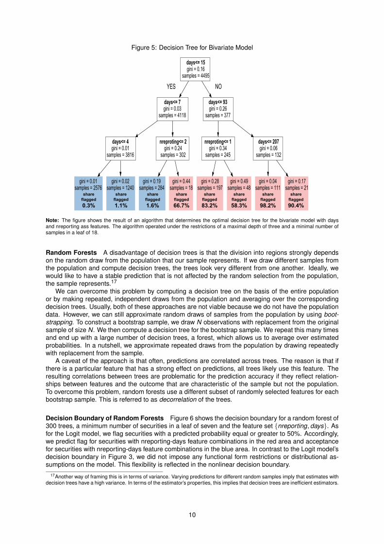
Figure 5: Decision Tree for Bivariate Model

Note: The figure shows the result of an algorithm that determines the optimal decision tree for the bivariate model with daysand nreporting ass features. The algorithm operated under the restrictions of a maximal depth of three and a minimal number ofsamples in a leaf of 18.

Random Forests A disadvantage of decision trees is that the division into regions strongly dependson the random draw from the population that our sample represents. If we draw different samples fromthe population and compute decision trees, the trees look very different from one another. Ideally, wewould like to have a stable prediction that is not affected by the random selection from the population,the sample represents.17

We can overcome this problem by computing a decision tree on the basis of the entire populationor by making repeated, independent draws from the population and averaging over the correspondingdecision trees. Usually, both of these approaches are not viable because we do not have the populationdata. However, we can still approximate random draws of samples from the population by using boot-strapping. To construct a bootstrap sample, we draw N observations with replacement from the originalsample of size N. We then compute a decision tree for the bootstrap sample. We repeat this many timesand end up with a large number of decision trees, a forest, which allows us to average over estimatedprobabilities. In a nutshell, we approximate repeated draws from the population by drawing repeatedlywith replacement from the sample.

A caveat of the approach is that often, predictions are correlated across trees. The reason is that ifthere is a particular feature that has a strong effect on predictions, all trees likely use this feature. Theresulting correlations between trees are problematic for the prediction accuracy if they reflect relation-ships between features and the outcome that are characteristic of the sample but not the population.To overcome this problem, random forests use a different subset of randomly selected features for eachbootstrap sample. This is referred to as decorrelation of the trees.

Decision Boundary of Random Forests Figure 6 shows the decision boundary for a random forest of300 trees, a minimum number of securities in a leaf of seven and the feature set {nreporting, days}. Asfor the Logit model, we flag securities with a predicted probability equal or greater to 50%. Accordingly,we predict flag for securities with nreporting-days feature combinations in the red area and acceptancefor securities with nreporting-days feature combinations in the blue area. In contrast to the Logit model’sdecision boundary in Figure 3, we did not impose any functional form restrictions or distributional as-sumptions on the model. This flexibility is reflected in the nonlinear decision boundary.

17Another way of framing this is in terms of variance. Varying predictions for different random samples imply that estimates withdecision trees have a high variance. In terms of the estimator’s properties, this implies that decision trees are inefficient estimators.

10

Figure 6: Random Forest and Decision Boundary

Note: The figure shows an illustration of the decision boundary (solid line) resulting from bivariate classification with a randomforest. The blue (red) data points represent accepted (flagged) securities. For securities with a days-nreporting combination in thelight red (blue) area, we predict a flag (acceptance).

Strengths and Weaknesses of Models Without Structural Assumptions Conceptually, the ap-proach is very different from starting with structural assumptions on the relationship between the featuresand the outcome. Because there are no functional form restrictions that constrain the relationship be-tween features and the probability of a flag, the algorithm can flexibly portray interdependencies andnon-linearities in the data. Nonlinear and complex links between features and the outcome do not clashwith rigid assumptions on linearity, separability and the shape of the transformation function. Becauseof this flexibility, the approach is a very direct representation of the conditional probability in eq. (1). Thenonlinear decision boundary that results from the random forest in Figure 3 illustrates this flexibility.

The weaknesses of the approach are twofold. First, there is a tradeoff between the gain in flexibilityand the accuracy of predictions when we apply models without structural assumptions to high dimen-sional (large number of features) data. Following the law of large numbers (LLN), sample averagesconverge to expected values with an increasing number of observations in the sample. Because weget convergence to population parameters only if the number of observations underlying the predictiontends to infinity (LLN), the accuracy of predictions based on the premise of non-structural models (eq.(8)) decreases exponentially with an increasing number of features. This is because in eq. (8), the num-ber of observations underlying a prediction is the number of observations with similar feature values.If the number of features increases, the number of observations with similar feature values decreasesexponentially. Intuitively, whereas we might find securities with the same number of days since the ma-turity date, it is unlikely that we find a security with the same number of days, number of reporting banks,maturity, and security type. This is often called the curse of dimensionality. In contrast, in the struc-tural Logit model, our assumptions on the functional form of the relationship between features and theoutcome allow us to use the entire sample to estimate model parameters. Because we do not rely ona subset with the same feature values, our estimates allow for accurate predictions even if a particularcombination of feature values in x is not common in the sample.

Second, with higher flexibility, we run the risk of fitting the model too closely to the data, i.e. overfittingthe model. In case of overfitting, our model picks up relationships between features and the outcomethat are characteristic of the random sample but not the population. Picking up such sample-specificrelationships makes for low accuracy in out-of-sample predictions.18

18Overfitting can affect both, the Logit model and the random forest. However, due to its higher flexibility, there is more potentialfor overfitting of the random forest algorithm. For both models, there are ways to prevent overfitting. A first line of defence againstthe risk of overfitting is to judge the models with respect to the accuracy of out-of-sample predictions. For the Logit, a secondline of defence is regularization. In a nutshell, with regularization, we add a penalty term to the Likelihood function. The termpenalizes large parameter estimates and thereby provides a counter weight to the increase in the likelihood function, we achieveby overfitting (e.g., by adding additional features to the model or overestimating the size of coefficients). To include a penalty termin the individual Likelihood function in Footnote 8, we expand L by adding –λβ′β, the sum of squared parameter estimates. By

11

4 Results and External Validity

To compare the Logit model to the random forest, we evaluate the accuracy of both models’ out-of-sample predictions.19 A simple and straightforward method to assess out-of-sample prediction accuracyis cross-validation with the validation set approach. In the first step, we randomly split the securities intoa training dataset and a validation dataset and fit the models to the training data. In the second step,we make out-of-sample predictions for securities in the validation dataset on the basis of the first-stageestimates. We then compare the accuracy of both models’ predictions in terms of two metrics: recalland precision. Recall is formally defined as:

R =Tp

Tp + Fn, (10)

where Tp is the number of true positives (the number of flagged securities for which we correctly pre-dicted flags) and Fn is the number of false negatives (the number of flagged securities for which weincorrectly predicted acceptance). The nominator of eq. (10) equals the number of correctly predictedflags and the denominator equals the actual number of flags in the validation dataset. Taken together, Ris the share of flags in the validation dataset that were correctly predicted. Precision is formally definedas:

P =Tp

Tp + Fp, (11)

where Fp is the number of false positives (the number of accepted securities for which we incorrectlypredicted a flag). The nominator of eq. (11) equals the number of correctly predicted flags, whereas thedenominator equals the overall number of predicted flags. Intuitively, P measures the share of securitiesfor which we predicted a flag that were actually flagged.

The results of the validation set approach rest on a single random split of the data into a trainingdataset and a validation dataset. Therefore, the values of our performance metrics depend on therandom nature of the split. To overcome this problem, we implement stratified k-fold cross-validation. Instratified k-fold cross-validation, we randomly split the data into k equal sized datasets. To make surethat the number of flags is the same in each of these datasets, we stratify the sample by our outcomevariable. We then, in turn, use each of the k datasets as training data, computing the recall and precisionmetric for out-of-sample predictions in the other k – 1 datasets. This provides us with k values for recalland precision, each representing an estimation with a different randomly selected training dataset. Byaveraging over these k -values, we get average values for recall and precision that are stable in the senseof not depending on a single random split.

Table 1: Prediction accuracy

Logit Random ForestRegression Algorithm

Recall 0.63 0.86Precision 0.85 0.89

Note: The table shows average recall and precision with stratified five-fold cross-validation for the Logistic regression and therandom forest algorithm. Each of the algorithms uses the feature set that minimizes average recall.

Table 1 shows average recall and precision with stratified five-fold cross-validation for the Logisticregression and the random forest algorithm. For each method, we use the feature set that maximizesthe model’s performance in terms of recall.20

choosing λ, we can calibrate the size of the penalty. For the random forest, a strategy that is equivalent to regularization is limitingthe maximum number of splits (depth of decision trees). This prevents the algorithm from producing regions with few observationsand low out-of-sample prediction accuracy.

19We implement both models with the sklearn package in python.20For the random forest, we use the feature set {days, nreporting, mvalue, stype}, where stype is a set of dummy variables for

the instrument type. The Logistic regression uses the same set of features except for the nominal value. For the random forestalgorithm, we compute 300 trees and implement a maximum depth of six, again to maximize recall.

12

We find that both models have a similar performance in terms of precision. In terms of recall, therandom forest algorithm (R = 0.86) yields a 37% percent improvement over the Logistic regression(R = 0.63). Predicting flags with the random forest algorithm, we correctly identify 86% of the securitiesthat were flagged by compilers.

So far, we have treated human decisions as the benchmark for the algorithms. However, there is amargin for decision errors by compilers. If the compilers make random errors in their assessment, anideal algorithm should produce a non-zero share of false positives and negatives. Following this line ofreasoning, the algorithms can yield results that are superior to a human decision maker by filtering outrandom decision errors.21

In order to establish the external validity of our results, we predict two further types of measurementerrors using Logit regressions and random forests. The first type of errors concerns erroneous reportingof securities before the emission date. The second type of errors concerns missing reference data. Inboth cases, we get results that are similar to our findings in Section 4.22

5 Implementation

Because of its higher out-of-sample accuracy, we focus on the implementation of the random forestalgorithm. To implement the algorithm, we use all 4.495 reported securities and compiler decisionsas training data. We then predict the probabilities of flags for newly reported securities and add thepredictions to the data table, compilers use to evaluate securities for measurement errors. Figure 7shows an illustration of the data table with predicted probabilities for securities that were reported inOctober, 2016. Securities with a high predicted probability of a flag appear on the top of the table. Theconditional formatting allows compilers to easily spot potentially problematic securities. By providingcompilers with the predicted probability instead of making binary predictions of flags, we take advantageof all the information, the machine learning algorithm provides.

Figure 7: Result of additional out-of-sample predictions

Note: The figure shows the data table after an implementation of the random forest algorithm. The predicted probabilities areshown in the last column. The other columns show the isin that identifies the security and the features of the security (not in thefigure).

The sorting of securities by predicted probabilities of measurement errors increases the efficiencyof the DQM process. Because compilers know which securities are likely subject to a measurementerror, they can allocate their time more efficiently to these securities. The ordering furthermore leadsto a higher effectiveness of the evaluation process. Because the attention of compilers and their abil-ity to evaluate a security correctly decreases with each security they review, checking securities witha high probability of a measurement error first increases the success of compilers’ efforts to identifymeasurement errors in the data.

21Of course, if decision errors are structural, the algorithm might learn to make the same mistakes as the compiler.22For securities that were reported before their emission date, predictions of flags with the random forest algorithm achieve a

recall of 77% and a precision of 88%. Predictions with Logit regression yield a recall of 50% and a precision of 86%. Regardingthe attribution of a lack of reference data to a measurement error, predictions with the random forest algorithm have a recall of96% and a precision of 97%. The Logit regression produces predictions with a recall of 39% and a precision of 97%.

13

Figure 8: Result of additional out-of-sample predictions

flagged accepted0.00

0.25

0.50

0.75

1.00n=28 n=799

Classificationflagged

weakly flagged

weakly accepted

accepted

Note: The figure shows the result of additional out-of-sample predictions for securities reported in October, 2016. The left (right)bar shows securities that were flagged (accepted) by compilers. The colours correspond to the predicted probabilities.

Figure 8 shows the results of out-of-sample predictions for the securities that were reported in Oc-tober, 2016 and were not part of the training dataset.23 The left (right) bar shows securities that wereflagged (accepted) by compilers. We find that the algorithm classifies more than 85% of securities thatwere flagged by compilers as weakly flagged or flagged. If we had informed compilers about the classi-fication, they would have found all of the 28 flagged securities in the top-35 of the list of 827 securitieswhich they received for evaluation.

6 Using Machine Learning to Close Data Gaps

To illustrate that the potential of machine learning for official statistics is not limited to DQM, we evaluatethe possibility of using predictions with machine learning algorithms to close data gaps. Essentially,there are two prerequisites for the algorithms’ ability to close data gaps with out-of-sample predictionsof the missing values. First, there have to be dependencies between the outcome variable that suffersfrom data gaps and other features of a data point. Second, we have to observe some data points forwhich the outcome is not missing. In a nutshell, by learning about the dependencies between featuresand the outcome from data points where the outcome values are not missing, the algorithm can predictthe missing values.

To evaluate the success of the algorithms in closing data gaps, we use simulated data. By simulatingdata, we can vary the environments in which we evaluate the algorithms’ performance in a controlledfashion. For simplicity, we simulate a binary outcome variable yi ∈ {0, 1} with data gaps. The binaryvariable allows us to use the same performance metrics as in the DQM application. Intuitively, recall andprecision measure the success of the algorithm in predicting the missing values, i.e. the share of obser-vations with data gaps for which the prediction equals the unobserved value. While recall measures oursuccess in predicting the missing outcome yi = 1, precisions shows the performance of the algorithmsin predicting the missing outcome yi = 0.

In our simulations, we cover predictions in a wide range of datasets with different: binomial distri-butions (shares of data points with yi = 1), numbers of data points, data quality, degrees of correlationbetween data points, and nonlinear feature-outcome relationships. The simulations show that the ap-plication of machine learning to close data gaps has a large potential in many environments.24 If theoutcome variable measures occurrences of a rare event, the performance of the models suffers but

23If manual checks by compilers are replaced by predictions with a machine learning algorithm, problems can arise whenstructural changes in the data occur. Because the algorithm draws on historic training data, there might be no possibility tolearn about new ways in which a human decision maker would evaluate the data. To investigate whether this is a problem inour implementation, we evaluate whether predictions for October, 2016 on the basis of training data from more recent monthsare superior to predictions using older training data. We find no systematic difference in performance and conclude that therelationships between the outcome and features in our application are stable over time. Figure A.2 in the Appendix summarizesthe results of the analysis.

24For a detailed description of the simulation results, see section C of the Appendix.

14

can be improved by collecting larger datasets. Whereas correlated observations have a minor effect onperformance, data quality has a large positive effect on recall and precision. When we introduce non-linear feature-outcome relationships, the random forest algorithm is clearly superior to the Logit model.Taken together, the results show that machine learning algorithms have applications beyond DQM. Inparticular, they can be tested against other algorithms for the imputation of missing values to close datagaps.

7 Conclusion

There is a large potential to improve Data Quality Management if data on human decisions to flagobservations as erroneous is available. With data on decisions, supervised learning algorithms canapproximate the result of the human decision making process and predict probabilities of measurementerrors. We showed that, for data on German securities holdings, out-of-sample predictions using arandom forest algorithm are superior to predictions with the Logit model. The predicted probabilitiesallow for a prioritization in the DQM process and an increase in the effectiveness and efficiency of thesearch for measurement errors.

The application of machine learning to close data gaps illustrates that the potential of the methodsfor officieal statistics is not limited to DQM. Simulations show that the Logit model and the RandomForest accurately predict missing data over a wide range of datasets, with a superior performance of therandom forest algorithm in datasets with complex feature-outcome relationships. These findings suggestthat machine learning algorithms provide a powerful alternative to established imputation methods.

Future research on the application of machine learning to DQM could discuss unsupervised learningalgorithms. Unsupervised learning algorithms can help to identify measurement errors if no informationon human classifications of observations as erroneous is available.

15

References

AMANN, M., BALTZER, M. and SCHRAPE, M. (2012). Microdatabase: Securities holdings statistics aflexible multi-dimensional approach for providing user-targeted securities holdings data. Bundesbanktechnical documentation.

ANGRIST, J. and PISCHKE, J.-S. (2009). Mostly Harmless Econometrics: An Empiricist’s Companion.1st edn.

BATINI, C., CAPPIELLO, C., FRANCALANCI, C. and MAURINO, A. (2009). Methodologies for data qualityassessment and improvement. ACM computing surveys (CSUR), 41 (3), 16.

BATISTA, G. E. and MONARD, M. C. (2003). An analysis of four missing data treatment methods forsupervised learning. Applied Artificial Intelligence, 17 (5-6), 519–533.

FRIEDMAN, J., HASTIE, T. and TIBSHIRANI, R. (2001). The Elements of Statistical Learning, vol. 1.Springer Series in Statistics, Berlin.

JEREZ, J. M., MOLINA, I., GARCIA-LAENCINA, P. J., ALBA, E., RIBELLES, N., MARTIN, M. and FRANCO,L. (2010). Missing data imputation using statistical and machine learning methods in a real breastcancer problem. Artificial Intelligence in Medicine, 50 (2), 105–115.

TOMZ, M., KING, G. and ZENG, L. (2003). Relogit: Rare events logistic regression. Journal of StatisticalSoftware, 8 (i02).

16

Appendix

A Figures

Figure A.1: Decision Tree and Decision Boundary

0 20 40 60

days

0

20

40

60

nreporting

decision boundary

accepted

flagged

Note: The figure shows an illustration of the bivariate decision tree’s decision boundary (solid line). The blue (red) data pointsrepresent accepted (flagged) securities. For securities with a days-nreporting combination in the red (blue) area, we predict a flag(acceptance).

Figure A.2: Decision Tree and Decision Boundary

Feb Mar Apr May Jun Jul Aug

training data

0.00

0.25

0.50

0.75

1.00

recall

Feb Mar Apr May Jun Jul Aug

training data

0.00

0.25

0.50

0.75

1.00

precision

Note: The figure shows the performance of the random forest algorithm in terms of recall (left panel) and precision (right panel) forout-of-sample predictions of measurement errors in securities data, reported in October, 2016. To evaluate a potential influenceof the time lag between the collection of the training data and the reporting date of the data for which we make predictions, we usetraining data from different months. For the first bar of each panel, for example, we only use data from February, 2016 as trainingdata. The figure shows no indication of a systematic negative relationship between the time lag and performance. The dashedlines show the mean recall and precision.

17

B Derivation of the Logit Model

From an econometric perspective, we can derive the Logit model from a decision model, if we interpretthe index function (2) as a latent score that the compiler uses to decide whether to flag security i . Westart by assuming that there is an additive, logistically distributed decision error ui . Then, we get thelatent score:

z∗i = α + xTi β + ui .

If the compiler flags security i for z∗i > 0 and accepts the security otherwise, we get:

P(yi = 1|xi

)= P

(z∗i > 0|xi

)= P

(ui > –xT

i β|xi)

= 1 – P(ui ≤ –xT

i β|xi)

Because we assumed that ui is logistically distributed, the conditional probability P(ui ≤ –xT

i β|xi)

is thedensity of the cumulative logistic distribution function Λ(·) (sigmoid function) at –xT

i β. Hence, we get:

1 – P(ui ≤ –xT

i β|xi)

= 1 – Λ(

– xTi β).

Because of the symmetry of the sigmoid function, this reduces to:

1 – Λ(

– xTi β)

= Λ(xT

i β)

= Λ(zi).

In sum, we have shown that P(yi = 1|xi

)= Λ(zi)

if decisions are based on a latent score with an additivedecision error that is drawn from the logistic distribution. In Machine Learning, we put no emphasis onthe decision model underlying the Logit but focus on the ability of the model to provide a good fit to thedata.

18

C Using Machine Learning to Close Data Gaps: Simulations

We proceed in two steps to simulate a dataset. First, for each of N data points, we randomly draw afeature value xi from the normal distribution N (µ,σ2) and an unobserved element ei from the logisticdistribution L(µ, s). Second, we determine the outcome for each data point with the univariate model:

yi =

{0 for α + γxi + ei < 01 for α + γxi + ei ≥ 0

. (1)

We end up with a simulated dataset with data points for which yi = 1 and data points for which yi = 0.By constructing the outcome with eq. (1), we implement a structure in the data that the algorithms canlearn to predict the outcome.

After constructing a simulated dataset, we evaluate the algorithms’ performance in terms of precisionand recall using stratified five-fold cross-validation. In the cross-validation procedure, we make out-of-sample predictions for a randomly chosen subset of observations. Essentially, we treat the outcome ofthe subset as a data gap and fill this gap with the algorithm’s predictions. In constructing the performancemetrics, we evaluate the success of the algorithms in predicting the missing values, i.e. the share ofobservations with data gaps for which the prediction equals the unobserved value.

Because the performance metrics also depend on our random draws of x and e, we repeatedly:draw features and unobserved elements, construct a simulated dataset, implement the algorithms, andcalculate the performance metrics. This provides us with distributions of the precision and the recallmetric.

C.1 Benchmark: Linking the Simulation Results for Data Gaps to the Predictionof Measurement Errors

Simulating a binary variable with data gaps allows us to draw additional conclusions about the perfor-mance of machine learning algorithms in the application to measurement errors. This is because wecan interpret simulated data points with yi = 1 as “flagged” and simulated data points with yi = 0 as“accepted” observations.

To facilitate drawing conclusions about the performance of machine learning in DQM from the simula-tion results, we include a simulated dataset with characteristics that are common in the DQM applicationas a benchmark and show performance in the benchmark (grey dotted lines) in the Figures C.2, C.3,C.4, and C.6.25 To mirror the fact that measurement errors are a relatively rare event in most datasets,we choose the distributions of x and e and the parameter values in eq. (1) in the benchmark such thatthe average share of flagged data points is small (15%).26 Furthermore, human evaluations are usuallycontingent on a pre-selection of data points from the original dataset. We conjecture that because ofthis pre-selection, the number of data points is likely in the lower four-digit range and choose N = 2 000as the number of data points in our benchmark.27

Figure C.1 illustrates the recall and precision of predictions for the benchmark simulations. Theleft panel shows that the median recall is similar for both models. The right panel indicates that theLogit model is slightly superior in terms of precision. Overall, the random forests’ performance is moredisperse.

The improvement of the Logit model’s performance for the simulated data compared to the applicationto German securities holdings data is due to the simulated data generating process closely following theLogit’s modelling assumptions.

25In Figure C.6, the benchmark performance is the performance at the intercept.26In eq. (1), we set alpha to –1.09 and γ to one. For the distributions, we choose x ∼ N (µ = 0,σ2 = 1) and e ∼ L(µ = 0, s =

0.17). The scale parameter of s = 0.17 corresponds to a variance of 0.1. We implement a lower variance for the unobservableelement than for the feature in order to give the algorithms a better chance to approximate the result of the simulated decisionmaking process. For a detailed discussion of the performance of the algorithms in environments with a higher variance of theunobservable element, see Section C.4.

27We provide an evaluation of the algorithms for different numbers of data points in Section C.3.

19

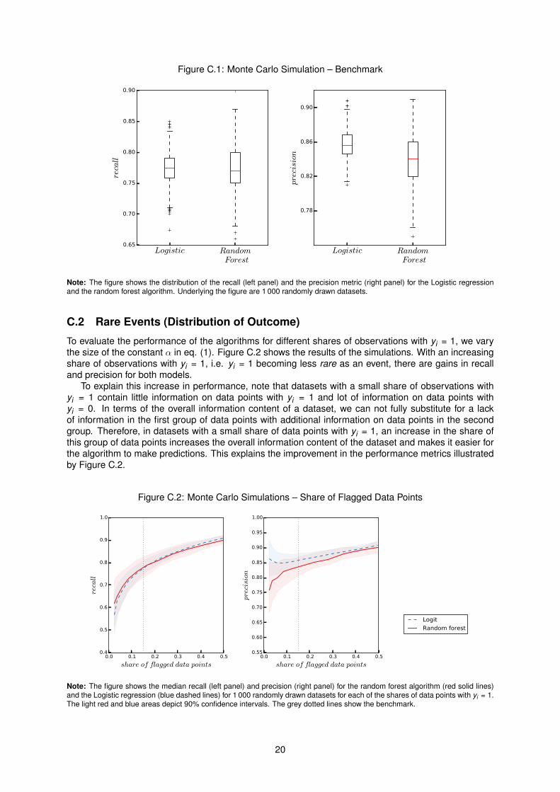
Figure C.1: Monte Carlo Simulation – Benchmark

Logistic Random Forest

0.65

0.70

0.75

0.80

0.85

0.90

recall

Logistic Random Forest

0.78

0.82

0.86

0.90

precision

Note: The figure shows the distribution of the recall (left panel) and the precision metric (right panel) for the Logistic regressionand the random forest algorithm. Underlying the figure are 1 000 randomly drawn datasets.

C.2 Rare Events (Distribution of Outcome)

To evaluate the performance of the algorithms for different shares of observations with yi = 1, we varythe size of the constant α in eq. (1). Figure C.2 shows the results of the simulations. With an increasingshare of observations with yi = 1, i.e. yi = 1 becoming less rare as an event, there are gains in recalland precision for both models.

To explain this increase in performance, note that datasets with a small share of observations withyi = 1 contain little information on data points with yi = 1 and lot of information on data points withyi = 0. In terms of the overall information content of a dataset, we can not fully substitute for a lackof information in the first group of data points with additional information on data points in the secondgroup. Therefore, in datasets with a small share of data points with yi = 1, an increase in the share ofthis group of data points increases the overall information content of the dataset and makes it easier forthe algorithm to make predictions. This explains the improvement in the performance metrics illustratedby Figure C.2.

Figure C.2: Monte Carlo Simulations – Share of Flagged Data Points

0.0 0.1 0.2 0.3 0.4 0.5

share of flagged data points

0.4

0.5

0.6

0.7

0.8

0.9

1.0

recall

0.0 0.1 0.2 0.3 0.4 0.5

share of flagged data points

0.55

0.60

0.65

0.70

0.75

0.80

0.85

0.90

0.95

1.00

precision

Logit

Random forest

Note: The figure shows the median recall (left panel) and precision (right panel) for the random forest algorithm (red solid lines)and the Logistic regression (blue dashed lines) for 1 000 randomly drawn datasets for each of the shares of data points with yi = 1.The light red and blue areas depict 90% confidence intervals. The grey dotted lines show the benchmark.

20

C.3 Number of Data Points

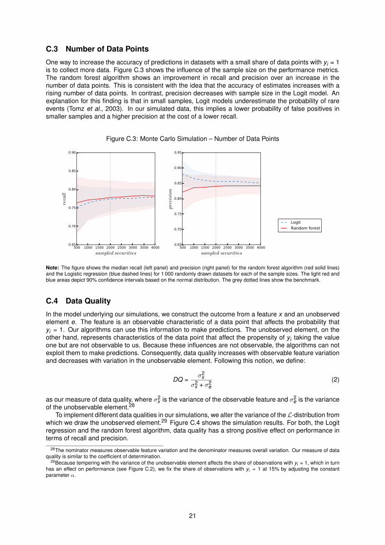
One way to increase the accuracy of predictions in datasets with a small share of data points with yi = 1is to collect more data. Figure C.3 shows the influence of the sample size on the performance metrics.The random forest algorithm shows an improvement in recall and precision over an increase in thenumber of data points. This is consistent with the idea that the accuracy of estimates increases with arising number of data points. In contrast, precision decreases with sample size in the Logit model. Anexplanation for this finding is that in small samples, Logit models underestimate the probability of rareevents (Tomz et al., 2003). In our simulated data, this implies a lower probability of false positives insmaller samples and a higher precision at the cost of a lower recall.

Figure C.3: Monte Carlo Simulation – Number of Data Points

500 1000 1500 2000 2500 3000 3500 4000

sampled securities

0.65

0.70

0.75

0.80

0.85

0.90

recall

500 1000 1500 2000 2500 3000 3500 4000

sampled securities

0.65

0.70

0.75

0.80

0.85

0.90

0.95

precision

Logit

Random forest

Note: The figure shows the median recall (left panel) and precision (right panel) for the random forest algorithm (red solid lines)and the Logistic regression (blue dashed lines) for 1 000 randomly drawn datasets for each of the sample sizes. The light red andblue areas depict 90% confidence intervals based on the normal distribution. The grey dotted lines show the benchmark.

C.4 Data Quality

In the model underlying our simulations, we construct the outcome from a feature x and an unobservedelement e. The feature is an observable characteristic of a data point that affects the probability thatyi = 1. Our algorithms can use this information to make predictions. The unobserved element, on theother hand, represents characteristics of the data point that affect the propensity of yi taking the valueone but are not observable to us. Because these influences are not observable, the algorithms can notexploit them to make predictions. Consequently, data quality increases with observable feature variationand decreases with variation in the unobservable element. Following this notion, we define:

DQ =σ2

xσ2

x + σ2e

(2)

as our measure of data quality, where σ2x is the variance of the observable feature and σ2

e is the varianceof the unobservable element.28

To implement different data qualities in our simulations, we alter the variance of the L-distribution fromwhich we draw the unobserved element.29 Figure C.4 shows the simulation results. For both, the Logitregression and the random forest algorithm, data quality has a strong positive effect on performance interms of recall and precision.

28The nominator measures observable feature variation and the denominator measures overall variation. Our measure of dataquality is similar to the coefficient of determination.

29Because tempering with the variance of the unobservable element affects the share of observations with yi = 1, which in turnhas an effect on performance (see Figure C.2), we fix the share of observations with yi = 1 at 15% by adjusting the constantparameter α.

21

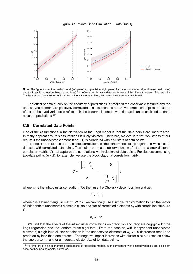
Figure C.4: Monte Carlo Simulation – Data Quality

0.5 0.6 0.7 0.8 0.9

Data Quality

0.2

0.3

0.4

0.5

0.6

0.7

0.8

0.9recall

0.5 0.6 0.7 0.8 0.9

Data Quality

0.55

0.60

0.65

0.70

0.75

0.80

0.85

0.90

0.95

precision

Logit

Random forest

Note: The figure shows the median recall (left panel) and precision (right panel) for the random forest algorithm (red solid lines)and the Logistic regression (blue dashed lines) for 1 000 randomly drawn datasets for each of the different degrees of data quality.The light red and blue areas depict 90% confidence intervals. The grey dotted lines show the benchmark.

The effect of data quality on the accuracy of predictions is smaller if the observable features and theunobserved element are positively correlated. This is because a positive correlation implies that someof the unobserved variation is reflected in the observable feature variation and can be exploited to makeaccurate predictions.30

C.5 Correlated Data Points

One of the assumptions in the derivation of the Logit model is that the data points are uncorrelated.In many applications, this assumptions is likely violated. Therefore, we evaluate the robustness of ourresults if the unobserved element in eq. (1) is correlated within clusters of data points.

To assess the influence of intra-cluster correlations on the performance of the algorithms, we simulatedatasets with correlated data points. To simulate correlated observations, we first set up a block diagonalcorrelation matrix (C) that captures the correlations within clusters of data points. For clusters comprisingtwo-data points (n = 2), for example, we use the block-diagonal correlation matrix:

C =

[1 ρcρc 1

]0

. . .

0[

1 ρcρc 1

] ,

where ρc is the intra-cluster correlation. We then use the Cholesky decomposition and get:

C = LLT ,

where L is a lower triangular matrix. With L, we can finally use a simple transformation to turn the vectorof independent unobserved elements e into a vector of correlated elements ec with correlation structureC:

ec = L*e.

We find that the effects of the intra-cluster correlations on prediction accuracy are negligible for theLogit regression and the random forest algorithm. From the baseline with independent unobservedelements, a high intra-cluster correlation in the unobserved elements of ρe = 0.9 decreases recall andprecision by less than one percent. The negative impact increases with cluster size but remains belowthe one percent mark for a moderate cluster size of ten data points.

30For inference in an econometric applications of regression models, such correlations with omitted variables are a problembecause they bias parameter estimates.

22

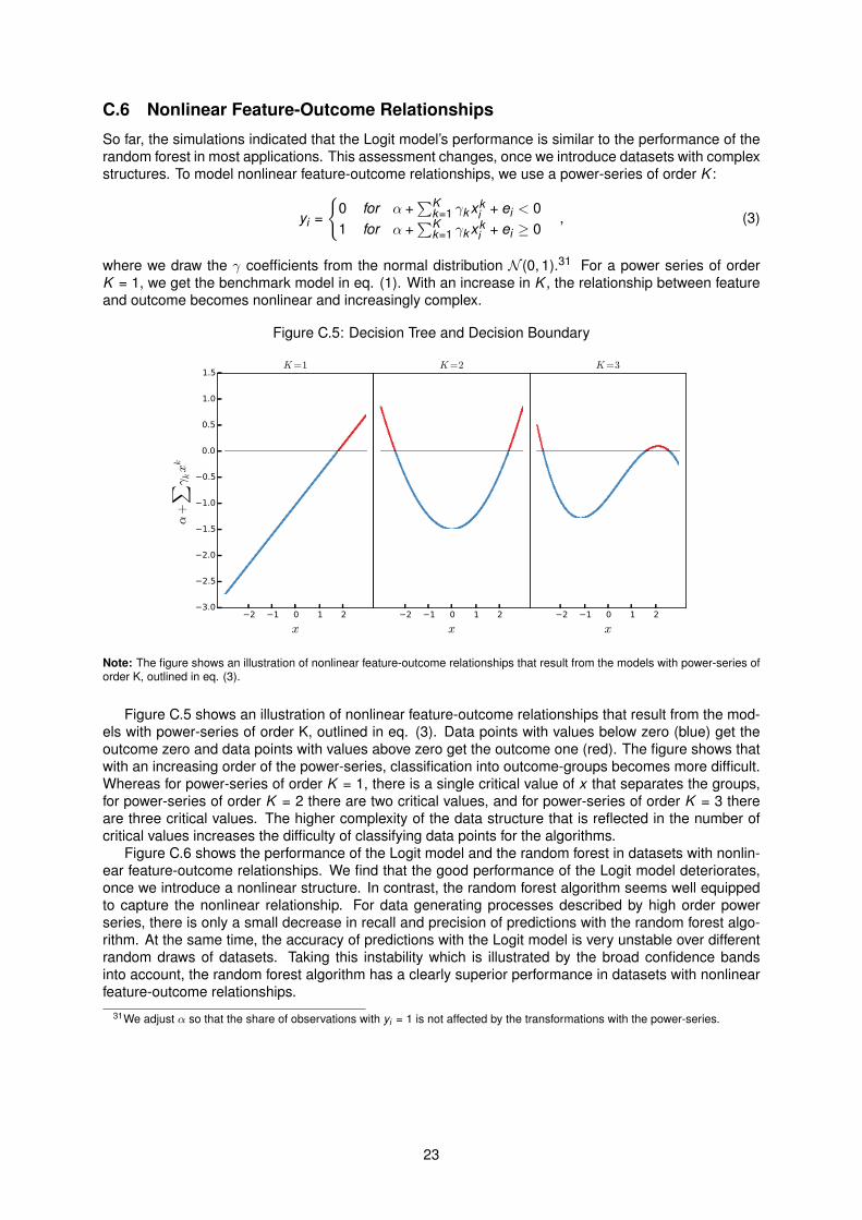
C.6 Nonlinear Feature-Outcome Relationships

So far, the simulations indicated that the Logit model’s performance is similar to the performance of therandom forest in most applications. This assessment changes, once we introduce datasets with complexstructures. To model nonlinear feature-outcome relationships, we use a power-series of order K :

yi =

{0 for α +

∑Kk=1 γk xk

i + ei < 01 for α +

∑Kk=1 γk xk

i + ei ≥ 0, (3)

where we draw the γ coefficients from the normal distribution N (0, 1).31 For a power series of orderK = 1, we get the benchmark model in eq. (1). With an increase in K , the relationship between featureand outcome becomes nonlinear and increasingly complex.

Figure C.5: Decision Tree and Decision Boundary

2 1 0 1 2

x

3.0

2.5

2.0

1.5

1.0

0.5

0.0

0.5

1.0

1.5

α+∑ γ

kxk

K=1

2 1 0 1 2

x

K=2

2 1 0 1 2

x

K=3

Note: The figure shows an illustration of nonlinear feature-outcome relationships that result from the models with power-series oforder K, outlined in eq. (3).

Figure C.5 shows an illustration of nonlinear feature-outcome relationships that result from the mod-els with power-series of order K, outlined in eq. (3). Data points with values below zero (blue) get theoutcome zero and data points with values above zero get the outcome one (red). The figure shows thatwith an increasing order of the power-series, classification into outcome-groups becomes more difficult.Whereas for power-series of order K = 1, there is a single critical value of x that separates the groups,for power-series of order K = 2 there are two critical values, and for power-series of order K = 3 thereare three critical values. The higher complexity of the data structure that is reflected in the number ofcritical values increases the difficulty of classifying data points for the algorithms.

Figure C.6 shows the performance of the Logit model and the random forest in datasets with nonlin-ear feature-outcome relationships. We find that the good performance of the Logit model deteriorates,once we introduce a nonlinear structure. In contrast, the random forest algorithm seems well equippedto capture the nonlinear relationship. For data generating processes described by high order powerseries, there is only a small decrease in recall and precision of predictions with the random forest algo-rithm. At the same time, the accuracy of predictions with the Logit model is very unstable over differentrandom draws of datasets. Taking this instability which is illustrated by the broad confidence bandsinto account, the random forest algorithm has a clearly superior performance in datasets with nonlinearfeature-outcome relationships.

31We adjust α so that the share of observations with yi = 1 is not affected by the transformations with the power-series.

23

Figure C.6: Monte Carlo Simulation – Nonlinear Feature-outcome Relationships

1 2 3 4

order of power series

0.25

0.50

0.75

1.00recall

1 2 3 4

order of power series

0.25

0.50

0.75

1.00

precision

Logit

Random forest

Note: The figure shows the median recall (left panel) and precision (right panel) for the random forest algorithm (red solid lines)and the Logistic regression (blue dashed lines) for 1 000 randomly drawn datasets for each of the orders of the power series. Thelight red and blue areas depict 90% confidence intervals. The grey dotted lines show the benchmark.

24