improving caravan design by modelling of crosswindeprints.usq.edu.au/31393/1/deleon_a_wandel.pdf ·...
TRANSCRIPT

University of Southern Queensland
Faculty of Health, Engineering and Sciences
Improving Caravan Design by Modelling of Crosswind
A dissertation submitted by
Mr Adrian De Leon
in fulfilment of the requirements of
Courses ENG4111 and ENG4112 Research Project
towards the degree of
Bachelor of Engineering (Mechanical Engineering)
Submitted October 2016

ii
ABSTRACT
It is a well-known fact that towing a caravan over long distances can be a very expensive
exercise especially with the rise in cost of fuel. Caravans by design are generally not seen
to exhibit any standout aerodynamic features and as such can increase the fuel
consumption of the tow vehicle by more than double. The effects of wind on the
aerodynamics of the caravan are also of importance. Of particular interest, the effect that
cross wind flow has on caravans is somewhat of an under stated issue. This project aims
to analyze the effect of crosswind flow, propose some caravan modifications and evaluate
any advantages to the tow vehicle regarding fuel economy.
The project aims to use Computational Fluid Dynamics to evaluate the caravan under a
variety of operating conditions. By conducting a parametric study into various design
features on the caravan it is possible to evaluate these proposal with CFD to obtain data
that can show the potential increases in efficiency and economy over the original baseline
design.
The results show that there are significant forces at play when analyzing crosswind flow
on the caravan. The results also show that by carrying out modifications to key areas such
as the gap between the car and caravan and also its general shape, there is potential for
significant gains to be made in reducing the drag forces at play and subsequently enhancing
the fuel economy of the tow vehicle. Results confirm that these forces can be reduced by
up to 18%.

iii
University of Southern Queensland
Faculty of Health, Engineering and Sciences
ENG4111/ENG4112 Research Project
LIMITATIONS OF USE
The Council of the University of Southern Queensland, its Faculty of Health,
Engineering & Sciences, and the staff of the University of Southern Queensland,
do not accept any responsibility for the truth, accuracy or completeness of material
contained within or associated with this dissertation.
Persons using all or any part of this material do so at their own risk, and not at the
risk of the Council of the University of Southern Queensland, its Faculty of Health,
Engineering & Sciences or the staff of the University of Southern Queensland.
This dissertation reports an educational exercise and has no purpose or validity
beyond this exercise. The sole purpose of the course pair entitled “Research
Project” is to contribute to the overall education within the student’s chosen degree
program. This document, the associated hardware, software, drawings, and other
material set out in the associated appendices should not be used for any other
purpose: if they are so used, it is entirely at the risk of the user.
iv
CERTIFICATION OF DISSERTATION
I certify that the ideas, designs, experimental work, results, analyses and
conclusions set out in this dissertation are entirely my own effort, except where
otherwise indicated and acknowledged.
I further certify that the work is original and has not been previously submitted for
assessment in any other course or institution, except where specifically stated.
Adrian De Leon
Student Number: 0050108437
________________________________
Signature
________________________________
Date

v
ACKNOWLEDGEMENTS
The author Adrian De Leon would like to give acknowledgement to the following people;
Firstly I would like to thank Dr Andrew Wandel, for his guidance and support throughout
this project. His assistance and dedication to supervising this project allowed me to gain a
greater understanding of Computational Fluid Dynamics. His expertise in ANSYS was
invaluable in order to bring all the research elements together.
Secondly, I would like to thank my family and in particular my wife Pamela for her support
throughout the past seven years of study, which culminate with the completion of this
research. Without her patience and support I would not have been able to come as far as I
have come in my academic life.

vi
TABLE OF CONTENTS
ABSTRACT ........................................................................................................... ii
LIMITATIONS OF USE ...................................................................................... iii
CERTIFICATION OF DISSERTATION ............................................................. iv
ACKNOWLEDGEMENTS ................................................................................... v
LIST OF FIGURES ............................................................................................... ix
LIST OF APPENDICES ...................................................................................... xii
NOMENCLATURE ............................................................................................ xiii
CHAPTER 1 - INTRODUCTION ......................................................................... 1
1.1 Background ............................................................................................. 1
1.2 Outline of the Study ................................................................................ 1
1.3 Research Aims and Objectives ................................................................ 2
1.4 Dissertation Outline ................................................................................ 3
1.4.1 Chapter 1 – Introduction ............................................................... 3
1.4.2 Chapter 2 – Literature Review ...................................................... 3
1.4.3 Chapter 3 – Research Methodology .............................................. 4
1.4.4 Chapter 4 – Pre-Optimization Study ............................................. 4
1.4.5 Chapter 5 – Parametric Study on Baseline Configuration ............ 4
1.4.6 Chapter 6 – Results & Discussions ............................................... 4
1.4.7 Chapter 7 – Conclusion ................................................................. 5
1.5 Consequential Effects .............................................................................. 5
1.5.1 Ethical Considerations .................................................................. 5
1.5.2 Risk Assessment ........................................................................... 6
1.6 Summary of Methodology ...................................................................... 6
1.7 Resources Requirements ......................................................................... 8
1.8 Project Timelines .................................................................................... 8
CHAPTER 2 – LITERATURE REVIEW ............................................................. 9
2.1 Introduction ............................................................................................. 9
2.2 Study of Aerodynamics ........................................................................... 9
2.3 Crosswind Aerodynamic Effects in Transportation Vehicles ............... 10
2.3.1 Cars ............................................................................................. 10
2.3.2 Rail Transportation ..................................................................... 12
2.3.3 Truck & Trailer ........................................................................... 15
2.4 Selection of Tow Vehicle for Study ...................................................... 17

vii
2.4.1 Tow Vehicle Characteristics ....................................................... 18
2.5 Caravan Development ........................................................................... 19
2.5.1 Caravan Classification ................................................................ 19
2.6 Computational Fluid Dynamics ............................................................ 22
2.7 Application of CFD to Vehicle Aerodynamics Analysis ...................... 22
2.8 Application of CFD to Caravan Analysis ............................................. 23
2.9 CFD Pre-Processing .............................................................................. 25
2.9.1 Development of Geometry .......................................................... 26
2.9.2 Mesh Generation ......................................................................... 26
2.9.3 Establishment of Boundary Conditions & Turbulence Models .. 27
2.10 CFD Solver ..................................................................................... 30
2.11 CFD Post Processing ........................................................................... 32
2.12 Force Coefficient Calculation ............................................................. 32
2.13 Literature Review Summary ............................................................... 33
CHAPTER 3 – RESEARCH METHODOLOGY ................................................ 34
3.1 Overview ............................................................................................... 34
3.2 Vehicle Selection ................................................................................... 34
3.3 Modelling Technique ............................................................................ 34
3.4 Vehicle Geometry ................................................................................. 36
3.5 Fluid Domain ......................................................................................... 38
3.6 3D Model Validation ............................................................................. 39
3.7 Mesh Setup ............................................................................................ 41
3.8 Global Mesh Sizing Control .................................................................. 41
3.8.1 Relevance and Relevance Center ................................................ 42
3.8.2 Advanced Size Function ............................................................. 42
3.8.3 Initial Mesh ................................................................................. 43
3.9 Grid Independence Study ...................................................................... 45
3.10 Enclosure Dimensioning ..................................................................... 47
3.11 Final Mesh Detail ................................................................................ 47
3.12 CFX Simulation Setup ........................................................................ 48
3.12.1 Fluid Model Configuration ....................................................... 48
3.12.2 Domain Initialisation ................................................................ 49
3.12.3 Boundary Setup ......................................................................... 49
3.12.4 Monitor Points .......................................................................... 53
3.12.5 Solver Control Setup ................................................................. 53

viii
3.12.6 Solution Component Setup ....................................................... 53
3.13 Caravan Selection ................................................................................ 54
3.13.1 Caravan Geometry .................................................................... 56
3.13.2 Caravan Meshing ...................................................................... 57
3.14 Caravan CFX Simulation .................................................................... 59
3.15 Summary of Results ............................................................................ 61
CHAPTER 4 – PRE-OPTIMIZATION STUDY ................................................. 62
4.1 Wind Loading Forces ............................................................................ 62
4.1.1 Drag Force in X Direction .......................................................... 63
4.1.2 Lift Force in Y Direction ............................................................ 64
4.1.3 Side Force in Z Direction ............................................................ 64
4.1.4 Flow Streamlines ........................................................................ 65
4.1.5 Pressure Distribution ................................................................... 67
4.1.6 Turbulence Kinetic Energy ......................................................... 68
CHAPTER 5 – PARAMETRIC STUDY ............................................................. 70
5.1 Overview ............................................................................................... 70
5.1.1 Car and Caravan Gap .................................................................. 70
5.1.2 Caravan Edge Profile .................................................................. 71
5.1.3 Caravan Frontal Vanes ............................................................ 72
CHAPTER 6 – RESULTS & DISCUSSION ....................................................... 74
6.1 Overview ............................................................................................... 74
6.2 Crosswind Coefficient Calculations ...................................................... 74
6.3 Geometry Variation ............................................................................... 80
6.3.1 Draw Bar Modification ............................................................... 80
6.3.2 Edge Radius Modification .......................................................... 82
6.3.3 Frontal Vane Modification .......................................................... 84
6.4 Fuel Efficiency Calculations ................................................................. 85
CHAPTER 7 - CONCLUSION ............................................................................ 86
7.1 Overview ............................................................................................... 86
7.2 Conclusions ........................................................................................... 86
7.3 Limitations and Future Work ................................................................ 87
LIST OF REFERENCES ..................................................................................... 88
APPENDICES ...................................................................................................... 91

ix
LIST OF FIGURES
Figure 1.1: Typical Twin Axle Caravan (Jayco, 2016) .......................................... 2
Figure 2.1: Crosswind Velocity Components (Mansor et al. 2013) ..................... 10
Figure 2.2: Model T Ford (Dorling Kindersley, 2016) ........................................ 11
Figure 2.3: La Jamais Contente (The Truth about Cars, 2016) ............................ 11
Figure 2.4: Crosswind related Train Accidents (Asress & Svorcan, 2014) ......... 13
Figure 2.5: 1830’s ‘Rocket’ Steam Locomotive & AGV Italo Bullet Train ........ 14
Figure 2.6: Truck Rollover Incident due to Crosswind (WILX News, 2014) ..... 15
Figure 2.7: Land Rover Discovery 4 (Without-a-Hitch, 2016) ............................ 17
Figure 2.8: Conventional Single Axle Caravan (Swift Group , 2016) ................. 19
Figure 2.9: Twin Axle Caravan (Jayco, 2016) ..................................................... 20
Figure 2.10: Pop Top Caravan (Jayco, 2016) ....................................................... 20
Figure 2.11: GRP Caravan (Jayco, 2016) ............................................................ 21
Figure 2.12: Camper Trailer (Jayco, 2016) .......................................................... 21
Figure 2.13: Fifth Wheeler (Grey Wolf, 2016) .................................................... 22
Figure 2.14: Wind Tunnel Test Setup (Autoevolution & NASA) ....................... 23
Figure 2.15: CFD Simulation-Flow Modelling (Glyndwr University, 2011) ...... 24
Figure 2.16: Near Wall Velocity CFD Study (Swift Group, 2013) ..................... 25
Figure 2.17: Flow regimes at the Wall Interface (Frei, 2013) .............................. 29
Figure 2.18: Residual Monitors ............................................................................ 31
Figure 2:19: Monitor of Point of Interest (Thoms, 2007) .................................... 31
Figure 3.1: Original Land Rover Model (Creo Parametric) ................................ 35
Figure 3.2: Simplified Land Rover Model (Creo Parametric) ............................. 36
Figure 3.3: Model imported into ANSYS. ........................................................... 37
Figure 3.4: Non Uniform Enclosure ..................................................................... 38
Figure 3.5: Drag Force in X and Z directions on Vehicle .................................... 40
Figure 3.6: ASF Meshing Comparison (Leap Australia, 2011) ........................... 43
Figure 3.7: Proximity and Curvature ASF mesh detail ........................................ 43
Figure 3.8: Isometric View of Meshed Domain ................................................... 44
Figure 3.9: Detail View of Initial Vehicle Mesh .................................................. 45
Figure 3.10: Inlet Boundary CFX ........................................................................ 50
Figure 3.11: Outlet Boundary CFX ...................................................................... 50
Figure 3.12: Opening Boundary CFX .................................................................. 51
Figure 3.13: Road Boundary CFX ....................................................................... 52
Figure 3.14: Complete Boundary Setup CFX ...................................................... 52
Figure 3.15: Solver Run Settings ......................................................................... 54
Figure 3.16: Jayco Starcraft (Jayco, 2016) ........................................................... 55
Figure 3.17: Trackmaster Simpson (Trackmaster, 2016) ..................................... 55
Figure 3.18: Majestic Knight (Majestic Caravans, 2016) .................................... 56
Figure 3.19: Final Caravan Model ....................................................................... 57
Figure 3.20: Car & Caravan Model Mesh ............................................................ 58
Figure 3.21: Car Caravan Boundary Set Up at Zero Yaw ................................... 59
Figure 3.22: Force Monitors Graph for Baseline Caravan ................................... 60
Figure 3.23: Residuals-At convergence (Caravan Set Up) .................................. 60

x
Figure 4.1: Force in X Direction for Baseline Caravan ....................................... 63
Figure 4.2: Force in Y Direction for Baseline Caravan ....................................... 64
Figure 4.3: Force in Z Direction for Baseline Caravan ........................................ 65
Figure 4.4: Velocity Streamlines for Baseline Caravan ....................................... 65
Figure 4.5: Velocity Streamlines Baseline Caravan at 45° flow (1) .................... 66
Figure 4.6: Velocity Streamlines Baseline Caravan 45° flow (2) ........................ 66
Figure 4.7: Pressure Distribution for Baseline Caravan at 0° flow ...................... 67
Figure 4.8: Pressure Distribution for Baseline Caravan at 45° flow .................... 67
Figure 4.9: Turbulent Kinetic Energy for Baseline Caravan at 0° Yaw .............. 68
Figure 4.10: Turbulent Kinetic Energy for Baseline Caravan at 45° Yaw .......... 69
Figure 5.1: 100mm Caravan Edge Radius ........................................................... 71
Figure 5.2: 350mm Caravan Edge Radius ........................................................... 72
Figure 5.3: Caravan Frontal Vane Modification .................................................. 73
Figure 6.1: Drag Coefficients for Modified Caravan Draw Bar .......................... 76
Figure 6.2: Lift Coefficients for Modified Caravan Draw Bar ............................ 78
Figure 6.3: Side Force Coefficients for Modified Caravan Draw Bar ................. 80
Figure 6.4: Draw Bar Forces in x Direction ......................................................... 81
Figure 6.5: Draw Bar Forces in y Direction ......................................................... 81
Figure 6.6: Draw Bar Forces in z Direction ......................................................... 81
Figure 6.7: Pressure Distribution on Caravan with 1.0 m Draw Bar ................... 82
Figure 6.8: Baseline Caravan Edge Modification Comparison ............................ 83
Figure 6.9: 350mm Edge at 45° flow ................................................................... 84
Figure 6.10: Velocity Streamlines of Final Caravan Design ............................... 85
Figure K1: Residuals for Final Caravan Model with Vanes .............................. 103

xi
LIST OF TABLES
Table 1:Truck Power Consumption Figures (Patten et al. 2012) ......................... 16
Table 2: Turbulence Model Comparison (Frei, 2013) ......................................... 28
Table 3: Relevance ............................................................................................... 46
Table 4: Smoothing .............................................................................................. 46
Table 5: Transition Sizing .................................................................................... 46
Table 6: Span Angle Centre ................................................................................. 47
Table 7: Enclosure Dimensioning ........................................................................ 47
Table 8: Mesh Options ......................................................................................... 48
Table 9: Inlet Boundary Details ........................................................................... 49
Table 10: Outlet Boundary Details ....................................................................... 50
Table 11: Opening Boundary Details ................................................................... 51
Table 12: Road Boundary Details ........................................................................ 51
Table 13: Solver Control Details .......................................................................... 53
Table 14: Drag Coefficient for 1.8m Draw Bar ................................................... 74
Table 15: Drag Coefficients for 1.5m Draw Bar .................................................. 75
Table 16: Drag Coefficients for 1.0m Draw Bar .................................................. 75
Table 17: Lift Coefficient for 1.8m Draw Bar ..................................................... 76
Table 18: Lift Coefficient for 1.5m Draw Bar ..................................................... 77
Table 19: Lift Coefficient for 1.0m Draw Bar ..................................................... 77
Table 20: Side Force Coefficient for 1.8 m Draw Bar ......................................... 78
Table 21: Side Force Coefficients for 1.5m Draw Bar ........................................ 79
Table 22: Side Force Coefficients for 1.0m Draw Bar ........................................ 79
Table 23: Likelihood Category Table .................................................................. 93
Table 24: Consequence Category Table ............................................................... 94
Table 25: Risk Management Matrix (Australian Sports Commission) ................ 94
Table 26: Hazard 1 Risk Assessment ................................................................... 95
Table 27: Hazard 2 Risk Assessment ................................................................... 95
Table 28: Caravan 1.8m Draw Bar Data .............................................................. 97
Table 29: Caravan 1.5m Draw Bar Data .............................................................. 98
Table 30: Caravan 1.0m Draw Bar Data .............................................................. 99
Table 31: Caravan 1.8m Draw Bar with Modified Edge Data ........................... 100
Table 32: Caravan 1.5m Draw Bar with Modified Edge Data ........................... 101
Table 33: Caravan 1.0m Draw Bar with Modified Edge Data ........................... 102
Table 34: Frontal Vane System Data ................................................................. 103

xii
LIST OF APPENDICES
Appendix A - Project Specification .................................................................... 91
Appendix B - Project Timelines .......................................................................... 92
Appendix C - Risk Assessment ........................................................................... 93
Appendix D – Land Rover Specifications ........................................................... 96
Appendix E – Baseline Caravan Data Sheet (1.8 m Draw Bar) .......................... 97
Appendix F - Caravan 1.5 m Draw Bar Data Sheet ............................................ 98
Appendix G - Caravan 1.0 m Draw Bar Data Sheet ........................................... 99
Appendix H - Caravan 1.8m Draw Bar with Modified Edges .......................... 100
Appendix I - Caravan 1.5m Draw Bar with Modified Edges ............................ 101
Appendix J - Caravan 1.0m Draw Bar with Modified Edges ........................... 102
Appendix K - Baseline Caravan with Frontal Vane System ............................. 103

xiii
NOMENCLATURE
The following abbreviated terms have been utilized throughout this dissertation.
CFD Computational Fluid Dynamics
WH&S Work Health & Safety
km/h kilometres per Hour
N Newton’s
USQ University of Southern Queensland
m/s metres per second
SST Shear Stress Transport
F Aerodynamic Load
Cd Coefficient of Drag
v Velocity (m/s)
ρ Air Density (kg/m3)
A Frontal Area (m2)
GRP Glass Reinforced Plastic

1
CHAPTER 1 - INTRODUCTION
1.1 Background Recreational travel using caravans has been embraced by millions worldwide. The
industry has grown steadily since the mid to late 1950’s and the last two decades have seen
an exponential increase in technological advancement which has served to provide
travelers with a ‘home away from home’ which affords the ultimate in creature comforts
and flexibility.
Statistics on Recreational Vehicle (RV) usage within Australia as collected by the
Australian Bureau of Statistics (ABS) indicates that there are over half a million registered
recreational vehicles in use, with 90% of these categorized as caravans or towable camping
trailers.
Caravan design has evolved significantly throughout the decades. The focus on improving
aerodynamic efficiency has been at the top of many caravan design and manufacturer’s
priority lists. As caravan designs grow in size and complexity, the performance
characteristics of the towing vehicles have also had to improve in order to provide the
optimum capability to safely and efficiently tow these caravans.
Significant effort has been made to ensure a caravan’s shape and form is optimized to
provide maximum aerodynamic efficiency, in order to reduce the environmental and
economic impact due to the drag developed as it moves behind the tow vehicle, whilst also
ensuring maximum safety in relation to its dynamic stability under the influence of
external wind loads.
1.2 Outline of the Study
This study aims to expand on the research conducted by Briskey (2013) in which a tow
vehicle and caravan combination was evaluated using computational fluid dynamics
(CFD) practices. The study conducted by Briskey (2013) focused on the aerodynamic drag
produced by the caravan from a headwind perspective.
This study is primarily concerned with aerodynamic drag produced when the caravan is
subject to cross wind air flow and its subsequent effect on the fuel efficiency of the tow
vehicle. In addition, initial data gathered as part of this study will form part of an

2
optimization strategy for the baseline caravan configuration which will aim to reduce the
effects of aerodynamic drag on the caravan and enhance lateral stability.
This study will build on and explore the effects of cross wind aerodynamic loading on
moving vehicles as encountered throughout a literature review in which the majority of
literature focuses on vehicles such as cars, trucks and trains. The research will feature a
parametric study conducted on modifications to a baseline caravan geometry such as that
depicted in Figure 1, which will be assessed for their ability to reduce drag and therefore
make the caravan design more aerodynamically efficient and provide for improved safety
and handling.
Figure 1.1: Typical Twin Axle Caravan (Jayco, 2016)
1.3 Research Aims and Objectives
The original intent of the research was to utilise a caravan prototype developed by
Toowoomba based caravan manufacturer Airflow Caravans which was designed with
improved features which were intended to improve the fuel efficiency of the tow vehicle.
Unfortunately due to certain circumstances Airflow Caravans were not able to continue
providing in-kind support for this research. This required an additional task to identify a
suitable caravan and tow vehicle alternative for use in this study.
The project specification as detailed in Appendix A was therefore produced to outline the
deliverables of the research as an extension of the research conducted by Briskey (2013),
titled ‘Improving Caravan Design by Modelling of Airflow’. The project is broken down
into seven phases, with three additional phases to be conducted if time permits. The
objectives of the study are as follows:
1. Research the background information related to caravan drag profiles and towing
vehicle performance through CFD modeling.

3
2. Research geometry and performance data for subject caravan and tow vehicle.
3. Create a 3D model of the Caravan and Tow Vehicle for use in CFD analysis.
4. Validate 3D model using a headwind analysis.
5. Undertake CFD simulation of current prototype under cross wind conditions.
6. Investigate and propose performance enhancing modifications to the initial
baseline design.
7. Perform a CFD analysis and parametric study on the modified caravan.
If time permits the following tasks have been proposed in order to expand on the main
research conducted. They are as follows;
8. Propose further modifications.
9. Investigate the dynamic stability of the caravan and tow vehicle when subjected
to cross wind air flow.
10. Perform transient simulation of caravan/tow vehicle movement due to crosswind
loading.
1.4 Dissertation Outline
The following provides a general overview of each chapter of this dissertation.
1.4.1 Chapter 1 – Introduction
The structure of the dissertation is presented along with an introduction to the research
project. Background information relating to the selection of the problem, an outline of the
study and the research objectives are also documented. A summary of the project
methodology is provided along with consequential effects and risks associated with
undertaking this research.
1.4.2 Chapter 2 – Literature Review
This chapter presents a comprehensive literature review undertaken to understand the
scope of the research. Areas of literature reviewed and documented include; aerodynamics,

4
crosswind airflow effects on transportation vehicles and their optimization. Computational
Fluid Dynamics techniques and applicability to this study is also presented. This literature
review expands on the literature review conducted by Briskey (2013) in which the
influence of cross wind flow becomes the priority of this study.
1.4.3 Chapter 3 – Research Methodology
This chapter covers the methodology which is used to analyze the effect a crosswind will
have on the caravan/tow vehicle combination in terms of generating drag and other
aerodynamic forces. The process of generating a model to represent the vehicle geometry,
application of required meshing and the subsequent grid independence study is detailed in
addition to the setup parameters for the CFD analysis and pre-optimization solutions.
1.4.4 Chapter 4 – Pre-Optimization Study
This chapter presents the results of the baseline caravan/tow vehicle combination
configuration CFD study. Visual representations of airflow are presented and discussed in
detail. Recommendations are made to explore modifications that will be subsequently
evaluated in a post optimization parametric study.
1.4.5 Chapter 5 – Parametric Study on Baseline Configuration
This chapter details the optimization of the baseline model and details the method to
conduct a parametric study to produce new results that reflect the impact that the proposed
modifications have had in comparison to results detailed for the baseline configuration in
Chapter 4.
1.4.6 Chapter 6 – Results & Discussions
This chapter presents the results of the post optimization parametric study. It presents data
to present a comparison between pre and post modification results and provide both a
quantitative and qualitative assessment of the effectiveness of each featured modification.
This chapter also details further work and details issues encountered during the study and
potential for re-evaluation. Areas of research currently out of scope are detailed with any
improvement suggestions made to how the study can be conducted in future.

5
1.4.7 Chapter 7 – Conclusion
This chapter provides a summary of the outcome of the study and evaluates its success
against the project specification and original objectives. A final recommendation is
presented on a configuration that provides the greatest improvement in aerodynamic
efficiency and road handling. This chapter also details further work and details issues
encountered during the study and potential for re-evaluation. Areas of research currently
out of scope are detailed with any improvement suggestions made to how the study can be
conducted in future.
1.5 Consequential Effects
In order to provide an accurate assessment regarding the impact that this project will have
on the wider society currently involved in using caravans, it is important to understand
some of the important factors that affect customers experiences and expectations about the
topic.
These factors can be grouped into two main categories; sustainability and safety.
As a professional engineer, one is expected to make a conscientious effort to address these
two concerns amongst others in the pursuit of engineering excellence. Engineers Australia
(EA) has promoted its Code of Ethics in order to ensure that its members exercise their
responsibilities as professional engineers with due diligence and professionalism.
1.5.1 Ethical Considerations
Tenet 4 of the Code of Ethics relates to an Engineer’s responsibility to promote
sustainability (Engineers Australia, 2010).
The task involves research into the effects that drag has on a caravan/tow vehicle
combination and is focused on identifying the drag produced by crosswind flow, and how
this leads to higher operating costs through the increase in fuel consumption figures for
the tow vehicle. The effects of increased fossil fuel consumption are readily seen in the
environment through pollution and it is therefore seen as a major concern for engineers

6
that are concerned with offering consumers an option that is both financially viable for
them whilst also ensuring that any ill effects on the natural environment are minimized.
In addition, the safety of all persons utilizing the technology is to be a priority and a
conscientious effort is to be made to ensure that the engineering rigor applied to all phases
of the development is adequate to meet this objective.
1.5.2 Risk Assessment
The risks associated with both the conduct of this study and the research deliverables can
be separated into two distinct categories.
1. Risk associated with adopting recommendations and utilization of research data
from this dissertation as the basis of other research.
2. Risks and Hazards associated with the completing the research project in line with
WH&S principles
In addressing the first point, it is important to note that the research is to be conducted
utilizing available information captured at the time when the literature review was
conducted. Prior to implementing any recommendations an additional validation study is
to be conducted utilising scale model representations, tested in wind tunnels and where
possible extensive road testing to ensure that any anomalies in CFD findings are identified
and any areas of research outside of the scope of this task are addressed where required.
A risk assessment has been conducted and documented in Appendix C - Risk Assessment
for the risks associated with point 2 of this section.
1.6 Summary of Methodology
Detailing the methodology used in performing this study is a fundamental requirement in
order to give the research direction and to provide a roadmap to highlight the methods used
to obtain the deliverables as per the Project Specification.
Following the literature review phase, the project requires the creation of the models
required for the CFD simulation. The creation of the models can be performed utilizing
ANSYS Workbench or alternatively imported from a 3D modeling package such as Creo
Parametric or Autodesk Inventor Professional. Due to familiarity with the CREO modeling

7
package it has been selected as the software that will be used to model both the caravan
and tow vehicle geometry.
The models are then required to be examined against existing data to ensure that a
comparable result between published data, dimensioning and physical features exists. This
process will ensure that a relatively high level of confidence is achieved by using models
that accurately represent the actual product. This is achieved by ensuring that the
approximation of features used in the model do not significantly alter the aerodynamic
profile of the vehicle. In addition the mesh used is to be refined until the simulation results
don’t change significantly ensuring that numerical errors are as small as possible. For the
purpose of this study it has been decided that a value of no greater than 1 percent error is
acceptable in order to proceed with the CFD study. The caravan and tow vehicle models
are then combined to form the combination that will be evaluated in a headwind airflow
configuration. This process allows for the validation of the CFD pre-processing and solver
function to ensure that a suitable setup is identified and documented. Following the
establishment of a suitable test procedure, the baseline caravan and tow vehicle
combination can be modeled under crosswind airflow for the remainder of the study. To
allow for a good coverage of crosswind airflow effects on the vehicles, the direction of the
flow impinging on the vehicle will be taken at 15, 30, 45 and 60 degrees from the front of
the stationary vehicle. The results obtained from the simulation will be analyzed and areas
of the caravan’s geometry and towing configuration identified for modification. Based on
some of the aerodynamic modification features identified through the literature review,
modifications will be identified and implemented on the model for the purposes of
conducting a parametric study.
The modified geometry will then be simulated under the same test conditions as used in
the baseline study and an assessment of any efficiency gains undertaken. These efficiency
gains will be translated from reductions in drag to an improvement in fuel efficiency of
the tow vehicle.
The findings will then be documented in the form of a dissertation and recommendations
will be presented, allowing for any viable solutions to be explored further in future
research where required.

8
1.7 Resources Requirements
The following resources have been identified as required in order to complete this
research.
ANSYS 16.2
Access to license through USQ server
3D Modelling Software (CREO Parametric, Inventor Professional etc.)
ANSYS Tutorials and Learning Documentation
Time allocated to conducting the research
1.8 Project Timelines
Appendix B - Project Timelines documents the project timelines and schedule. It aims to
provide some guidance in stipulating key milestones and ensuring that there is
accountability to ensure deadlines are met on time. The project timeline is represented
graphically by way of a Gantt chart.
9
CHAPTER 2 – LITERATURE REVIEW
2.1 Introduction
In order to understand and get an appreciation of current design practices and operating
considerations for caravans, it is necessary to undertake a critical review of existing
literature. This literature review will focus on the research conducted into the effects of
crosswind aerodynamic loading on various types of transportation vehicles, including cars,
trucks and trains. A review of this literature will aim to demonstrate how current research
in this area has led to the evolution of design practices in the caravan industry, through
extending the design optimisation and analysis principles towards caravan design through
the implementation of Computational Fluid Dynamics (CFD) techniques.
2.2 Study of Aerodynamics
Throughout history the concept of ‘aerodynamics’ has been an area of science that has
seen a significant effort applied to understanding the science behind the movement of air
and its influence on external bodies.
The widely accepted definition for the term ‘aerodynamics’ is defined as the study of air
in motion. It concerns itself with the motion of air and other gaseous fluids and deals with
the forces exerted on a body as it moves through the fluid as proposed by (Johnston, 2016).
Crosswind aerodynamics deals with airflow that does not move in the plane of vehicle
travel, but moves at an angle relative to the direction of travel. The crosswind can be
depicted as having a two velocity vectors to define its forward and perpendicular velocities
with a resultant velocity to define the angle which defines the direction of the wind source.
The Cambridge Dictionary, (2016) defines a crosswind as a wind blowing at an angle to
the direction a vehicle is travelling.

10
Figure 2.1: Crosswind Velocity Components (Mansor et al. 2013)
2.3 Crosswind Aerodynamic Effects in Transportation
Vehicles
The flow of air around the body of a moving vehicle due to crosswind flow leads to the
introduction of pressure loads that play a major role in both the generation of aerodynamic
drag and the stability of the vehicle predominantly in the roll and yaw axis. The literature
reviewed can be broken down into two main areas, these are;
Literature concerned with Aerodynamic Drag forces and coefficients, and
Literature concerned with the dynamic response of vehicles to crosswinds
The purpose of this literature review will be primarily to understand how the aerodynamic
forces in play contribute to the generation of drag on the vehicle and how this drag leads
to increases in fuel/energy consumption. The land based vehicles focused on in the review
include cars, trains and truck-trailer combinations.
2.3.1 Cars
Early forms of the car displayed very little ingenuity when it can to shape and form. At the
turn of the century in 1902 manufacturers across both Europe and America that had
pioneered transportation advancements focused on horse drawn technology had begun to
turn their attention to self-propelled transportation which harnessed the power of both the
steam and internal combustion engine. The Model T Ford designed in 1908 and later mass
produced in 1913 by Henry Ford had a top speed of about 70 km/h with any additional
increase in speed obtained by upgrading the engine (Dorling Kindersley, 2016).

11
Figure 2.2: Model T Ford (Dorling Kindersley, 2016)
The 1940s saw huge advances in the development of highways to facilitate the movement
of a larger amount of vehicles in order to transit between major city hubs with ease. (Kee
et al (2014), attributes the improvements made to automobiles to the expansion of narrow
and somewhat poorly sealed roads which were gradually being replaced with multiple lane
road sections, which enabled the movement of transport vehicles at much higher speeds
than previously experienced.
The greatest advancement in car design came with the pursuit for speed which was coveted
by the racing industry. The concept of measuring drag as a coefficient allowed designers
to focus their attention on getting the shape of their car designs to resemble a ‘teardrop’ or
‘bullet’ shape, which were both known through experimentation to offer the lowest
Coefficient of Drag (Cd) values.
Figure 2.3: La Jamais Contente (The Truth about Cars, 2016)
The car is generally considered to be a bluff body with coefficients of drag generally seen
within the range of 0.3 to 0.4.

12
2.3.2 Rail Transportation
Another mode of transportation which has seen vast changes since inception is rail travel.
The evolution of the rail industry has historically shown the greatest increase in land speed
reached over a period spaning approximately 180 years (UIC, 2015). The year 1830 saw
the steam powered locomotive named ‘Rocket’ reach a speed of 50 km/h. Advancements
in technology regarding the power system and the transition into the electric age saw rapid
increases in speed up to 210 km/h in 1903 and further refinements in shape and power
transmission in the 1980’s saw the development of what is today labelled ‘High Speed
Rail’ with current speed record of 574 km/hr set in France by the AGV Italo in 2007.
With the pursuit of speed in mind, designers opted for more streamlined shape profiles and
experimented with lighter weight materials coupled with higher performance engines or
power transmission systems. This in turn increased the sensitivity of the vehicles to the
external forces of the airflow. Of great concern, the impact of crosswind airflow and its
ability to produce significant side loading problems to the carriages travelling through
clearings in high wind areas had led to numerous accidents worldwide. Asress, (2014)
makes particular mention of the work that many European transport regulatory bodies have
undertaken in an attempt to minimise the prevalence of wind related train accidents by
establishing design and operating legislation. It is important to note that the problem can
only be properly addressed when both the vehicle design and the infrastructure that it
operates within are given equal attention. Figure 2.4 depicts serious accidents that occurred
in Austria in 2002 & Switzerland in 2007 which was directly attributed to crosswind
loading on the trains which caused it to de-rail at speed. The trains were subject to
crosswinds in the vicinity of 30 m/s.

13
Figure 2.4: Crosswind related Train Accidents (Asress & Svorcan, 2014)
Of major importance, as trains have evolved in design over the past century the materials
that are used in their manufacture have also evolved significantly. The use of lightweight
materials has contributed significantly to the reduced mass of these high speed vehicles
and subsequently have increased their sensitivity to crosswinds. The transition towards
streamline and at times elongated ‘bullet’ style noses have led to the generation of
significant negative pressures on the leeward side of the train, which contributes
significantly to the stability of the train when travelling at high speed in cross wind
environments.
The aerodynamic characteristics of vehicles subjected to a crosswind is somewhat
complicated to assess due to the influence of external structures or barriers between the
airflow source and the surface of the vehicle. Suzuki, Tanemoto & Maeda (2003) identified
various contributing factors when assessing the effect crosswinds have on train
derailments. Factors such as narrow gauge rail tracks can facilitate the process of
derailment once the crosswind has disturbed the lateral stability of the train carriage,
particularly during transient loads. Figure 2.6 depicts the unstabling effect that a transient
air load (wind gust) has on the trailer of a truck travelling at high speed.

14
For this particular study the airflow will be dealt with as ‘steady state’ and the environment
in which the caravan is travelling through is straight and level with no obstacles to affect
the profile of the airflow reaching the caravan structure. This removes the additional
complexities introduced by transient airflow and more complex turbulent models.
Figure 2.5: 1830’s ‘Rocket’ Steam Locomotive & AGV Italo Bullet Train

15
Figure 2.6: Truck Rollover Incident due to Crosswind (WILX News, 2014)
2.3.3 Truck & Trailer
The trucking industry according to National Transport Insurance (2011) was worth over
$35 billion to the Australian economy with projected revenue increasing to over $45
billion by 2016. Statistically the ‘work horse’ of the truck industry is the articulated truck
which carries over 75 percent of all freight moved across Australia although only
accounting for 2.3% of all registered trucks.
With the increase in global fuel prices, freight operators have been put under considerable
pressure to find ways to minimise direct operating costs maximising their company profit
margins. To do this many operators have turned to investing in aerodynamically efficient
vehicles and others have undertaken modifications to existing fleets in order to reduce drag
and improve fuel economy.
According to (Aeroserve Technologies Ltd, 2006) researchers looking into truck drag
minimisation have concluded that the following four areas concerning trucks that are
responsible for the generation of aerodynamic drag. They are;
1. Front of Tractor
2. Tractor-Trailer gap
3. Wheels and Wheel Arches

16
4. Rear of Trailer
Of particular importance to designers is the concept of separated flow. As the airflow that
makes its way around the body of the truck flows over a sharp corner or bend in the
structure it separates from the surface and transitions into turbulent flow. Aeroserve
Technologies Ltd (2006) research suggest that with only headwind flow considered the
airflow that separates itself from the tractor is generally expected to reattach itself to the
trailer approximately one-third of the distance down the length of the trailer. When
crosswind flow is considered the airflow very rarely reattaches itself to the leeward side
of the truck. Corner radiuses of less than 6 inches on trailer bodies is also considered to
promote the separation of airflow from the body.
Drag minimisation strategies for trucks are intended to address the problem pressure drag
effects on power required and subsequently aim to reduce fuel consumption. Patten et al.
(2012) indicate that friction drag on the surface of a vehicles body only accounts for 10%
of all drag forces. It is therefore not considered feasible to allocate significant time, effort
and resources to addressing this issue. The main focus of drag minimisation involves the
reduction of pressure drag.
Table 1:Truck Power Consumption Figures (Patten et al. 2012)
Table 1 depicts the power required to overcome both Aerodynamic Forces and Rolling
Friction/Accessory power draw. Initially at the lower vehicle speeds the majority of the
power required is used to overcome the rolling resistance and power the accessories. As
the velocity of the vehicle increases the drag forces due to air resistance start becoming
more prominent as can be seen when travelling at highway speeds where air drag accounts
for over 65% of all power required.

17
2.4 Selection of Tow Vehicle for Study
The most popular tow vehicles as published by Caravan World, a popular website for
caravan owners lists the following vehicles in order of popularity;
1. Toyota Landcruiser 200 TDV8
2. Range Rover SDV6 3.0
3. Land Rover Discovery 4 3.0
4. Jeep Grand Cherokee 3.0
5. Lexus LX570
The study conducted by Briskey (2013) utilised the Land Rover Discovery 4 as the tow
vehicle. This study will continue to utilise the current release of this vehicle as there is
currently established baseline data that will be used for comparison purposes. In addition,
when comparing the shape profile of the top 5 vehicles, the Discovery 4 provides a
reasonably similar profile to the other vehicles in the top four positions of this list.
Figure 2.7: Land Rover Discovery 4 (Without-a-Hitch, 2016)

18
2.4.1 Tow Vehicle Characteristics
When determining the aerodynamic efficiency of a vehicle design the term Coefficient of
Drag (Cd) is used to describe how easily the vehicle can move through the air.
The coefficient of drag is defined by most literature sources as;
Cd = 2×𝐹
𝜌×𝑣2×𝐴
where;
F = Drag Force (N)
ρ = Density of the air (kg/m3)
v = Fluid Velocity (m/s)
A = Cross Sectional Area (m2)
As aerodynamic drag increases with the square of the velocity, the drag increases
exponentially with speed requiring more power to be applied to overcome the drag force
in order to maintain its speed.
The coefficient of drag value provides a quick method to compare vehicles in order to
assess how aerodynamically efficient they are in relation to each other. A streamline
vehicle design such as the Mazda 3 features a Cd of 0.26 whilst the less streamlined Land
Rover Discovery 4 features a Cd of 0.4 (Carfolio,2013).
A specification sheet has been included in Appendix D listing the dimensional
characteristics of the 2016 Land Rover Discovery 4.

19
2.5 Caravan Development
2.5.1 Caravan Classification
There are a large variety of caravan models available to the consumer and are marketed
towards the users requirements. They can be described under the following categories;
Conventional Single Axle
Twin Axle
Pop Top Caravans
GRP Fibreglass
Camper Trailer
Fifth Wheelers
Conventional Single Axle caravans are generally the most common type of caravan in use.
They can accommodate two to six people, with all the normal amenities. These caravans
usually range in size between 3 to 6 metres in length.
Figure 2.8: Conventional Single Axle Caravan (Swift Group , 2016)
Twin Axle caravans have become more common over the past decade as manufacturers
build larger and heavier caravans in order to carry more equipment on board. The
advantages of having twin axle included added stability and better towing on the road.
They do however require more skill to manoeuvre in tight areas.

20
Figure 2.9: Twin Axle Caravan (Jayco, 2016)
The Pop-Top caravan consists of a standard caravan body with an extendable canopy that
raises in order to provide more headroom. The advantage of such design is the ability to
reduce the frontal area of the caravan whilst being towed. This results in the reduction of
drag, improving fuel consumption for the tow vehicle.
Figure 2.10: Pop Top Caravan (Jayco, 2016)
GRP Caravans, predominantly manufactured from fibreglass are commonly the smallest,
most compact type of caravan. They are fairly lightweight and although featuring very
little in the way of amenities, feature mobility in sleeping facilities at reasonable cost.
21
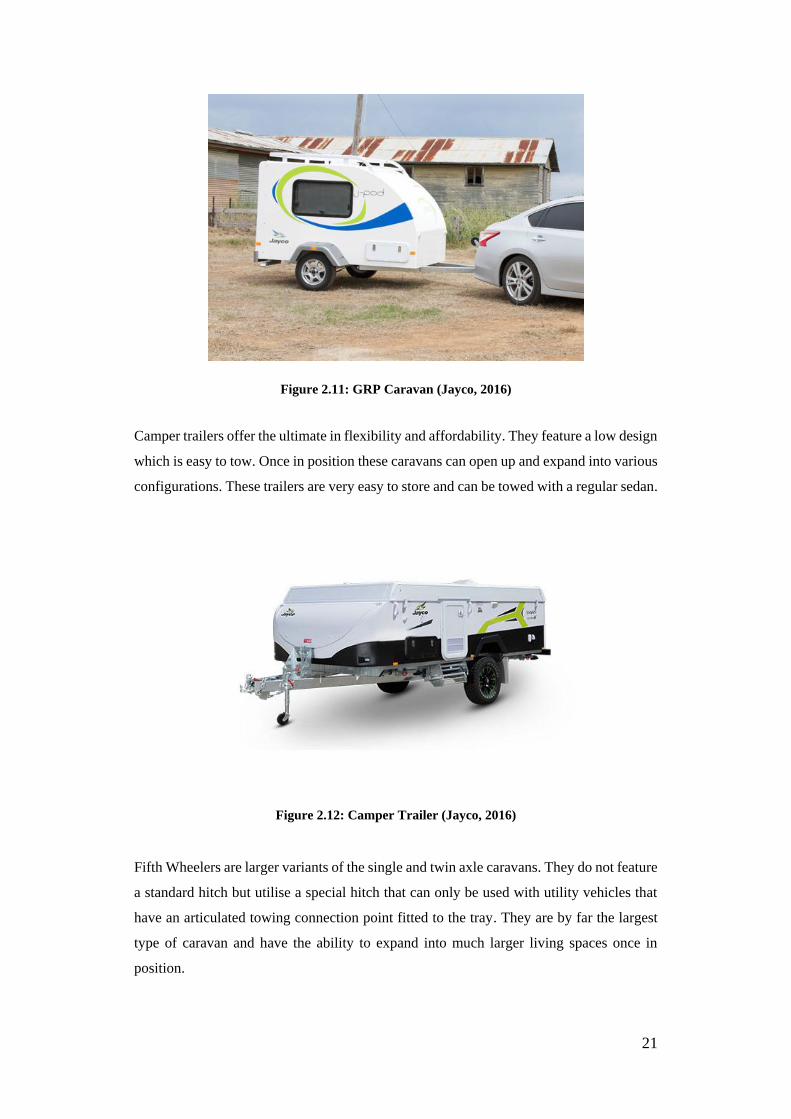
Figure 2.11: GRP Caravan (Jayco, 2016)
Camper trailers offer the ultimate in flexibility and affordability. They feature a low design
which is easy to tow. Once in position these caravans can open up and expand into various
configurations. These trailers are very easy to store and can be towed with a regular sedan.
Figure 2.12: Camper Trailer (Jayco, 2016)
Fifth Wheelers are larger variants of the single and twin axle caravans. They do not feature
a standard hitch but utilise a special hitch that can only be used with utility vehicles that
have an articulated towing connection point fitted to the tray. They are by far the largest
type of caravan and have the ability to expand into much larger living spaces once in
position.

22
Figure 2.13: Fifth Wheeler (Grey Wolf, 2016)
2.6 Computational Fluid Dynamics
Computational Fluid Dynamics (CFD) is a branch of fluid mechanics in which the Partial
Differential Equations (PDE) used to define fluid flow are approximated by algebraic
equations which are able to be solved using computer resources. Kuzmin (2012) describes
the versatility of CFD in able to solve a variety of complex problems ranging from;
meteorological phenomena, heat transfer, combustion, complex flows to human body
functions such as breathing. Its versatility is what makes it such a valuable tool to conduct
studies that previously would have taken a very long time to complete.
2.7 Application of CFD to Vehicle Aerodynamics Analysis
Computational Fluid Dynamics use over the past 30 years has increased significantly
allowing for greater flexibility and cost minimisation in many engineering projects
involving the design of both land and air vehicles. Johnson et al. (2003) has provided
insight into the evolution of design practices at the Boeing Company over three decades.
Design methods which mainly consisted of; analytic approximations, wind tunnel and
flight testing, made way to Navier Stokes equation approximations performed by powerful
computers with relative ease.
The role of wind tunnels to provide data regarding lift and drag has been an effective
method of validating design features using scale models. Johnson et al. (2003) mentions
that certain errors and complexities are introduced in the wind tunnel due to the
requirement to mount the model within the evaluation domain. This mounting method can

23
introduce interference issues with the airflow. Figure 2.14 depicts a typical wind tunnel
set up for both a land based vehicle (a) and an air vehicle (b).
(a) (b)
Figure 2.14: Wind Tunnel Test Setup (Autoevolution & NASA)
Wind tunnel testing offers the ability for designers to utilise ‘real’ conditions to test their
designs over a vast range of atmospheric parameters. Johnson et al. (2003) attributes the
success of CFD to its ability to provide an inexpensive solution to preliminary testing and
optimisation through the extrapolation of known data with the aim of providing a baseline
for future experimentation of operating parameters. It is important to note that the use of
CFD on its own is not an ideal design validation technique with most industries where
CFD techniques are commonly employed utilising a combination of CFD and physical
testing to gather the required data necessary to evaluate designs.
2.8 Application of CFD to Caravan Analysis
The majority of literature consulted regarding caravan CFD analysis is centred around
simulating the frontal drag forces. Caravan manufacturers in general have not expended
additional resources and efforts to revisit their designs which have been put into
production. Universities in collaboration with engineering companies which focus on CFD
analysis have collaborated recently to undertake studies with the aim of reducing
aerodynamic drag on existing popular designs. Glynwr University, (2011) performed a
study in collaboration with ASTUTE on a popular caravan design manufacturer by The
Fifth Wheel Company Ltd. The feasibility study aimed to study the aerodynamic flow of
air around the caravan structure and make a comparison between the effects different
towing vehicles had on the generation of drag. As a rule of thumb, aerodynamic drag forces
acting on commercial vehicles can contribute up to 60% of fuel consumption figures.

24
The study aimed to reduce aerodynamic drag by up to 20%. Through the use of CFD,
modifications were proposed and recommendations made which led to a potential decrease
in drag figures of up to 34% from the original design. This resulted in a decrease of 22.5%
of the power required to tow the caravan at speed, whilst reducing the size of the trailing
wake. Figure 2.15 depicts an example of the results obtained during this study.
Figure 2.15: CFD Simulation-Flow Modelling (Glyndwr University, 2011)
Another significant study was conducted by the Swift Group, a caravan designer based in
the United Kingdom. The study was brought about by the need to find efficiency gains
that were intended to offset the rising cost of fuel. (Swift Group, 2011) proposed that
manufacturers claimed through marketing that their caravans were aerodynamic but this
was mainly based on subjective data using rudimentary methods such as towing trials.
Swift Group contracted a CFD specialist to undertake a 3D scan of their caravans and
utilise these models to simulate the flow of air around the caravan. This CFD study was
complemented by concurrently running wind tunnel tests on their caravans. As a result
Swift Group was able to implement a weight reduction program and coupled with further
streamlining of their caravan designs were able to significantly reduce the running cost
involved with towing their products. Figure 2.16 depicts a near wall velocity study
conducted using CFD.

25
Figure 2.16: Near Wall Velocity CFD Study (Swift Group, 2013)
Although there is significant evidence available to confirm the benefit of conducting a
CFD study on caravan from a frontal profile perspective, the effect of cross wind influence
on the geometry is not as widely published as is found with other transportation methods
such as trucks and trains.
2.9 CFD Pre-Processing
An essential function of performing a CFD analysis involves the preparation of the model
geometry and the mesh in order to configure the solver to be able to produce the best
results possible with as little effort as possible. At a minimum the process can be defined
by (ANSYS Release 14.5 Documentation, 2012) as;
1. Create the geometry
2. Simplify the geometry
3. Define the mesh resolution required
4. Define the mesh type required
5. Assess computing resources available
26
2.9.1 Development of Geometry
An important consideration when configuring the CFD software package to commence
solving a problem is to ensure the geometry in which the airflow will be simulated through
is optimised for the particular model being tested. (Keating, 2010) states that by following
some pre-processing guidelines, reliable results can be obtained time after time. In order
to set up the simulation environment optimally the following questions should be asked;
What do you want to do and gain from the CFD analysis?
What are the driving parameters?
What zones need to be separate for constraints or post processing?
What fluids zones will be replaced?
What level of geometric representation is needed?
It is also emphasised that small changes can have large effects.
2.9.2 Mesh Generation
Mesh quality is an important consideration when undertaking a CFD analysis. Keating,
(2010) agrees with other literature sources in emphasising that the quality of the mesh goes
a long way to providing accurate and reliable results. Generating a mesh often requires
significant time and computing resources depending on the complexity and geometric
configuration of the mesh required. It is however important to note that at this point the
investment made in generating a good mesh pays greater dividends when it comes to
generating a solution.
Bakker, (2002) states that hexahedral meshes offer the best solution, with the accuracy of
the solution becoming even greater when the mesh grid lines are aligned with the flow.
Quality of a mesh is defined by the following three features; Skewness, Smoothness and
Aspect Ratio.
Skewness in the cell geometry should be avoided. Increases in cell size should be
incrementally smooth and finally an aspect ratio for mesh cells of 1 should be strived for
27
as featured in squares and equilateral triangles. Keeping the mesh quality high will ensure
that solutions are as accurate as possible.
2.9.3 Establishment of Boundary Conditions & Turbulence Models
In order to establish the context of the simulation and define the domain in which the solver
will calculate for, it is vital that the correct boundary conditions be established and that the
correct model be selected depending on the type of problem. There is significant amounts
of literature which highlight the pros and cons of the most common turbulent flow models
employed by the major CFD software packages. These models aim to represent the Navier-
Stokes equations as accurately as possible through the setup of a simulated wind tunnel,
however accuracy is limited by the amount of processing resources and the discretisation
size of the domain.
Frei (2013) conducted a comparison exercise to highlight the advantages and
disadvantages of the most commonly used turbulent models used in CFD practices. Table
2 presents the findings of this review.

28
Table 2: Turbulence Model Comparison (Frei, 2013)
Model Advantages Disadvantages Applicability k-epsilon (k-ε) Good Convergence Rate
Requires less computing
resources
Reasonable prediction of
different flow types
Utilises wall functions
Applicable only to
fully turbulent
flows
Difficulty in
predicting the
following;
Swirling or rotating
flow
Adverse pressure
gradients
Airflow simulation
around bluff bodies
Industrial
applications
Simulation of
Complex geometries
Axisymmetric jet
flow
k-omega (k-ω) Ability to simulate for flows
that feature;
Internal Flows
Separated flows
Jet airflow
Sensitive to initial
guess of solution.
Difficulties in
reaching
convergence
Requires pre-
processing through
k-epsilon model to
aid in accuracy
Simulation of Internal
flows.
Used in modelling
fluid flow through
pipes and ducts.
Low Reynolds
k-epsilon
Higher Accuracy in
modelling lift and drag
forces.
Requires higher
computing
resources
Simulation of Lift
and Drag forces
around bodies.
Heat flux simulation
problems
Shear Stress
Transport
(SST)
Accurate for solving flow
near walls.
Utilises k-epsilon modelling
technique for free stream
flow and k-omega model in
the wall region.
Somewhat slow to
reach convergence. Effective in handling
similar problems as
detailed in k-epsilon
and k-omega sections.
The two equation models (k-ε & k-ω) feature the greatest flexibility for most applications.
Frei, (2013) promotes the k-epsilon model as the most versatile of the turbulent models as
it combines the two variables k; turbulent kinetic energy, with ε ; the rate of kinetic energy
dissipation, in order to provide somewhat quick results with known inaccuracies in dealing
with laminar flow. The true effectiveness of the turbulent models are centred around the
ability of the model to capture what is occurring in the boundary layer between the laminar
layer at the wall of the surface and the turbulent layer above. Figure 2.17 depicts the
boundary profile of the airflow. By utilising wall functions in models such as k-epsilon in
order to simulate flow in the buffer region, the model can utilise approximations in order

29
to reduce the computational requirements and therefore leading to a more rapid and less
resource intensive solution. On the other hand, for increased accuracy at the boundary
layer the k-omega model provides a greater degree of accuracy, due to its computational
method without the use of wall functions. It is however noted from Table 2 that the
resources required are much higher and convergence is also somewhat difficult to achieve.
The Shear Stress Transport (SST) method provides a more accurate solution when
considering the boundary layer. Karthik (2011) defines the SST model as an eddy-
viscosity model which combines the previously discussed two-equation models in
combination to model the buffer layer with greater accuracy. The k-ε provides a model for
the region outside the boundary layer, whilst the k-ω models the region inside the boundary
layer.
When assessing the requirement to use a particular model for a study, two main
considerations need to be factored into account. Frei (2013) highlights the requirement to
utilise a problem mesh which is as simple as it can be in order to obtain the desired level
of accuracy. Secondly, the turbulence model selected should provide results which strike
a balance between computational resources, processing time available and accuracy of the
solution.
Figure 2.17: Flow regimes at the Wall Interface (Frei, 2013)

30
2.10 CFD Solver
The simulation process performed by CFD software packages such as ANSYS generally
utilise a two-step approach in order to compute a solution (ANSYS Fluent Documentation,
2006). These steps can be defined as Numerical Model Setup and
Computation/Monitoring of solution. Together they form the core function referred to as
the Solver Execution.
The numerical model setup process generally comprises the following elements according
to Ahmadi & Nazridoust (n.d);
1. Selection of an appropriate physical model for the simulation: combustion, turbulence
etc.
2. Define the material properties; fluid, solid or mixture.
3. Prescribe operating conditions; temperature, pressure, velocity etc.
4. Prescribe the boundary conditions
5. Produce Initial Solution
6. Set up Solver Controls
7. Monitor Convergence
The computation and monitoring phase deals primarily with the discretization of the
conservation equations or Navier Stokes equations which are solved iteratively until
convergence is reached. Convergence is deemed to be obtained when the difference in
solution data from one iteration to another is negligible verifying the numerical accuracy
of the solution. Convergence can therefore be used to validate the accuracy of a solution
as it changes over time.
Convergence is monitored through the use of ‘residuals’. Kuron (2015) describes residuals
as one of the most fundamental measures of iterative convergence, as it provides a direct
numerical representation of the error involved in the solution of the system of equations.
Figure 2.18 depicts an example of a common residual plot with the variable value (Y-Axis)
plotted against an Accumulated Time Step (X-Axis).

31
Figure 2.18: Residual Monitors
It is important to note that because a residual represents the absolute error between two
iterations of a solution it is therefore ideal that the error be reduced to a value as close to
zero as possible. Throughout the majority of literature reviewed convergence can be
deemed to be roughly achieved when the Root Mean Squared (RMS) residual levels are
less than a value of 1×10⁻⁴ and residual levels of 1×10⁻⁵ are deemed to be well converged
(Kuron, 2015).
Convergence with regard to CFD applications can also be identified through the
monitoring of points of interest. Gelman et al (2003) describes the error in defining
convergence if a simulation is not left to run for an extended period of time. By monitoring
individual points in a variable solution over a defined number of iterations, convergence
is said to be reached when fluctuations decrease to a small amount in the order of 1×10⁻⁴
- 1×10⁻⁶. This can usually be represented by a relatively flat ‘tail’ in the plot as depicted
in Figure 2.19.
Figure 2.19: Monitor of Point of Interest (Thoms, 2007)

32
2.11 CFD Post Processing
Once the solver has performed the simulation and has generated the required data sets, the
data must be processed through specific software, namely ANSYS CFD Post, which
provides a post processing capability to ANSYS Fluent and CFX. This process is required
in order to manipulate the data and generate the required numerical and visual
representations that can be tailored to the output parameters required. These
representations can take the form of streamline plots, pressure gradients and velocity
scalars/vectors as well as reports which can depict histograms of data. An important
consideration in performing effective post processing functions is to gain a good
understanding of what data is required in order to draw the necessary conclusions and how
that data can be manipulated to produce effective graphical representations of information
to support both quantitative and qualitative discussions of results.
2.12 Force Coefficient Calculation
Malviya, Gundala & Mishra (2009) undertook a study to determine an effective way to
calculate the coefficient of drag, lift and side force for ground based vehicles subject to a
crosswind.
The three main equations used in the calculation of these forces are;
𝐹𝐷 =𝜌𝐶𝐷𝐴𝑣2
2
𝐹𝐿 =𝜌𝐶𝐿𝐴𝑣2
2
𝐹𝑠 =𝜌𝐶𝑠𝐴𝑣2
2
Where 𝐶𝐷, 𝐶𝐿 and 𝐶𝑆 represent the coefficients of Drag, Lift and Side Force respectively.
A represents the characteristic frontal area of the vehicle and can be calculated for different
areas presented to the flow when the vehicle is under yaw. The trigonometric relationship
for the characteristic area A is calculated using the equation;
𝐴 = (𝑙 × 𝑠𝑖𝑛𝛼 + 𝑤 × 𝑐𝑜𝑠𝛼)ℎ

33
Where l = length of vehicle,
w = width of vehicle, and
h = height of vehicle
In order to calculate the characteristic area of the vehicle combination it is common
practice to represent the vehicle as rectangular boxes multiplying the area by a factor of
0.85 for cars and a factor of 1 for truck/trailer combinations. It was decided that for this
scenario that a value of 0.95 would be appropriate given the rectangular nature of the
vehicles in question.
2.13 Literature Review Summary
It is evident throughout the literature reviewed that designers, manufacturers and
researchers have conscientiously applied themselves to the purpose of enhancing the
aerodynamic efficiency of vehicles in order to reduce operating costs and benefit from
increases in speed and handling.
From the literature review it is also evident that there has not been any specific attempt to
address the effect that crosswind flow has on a car and caravan combination. It is however
noted that the studies conducted into truck & trailer combinations and high speed trains
under crosswind raise some interesting points, these observations and suggestions for
modifications can be carried across to the caravan.
The literature concerning the use of Computational Fluid Dynamics by computer
simulation programs such as ANSYS has been reviewed with valuable insight gained into
how the approach can be useful in order to simulate how a system will perform in ‘real
world’ conditions. The literature provided valuable guidance in how to set up the problem,
run the simulation and then interpret the results.
34
CHAPTER 3 – RESEARCH METHODOLOGY
3.1 Overview
This chapter will outline the methodology in carrying out the parametric study on the tow
vehicle/caravan combination. The process followed in establishing the geometry profiles
of the model which will be used in the CFD study will be discussed along with the CFD
parameters which will be evaluated in order to provide the best setup for the initial study
and provide a suitable platform for the post modification analysis phase. As this project is
predominantly concerned with evaluating the effect that the proposed modifications to the
caravan’s design has on the overall drag force, the tow vehicle model once established will
not be altered in any way.
3.2 Vehicle Selection
As mentioned in section 2.4, the study will utilize the Land Rover Discovery 4 as the tow
vehicle. The vehicle was selected due to the availability of data captured through previous
studies which would allow for a general comparison between current and previous results.
This would also assist in validating the approach used which would be difficult if an
arbitrary geometry were utilized instead to represent the tow vehicle.
The geometry and vehicle characteristics have been modelled based on the specifications
provided by Land Rover in the Discovery 4 product brochure as detailed in Appendix D.
3.3 Modelling Technique
The initial approach used to generate the model of the tow vehicle involved utilizing the
3D modelling software package PTC Creo Parametric 3.0 to produce the model that would
be imported into ANSYS. The reasoning behind the selection of this modelling method
was partly due to having familiarity with the program whilst also being able to produce
complex geometry features with relative ease. Figure 3.1 depicts the first vehicle model as
modelled in Creo Parametric. This model consisted of a body that represented the profile
of the LandRover Discovery 4 whilst featuring simplified wheel geometry.

35
Figure 3.1: Original Land Rover Model (Creo Parametric)
The model was created as a part with a large amount of features which allowed for a close
representation of the actual vehicle. The model would be exported to an IGES/STEP file
format allowing it to be imported into ANSYS easily. It was noted however that due to the
simplified model features predominantly involving the wheels and wheel arches a
significant reduction in drag would be obtained which would not truly reflect the actual
vehicle. It was noted throughout the research conducted as part of the literature review that
wheel arches and external protrusions such as mirrors contribute to the frontal drag profile
of the vehicle, therefore it was decided to include these features in the final model.
Figure 3.2 depicts the final geometry which included most of the features that would
accurately depict the true configuration of the actual vehicle.

36
Figure 3.2: Simplified Land Rover Model (Creo Parametric)
The model produced conformed to the Land Rover dimension specifications and allowed
for the inclusion of wheel arches, complete wheel and tyre assemblies and side mirrors. It
was also noted that this modelling option provided the simplest method of carrying out
modifications to a geometry as it is all handled within the same program therefore negating
the requirement to learn a new modelling language and conventions It was anticipated that
based on the number of ANSYS simulations required and reconfiguration tasks to be
conducted, that a portion of time would need to be allocated to exporting and importing
geometry which needed to be factored for in the project timelines. It was noted however
that a benefit of modelling with an external package allowed the user to perform ANSYS
simulation in the background, whilst allowing for modelling work to continue in CREO.
3.4 Vehicle Geometry
The first step in developing the model of the tow vehicle within CREO was to create a
rectangular boundary oriented with the x-y plane that would provide the general dimension
outline of the vehicle. This would allow for the vehicle to be modelled in proportion to
this boundary. The defining dimensions in this first step included; ride height, vehicle
length, vehicle height and wheelbase.
The outline of the vehicle was sketched within this boundary and dimensioned
accordingly. Once the outline of the vehicle was deemed to be suitable the sketch was then

37
extruded in the z dimension to a width representing the width of the vehicle minus any
extruded features.
Chamfers and blends were then added to the extruded solid to provide a closer
representation to the actual vehicle. Wheel arches were added by sketching two circles to
the required size and then subsequently cutting material away to a depth that would
accommodate the wheels. Once the wheel arches were in place the wheels were added
sketched and extruded to the specifications provided by Land Rover.
Once all features were in place an additional reference plane was created and translated to
a distance from the sketch face that represented the mid plane of the vehicle. Subsequently
all features were mirrored about this plane. Side mirrors were modelled and mirrored about
the mid plane completing the vehicle geometry.
Figure 3.3 depicts the model imported into ANSYS Workbench
Figure 3.3: Model imported into ANSYS.
An important modelling characteristic to note was that the model was created in its entirety
and not represented by half the geometry as was represented in the study conducted by
Briskey, 2013. Although it is expected that modelling half the geometry would be
satisfactory for a headwind analysis the requirements for undertaking a crosswind analysis

38
required the entire geometry be modelled to ensure all features of the vehicle are factored
into the analysis.
3.5 Fluid Domain
With the geometry of the vehicle established, the fluid body moving around the vehicle
required consideration. To simulate a ‘wind tunnel’ like set up an enclosure around the
vehicle was generated. The enclosure was created using the enclosure tool and was
subsequently subtracted from the vehicle geometry by using the Boolean tool. The
enclosure was set up to allow for enough room forward of the vehicle to allow the airflow
to stabilise and with sufficient volume aft of the vehicle to allow for the airflow to re-join
and stabilise. The initial enclosure was non-uniform in nature and is represented in Figure
3.4. Further details regarding the experimentation with enclosure size is discussed in
section 3.10
Figure 3.4: Non Uniform Enclosure

39
3.6 3D Model Validation
In order to assess the validity of the model prior to progressing with the study a set of
criteria was established to allow for the model to be considered reasonably similar to the
actual vehicle.
The criteria to assess the model against was as follows;
1. Geometric Similarity
2. Coefficient of Drag (Cd)
Due to the technique of modelling the vehicle utilising a certain element of approximation
regarding dimensioning, the emphasis was placed on ensuring that the frontal area of the
vehicle closely matched the actual vehicle. This was important due to the requirement of
using area as a variable in the coefficient of drag equation. Due to the rectangular frontal
profile of the 2016 Land Rover Discovery 4 the frontal area was simple to calculate with
a high degree of certainty by multiplying vehicle height by the width.
2
1.92 2.20
4.224
frontal
frontal
frontal
A Height Width
A m m
A m
Once a frontal area value was established a simulation was conducted in CFX with a
monitor point set up to identify the drag force in the x-direction on the vehicle body. The
velocity of the vehicle for this baseline calculation was set at 80 km/hr (22.22 m/s). Based
on the information captured through the literature report, the Land Rover Discovery 4 had
a Coefficient of Drag of 0.4. Figure 3.5 depicts the force in the x direction on the surface
of the vehicle.

40
Figure 3.5: Drag Force in X and Z directions on Vehicle
Utilising this value at convergence and inputting into the coefficient of drag equation a
baseline Cd was obtained that would provide an indication on how valid the model was in
comparison to the actual vehicle. From section 2.4.1 it can be seen that the Coefficient of
Drag once calculated was initially determined to be;
2
23 2
2
2 568
1.22 / 22.22 / 4.224
0.45
D
d
frontal
d
d
F
v A
N
kg m m s m
C
C
C
As the Cd figure is approximately 12% greater than the stipulated value provided by Land
Rover, it is therefore a valid model to continue the study with. Due to the simplification of

41
key features an increased coefficient of drag was to be expected. Further alterations to the
design of the vehicle were seen to not provide any viable improvement in Cd figure when
compared to the effort and time required to alter the model.
3.7 Mesh Setup
Once the initial geometry of the vehicle was created the simulation moved into the meshing
phase. It was vital that this process was carried out diligently as the accuracy of any results
would be attributed primarily to the quality of the mesh. As the meshing process used is
generally tailored towards a particular model or desired outcome it was important to
establish a baseline mesh which could be altered in various ways to refine the solution.
Once this mesh was deemed appropriate it could be used to undertake a Grid Independence
Study were these meshing parameters could be experimented with to validate the solution
and more importantly the setup.
As the ANSYS analysis system to be used for this study was CFX, it was important to
select the correct Physics and Solver preference from the meshing defaults to suit the study
type. The default setting was set as;
Physics Preference: CFD
Solver Preference: CFX
3.8 Global Mesh Sizing Control
Following on from establishing the physics based settings of the mesh, the global mesh
sizing controls. The sizing features that would be considered for meshing are; Relevance
and Relevance Center, Advanced Size Functions (ASF), Smoothing, Transition & Span
Angle Center. For the initial setup it was decided to evaluate the relevance and advanced
sizing functions only to allow for a baseline mesh that could be refined even further during
the Grid Independence Study as detailed in section 3.9.

42
3.8.1 Relevance and Relevance Center
The relevance and relevance center are important meshing controls as they allow for the
global refinement of the mesh which results in a coarsening of the mesh. By utilising these
settings the fineness of the mesh can be easily altered through the use of a sliding scale for
relevance and through the selecting between three available settings in Relevance Center.
The relevance sliding scale allows for the adjustment of the mesh between a range of -100
to 100 with 0 being the defaulted value. Moving in a negative direction results in a coarser
mesh to begin with which allows for a quicker solution time however the accuracy of the
solution is diminished. Moving in a positive direction results in the application of a finer
mesh which will provide more accurate results albeit with longer solving times. As the
defaulted value is 0 and there are 200 increments to solve for it was decided that any
refinement to meshing would be carried out using the Relevance Center thus saving time.
The relevance center simplified the meshing sizing selection process by offering only 3
variables; Coarse, Medium and Fine. For the initial setup of the vehicle it was decided to
commence with a medium mesh allowing for further refinements to be carried out in the
Grid Independence Study.
3.8.2 Advanced Size Function
The advanced sizing functions allow for the control of meshing growth in critical locations
such as curvatures or surfaces. Five options are available for selection; Off, Proximity and
Curvature, Curvature, Proximity and Fixed. Off is selected by default. The curvature
component of the ASF allows for the mesh to be formed along the edge of a boundary and
face with relation to the Curvature Normal Angle hence creating a finer mesh around
curves. The proximity feature of allows for the distribution of a defined number of
elements into area such as gaps. Figure 3.6 depicts an example geometry with ASF set of
Off in comparison to Proximity and Curvature.

43
Figure 3.6: ASF Meshing Comparison (Leap Australia, 2011)
For this study the combination of both curvature and proximity would be used as it
provided a good balance between mesh detailing at critical locations. Figure 3.7 depicts
the mesh around the wheel when the ASF is set to Proximity and Curvature.
Figure 3-Proximity and Curvature ASF mesh detail
3.8.3 Initial Mesh
The initial mesh setup featured a medium mesh which allowed for a faster solution time
in order to validate the vehicle model initially. With the ASF set On: Proximity and
Curvature a higher level of detail was maintained at the edge boundaries of the vehicle

44
with the mesh becoming coarser as it moved away from the edge boundaries. The fluid
domain meshing was deemed acceptable at this level of detail as the priority at this stage
was ensuring the vehicle boundaries were detailed enough to get a good starting point,
prior to refining. At this point it must be noted that the solution time was a large
contributing factor to establishing what initial mesh would give an adequate result. Figure
3.8 depicts the initial mesh of the tow vehicle within the enclosure. Figure 3.9 provides a
detail view of the initial vehicle mesh.
Figure 3.8: Isometric View of Meshed Domain

45
Figure 3.9: Detail View of Initial Vehicle Mesh
3.9 Grid Independence Study
A Grid Independence Study was seen as an important process to ensure that the initial
mesh characteristics were suitable prior to applying them to other elements of the study
namely the caravan. During the initial run to calculate the Cd of the vehicle, the monitor
points for Momentum and Mass being RMS P-Mass, RMS U-mom, RMS V-mom and
RMS W-mom in addition to the Turbulence Monitor Points being RMS K-TurbKE and
RMS O-TurbFreq, were monitored for convergence based on residual value difference
established through CFD literature in the order of 10-4.
When making changes to the mesh detail it is vital that the solver be run to ensure that
meshing detail does not affect the validity of the solutions. Once the solution is established
with values that are not significantly different to each other it can be decided on a final
mesh detail. For the purposes of this mesh independence study the solver was set to 250
iterations. Any solution not achieved by this time step was deemed not converged and as
a result the computation time for this study reduced.
The following figures in Table 3 were obtained regarding the meshing detail through the
selection of various mesh sizing features in the mesh relevance centre.

46
Table 3: Relevance
Relevance
Centre
Elements Nodes Convergence
Iterations
Force_x (N)
Land Rover Model
Coarse 748463 525438 76 568
Medium 1083489 757284 120 569.9
Fine 1309508 911546 86 568
Mesh smoothing aims to improve the quality of the mesh by arranging the location of mesh
nodes in relation to surrounding nodes. ANSYS offers three levels of smoothing, these
are; Low, Medium and High. As a general rule CFD studies are conducted with a
smoothing setting of medium. Table 3 details the results obtained through variation of
smoothing settings based on the default CFX meshing settings.
Table 4: Smoothing
Smoothing Elements Nodes Convergence
Iterations
Force_x (N)
Land Rover Model
Low 1297265 902593 113 568.1
Medium 1309508 911546 120 569.9
High 1307431 909915 84 568.6
Transition sizing refers to the rate at which mesh elements grow. There are two control
levels that define mesh transition, they are; Slow and Fast. Slow provides a more gradual
size transition whereas Fast produces a more rapid and abrupt transition in the mesh. Table
5 details the result variation between both control levels
Table 5: Transition Sizing
Transition Elements Nodes Convergence
Iterations
Force_x (N)
Land Rover Model
Slow 1656797 310443 100 566.03
Fast 574590 120596 99 647.46
Span Angle Centre allows for the control of the mesh refinement based on curvature along
the edges. The mesh will elements will subdivide in order to span the distance between
edge angles. The three settings available are; Coarse (91º to 60º), Medium (75º to 24º) and
Fine (36º to 12º). Table 6 lists the figures obtained.

47
Table 6: Span Angle Centre
Span Angle
Centre
Elements Nodes Convergence
Iterations
Force_x (N)
Land Rover Model
Coarse 916072 176032 82 567.4
Medium 988928 189182 136 564.7
Fine 1176190 220867 145 528.6
3.10 Enclosure Dimensioning
An important consideration when establishing the fluid domain around the target vehicle
is the enclosure sizing. Due to the configuration of the model being studied the enclosure
was initially created with Design Modeller to be a non-uniform bounding box. The
dimensions of the original enclosures for the tow vehicle were set as follows;
Table 7: Enclosure Dimensioning
Coordinate Configuration 1 (m) Configuration 2 (m)
+X 25 20
-X 15 10
+Y 5 5
-Y 0.001 0.001
+Z 5 10
-Z 5 10
Force x (N) 568 524.2
The enclosure (Configuration 1) was deemed adequate for the study involving the tow
vehicle in isolation. When the caravan assembly was imported into the domain, the
enclosure automatically adjusted to maintain the same boundary distances.
3.11 Final Mesh Detail
After conducting the grid independence study the following settings were selected for use
for the rest of the analysis. The setting selection was based on two competing factors. The
first of these was accuracy of the result at convergence. This was compared against the
computing resources required as evident in the solution times. In order to proceed with a

48
setup that would produce the best results given the circumstances an assessment of results
was conducted with the final mesh settings in the following table;
Table 8: Mesh Options
Mesh Option Selection Defaults:
Physics Preference
Solver Preference
Relevance
CFD
CFX
0 (default)
Sizing:
Use advanced size function
Relevance Centre
Initial Size Seed
Smoothing
Transition
On: Proximity and Curvature
Medium
Active Assembly
Medium
Slow
Inflation:
Use automatic Inflation
Inflation Option
Transition Ratio
Maximum layers
Growth Rate
None
Smooth Transition
0.77
5
1.2
Statistics:
Nodes
Elements
Mesh Metric
None
This mesh was applied to the caravan and tow vehicle configuration with the following
mesh dimensions
Nodes: 119876, Elements: 575961
3.12 CFX Simulation Setup
Once a suitable mesh was established through the grid independence study it followed that
the tow vehicle and caravan model were imported into the solver and the mesh applied to
both entities. The setup of the CFX simulation is detailed in the following section.
3.12.1 Fluid Model Configuration
The fluid properties for use in this analysis are the first critical parameters to set up. As a
variety of different atmospheric properties would exist in reality which are linked to
various geographic and physical locations it is vital that the CFD study be conducted with
fluid properties that would represent an accepted standard ensuring that all results could

49
be benchmarked against these conditions. The default properties for air were adopted in
this case. They are as follows;
Air with temperature of 25ºC
Pressure of 1 atm
Air Density – 1.22 kg/m3
The other consideration involved selecting the most appropriate fluid model. From the
literature review conducted it was decided that the Shear Stress Transport (SST) model
was the most appropriate model to use in this analysis as it offered the best accuracy for
boundary layer flow.
Transient flow was not considered therefore the solution was set up as a Steady State
analysis.
3.12.2 Domain Initialisation
Following the selection of the fluid properties it was necessary to set the initial conditions
required for subsequent tests. As the orientation of the model within the domain was set
to change to factor in for wind direction, it was necessary that each run was conducted
with the correct initial values for the various components of wind.
Initially the straight on test for the purpose of selecting the appropriate mesh was
conducted using the wind speed of 80 km/h in the Cartesian direction U which applies to
the x axis. The turbulence option was left at the default setting of Medium which set the
value (Intensity = 5%).
3.12.3 Boundary Setup
The following tables list the boundary conditions for the analysis in CFX.
Table 9: Inlet Boundary Details
Boundary Feature Properties
Inlet:
Type
Flow Regime
Mass & Momentum Option
Normal Speed
Turbulence
Inlet
Subsonic
Normal Speed
80 km/h
Medium (Intensity = 5%)

50
Figure 3.10: Inlet Boundary CFX
Table 10: Outlet Boundary Details
Boundary Feature Properties
Outlet:
Type
Flow Regime
Mass & Momentum Option
Relative Pressure
Pres Profile Blend
Outlet
Subsonic
Static Pressure
0 Pa
0.05
Figure 3.11: Outlet Boundary CFX

51
Table 11: Opening Boundary Details
Boundary Feature Properties
Opening:
Type
Flow Regime
Mass & Momentum Option
Relative Pressure
Flow Direction
Turbulence
Opening
Subsonic
Opening Pres and Dim
0 Pa
Normal to Boundary Condition
Medium (Intensity = 5%)
Figure 3.12: Opening Boundary CFX
Table 12: Road Boundary Details
Boundary Feature Properties
Road:
Type
Mass & Momentum
Wall Roughness
Wall
No Slip Wall
Smooth Wall

52
Figure 3.13: Road Boundary CFX
Figure 3.14: Complete Boundary Setup CFX

53
3.12.4 Monitor Points
User monitor points for frontal drag in x direction set up in CFX Output control as
Expression force_x()@Default Domain Default. An additional monitor point used to
monitor the drag in the z direction is used in the analysis of crosswind flow. The expression
used in this case is force_z()@Default Domain Default. Additional Monitor Point
expressions were able to be set to automatically capture key aerodynamic parameters such
as coefficients of both lift and drag. It was decided that these additional expressions were
not required as the force figures could be used to manually calculate the subsequent
Coefficient of Drag values with little effort.
3.12.5 Solver Control Setup
The Solver Control Setup settings with CFX-Pre allow for setup of key simulation
parameters
Table 13: Solver Control Details
Solver Control Basic Settings Settings
Advection Scheme Option
Turbulence Numerics Option
Minimum Iterations
Maximum Iterations
Timescale Control
Length Scale Option
Timescale Factor
Residual Type
Residual Target
High Resolution
First Order
1
250
Auto Timescale
Conservative
2
RMS
1.E-4
3.12.6 Solution Component Setup
In order to maximise the processing power of the computer hardware used for the CFD
Analysis some specific settings can be chosen that will utilise the maximum potential of
the computing system. The processor used for this study is the Athlon X2 245 with a clock
speed of 2.9 GHz. The processor has dual core capability allowing it to simultaneously
utilise both cores to perform CFD computations as well as manage computer background
tasks.
When defining the run, the selection Platform MPI Local Parallel was made. This utilised
2 partitions to perform the run.

54
Figure 3.15: Solver Run Settings
3.13 Caravan Selection
Without the provision of a caravan model to utilise in this study by way of a project
sponsor, it was necessary to select a caravan design and produce a model for use in the
study. After a review of literature the design to be analysed was based around a
combination of features as displayed by the following three caravan models. They are;
Jayco Starcraft
Trakmaster Simpson
Majestic Knight
The final caravan model as produced in CREO provided an average representation of all
three caravan models researched.

55
Figure 3.16: Jayco Starcraft (Jayco, 2016)
Figure 3.17: Trackmaster Simpson (Trackmaster, 2016)

56
Figure 3.18: Majestic Knight (Majestic Caravans, 2016)
3.13.1 Caravan Geometry
The dimensioning for the caravan was based off the Jayco Starcraft with a length of 5.33
m, width of 2.3 m and a height of 2.89 m. The caravan features a standard draw bar length
of 1.8m and travels upon on a twin axle wheeled arrangement.
The caravan was modelled by starting with a rectangle to provide the boundary for the
external geometry. From here the outline was drawn and then extruded to the required
width. The wheel arched were drawn and then extruded using the remove material
function. The wheels were subsequently modelled and finally the drawbar ‘A-Frame’ was
modelled. When all the major components were modelled some chamfers and rounds were
added to the frontal profile of the caravan. The model was added to the LandRover model
and saved as an assembly file. From here the assembly was exported to IGES format for
use within ANSYS. Figure 3.19 depicts both the front and side profile of the modelled
caravan.

57
Figure 3.19: Final Caravan Model
3.13.2 Caravan Meshing
Given the similarity in some of the caravan geometry to that of the tow vehicle it was
decided to commence the study with the same mesh as was used in the tow vehicle. This
also ensured that the features of the caravan such as wheels and wheel arches retained a
higher quality mesh without featuring a very large number of elements which would
subsequently extend the computation time. Figure 3.20 depicts the final mesh used for the
caravan assembly.

58
Figure 4: Car & Caravan Model Mesh
The model was rotated within the enclosure to reflect the wind direction and then the
simulations were carried out. It was noted that with simulating wind impingement angles
of less than 30º the solutions took very long to converge and in some cases did not
converge at all. The transition sizing was changed to fast for investigation and some
observations regarding convergence that altered the mesh for the combined assembly.
Firstly, the solution converged with very minor imbalances in the RMS residuals.
Secondly convergence occurred in approximately 50% of the iterations required by the
slower transition mesh. Finally when comparing the results between both converged
solutions the difference in monitor point results was generally in the vicinity of being under
1% different. It was therefore decided that in the interest of keeping computation time to
a minimum given time and physical resources that this error could be considered
reasonable and allow the pre-optimization and parametric study to continue.

59
3.14 Caravan CFX Simulation
From force monitor point image – Force measured as 1436 N
The Coefficient of Drag for the combined test model was calculated by;
Figure 3.21: Car Caravan Boundary Set Up at Zero Yaw
2
23 2
2
2 1436
1.22 / 22.22 / 6.65
0.72
D
d
frontal
d
d
F
v A
N
kg m m s m
C
C
C

60
Figure 3.22: Force Monitors Graph for Baseline Caravan
Figure 3.23: Residuals-At convergence (Caravan Set Up)

61
3.15 Summary of Results
LandRover Discovery 4 model produced 568 N of drag force in x direction. Fuel
consumption figure from OEM specifications of 8.8 L/100km (Combined). For the
purposes of this study the increase in drag force produced by the caravan will be divided
by the Landrover force and then used to extrapolate fuel economy figures.
Given a force of 1436 N produced in the tow vehicle caravan combination, then
preliminary fuel consumption for the vehicle when towing the baseline configuration
caravan will be;
2.52 8.8
= 22.2 L/100 Km

62
CHAPTER 4 – PRE-OPTIMIZATION STUDY
A study was conducted on the car and caravan combination prior to modification in order
to gather some initial data. This data would be compared against post modification results
to ascertain whether any advantages could be gained from implementing the modification
to the baseline configuration.
The first part of this study involves verifying the flow patterns that are present around the
tow vehicle and caravan combination in various cross wind configurations and the forces
at play on the vehicles in a static set up. The configurations for the tests were as follows;
Wind Speed varied of values 50, 80 and 100 km/h
Relative Wind Vector Angles of 0,15,30,45 & 60 degrees.
The major quantitative areas of interest that can be used to make an informed qualitative
assessment of the flow patterns and aerodynamics of the caravan include the following;
Flow Velocity
Forces in X, Y and Z coordinates
Turbulent Kinetic Energy
Pressure Gradients
The car and caravan combination was simulated under the flow conditions detailed above
and the following initial results were obtained. These results would be used for comparison
during the parametric study detailed in Chapter 5.
4.1 Wind Loading Forces
By setting up monitor points to record the forces experienced on the models surfaces in
three dimensions it is possible to make some observations regarding the effect wind speed
and wind angle have on the car and caravan. The following graphs represent the forces in
their respective dimensions. The data for these graphs is located in Appendix E.

63
4.1.1 Drag Force in X Direction
Figure 4.1: Force in X Direction for Baseline Caravan
It can be observed that as the velocity of the wind flow increases the forces produced
increase exponentially, this can be attributed to the kinetic energy relationship with the
force produce at double the velocity being 4 times as great.
As the model is rotated within the flow the forces in the x direction increase. It is noted
that the rotation angles between 15 and 45 degrees show the greatest increase in force
produced. This can be attributed to the side of the model coming into play presenting itself
to the airflow
0
2000
4000
6000
8000
10000
12000
0 15 30 45 60
Forc
e (N
)
Wind Angle
Force x for Baseline Caravan
Force x at 50 km/h
Force x at 80 km/h
Force x at 100 km/h

64
4.1.2 Lift Force in Y Direction
Figure 4.2: Force in Y Direction for Baseline Caravan
As with the force in the x direction it can be also seen that as the velocity increases the
force is seen to increase as is expected from the kinetic energy equation relationship. As
the caravan is rotated to orient itself 15° into the flow it can be seen that the force decreases
slightly until the caravan is rotated to the 30° angle where it increases steadily.
The increase in lift forces can be attributed to the exposure of leading edges to the flow as
the caravan rotates through to 60° rotation. These leading edges are generally rounded and
increase the velocity of the fluid flowing over them as is seen with the front roof section
of the caravan.
4.1.3 Side Force in Z Direction
As the wind angle is altered from 0° through to 30° it can be seen from the data collected
that the force increases rapidly due to a greater surface area being presented to the flow.
As the angle increases past 30° and through to 60 degrees the opening between the caravan
and the car plays a large role in reducing the forces as the flow passes between the vehicles
with lesser obstruction.
0
200
400
600
800
1000
1200
1400
1600
1800
0 15 30 45 60
Forc
e (N
)
Wind Angle
Force y for Baseline Caravan
Force y at 50 km/h
Force y at 80 km/h
Force y at 100 km/h

65
Figure 4.3: Force in Z Direction for Baseline Caravan
4.1.4 Flow Streamlines
The baseline caravan was simulated at 80 km/h wind speed with the following streamline
plot produced. The flow makes its way over the bonnet of the car increasing in velocity as
it passes over the rounded bonnet and roof. As the flow makes its way to the rear of the
vehicle a portion of the flow strikes the front of the caravan and begins to circulate in the
vehicle/caravan gap. The remainder of the flow can be seen to travel across the top of the
caravan, increasing in velocity as it passes of the upper leading edge and rear trailing edge
where it re-joins the airflow around the periphery of the caravan.
It is also observed that the air entering the wheel arches exits with a rotational flow profile.
Figure 4.4: Velocity Streamlines for Baseline Caravan
0
1000
2000
3000
4000
5000
6000
0 15 30 45 60
Forc
e (N
)
Wind Angle
Force z for Baseline Caravan
Force z at 50 km/h
Force z at 80 km/h
Force z at 100 km/h

66
Figure 4.5: Velocity Streamlines Baseline Caravan at 45° flow (1)
Figure 4.6: Velocity Streamlines Baseline Caravan 45° flow (2)
When the caravan is rotated into the wind the flow impinges on the side wall of the caravan
producing side forces on the caravan. Air flow also makes its way between the car and the
caravan and spills over the leeward edge of the caravan where it becomes detached from
the side of the caravan. The airflow subsequently begins to swirl as travels downwind past
the rear of the caravan. The detachment becomes more pronounced as the wind angle
increases.

67
4.1.5 Pressure Distribution
At a wind velocity of 80 km/h the maximum pressure value of 304 Pa is observed to be
located at three key locations, these are; front vehicle air dam, vehicle windshield and front
of the caravan. As the wind angle changes the maximum pressure value location moves
across and around the side front quarter of both the vehicle and the caravan.
Figure 4.7: Pressure Distribution for Baseline Caravan at 0° flow
Figure 4.8: Pressure Distribution for Baseline Caravan at 45° flow

68
4.1.6 Turbulence Kinetic Energy
As the air flows around the profile of the caravan it loses some of its momentum as it
moves past certain features such as the wheels and sharp edges of the caravan body. As
the airflow begins to swirl forming eddies and continues changing its direction and
magnitude, it becomes turbulent. The turbulence intensity is related to its kinetic energy
and the Turbulence Kinetic Energy (TKE) provides a numerical value for this energy.
Simulations on the baseline caravan configuration in a zero yaw condition show when
plotted areas of turbulent airflow at the following locations;
gap between car and caravan
front side edges of caravan
wheels
rear of the caravan
Figure 4.9: Turbulent Kinetic Energy for Baseline Caravan at 0° Yaw
As the caravan is rotated into the flow the turbulent flow increases in magnitude and also
extends out past the leeward side of the car and caravan. It can also be observed that the
turbulent kinetic energy is higher at the leeward side surface of the model.

69
Figure 4.10: Turbulent Kinetic Energy for Baseline Caravan at 45° Yaw

70
CHAPTER 5 – PARAMETRIC STUDY
5.1 Overview
Following the pre-optimization study and collation of data the study moved into the
parametric study phase were modifications would be conducted to the baseline design and
the test vehicle combination reassessed through CFD for any drag reductions that may be
on offer.
As the study is primarily concerned with the effect of a crosswind flow imposed on the
caravan at an angle relative to direction of travel it was decided early on that any
modifications explored would be concentrated along the lateral periphery of the caravan,
and any areas that were notorious for crosswind air disturbances as encountered during the
review of existing literature.
The areas of focus included;
Gap between Tow Vehicle and Caravan
Caravan Drawbar
Caravan Edge Profile
Caravan Front Profile
5.1.1 Car and Caravan Gap
A simple approach to reducing the gap between the car and the caravan is to reduce the
length of the draw bar. It was decided that although reducing the draw bar length would
have an impact of the manoeuvrability of the caravan when being towed about, it was
worthy of being explored for the purposes of purely carrying out an aerodynamic analysis.
The draw bar was shortened from the standard 1.8m length to 1.5m and 1.0m. It was
encountered during the literature review that there is merit in exploring the effect that
reducing the draw bar length would have on the forces experienced by the caravan.
No other physical modifications would be performed on the draw bar other than altering
the length from the hitch point to centreline of the caravan.

71
5.1.2 Caravan Edge Profile
The second area of the caravan’s geometry that was modified was the edge profile of the
caravan’s side and front profile. The baseline caravan was modelled with sharp
perpendicular corners. Upon researching various caravan models during the literature
review it was noted that caravans generally do not have much in the way of curvature
around the edges.
The two edge profiles that are explored in this study are;
100 mm radius
350 mm radius
It was decided to select these dimensions based on the aggressiveness of the curvature
starting with a 100 mm mild curvature and then progressing up to the more aggressive 350
mm radius.
It was decided that for the wheel arches, the same radiuses would apply. It was noted
however that the 350mm radius was not geometrically accurate when used in this area. It
was decided to utilise the 100 mm curvature for this area.
Figure 5.1: 100mm Caravan Edge Radius

72
Figure 5.2: 350mm Caravan Edge Radius
5.1.3 Caravan Frontal Vanes
From the pre-optimization study it was noted that the airflow between the tow vehicle and
the caravan was turbulent. As the caravan was rotated into the flow the air flowed a path
around the lower front edges of the caravan and the turbulent eddies circulated down the
leeward side of the caravan.
From the literature review conducted it was noted placing a barrier like device across the
front face of the trailer would aid to trap this air and encourage vortices to form which
would re energise the air and aid it in travelling up over the caravan.
The vanes follow a similar approach to wing fences on aircraft and are deemed effective
for reducing flow in the lateral direction. The vanes were created by extruding four
rectangular plates of dimension 1380 mm by 280 mm. These plates were then given 40
mm radius rounding to the leading edge. The plates were positioned 450 mm apart.
The caravan design that offered the greatest improvement to its aerodynamics would be
fitted with the vane system and a further analysis would be conducted to validate its
inclusion.

73
Figure 5.3: Caravan Frontal Vane Modification

74
CHAPTER 6 – RESULTS & DISCUSSION
6.1 Overview
This chapter contains the results obtained through carrying out a parametric study on the
baseline caravan. It details the results of five different configurations and compares them
to the original baseline caravan configuration with 1.8m draw bar. Listed within this
section are also results of calculations for specific coefficients of force using data derived
from the simulations as listed in Appendices E through N. These tables contain important
data such as;
Configuration of caravan
Wind velocity
Forces in x, y & z
Modification Detail
Mesh Statistics
Iterations to Convergence
6.2 Crosswind Coefficient Calculations
Utilising the equations in Section 2.12 the following coefficients were obtained as
summarised in the following tables.
Table 14: Drag Coefficient for 1.8m Draw Bar
Caravan Drawbar (m)
Velocity (m/s)
Wind Angle Force_x (N) Cd
1.8 13.89 0 560.3 0.70
1.8 22.22 0 1436.1 0.70
1.8 27.78 0 2244.4 0.70
1.8 13.89 15 876.8 0.50
1.8 22.22 15 2244.7 0.50
1.8 27.78 15 3507.6 0.50
1.8 13.89 30 1434.8 0.55
1.8 22.22 30 3674.6 0.55
1.8 27.78 30 5742.9 0.55
1.8 13.89 45 2040.4 0.62
1.8 22.22 45 5226.4 0.62
1.8 27.78 45 8168.2 0.62
1.8 13.89 60 2492.1 0.67
1.8 22.22 60 6383.9 0.67
1.8 27.78 60 9977.7 0.67
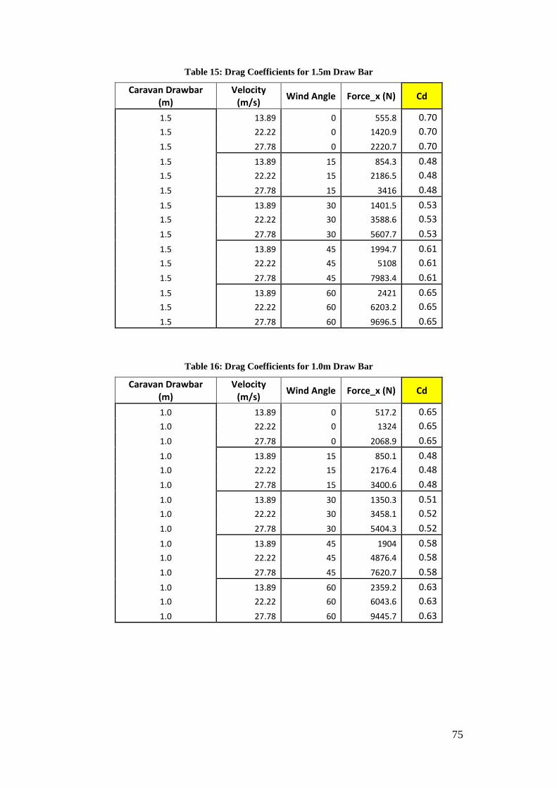
75
Table 15: Drag Coefficients for 1.5m Draw Bar
Caravan Drawbar (m)
Velocity (m/s)
Wind Angle Force_x (N) Cd
1.5 13.89 0 555.8 0.70
1.5 22.22 0 1420.9 0.70
1.5 27.78 0 2220.7 0.70
1.5 13.89 15 854.3 0.48
1.5 22.22 15 2186.5 0.48
1.5 27.78 15 3416 0.48
1.5 13.89 30 1401.5 0.53
1.5 22.22 30 3588.6 0.53
1.5 27.78 30 5607.7 0.53
1.5 13.89 45 1994.7 0.61
1.5 22.22 45 5108 0.61
1.5 27.78 45 7983.4 0.61
1.5 13.89 60 2421 0.65
1.5 22.22 60 6203.2 0.65
1.5 27.78 60 9696.5 0.65
Table 16: Drag Coefficients for 1.0m Draw Bar
Caravan Drawbar (m)
Velocity (m/s)
Wind Angle Force_x (N) Cd
1.0 13.89 0 517.2 0.65
1.0 22.22 0 1324 0.65
1.0 27.78 0 2068.9 0.65
1.0 13.89 15 850.1 0.48
1.0 22.22 15 2176.4 0.48
1.0 27.78 15 3400.6 0.48
1.0 13.89 30 1350.3 0.51
1.0 22.22 30 3458.1 0.52
1.0 27.78 30 5404.3 0.52
1.0 13.89 45 1904 0.58
1.0 22.22 45 4876.4 0.58
1.0 27.78 45 7620.7 0.58
1.0 13.89 60 2359.2 0.63
1.0 22.22 60 6043.6 0.63
1.0 27.78 60 9445.7 0.63

76
Figure 6.1: Drag Coefficients for Modified Caravan Draw Bar
Table 17: Lift Coefficient for 1.8m Draw Bar
Caravan Drawbar (m)
Velocity (m/s)
Wind Angle Force_y (N) CL
1.8 13.89 0 83.8 0.11
1.8 22.22 0 217.5 0.11
1.8 27.78 0 340.6 0.11
1.8 13.89 15 61.7 0.03
1.8 22.22 15 153.2 0.03
1.8 27.78 15 236.1 0.03
1.8 13.89 30 241.2 0.09
1.8 22.22 30 611.4 0.09
1.8 27.78 30 951.4 0.09
1.8 13.89 45 297.3 0.09
1.8 22.22 45 756.5 0.09
1.8 27.78 45 1178.8 0.09
1.8 13.89 60 387.3 0.10
1.8 22.22 60 980.6 0.10
1.8 27.78 60 1524.8 0.10
0.40
0.50
0.60
0.70
0.80
0.90
0 15 30 45 60
CD
Wind Angle (°)
Coefficient of Drag for Draw Bar Configurations
1.8 m Draw Bar
1.5 m Draw Bar
1.0 m Draw Bar

77
Table 18: Lift Coefficient for 1.5m Draw Bar
Caravan Drawbar (m)
Velocity (m/s)
Wind Angle Force_y (N) CL
1.5 13.89 0 80.4 0.10
1.5 22.22 0 206.9 0.10
1.5 27.78 0 324.37 0.10
1.5 13.89 15 120.5 0.07
1.5 22.22 15 305.5 0.07
1.5 27.78 15 475.2 0.07
1.5 13.89 30 209.8 0.08
1.5 22.22 30 533.4 0.08
1.5 27.78 30 830.9 0.08
1.5 13.89 45 360.8 0.11
1.5 22.22 45 921.9 0.11
1.5 27.78 45 1439 0.11
1.5 13.89 60 468.2 0.12
1.5 22.22 60 1196.2 0.12
1.5 27.78 60 1865.6 0.12
Table 19: Lift Coefficient for 1.0m Draw Bar
Caravan Drawbar (m)
Velocity (m/s)
Wind Angle Force_y (N) CL
1.0 13.89 0 60 0.08
1.0 22.22 0 153.4 0.08
1.0 27.78 0 241.4 0.08
1.0 13.89 15 72.9 0.04
1.0 22.22 15 183.8 0.04
1.0 27.78 15 285.1 0.04
1.0 13.89 30 150.6 0.06
1.0 22.22 30 382.9 0.06
1.0 27.78 30 596.5 0.06
1.0 13.89 45 244.8 0.07
1.0 22.22 45 621.7 0.07
1.0 27.78 45 968 0.07
1.0 13.89 60 431.7 0.12
1.0 22.22 60 1097.9 0.11
1.0 27.78 60 1710.2 0.11

78
Figure 6.2: Lift Coefficients for Modified Caravan Draw Bar
Table 20: Side Force Coefficient for 1.8 m Draw Bar
Caravan Drawbar (m)
Velocity (m/s)
Wind Angle Force_z (N) CS
1.8 13.89 0 20 0.03
1.8 22.22 0 56.6 0.03
1.8 27.78 0 89.1 0.03
1.8 13.89 15 628.8 0.36
1.8 22.22 15 1613 0.36
1.8 27.78 15 2522.9 0.36
1.8 13.89 30 1167.5 0.45
1.8 22.22 30 2989.1 0.45
1.8 27.78 30 4673.2 0.45
1.8 13.89 45 1247.3 0.38
1.8 22.22 45 3197.8 0.38
1.8 27.78 45 4999.9 0.38
1.8 13.89 60 1080.6 0.29
1.8 22.22 60 2769.2 0.29
1.8 27.78 60 4328.6 0.29
0.00
0.02
0.04
0.06
0.08
0.10
0.12
0.14
0 15 30 45 60
CL
Wind Angle (°)
Coefficient of Lift for Draw Bar Configurations
1.8 m DrawBar1.5 m DrawBar1.0 m DrawBar

79
Table 21: Side Force Coefficients for 1.5m Draw Bar
Caravan Drawbar (m)
Velocity (m/s)
Wind Angle Force_z (N) CS
1.5 13.89 0 12.1 0.02
1.5 22.22 0 30.7 0.02
1.5 27.78 0 48 0.02
1.5 13.89 15 636.2 0.36
1.5 22.22 15 1631.3 0.36
1.5 27.78 15 2550.6 0.36
1.5 13.89 30 1147 0.44
1.5 22.22 30 2940.2 0.44
1.5 27.78 30 4596.7 0.44
1.5 13.89 45 1307.6 0.40
1.5 22.22 45 3352.7 0.40
1.5 27.78 45 5241.9 0.40
1.5 13.89 60 1128.2 0.30
1.5 22.22 60 2894.2 0.30
1.5 27.78 60 4526.2 0.30
Table 22: Side Force Coefficients for 1.0m Draw Bar
Caravan Drawbar (m)
Velocity (m/s)
Wind Angle Force_z (N) CS
1.0 13.89 0 11.1 0.01
1.0 22.22 0 28.5 0.01
1.0 27.78 0 44.6 0.01
1.0 13.89 15 617.5 0.35
1.0 22.22 15 1584.9 0.35
1.0 27.78 15 2479.1 0.35
1.0 13.89 30 1082.6 0.41
1.0 22.22 30 2776.9 0.41
1.0 27.78 30 4342.6 0.41
1.0 13.89 45 1234.6 0.37
1.0 22.22 45 3163.4 0.37
1.0 27.78 45 4944.5 0.37
1.0 13.89 60 1096.9 0.29
1.0 22.22 60 2811.4 0.29
1.0 27.78 60 4395.2 0.29

80
Figure 6.3: Side Force Coefficients for Modified Caravan Draw Bar
6.3 Geometry Variation
This section discusses the impact that each geometry variation has on the aerodynamic
efficiency of the caravan.
6.3.1 Draw Bar Modification
It is observed through the simulations at a wind speed of 80 km/hr that as the draw bar is
reduced in length the Force in the x direction reduces. The difference between the baseline
length and the 1.0 m Draw bar is 340 N.
When looking at the forces in the y direction it is observed that the 1.0 m draw bar
demonstrates the greatest reduction in lift forces especially at angle between 30° and 45°.
The 1.0 m Draw bar shows it is the better of the options for minimising the side forces in
the z direction. This is amplified at wind angles above 30°.
The full results for the Draw Bar Analysis can be located in Appendix E, F and G.
0.00
0.10
0.20
0.30
0.40
0.50
0 15 30 45 60
CS
Wind Angle (°)
Coefficient of Side Force for Draw Bar Configurations
1.8 m DrawBar1.5 m DrawBar1.0 m DrawBar

81
Figure 6.4: Draw Bar Forces in x Direction
Figure 6.5: Draw Bar Forces in y Direction
Figure 6.6: Draw Bar Forces in z Direction
0
1000
2000
3000
4000
5000
6000
7000
0 15 30 45 60
Forc
e (N
)
Wind Angle
Force in x for Draw Bar Modification
1.8 m Draw Bar
1.5 m Draw Bar
1.0 m Draw Bar
0
200
400
600
800
1000
1200
1400
0 15 30 45 60
Forc
e (N
)
Wind Angle
Force in y for Draw Bar Modification
1.8 m Draw Bar
1.5 m Draw Bar
1.0 m Draw Bar
0
500
1000
1500
2000
2500
3000
3500
4000
0 15 30 45 60
Forc
e (N
)
Wind Angle
Force in z for Draw Bar Modification
1.8 m Draw Bar
1.5 m Draw Bar
1.0 m Draw Bar

82
Figure 6.7: Pressure Distribution on Caravan with 1.0 m Draw Bar
It was observed that as the draw bar was reduced in length, the area on the front of the
caravan that shows the higher pressure distribution shifts vertically. This is due to the
reducing gap between the car and the caravan. The airflow as it leaves the roof of the tow
vehicle strikes higher up the front of the caravan, this reducing the size of the high pressure
contact patch.
6.3.2 Edge Radius Modification
The edge radius modification results show a significant improvement in the streamlining
of the caravan body profile. This initial baseline caravan produced a force in the x direction
of 1436.1 N with an airflow velocity of 80 km/hr and the caravan position directly into the
flow. With the addition of a 100 mm edge radius the force is observed to reduce to 1265.6
N which is a reduction of 170.5 N.
Using the fuel consumption calculation method in Chapter 3, based on proportionality to
the stipulated Land Rover economy figures, this equates to a reduction of 2.6 l/100 km.

83
Figure 6.8: Baseline Caravan Edge Modification Comparison
It is observed that the 350 mm edge radius provides the largest reduction in force figures
under all wind direction configurations. Utilising the 350 mm edge radius on the baseline
caravan provides a 195 N reduction in force.
The rounded edges also serve to provide a smoother transition for the airflow travelling
around the edge. It can be seen from the streamline plot that the air flows past the front
and rear edge of the caravan and stays closer to the surface.
0
1000
2000
3000
4000
5000
6000
7000
0 15 30 45 60
Forc
e (N
)
Wind Angle
Baseline Caravan Edge Modification Force_x Comparison
Baseline
Baseline + 100 mm
Baseline + 350mm

84
Figure 6.9: 350mm Edge at 45° flow
6.3.3 Frontal Vane Modification
The final modification analysed was the inclusion of a vane type assembly to the front of
the caravan. The results demonstrate an even further reduction in force in the x direction.
The final caravan model featuring the 1.0m draw bar with 350mm rounded edges with the
addition of the vane assembly, was simulated under initial conditions of 80 km/hr air flow
at 0° Yaw. The results show a force of 1170 N which is a reduction of 266 N over the
initial baseline caravan.
The streamline plot show in addition to the airflow conforming to the rounded edges, part
of the airflow becomes trapped between the outer vanes and a rotational flow is created as
it makes its way up the front surface of the caravan and spills over the roof.

85
Figure 6.10: Velocity Streamlines of Final Caravan Design
6.4 Fuel Efficiency Calculations
Based on the reduction of 266 N in the x direction over the baseline configuration, the
following estimate can be made regarding the theoretical improvement in fuel economy of
the tow vehicle. Given that the calculations are based on proportionality to the established
data and not based on engine power curves and other specific details regarding the tow
vehicle, it is recommended that a more detailed assessment be made regarding other
contributing factors.
Original Force for Baseline Caravan: 1436.1 N
Optimised Caravan (1.0 m Draw Bar, 350 mm Edge & Frontal Vane): 1170.4 N
Landrover Force_x: 568 N
Original Calculated Fuel Economy of Tow Vehicle with Baseline Caravan: 22.2 l/100 km
Therefore: 1170.4
568× 8.8 = 18.1 𝐿/100𝑘𝑚
Reduction of 4.1 l/100km
86
CHAPTER 7 - CONCLUSION
7.1 Overview
This final chapter discusses the findings of this study and presents some guiding
recommendations to the implementation of the modifications explored during the
optimisation study. It also introduces future work to consider in order to validate these
results. Detailed within are also limitations encountered during the study and
recommendations on how to possibly address them.
7.2 Conclusions
In line with Project Specification, this study progressed through various important stages
resulting in the final results being obtained, regarding the improvement of the caravan
design by modelling crosswind flow. The important first stage was to understand the
problem statement as provided by the Engineering Faculty at USQ. Once understood the
project moved into undertaking a literature review regarding crosswind flow effects on
vehicles. It was noted very early on that there was limited literature on optimising caravan
designs that focussed on crosswind effects. Reviewing the effects of crosswinds on other
transportation methods allowed for parallel to be drawn that would be relevant to the tow
vehicle caravan scenario. The importance of understanding CFD methods was critical to
the undertaking of this project.
Following the literature models of the tow vehicle and caravan were produced for use in
the CFD simulation. The initial study conducted on the baseline caravan allowed for some
important data to be collected which would later be used to compare against the modified
results. The parametric study focused carrying out modifications to the caravan in order to
validate their effectiveness through CFD.
The results obtained showed that there was scope to improve the caravan’s aerodynamic
properties by up to 18% which preliminary calculations indicate could enhance the tow
vehicles fuel economy whilst towing by approximately 4 litres per hundred kilometres of
driving.
These results are promising keeping in mind that further work would need to be carried
out to assess the practicality of the final design.

87
7.3 Limitations and Future Work
Two limitations identified during the early stages of this study involve the modelling of
tow vehicle and caravan and the meshing used in the CFD simulations. The three
dimensional models created could have been created with greater accuracy however it was
decided that due to high computing requirements in meshing the models were simplified.
It is expected that the models would produce less accurate results however it was decided
that this would be acceptable for this study.
The meshing quality was also experimented with and was subsequently reduced in order
to manage the time available for simulation. It would be possible using a high end
computer processor to handle these computations efficiently with an expected increase in
accuracy.
As detailed in the Project Specification there is scope for performing the simulations using
transient wind loading as would be expected in normal every day driving.
In order to validate the results obtained through the CFD analysis it would be expected
that scale models would be produced and tested in a wind tunnel, to obtain force figures
for comparison. The wind tunnel could also be used to perform particle image velocimetry
in order to capture the flow lines around the model.
In addition the expansion of this study to carry out an analysis of the dynamic response of
the caravan to the wind would be beneficial in order to assess vehicle handling and safety
issues.

88
LIST OF REFERENCES
Aerodynamics, 2011 Swift Group Caravans, United Kingdom, viewed 18 March 2016,
<swiftrv.com.au/wp-content/uploads/2013/01/CFD_study.pdf>
Asress, MB & Svorcan, J 2014, 'Numerical investigation on the aerodynamic
characteristics of high-speed train under turbulent crosswind', Journal of Modern
Transportation, vol. 22, no. 4, pp. 225-234, http://dx.doi.org/10.1007/s40534-014-0058-7
Bakker, A, 2002, ‘Applied Computational Fluid Dynamics’, Lecture 7 Meshing, viewed
14 June 2016, www.bakker.org
Basson, J 2013, ‘Analysis of the aerodynamic attributes of motor vehicles’, B.Eng thesis,
University of Southern Queensland, Toowoomba.
Briskey, K 2013, ‘Improving Caravan Design by Modelling of Airflow’, B.Eng thesis,
University of Southern Queensland, Toowoomba.
Cambridge Dictionary, 2016, Crosswind, Cambridge University Press, viewed 08 May
2016, <http://dictionary.cambridge.org/dictionary/english/crosswind>
Carfolio, 2013, LandRover Discovery Specifications, viewed 03 May 2016,
<http://www.carfolio.com/specifications/models/?man=6801>
Engineers Australia 2016, Western Australia Division, Engineers Australia–Code of
Ethics, viewed 13 May 2016, <https://www.engineersaustralia.org.au/western-australia-
division/code-ethics>
ERP 2016, Project Specification, Improving Caravan Design by Modelling of Airflow,
University of Southern Queensland, viewed 5 March 2016,
<http://usqstudydesk.usq.edu.au/m2/pluginfile.php/641537/mod_resource/content/2/V2/
ProjectListAll-auto.html>
Feasibility Study into the Aerodynamic Improvement of Caravans, Gleyndwr University,
Wales, viewed 12 March 2016,
http://www.astutewales.com/en/getfile.php?type=site_documents&id=31.%20Case%20S
tudy%20Fifth%20Wheel%20(updated%2019_06_2014).pdf
Frei, W, 2013, Comsol Blog, ‘Introduction to Turbulence Modelling’, viewed 18 July
2016, https://www.comsol.com/blogs/which-turbulence-model-should-choose-cfd-
High Speed Rail History, 2015, UIC, France, viewed 04 May 2016,
<http://www.uic.org/High-Speed-History>

89
Hillocks, M 2015, ‘Design of a Low Drag Caravan’,B.Eng thesis, University of Southern
Queensland, Toowoomba.
Johnson, FT, Tinoco, EN & Yu, NJ 2005, 'Thirty years of development and application of
CFD at Boeing Commercial Airplanes, Seattle', Computers & Fluids, vol. 34, no. 10, pp.
1115-1151, <http://www.sciencedirect.com/science/article/pii/S0045793005000125>
Johnston, D,U.S Centennial of Flight Commission , Early Developments in
Aerodynamics, viewed 10 May 2016,
http://www.centennialofflight.net/essay/Theories_of_Flight/early_aero/TH3.htm
Keating, M, 2010 , Strategies to Achieve Reliable and Accurate CFD Solutions, ANSYS
UK.
Kee, JD, Rho, JH, Kim, KH & Lee, DH 2014, 'High speed driving stability of passenger
car under crosswind effects', International Journal of Automotive Technology, vol. 15, no.
5, pp. 741-747, http://dx.doi.org/10.1007/s12239-014-0077-8
Kuron, M , 2015, 3 Criteria for assessing CFD Convergence, viewed 12 June 2016,
http://www.engineering.com/DesignSoftware/DesignSoftwareArticles/ArticleID/9296/3-
Criteria-for-Assessing-CFD-Convergence.aspx
Kuzmin, D, 2012, Lecture Notes – Introduction to Computational Fluid Dynamics,
University of Dortmund, accessed 12 June 2016, http://www.mathematik.uni-
dortmund.de/~kuzmin/cfdintro/lecture1.pdf
Discovery 4 Specification Sheet, Land Rover 2016,
http://www.landrover.com.au/vehicles/discovery4/index.html
Malviya, V , Gundala, M and Mishra, R, 2009, Effect of Crosswind on Aerodynamic
Coefficients of Ground Vehicles, University of Huddersfield ,pp. 19-20.
Mansor, S., Rahman, M.R. and Passmore, M.A., Dynamic Simulation of Vehicle
Crosswind Sensitivity for Various Rear Slant Angle.
Mass Production of Cars, 2016, Dorling Kindersley Limited, England, viewed 03 June
2016, http://www.dkfindout.com/uk/transport/history-cars/mass-production/
NTI’s Guide to the Trucking Industry, National Transport Insurance, 2011, viewed 17
August 2016, https://www.nti.com.au/intermediaries/insurance/ntis-guide-to-the-
trucking-industry-2016.php
Pritchard, PJ 2011, Fox and McDonald’s Introduction to Fluid Mechanics, 8th edn. John
Wiley & Sons, p.207.

90
Suzuki, M, Tanemoto, K & Maeda, T 2003, 'Aerodynamic characteristics of
train/vehicles under cross winds', Journal of Wind Engineering and Industrial
Aerodynamics, vol. 91, no. 1–2, pp. 209-218,
http://www.sciencedirect.com/science/article/pii/S016761050200346X
USQ 2016, ENG4111 Research Project Part 1 Project Reference Book, University of
Southern Queensland, Toowoomba.

91
APPENDICES
Appendix A - Project Specification

92
Appendix B - Project Timelines

93
Appendix C - Risk Assessment
Risk mitigation over certain phases of this research is performed by assessing both the
likelihood and consequence of the potential danger in order to make an assessment of the
hazards presented and decide how to proceed.
Likelihood
Defined as the probability of an event occurring that will lead to a particular consequence.
Likelihood can be categorised into the following five categories in order of likelihood;
1. Rare
2. Unlikely
3. Possible
4. Likely
5. Almost Certain
Likelihood Description Frequency
Almost
certain
Expected to occur in
most circumstances
Likely to occur more than once per
year
Likely Probably occur in most
circumstances
Likely to occur approximately once
per year
Possible Could occur at
sometime
Likely to occur approximately once
every five years
Unlikely Not expected to occur Likely to occur approximately once
every five to ten years
Rare Exceptional
circumstances only
Likely to occur with less frequency
than once every ten years
Table 23: Likelihood Category Table
Consequence
Defined as the outcome of the hazardous event. It is based on the direct effect to the
individual or group.
Consequence is categorised into the following five categories in order of consequence;
1. Negligible

94
2. Minor
3. Moderate
4. Major
5. Severe
Rating Consequence
Severe Death or multiple life threatening injuries.
Major Life threatening injury or multiple serious injuries causing hospitalisation.
Moderate Serious injury causing hospitalisation.
Minor Minor injury requiring medical treatment and / or lost time from the workplace.
Negligible Ailments requiring first aid treatment - minor cuts, bruises, bumps.
Table 24: Consequence Category Table
Both Likelihood and Consequence are used as inputs into a Risk Matrix which is used to
determine the level of risk and subsequently treat the risk as appropriate.
Likelihood Consequence
Negligible Minor Moderate Major Severe
Almost
certain Low Medium High Very High Very High
Likely Low Medium High High Very High
Possible Low Medium Medium High High
Unlikely Low Low Medium Medium High
Rare Low Low Low Medium Medium
Table 25: Risk Management Matrix (Australian Sports Commission)
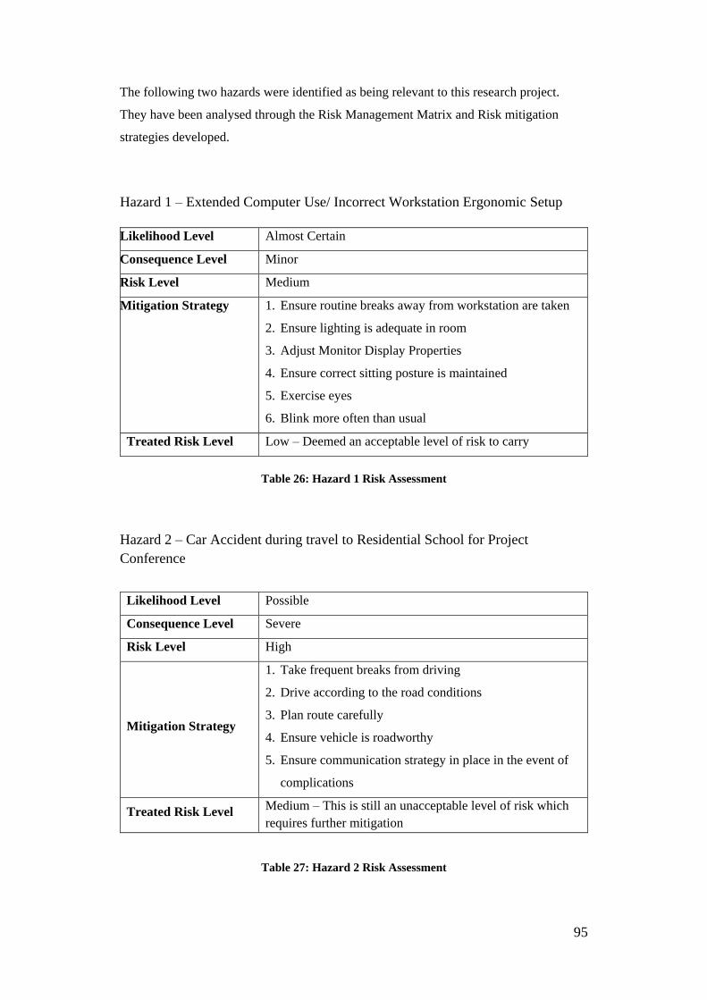
95
The following two hazards were identified as being relevant to this research project.
They have been analysed through the Risk Management Matrix and Risk mitigation
strategies developed.
Hazard 1 – Extended Computer Use/ Incorrect Workstation Ergonomic Setup
Likelihood Level Almost Certain
Consequence Level Minor
Risk Level Medium
Mitigation Strategy 1. Ensure routine breaks away from workstation are taken
2. Ensure lighting is adequate in room
3. Adjust Monitor Display Properties
4. Ensure correct sitting posture is maintained
5. Exercise eyes
6. Blink more often than usual
Treated Risk Level Low – Deemed an acceptable level of risk to carry
Table 26: Hazard 1 Risk Assessment
Hazard 2 – Car Accident during travel to Residential School for Project
Conference
Likelihood Level Possible
Consequence Level Severe
Risk Level High
Mitigation Strategy
1. Take frequent breaks from driving
2. Drive according to the road conditions
3. Plan route carefully
4. Ensure vehicle is roadworthy
5. Ensure communication strategy in place in the event of
complications
Treated Risk Level Medium – This is still an unacceptable level of risk which
requires further mitigation
Table 27: Hazard 2 Risk Assessment
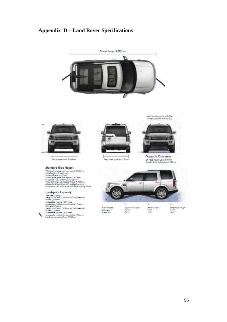
96
Appendix D – Land Rover Specifications

97
Appendix E – Baseline Caravan Data Sheet (1.8 m Draw Bar)
Table 28: Caravan 1.8m Draw Bar Data
DrawBar
Length (m)
Wind Velocity
(m/s)
Speed
(km/h)
Wind
Angle Nodes Elements Force x (N) Force y (N) Force z (N)
Convergence
Iterations
1.8 13.8 50 0 119876 575961 560.3 80.2 19.5 138
1.8 22.22 80 0 119876 575961 1436.1 217.5 56.6 107
1.8 27.77 100 0 119786 575961 2244.4 340.6 89.1 106
1.8 13.8 50 15 119369 573889 876.8 61.7 628.4 87
1.8 22.22 80 15 119369 573889 2244.7 153.2 1613 86
1.8 27.77 100 15 119369 573889 3507.6 236.1 2522.9 86
1.8 13.8 50 30 119688 574918 1434.8 241.2 1166 62
1.8 22.22 80 30 119688 574918 3674.6 611.4 2989.1 64
1.8 27.77 100 30 119688 574918 5742.9 951.4 4673.2 65
1.8 13.8 50 45 110873 537001 2040.4 297.3 1247.3 78
1.8 22.22 80 45 110873 537001 5226.4 756.5 3197.8 78
1.8 27.77 100 45 110873 537001 8168.2 1178.8 4999.9 78
1.8 13.8 50 60 116295 562929 2492.1 387.3 1080.6 75
1.8 22.22 80 60 116295 562929 6383.9 980.6 2769.2 75
1.8 27.77 100 60 116295 562929 9977.7 1524.8 4328.6 75

98
Appendix F - Caravan 1.5 m Draw Bar Data Sheet
Table 29: Caravan 1.5m Draw Bar Data
DrawBar
Length (m)
Wind Velocity
(m/s)
Speed
(km/h)
Wind
Angle Nodes Elements
Force x
(N)
Force y
(N)
Force z
(N) Iter
1.5 13.8 50 0 120028 576721 555.8 80.4 12.1 94
1.5 22.22 80 0 120028 576721 1420.9 206.9 30.4 95
1.5 27.77 100 0 120028 576721 2220.7 324.4 48 100
1.5 13.8 50 15 115175 557118 854.3 120.5 636.2 79
1.5 22.22 80 15 115175 557118 2186.5 305.5 1631.3 79
1.5 27.77 100 15 115175 557118 3416 475.2 2550.6 79
1.5 13.8 50 30 115055 555670 1401.5 209.8 1147 61
1.5 22.22 80 30 115055 555670 3588.6 533.4 2940.2 61
1.5 27.77 100 30 115055 555670 5607.7 830.9 4596.7 61
1.5 13.8 50 45 116200 561722 1994 360.8 1307.6 114
1.5 22.22 80 45 116200 561722 5108 921.9 3352.7 112
1.5 27.77 100 45 116200 561722 7983.4 1439 5241.9 111
1.5 13.8 50 60 119736 578842 2421 468.5 1128.2 124
1.5 22.22 80 60 119736 578842 6203.2 1196.2 2894.2 126
1.5 27.77 100 60 119736 578842 9696.5 1865.6 4526.2 126

99
Appendix G - Caravan 1.0 m Draw Bar Data Sheet
Table 30: Caravan 1.0m Draw Bar Data
DrawBar Length (m)
Wind Velocity
(m/s)
Speed (km/h)
Wind Angle
Nodes Elements Force x
(N) Force y
(N) Force z
(N) Iter
1.0 13.8 50 0 111292 537382 517.2 59.4 11.1 99
1.0 22.22 80 0 111292 537382 1324 153.5 28.5 100
1.0 27.77 100 0 111292 537382 2068.9 241.4 44.6 100
1.0 13.8 50 15 112135 542228 850.1 72.9 617.5 82
1.0 22.22 80 15 112135 542228 2176.4 183.8 1584.9 82
1.0 27.77 100 15 112135 542228 3400.6 285.1 2479.1 82
1.0 13.8 50 30 112664 544693 1350.3 150.6 1082.6 65
1.0 22.22 80 30 112664 544693 3458.1 382.9 2776.9 65
1.0 27.77 100 30 112664 544693 5404.3 596.5 4342.6 65
1.0 13.8 50 45 114354 552521 1904 244.8 1234.6 87
1.0 22.22 80 45 114354 552521 4876.4 621.7 3163.4 87
1.0 27.77 100 45 114354 552521 7620.7 968 4944.5 87
1.0 13.8 50 60 116707 564604 2359.2 431.7 1096.9 109
1.0 22.22 80 60 116707 564604 6043.6 1097.9 2811.4 108
1.0 27.77 100 60 116707 564604 9445.7 1710.2 4395.2 107

100
Appendix H - Caravan 1.8m Draw Bar with Modified Edges
Table 31: Caravan 1.8m Draw Bar with Modified Edge Data
DrawBar Length
(m)
Edge Curvature
(mm)
Wind Velocity
(m/s)
Speed (km/h)
Wind Angle
Nodes Elements Force x
(N) Force y
(N) Force z
(N) Iter
1.8m 100 13.8 50 0 126914 612651 494.3 89.2 15.9 122
1.8m 100 22.22 80 0 126914 612651 1265.6 230.4 40.5 119
1.8m 100 27.77 100 0 126914 612651 1977.6 361.4 63.4 118
1.8m 100 13.8 50 15 125279 605307 773.5 44.3 571.3 80
1.8m 100 22.22 80 15 125279 605307 1979.3 109.9 1464.6 80
1.8m 100 27.77 100 15 125279 605307 3092.1 169.5 2289.7 80
1.8m 100 13.8 50 30 126977 613238 1266.7 200.2 1075.9 75
1.8m 100 22.22 80 30 126977 613238 3242.1 513.1 2759.8 76
1.8m 100 27.77 100 30 126977 613238 5064.8 802.3 4315.2 76
1.8m 100 13.8 50 45 126186 609947 1876.2 258.3 1102.9 124
1.8m 100 22.22 80 45 126186 609947 4805.5 658.1 2827.8 128
1.8m 100 27.77 100 45 126186 609947 7509.6 1026.4 4420.9 129
1.8m 100 13.8 50 60 131071 632977 2231.3 466.9 912.6 79
1.8m 100 22.22 80 60 131071 632977 5713.9 1190.5 2339.3 80
1.8m 100 27.77 100 60 131071 632977 8929.6 1856.4 3657.5 81
1.8m 350 13.8 50 0 116626 563846 484.7 80.9 38.1 100
1.8m 350 22.22 80 0 116626 563846 1240.8 207.2 87.7 101
1.8m 350 27.77 100 0 116626 563846 1938.5 323.7 154.9 101
1.8m 350 13.8 50 15 116177 562091 731.2 99.9 529.2 73
1.8m 350 22.22 80 15 116177 562091 1871.6 254.2 1357.6 73
1.8m 350 27.77 100 15 116177 562091 2924.2 396.3 2123 73
1.8m 350 13.8 50 30 116915 565292 1185.6 197.1 1036.5 66
1.8m 350 22.22 80 30 116915 565292 3035.2 501.5 2657.6 66
1.8m 350 27.77 100 30 116915 565292 4742.6 781.5 4155.4 66
1.8m 350 13.8 50 45 119243 576405 1646.4 336.4 1219.8 70
1.8m 350 22.22 80 45 119243 576405 4216.5 858.8 3127.7 70
1.8m 350 27.77 100 45 119243 576405 6590.6 1337.5 4891.3 71
1.8m 350 13.8 50 60 121870 589494 2031.9 446.2 938.2 95
1.8m 350 22.22 80 60 121870 589494 5202.1 1133.1 2406.5 96
1.8m 350 27.77 100 60 121870 589494 8131.3 1764.4 3764.3 97

101
Appendix I - Caravan 1.5m Draw Bar with Modified Edges
Table 32: Caravan 1.5m Draw Bar with Modified Edge Data
DrawBar Length
(m)
Edge Curvature
(mm)
Wind Velocity
(m/s)
Speed (km/h)
Wind Angle
Nodes Elements Force x
(N) Force y
(N) Force z
(N) Iter
1.5m 100 13.8 50 0 136777 659412 1296.7 230.1 4.7 91
1.5m 100 22.22 80 0 136777 659412 1294.3 228.9 4.6 89
1.5m 100 27.77 100 0 136777 659412 2021.5 358 7.2 90
1.5m 100 13.8 50 15 137118 660991 764.7 79.4 564.1 83
1.5m 100 22.22 80 15 137118 660991 1956.4 196 1445.5 84
1.5m 100 27.77 100 15 137118 660991 3056.3 301 2259.7 85
1.5m 100 13.8 50 30 136501 657094 1229.7 228.1 1031.5 59
1.5m 100 22.22 80 30 136501 657094 3146 583.2 2643.5 59
1.5m 100 27.77 100 30 136501 657094 4914.4 910.6 4132.3 59
1.5m 100 13.8 50 45 137502 661822 1752.7 135.1 1130 101
1.5m 100 22.22 80 45 137502 661822 4487.5 338.6 2896.1 101
1.5m 100 27.77 100 45 137502 661822 7012.1 524.1 4528.1 101
1.5m 100 13.8 50 60 143920 692787 2150.5 495.9 894.2 103
1.5m 100 22.22 80 60 143920 692787 5509 1260.2 2285.1 111
1.5m 100 27.77 100 60 143920 692787 8609.1 1960.4 2567.5 112
1.5m 350 13.8 50 0 124556 600292 491.6 108.2 -3 99
1.5m 350 22.22 80 0 124556 600292 1257 277.2 -8 98
1.5m 350 27.77 100 0 124556 600292 1963.1 432.5 -14 97
1.5m 350 13.8 50 15 124604 599442 717.1 132.2 505.6 100
1.5m 350 22.22 80 15 124604 599442 1834.7 331.8 1297.2 100
1.5m 350 27.77 100 15 124604 599442 2865.9 514.3 2029 99
1.5m 350 13.8 50 30 125430 603880 1124 237.4 965.9 66
1.5m 350 22.22 80 30 125430 603880 2876.9 604.4 2477.4 66
1.5m 350 27.77 100 30 125430 603880 4494.9 942.2 3874.1 66
1.5m 350 13.8 50 45 125430 603880 1124 237.4 965.9 66
1.5m 350 22.22 80 45 125430 603880 2876.9 604.4 2477.4 66
1.5m 350 27.77 100 45 125430 603880 4494.9 942.2 3874.1 66
1.5m 350 13.8 50 60 129267 623763 1832.8 486.7 839.2 80
1.5m 350 22.22 80 60 129267 623763 4689.7 1237.6 2147.4 80
1.5m 350 27.77 100 60 129267 623763 7323.3 1927.9 3354.6 80

102
Appendix J - Caravan 1.0m Draw Bar with Modified Edges
Table 33: Caravan 1.0m Draw Bar with Modified Edge Data
DrawBar Length
(m)
Edge Curvature
(mm)
Wind Velocity
(m/s)
Speed (km/h)
Wind Angle
Nodes Elements Force x
(N) Force y
(N) Force z
(N) Iter
1.0m 100 13.8 50 0 126205 609042 471.7 108 2.4 90
1.0m 100 22.22 80 0 126205 609042 1206.3 278.7 6.3 92
1.0m 100 27.77 100 0 126205 609042 1883.5 436.2 10.1 94
1.0m 100 13.8 50 15 125735 607314 745.7 114.8 551.4 89
1.0m 100 22.22 80 15 125735 607314 1907.4 292.3 1412.6 89
1.0m 100 27.77 100 15 125735 607314 2979.3 456 2207.8 88
1.0m 100 13.8 50 30 125917 608641 1198.9 235.7 1018.3 67
1.0m 100 22.22 80 30 125917 608641 3067.9 605.9 2612 68
1.0m 100 27.77 100 30 125917 608641 4792.6 948.2 4084.5 68
1.0m 100 13.8 50 45 128518 620711 1697.4 127.6 1151.6 73
1.0m 100 22.22 80 45 128518 620711 4345.8 323.2 2953.5 72
1.0m 100 27.77 100 45 128518 620711 6791 501.6 4618.7 72
1.0m 100 13.8 50 60 131019 632689 2093.1 521 923.6 80
1.0m 100 22.22 80 60 131019 632689 5359.6 1329.6 2365.2 82
1.0m 100 27.77 100 60 131019 632689 8375.1 2075 3697.5 82
1.0m 350 13.8 50 0 116350 561171 452.8 111.7 -1 96
1.0m 350 22.22 80 0 116350 561171 1158.6 288.2 -2.8 97
1.0m 350 27.77 100 0 116350 561171 1809.6 451.3 -4.5 98
1.0m 350 13.8 50 15 116232 561045 732.8 242.1 487.1 98
1.0m 350 22.22 80 15 116323 561045 1817.1 492.3 1293.8 97
1.0m 350 27.77 100 15 116323 561045 2837.9 768.3 2022.3 98
1.0m 350 13.8 50 30 117432 567697 1104.7 275.8 944.8 61
1.0m 350 22.22 80 30 117432 567697 2827.3 705 2422 61
1.0m 350 27.77 100 30 117432 567697 4417.3 1110.7 3787.6 61
1.0m 350 13.8 50 45 118239 570695 1524.1 315.7 1135.4 108
1.0m 350 22.22 80 45 118239 570695 3902.6 804.8 2910.3 109
1.0m 350 27.77 100 45 118239 570695 6098.7 1255.4 4550.1 110
1.0m 350 13.8 50 60 121066 584538 1924.2 636 1067.9 83
1.0m 350 22.22 80 60 121066 584538 4929.7 1628 2738.5 83
1.0m 350 27.77 100 60 121066 584538 7705.1 2543.7 4282.2 83

103
Appendix K - Baseline Caravan with Frontal Vane System
Table 34: Frontal Vane System Data
Wind Angle Nodes Elements Force x (N) Force y (N) Force z (N) Convergence
Iterations
0 127913 616718 1170.4 199.6 -35.9 84
15 128041 617914 1789.4 222.3 1427.7 111
30 129411 625684 2891.4 547.6 2526.1 66
45 130492 630090 3966.6 268.3 2851.3 89
60 133744 645976 5124 909 2127.7 102
Figure K1: Residuals for Final Caravan Model with Vanes