improved statistical downscaling of daily precipitation using sdsm platform and data-mining methods

INTERNATIONAL JOURNAL OF CLIMATOLOGYInt. J. Climatol. 33: 2561–2578 (2013)Published online 1 November 2012 in Wiley Online Library(wileyonlinelibrary.com) DOI: 10.1002/joc.3611

Improved statistical downscaling of daily precipitation usingSDSM platform and data-mining methods

H. Tavakol-Davani,a M. Nasserib* and B. Zahraiec

a School of Civil Engineering, University of Tehran, Tehran, Iranb School of Civil Engineering, University of Tehran, Tehran, Iran

c Center of Excellence for Engineering and Management of Civil Infrastructures, School of Civil Engineering, University of Tehran, Tehran,Iran

ABSTRACT: In this paper, an extension of the statistical downscaling model (SDSM), namely data-mining downscalingmodel (DMDM), has been developed. DMDM has the same platform as the most cited statistical downscaling models,namely SDSM and ASD. Multiple linear regression (MLR), ridge regression (RR), multivariate adaptive regression splines(MARS) and model tree (MT) constitute the mathematical core of DMDM. DMDM uses linear basis functions in MARSand linear regression rules in MT to keep the linear structure of SDSM; therefore, all of the SDSM assumptions are alsovalid in DMDM. These methods highlight the effect of data partitioning for meteorological predictors in the downscalingprocedure. Inputs and output of the presented approaches are the same as SDSM and ASD. In the case study of thisresearch, NCEP/NCAR databases have been used for calibration and validation. According to the inherent linearity ofthe methods, suitable predictor selection has been done with stepwise regression as a preprocessing stage. The results ofDMDM have been compared with observed precipitation in 12 rain gauge stations that are scattered in different basins inIran and represent different climate regimes. Comparison between the results of SDSM and DMDM has indicated that thepresented approach can highly improve downscaling efficiency in terms of reproducing monthly standard deviation andskewness for both calibration and validation datasets. Among the proposed methods in DMDM, the results of the casestudy have shown that MT has provided better performances both in modelling occurrence and amount of precipitation.Also, MT is potentially recognized as a powerful diagnostic tool that could extract information in key atmospheric driversaffecting local weather. It also has fewer parameters during dry seasons, in which the number of historical precipitationevents might not be enough for calibrating SDSM model in many arid and semi-arid regions.

KEY WORDS statistical downscaling; data-mining methods; climate change; MARS; model tree

Received 20 January 2012; Revised 14 August 2012; Accepted 25 September 2012

1. Introduction

Future scenarios of climate change are achieved fromglobal circulation models (GCMs) which are the pre-mier meteorological sources for approximating plausiblefuture climate. This information is spatially too coarseto determine regional effects of climate change, and itmust be transformed to finer resolutions to be appli-cable in local analysis. Downscaling approaches depictsuitable methods to extract regional-scale meteorologi-cal variables from GCM outputs. Two general types ofmathematical approaches for downscaling of GCM sim-ulations can be listed as follows:

• Dynamical approaches or regional climate models(Mearns et al., 2003)

• Statistical approaches:

* Correspondence to: M. Nasseri, School of Civil Engineering,University of Tehran, Tehran, Iran. E-mail: [email protected],[email protected]

• Regression-based (empirical) methods (Enke andSpekat, 1997; Faucher et al., 1999; Wilby et al.,1999; Li and Sailor, 2000; Hessami et al., 2008;Raje and Mujumdar, 2011),

• Weather pattern approaches (Bardossy and Plate,1992; Yarnal et al., 2001; Anandhi et al., 2011),

• Stochastic weather generators (Semenov and Bar-row, 1997; Bates et al., 1998).

Because of less preprocessing requirements and com-putational costs, statistical approaches in general andregression-based methods in specific have receivedmore attention among the aforementioned downscal-ing approaches. Among different statistical approaches,regression-based methods are famous for simplicity inimplementation. Different tools have been developed forstatistical downscaling using artificial neural networks(ANNs) (Pasini, 2009; Tomassetti et al., 2009; Mendesand Marengo, 2010; Fistikoglu and Okkan, 2011), k-nearest neighbors (Yates, et al., 2003; Gangopadhyayet al., 2005; Raje and Mujumdar, 2011), support vector

2012 Royal Meteorological Society

2562 H. TAVAKOL-DAVANI ET AL.

machines (SVMs) (Tripathi et al., 2006; Chen et al.,2010) and linear regression (Wilby et al., 2002; Hessamiet al., 2008).

Finding empirical relationships between large- andregional-scale climates is the aim of statistical down-scaling methods. Correlation between GCM-scale mete-orological variables (predictors) and local meteorologicalvariables such as precipitation and temperature (pre-dictands) is the master point of statistical downscalingprocedures. Advantages and disadvantages of statisticaldownscaling methods have been discussed by Hessamiet al. (2008). Statistical downscaling model (SDSM) andautomated statistical downscaling (ASD) are among themost cited statistical/empirical downscaling tools. These

packages implement linear regression to estimate theamount and/or the occurrence of local meteorologicalpredictands; simple linear and ridge regression (RR)methods are the mathematical kernels of SDSM andASD, respectively. SDSM and ASD behave well in keep-ing mean of predictands, but they are weak in simulat-ing standard deviation and extreme values (Wilby et al.,2004; Hessami et al., 2008).

In this paper, SDSM (Wilby et al., 2002) and ASD(Hessami et al., 2008) models have been extended usingtwo linear data-mining (DM) methods of model tree (MT)and multivariate adaptive regression splines (MARS).The main reason of using these DM methods is thelinearity of their mathematical kernels, which make them

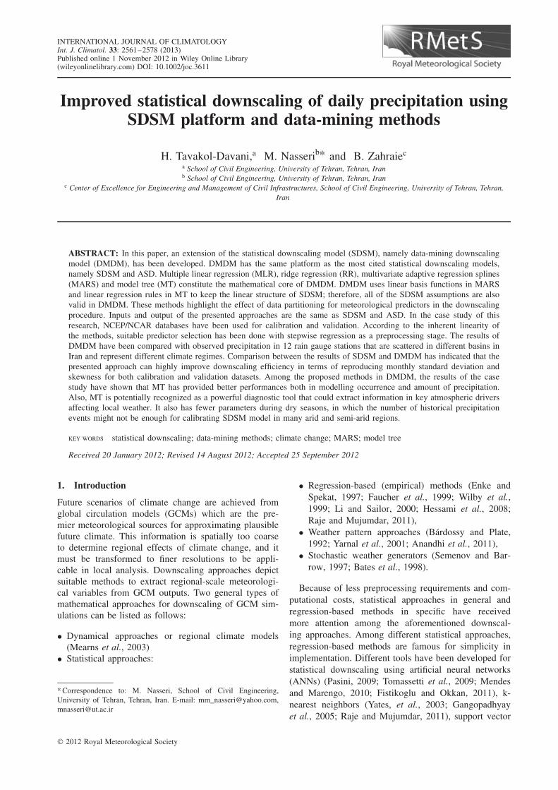
Figure 1. Location map of rain gauges of interest in the five catchments (Jazmoorian, Sefidrood, Mordab-anzali, Shapoor-dalky and Mond basin).

2012 Royal Meteorological Society Int. J. Climatol. 33: 2561–2578 (2013)

SDSM, DATA-MINING METHODS, CLIMATE CHANGE 2563

consistent with SDSM and ASD. DM methods performwell in the regression field, and therefore it is anticipatedthat MT and MARS might outperform multiple linearregression (MLR) and RR in statistical downscaling ofGCM simulations.

In the next section (Section 2), the study areas havebeen described. In Section 3, the platform of SDSMsoftware, MT, MARS and the proposed approach arepresented. Later, in Section 4, the downscaling resultsare presented. In the last section (Section 5), concludingremarks are presented.

2. Case study

2.1. Local data

The selected rain gauge stations in this research arescattered in five basins namely Hamoon-Jazmoorian,Sefidrood, Mordab-Anzali, Shapoor-dalky and Mondwith areas of 69 801, 60 746, 3 224, 21 447 and 47 776km2, respectively. Hamoon-Jazmoorian is located in anarid region in southeast of Iran near Iran–Pakistan bor-der. Sefidrood and Mordab-Anzali basins are located ina wet region in north of Iran near Caspian Sea andShapoor-dalky and Mond basins are located in a rel-atively arid region in southwest of Iran near PersianGulf. These basins are selected based on availabilityof observed meteorological data and also they repre-sent various climatic and hydrologic conditions. Twelverain gauge stations in these basins have been selected(Figure 1). Approximately in all stations, dry and wetseasons are in the periods of May through October andNovember through April, respectively.

According to Table 1, 26–35 years of daily precip-itation records are available for these stations. In thisstudy, the first 75% of recorded datasets is used for cal-ibration and the last 25% is used for validation in eachstation. Daily records of precipitation are collected fromthe national database of the Iranian Ministry of Energy.

2.2. Large-scale datasets

In this research, the outputs of Hadley Center’s GCM(HadCM3) have been utilized. The special reporton emission scenarios (SRES), A2 and B2 scenarioshave been used to project the future climate con-ditions. Large-scale NCEP reanalysis atmosphericdata (Table 1) have been used as the model predic-tors. Spatial resolution (dimensions of grid box) ofHadCM3 outputs is 3.75◦ (long.) × 2.5◦(lat.), whereasit is 2.5◦(long.) × 2.5◦(lat.) for NCEP data. Therefore,projected large-scale predictors of NCEP on HadCM3computational grid box have been used. These data andHadCM3 daily simulations are supported and distributedby the Canadian Climate Change Scenarios Network(CCCSN) (http://www.cccsn.ec.gc.ca) and also theCanadian Climate Impacts Scenarios (CCIS) website(www.cics.uvic.ca/scenarios/sdsm/select.cgi). There are26 different atmospheric variables for each grid box inthis database. For each rain gauge station, nine boxescovering the study areas have been selected. Figure 1depicts centre of each meteorological grid box and loca-tion of the selected rain gauge stations. As it can be seenin this figure, the grid boxes cover a large area over theselected basins and around them. In addition, 1- to 3-dlagged series of the predictors have also been consideredas new predictors in this research. For each station, 828(9 (no. of boxes) × 23 (atmospheric variables) × 4 (num-ber of lags)) predictors have been analyzed, which areexplained in more details in the next sections of the paper.

3. Methodology

3.1. Statistical downscaling model

SDSM software is developed based on multiple lin-ear regression downscaling model (MLRDM). SDSMpresents several weather ensembles and its outputs arethe average of these ensembles. These ensembles are theresults of linear regression models with stochastic terms

Table 1. Basic information about 12 raingauges.

Statistical characteristics ofobserved daily rainfall (mm)

No. Stationcode

Stationname

Abbr. Basin Length ofdataset (year)

Longitude(◦E)

Latitude(◦N)

Mean Max. Std.

1 44-009 Dehrood Deh. Jazmoorian 1975–2000 57.73 28.87 0.76 132 4.712 44-014 Delfard Del. Jazmoorian 57.60 29.00 1.20 150 6.313 44-016 Khoramshahi Kho. Jazmoorian 57.75 29.00 1.32 194 6.954 44-024 Kharposht Kha. Jazmoorian 57.83 28.48 0.46 80 3.205 17-075 Farshekan Far. Sefidrood 1966–2000 49.58 37.40 3.30 168 9.936 17-082 Rasht Ras. Sefidrood 49.60 37.25 3.58 188 10.347 18-007 Kasma Kas. Mordab-anzali 49.30 37.31 3.01 317 9.598 18-017 Shanderman Shan. Mordab-anzali 49.11 37.41 2.67 177 8.239 23-011 Shapoor Shap. Shapoor-dalky 1972–2000 51.11 29.58 0.85 75 4.4510 23-019 Shoorjareh Shoo. Shapoor-dalky 51.98 29.25 0.99 120 4.9211 43-034 Arsanjan Ars. Shapoor-dalky 51.30 29.92 0.87 111 4.5612 24-033 Khanzanian Khan. Mond 52.15 29.67 1.27 92 5.26

Max., maximum; Std., standard deviation.



d

g p p p g

p p ds

m

m

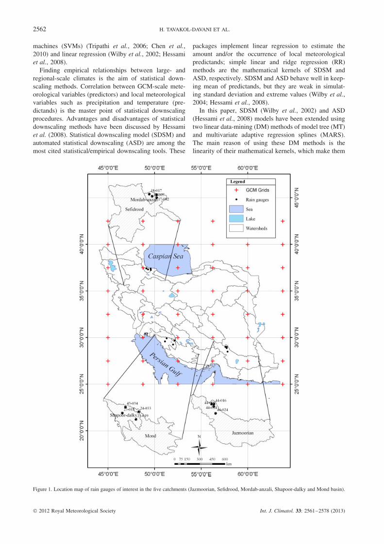
Figure 2. SDSM structure (after Wilby et al., 2002).

of bias correction. The general platform of SDSM hasbeen shown in Figure 2 (Wilby et al., 2002). Because ofthe linear concepts of SDSM, selection of the predictorsis based on the correlation or partial correlation analysisbetween the interested predictand and the predictors andweights of the predictors which are estimated via ordinaryleast-square method. In addition of ordinary least-squaremethod, dual simplex method has been also provided inSDSM for calibration because of instability of regressioncoefficients for nonorthogonal predictor vectors. Hessamiet al. (2008) added a new option of using RR (Hoerland Kennard, 1970) in their downscaling model, namelyASD as a remedy of the nonorthogonality impact of thepredictor vectors.

SDSM model contains two separate sub-modelsto determine occurrence and amount of conditionalmeteorological variables (or discrete variables) such

as precipitation and amount model for unconditionalvariables (or continues variables) such as temperatureor evaporation. Therefore, SDSM can be classified asa conditional weather generator in which regressionequations are used to estimate the parameters of dailyprecipitation occurrence and amount, separately, so itis slightly more sophisticated than a straightforwardregression model. Statistical downscaling using SDSMconsists of the following steps:

1. In first step, suitable predictors should be selected.SDSM provides the ability of some statistical analysisfor users to select the best predictors. In SDSM,predictors should have acceptable unconditional andconditional correlations with the predictand. Also,partial correlation, P -value and explained variance ofthe predictors can be checked while using SDSM.

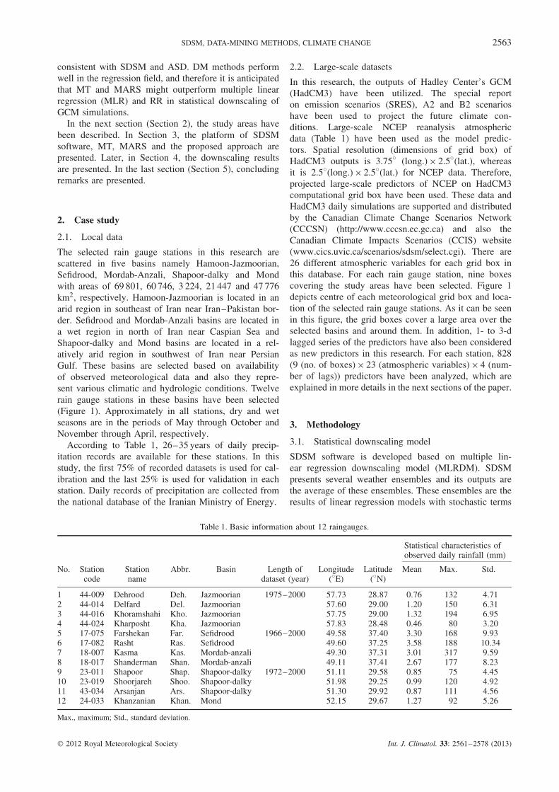
Figure 3. DMDM procedure.



Acceptable ranges for these statistics are proposed byWilby et al. (2004).The scatter plot is another toolprovided in SDSM in order to select the appropriatepredictors.

2. A MLR model is calibrated to simulate the pre-cipitation occurrence which is called unconditionalmodel. This model can be calibrated by two differ-ent methods namely ordinary least-square and dualsimplex methods. An autoregressive term can beadded to this model. For each month, one MLRmodel must be calibrated for occurrence estimation.The days with and without events (precipitation) arerepresented with 1 and 0, respectively. For eachday and ensemble, a uniformly distributed randomnumber between 0 and 1 is generated. If the ran-dom number is less than the output of the occurrencemodel in that day, precipitation occurs. Otherwise,precipitation does not occur.

3. Another MLR model, namely conditional model, iscalibrated to simulate the precipitation amount. Thismodel is calibrated using the available rainy daysdataset. Like the unconditional model, SDSM cali-brate different conditional models for 12 months ofyear. For a day which is identified as a rainy day inthe previous step, output of the amount model is cal-culated. Then, a random number is added to the outputto consider the modelling error. This random numberis generated using a normal distribution function withzero mean and standard deviation equal to standarderror.

4. The result of the previous step is compared with apredefined threshold. If the result is less than thethreshold, the precipitation will not occur. Otherwise,the result is considered as the rainfall amount in thatday and in that ensemble.

(a)

(b)

(c)

(d)

Figure 4. Comparison of SDSM and MLRDM in Del. rain gauge. (a) Monthly mean, (b) monthly standard deviation, (c) monthly skewness and(d) q–q plot (Left column: calibration period, right column: validation period).



Table 2. Large-scale Predictors from NCEP database.

No. Predictor Abbreviation

1 Mean sea level pressure mslp2 Surface airflow strength p__f3 Surface zonal velocity p__u4 Surface meridional velocity p__v5 Surface vorticity p__z6 Surface divergence p_zh7 500 hPa airflow strength p5_f8 500 hPa zonal velocity p5_u9 500 hPa meridional velocity p5_v10 500 hPa vorticity p5_z11 500 hPa bivergence p5zh12 850 hPa airflow strength p8_f13 850 hPa zonal velocity p8_u14 850 hPa meridional velocity p8_v15 850 hPa vorticity p8_z16 850 hPa divergence p8zh17 500 hPa geopotential height p50018 850 hPa geopotential height p85019 Relative humidity at 500 hPa r50020 Relative humidity at 850 hPa r85021 Near surface relative humidity rhum22 Near surface specific humidity shum23 Mean temperature at 2 m temp

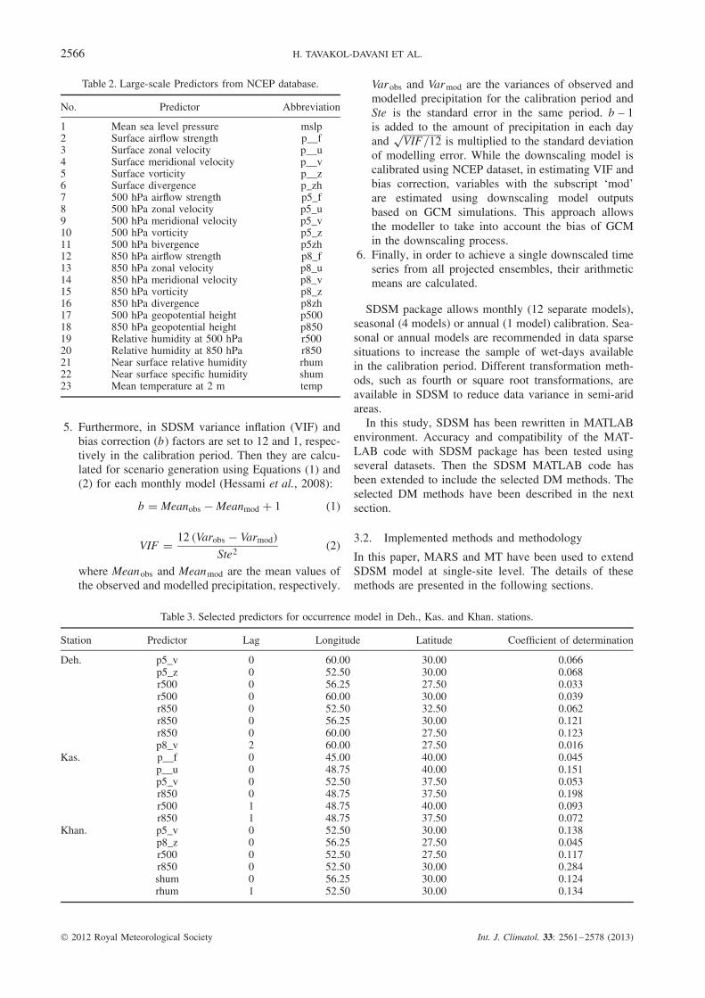
5. Furthermore, in SDSM variance inflation (VIF) andbias correction (b) factors are set to 12 and 1, respec-tively in the calibration period. Then they are calcu-lated for scenario generation using Equations (1) and(2) for each monthly model (Hessami et al., 2008):

b = Meanobs − Meanmod + 1 (1)

VIF = 12 (Varobs − Varmod)

Ste2(2)

where Meanobs and Meanmod are the mean values ofthe observed and modelled precipitation, respectively.

Varobs and Varmod are the variances of observed andmodelled precipitation for the calibration period andSte is the standard error in the same period. b – 1is added to the amount of precipitation in each dayand

√VIF/12 is multiplied to the standard deviation

of modelling error. While the downscaling model iscalibrated using NCEP dataset, in estimating VIF andbias correction, variables with the subscript ‘mod’are estimated using downscaling model outputsbased on GCM simulations. This approach allowsthe modeller to take into account the bias of GCMin the downscaling process.

6. Finally, in order to achieve a single downscaled timeseries from all projected ensembles, their arithmeticmeans are calculated.

SDSM package allows monthly (12 separate models),seasonal (4 models) or annual (1 model) calibration. Sea-sonal or annual models are recommended in data sparsesituations to increase the sample of wet-days availablein the calibration period. Different transformation meth-ods, such as fourth or square root transformations, areavailable in SDSM to reduce data variance in semi-aridareas.

In this study, SDSM has been rewritten in MATLABenvironment. Accuracy and compatibility of the MAT-LAB code with SDSM package has been tested usingseveral datasets. Then the SDSM MATLAB code hasbeen extended to include the selected DM methods. Theselected DM methods have been described in the nextsection.

3.2. Implemented methods and methodology

In this paper, MARS and MT have been used to extendSDSM model at single-site level. The details of thesemethods are presented in the following sections.

Table 3. Selected predictors for occurrence model in Deh., Kas. and Khan. stations.

Station Predictor Lag Longitude Latitude Coefficient of determination

Deh. p5_v 0 60.00 30.00 0.066p5_z 0 52.50 30.00 0.068r500 0 56.25 27.50 0.033r500 0 60.00 30.00 0.039r850 0 52.50 32.50 0.062r850 0 56.25 30.00 0.121r850 0 60.00 27.50 0.123p8_v 2 60.00 27.50 0.016

Kas. p__f 0 45.00 40.00 0.045p__u 0 48.75 40.00 0.151p5_v 0 52.50 37.50 0.053r850 0 48.75 37.50 0.198r500 1 48.75 40.00 0.093r850 1 48.75 37.50 0.072

Khan. p5_v 0 52.50 30.00 0.138p8_z 0 56.25 27.50 0.045r500 0 52.50 27.50 0.117r850 0 52.50 30.00 0.284shum 0 56.25 30.00 0.124rhum 1 52.50 30.00 0.134



(a)

(b)

(c)

(d)

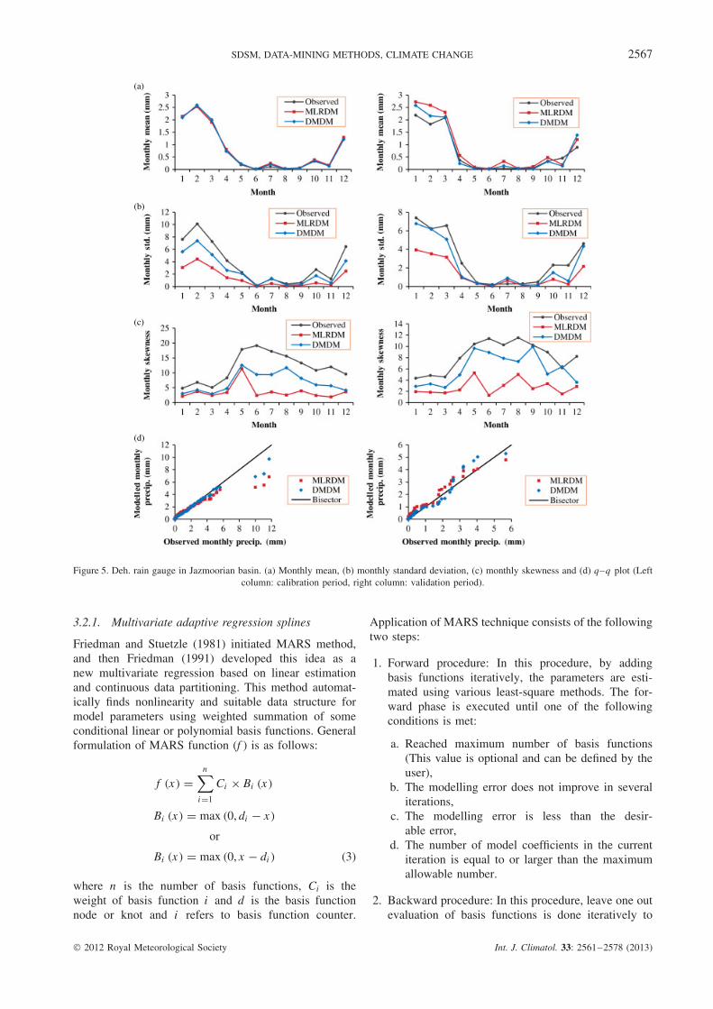
Figure 5. Deh. rain gauge in Jazmoorian basin. (a) Monthly mean, (b) monthly standard deviation, (c) monthly skewness and (d) q–q plot (Leftcolumn: calibration period, right column: validation period).

3.2.1. Multivariate adaptive regression splines

Friedman and Stuetzle (1981) initiated MARS method,and then Friedman (1991) developed this idea as anew multivariate regression based on linear estimationand continuous data partitioning. This method automat-ically finds nonlinearity and suitable data structure formodel parameters using weighted summation of someconditional linear or polynomial basis functions. Generalformulation of MARS function (f ) is as follows:

f (x) =n∑

i=1

Ci × Bi (x)

Bi (x) = max (0, di − x)

or

Bi (x) = max (0, x − di ) (3)

where n is the number of basis functions, Ci is theweight of basis function i and d is the basis functionnode or knot and i refers to basis function counter.

Application of MARS technique consists of the followingtwo steps:

1. Forward procedure: In this procedure, by addingbasis functions iteratively, the parameters are esti-mated using various least-square methods. The for-ward phase is executed until one of the followingconditions is met:

a. Reached maximum number of basis functions(This value is optional and can be defined by theuser),

b. The modelling error does not improve in severaliterations,

c. The modelling error is less than the desir-able error,

d. The number of model coefficients in the currentiteration is equal to or larger than the maximumallowable number.

2. Backward procedure: In this procedure, leave one outevaluation of basis functions is done iteratively to



(a)

(b)

(c)

(d)

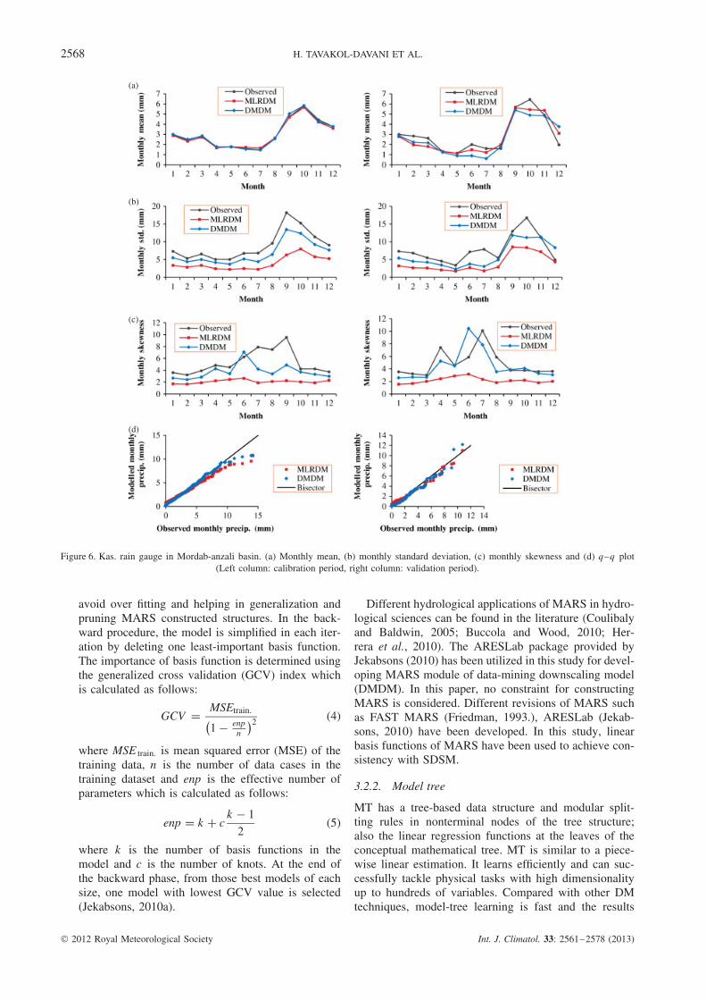
Figure 6. Kas. rain gauge in Mordab-anzali basin. (a) Monthly mean, (b) monthly standard deviation, (c) monthly skewness and (d) q–q plot(Left column: calibration period, right column: validation period).

avoid over fitting and helping in generalization andpruning MARS constructed structures. In the back-ward procedure, the model is simplified in each iter-ation by deleting one least-important basis function.The importance of basis function is determined usingthe generalized cross validation (GCV) index whichis calculated as follows:

GCV = MSEtrain.(1 − enp

n

)2 (4)

where MSE train. is mean squared error (MSE) of thetraining data, n is the number of data cases in thetraining dataset and enp is the effective number ofparameters which is calculated as follows:

enp = k + ck − 1

2(5)

where k is the number of basis functions in themodel and c is the number of knots. At the end ofthe backward phase, from those best models of eachsize, one model with lowest GCV value is selected(Jekabsons, 2010a).

Different hydrological applications of MARS in hydro-logical sciences can be found in the literature (Coulibalyand Baldwin, 2005; Buccola and Wood, 2010; Her-rera et al., 2010). The ARESLab package provided byJekabsons (2010) has been utilized in this study for devel-oping MARS module of data-mining downscaling model(DMDM). In this paper, no constraint for constructingMARS is considered. Different revisions of MARS suchas FAST MARS (Friedman, 1993.), ARESLab (Jekab-sons, 2010) have been developed. In this study, linearbasis functions of MARS have been used to achieve con-sistency with SDSM.

3.2.2. Model tree

MT has a tree-based data structure and modular split-ting rules in nonterminal nodes of the tree structure;also the linear regression functions at the leaves of theconceptual mathematical tree. MT is similar to a piece-wise linear estimation. It learns efficiently and can suc-cessfully tackle physical tasks with high dimensionalityup to hundreds of variables. Compared with other DMtechniques, model-tree learning is fast and the results



(a)

(b)

(c)

(d)

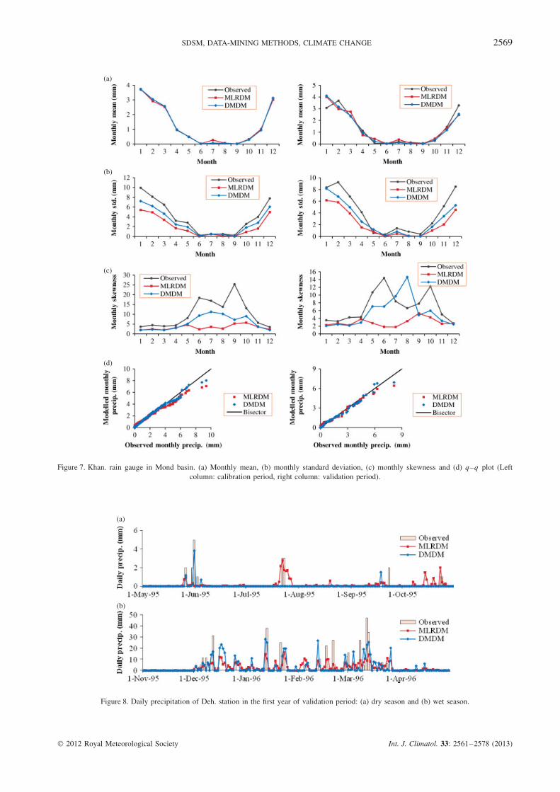
Figure 7. Khan. rain gauge in Mond basin. (a) Monthly mean, (b) monthly standard deviation, (c) monthly skewness and (d) q–q plot (Leftcolumn: calibration period, right column: validation period).

(a)

(b)

Figure 8. Daily precipitation of Deh. station in the first year of validation period: (a) dry season and (b) wet season.



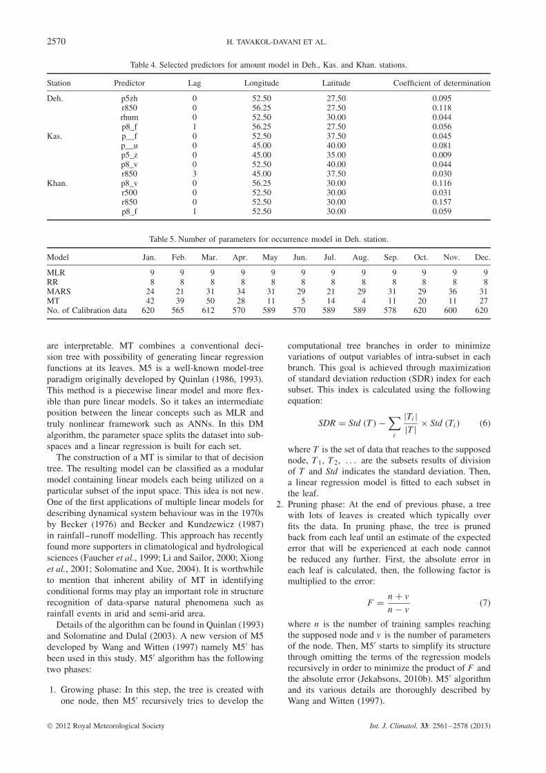
Table 4. Selected predictors for amount model in Deh., Kas. and Khan. stations.

Station Predictor Lag Longitude Latitude Coefficient of determination

Deh. p5zh 0 52.50 27.50 0.095r850 0 56.25 27.50 0.118rhum 0 52.50 30.00 0.044p8_f 1 56.25 27.50 0.056

Kas. p__f 0 52.50 37.50 0.045p__u 0 45.00 40.00 0.081p5_z 0 45.00 35.00 0.009p8_v 0 52.50 40.00 0.044r850 3 45.00 37.50 0.030

Khan. p8_v 0 56.25 30.00 0.116r500 0 52.50 30.00 0.031r850 0 52.50 30.00 0.157p8_f 1 52.50 30.00 0.059

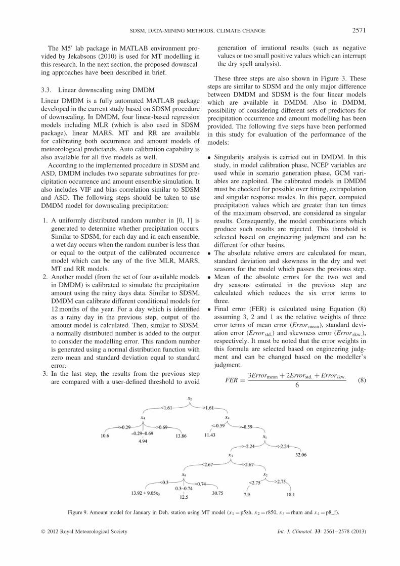
Table 5. Number of parameters for occurrence model in Deh. station.

Model Jan. Feb. Mar. Apr. May Jun. Jul. Aug. Sep. Oct. Nov. Dec.

MLR 9 9 9 9 9 9 9 9 9 9 9 9RR 8 8 8 8 8 8 8 8 8 8 8 8MARS 24 21 31 34 31 29 21 29 31 29 36 31MT 42 39 50 28 11 5 14 4 11 20 11 27No. of Calibration data 620 565 612 570 589 570 589 589 578 620 600 620

are interpretable. MT combines a conventional deci-sion tree with possibility of generating linear regressionfunctions at its leaves. M5 is a well-known model-treeparadigm originally developed by Quinlan (1986, 1993).This method is a piecewise linear model and more flex-ible than pure linear models. So it takes an intermediateposition between the linear concepts such as MLR andtruly nonlinear framework such as ANNs. In this DMalgorithm, the parameter space splits the dataset into sub-spaces and a linear regression is built for each set.

The construction of a MT is similar to that of decisiontree. The resulting model can be classified as a modularmodel containing linear models each being utilized on aparticular subset of the input space. This idea is not new.One of the first applications of multiple linear models fordescribing dynamical system behaviour was in the 1970sby Becker (1976) and Becker and Kundzewicz (1987)in rainfall–runoff modelling. This approach has recentlyfound more supporters in climatological and hydrologicalsciences (Faucher et al., 1999; Li and Sailor, 2000; Xionget al., 2001; Solomatine and Xue, 2004). It is worthwhileto mention that inherent ability of MT in identifyingconditional forms may play an important role in structurerecognition of data-sparse natural phenomena such asrainfall events in arid and semi-arid area.

Details of the algorithm can be found in Quinlan (1993)and Solomatine and Dulal (2003). A new version of M5developed by Wang and Witten (1997) namely M5′ hasbeen used in this study. M5′ algorithm has the followingtwo phases:

1. Growing phase: In this step, the tree is created withone node, then M5′ recursively tries to develop the

computational tree branches in order to minimizevariations of output variables of intra-subset in eachbranch. This goal is achieved through maximizationof standard deviation reduction (SDR) index for eachsubset. This index is calculated using the followingequation:

SDR = Std (T ) −∑

i

|Ti ||T | × Std (Ti ) (6)

where T is the set of data that reaches to the supposednode, T 1, T 2, . . . are the subsets results of divisionof T and Std indicates the standard deviation. Then,a linear regression model is fitted to each subset inthe leaf.

2. Pruning phase: At the end of previous phase, a treewith lots of leaves is created which typically overfits the data. In pruning phase, the tree is prunedback from each leaf until an estimate of the expectederror that will be experienced at each node cannotbe reduced any further. First, the absolute error ineach leaf is calculated, then, the following factor ismultiplied to the error:

F = n + v

n − v(7)

where n is the number of training samples reachingthe supposed node and v is the number of parametersof the node. Then, M5′ starts to simplify its structurethrough omitting the terms of the regression modelsrecursively in order to minimize the product of F andthe absolute error (Jekabsons, 2010b). M5′ algorithmand its various details are thoroughly described byWang and Witten (1997).



The M5′ lab package in MATLAB environment pro-vided by Jekabsons (2010) is used for MT modelling inthis research. In the next section, the proposed downscal-ing approaches have been described in brief.

3.3. Linear downscaling using DMDM

Linear DMDM is a fully automated MATLAB packagedeveloped in the current study based on SDSM procedureof downscaling. In DMDM, four linear-based regressionmodels including MLR (which is also used in SDSMpackage), linear MARS, MT and RR are availablefor calibrating both occurrence and amount models ofmeteorological predictands. Auto calibration capability isalso available for all five models as well.

According to the implemented procedure in SDSM andASD, DMDM includes two separate subroutines for pre-cipitation occurrence and amount ensemble simulation. Italso includes VIF and bias correlation similar to SDSMand ASD. The following steps should be taken to useDMDM model for downscaling precipitation:

1. A uniformly distributed random number in [0, 1] isgenerated to determine whether precipitation occurs.Similar to SDSM, for each day and in each ensemble,a wet day occurs when the random number is less thanor equal to the output of the calibrated occurrencemodel which can be any of the five MLR, MARS,MT and RR models.

2. Another model (from the set of four available modelsin DMDM) is calibrated to simulate the precipitationamount using the rainy days data. Similar to SDSM,DMDM can calibrate different conditional models for12 months of the year. For a day which is identifiedas a rainy day in the previous step, output of theamount model is calculated. Then, similar to SDSM,a normally distributed number is added to the outputto consider the modelling error. This random numberis generated using a normal distribution function withzero mean and standard deviation equal to standarderror.

3. In the last step, the results from the previous stepare compared with a user-defined threshold to avoid

generation of irrational results (such as negativevalues or too small positive values which can interruptthe dry spell analysis).

These three steps are also shown in Figure 3. Thesesteps are similar to SDSM and the only major differencebetween DMDM and SDSM is the four linear modelswhich are available in DMDM. Also in DMDM,possibility of considering different sets of predictors forprecipitation occurrence and amount modelling has beenprovided. The following five steps have been performedin this study for evaluation of the performance of themodels:

• Singularity analysis is carried out in DMDM. In thisstudy, in model calibration phase, NCEP variables areused while in scenario generation phase, GCM vari-ables are exploited. The calibrated models in DMDMmust be checked for possible over fitting, extrapolationand singular response modes. In this paper, computedprecipitation values which are greater than ten timesof the maximum observed, are considered as singularresults. Consequently, the model combinations whichproduce such results are rejected. This threshold isselected based on engineering judgment and can bedifferent for other basins.

• The absolute relative errors are calculated for mean,standard deviation and skewness in the dry and wetseasons for the model which passes the previous step.

• Mean of the absolute errors for the two wet anddry seasons estimated in the previous step arecalculated which reduces the six error terms tothree.

• Final error (FER) is calculated using Equation (8)assuming 3, 2 and 1 as the relative weights of threeerror terms of mean error (Errormean), standard devi-ation error (Error std.) and skewness error (Error skw.),respectively. It must be noted that the error weights inthis formula are selected based on engineering judg-ment and can be changed based on the modeller’sjudgment.

FER = 3Errormean + 2Errorstd. + Errorskw.

6(8)

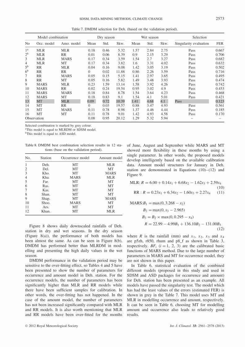
Figure 9. Amount model for January in Deh. station using MT model (x1 = p5zh, x2 = r850, x3 = rhum and x4 = p8_f).



Table 6. Number of parameters for amount model in Deh. station.

Model Jan. Feb. Mar. Apr. May Jun. Jul. Aug. Sep. Oct. Nov. Dec.

MLR 5 5 5 5 5 5 5 5 5 5 5 5RR 4 4 4 4 4 4 4 4 4 4 4 4MARS 9 4 6 14 1 1 1 1 1 1 1 11MT 20 17 23 6 1 1 1 1 1 1 4 3No. of Calibration data 72 78 86 39 11 2 9 4 6 18 16 54

• Finally, the model with the least-FER value is selectedas the best one.

In this study, no transformation has been used aspreprocessing for application of DMDM, MLRDM andSDSM. In the next section, modelling results and theadvantages and disadvantages of the proposed methodol-ogy are described.

3.4. Issue of parsimony

As mentioned in the previous sections of the paper, theproposed methodology consists of two distinct modules.Both in occurrence and amount simulations, number ofobservations versus number of model parameters are oneof the most important factors when comparing results ofdifferent models. Both MLR and RR methods use fixednumber of parameters for a specific number of predictors.But in DM methods, the number of parameters dependson the dataset structure and can be different for the samenumber of predictors. In this study, in order to addressissue of parsimony, Akaike information criterion (AIC)has been used. The AIC is a measure of goodness of fitinvolving not only the weighted errors, but the numberof observations, n , and the number of model parameters,p (Tong, 1983, p. 135):

AIC = n × ln

(Rm

n

)+ 2 × p (9)

The smaller the AIC, the better is the fit. Rm isloss function. It should be noted that, in the literature,different loss functions have been used for estimatingAIC. Examples can be found in Ljung (1999) and Olea(2006). In this study, FER (Equation (8)) is considered asloss function in Equation 10. In the next section, resultsand discussion of results are presented.

4. Results and discussion

As mentioned earlier, since the proposed occurrence andamount models are linear, stepwise regression has beenadopted to select the best combination of predictors.SDSM package uses the same predictors for occurrenceand amount of precipitation, but in this study, separatesets of predictors have been considered for modellingoccurrence and amount of precipitation. For example,the differences between provided degree of freedom inusing different dataset for occurrence and amount simu-lation have been presented in Figure 4 in Deh. station.

As shown in this figure, the results of MLRDM (possibil-ity of using different datasets for occurrence and amountmodelling), both in the calibration and validation periodsis slightly better than SDSM (same datasets for occur-rence and amount modelling). MLRDM performance hasbeen slightly better in producing monthly mean, standarddeviation and skewness both in the calibration and vali-dation periods. Also, q–q plots of observed versus com-puted precipitation have confirmed the better consistencyof MLRDM results distribution with the observed recordsparticularly in extreme values of the calibration period.But in validation period, this superiority is not significant.It should be noted that same comparison for all 12 stationshas been carried out and the results have shown minorimprovements of SDSM results when separate sets ofpredictors are used for occurrence and amount modelling.

Although the improvement of SDSM results canbe considered minor, since the procedure of predictorselection is automated in MLRDM, it can be consideredas a more reliable downscaling tool compared withSDSM. In the rest of this section, MLRDM results referto the results of the modified SDSM model which isreproduced in DMDM package, so that it can workwith different sets of predictors for occurrence andamount.

Tables 2 and 3 show the selected predictors for occur-rence and amount models in Deh., Kas. and Khan. sta-tions. In these tables, coefficients of determination forthe selected predictands and predictors have been pre-sented. It should be noted that all listed predictors aresignificant at p < 0.001. Selected predictors are mostlyrelative humidity and zonal velocity in different geopo-tential heights without any time lags. Generally, they arescattered in all of the nine boxes shown in Figure 1.

In the current research, 100 ensembles of precipitationhave been produced in each station. The mean resultsof ensembles in the three selected stations, namely Deh.,Kas. and Khan., are shown in Figures 5–7 for calibrationand validation periods.

Both MRLDM and DMDM performances havebeen acceptable in simulating the monthly mean forthe calibration and validation periods while for theselected three stations shown in Figures 5–7, DMDMdoes not show significant superiority over MLRDM.Figures 5–7 also show that the performance of DMDMhas been better than MLRDM in simulating the monthlystandard deviations. Skewness has been simulated betterby DMDM in the calibration and validation periodsas well.



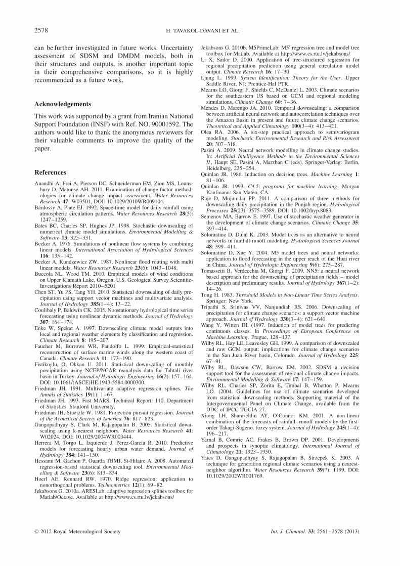
Table 7. DMDM selection for Deh. (based on the validation period).

Model combination Dry season Wet season Selection

No Occ. model Amo. model Mean Std. Skw. Mean Std. Skw. Singularity evaluation FER

1a MLR MLR 0.18 0.46 5.32 1.57 2.84 2.75 Pass 0.6672b MLR RR 0.01 0.06 8.39 0.9 2.15 3.29 Pass 0.7063 MLR MARS 0.17 0.34 3.59 1.54 2.7 3.27 Pass 0.6824 MLR MT 0.17 0.34 3.82 1.6 3.31 4.02 Pass 0.6325b RR MLR 0.04 0.16 9.08 1.42 3.05 3.19 Pass 0.5026b RR RR 0 0.02 11.88 0.86 2.26 3.59 Pass 0.7167 RR MARS 0.05 0.15 5.15 1.41 2.97 3.65 Pass 0.4958 RR MT 0.05 0.16 5.82 1.49 3.48 3.93 Pass 0.4749 MARS MLR 0.23 1.59 13.14 1.58 3.92 4.26 Pass 0.74210 MARS RR 0.02 0.24 19.54 0.95 3.02 4.9 Pass 0.45311 MARS MARS 0.18 0.84 8.78 1.54 3.64 4.23 Pass 0.46812 MARS MT 0.18 0.83 9.1 1.54 4.1 5.01 Pass 0.42113 MT MLR 0.09 0.72 10.39 1.41 4.68 4.1 Pass 0.12314 MT RR 0 0.03 19.57 0.88 3.47 4.93 Pass 0.56115 MT MARS 0.11 0.78 8.98 1.37 4.46 4.44 Pass 0.18516 MT MT 0.11 0.78 9.01 1.42 4.93 4.58 Pass 0.170Observation 0.08 0.95 20.12 1.29 5.32 5.94 – –

Selected combination is marked by grey colour.aThis model is equal to MLRDM or SDSM model.bThis model is equal to ASD model.

Table 8. DMDM best combination selection results in 12 sta-tions (base on the validation period).

No. Station Occurrence model Amount model

1 Deh. MT MLR2 Del. MT MT3 Kho. MT MARS4 Kha. MARS MLR5 Far. MT MT6 Ras. MT MT7 Kas. MT MT8 Shan. MT MT9 Shap. MT MARS10 Shoo. MARS MT11 Ars. MT MT12 Khan. MT MLR

Figure 8 shows daily downscaled rainfalls of Deh.station in dry and wet seasons. In the dry season(Figure 8(a)), the performance of both models hasbeen almost the same. As can be seen in Figure 8(b),DMDM has performed better than MLRDM in mod-elling and presenting the high daily values in the wetseason.

DMDM performance in the validation period may besensitive to the over-fitting effect, so Tables 4 and 5 havebeen presented to show the number of parameters foroccurrence and amount model in Deh. station. For theoccurrence models, the number of parameters has beensignificantly higher than MLR and RR models whilethere have been sufficient samples for calibration. Inother words, the over-fitting has not happened. In thecase of the amount model, the number of parametershas not been increased significantly compared with MLRand RR models. It is also worth mentioning that MLRand RR models have been over-fitted for the months

of June, August and September while MARS and MTshowed more flexibility in these months by using asingle parameter. In other words, the proposed modelsdevelop intelligently based on the available calibrationdata. Amount model structures for January in Deh.station are demonstrated in Equations (10)–(12) andFigure 9.

MLR: R = 6.00 + 0.14x1 + 6.68x2 − 1.62x3 + 2.59x4

(10)RR : R = 0.23x1 + 6.34x2 − 1.60x3 + 2.27x4 (11)

MARS:B1 = max(0, 3.268 − x2)

B2 = max(0, x3 − 2.965)

B3 = B2 × max(0, 0.295 − x4)

R = 22.99 − 4.99B1 + 136.10B2 − 131.00B3

(12)

where R is the rainfall (mm) and x1, x2, x3 and x4

are p5zh, r850, rhum and p8_f as shown in Table 3,respectively. BFi (i = 1, 2, 3) are the calibrated basicfunctions of MARS method. Due to the large number ofparameters in MARS and MT for occurrence model, theyare not shown in this paper.

In Table 6, statistical evaluation of the combineddifferent models (proposed in this study and used inSDSM and ASD packages for occurrence and amount)for Deh. station has been presented as an example. Allmodels have passed the singularity test. The model whichhas had the least values of the errors (estimated FER) isshown in grey in the Table 7. This model uses MT andMLR in modelling occurrence and amount, respectively.It can be seen in Table 6, choosing MT for modellingamount and occurrence also leads to relatively goodresults.



Tabl

e9.

Com

pari

son

ofM

LR

DM

and

DM

DM

perf

orm

ance

inal

lst

udie

dst

atio

n.

Cal

ibra

tion

Val

idat

ion

Dry

seas

onW

etse

ason

Dry

seas

onW

etse

ason

Stat

ion

Mod

elM

ean

Std.

Skw

.M

ean

Std.

Skw

.M

ean

Std.

Skw

.M

ean

Std.

Skw

.FE

RA

IC

Deh

.M

LR

DM

0.16

0.53

13.1

71.

472.

894.

040.

180.

465.

321.

572.

842.

750.

667

−22

653.

2D

MD

M0.

151.

2714

.33

1.46

4.83

4.74

0.09

0.72

10.3

91.

414.

684.

10.

123

−24

459.

1O

bs.

0.12

1.59

19.9

61.

476.

787.

760.

080.

9520

.12

1.29

5.32

5.94

——

Del

.M

LR

DM

0.33

0.69

6.21

2.18

4.04

4.31

0.33

0.64

3.6

2.3

4.04

3.11

0.30

9−2

322

1.7

DM

DM

0.26

1.46

11.0

42.

186.

826.

070.

170.

828.

492.

497.

325.

450.

038

−27

987.

1O

bs.

0.28

2.58

22.4

02.

128.

478.

200.

201.

489.

932.

338.

726.

23—

—K

ho.

ML

RD

M0.

250.

6313

.72.

624.

783.

460.

210.

495.

162.

784.

792.

730.

407

−21

349.

4D

MD

M0.

231.

5315

.03

2.55

7.79

7.25

0.15

1.01

11.6

52.

66.

93.

870.

069

−24

090.

4O

bs.

0.23

1.99

14.2

72.

559.

636.

770.

201.

5210

.84

2.08

9.28

8.45

——

Kha

.M

LR

DM

0.08

0.18

6.16

0.88

1.71

3.52

0.11

0.29

11.5

0.94

1.76

3.14

0.40

4−2

527

9.2

DM

DM

0.08

0.79

19.8

30.

862.

545.

370.

121.

0614

.08

0.97

2.48

4.38

0.05

8−2

693

4.2

Obs

.0.

071.

0224

.68

0.87

4.55

7.95

0.12

1.53

22.2

80.

763.

636.

39—

—Fa

r.M

LR

DM

2.68

5.35

4.04

3.7

5.31

2.32

2.6

5.78

3.8

3.89

5.85

2.55

0.17

2−3

180

1.2

DM

DM

2.66

7.72

5.12

3.75

7.78

3.56

2.18

7.83

5.61

3.71

8.29

3.72

0.05

6−3

207

9.8

Obs

.2.

699.

526.

293.

799.

644.

923.

1611

.47

6.77

3.78

10.2

04.

54—

—R

as.

ML

RD

M2.

915.

484.

094.

065.

932.

342.

996.

213.

994.

276.

522.

610.

038

−36

468.

7D

MD

M3.

058.

474.

784.

188.

463.

522.

798.

75.

034.

19.

544.

360.

012

−38

173.

0O

bs.

3.00

10.2

86.

624.

1610

.33

4.71

3.44

11.3

16.

063.

779.

384.

12—

—K

as.

ML

RD

M3.

044.

953.

332.

924.

142.

512.

815.

573.

692.

754.

322.

920.

219

−30

825.

6D

MD

M3.

058.

715.

893.

046.

353.

672.

47.

526

2.87

6.98

4.28

0.06

9−3

193

2.0

Obs

.3.

0211

.47

9.49

3.06

7.84

4.57

3.07

10.2

45.

842.

767.

154.

46—

—Sh

an.

ML

RD

M2.

814.

062.

92.

492.

871.

812.

644.

523.

092.

373.

122.

830.

140

−32

359.

4D

MD

M2.

867.

344.

952.

544.

713.

352.

345.

944.

242.

495.

574.

560.

042

−33

781.

1O

bs.

2.81

9.72

7.00

2.54

6.59

6.97

2.87

9.45

6.35

2.40

6.08

4.50

——

Shap

.M

LR

DM

0.07

0.47

20.2

1.5

3.36

3.57

0.07

0.37

12.3

11.

593.

493.

490.

424

−23

447.

2D

MD

M0.

070.

9923

.81.

574.

635

0.02

0.51

33.1

21.

715.

558.

270.

176

−24

561.

8O

bs.

0.07

1.20

24.9

01.

575.

875.

700.

030.

4918

.24

1.90

6.77

5.31

——

Shoo

.M

LR

DM

0.07

0.27

9.05

1.8

3.61

3.23

0.07

0.21

5.9

1.76

3.6

3.28

0.33

4−2

410

5.5

DM

DM

0.07

0.54

15.7

71.

834.

54.

290.

070.

4915

.91.

794.

34.

050.

065

−24

179.

2O

bs.

0.07

0.91

19.4

51.

836.

536.

590.

060.

7419

.86

2.24

7.53

5.01

——

Ars

.M

LR

DM

0.14

0.43

9.13

1.61

3.77

4.43

0.14

0.35

5.06

1.89

4.24

3.77

0.24

8−2

659

0.6

DM

DM

0.09

0.74

12.3

21.

625.

056.

380.

060.

459.

521.

946.

46.

270.

014

−36

906.

8O

bs.

0.09

1.19

23.6

51.

626.

106.

990.

050.

7123

.11

1.79

6.78

5.89

——

Kha

n.M

LR

DM

0.2

0.65

7.81

2.37

4.11

2.86

0.23

0.6

5.67

2.37

4.44

3.2

0.50

2−2

325

9.8

DM

DM

0.15

1.14

11.3

32.

45.

312.

610.

120.

9310

.21

2.37

5.59

2.89

0.07

1−2

710

1.9

Obs

.0.

151.

6116

.93

2.39

7.08

4.58

0.12

1.20

17.4

02.

487.

293.

81—

—



(a)

(b)

(c)

Figure 10. Five-year moving average for A2 and B2 scenarios in (a) Deh., (b) Kas. and (c) Khan. stations.

Table 8 presents DMDM best combinations in 12studied stations. According to this table, MT was themost selected model both for occurrence and amountmodelling. Then, MARS and MLR achieved the secondand third ranks, respectively. It is worthwhile to mentionthat in Kas. station best combination, according to FERcriteria, is MT-MARS (MT for occurrence and MARSfor amount modelling). But this combination producessingular rainfall values more than the threshold defined.So, based on singularity analysis MT-MT has beenreported as the best combination in this table.

Overall, the results have shown that MT can providea useful diagnostic tool for identifying the key determi-nants of precipitation amount at a given site, includingthreshold states in the atmosphere, or combinations ofconditions that generate extreme events.

Table 9 shows the comparison between MLRDMand DMDM performances in all studied station usingthe evaluation procedure in Equation (3). In this table,mean values, standard deviation (std.), skewness (skw.)

of the simulated and observed rainfall for dry and wetseasons for both calibration and validation datasetsare presented. FER and AIC values for comparing theresults of DMDM and MLRDM are shown in this tablefor the validation period as well. Both FER and AICvalues have been shown in this table show superiorityof DMDM over MLRDM.

To evaluate the climate change impacts on the studiedstations, SRES A2 and B2 scenarios have been consid-ered for the 2000–2050 period. In Figure 10, 5-yearmoving average of precipitation is presented for A2 andB2 scenarios in Deh., Kas. and Khan. stations. The resultsof downscaling using MLRDM and DMDM are gen-erally different because of the different values of biascorrection and VIF factors calculated in the calibrationperiod by these models. As it can be seen in Figure 10,except for Khan. station, the proposed models producedsignificantly different results compared with MLRDMmodel which shows high level of uncertainty associated



5th Percentile (MLRDM)

95th Percentile(MLRDM)

5th Percentile (DMDM)


Maximum (Calibration period)

Minimum (Calibration period)







0

500

1000

1500

2000

2000 2005 2010 2015 2020 2025 2030 2035 2040 2045 2050

Pre

cipi

tati

on (m

m)

Year

0.0

500.0

1000.0

1500.0

2000.0

2500.0

2000 2005 2010 2015 2020 2025 2030 2035 2040 2045 2050

Pre

cipi

tati

on (m

m)

Year







0.00

500.00

1000.0

1500.0

2000.0

2500.0

3000.0

2000 2005 2010 2015 2020 2025 2030 2035 2040 2045 2050

Pre

cipi

tati

on (m

m)

Year

(a)

(b)

(c)

Figure 11. Annual precipitation for A2 and B2 scenarios and [5, 95]th ensemble percentiles for DMDM and MLRDM in Deh., Kas. and Khan.Stations. (a) Deh. station (A2), (b) Deh. station (B2), (c) Kas. station (A2), (d) Kas. station (B2), (e) Khan. station (A2) and (f) Khan. station

(B2).

with downscaling modelling procedure in future climatechange projections.

To assess output uncertainty of the downscaled sce-narios using DMDM and MLRDM, annual precipitationof 5th and 95th percentiles of ensemble results for theboth scenarios in Deh., Kas. and Khan. stations and theirminimum and maximum in their calibration periods arepresented. As it can be seen in this Figure 11, the uncer-tainty bound of DMDM results is narrower than SDSMwhich shows less difficulty for the decision makers.

5. Conclusions

Presented results in this paper depict better performanceof the proposed model in preserving historical monthly

mean precipitation and closer estimation of historicalmonthly mean standard deviation and skewness comparedwith SDSM and ASD. Stepwise regression based onquantile evaluation is used here for meteorological feature(input) selection. DMDM has proved to be a suitablealternative for daily precipitation downscaling and itcan be also further developed for downscaling of otherconditional and unconditional meteorological variables.

Two proposed statistical norms, FER and AIC, havebeen efficiently used to evaluate the performances ofthe proposed downscaling models. Using FER and AICallows modeller to perform evaluations just based onmodel errors with and without incorporating issue ofparsimony.

Results of precipitation downscaling in 12 rain gaugestations scattered over three different basins in Iran









0.0

500.0

1000.0

1500.0

2000.0

2500.0

3000.0

2000 2005 2010 2015 2020 2025 2030 2035 2040 2045 2050

Pre

cipi

tati

on (m

m)

Year


95th Percentile(MLRDM)







5th Percentile(DMDM)




0.00

400.00

800.00

1200.0

1600.0

2000.0

2000 2005 2010 2015 2020 2025 2030 2035 2040 2045 2050

Pre

cipi

tati

on (m

m)

Year

0.0

200.0

400.0

600.0

800.0

1000.0

1200.0

1400.0

1600.0

1800.0

2000.0

2000 2005 2010 2015 2020 2025 2030 2035 2040 2045 2050

Pre

cipi

tati

on (m

m)

Year

(d)

(e)

(f)

Figure 11. Continued.

have shown that MT has been selected 11 and 8 times(from 12 models) for occurrence and amount modelling,respectively. While the total number of MT parametersis higher than SDSM and ASD, no over-fitting hasoccurred. On basis of the FER values estimated inthis study, DMDM has outperformed MLRDM in thenorthern basins with wet climate (Sefidrood and Mordab-anzali). The improvement in the performance of DMDMcompared with MLRDM in the semi-arid basins in thecase study of this research has not been as significantas its performance in the aforementioned wet basins. Itshould be noted that both DMDM and SDSM can be usedfor semi-arid/data sparse regions while application ofSDSM might be limited to seasonal or annual time scalesbecause of possibility of over fitting or ill-conditionoccurrence.

Analysis of daily time series of downscaled precipita-tion values in the 12 rain gauge stations used in the case

study of this research shows that except for Del. andKhan. stations, the differences between the results ofDMDM and MLRDM have been higher than the differ-ences between the values estimated for A2 and B2 scenar-ios by these models. This finding shows high uncertaintyassociated with downscaling techniques utilized in theclimate change related studies. While the need forcareful selection of proper climate change scenarios hasbeen emphasized in the previous studies, the resultsof this study have shown that uncertainty associatedwith downscaling technique is at least as important asscenario itself. Future work might consider the SDSMplatform coupled with nonlinear methods such as SVM,adaptive neuro-fuzzy inference systems (ANFIS) both inregression (=amount) and classification (=occurrence)mode. It must be noted that feature selection in this typeof modelling must be based on nonlinear evaluation,because a linear correlation is not valid. This issue



can be further investigated in future works. Uncertaintyassessment of SDSM and DMDM models, both intheir structures and outputs, is another important topicin their comprehensive comparisons, so it is highlyrecommended as a future work.

Acknowledgements

This work was supported by a grant from Iranian NationalSupport Foundation (INSF) with Ref. NO. 90001592. Theauthors would like to thank the anonymous reviewers fortheir valuable comments to improve the quality of thepaper.

References

Anandhi A, Frei A, Pierson DC, Schneiderman EM, Zion MS, Louns-bury D, Matonse AH. 2011. Examination of change factor method-ologies for climate change impact assessment. Water ResourcesResearch 47: W03501, DOI: 10.1029/2010WR009104.

Bardossy A, Plate EJ. 1992. Space-time model for daily rainfall usingatmospheric circulation patterns. Water Resources Research 28(5):1247–1259.

Bates BC, Charles SP, Hughes JP. 1998. Stochastic downscaling ofnumerical climate model simulations. Environmental Modelling &Software 13: 325–331.

Becker A. 1976. Simulations of nonlinear flow systems by combininglinear models. International Association of Hydrological Sciences116: 135–142.

Becker A, Kundzewicz ZW. 1987. Nonlinear flood routing with multilinear models. Water Resources Research 23(6): 1043–1048.

Buccola NL, Wood TM. 2010. Empirical models of wind conditionson Upper Klamath Lake, Oregon. U.S. Geological Survey Scientific-Investigations Report 2010–5201

Chen ST, Yu PS, Tang YH. 2010. Statistical downscaling of daily pre-cipitation using support vector machines and multivariate analysis.Journal of Hydrology 385(1–4): 13–22.

Coulibaly P, Baldwin CK. 2005. Nonstationary hydrological time seriesforecasting using nonlinear dynamic methods. Journal of Hydrology307: 164–174.

Enke W, Spekat A. 1997. Downscaling climate model outputs intolocal and regional weather elements by classification and regression.Climate Research 8: 195–207.

Faucher M, Burrows WR, Pandolfo L. 1999. Empirical-statisticalreconstruction of surface marine winds along the western coast ofCanada. Climate Research 11: 173–190.

Fistikoglu, O, Okkan U. 2011. Statistical downscaling of monthlyprecipitation using NCEP/NCAR reanalysis data for Tahtali riverbasin in Turkey. Journal of Hydrologic Engineering 16(2): 157–164.DOI: 10.1061/(ASCE)HE.1943-5584.0000300.

Friedman JH. 1991. Multivariate adaptive regression splines. TheAnnals of Statistics 19(1): 1–67.

Friedman JH. 1993. Fast MARS. Technical Report: 110, Departmentof Statistics. Stanford University,

Friedman JH, Stuetzle W. 1981. Projection pursuit regression. Journalof the Acoustical Society of America 76: 817–823.

Gangopadhyay S, Clark M, Rajagopalan B. 2005. Statistical down-scaling using k-nearest neighbors. Water Resources Research 41:W02024, DOI: 10.1029/2004WR003444.

Herrera M, Torgo L, Izquierdo J, Perez-Garcia R. 2010. Predictivemodels for forecasting hourly urban water demand. Journal ofHydrology 384: 141–150.

Hessami M, Gachon P, Ouarda TBMJ, St-Hilaire A. 2008. Automatedregression-based statistical downscaling tool. Environmental Mod-elling & Software 23(6): 813–834.

Hoerl AE, Kennard RW. 1970. Ridge regression: application tononorthogonal problems. Technometrics 12(1): 69–82.

Jekabsons G. 2010a. ARESLab: adaptive regression splines toolbox forMatlab/Octave. Available at http://www.cs.rtu.lv/jekabsons/

Jekabsons G. 2010b. M5PrimeLab: M5′ regression tree and model treetoolbox for Matlab. Available at http://www.cs.rtu.lv/jekabsons/

Li X, Sailor D. 2000. Application of tree-structured regression forregional precipitation prediction using general circulation modeloutput. Climate Research 16: 17–30.

Ljung L. 1999. System Identification: Theory for the User . UpperSaddle River, NJ: Prentice-Hal PTR.

Mearns LO, Giorgi F, Shields C, McDaniel L. 2003. Climate scenariosfor the southeastern US based on GCM and regional modelingsimulations. Climatic Change 60: 7–36.

Mendes D, Marengo JA. 2010. Temporal downscaling: a comparisonbetween artificial neural network and autocorrelation techniques overthe Amazon Basin in present and future climate change scenarios.Theoretical and Applied Climatology 100(3–4): 413–421.

Olea RA. 2006. A six-step practical approach to semivariogrammodeling. Stochastic Environmental Research and Risk Assessment20: 307–318.

Pasini A. 2009. Neural network modelling in climate change studies.In: Artificial Intelligence Methods in the Environmental SciencesII , Haupt SE, Pasini A, Marzban C (eds). Springer-Verlag: Berlin,Heidelberg, 235–254.

Quinlan JR. 1986. Induction on decision trees. Machine Learning 1:81–106.

Quinlan JR. 1993. C4.5: programs for machine learning . MorganKaufmann: San Mateo, CA.

Raje D, Mujumdar PP. 2011. A comparison of three methods fordownscaling daily precipitation in the Punjab region. HydrologicalProcesses 25(23): 3575–3589. DOI: 10.1002/hyp.8083.

Semenov MA, Barrow E. 1997. Use of stochastic weather generator inthe development of climate change scenarios. Climatic Change 35:397–414.

Solomatine D, Dulal K. 2003. Model trees as an alternative to neuralnetworks in rainfall-runoff modeling. Hydrological Sciences Journal48: 399–411.

Solomatine D, Xue Y. 2004. M5 model trees and neural networks:application to flood forecasting in the upper reach of the Huai riverin China. Journal of Hydrologic Engineering 9(6): 275–287.

Tomassetti B, Verdecchia M, Giorgi F. 2009. NN5: a neural networkbased approach for the downscaling of precipitation fields – modeldescription and preliminary results. Journal of Hydrology 367(1–2):14–26.

Tong H. 1983. Threshold Models in Non-Linear Time Series Analysis .Springer: New York.

Tripathi S, Srinivas VV, Nanjundiah RS. 2006. Downscaling ofprecipitation for climate change scenarios: a support vector machineapproach. Journal of Hydrology 330(3–4): 621–640.

Wang Y, Witten IH. (1997. Induction of model trees for predictingcontinuous classes. In Proceedings of European Conference onMachine Learning . Prague, 128–137.

Wilby RL, Hay LE, Leavesley GH. 1999. A comparison of downscaledand raw GCM output: implications for climate change scenariosin the San Juan River basin, Colorado. Journal of Hydrology 225:67–91.

Wilby RL, Dawson CW, Barrow EM. 2002. SDSM–a decisionsupport tool for the assessment of regional climate change impacts.Environmental Modelling & Software 17: 147–159.

Wilby RL, Charles SP, Zorita E, Timbal B, Whetton P, MearnsLO. (2004. Guidelines for use of climate scenarios developedfrom statistical downscaling methods. Supporting material of theIntergovernmental Panel on Climate Change, available from theDDC of IPCC TGCIA 27.

Xiong LH, Shamseldin AY, O’Connor KM. 2001. A non-linearcombination of the forecasts of rainfall–runoff models by the first-order Takagi-Sugeno. fuzzy system. Journal of Hydrology 245(1–4):196–217.

Yarnal B, Comrie AC, Frakes B, Brown DP. 2001. Developmentsand prospects in synoptic climatology. International Journal ofClimatology 21: 1923–1950.

Yates D, Gangopadhyay S, Rajagopalan B, Strzepek K. 2003. Atechnique for generation regional climate scenarios using a nearest-neighbor algorithm. Water Resources Research 39(7): 1199, DOI:10.1029/2002WR001769.


improved statistical downscaling of daily precipitation using sdsm platform and data-mining methods

Documents