importance of crustal corrections in the...

Importance of crustal corrections in the developmentof a new global model of radial anisotropy

M. P. Panning,1 V. Lekić,2,3 and B. A. Romanowicz2

Received 2 March 2010; revised 31 August 2010; accepted 20 September 2010; published 24 December 2010.

[1] Accurately inferring the radially anisotropic structure of the mantle using seismicwaveforms requires correcting for the effects of crustal structure on waveforms. Recentstudies have quantified the importance of accurate crustal corrections when mapping uppermantle structure using surface waves and overtones. Here, we explore the effects of crustalcorrections on the retrieval of deep mantle velocity and radial anisotropy structure. We applya new method of nonlinear crustal corrections to a three‐component surface and bodywaveform data set and invert for a suite of models of radially anisotropic shear velocity. Wethen compare the retrieved models against each other and a model derived from an identicaldata set but using a different nonlinear crustal correction scheme.While retrieval of isotropicstructure in the deep mantle appears to be robust with respect to changes in crustalcorrections, we find large differences in anisotropic structure that result from the use ofdifferent crustal corrections, particularly at transition zone and greater depths. Furthermore,anisotropic structure in the lower mantle, including the depth‐averaged signature in thecore‐mantle boundary region, appears to be quite sensitive to choices of crustal correction.Our new preferred model, SAW642ANb, shows improvement in data fit and reduction inapparent crustal artifacts. We argue that the accuracy of crustal corrections may currentlybe a limiting factor for improved resolution and agreement between models of mantleanisotropy.

Citation: Panning, M. P., V. Lekić, and B. A. Romanowicz (2010), Importance of crustal corrections in the developmentof a new global model of radial anisotropy, J. Geophys. Res., 115, B12325, doi:10.1029/2010JB007520.

1. Introduction

[2] Global seismic tomography shows excellent promisefor illuminating current mantle flow patterns. In particular,isotropic models have shown strong convergence in the long‐wavelength structure, and have been revealing finer and finerdetails in structure of isotropic S velocity [Mégnin andRomanowicz, 2000; Gu et al., 2003; Ritsema et al., 2004;Montelli et al., 2006; Houser et al., 2008; Simmons et al.,2009] as well as P velocity [Montelli et al., 2004; Li et al.,2006; Houser et al., 2008]. These provide an excellentconstraint on the current mantle thermal structure underthe assumption that lateral velocity perturbations can beexplained primarily as thermal variations. Using thisassumption, the models can then be related to mantle flow bydetermining the associated density perturbations due to thethermal structure. Some models [e.g., Simmons et al., 2009]attempt to incorporate other geodynamic data such as free‐air gravity data and dynamic topography to more directly

constrain the density field driving flow, but, in general, iso-tropic models allow for only an indirect connection withmantle flow patterns.[3] Models including anisotropic structure, however, have

the potential to more directly illuminate flow. This is becausedynamic processes in the mantle can produce seismicallyobservable anisotropy either through alignment of contrast-ing materials and melt (shape preferred orientation or SPO) orthe alignment of the crystallographic axes of intrinsicallyanisotropic minerals (lattice preferred orientation or LPO).Kinematic modeling of LPO [Kaminski and Ribe, 2001]produced through mantle flow models [e.g., Becker et al.,2008] suggest that upper mantle anisotropy can be wellmodeled using such an approach, but care must be taken ininterpreting the results as different LPO deformation modesare possible [Karato et al., 2008].[4] At this time, several global models of radial anisotropy,

where a vertical axis of symmetry is assumed, are available[Boschi and Dziewonski, 2000; Beghein and Trampert,2004a; Panning and Romanowicz, 2006; Kustowski et al.,2008], but as pointed out by Becker et al. [2008], significantdifferences remain between anisotropic models. In order toprovide robust constraints on geodynamic modeling, it is clearthat there needs to be some convergence between differentmodels to increase confidence in the resolved structures.[5] One potential source of errors and inconsistencies

between anisotropic models is through the use of crustalcorrections, which attempt to remove the signals that arise

1Department of Geological Sciences, University of Florida, Gainesville,Florida, USA.

2Berkeley Seismological Laboratory, University of California,Berkeley, California, USA.

3Now at Department of Geological Sciences, Brown University,Providence, Rhode Island, USA.

Copyright 2010 by the American Geophysical Union.0148‐0227/10/2010JB007520

JOURNAL OF GEOPHYSICAL RESEARCH, VOL. 115, B12325, doi:10.1029/2010JB007520, 2010

B12325 1 of 18

http://dx.doi.org/10.1029/2010JB007520

due to crustal structure from those originating in the mantle.As pointed out by Bozdağ and Trampert [2008], crustalcorrections have a different impact on Love and Rayleighwaves, and thus imperfect crustal corrections have thepotential to bias models of radial anisotropy in the uppermantle. These findings were confirmed by Lekić et al. [2010],who extended this analysis to the full waveforms of bothsurface waves and overtones. However, no quantitativeanalysis has yet been performed to investigate the effectof imperfect crustal corrections on a complete long‐periodwaveform data set including both body and surface waves,and the associated potential contamination of deep mantlestructure. This is one of the goals of our study.[6] Accurate crustal corrections are, however, nontrivial to

perform. One computationally inexpensive approach is tomodel the crustal effects as linear perturbations in topographyof the surface/seafloor and Mohorovičić discontinuity (orMoho) from a reference model, and this approach has beenused in the development of many tomographic models,including an earlier model developed from the same dataset applied here [Panning and Romanowicz, 2004]. How-ever, the crust clearly has very strong heterogeneity in boththickness and velocity structure and strongly deviates fromlinearity. Boschi and Ekström [2002] attempted to account forthis nonlinearity by calculating surface wave modes for theappropriate crustal structure at each point along the pathbetween source and receiver. Another approach to dealingwith this nonlinearity, proposed by Montagner and Jobert[1988], is to divide the Earth into a set of tectonic regions.Within each region, a different reference model is definedwhich can be used to calculate appropriate eigenfunctions forsurface waves or normal modes. These different regionalizedmodels can include crustal thicknesses and velocity structuresdifferent from the global reference model. This would thencapture most of the nonlinearity due to strong deviations froma single global reference model, while further deviationscould then be modeled linearly. This approach has theadditional benefit of allowing sensitivity to deeper velocitystructure to also be calculated using the suite of tectonicmodels, therefore capturing nonlinearity introduced in thatfashion as well. This approach was independently refined byMarone and Romanowicz [2007] andKustowski et al. [2007],and implemented in the creation of two recent anisotropicmodels [Panning and Romanowicz, 2006; Kustowski et al.,2008]. However, as pointed out earlier, there are still manydifferences between the anisotropic structure in these twomodels. Is there another way to better model crustal effects?Recently, Lekić et al. [2010] have proposed a more compu-tationally inexpensive way of capturing the nonlinear effectsof crustal structure. This method, like that proposed byMontagner and Jobert [1988], relies on first defining a suiteof tectonic regions. However, rather than using these modelsto define a new set of eigenfunctions, in this method wesimply invert for the appropriate perturbations to the crustalmodel that account for the nonlinearity for different subsets ofmodes (e.g., fundamental mode Love and Rayleigh wavesand overtones). When performing the actual inversion, weonly need to use the appropriate modified crustal model ratherthan tracking multiple crustal models and sets of eigen-functions. At first glance, it might appear that this simpli-fied approach may not capture the nonlinearity as well asthe Montagner and Jobert [1988] approach, but numerical

simulations suggest the method performs quite well [Lekićet al., 2010].[7] In this study, we quantify the contamination of deep

mantle velocity and anisotropic structure that can result fromdifferent ways of performing crustal corrections. Our workcomplements the analyses carried out previously by Bozdağand Trampert [2008] and Lekić et al. [2010] on surfacewaves and overtones, respectively. We do this by applyingdifferent implementations of the computationally efficient“modified linear corrections” (MLC) approach of Lekić et al.[2010] to develop a suite of global radially anisotropic modelsusing the same parameterization and data set as that used inthe development of the global model SAW642AN [Panningand Romanowicz, 2006]. By contrasting the retrievedvelocity and anisotropic structures between these models andSAW642AN, which was developed using a different non-linear crustal corrections technique based on theMarone andRomanowicz [2007] approach (hereafter referred to as NLC),we will demonstrate that crustal corrections can substantiallyaffect the retrieval of anisotropic structure in the deep mantle,even in the D″ region. Finally, we will present a preferredradially anisotropic mantle model, SAW642ANb, con-structed using MLC and capable of providing a better over-all fit to the data even with smaller overall model size,while removing some signatures in the isotropic portion ofSAW642AN that appear to be crustal artifacts.

2. Modeling Approach

[8] Themodels presented here are developed with the sameparameterization and waveform data set as used in thedevelopment of SAW642AN [Panning and Romanowicz,2006]. Additionally, the same basic theory, nonlinear asymp-totic coupling theory (NACT) [Li and Romanowicz, 1995], isused to model the waveforms as in that model.Wewill brieflydescribe this theory and the waveform data set here, but moredetailed explanations are given by Panning and Romanowicz[2006] and Li and Romanowicz [1995].

2.1. Waveform Data Set and Theory

[9] The waveform data used in this study consist of three‐component broadband surface waveforms (short‐periodcorner of 80 s and cutoff of 60 s) as well as body waveforms(short period corner of 40 s and cutoff of 32 s). The wave-forms are windowed to separate various energy wave packets(e.g., separating fundamental mode and overtone surfacewaves, as well as different body wave energy packets), whichenhances resolution of transition zone and lower mantlestructure [Mégnin and Romanowicz, 1999]. The final data setincludes over 120,000 wave packets with over 4 million datapoints (Table 1) [Panning and Romanowicz, 2006].[10] The waveforms and their sensitivity to aniso-

tropic velocity structure are modeled using NACT [Li andRomanowicz, 1995]. This theory is a normal mode basedperturbation approach that includes both along branch andcross‐branch coupling of modes in order to develop 2‐Dsensitivity kernels in the vertical plane defined by the greatcircle path between source and receiver. This theory bringsout the ray character of sensitivity while also includingsome of the off‐path sensitivity due to finite frequencyeffects. It also includes effects of multiple forward scattering[Romanowicz et al., 2008; Panning et al., 2009].

PANNING ET AL.: IMPORTANCE OF CRUSTAL CORRECTIONS B12325B12325

2 of 18

[11] As in SAW642AN, the model is parameterized interms of the Voigt average isotropic S velocity, VS, and theanisotropic parameter x, which can be written in terms of thehorizontally and vertically polarized S velocities (VSH andVSV, respectively) as

V 2S ¼ 2V 2

SV þ V 2SH

3ð1Þ

� ¼ V 2SH

V 2SV

: ð2Þ

We also assume the same scaling relationships for perturba-tions to P velocity and the other two anisotropic parametersas in the development of SAW642AN. While many mathe-matically equivalent parameterizations are possible, wechoose this one rather than one with separate VSH and VSV

models, for example, because it allows us to tune dampingspecifically on the anisotropic portion of the model. Withseparate inversions, where the anisotropy is proportionalto the difference between the two models, the uncertaintybecomes quite large, and it is difficult to constrain theanisotropy to be small in order to test whether anisotropy isreally required by the data.[12] Finally, the spatial parameterization of the model is the

same as SAW642AN, with 16 variably spaced cubic b splineswith depth [Mégnin and Romanowicz, 2000], and 642 equallyspaced spherical splines laterally [Wang and Dahlen, 1995].This provides a nominal lateral resolution of ∼800 km, andvariable depth resolution that is approximately scaled withdata coverage.

2.2. Improved Crustal Corrections

[13] The first anisotropic model developed with this dataset [Panning and Romanowicz, 2004, hereafter referred to asPR04] was developed with simple linear crustal corrections,although separate crustal models were used for the portions ofthe data primarily sensitive to VSH or VSV. In classical normalmode theory, the linear effect of crustal structure can bewritten

�!2k ¼ 2!k�!k ¼

X

d

r2dhd �; �ð ÞHdk �; �ð Þ; ð3Þ

where dwk is the eigenfrequency perturbation of the kthnormal mode, rd is the radius of the dth discontinuity in theglobal reference model, hd represents the perturbations intopography, and Hd is the calculated sensitivity to disconti-nuity topography.

[14] In the development of SAW642AN, we attempted toimprove the crustal corrections by implementing the here-after MR07 Marone and Romanowicz [2007] nonlinearcrustal corrections, an approach we will henceforth refer to asNLC. In this approach, we defined a suite of models for 5tectonic regions based on CRUST2.0 [Bassin et al., 2000],and calculated the appropriate eigenfunctions for each model.Each of these models differed from the global referencemodel in both thickness and velocity structure, with theregionalized models having a three‐layer velocity structuresimplified from CRUST2.0. At each point along the pathbetween source and receiver we then calculated a crustalcorrection term that had a nonlinear portion due to the dif-ference in eigenfrequency between the tectonic model andPREM, as well as further linear corrections for the deviationfrom the regionalized model. Additionally, we used sensi-tivity kernels calculated from the appropriate regionalizedeigenfunctions. We can summarize this approach as treatingthe perturbation of a mode k from a global reference model(GRM) as the sum of a linear perturbation from a local ref-erence model (LRM) plus the difference between the eigen-frequency of the mode in the GRM and the LRM, e.g.,

2!k�!k ¼X

d

rLRMd

� �2hLRMd �; �ð ÞHd;LRM

k �; �ð Þ þ !LRMk � !

GRMð Þk ;

ð4Þ

where wkLRM and wk

GRM are the eigenfrequencies in the localand global reference models, respectively, and the sensitivityis now explicitly calculated in the local reference model (seeequations (1) and (2) of MR07).[15] The NLC approach is fairly computationally intensive,

primarily due to the input/output requirements necessaryto track eigenfunctions and kernels for multiple models. Inorder to ideally obtain a similar level of approximation to thenonlinear problem of crustal corrections with a less com-putationally intensive approach, Lekić et al. [2010] haverecently proposed an alternative approach of modified linearcorrections (MLC). We start by rewriting the standard wayof expressing linear crustal corrections due to topography ofthe surface and Moho (equation (3)) in a matrix form as

w ¼ H�r; ð5Þ

wherew is a column vector of lengthN (the number of modesconsidered) with the kth element defined by 2wkdwk, theeigenfrequency perturbation to the kth mode, H is a 2 × Nmatrix summarizing the sensitivity to topography of the twoboundaries (e.g., elements can be written as rd

2Hkd), and dr is

the perturbation of the two boundaries. In the NLC approach,we divide w into two terms (a nonlinear and a linear one),where the linear one is defined by making the appropriatechanges to H for the different tectonic models. In the newMLC approach, we choose to instead represent the nonline-arity by adding in a term to the topography perturbations,writing instead

w ¼ H �rþ cmdð Þ; ð6Þ

where the subscripts m and d indicate that we invertfor different correction factors for different mode types m(separating out spheroidal and toroidal modes, as well as

Table 1. Percent Variance Reduction for Data Subsetsa

Data Set SAW642AN Model A Model B Model C Model D

Fundamental 60.8 61.8 61.9 62.0 61.7Overtones 48.7 51.8 52.1 52.7 52.1Total surface wave 56.2 57.9 58.1 58.4 58.0Body waves 44.8 46.5 47.9 49.1 45.4Total 52.1 53.8 54.5 55.1 53.5

aNote that all variance reduction numbers are calculated with the crustalcorrections used in their development (NLC for SAW642AN, MLC formodels A–C, MLC for model D surface waves, and NLC for model D bodywaves).


3 of 18

fundamental and overtone modes), and different discon-tinuities d (Moho and surface topography). The inversion isdone to minimize the difference between eigenfrequenciescalculated with this correction compared to those calculateddirectly from each tectonic model (which once again includesdifferences from the global model in both crustal thicknessand velocity structure). Unlike the NLC approach, once thecorrection factors are precalculated, there is no additionalcomputational cost when inverting as compared to linearcorrections, which makes using larger numbers of crustalmodels more practical. In this study, we utilize 7 differenttectonic regions [as defined by Lekić et al. [2010] based onCRUST2.0 and only consider corrections to the Mohotopography. Even larger numbers of regions could be utilizedto more accurately reflect the crust with only a relativelysmall increase in time necessary to precompute the correctionfactors, but no increase in the computational costs of theactual inversion. As a drawback, however, we lose the abilityin this method to define kernels using eigenfunctions in theregionalized models. Additionally, there is an implicitassumption that only self‐coupling is important, which maybe adequate for fundamental modes (although couplingbetween fundamental Love and Rayleigh modes has beenshown to be important in the presence of anisotropy [e.g.,Park, 1993; Beghein et al., 2008]), but is even more prob-lematic for surface wave overtones, and generally not ade-quate to describe body wave sensitivity. While there aretherefore some trade‐offs between the methods in terms ofthe modeling of the nonlinearity, Lekić et al. [2010] showedsignificant improvement over standard linear corrections,based on numerical testing.

3. Results

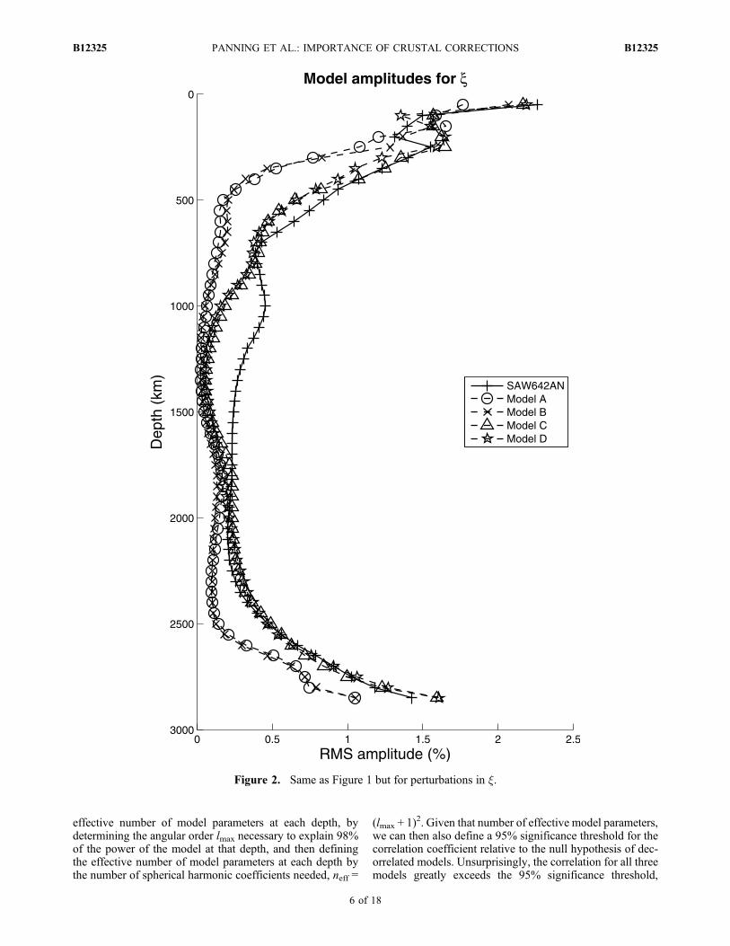
[16] We applied this new MLC approach to crustal cor-rections and performed 4 additional model inversion itera-tions starting from SAW642AN. Three classes of modelswere created, based upon the corrections used for the bodywave portion of the data set. As discussed in section 2.2, thesecrustal corrections are derived separately for fundamental andovertone surface waves. However, no explicit correctionfor body waves is developed, as the method implicitly onlyincludes self‐coupling, which is not correct for body wavesensitivity. With that in mind, we attempted to do the inver-sion with three different approaches for the body wave cor-rections: (1) linear corrections only from CRUST2.0, (2) thecorrections derived for the overtone modes, or (3) the NLCcorrections used in the development of SAW642AN. Forthe rest of the paper, wewill be referring to four models (A, B,C, and D). Model A includes only the linear corrections forbody wave packets (while still utilizing MLC corrections forthe fundamental mode and overtone surface waves), while Band C use the overtone‐derived corrections for the bodywaves. Model D was derived using the NLC corrections forthe body wave data. Damping for all 4 models was chosen inorder to produce a similar model size for the isotropic portionof the model as in SAW642AN, as defined by the root meansquared amplitude as a function of depth (Figure 1). Thedamping for the anisotropic portion of models A and B waschosen so as to strongly reduce the amplitude of anisotropyat transition zone and greater depths (Figure 2), for reasons

to be discussed later, while models C and D have similaranisotropic amplitudes to SAW642AN.[17] The variance reduction numbers for models A, B, C,

and D as discussed above, as well as SAW642AN are sum-marized in Table 1. All four models are able to achievesuperior variance reduction as compared to SAW642ANwiththe NLC crustal corrections for the entire data set. Model B isable to achieve slightly better fit than model A with similarmodel size, which suggests that applying the overtone basedcorrection to the body waves provides an improvement oversimple linear corrections. Model C shows slightly better datafit, although with a more strongly anisotropic model, whichmeans there were more effective model parameters. Despite asimilar model size to model C, model D has the worse data fitof the four new models, suggesting that in this case, the NLCcorrections for the body wave data do not show improvementrelative to the MLC corrections. However, all of the changesin fit between the models discussed here are small anddependent on the damping choices made in the inversion, andso it is difficult to make a statistical argument for one modelover another. A simple application of the F test with degreesof freedom defined as n−p, where n is the number of wavepackets in the inversion and p the number of model param-eters, would suggest that an estimated variance ratio as smallas 1.01 (corresponding to an overall variance reductionof >52.7%) would be significantly improved fit overSAW642AN at the 95% confidence level, meaning that allfour models have statistically significant improved fit relativeto SAW642AN. However, such a test is questionable in thissituation where assumptions of data independence are likelyviolated, and so this can only be treated as a lower bound ofthe real confidence threshold. For example, reducing thenumber of degrees of freedom by a factor of 10 (as an esti-mated upper bound) increases the required variance reductionthreshold for 95% confidence to 55.8%, which would meanthat models A–D are just short of a statistically significantimprovement in fit over SAW642AN. Regardless, it is clearthat the differences between each of these models as well asrelative to SAW642AN are small, but quite close to a 95%confidence threshold.

3.1. Isotropic VS Structure

[18] The isotropic VS structure is quite similar toSAW642AN, as well as other global shear velocity models(shown for model B in Figure 3). As usual we see tectonicstructure at shallow depths with strong difference in oceanicand continental velocities, and a general trend of increasingvelocity as a function of age in the oceanic regions. As wemove down into the transition zone, the strongest anomaliesare associated with regions of subduction, while the ampli-tude of structure becomes much smaller through midmantledepth ranges. Finally, we see a degree 2 pattern in the core‐mantle boundary region, with a fast ring around the two largelow‐velocity provinces often called the superplumes.[19] In order to quantify differences between models, we

also calculated the correlation of the isotropic portions ofmodels A, B, C, and D to SAW642AN as a function of depth(Figure 4). These correlations are calculated by expanding themodels in spherical harmonics to degree 24 at each depth, andthen calculating the correlation across those spherical har-monic coefficients. This approach also allows us to define an


4 of 18

Figure 1. Root‐mean‐square amplitude (in percent perturbation) for the isotropic VS portion ofSAW642AN (black solid line), as well as models A, B, C, and D as discussed in the text (with symbolsdefined in legend).


5 of 18

effective number of model parameters at each depth, bydetermining the angular order lmax necessary to explain 98%of the power of the model at that depth, and then definingthe effective number of model parameters at each depth bythe number of spherical harmonic coefficients needed, neff =

(lmax + 1)2. Given that number of effective model parameters,we can then also define a 95% significance threshold for thecorrelation coefficient relative to the null hypothesis of dec-orrelated models. Unsurprisingly, the correlation for all threemodels greatly exceeds the 95% significance threshold,

Figure 2. Same as Figure 1 but for perturbations in x.


6 of 18

although there are larger changes in structure in the transi-tion zone and the upper portion of the lower mantle (∼400–1500 km) as compared to the uppermost and lowermostmantle. Since the structure at these depth ranges where we areseeing differences is primarily controlled by the body wavedata, it is unsurprising that model D, which uses the samecrustal corrections for body waves as in the development ofSAW642AN, remains highly correlated in all depth ranges.It should be noted here that the F test used to determinethe 95% confidence level assumes independent realizationsof the models, while models A–D are all the products ofdamped nonlinear inversions starting from SAW642AN,which would indicate that the models are not entirely inde-pendent from SAW642AN and therefore should require alarger correlation coefficient for 95% confidence. However,4 iterations were performed from the starting model, withdamping at each step penalizing large values relative tothe reference model PREM rather than the starting model,

and therefore the assumption of independence should bereasonable.[20] While the changes in these transition zone and mid-

mantle depth ranges are not particularly apparent whencomparing maps on global scales, such as in Figure 3, thedifferences become more clear when comparing the radialcorrelation functions of the different models (Figure 5).Radial correlation functions plot the correlation coefficientbetween different depths of the same model. In SAW642AN,there is a fairly strong anticorrelation between the shallowtectonically dominated structure and the structure of thetransition zone and the uppermost lower mantle between600 and 1000 km. Additionally, we see a strong positivecorrelation develop between the uppermost mantle andthe midmantle depths between 1000 and 2000 km depth.While it is possible that such structure could reflect the realvelocity structure of the Earth, it is not generally presentin other global models of shear velocity structure such as

Figure 3. Perturbations in VS plotted for several depths in the mantle for model B discussed in the text. Allslices use the same color scale defined in color bar. Values are perturbations in percent from the velocity ofthe reference model PREM.


7 of 18

Figure 4. Correlation coefficient of the VSmodels A, B, C, and D (dashed lines with symbols as defined inthe legend) to SAW642AN as a function of depth up to spherical harmonic degree 24. The solid black linewith pluses shows the 95% confidence threshold for significant correlation, calculated as described in thetext.


8 of 18

S362WMANI [Kustowski et al., 2008] (Figure 5). This sig-nature is strongly reduced in models A–C, as shown inFigure 5, strongly suggesting that the MLC approach hasreduced the effect of crustal artifacts. Model D, on the otherhand, retains this signature (although with some reductionof the corresponding anticorrelation between transition zonestructure and the deeper structure), suggesting that the crustalcorrections for the body waves are the important controllingfactor for this feature. Of course, there is still evidence for

much more structure in the radial correlation functions forall models discussed here than for S362WMANI, but this isprimarily due to the larger degree of smoothing present inthat model.

3.2. Anisotropic Structure

[21] While the isotropic portion of the structure remainedrelatively robust regardless of crustal correction used, withthe exception of the apparent removal of some artifacts in the

Figure 5. Radial correlation functions for isotropic VS for SAW642AN, S362WMANI [Kustowski et al.,2008] and models A, B, C, and D. Radial correlation functions graphically display the correlation betweenthe structure in a model at different depths as represented by the values on the x and y axes.


9 of 18

transition zone and upper part of the lower mantle, thechanges are more pronounced in the anisotropic portion of themodel (Figure 6).[22] In the upper mantle, the correlations remain relatively

high, generally ranging between 0.7 and 0.8 for models A, B,

and C, and slightly higher for model D. In general, the signalsin SAW642AN discussed by Panning and Romanowicz[2006] remain (Figure 7). We still image the positive x per-turbation (i.e., VSH increased relative to VSV) beneath oceansat shallow depths that slowly decreases down to 300 km

Figure 6. Same as Figure 4 but for the x parameter.


10 of 18

depth, as well as the positive x perturbation beneath cratonicregions which is prominent between 200 and 300 km. Thesesignatures remain consistent with the interpretation offocused deformation in the asthenosphere [Gung et al., 2003].We also still image the positive x perturbations beneathspreading centers between 150 and 200 km depth, which maybe interpreted as a signal of vertical ridge feeding flow. Thesesignatures appear to be robust to the different crustal cor-rections, and therefore we can continue to use them to makemeaningful geodynamic inferences.[23] The correlations are much lower in the transition zone

and lower mantle. Model A, in particular, is less significantlycorrelated to SAW642AN throughout most of the lowermantle. Models B and C also have relatively low values ofcorrelation throughout most of the lower mantle, generallyranging between 0.4 and 0.65, but all models are correlatedwith SAW642AN above the 95% confidence thresholdexcept for a small range between 2000 and 2500 km depth,although we should once again note the caveat aboutthe correlation significance thresholds, as discussed insection 3.1. Once again, model D, which has the samecrustal corrections for body waves as SAW642AN, has verysimilar structure to SAW642AN throughout the transitionzone and lower mantle.[24] It is also interesting to look at the upper mantle radial

correlation functions for x in the new models and comparethem with SAW642AN and S362WMANI (Figure 8).Bozdağ and Trampert [2008] point out in their inversions

that the spurious anisotropic structure due to inadequatecrustal correction has a pronounced sign change between 50and 150 km depth. The radial correlation functions showevidence of a sign change near 200 km depth (indicated by asmall anticorrelation between structure above and below thatdepth) in SAW642AN andmodel A, as well as a possible signchange near 150 km depth in S362WMANI. Model Dappears to show such a sign change a little deeper, near300 km depth. No such sign change is apparent in models Bor C. While there is no strong evidence to indicate that such asign change does not reflect real Earth structure, it is anothersuggestion that model B shows less evidence of crustalartifacts than previous models. Ideally, we could attempt toquantitatively evaluate trade‐offs between shallow structureand deeper structure in the different models to determinemore accurately whether the observed anticorrelations aretruly artifacts. One possible approach to this is to evaluatetrade‐offs using the resolution matrix, and see if such trade‐offs are, for example, more pronounced for model A or Dthan for B or C. We attempted this (see auxiliary material),but the results simply demonstrated that there was little dif-ference in the resolution matrices of the models.1 Of coursetrade‐off analysis using the resolution matrices for the dif-ferent inversions only shows the differences due to problemgeometry (which is identical for all cases), damping (which

Figure 7. Perturbations in x relative to PREM (in percent) plotted for model B for several depths in theupper mantle.

1Auxiliary materials are available in the HTML. doi:10.1029/2010JB007520.


11 of 18

does differ, although not by large margins) and theory usedto calculate sensitivity (which is the same for models A–Cbut differs for SAW642AN and model D due to the use ofkernels calculated in the regionalized models rather thanPREM). It does not, however, directly address trade‐offs thatmay appear due to real data not being adequately modeled bythe particular choice of theory, such as the different approachto crustal corrections used here. These different theoreticalapproaches clearly cause significant changes to the resultingmodels although the resulting resolution matrices are all quite

similar. Ideally, one could better address this issue byperforming a test where the data set is recalculated using fullynumerical synthetics and a known crustal model, howeverthis is in many ways similar to the work done by Bozdağ andTrampert [2008] and Lekić et al. [2010], and beyond thescope of this study. Therefore, we cannot definitively con-clude that the anticorrelation is indeed an artifact, but giventhe results of Bozdağ and Trampert [2008], it is cause forconcern.

Figure 8. Upper mantle and transition zone radial correlation functions for x for SAW642AN,S362WMANI, and models A, B, C, and D.


12 of 18

[25] Because model B fits the data better than model A(with the caveats about statistical significance discussed insection 3), and reduces possible crustal artifacts, it appearsthat the use of overtone‐based corrections to the body wavedata produces a better model than using only linear correc-tions for the body wave portion of the data set, or using theNLC corrections used in the development of SAW642AN.While model B is our preferred model, all four models Athrough D will be made available through the first author’sWeb site.[26] Because of the general decrease in correlation of

anisotropic structure beginning at transition zone depths,we make the choice in models A and B to greatly increasethe damping on x in this depth range, leading to the muchlower amplitude of anisotropic structure compared withSAW642AN (Figure 2). Interestingly, we are still able toachieve better fit relative to SAW642AN to all data typeswith models A and B despite the smaller overall model size,which suggests the MLC corrections perform well relativeto the NLC approach of MR07. Additionally, it calls intoquestion whether significant anisotropy is required by thedata through the transition zone and lower mantle, as alreadydiscussed based on attempts to resolve anisotropy usingmodel space search techniques [Beghein and Trampert,2004b]. However, we also inverted for model C, which wasconstrained to have a similar RMS amplitude of x structureto SAW642AN. As can be seen in Table 1, there is moder-ate improvement in fit using model C, but the correlationwith SAW642AN remains relatively poor at transition zone

and lower depths, making interpretation of such structurequestionable. Model D has similar model size as model C,but with the same crustal corrections as SAW642AN forthe body waves, and therefore much stronger correlationthroughout the transition zone and lower mantle. Overall,there is some improvement in fit for model D relative toSAW642AN, although not as much as for models A–C. Indetail, most of the improvement in fit in model D relative toSAW642AN is in the surface waves, while the body wavesshow only marginal improvement. When this is combinedwith previous tests showing that anisotropic structure in thelower transition zone and uppermost lower mantle is alsosensitive to trade‐offs related to the use of scaling param-eters and choices in model parameterization [Panning andRomanowicz, 2006; Beghein, 2010], we choose to adopt themore conservative model B as our preferred model, whichwe call SAW642ANb.

3.3. Core‐Mantle Boundary Region

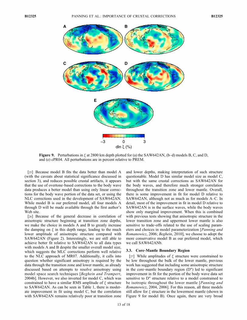
[27] While amplitudes of x structure were constrained tobe low throughout the bulk of the lower mantle, previouswork has suggested that including some anisotropic structurein the core‐mantle boundary region (D″) led to significantimprovement in fit for the portion of the body wave data setsensitive to D″ structure relative to a model constrained tobe isotropic throughout the lower mantle [Panning andRomanowicz, 2004, 2006]. For this reason, all three modelsstill allow for x structure in the lowermost mantle (shown inFigure 9 for model B). Once again, there are very broad

Figure 9. Perturbations in x at 2800 km depth plotted for (a) the SAW642AN, (b–d) models B, C, and D,and (e) cPR04. All perturbations are in percent relative to PREM.


13 of 18

similarities with the structure resolved in SAW642AN,but there are significant differences, as emphasized by therelatively low correlation values ranging between 0.4 and0.5 for models B and C relative to SAW642AN (Figure 6).Interestingly, some of the largest apparent visual differences,

such as the band of positive x running through the centralPacific, and the negative x under much of Asia appear moresimilar to the model PR04 developed with only linear cor-rections (Figure 9a).

Figure 10. Same as Figure 6 but plotting correlations relative to model PR04 for SAW642AN andmodels B, C, and D (dashed lines with symbols as defined in the legend).


14 of 18

[28] In order to explore this further, we calculated corre-lations of SAW642AN and models B and C to PR04 up tothe maximum resolution of that model, spherical harmonicdegree 8 (Figure 10). While SAW642AN is generally dec-orrelated from PR04 throughout the lower mantle, models Band C show much greater correlation, ranging from 0.6 to 0.7with the exception of the structure resolved in the lowermostspline in both models.[29] Another concern in this depth range is resolution. The

structure in this depth range is primarily controlled by SKSand core diffracted S phases, as well as some multiple ScSphases. While coverage is in general better in the lower-most mantle than in much of the midmantle [Panning andRomanowicz, 2006, Figure 2], checkerboard resolution testssuggest that there may be some contamination due to iso-tropic velocity structure (see auxiliary material).[30] Such concerns and the differences between the models

of D″ anisotropy developed with three different crustal cor-rection choices could also bring into question the signal ofspherically averaged positive x in this depth range, which wepreviously considered to be a robust conclusion [Panning andRomanowicz, 2004, 2006]. While contamination from iso-tropic velocity seems to be unlikely, as there is no compar-able strong mean signal in the VS profile, we can see that theaverage signature is almost absent in model B (Figure 11),and is shifted to shallower depths in model C. This is, ofcourse, a consequence of the choice to more heavily dampanisotropic structure at transition zone and greater depthsin model B relative to SAW642AN or model C. Additionally,as pointed out before, the applicability of the MLC approachto body waves is inherently problematic, and so previousmodels of lower mantle anisotropic structure may actuallybe preferred. Model D uses the previous NLC corrections forthe body waves, and results in D″ much more similar toSAW642AN, both in terms of 3‐D structure and 1‐D average.

Finally, there are multiple independent lines of evidence forwidespread presence of VSH > VSV in D″ based on detailedanalysis of waveforms sampling the region [e.g., Lay et al.,1998]. In general, however, it appears that the specific de-tails of D″ anisotropy in a global tomographic model are quitesensitive to the choice of crustal corrections, and thereforepotentially problematic to interpret.

4. Discussion

[31] The sensitivity of resolved mantle anisotropic struc-ture to the method of crustal correction used implies thatcrustal corrections may currently be a limiting factor forimproved resolution and agreement between models ofmantle anisotropy. Isotropic structure appears to be rela-tively robust as indicated by its greater stability in this studyas well as the broad convergence of models from differentresearch groups using different data sets and differentapproaches to crustal structure. However, it is apparent thatmoving to finer resolution or including second‐order struc-ture such as anisotropy or attenuation will require veryaccurate crustal corrections. The difficulties presented bycrustal structure for radially anisotropic models as in thisstudy also likely indicate that crustal corrections will beeven more important for robust determination of modelsusing more ambitious anisotropic parameterizations includ-ing arbitrarily oriented symmetry axes [Montagner andNataf, 1988; Sieminski et al., 2007; Panning and Nolet,2008].[32] Of course, one avenue of improving crustal corrections

has to be improving our knowledge of the real structure of theEarth’s crust. A recent study by Ferreira et al. [2010] showeddifferences between radially anisotropic models developedusing different models for the crust, particularly in the top100 km of the mantle. In this case, the methodology of using

Figure 11. Spherically symmetric x signature through the mantle for PREM (thin black dashed line) aswell as models PR04 (solid black line), SAW642AN (medium dashed line), model B (dash‐dotted line),model C (dotted line), and model D (thick dashed line).


15 of 18

local eigenfunction calculations along a great circle path [e.g.,Boschi and Ekström, 2002] was used to correct a large data setof fundamental and overtone surface wave phase velocitymeasurements for three different published global crustalmodels. The resulting models had some noticeable differences,particularly in the 100 km depth range, while differences incrustal models had as much impact on fit to the data asincluding radial anisotropy. For long‐period waveform datasets such as the one used in this modeling, improving crustalmodels may partially be accomplished by moving frommodels derived from more localized studies and tectonicinference, such as CRUST5.1 [Mooney et al., 1998] andCRUST2.0 [Bassin et al., 2000] to models derived specifi-cally from global surface wave data sets [e.g., Meier et al.,2007], although Ferreira et al. [2010] suggests that modelmay actually result in a poorer fit. However, SAW642ANand the models discussed in this study are derived fromdifferent implementations of nonlinear crustal corrections,but starting from the same crustal model, CRUST2.0. Thedifferences between the models implies that we need to notonly seek to improve the crustal models used for correction,but importantly to focus on which methods of applyingcrustal corrections are up to the task.[33] Allowing for inversion for further Moho perturbations

is another specific methodological tool used in previousmodels developed using NACT to improve crustal correc-tions [Li and Romanowicz, 1996; Mégnin and Romanowicz,2000]. These Moho perturbations were not intended to beinterpreted, but rather to act as a ‘trash can’ in which to dumpunmodeled crustal structure. This particular approach is notwell‐suited for use with the MLC approach, however. TheMLC method explicitly uses multiple sets of Moho pertur-bations for different mode types, and thus an inversion for anew single set of Moho perturbations is poorly formed, andwould throw out the nonlinear crustal corrections for anyfurther iteration. However, such an approach was tested aswell (see auxiliary material) but did not lead to significantchanges in the output models or fit to the data.[34] The improved data fit and removal of apparent crustal

artifacts relative to SAW642AN are strong evidence that theMLC correction approach performs better for this data setthan the NLC corrections used in the earlier model. Inter-estingly, this improved fit and removal of apparent crustalartifacts seems to require the MLC corrections be applied toboth the surface waves and body waves in the data set, asmodel D, which used the NLC corrections for the body waveshas similar data fit and radial correlation functions to SA-W642AN. It is not clear, however, exactly how to explain thisdifference. Both methods attempt to account for the nonlineareffects of crustal structure modeled as boundary perturbationsof the Moho and surface topography. Only the NLCapproach, however, directly includes the effect of differentcrustal structure on the sensitivity kernels to deep structure,which would seem to offer improvement relative to theapproach used here. However, the higher computational costsof the NLC approach did lead to the use of a smaller set ofregionalized models (5 versus 7 in this study), and it is pos-sible some of the differences may result from that. It is alsopossible that the improvement results from some sort offortuitous cancelation of errors, where any errors introducedby the MLC approach are somehow complementary to errorsintroduced through any inadequacies of CRUST2.0. Finally,

it is also possible that there was some error in the imple-mentation of NLC in the development of SAW642AN. Fur-ther study is warranted in order to understand this, but theway forward has to include better ways of fully incorporatingthe nonlinear effect of crustal structure on the waveforms.One possibility for this is to utilize numerical tools such as thespectral element method [e.g., Komatitsch and Vilotte, 1998]in the forward calculations which would incorporate allnonlinear effects on the wavefield provided we have accurateenough crustal models, while still using analytical approachesfor the partial derivatives used in the inversion (V. Lekićand B. Romanowicz, Inferring upper mantle structure by fullwaveform tomography with the spectral element method,submitted to Geophysical Journal International, 2010).Another avenue which will require taking advantage of ever‐increasing computational power is to utilize a fully numericalinverse approach such as the adjoint inversion proposed byTromp et al. [2005]. While many recent studies have focusedon improvements to tomography based upon the use of 3‐Dfinite frequency sensitivity kernels [Montelli et al., 2006;Zhou et al., 2006], using such approaches for crustal structurewill likely not offer significant improvement, as these remainstrictly a linear approach [e.g., Panning et al., 2009], and assuch are likely inadequate to correct for the effects of crustalstructure.[35] While there is strong evidence that the preferred model

in this study, SAW642ANb, is an improvement relative toSAW642AN, we need to consider very carefully whether theanisotropic structure at all depth ranges can be consideredreliable. Clearly the overall fit to the data has improved, andthe isotropic model in particular appears to show less indi-cation of crustal contamination. Routine tests of modelquality, such as resolution matrix checkerboard tests andbootstrap error maps (see auxiliary material), indicate resultsvery similar to SAW642AN for the isotropic structure,although the apparent resolution of lower mantle anisotropicstructure is naturally reduced because we choose to increasedamping for this depth range. Additionally, lower mantlestructure obviously depends most strongly on the bodywave data set, and despite the improved fits, there are stilltheoretical reasons to question the application of the MLCapproach to body waves due to the implicit assumption ofself‐coupling of modes. Attempting to use MLC for thesurface waves and NLC for the body waves (model D),however, does not show the apparent reduction in artifactsshown in models B and C. Perhaps the difference is par-tially related to the larger number of regionalized modelspossible in the MLC approach, but this is not certain. Takentogether, these concerns indicate that there remains a lot ofroom for improvement in global anisotropic models, partic-ularly at large depths, and that interpretation of anisotropicstructure below upper mantle depths should not be takenlightly.

5. Conclusions

[36] We have applied a new method of crustal correctionsto the same three‐component waveform data set used in thecreation of SAW642AN. By comparingmodels derived usingdifferent crustal corrections, we have shown that crustalcorrections have the potential for substantially affecting theretrieved anisotropic structure even in the lower mantle. Our


16 of 18

preferred model, SAW642ANb, shows improved data fit andevidence of fewer crustal artifacts. Because of the sensitivityof resolved anisotropic structure at transition zone and greaterdepths to the choice of crustal corrections, we prefer a modelwith anisotropic structure more strongly damped than inprevious modeling. Despite the overall smaller model sizeof this new model (as determined from RMS amplitude ofstructure as a function of depth), the fit to all data types isimproved relative to SAW642AN.

[37] Acknowledgments. This research was partially supportedby NSF grant EAR‐0911414. Support for V.L. provided in part by NSFGraduate Fellowship.

ReferencesBassin, C., G. Laske, and G. Masters (2000), The current limits of resolu-tion for surface wave tomography in North America, Eos Trans. AGU,81(48), Fall Meet. Suppl., Abstract S12A‐03.

Becker, T., B. Kustowski, and G. Ekström (2008), Radial seismic anisot-ropy as a constraint for upper mantle rheology, Earth Planet. Sci. Lett.,267, 213–227, doi:10.1016/j.epsl.2007.11.038.

Beghein, C. (2010), Radial anisotropy and prior petrological constraints:A comparative study, J. Geophys. Res., 115, B03303, doi:10.1029/2008JB005842.

Beghein, C., and J. Trampert (2004a), Probability density functions forradial anisotropy for fundamental mode surface wave data and the Neigh-bourhood Algorithm, Geophys. J. Int., 157, 1163–1174, doi:10.1111/j.1365-246X.2004.02235.x.

Beghein, C., and J. Trampert (2004b), Probability density functions forradial anisotropy: Implications for the upper 1200 km of the Earth, EarthPlanet. Sci. Lett., 217, 151–162, doi:10.1016/S0012-821X(03)00575-2.

Beghein, C., J. Resovsky, and R. van der Hilst (2008), The signal ofmantle anisotropy in the coupling of normal modes, Geophys. J. Int.,175, 1209–1234, doi:10.1111/j.1365-246X.2008.03970.x.

Boschi, L., and A. Dziewonski (2000), Whole Earth tomography fromdelay times of P, PcP, and PKP phases: Lateral heterogeneities in theouter core or radial anisotropy in the mantle?, J. Geophys. Res.,105(B6), 13,675–13,696, doi:10.1029/2000JB900059.

Boschi, L., and G. Ekström (2002), New images of the Earth’s uppermantle from measurements of surface wave phase velocity anomalies,J. Geophys. Res., 107(B4), 2059, doi:10.1029/2000JB000059.

Bozdağ, E., and J. Trampert (2008), On crustal corrections in surface wavetomography, Geophys. J. Int., 172, 1066–1082, doi:10.1111/j.1365-246X.2007.03690.x.

Ferreira, A. M. G., J. H. Woodhouse, K. Visser, and J. Trampert (2010),On the robustness of global radially anisotropic surface wave tomography,J. Geophys. Res., 115, B04313, doi:10.1029/2009JB006716.

Gu, Y., A. Dziewonski, and G. Ekström (2003), Simultaneous inversion formantle shear velocity and topography of transition zone discontinuities,Geophys. J. Int., 154, 559–583, doi:10.1046/j.1365-246X.2003.01967.x.

Gung, Y., M. Panning, and B. Romanowicz (2003), Global anisotropyand the thickness of continents, Nature, 422, 707–711, doi:10.1038/nature01559.

Houser, C., G. Masters, P. Shearer, and G. Laske (2008), Shear andcompressional velocity models of the mantle from cluster analysis oflong‐period waveforms, Geophys. J. Int., 174, 195–212, doi:10.1111/j.1365-246X.2008.03763.x.

Kaminski, E., and N. Ribe (2001), A kinematic model for recrystallizationand texture development in olivine polycrystals, Earth Planet. Sci. Lett.,189, 253–267, doi:10.1016/S0012-821X(01)00356-9.

Karato, S.‐I., H. Jung, I. Katayama, and P. Skemer (2008), Geodynamicsignificance of seismic anisotropy of the upper mantle: New insightsfrom laboratory studies, Annu. Rev. Earth Planet. Sci., 36, 59–95,doi:10.1146/annurev.earth.36.031207.124120.

Komatitsch, D., and J.‐P. Vilotte (1998), The spectral‐element method: anefficient tool to simulate the seismic response of 2D and 3D geologicalstructures, Bull. Seismol. Soc. Am., 88(2), 368–392.

Kustowski, B., A. Dziewoński, and G. Ekström (2007), Nonlinear crustalcorrections for normal‐mode seismograms, Bull. Seismol. Soc. Am.,97(5), 1756–1762, doi:10.1785/0120070041.

Kustowski, B., G. Ekström, and A. M. Dziewoński (2008), Anisotropicshear wave velocity structure of the Earth’s mantle: A global model,J. Geophys. Res., 113, B06306, doi:10.1029/2007JB005169.

Lay, T., Q. Williams, E. Garnero, L. Kellogg, and M. Wysession (1998),Seismic wave anisotropy in the D″ region and its implications, in TheCore‐Mantle Boundary Region,Geodyn. Ser., vol. 28, edited byM.Gurniset al., pp. 299–318, AGU, Washington, D. C.

Lekić, V., M. Panning, and B. Romanowicz (2010), A simple method forimproving crustal corrections in waveform tomography, Geophys. J. Int.,182, 265–278, doi:10.1111/j.1365-246X.2010.04602.x.

Li, C., R. van der Hilst, and M. Toksöz (2006), Constraining P‐wave veloc-ity variation in the upper mantle beneath Southeast Asia, Phys. EarthPlanet. Inter., 154, 180–195, doi:10.1016/j.pepi.2005.09.008.

Li, X.‐D., and B. Romanowicz (1995), Comparison of global waveforminversions with and without considering cross‐branch modal coupling,Geophys. J. Int., 121, 695–709, doi:10.1111/j.1365-246X.1995.tb06432.x.

Li, X.‐D., and B. Romanowicz (1996), Global mantle shear velocity modeldeveloped using nonlinear asymptotic coupling theory, J. Geophys. Res.,101(B10), 22,245–22,272, doi:10.1029/96JB01306.

Marone, F., and B. Romanowicz (2007), Non‐linear crustal correctionin high‐resolution regional waveform seismic tomography, Geophys.J. Int., 170(1), 460–467, doi:10.1111/j.1365-246X.2007.03399.x.

Mégnin, C., and B. Romanowicz (1999), The effect of theoretical formal-ism and data selection scheme on mantle models derived from waveformtomography, Geophys. J. Int., 138, 366–380, doi:10.1046/j.1365-246X.1999.00869.x.

Mégnin, C., and B. Romanowicz (2000), The 3D shear velocity structure ofthe mantle from the inversion of body, surface, and higher mode wave-forms, Geophys. J . Int . , 143 , 709–728, doi:10.1046/j .1365-246X.2000.00298.x.

Meier, U., A. Curtis, and J. Trampert (2007), Fully nonlinear inversion offundamental mode surface waves for a global crustal model, Geophys.Res. Lett., 34, L16304, doi:10.1029/2007GL030989.

Montagner, J.‐P., and N. Jobert (1988), Vectorial tomography: II. Applica-tion to the Indian Ocean, Geophys. J. R. Astron. Soc., 94, 309–344.

Montagner, J.‐P., and H.‐C. Nataf (1988), Vectorial tomography: I. Theory,Geophys. J. R. Astron. Soc., 94, 295–307.

Montelli, R., G. Nolet, F. Dahlen, G. Masters, E. Engdahl, and S.‐H. Hung(2004), Finite‐frequency tomography reveals a variety of plumes in themantle, Science, 303, 338–343, doi:10.1126/science.1092485.

Montelli, R., G. Nolet, F. Dahlen, and G. Masters (2006), A catalogue ofdeep mantle plumes: New results from finite‐frequency tomography,Geochem. Geophys. Geosyst., 7, Q11007, doi:10.1029/2006GC001248.

Mooney, W., G. Laske, and G. Masters (1998), CRUST 5.1: A globalcrustal model at 5 × 5 degrees, J. Geophys. Res., 103, 727–747,doi:10.1029/97JB02122.

Panning, M., and G. Nolet (2008), Surface wave tomography for azimuthalanisotropy in a strongly reduced parameter space, Geophys. J. Int.,174(2), 629–648, doi:10.1111/j.1365-246X.2008.03833.x.

Panning, M., and B. Romanowicz (2004), Inferences on flow at the base ofEarth’s mantle based on seismic anisotropy, Science, 303, 351–353,doi:10.1126/science.1091524.

Panning, M., and B. Romanowicz (2006), A three‐dimensional radiallyanisotropic model of shear velocity in the whole mantle, Geophys.J. Int., 167, 361–379, doi:10.1111/j.1365-246X.2006.03100.x.

Panning, M., Y. Capdeville, and B. Romanowicz (2009), Seismic wave-form modelling in a 3‐D Earth using the Born approximation: Potentialshortcomings and a remedy, Geophys. J. Int., 177, 161–178, doi:10.1111/j.1365-246X.2008.04050.x.

Park, J. (1993), The sensitivity of seismic free oscillations to upper mantleanisotropy: 1. Zonal symmetry, J. Geophys. Res., 98(B11), 19,933–19,949, doi:10.1029/93JB02177.

Ritsema, J., H. J. van Heijst, and J. H. Woodhouse (2004), Global transitionzone tomography, J. Geophys. Res., 109, B02302, doi:10.1029/2003JB002610.

Romanowicz, B., M. Panning, Y. Gung, and Y. Capdeville (2008), On thecomputation of long period seismograms in a 3D Earth using normalmode based approximations, Geophys. J. Int., 175(2), 520–536,doi:10.1111/j.1365-246X.2008.03914.x.

Sieminski, A., Q. Liu, J. Trampert, and J. Tromp (2007), Finite‐frequencysensitivity of surface waves to anisotropy based upon adjoint methods,Geophys. J. Int., 168, 1153–1174, doi:10.1111/j.1365-246X.2006.03261.x.

Simmons, N., A. Forte, and S. Grand (2009), Joint seismic, geodynamicand mineral physical constraints on three‐dimensional mantle heteroge-neity: Implications for the relative importance of thermal versus compo-sitional heterogeneity, Geophys. J. Int., 177, 1284–1304, doi:10.1111/j.1365-246X.2009.04133.x.

Tromp, J., C. Tape, and Q. Liu (2005), Seismic tomography, adjoint meth-ods, time reversal and banana‐doughnut kernels, Geophys. J. Int., 160,195–216, doi:10.1111/j.1365-246X.2004.02453.x.


17 of 18

Wang, Z., and F. Dahlen (1995), Spherical‐spline parameterization of three‐dimensional Earth models, Geophys. Res. Lett., 22(22), 3099–3102,doi:10.1029/95GL03080.

Zhou, Y., G. Nolet, F. Dahlen, and G. Laske (2006), Global upper‐mantlestructure from finite‐frequency surface‐wave tomography, J. Geophys.Res., 111, B04304, doi:10.1029/2005JB003677.

V. Lekić, Department of Geological Sciences, Brown University,324 Brook St., Providence, RI 02912, USA.

M. P. Panning, Department of Geological Sciences, University ofFlorida, 241 Williamson Hall, PO Box 112120, Gainesville, FL 32611,USA. ([email protected])B. A. Romanowicz, Berkeley Seismological Laboratory, University of

California, McCone Hall 215, Berkeley, CA 94720, USA.


18 of 18

importance of crustal corrections in the...

Documents