implementation of the rose algebra: efï¬cient algorithms for
TRANSCRIPT

Implementation of the ROSE Algebra:
Efficient Algorithms for Realm-Based Spatial Data Types
Abstract: The ROSE algebra, defined earlier, is a system of spatial data types for use in spatial data-base systems. It offers data types to represent points, lines, and regions in the plane together with acomprehensive set of operations; semantics of types and operations have been formally defined. Val-ues of these data types have a quite general structure, e.g. an object of typeregions may consist ofseveral polygons with holes. All ROSE objects arerealm-based which means all points and verticesof objects lie on an integer grid and no two distinct line segments of any two objects intersect in theirinterior. In this paper we describe the implementation of the ROSE algebra, providing data structuresfor the types and newrealm-based geometric algorithms for the operations. The main techniques usedare (parallel) traversal of objects, plane-sweep, and graph algorithms. All algorithms are analyzedwith respect to their worst case time and space requirements. Due to the realm properties, these algo-rithms are relatively simple, efficient, and numerically completely robust. All data structures and al-gorithms have indeed been implemented in theROSE system; the Modula-2 source code is freelyavailable from the authors for study or use.
Keywords: Spatial data types, algebra, realm, finite resolution, numerical robustness, efficient algo-rithms, plane sweep, ROSE.
This work was supported by the DFG (Deutsche Forschungsgemeinschaft) under grant Gu 293/1-2.
Ralf Hartmut Güting
Praktische Informatik IVFernuniversität Hagen
D-58084 HagenGERMANY
Thomas de Ridder
Praktische Informatik IIIFernuniversität Hagen
D-58084 HagenGERMANY
Markus Schneider
Praktische Informatik IVFernuniversität Hagen
D-58084 HagenGERMANY

− 1 −
1 Introduction
We consider aspatial database system to be a full-fledged database system with additional capabilitiesfor representing, querying, and manipulating geometric data (for a survey see [Gü94]). Such a systemprovides the underlying database technology needed to support applications such asgeographic in-formation systems and others. Spatial data types likepoint, line, andregion provide a fundamental ab-straction for modeling the structure of geometric entities, their relationships, properties, and opera-tions. Their definition and implementation is probably the most fundamental issue in the developmentof spatial database systems.
There have been quite a few proposals for systems of spatial data types and operations, orspatial al-gebras; they have been embedded into query languages, implemented in prototype systems, and someof them have been defined formally. For a discussion and references see [GüS93b, Gü94]. This papercontinues the development of one such proposal, theROSE algebra [GüS93b], which has a numberof interesting features: (i) it offers (values of) data types of a very general structure, (ii) has a completeformal definition of the semantics of types and operations, (iii) has a discrete geometric basis (so-calledrealms, see below) which allows for a correct and robust implementation in terms of integerarithmetics, (iv)treats consistency between distinct geometric objects with common parts, and (v) hasa general object model interface which allows it to cooperate with different kinds of database systems.
The development of the ROSE algebra so far consists of three steps: (1) the concept of arealm[GüS93a] as adiscrete geometric basis, (2) the formal definition of theROSE algebra itself offeringrealm-based spatial data types and operations [GüS93b], and (3)theROSE system as an implementa-tion of the ROSE algebra, which realizes its types and operations by providing efficient data structuresand algorithms defined over a discrete grid. This third step is the subject of this paper. Let us brieflyreview the first two steps.
A realm conceptually describes the complete underlying geometry of a particular application space intwo dimensions. Formally, a realm is a finite set of points and line segments over a discrete grid (seeFigure 1(a)) such that (i) each point and each end point of a line segment is a grid point, (ii) each endpoint of a realm segment is also a point of the realm, (iii) no realm point lies within a realm segment(which means on it without being an end point), and (iv) no two realm segments intersect except attheir end points. The idea is now to construct the geometries of spatial objects by composing themfrom realm primitives (see Figure 1(b)). The realm concept solves numerical robustness and topolog-ical correctness problems, enforces geometric consistency of related spatial objects, and enables oneto formally define spatial data types or algebras on top of it that enjoy nice closure properties not onlyin theory but also in an implementation.
Figure1
A BC
D
(a) Example of a realm (b) Realm objects over the realm in (a)
− 2 −
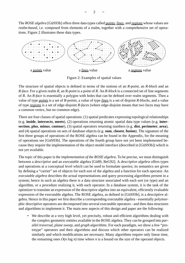
TheROSE algebra [GüS93b] offers three data types calledpoints, lines, andregions whose values arerealm-based, i.e. composed from elements of a realm, together with a comprehensive set of opera-tions. Figure 2 illustrates these data types.
The structure of spatial objects is defined in terms of the notions of anR-point, anR-block and anR-face. For a given realmR, anR-point is a point ofR. An R-block is a connected set of line segmentsof R. An R-face is essentially a polygon with holes that can be defined over realm segments. Then avalue of typepoints is a set ofR-points, a value of typelines is a set of disjointR-blocks, and a valueof typeregions is a set of edge-disjointR-faces (where edge-disjoint means that two faces may havea common vertex, but no common edge).
There are four classes of spatial operations: (1) spatial predicates expressing topological relationships(e.g.inside, intersects, meets), (2)operations returning atomic spatial data type values (e.g.inter-section, plus, minus, contour), (3) spatial operators returning numbers (e.g.dist, perimeter, area),and (4) spatial operations on sets of database objects (e.g.sum, closest, fusion). The signature of thefirst three groups of operations of the ROSE algebra can be found in the Appendix, for the meaningof operations see [GüS93b]. The operations of the fourth group have not yet been implemented be-cause they require the implementation of the object model interface (described in [GüS93b]) which isnot yet available.
The topic of this paper is theimplementation of the ROSE algebra. To be precise, we must distinguishbetween adescriptive and anexecutable algebra [Gü89, BeG92]. Adescriptive algebra offers typesand operations at a conceptual level which can be used to formulate queries; its semantics are givenby defining a “carrier” set of objects for each sort of the algebra and a function for each operator. Anexecutable algebra describes the actual representations and query processing algorithms present in asystem; hence in such an algebra there is a data structure associated with each sort (or type) and analgorithm, or a procedure realizing it, with each operator. In a database system, it is the task of theoptimizer to translate an expression of the descriptive algebra into an equivalent, efficiently evaluableexpression of the executable algebra. The ROSE algebra, as defined in [GüS93b], is a descriptive al-gebra. Hence in this paper we first describe a corresponding executable algebra - essentially polymor-phic descriptive operators are decomposed into several executable operators - and then data structuresand algorithms to implement it. The main new aspects of this design and paper are the following:
• We describe at a very high level, yet precisely, robust and efficient algorithms dealing withthe complex geometric entities available in the ROSE algebra. They can be grouped intopar-allel traversal, plane sweep, andgraph algorithms. For each paradigm, we show a few “pro-totype” operators and their algorithms and discuss which other operators can be realizedsimilarly and which modifications are necessary. Many algorithms require only linear time,the remaining onesO(n log n) time wheren is a bound on the size of the operand objects.
a points value a lines value a regions value
Figure 2: Examples of spatial values

− 3 −
• All spatial objects processed by the operations are realm-based, i.e., they are defined over adiscrete basis and in particular no two segments intersect within their interiors and no pointlies within a segment. These properties can be exploited for designing efficient geometric al-gorithms. For example, many operations can now be realized through a simple parallel tra-versal for which otherwise more complex and expensive plane sweep algorithms would beneeded. When plane sweep is needed, it is simpler because no intersection points of segmentscan be discovered during the sweep (e.g., a static sweep event structure can be used).
• In contrast to traditional papers on algorithms, the focus is not on finding the most efficientalgorithm for one single problem (operation), but rather on considering a spatial algebra asa whole, and on reconciling the various requirements posed by different algorithms within asingle data structure for each type. We are not aware that implementations of complete spa-tial algebras have been described before in a similar manner.
• The implementation is designed for use in a spatial database system. In particular, represen-tations for spatial data types do not use pointer data structures in main memory, but are allembedded into compact storage areas which can be efficiently transferred between a mainmemory buffer and disk. Data structures are also designed to allow for realm updates.
• The ROSE system has actually been implemented and is running; the complete source codeis available from the authors for study or use [Ri95]. The implementation was done in Mod-ula-2 for UNIX systems. We feel it is important to make such well-designed “modules” forspatial DBMS systems available to the research community.
The importance of afinite-precision / finite-resolution computational geometry, as described in thispaper, defined on a uniform, discrete grid such that points, end points of line segments, vertices ofpolygons etc. have integer coordinates instead of arbitrary floating-point coordinates, has been em-phasized by Greene and Yao [GrY86] as well as Yao [Ya92]. Finite-precision geometry has so far onlybeen studied by a few researchers (overviews can be found in [KeK81, Ov88b, Ov88c]). Problemsconsidered are, for example, the nearest neighbour searching problem [KaM85], range searching ona grid [Ov88a, Ov88b], the point location problem [Mü85], the computation of rectangle intersectionsand maximal elements by divide-and-conquer [KaO88b], computing the convex hull of a set of points,reporting all intersections of a set of arbitrarily oriented line segments, and the calculation of rectangleintersections and maximal elements by using the plane-sweep technique [KaO88a, Ov88b]. To ourknowledge, geometric algorithms over a discrete domain for more complex structures like those ofthe ROSE algebra have not been described in the literature.
The paper is structured as follows: In Section 2 an executable algebra is designed for the given de-scriptive ROSE algebra. In Section 3 we give a high-level specification of data structures for the rep-resentation of ROSE objects which provides a basis for the subsequent description of algorithms. Sec-tion 4 introducesrealm-based geometric algorithms for the implementation of ROSE operations. Sec-tion 5 shows the actual data structures used and discusses some important implementation concepts.
2 Descriptive and Executable ROSE Algebra
In this section we develop an executable algebra for the given descriptive ROSE algebra. Essentiallythis means that we have to decompose each polymorphic descriptive operator into corresponding ex-ecutable operators for the possible combinations of data types. Both algebras usesecond-order signa-ture [Gü93] as the underlying formalism. Second-order signature allows one to define a type systemtogether with an algebra over that type system. In particular, it is possible to describe polymorphic
− 4 −
operations by quantification overkinds. For the purpose ofthis paper it suffices to view kinds just astype sets; the two relevant sets are EXT = {lines, regions} and GEO = {points, lines, regions}. Hereare a few examples of spatial predicates of the ROSE algebra:
∀ geo in GEO.∀ ext1, ext2 in EXT. ∀ area in regionsarea-disjoint.geo × geo → bool =, ≠, disjointgeo × regions → bool insideext1 × ext2 → bool intersectsarea × area → bool adjacent, encloses
Heregeo is a type variable ranging over the three types in kind GEO so that the first three operationscan compare two values of equal type and theinside operation can compare apoints, alines, or are-gions value with aregions value. Theintersects operation can be applied to two values of the sameor different type within kind EXT. The notationregionsarea-disjoint is an attempt to capture the structureof partitions of the plane (into disjoint regions) in the type system. It ensures that the two operandsgiven to theadjacent orencloses operator are two regions taken from the same partition of the plane,hence they are either disjoint or equal; for details see [GüS93b]. For the executable algebra this is notrelevant and we can introduce executable operators with functionalityregions × regions → bool.
In the executable algebra, we generally need different algorithms for the different data types. For ex-ample, it is obvious that an algorithm which examines the disjointness of twopoints objects will bedifferent from an algorithm which determines whether tworegions objects overlap. Hence the de-scriptive operatordisjoint is mapped to the three executable operators:
points × points → bool pp_disjointlines × lines → bool ll_disjointregions × regions → bool rr_disjoint
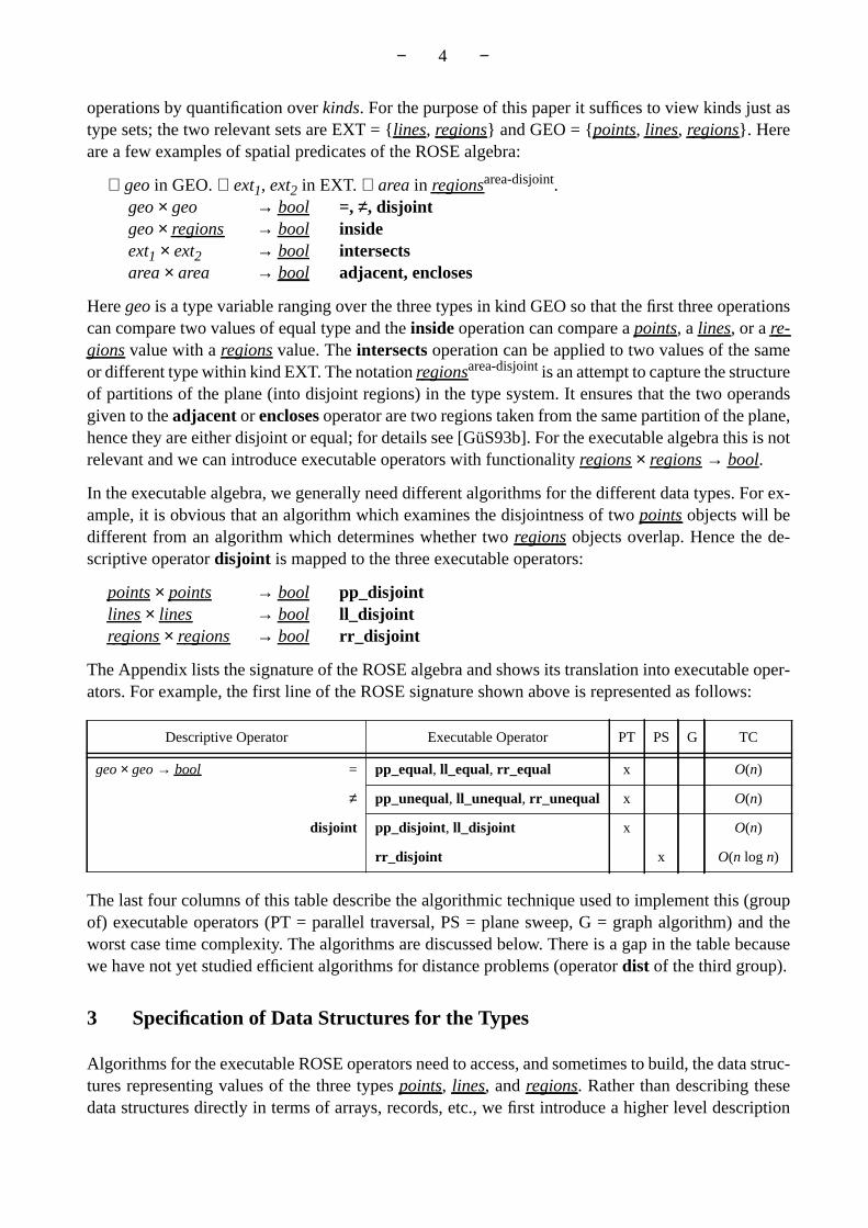
The Appendix lists the signature of the ROSE algebra and shows its translation into executable oper-ators.For example, the first line of the ROSE signature shown above is represented as follows:
The last four columns of this table describe the algorithmic technique used to implement this (groupof) executable operators (PT = parallel traversal, PS = plane sweep, G = graph algorithm) and theworst case time complexity. The algorithms are discussed below. There is a gap in the table becausewe have not yet studied efficient algorithms for distance problems (operatordist of the third group).
3 Specification of Data Structures for the Types
Algorithms for the executable ROSE operators need to access, and sometimes to build, the data struc-tures representing values of the three typespoints, lines, andregions. Rather than describing thesedata structures directly in terms of arrays, records, etc., we first introduce a higher level description
Descriptive Operator Executable Operator PT PS G TC
geo × geo → bool = pp_equal, ll_equal, rr_equal x O(n)
≠ pp_unequal, ll_unequal, rr_unequal x O(n)
disjoint pp_disjoint, ll_disjoint x O(n)
rr_disjoint x O(n log n)

− 5 −
which offers suitable access and construction operations to be used in the algorithms. Basically, wedefine a little abstract data type for each of the three data structures. In a second step, one can thendesign and implement the data structure itself.
The specification of an abstract data type consists of a many-sorted signature together with a set oflaws, or equations, defining the behaviour of operations. To be precise, we use a slightly differentspecification method sometimes called “denotational specification” (e.g. [Kl83]). It simply means thatwe assign semantics to the sorts and operations of the many-sorted signature directly by defining car-rier sets for the sorts and functions for the operations on these carrier sets, i.e., we define a little alge-bra for each of the three data structures representing points, lines, or regions values, respectively. Inother words, we give a concrete mathematical model for the data type instead of a set of laws. In fact,the whole ROSE algebra itself has been defined by the same method.
For most executable operators it turns out to be sufficient to regard a spatial object as an ordered se-quence of elements where it is possible to access these elements consecutively and to insert a new el-ement into the sequence. Hence this is our basic strategy for modeling the three data structures.
Before we can introduce the algebra points, a few notations are needed. Realms and realm-based spa-tial objects are defined over a finite discrete space N × N with N = {0, ..., m − 1} ⊆ N. PN = {(x, y) |x ∈ N, y ∈ N} denotes the set of all N-points. Furthermore, an (x, y)-lexicographic order is assumedon PN which is defined as p1 < p2 ⇔ x1 < x2 ∨ (x1 = x2 ∧ y1 < y2).
algebra points
sorts points, PN, bool
ops new : → pointsselect_first : points → pointsselect_next : points → pointsend_of_pt : points → boolget_pt : points → PNinsert : points × PN → points
sets points = {(pos, < p1, ..., pn >) | pos ≥ 0; n ≥ 0; for 1 ≤ i ≤ n, pi ∈ PN; for 1 ≤ i < n, pi < pi+1}
functions Let P = (i, < p1, ..., pn >) ∈ points and p ∈ PN.new() = (0, ◊)
(1, < p1, ..., pn >) if n ≥ 1select_first(P) =
(0, ◊) otherwise (i + 1, < p1, ..., pn >) if 1 ≤ i < n
select_next(P) = (0, < p1, ..., pn >) otherwise
end_of_pt(P) = (i = 0) pi if 1 ≤ i ≤ n
get_pt(P) = undefined otherwise (j, < p1, ..., pn >) if ∃ j ∈ {1, ..., n}: p = pj
insert(P, p) = (1, < p, p1, ..., pn >) if p < p1 (n + 1, < p1, ..., pn, p>) if p > pn (j + 1, < p1, ..., pj, p, pj+1, ..., pn >) if ∃ j∈{1, ..., n-1}: pj < p < pj+1
end points.
− 6 −
Thesorts andops parts describe the syntax of the algebra, i.e., the signature. Thesets andfunctionsparts give the semantics in terms of carrier set and function definitions. The algebrapoints containsthe sortspoints (to be defined),PN, andbool. The carrier set of the sortpoints is defined as the set ofall ordered sequences <p1, ...,pn > of n N-points together with a pointer indicating a position withinthe sequence. The symbol◊ denotes the empty sequence. Functions manipulate such values, for ex-ample,select_first positions the pointerpos on the smallest element of the point sequence, andget_ptyields the point at the current position.
A crucial idea for the representation of the relatively complexlines andregions values, which is thebasis for most of our algorithms, is to regard them asordered sequences of halfsegments. Let SN ={( p, q) | p ∈ PN, q ∈ PN} denote the set ofN-segments. The equality of twoN-segmentss1 = (p1, q1)ands2 = (p2, q2) is defined ass1 = s2 ⇔ (p1 = p2 ∧ q1 = q2) ∨ (p1 = q2 ∧ p2 = q1). W. l. o. g. we nor-malizeSN by the assumption that∀ s ∈ SN : s = (p, q) ⇒ p < q which enables us to speak of aleft anda right end point of a segment. Let furtherHN = {(s, d) | s ∈ SN, d ∈ { left, right}} be the set ofhalf-segments. A halfsegmenth = (s, d) consists of anN-segments and a flagd emphasizing one of theN-segment’s end points which is called thedominating point of h. If d = left then the left (smaller) endpoint ofs is the dominating point ofh, andh is calledleft halfsegment. Otherwise, the right end pointof s is the dominating point ofh, andh is calledright halfsegment. Hence, eachN-segments is mappedto two halfsegments (s, left) and (s, right). Let dp be the function which yields the dominating pointof a halfsegment.
For two distinct halfsegmentsh1 andh2 with a common end pointp, letα be the enclosed angle suchthat 0 <α ≤ 180° (an overlapping ofh1 andh2 is excluded by the realm properties). Let a predicaterot be defined as follows:rot(h1, h2) is true iff h1 can be rotated aroundp throughα to overlaph2 incounter-clockwise direction. We can now define a complete order on halfsegments which is basicallythe (x, y)-lexicographic order by dominating points. For two halfsegmentsh1 = (s1, d1) andh2 =(s2, d2) it is:
h1 < h2 ⇔ dp(h1) < dp(h2) ∨ (dp(h1) = dp(h2) ∧ ((d1 = right ∧ d2 = left) ∨ (d1 = d2 ∧ rot(h1, h2))))
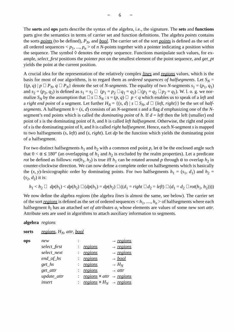
We now define the algebraregions (the algebralines is almost the same, see below). The carrier setof the sortregions is defined as the set of ordered sequences <h1, ....,hn > of halfsegments where eachhalfsegmenthi has an attachedset of attributes ai whose elements are values of some new sortattr.Attribute sets are used in algorithms to attach auxiliary information to segments.
algebra regions
sorts regions, HN, attr, bool
ops new : → regionsselect_first : regions → regionsselect_next : regions → regionsend_of_hs : regions → boolget_hs : regions → HNget_attr : regions → attrupdate_attr : regions × attr → regionsinsert : regions × HN → regions
− 7 −
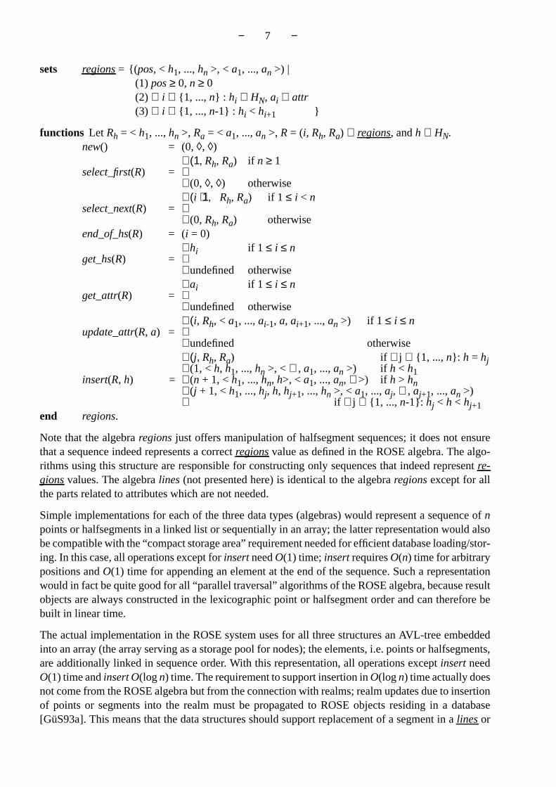
sets regions = {( pos, < h1, ...,hn >, <a1, ...,an >) |(1) pos ≥ 0, n ≥ 0(2) ∀ i ∈ {1, ..., n} : hi ∈ HN, ai ⊆ attr(3) ∀ i ∈ {1, ..., n-1} : hi < hi+1 }
functions Let Rh = < h1, ...,hn >, Ra = < a1, ...,an >, R = (i, Rh, Ra) ∈ regions, andh ∈ HN.new() = (0, ◊, ◊)
(1, Rh, Ra) if n ≥ 1select_first(R) =
(0, ◊, ◊) otherwise (i + 1, Rh, Ra) if 1 ≤ i < n
select_next(R) = (0, Rh, Ra) otherwise
end_of_hs(R) = (i = 0) hi if 1 ≤ i ≤ n
get_hs(R) = undefined otherwise ai if 1 ≤ i ≤ n
get_attr(R) = undefined otherwise (i, Rh, < a1, ...,ai-1, a, ai+1, ...,an >) if 1 ≤ i ≤ n
update_attr(R, a) = undefined otherwise (j, Rh, Ra) if ∃ j ∈ {1, ..., n}: h = hj (1, <h, h1, ...,hn >, <∅, a1, ...,an >) if h < h1
insert(R, h) = (n + 1, <h1, ...,hn, h>, < a1, ...,an, ∅>) if h > hn (j + 1, <h1, ...,hj, h, hj+1, ...,hn >, <a1, ...,aj, ∅, aj+1, ...,an >) if ∃ j ∈ {1, ..., n-1}: hj < h < hj+1
end regions.
Note that the algebraregions just offers manipulation of halfsegment sequences; it does not ensurethat a sequence indeed represents a correctregions value as defined in the ROSE algebra. The algo-rithms using this structure are responsible for constructing only sequences that indeed representre-gions values. The algebralines (not presented here) is identical to the algebraregions except for allthe parts related to attributes which are not needed.
Simple implementations for each of the three data types (algebras) would represent a sequence ofnpoints or halfsegments in a linked list or sequentially in an array; the latter representation would alsobe compatible with the “compact storage area” requirement needed for efficient database loading/stor-ing. In this case, all operations except forinsert needO(1) time;insert requiresO(n) time for arbitrarypositions andO(1) time for appending an element at the end of the sequence. Such a representationwould in fact be quite good for all “parallel traversal” algorithms of the ROSE algebra, because resultobjects are always constructed in the lexicographic point or halfsegment order and can therefore bebuilt in linear time.
The actual implementation in the ROSE system uses for all three structures an AVL-tree embeddedinto an array (the array serving as a storage pool for nodes); the elements, i.e. points or halfsegments,are additionally linked in sequence order. With this representation, all operations exceptinsert needO(1) time andinsert O(logn) time. The requirement to support insertion inO(logn) time actually doesnot come from the ROSE algebra but from the connection with realms; realm updates due to insertionof points or segments into the realm must be propagated to ROSE objects residing in a database[GüS93a]. This means that the data structures should support replacement of a segment in alines or

− 8 −
regions object by a chain of segments, i.e., the segment must be deleted and the replacement segmentsbe inserted into the structure. Unfortunately, a consequence of this is that the parallel traversal algo-rithms cannot construct the result objects in linear time any more, but need O(k log k) for this wherek is the size of the result object. This is a case of conflicting requirements, as mentioned in the intro-duction. On the other hand, deriving the internal structure of a lines or regions object (e.g. faces andholes) which is needed to complete the construction (see Section 5) requires O(k log k) time anyway.
4 Algorithms for the Executable Algebra
This section introduces realm-based geometric algorithms whose characteristic features are numeri-cal robustness, topological correctness, closure properties, and efficiency. Realm-based algorithmsare more efficient than their Euclidean counterparts. The design of these algorithms is based on tra-versal techniques, on the plane-sweep paradigm, and on graph theory. Realm-based geometry dealswith spatial objects that are defined over the same discrete domain and assumes that no two segmentsintersect within their interiors and that no point lies within a segment.
Executable operators are grouped by the applied algorithmic technique. For each group we show andexplain some example algorithms.
4.1 Algorithms with Simple or Parallel Object Traversal
A number of operators of the executable ROSE algebra can be realized by a simple or parallel travers-al (scan) through the point or halfsegment sequence of one or two objects. To simplify the descriptionof algorithms, for each possible combination of two spatial data types two operations are introducedwhich allow for a parallel traversal through two ordered sequences of elements (halfsegments, points).
As an example, we consider the two operations for two regions objects. The operationrr_select_first(R1, R2, object, status) selects the first halfsegment of each of the regions objects R1 andR2 (compare to the function select_first of algebra regions) and positions a logical pointer on both ofthem. The parameter object with possible values {none, first, second, both} indicates which of the twoobject representations contains the smaller halfsegment. If the value of object is none, no halfsegmentis selected, since R1 and R2 are empty. If it is first (second), the smaller halfsegment belongs to R1(R2). If it is both, the first halfsegments of R1 and R2 are identical. The parameter status with possiblevalues {end_of_none, end_of_first, end_of_second, end_of_both} describes the state of both halfseg-ment sequences. If the value of status is end_of_none, both objects still have halfsegments. If it isend_of_first (end_of_second), R1 (R2) is empty. If it is end_of_both, both object representations areempty.
The operation rr_select_next(R1, R2, object, status) searches for the next smaller halfsegment of R1and R2; parameters have the same meaning as for rr_select_first. Obviously, this is realized byselect_next operations of the two objects.
Both operations together allow one to scan in linear time two object representations like one orderedsequence. Analogous operations can be defined for two lines objects (ll_select_first, ll_select_next)and a lines and a regions object (lr_select_first, lr_select_next). For the comparison of halfsegmentswith points, the dominating points of the halfsegments are used so that points and lines objects

− 9 −
(pl_select_first, pl_select_next) as well aspoints andregions objects (pr_select_first, pr_select_next)can be treated in a similar way.
In the sequel we discuss algorithms for the operations (see algorithms below):
points × regions → bool pr_on_border_ofpoints × points → points pp_pluslines × lines → bool ll_intersects
Operatorpr_on_border_of determines whether all points of apoints object lie on the faces’ bound-aries of aregions object. Hence the algorithm checks whether for each pointp of apoints objectP(denoted asp ∈ P(P)) a halfsegmenth of aregions objectR (denotedh ∈ H(R)) exists whose domi-nating point is equal top. The while-loop of the algorithm is executed as long as no point is foundwhich is inP but not a dominating point of a halfsegment ofR and as long as none of the object se-quences is exceeded. For the predicate to betrue, termination of the while-loop must not have oc-curred because a point was found which is not on the boundary ofR (object ≠ first). This implies thattermination is due to reaching the end of one or both sequences, and the predicate istrue if this wasnot theregions sequence alone (status ≠ end_of_second).
Operatorpp_plus forms the union of twopoints objects. The algorithm just scans the point sequencesof the two objects and merges them into a newpoints object.
algorithm ll_intersectsinput: Two lines objectsL1 andL2output:true, if no common segment exists, but a com-
mon point which is not a meeting pointfalse, otherwise
beginll_select_first(L1, L2, object, status);if object = first then act_dp := dp(get_hs(L1))else if object = second then act_dp := dp(get_hs(L2))end-if;act_obj := object; found := false; count := 0;while (status = end_of_none) and (object ≠ both) do
ll_select_next(L1, L2, object, status);if (status ≠ end_of_both) and (object ≠ both) and
not found thenif object = first then
new_dp := dp(get_hs(L1))else if object = second then
new_dp := dp(get_hs(L2))end-if;if new_dp ≠ act_dp then (* new point *)
act_dp := new_dp; count := 0;act_obj := object;
else if object ≠ act_obj then (* object switch *)count := count + 1;act_obj := object;found := found or (count > 2);
end-if;end-if;
end-while;return found and (object ≠ both);
end ll_intersects.
algorithm pr_on_border_ofinput: A points objectP and aregions objectRoutput:true, if ∀ p ∈ P(P) ∃ h ∈ H(R) : p = dp(h)
false, otherwisebegin
pr_select_first(P, R, object, status);while (object ≠ first) and (status = end_of_none) do
pr_select_next(P, R, object, status);end-while;return (object ≠ first) and (status ≠ end_of_second)
end pr_on_border_of.
algorithm pp_plusinput: Two points objectsP1 andP2output:A points objectPnew containing all pointsbegin
Pnew := new();pp_select_first(P1, P2, object, status);while status ≠ end_of_both do
if object = first then p := get_pt(P1)else if object = second then p := get_pt(P2)else if object = both then p := get_pt(P1)end-if;Pnew := insert(Pnew, p);pp_select_next(P1, P2, object, status);
end-while;return Pnew
end pp_plus.

− 10 −
Operator ll_intersects examines whether two lines objects L1 and L2 intersect. According to the def-inition of the ROSE algebra it yields true if both objects have no common (half)segments but at leastone common point which is not a meeting point but an intersection point. Point p is a meeting point ifthe angularly sorted list of halfsegments of L1 and L2 with the same dominating point p can be subdi-vided into two sublists so that one list contains only halfsegments of L1 and the other list only half-segments of L2. The idea is now to walk around p, scanning the segments, and to count the number of“object changes” in this ordered list of halfsegments of L1 and L2. Point p is a meeting point if thisnumber is less than or equal to two; otherwise an intersection point has been found. The while-loopof the algorithm terminates if either the end of one of the objects has been reached or a common half-segment has been found. In the latter case the result value is false (object ≠ both), in the first case thedecision is based on whether at least one intersection point has been found or not (found). The algo-rithms for the other operators are similar. The complete list of operators that can be treated by (paral-lel) traversal is indicated by column PT in the Appendix. For all predicates and for operations return-ing numbers (e.g. l_length) realized by PT algorithms, the worst case time complexity is O(n), wheren is the total number of points or halfsegments in the one or two operands. For operations returningnew spatial objects the time bound is O(n + k log k) where k is the number of points or halfsegmentsin the result object; O(n) time is needed for scanning the operands and O(k log k) for constructing theresult. Since k = O(n), this is always bounded by O(n log n).
4.2 Algorithms Using the Plane-Sweep Paradigm
Plane-sweep [PrS85, Me84] is a popular technique of computational geometry for solving geometricset problems which transforms a two-dimensional problem into a sequence of one-dimensional prob-lems which are easier than the original two-dimensional one. A vertical sweep line sweeping the planefrom left to right stops at special points called event points, which are generally stored in a queuecalled event point schedule. The event point schedule must allow one to insert new event points dis-covered during processing; these are normally the initially unknown intersections of line segments.The state of the intersection of the sweep line with the geometric structure being swept at the currentsweep line position is recorded in vertical order in a data structure called sweep line status. Wheneverthe sweep line reaches an event point, the sweep line status is updated. Event points which are passedby the sweep line are removed from the event point schedule. Note that in general an efficient fullydynamic data structure is needed to represent the event point schedule and that in many plane-sweepalgorithms an initial sorting step is needed to produce the sequence of event points in x-order (or xy-lexicographic order).
In the special case of realm-based geometry where no two segments intersect within their interiors,the event point schedule is static (because new event points cannot exist) and given by the orderedsequence of points or halfsegments of the operand objects. No further explicit event point structure isneeded. Also, no initial sorting is necessary since the plane-sweep order of points and segments is ourbase representation of objects anyway.
If a left (right) halfsegment of a regions object is reached during a plane-sweep, its segment compo-nent is stored into (removed from) the segment sequence of the sweep line status sorted by the orderrelation above. A segment s lies above a segment t if the intersection of their x-intervals is not emptyand if for each x of the intersection interval the y-coordinate of s is greater than the one of t (exceptpossibly for a common end point where the y-coordinates are equal). Points and halfsegments of linesobjects are used to query the sweep line status.
− 11 −
The sweep line status can be described as an algebra (a formal description is omitted here) with anordered sequence of segments as a carrier set where each segment has an attached set of attributes anda pointer indicates the position within the sequence. The operation new_sweep produces and initial-izes the sweep line status. The operation add_left (del_right) inserts (removes) the segment compo-nent of a left (right) halfsegment into (from) the ordered segment set of the sweep line status. The op-erations pred_of_s and pred_of_p yield the position of the greatest segment that is smaller than a ref-erence segment and point, respectively. The operations current_exists and pred_exists allow one tocheck whether a current segment and the predecessor of the current segment, resp., exists in the sweepline status. The operation set_attr sets the attribute set for the current segment, and the operationsget_attr and get_pred_attr yield the attribute set of the current and the preceding segment, respective-ly. For the sweep line status an efficient internal dynamic structure like the AVL tree can be employed(and is used in the ROSE system) which realizes each of the operations add_left, del_right, pred_of_s,and pred_of_p in worst case time O(log n) and the other operations in constant time.
In the sequel for all algorithms we assume that all those halfsegments of a regions object R have anassociated attribute InsideAbove where the area of R lies above or left of its segment. This segmentclassification can be computed by a plane-sweep algorithm (not shown here) which views all seg-ments intersecting the current sweep line from bottom to top. It is obvious that the lowest segmentobtains the attribute InsideAbove, the following does not, the third again obtains it, etc. Whether theattribute InsideAbove is associated with a segment depends on the assignment of the attribute to theimmediate preceding segment in the sweep line status. This segment classification is called at the endof the construction of a regions object and the attribute stored with each halfsegment. It requiresO(n log n) time for an object with n halfsegments.
The first class of plane-sweep algorithms considers the relationships between a points or lines objectand a regions object. The algorithm scheme is to insert only the segments of the regions object intothe sweep line status and to use the elements of the points and lines object, resp., as query elements.The operations of this class have the following signature:
points × regions → bool pr_insidelines × regions → bool lr_inside, lr_intersects, lr_meetsregions × lines → bool rl_intersects, rl_meetsregions × lines → lines rl_intersection
As examples, we show the algorithms for pr_inside and rl_intersection (see algorithms on the nextpage). The algorithms for the other operations are similar. The algorithm pr_inside checks whetherall points of a points object P lie within the areas of a regions object R. A point of P may coincidewith an endpoint of a segment of R. Both objects are traversed in parallel during a plane-sweep. Thesegment components of the left halfsegments of R together with the associated attribute InsideAboveare inserted into the sweep line status, the segment components of the right halfsegments are removed.If a point p of P does not coincide with a dominating point of a halfsegment of R, the existence of asegment in the sweep line status immediately below p is checked. If no segment is found, then p def-initely lies outside of R. Otherwise, it must be checked if the attribute InsideAbove has been assignedto the segment. If this is the case, then p lies inside of R, otherwise outside. The while-loop of the al-gorithm is executed at most l+m times (l the number of points of P, m the number of halfsegments ofR). The loop terminates when all points of P have been examined or when a point has been foundwhich does not lie in R. The insertion of a left halfsegment into and the removal of a right halfsegmentfrom the sweep line status needs O(log m) time. A point which coincides with the dominating pointof a halfsegment can be ignored, since it lies definitely within R. For all other points the preceding

− 12 −
segment in the sweep line status has to be searched which also needs O(log m) time. Altogether, theworst case time complexity of pr_inside is O((l + m) log m).
The algorithm for rl_intersection produces in a similar way a new lines object which contains all seg-ments lying within R. It is crucial for the correctness of this algorithm that we can be sure that a com-plete (half)segment lies within R, if its dominating point lies within an area of R. This is because theboundary of R cannot intersect the interior of the segment due to the realm properties. This algorithmrequires O((l + m) log m + k log k) where k is the size of the result object and l and m the size of thelines and regions operand, respectively.
For all other operations of this class, the time complexity is O((l + m) log m) if m is the size of theregions operand and l the size of the other operand. Of course, for n = l + m, O(n log n) is a simplerupper bound for all operations.
The second class of plane-sweep algorithms considers the relationships between two regions objects.
regions × regions → bool rr_disjoint, rr_inside, rr_area_disjoint,rr_edge_disjoint, rr_edge_inside, rr_vertex_inside,rr_intersects, rr_meets, rr_adjacent, rr_encloses
regions × regions → regions rr_intersection, rr_plus, rr_minus
algorithm rl_intersectioninput: A lines object L and a regions object Routput:A new lines object Lnew containing all halfseg-
ments of L whose segment components lie in Rbegin
Lnew := new(); S := new_sweep();lr_select_first(L, R, object, status);while status = end_of_none do
if object = second thenh := get_hs(R); (* Let h = (s, d) . *)attr := get_attr(R);if d = left then
S := add_left(S, s);if InsideAbove ∈ attr then
S := set_attr(S, {InsideAbove});end-if
else S := del_right(S, s);end-if
else if object = both thenh := get_hs(L); Lnew := insert(Lnew, h);
elseh := get_hs(L); (* Let h = (s, d) . *)S := pred_of_s(S, s);if current_exists(S) and
(InsideAbove ∈ get_attr(S)) thenLnew := insert(Lnew, h);
end-if;end-if;lr_select_next(L, R, object, status);
end-while;return Lnew;
end rl_intersection.
algorithm pr_insideinput: A points object P and a regions object Routput:true, if all points of P lie in the area of R
false, otherwisebegin
S := new_sweep();inside := true;pr_select_first(P, R, object, status);while (status ≠ end_of_first) and inside do
if (object = both) or (object = second) thenh := get_hs(R); (* Let h = (s, d) . *)attr := get_attr(R);if d = left then
S := add_left(S, s);if InsideAbove ∈ attr then
S := set_attr(S, {InsideAbove});end-if
elseS := del_right(S, s);
end-ifelse
S := pred_of_p(S, get_pt(P));if current_exists(S)
then inside := (InsideAbove ∈ get_attr(S))else inside := false
end-ifend-if;pr_select_next(P, R, object, status);
end-while;return inside;
end pr_inside.
− 13 −
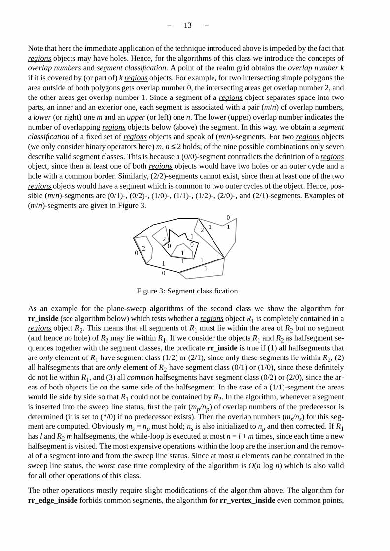
Note that here the immediate application of the technique introduced above is impeded by the fact thatregions objects may have holes. Hence, for the algorithms of this class we introduce the concepts ofoverlap numbers and segment classification. A point of the realm grid obtains the overlap number kif it is covered by (or part of) k regions objects. For example, for two intersecting simple polygons thearea outside of both polygons gets overlap number 0, the intersecting areas get overlap number 2, andthe other areas get overlap number 1. Since a segment of a regions object separates space into twoparts, an inner and an exterior one, each segment is associated with a pair (m/n) of overlap numbers,a lower (or right) one m and an upper (or left) one n. The lower (upper) overlap number indicates thenumber of overlapping regions objects below (above) the segment. In this way, we obtain a segmentclassification of a fixed set of regions objects and speak of (m/n)-segments. For two regions objects(we only consider binary operators here) m, n ≤ 2 holds; of the nine possible combinations only sevendescribe valid segment classes. This is because a (0/0)-segment contradicts the definition of a regionsobject, since then at least one of both regions objects would have two holes or an outer cycle and ahole with a common border. Similarly, (2/2)-segments cannot exist, since then at least one of the tworegions objects would have a segment which is common to two outer cycles of the object. Hence, pos-sible (m/n)-segments are (0/1)-, (0/2)-, (1/0)-, (1/1)-, (1/2)-, (2/0)-, and (2/1)-segments. Examples of(m/n)-segments are given in Figure 3.
As an example for the plane-sweep algorithms of the second class we show the algorithm forrr_inside (see algorithm below) which tests whether a regions object R1 is completely contained in aregions object R2. This means that all segments of R1 must lie within the area of R2 but no segment(and hence no hole) of R2 may lie within R1. If we consider the objects R1 and R2 as halfsegment se-quences together with the segment classes, the predicate rr_inside is true if (1) all halfsegments thatare only element of R1 have segment class (1/2) or (2/1), since only these segments lie within R2, (2)all halfsegments that are only element of R2 have segment class (0/1) or (1/0), since these definitelydo not lie within R1, and (3) all common halfsegments have segment class (0/2) or (2/0), since the ar-eas of both objects lie on the same side of the halfsegment. In the case of a (1/1)-segment the areaswould lie side by side so that R1 could not be contained by R2. In the algorithm, whenever a segmentis inserted into the sweep line status, first the pair (mp/np) of overlap numbers of the predecessor isdetermined (it is set to (*/0) if no predecessor exists). Then the overlap numbers (ms/ns) for this seg-ment are computed. Obviously ms = np must hold; ns is also initialized to np and then corrected. If R1has l and R2 m halfsegments, the while-loop is executed at most n = l + m times, since each time a newhalfsegment is visited. The most expensive operations within the loop are the insertion and the remov-al of a segment into and from the sweep line status. Since at most n elements can be contained in thesweep line status, the worst case time complexity of the algorithm is O(n log n) which is also validfor all other operations of this class.
The other operations mostly require slight modifications of the algorithm above. The algorithm forrr_edge_inside forbids common segments, the algorithm for rr_vertex_inside even common points,
2
1
0
02
20
0
1
11
1
11
01
Figure 3: Segment classification
− 14 −
a problem which to treat is a little bit more complicated. The operation rr_area_disjoint yields trueif both objects have no common areas and only allows (0/1)-, (1/0)-, and (1/1)-segments. The opera-tion rr_edge_disjoint additionally forbids common segments (no (1/1)-segments) and rr_disjointeven common points which needs a little bit more effort. The operation rr_adjacent which checksthe neighbourhood of two regions objects is equal to rr_area_disjoint but additionally requires theexistence of at least one (1/1)-segment. The operation rr_meets which checks whether two regionsobjects meet in a point is equal to rr_edge_disjoint but additionally requires the existence of at leastone common point. The operation rr_intersects is true if two regions objects have a common areawhich means that there exist some segments of segment class (0/2), (1/2), (2/0), or (2/1). The follow-ing three operations produce a new regions object. The intersection of two regions objects (operationrr_intersection) implies the search for all segments with segment classification (0/2), (1/2), (2/0), and(2/1). For the union of two regions objects (operation rr_union) all (0/1)-, (1/0)-, (0/2)-, and (2/0)-segments are collected. The computation of the difference of two regions objects R1 and R2 (operationrr_minus) requires all (0/1)- and (1/0)-segments of R1, all (1/2)- and (2/1)-segments of R2, and allcommon (1/1)-segments. The operation rr_encloses yields true for two regions objects R1 and R2 ifeach face and hence each segment of R2 is contained in a hole of R1. Note that this condition does notmean that R1 and R2 are area-disjoint, since it is possible that another face of R1 lies within R2. Herea method is used which gives the overlap numbers a different interpretation: We do not consider theoverlapping of object areas but the overlapping of the single cycle areas of an object. In this way, theexterior of R1 gets the number 0, the area of a face of R1 the number 1, and a hole the number 2. If ahole of R1 contains another face of the same object, this face gets the number 3 and a hole of this facethe number 4, etc. If we compute such a segment classification for R1, then R1 encloses R2 if all seg-ments of R2 lie on a level with even overlap number (greater than 0).
if ((object = first) or (object = both)) and(InsideAbove ∈ get_attr(R1))then ns := ns + 1else ns := ns − 1
end-if;if ((object = second) or (object = both)) and
(InsideAbove ∈ get_attr(R2))then ns := ns + 1else ns := ns − 1
end-if;S := set_attr(S, (ms/ns));if object = first then
inside := ((ms/ns) ∈ {(1/2), (2/1)})else if object = second then
inside := ((ms/ns) ∉ {(1/2), (2/1)})else
inside := ((ms/ns) ∈ {(0/2), (2/0)})end-if;
end-if;rr_select_next(R1, R2, object, status);
end-while;return inside;
end rr_inside.
algorithm rr_insideinput: Two regions objects R1 and R2output:true, if R1 lies within R2
false, otherwisebegin
S := new_sweep();inside := true;rr_select_first(R1, R2, object, status);while (status ≠ end_of_first) and inside do
if (object = first) or (object = both)then h := get_hs(R1); (* Let h = (s, d) . *)else h := get_hs(R2); (* Let h = (s, d) . *)
end-if;if d = right then
S := del_right(S, s);else
S := add_left(S, s);if not pred_exists(S)
then mp/np := */0else mp/np := get_pred_attr(S)
end-if;ms := np;ns := np;
− 15 −
4.3 Graph Algorithms
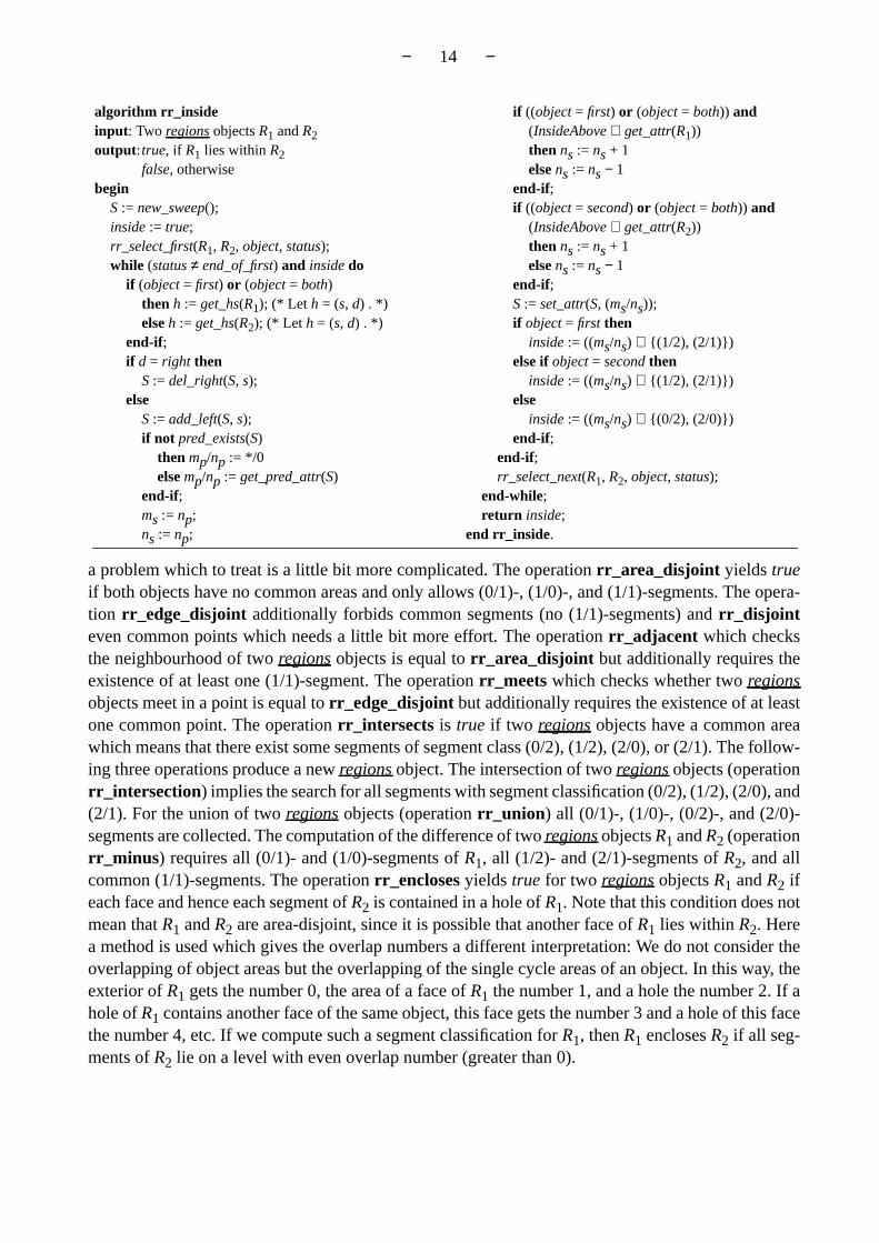
A realm can be interpreted as a spatially embedded planar graph [GüS93a]. Hence, alines or aregionsobject defined over such a realm can also be regarded as a planar graphG = (V, E) where the vertexsetV is the set of all end points of the segments and the edge setE is the set of all segments of theobject. Note that such anembedded planar graph represents not only the usual incidence relationshipsbetween nodes and edges, but also theneighbourhood relationship among segments incident to thesame node. This graph-theoretic view offers two primitive operations, illustrated in Figure 4, that arecrucial for the algorithms discussed in this section: For a given halfsegment, (i) find its two neighboursincident to the same node w.r.t. the counter-clockwise order, and (ii) find the “partner halfsegment”representing the same segment (which is equivalent to following an edge of the graph).
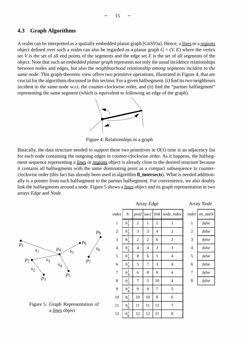
Basically, the data structure needed to support these two primitives inO(1) time is an adjacency listfor each node containing the outgoing edges in counter-clockwise order. As it happens, the halfseg-ment sequence representing alines or regions object is already close to the desired structure becauseit contains all halfsegments with the same dominating point as a compact subsequence in counter-clockwise order (this fact has already been used in algorithmll_intersects). What is needed addition-ally is a pointer from each halfsegment to the partner halfsegment. For convenience, we also doublylink the halfsegments around a node. Figure 5 shows alines object and its graph representation in twoarraysEdge and Node.
Figure 4: Relationships in a graph
Array Edge
index h pred succ link node_index
1 1 1 5 1
2 3 3 4 2
3 2 2 6 2
4 4 4 2 3
5 8 6 1 4
6 5 7 3 4
7 6 8 9 4
8 7 5 10 4
9 9 9 7 5
10 10 10 8 6
11 11 11 12 7
12 12 12 11 8
h1l
h2l
h3l
h2r
h1r
h3r
h4l
h5l
h4r
h5r
h6l
h6r
Array Node
index on_stack
1 false
2 false
3 false
4 false
5 false
6 false
7 false
8 false
p1
p2
p3
p4
p6
p5
p7
p8
s1
s3
s2
s5
s4
s6
Figure 5: Graph Representation ofa lines object
− 16 −
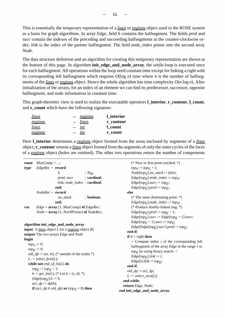
This is essentially the temporary representation of a lines or regions object used in the ROSE systemas a basis for graph algorithms. In array Edge, field h contains the halfsegment. The fields pred andsucc contain the indexes of the preceding and succeeding halfsegments in the counter-clockwise or-der; link is the index of the partner halfsegment. The field node_index points into the second arrayNode.
The data structure definition and an algorithm for creating this temporary representation are shown atthe bottom of this page. In algorithm init_edge_and_node_array, the while-loop is executed oncefor each halfsegment. All operations within the loop need constant time except for linking a right withits corresponding left halfsegment which requires O(log n) time where n is the number of halfseg-ments of the lines or regions object. Hence the whole algorithm has time complexity O(n log n). Afterinitialization of the arrays, for an index of an element we can find its predecessor, successor, oppositehalfsegment, and node information in constant time.
This graph-theoretic view is used to realize the executable operators l_interior, r_contour, l_count,and r_count which have the following signature:
lines → regions l_interiorregions → lines r_contourlines → int l_countregions → int r_count
Here l_interior determines a regions object formed from the areas enclosed by segments of a linesobject, r_contour returns a lines object formed from the segments of only the outer cycles of the facesof a regions object (holes are omitted). The other two operations return the number of components
(* New or first point reached. *)topV := topV + 1;Node[topV].on_stack := false;Edge[topE].node_index := topV;Edge[topE].succ := topE;Edge[topE].pred := topE;
else(* The same dominating point. *)Edge[topE].node_index := topV;(* Produce doubly-linked ring. *)Edge[topE].pred := topE − 1;Edge[topE].succ := Edge[topE − 1].succ;Edge[topE − 1].succ := topE;Edge[Edge[topE].succ].pred := topE;
end-if;if d = right then
< Compute index i of the corresponding lefthalfsegment of the array Edge in the range 1 totopE by using binary search. >Edge[topE].link := i;Edge[i].link := topE;
end-if;old_dp := act_dp;L := select_next(L);
end-while;return Edge, Node;
end init_edge_and_node_array.
const MaxComp = ...;type EdgeRec = record
h : HN;pred, succ : cardinal;link, node_index : cardinal;
end;NodeRec = record
on_stack : boolean;end;
var Edge = array [1..MaxComp] of EdgeRec;Node = array [1..NoOfPoints] of NodeRec;
algorithm init_edge_and_node_arrayinput: A lines object L (or a regions object R)output:The two arrays Edge and Nodebegin
topV := 0;topE := 0;old_dp := (m, m); (* outside of the realm *)L := select_first(L);while not end_of_hs(L) do
topE := topE + 1;h := get_hs(L); (* Let h = (s, d). *)Edge[topE].h := h;act_dp := dp(h);if (act_dp ≠ old_dp) or (topV = 0) then
− 17 −
which is the number of blocks (connected components) for alines object and the number of faces fora regions object. As an example, we show the algorithm forr_contour.
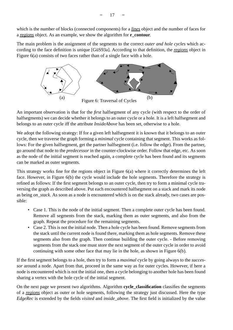
The main problem is the assignment of the segments to the correctouter and hole cycles which ac-cording to the face definition is unique [GüS93a]. According to that definition, theregions object inFigure 6(a) consists of two faces rather than of a single face with a hole.
An important observation is that for thefirst halfsegment of any cycle (with respect to the order ofhalfsegments) we can decide whether it belongs to an outer cycle or a hole. It is a left halfsegment andbelongs to an outer cycle iff the attributeInsideAbove has been set, otherwise to a hole.
We adopt the following strategy: If for a given left halfsegment it is known that it belongs to an outercycle, then we traverse the graph forming aminimal cycle containing that segment. This works as fol-lows: For the given halfsegment, get the partner halfsegment (i.e. follow the edge). From the partner,go around that node to thepredecessor in the counter-clockwise order. Follow that edge, etc. As soonas the node of the initial segment is reached again, a complete cycle has been found and its segmentscan be marked as outer segments.
This strategy works fine for the regions object in Figure 6(a) where it correctly determines the leftface. However, in Figure 6(b) the cycle would include the hole segments. Therefore the strategy isrefined as follows: If the first segment belongs to an outer cycle, then try to form a minimal cycle tra-versing the graph as described above. Put each encountered halfsegment on a stack and mark its nodeas beingon_stack. As soon as a node is encountered which is on the stack already, two cases are pos-sible:
• Case 1. This is the node of the initial segment. Then a complete outer cycle has been found.Remove all segments from the stack, marking them as outer segments, and also from thegraph. Repeat the procedure for the remaining segments.
• Case 2. This is not the initial node. Then a hole cycle has been found. Remove segments fromthe stack until the current node is found there, marking them as hole segments. Remove thesesegments also from the graph. Then continue building the outer cycle. - Before removingsegments from the stack one must store the next segment of the outer cycle in order to avoidcontinuing with some other face that may lie in the hole, as shown in Figure 6(b).
If the first segment belongs to a hole, then try to form amaximal cycle by going always to thesucces-sor around a node. Apart from that, proceed in the same way as for outer cycles. However, if here anode is encountered which is not the initial one, then a cycle belonging to another hole has been foundsharing a vertex with the hole cycle of the initial segment.
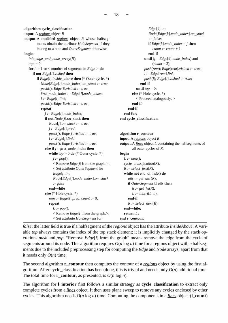
On the next page we present two algorithms. Algorithmcycle_classification classifies the segmentsof a regions object as outer or hole segments, following the strategy just discussed. Here the typeEdgeRec is extended by the fieldsvisited andinside_above. The first field is initialized by the value
Figure 6: Traversal of Cycles(a) (b)
− 18 −
false; the latter field is true if a halfsegment of the regions object has the attribute InsideAbove. A vari-able top always contains the index of the top stack element; it is implicitly changed by the stack op-erations push and pop. “Remove Edge[j] from the graph” means remove the edge from the cycle ofsegments around its node. This algorithm requires O(n log n) time for a regions object with n halfseg-ments due to the included preprocessing step for computing the Edge and Node arrays; apart from thatit needs only O(n) time.
The second algorithm r_contour then computes the contour of a regions object by using the first al-gorithm. After cycle_classification has been done, this is trivial and needs only O(n) additional time.The total time for r_contour, as presented, is O(n log n).
The algorithm for l_interior first follows a similar strategy as cycle_classification to extract onlycomplete cycles from a lines object. It then uses plane sweep to remove any cycles enclosed by othercycles. This algorithm needs O(n log n) time. Computing the components in a lines object (l_count)
Edge[k]. >;Node[Edge[k].node_index].on_stack := false;if Edge[k].node_index = j then
count := count + 1end-if
until (j = Edge[k].node_index) and(count = 2);
push(rem); Edge[rem].visited := true;l := Edge[rem].link;push(l); Edge[l].visited := true;
end-ifuntil top = 0;
else (* Hole cycle. *)< Proceed analogously. >
end-ifend-if
end-for;endcycle_classification.
algorithm r_contourinput : A regions object Routput:A lines object L containing the halfsegments of
all outer cycles of R.begin
L := new();cycle_classification(R);R := select_first(R);while not end_of_hs(R) do
attr := get_attr(R);if OuterSegment ∈ attr then
h := get_hs(R);L := insert(L, h);
end-if;R := select_next(R);
end-while;return L;
end r_contour.
algorithm cycle_classificationinput : A regions object Routput:A modified regions object R whose halfseg-
ments obtain the attribute HoleSegment if theybelong to a hole and OuterSegment otherwise.
begininit_edge_and_node_array(R);top := 0;for i := 1 to < number of segments in Edge > do
if not Edge[i].visited thenif Edge[i].inside_above then (* Outer cycle. *)
Node[Edge[i].node_index].on_stack := true;push(i); Edge[i].visited := true;first_node_index := Edge[i].node_index;l := Edge[i].link;push(l); Edge[l].visited := true;repeat
j := Edge[l].node_index;if not Node[j].on_stack then
Node[j].on_stack := true;j := Edge[l].pred;push(j); Edge[j].visited := true;l := Edge[j].link;push(l); Edge[l].visited := true;
elseif j = first_node_index thenwhile top > 0 do (* Outer cycle. *)
j := pop();< Remove Edge[j] from the graph. >;< Set attribute OuterSegment forEdge[j]. >;Node[Edge[j].node_index].on_stack:= false
end-whileelse (* Hole cycle. *)
rem := Edge[l].pred; count := 0;repeat
k := pop();< Remove Edge[j] from the graph.>;< Set attribute HoleSegment for
− 19 −
can be done by a simple depth-first traversal [AhHU83]. Determining the number of components (fac-es) in a regions object is also a by-product of cycle classification. The last two algorithms require O(n)time once the graph representation has been constructed.
4.4 Special Algorithms
The diameter operator of the ROSE algebra determines the maximal extent of an object, that is, themaximal distance between any two vertices. The implementation of the corresponding three execut-able operators p_diameter, l_diameter, and r_diameter uses special algorithms different from thethree techniques mentioned before. The computation of all distances between any two points of anobject is too time-consuming. To reduce the number of elements, we determine the convex hull of theobject, since the diameter of the convex hull is equal to the diameter of the whole object [PrS85]. Analgorithm which calculates the convex hull of the point set of a simple polygon in linear time can befound in [Me84]. An algorithm which computes the diameter of a convex polygon in linear time isshown in [PrS85]. The combination of these two algorithms is used in the ROSE system to realize thethree diameter operations in O(n) time for an object with n points or halfsegments.
5 Implementation
In this section we discuss in more detail the actual representation of ROSE objects and some differ-ences between the conceptual view of algorithms, as presented above, and the actual procedures inthe system. On the next page, the representation of a regions object is shown (for points and lines ob-jects it is similar). A regions object is given as (a pointer to) a record whose last component is an arrayelem; one can dynamically allocate storage to represent regions objects of any desired size. The arrayserves as a storage pool for three different kinds of nodes representing halfsegments, faces, or holes,respectively. Halfsegments are organized in an AVL-tree to allow for updates in O(log n) time; addi-tional pointers connect all halfsegments within the object, within a face, and within a cycle (outer cy-cle or hole cycle) into linked lists ordered in halfsegment order. Additionally all faces, and for eachface its holes, are linked. Hence the complete structure of a regions object is explicitly representedand access operations are offered (in the module hiding this representation) to perform all kinds ofscans in linear time. Furthermore, bounding boxes are stored for the object, each face, and each hole.The record contains general information about the object such as the root segment of the AVL-tree,fields for perimeter, diameter and area; the attr field tells which of these values have already beencomputed for this particular object.
In Section 4.3, we have described the graph algorithms from a conceptual point of view. What reallyhappens is that the graph structure is analyzed at the time of closing an object, that is, after all seg-ments have been inserted. More precisely, the construction of a regions object consists of the follow-ing steps:
• Allocate storage, insert n halfsegments into the AVL-tree.
To close the object:• Perform an inorder traversal of the tree to link all halfsegments of the object; compute the
bounding box.• Use plane sweep to compute InsideAbove attributes (sketched in Section 4.2).• Use algorithm cycle_classification (including init_edge_and_node_array) to attach a

− 20 −
unique cycle number to each segment.• Use a second plane sweep (a variant of the previous one) to determine for each hole segment
the cycle number of the outer cycle of its surrounding face.• In a final scan of the complete list of segments, link all segments within faces and cycles (this
is possible since each segment has now an associated cycle number and face number) andcompute the remaining information such as bounding boxes, links of faces and holes, etc.
Clearly the whole construction takes no more than O(n log n) time and O(n) space. An analogous strat-egy is used for the more simple lines and points objects. Because all this information is now explicitlyavailable in the data structures, the algorithms and running times for some operations change: allno_of_components algorithms perform a simple lookup in O(1) time. The algorithm for r_contoursimply scans the list of faces and for each face the list of segments of its outer cycle which requiresonly O(k log k) time (where k is the size of the result object). For operators computing diameter,length, area and perimeter, only the first call takes O(n) time; the value is then stored with the object
FROM Primitives IMPORT
(* type *) BBOX, HALFSEGMENT, POINT, SEGMENT;
TYPE OBJATTRIBS = (Closed, Perimeter, Diameter, Area); ATTRIBSET = SET OF OBJATTRIBS; COMPATTRIBS = (InsideUp, HoleSegment); COMPSET = SET OF COMPATTRIBS; FIELDTYPE = (HalfsegField, FaceField, HoleField); SELECTTYPE = (RegionsSelected, FaceSelected, CycleSelected);
REGIONSELEM = RECORD CASE kind : FIELDTYPE OF HalfsegField: h : HALFSEGMENT; (* Key-element. *) attrib : COMPSET; (* Element status.*) left : CARDINAL; (* AVL-tree. *) right : CARDINAL; height : CARDINAL; next_in_regions : CARDINAL; (* In order lists.*) next_in_face : CARDINAL; next_in_cycle : CARDINAL; | FaceField: face_bbox : BBOX; (* Face bounding box. *) first_in_face : CARDINAL; (* First halfsegment. *) last_in_face : CARDINAL; (* (Help pointer.) *) last_in_cycle : CARDINAL; (* (Help pointer.) *) first_hole : CARDINAL; (* First hole in face. *) last_hole : CARDINAL; (* (Help pointer.) *) next_face : CARDINAL; (* Face list. *) | ELSE hole_bbox : BBOX; (* Hole bounding. *) first_in_hole : CARDINAL; (* First Halfsegment. *) last_in_hole : CARDINAL; (* (Help pointer.) *) next_hole : CARDINAL; (* Hole list. *) END; END;
REGIONS = POINTER TO RECORD attr : ATTRIBSET; (* The object’s status. *) perimeter : REAL; (* Length of Segments. *) diameter : REAL; (* Diameter. *) area : REAL; (* Area of object. *) bbox : BBOX; (* Bounding box. *) count : CARDINAL; (* Number of faces. *) holes : CARDINAL; (* Number of holes. *) free : CARDINAL; (* Number of free fields. *) first_idx : CARDINAL; (* Idx of smallest halfseg. *) face_idx : CARDINAL; (* Idx of first face. *) root_idx : CARDINAL; (* Idx of root of AVL-tree. *) act_idx : CARDINAL; (* Idx of selected halfseg. *) act_face : CARDINAL; (* Idx of selected face. *) sel_kind : SELECTTYPE; (* Kind of traversal. *) max_idx : CARDINAL; (* Idx of largest half-field. *) act_hole : CARDINAL; (* Idx of selected hole. *) elem : ARRAY [1..MaxInRegions] OF REGIONSELEM END;

− 21 −
so that subsequent calls are lookups inO(1) time. Further differences between the algorithms de-scribed above and the actual procedures result from:
• Use of filter techniques. Most operations first compare bounding boxes of objects, some in asecond step also component bounding boxes, in order to avoid running the more expensivealgorithms on the actual halfsegments, whenever possible. Such strategies are well-known(e.g. [OrM88, Gü94]).
• Estimating the size of the result is necessary in all operations constructing new objects to al-locate the appropriate amount of storage for them.
For further details, we recommend the study of [Ri95].
6 Conclusions
We have described the implementation of a large part of a spatial algebra for database systems - thatis, the almost complete implementation of the first three groups of operators of the ROSE algebra(only thedist operator is missing) which deal with “atomic” objects (whereas the fourth group ma-nipulates set of database objects). Use of high-level primitives has made it possible to describe a rel-atively large number of algorithms in compact, precise notation. We are not aware of any similar work- treating a whole algebra by giving precise algorithms including analysis of their complexity.
The fact that ROSE objects are realm-based has led to relatively simple, efficient, and numericallyrobust algorithms. All manipulations of objects are discrete (entirely based on integer arithmetics);real numbers occur only to describe properties such as length or area of objects. A crucial concept isthe use of ordered halfsegment sequences as a base representation of objects. Manipulation of suchsequences in parallel traversal or plane sweep implements most operations efficiently. On the otherhand, we have also shown how the structure of objects (faces, holes, etc.) can be determined by graphalgorithms and be represented in the data structures.
The ROSE system is available for study or use, currently in the form of a stand-alone Modula-2 library[Ri95]. It is in principle suitable for use in database systems since all objects have compact represen-tations. However, for a serious integration it is necessary to solve the problem of managing very largeROSE objects in a way that is compatible with the DBMS object and storage management. We arecurrently working on the definition and implementation of a general “algebra interface” between anexternal implementation of a system of data types and a database system. The ROSE algebra will bemade available under such an interface and integrated into the Gral system [Gü89, BeG92]. In thisapproach, it is only necessary to replace the array components “at the end” of object representationsby identifiers of so-called “database arrays” which behave exactly like ordinary arrays but have theirown page sequences and buffer management and interact properly with DBMS transaction manage-ment. This is a straightforward, technical modification of the ROSE algebra; algorithms remain un-changed.
Another aspect of integration into a database system is the connection to the underlying realms, in par-ticular the propagation of updates from the realm to ROSE objects in a database [GüS93a]. Our realmimplementation is almost completed. All these integration aspects will be described in a forthcomingpaper.

− 22 −
Appendix
The structure of this table is explained in Section 2. In column “time complexity” (TC), n denotes thetotal size of the operand(s), m the size of the regions operand (only used if there is just one), and k thesize of the result object.
Descriptive Operator Executable Operator PT PS G TC
geo × geo → bool = pp_equal, ll_equal, rr_equal x O(n)
≠ pp_unequal, ll_unequal,rr_unequal
x O(n)
disjoint pp_disjoint, ll_disjoint x O(n)
rr_disjoint x O(n log n)
geo × regions → bool inside pr_inside, lr_inside x O(n log m)
rr_inside x O(n log n)
regions × regions → bool area_disjoint rr_area_disjoint x O(n log n)
edge_disjoint rr_edge_disjoint x O(n log n)
edge_inside rr_edge_inside x O(n log n)
vertex_inside rr_vertex_inside x O(n log n)
ext1 × ext2 → bool intersects ll_intersects x O(n)
lr_intersects, rl_intersects x O(n log m)
rr_intersects x O(n log n)
meets ll_meets x O(n)
lr_meets, rl_meets x O(n log m)
rr_meets x O(n log n)
border_in_common ll_border_in_common,lr_border_in_common,rl_border_in_common,rr_border_in_common
x O(n)
area × area → bool adjacent rr_adjacent x O(n log n)
encloses rr_encloses x O(n log n)
points × ext → bool on_border_of pl_on_border_of,pr_on_border_of
x O(n)
points × points → points intersection pp_intersection x O(n + k log k)
lines × lines → points intersection ll_intersection x O(n + k log k)
regions × regions → regions intersection rr_intersection x O(n log n)
regions × lines → lines intersection rl_intersection x O(n log m +k log k)
geo × geo → geo plus pp_plus, ll_plus x O(n + k log k)
rr_plus x O(n log n)

− 23 −
References
[AhHU83] Aho, A.V., J.E. Hopcroft, and J.D. Ullman,Data Structures and Algorithms. Addison-Wesley, Reading,Massachusetts, 1983.
[BeG92] Becker, L., and R.H. Güting, Rule-Based Optimization and Query Processing in an ExtensibleGeometric Database System.ACM Transactions on Database Systems 17 (1992), 247-303.
[GrY86] Greene, D., and F. Yao, Finite-Resolution Computational Geometry. Proc. 27th IEEE Symp. onFoundations of Computer Science, 1986, 143-152.
[Gü89] Güting, R.H., Gral: An Extensible Relational Database System for Geometric Applications. Proc. of the15th Intl. Conf. on Very Large Databases (Amsterdam, The Netherlands), 1989, 33-44.
[Gü93] Güting, R.H., Second-Order Signature: A Tool for Specifying Data Models, Query Processing, andOptimization. Proc. ACM SIGMOD Conf. (Washington, USA), 1993, 277-286.
[Gü94] Güting, R.H., An Introduction to Spatial Database Systems.VLDB Journal 3, 4 (1994) (Special Issue onSpatial Database Systems), 357-399.
[GüS93a] Güting, R.H., and M. Schneider, Realms: A Foundation for Spatial Data Types in Database Systems.Proc. of the 3rd Intl. Symposium on Large Spatial Databases (Singapore), 1993, 14-35.
[GüS93b] Güting, R.H., and M. Schneider, Realm-Based Spatial Data Types : The ROSE Algebra. FernuniversitätHagen, Informatik-Report 141, 1993. To appear in theVLDB Journal.
[KaM85] Karlsson, R.G., and J.I. Munro, Proximity on a Grid.Proc. of the 2nd Symp. on Theoretical Aspects ofComputer Science, Springer-Verlag, LNCS 182, 1985, 187-196.
[KaO88a] Karlsson, R.G., and M.H. Overmars, Scanline Algorithms on a Grid.BIT 28 (1988), 227-241.
geo × geo → geo minus pp_minus, ll_minus x O(n + k log k)
rr_minus x O(n log n)
ext1 × ext2 → lines common_border ll_common_border,lr_common_border,rl_common_border,rr_common_border
x O(n + k log k)
ext → points vertices l_vertices, r_vertices x O(n + k log k)
regions → lines contour r_contour x O(n log n) /O(k log k)
lines → regions interior l_interior x O(n log n)
geo → int no_of_components p_no_of_components x O(n) / O(1)
l_no_of_components,r_no_of_components
x O(n log n) /O(1)
geo1 × geo2 → real dist pp_dist, pl_dist, pr_dist, lp_dist,ll_dist, lr_dist, rp_dist, rl_dist,rr_dist
geo → real diameter p_diameter, l_diameter,r_diameter
special algo-rithm
O(n) / O(1)
lines → real length l_length x O(n) / O(1)
regions → real area r_area x O(n) / O(1)
perimeter r_perimeter x O(n) / O(1)
Descriptive Operator Executable Operator PT PS G TC
− 24 −
[KaO88b] Karlsson, R.G., and M.H. Overmars, Normalized Divide-and-Conquer: A Scaling Technique for SolvingMulti-Dimensional Problems.Information Processing Letters 26 (1988), 307-312.
[KeK81] Keil, J.M., and D.G. Kirkpatrick, Computational Geometry on Integer Grids.Proc. of the 19th AnnualAllerton Conference on Communication, Control, and Computing, 1981, 41-50.
[Kl83] Klaeren, H.A.,Algebraische Spezifikation. Springer Verlag, Berlin, 1983.
[Me84] Mehlhorn, K., Data Structures and Algorithms 3: Multidimensional Searching and ComputationalGeometry. Springer Verlag, 1984.
[Mü85] Müller, H., Rastered Point Location.Proc. Workshop on Graphtheoretic Concepts in Computer Science,Trauner Verlag, 1985, 281-293.
[OrM88] Orenstein, J., and F. Manola, PROBE Spatial Data Modeling and Query Processing in an ImageDatabase Application.IEEE Trans. on Software Engineering 14 (1988), 611-629.
[Ov88a] Overmars, M.H., Efficient Data Structures for Range Searching on a Grid.Journal of Algorithms 9(1988), 254-275.
[Ov88b] Overmars, M.H., New Algorithms for Computer Graphics.Advances in Computer Graphics,Eurographics Seminars, Springer Verlag, 1988, 3-19.
[Ov88c] Overmars, M.H., Computational Geometry on a Grid: An Overview. Theoretical Foundations forComputer Graphics and CAD, Springer Verlag, 1988, 167-184.
[PrS85] Preparata F.P., and M.I. Shamos,Computational Geometry. Springer Verlag, 1985.
[Ri95] de Ridder, T., The ROSE System. Modula-2 Program System (Source Code). Fernuniversität Hagen,Praktische Informatik IV, Software Report 1, 1995. Available as a LaTeX file for printing and/or as acompressed collection of ASCII files.
[Ya92] Yao F.F., Computational Geometry. Algorithms and Complexity. Handbook of Theoretical ComputerScience, vol. A, Elsevier Science Publishers B.V., 1992, 343-389.