International Journal on Digital Libraries (2005)DOI 10.1007/s00799-005-0118-z

REGULAR PAPER

Shu-Yuen D. Yao · Cyrus Shahabi · Roger Zimmermann

BroadScale: Efficient scaling of heterogeneous storage systems

Published online: 25 October 2005c© Springer-Verlag 2005

Abstract Scalable storage architectures enable digital li-braries and archives for the addition or removal of storagedevices to increase storage capacity and bandwidth or retireolder devices. Past work in this area have mainly focused onstatically scaling homogeneous storage devices. However,heterogeneous devices are quickly being adopted for stor-age scaling since they are usually faster, larger, more widelyavailable, and more cost-effective. We propose BroadScale,an algorithm based on Random Disk Labeling, to dynam-ically scale heterogeneous storage systems by distributingdata objects according to their device weights. Assuminga random placement of objects across a group of hetero-geneous storage devices, our optimization objectives whenscaling are to ensure a uniform distribution of objects, re-distribute a minimum number of objects, and maintain fastdata access with low computational complexity. We showthrough experimentation that BroadScale achieves these re-quirements when scaling heterogeneous storage.

Keywords Scalable storage systems · Random dataplacement · Load balancing · Heterogeneous disk scaling

1 Introduction

Computer applications typically require ever-increasingstorage capacity to meet the demands of their expandingdata sets. Because storage requirements oftentimes exhibitvarying growth rates, current storage systems may not re-serve a sufficient amount of excess space for future growth.Meanwhile, large up-front costs should not be incurred fora storage system that might only be fully utilized in the dis-tant future. Therefore, a storage system that accommodatesincremental growth would have major cost benefits. Incre-mental growth translates into a highly scalable storage sys-tem where the amount of overall storage space and through-

S.-Y. D. Yao (B) · C. Shahabi · R. ZimmermannUniversity of Southern California, Computer Science Department,Los Angeles, CA 90089E-mail: didiyao@usc.edu

put can dynamically expand according to the growth rate ofits content data and/or application performance needs.

Our proposed scalable storage algorithms are general-ized solutions for mapping a set of data objects to a group ofstorage units. Furthermore, the objects are striped indepen-dently of each other across all of the storage units for load-balancing purposes, that is, any object can be accessed withalmost equal probability. This group of storage units has thequality that more units can be either added or removed, inwhich case the striped objects need to be redistributed tomaintain a balanced load.

Scientific digital archives, distributed file systems, Webproxy servers, and continuous media (CM) servers are eachexamples of storage systems found in digital libraries. Thesesystems experience growing data content and can benefitfrom a generalized and scalable storage solution. The Scien-tific Archive Management (SAM) system developed at thePacific Northwest National Laboratory stores a very large,increasing amount of data generated from scientific experi-ments [21]. SAM relies on metadata and a virtual file sys-tem on its storage farms to allow scientists to store theirdata without worrying about the underlying data localityeven when data is relocated due to system scale-up. Lustre1

is an example of a highly scalable cluster file system thatcould benefit from efficient data redistribution techniqueswhen adding more cluster nodes. A low-cost scaling tech-nique is crucial for Lustre since it aims to scale up to tensof thousands of nodes. Distributed CM servers provide real-time access to libraries of digital media where the media filesare declustered across a large set of disks. We assume CMservers in our discussions and use the terms “disk” and “fileblock” (i.e., of a file object) in place of “storage unit” and“data object,” respectively, throughout this paper. Finally,other familiar examples of exponentially growing data storeswith high-scalability requirements are the Google2 search

1 http://www.lustre.org/2 http://www.google.com/

S.-Y. D. Yao et al.

engine and the Internet Archive3 library of digitized histori-cal collections.

Our technique to achieve a highly scalable CM serverbegins with the placement of data on storage devices such asmagnetic disk drives [11, 17]. More specifically, we breakCM files (e.g., video or audio) into individual fixed-sizeblocks and apply a random placement [12] of these blocksacross a group of homogeneous disks. Since any block canbe accessed with an almost equal probability the randomstriping scheme allows the disks to be load balanced wheretheir aggregate bandwidth and capacity (e.g., in bits/secondand bytes, respectively) are maximized when accessing CMfiles. We actually use a pseudo-randomized placement of fileobject blocks, as in [6, 17], so that blocks have roughly equalprobabilities of residing on each disk. With pseudo-randomdistribution, blocks are placed onto disks in a random, butreproducible, sequence.

The placement of block i is determined by its signatureXi , which is simply an unsigned integer computed from apseudo-random number generator, p_r . p_r must producerepeatable sequences for a given seed. One way to derivethe seed is from (StrToL4(filename) + i), which is used toinitialize the pseudo-random function to compute Xi .

The storage system of a CM server requires that disksbe scaled (i.e., added or removed) in which case the stripedobjects need to be redistributed to maintain a balanced load.Disks can be added to the system to increase overall band-width and capacity or removed due to failure or space con-servation. We use the notion of disk group as a group of disksthat is added or removed during a scaling operation. With-out loss of generality, a scaling operation on a storage systemwith D disks either adds or removes one disk group. Scalingup will increase the total number of disks and will require afraction of all blocks to be moved onto the added disks in or-der to maintain load balancing across disks. Likewise, whenscaling down, all blocks on a removed disk should be ran-domly distributed across remaining disks to maintain loadbalancing. These block moves are the minimum needed tomaintain an even load. Note that disk removals are only usedfor scaling down a system and conserving space. A disk re-moval and a disk failure are different in that data must bemoved off of a disk before it is removed. With disk failures,data cannot be moved off a priori so a fault tolerance tech-nique such as RAID-5 can be used in conjunction with RDLto prevent data loss. Our work is orthogonal to fault toler-ance techniques such as RAID-5 since, in our scenario, eachdisk represents a logical storage unit and can potentially bea RAID device itself. Thus, our focus in this paper is on theissue of storage scalability.

We have previously developed the Random Disk Label-ing algorithm to assign blocks to homogeneous disks usingblock signatures [23]. However, a homogeneous disk groupmay not be available at the time of scaling due to advance-ments in storage technology [7]. Thus, larger, faster, andmore cost-effective heterogeneous disks must be used when

3 http://www.archive.org/4 StrToL is a C function that converts a string into a long integer.

scaling to increase the overall bandwidth and capacity char-acteristics of the storage system. The number of blocks oneach disk should be proportional to both these characteris-tics. Load balancing according to just bandwidth may over-flow some disks earlier than others since a disk with twicethe bandwidth may not necessarily have twice the capacity.

In this paper, we propose the BroadScale algorithm forthe disk assignment and scaling of heterogeneous disks. Inaddition to a block signature, a disk weight is assigned toeach disk depending on its capacity and bandwidth. We willshow that the system is load balanced after blocks are allo-cated according to both block signatures and disk weights.

As disks are added to and removed from the system, thelocation of a block may change. Our objective of course is toquickly compute the current location of a block, regardlessof how many scaling operations have been performed. More-over, we must ensure an even load on the disks and minimalblock movement during a scaling operation. We summarizethe requirements more clearly as follows.

Requirement 1 (even load): If there are B blocks storedon D disks, maintain the load so that the expected numberof blocks on disk d is approximately wd∑D−1

j=0 w j× B where wd

is the weight of disk d .Requirement 2 (minimal data movement): During the ad-

dition of n disks on a system with D disks storing B blocks,

the expected number of block moves is∑D+n−1

j=D w j∑D+n−1

j=0 w j× B. Dur-

ing the removal of n disks,

∑w j ∈R w j

∑D−1j=0 w j

×B blocks are expected

to move where R is the set of disk weights of disks to be re-moved.

Requirement 3 (fast access): The location of a block iscomputed by an algorithm with space and time complexityof at most O(D) and requiring no disk I/O. Furthermore,the algorithm is independent of the number of scaling oper-ations.

We will show that the proposed BroadScale algorithmsolves the problem of scaling heterogeneous disks whileupholding Requirements 1, 2, and 3. With BroadScale, ac-curately computing disk weights could result in fractionalweight values. Since BroadScale operates on integer weightvalues, the fractional portions, termed weight fragments,are wasted and cause load imbalance. For example, a diskweight of 3.5 has a wasted weight of .5. These weight frag-ments can be reclaimed through two techniques, disk clus-tering and fragment clustering. These techniques lead to lessweight fragmentation even though additional block movesare incurred when scaling disks. However, we show throughexperimentation that this additional movement is marginal.

The remainder of this paper is organized as follows.Sect. 2 gives background on our Random Disk Labeling al-gorithm which is the basis for BroadScale. In Sect. 3, we de-scribe our BroadScale algorithm. In Sect. 4, we introduce theconcept of disk clustering and how they reduce inefficien-cies in BroadScale. In Sect. 5, we describe another techniquecalled fragment clustering. Section 6 describes related work.

BroadScale: Efficient scaling of heterogeneous storage systems

In Sect. 7, we describe our experiments. Finally, Sect. 8 con-cludes this paper and Sect. 9 discusses future research.

2 Random Disk Labeling (RDL)

In this section, we provide background on our Random DiskLabeling (RDL) algorithm [23] for the scaling of homoge-neous disks. Then, we give an initial attempt of using RDLfor the scaling of heterogeneous disks.

2.1 Scaling with homogeneous disks

We adapt a hashing technique called double hashing to solveour problem of efficient redistribution of data blocks dur-ing disk scaling. Generally speaking, double hashing ap-plies to hash tables where keys are inserted into buckets. Weview this hash table as an address space, that is, a memory-resident index table used to store a collection of slots. Eachslot can either be assigned a disk or be empty. Some slots areleft empty to allow for room to add new disks. We can thinkof block IDs as keys and slots as buckets.

We design our address space for P slots (labeled0, . . . , P − 1) and D disks where P is a prime number, D isthe current number of disks, and D ≤ P . For this approach,we use a random allocation of disks where we randomlyplace D disks among the P slots. We can simply think ofD disks which are labeled with random slots in the range0, . . . , P −1, but we use the concept of disk occupying slotsto help visualize our algorithm.

As explained in Sect. 1, each block has a signature, Xi ,generated by a pseudo-random number function, p_r1. Todetermine the initial placement of blocks, we use a block’ssignature, Xi , as the seed to a second function, p_r2, tocompute a random start position, sp, and a random steplength, sl, for each block. We want to probe slots until aslot containing a disk is found. The sp value, in the range0, . . . , P − 1, indicates the first slot to be probed. The slvalue, in the range 1, . . . , P −1, is the slot distance betweenthe current slot and the next slot to be probed. We probe bythe same amount, sl, in order to guarantee that we search allslots in at most P probes. As long as P is relatively primeto sl, this holds true [10]. Since P is a prime number, wecan guarantee at most P probes. The first slot in the probesequence that contains a disk becomes the address for thatblock.

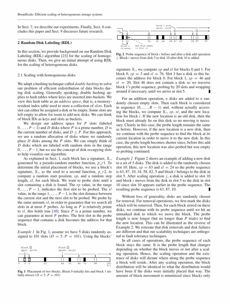
Example 1 In Fig. 1, assume we have 5 disks randomly as-signed to 101 slots (D = 5, P = 101). Using the blocks’

0 100193

Blocksp=3, sl=76

Blocksp=46, sl=20

46 66 865P-1

0 1

10

53 71

Fig. 1 Placement of two blocks. Block 0 initially hits and block 1 ini-tially misses (D = 5, P = 101)

63 8710 34 58 825

Block i withsp=63, sl=24

New disk addedto Slot 10

Block iis moved

41 48 69 97

Fig. 2 Probe sequence of block i before and after a disk add operationj . Block i moves from disk 5 to disk 10 after disk 10 is added

signature Xi , we compute sp and sl for blocks 0 and 1. Forblock 0, sp = 3 and sl = 76. Slot 3 has a disk so this be-comes the address for block 0. For block 1, sp = 46 andsl = 20. Slot 46 does not contain a disk so we traverseblock 1’s probe sequence, probing by 20 slots and wrappingaround if necessary, until we arrive at slot 5.

For an addition operation, n disks are added to n ran-domly chosen empty slots. Then each block is consideredin sequence (0, . . . , B − 1) and, without actually access-ing the blocks, we compute Xi , sp, sl, and the new loca-tion for block i . If the new location is an old disk, then theblock must already lie on this disk so no moving is neces-sary. Clearly in this case, the probe length remains the sameas before. However, if the new location is a new disk, thenwe continue with the probe sequence to find the block at itscurrent location in order to move it to the new disk. In thiscase, the probe length becomes shorter since, before this addoperation, this new location was also probed but was emptyso probing continued.

Example 2 Figure 2 shows an example of adding a new diskto a set of 5 disks. The disk is added to the randomly chosenslot 10. Here, sp = 63 and sl = 24 so the probe sequenceis 63, 87, 10, 34, 58, 82, 5 and block i belongs to the disk inslot 5. After scaling operation j , a disk is added to slot 10and block i moves from the disk in slot 5 to the disk in slot10 since slot 10 appears earlier in the probe sequence. Theresulting probe sequence is 63, 87, 10.

Without loss of generality, disks are randomly chosenfor removal. For removal operations, we first mark the diskswhich will be removed. Then, for each block stored on thesedisks, we continue with its probe sequence until we hit anunmarked disk to which we move the block. The probelength is now longer (but no longer than P trials) to findthe new location. This can be illustrated as the reverse ofExample 2. We reiterate that disk removals and disk failuresare different and that our scalability techniques are orthogo-nal to fault tolerance techniques.

In all cases of operations, the probe sequence of eachblock stays the same. It is the probe length that changesdepending on whether the block moves or not after a scal-ing operation. Hence, the scaling operation and the exis-tence of disks will dictate where along the probe sequencea block will reside. After any scaling operation, the blockdistribution will be identical to what the distribution wouldhave been if the disks were initially placed that way. Theamount of block movement is minimized since blocks only

S.-Y. D. Yao et al.

move from old disks to new disks. For any sequence of scal-ing operations, RDL will result in a uniform distribution ofblocks across homogeneous disks since blocks have an equalchance of falling into any slot. Also, blocks are quickly ac-cessible since locating blocks only requires a maximum ofP probes within the memory-resident address space.

Finally, there is a trade-off between large and small Pvalues [23]. We want to set P to a large enough value toallow for more scale-up room since the maximum numberof disks that the storage system can scale up to is P . How-ever, large P’s require more probing since there are moreempty slots to probe. Ideally, the growth rate of the storagesystem should be gauged beforehand to determine a goodP . A system administrator could estimate the growth rate ofthe system and chose a P value which is effective for a cer-tain amount of time. Once the number of disks reaches P(i.e., the slots are exhausted), a complete reorganization ofthe data blocks is required in order for P to be increased toallow for further scale-up.

2.2 Scaling with heterogeneous disks

In a heterogeneous disk system with different capacities andbandwidths, certain disks will tend to be favored more thanothers. If a disk has, for example, twice the bandwidth andcapacity of the others, we want twice the amount of blockshitting it. This means that the block assignments will not beuniform and must follow some weighting function, whereeach disk has an associated weight. We can achieve this byapplying the filter method to RDL so that blocks do not endup on the first disk they hit in their probe sequence. Instead,they probe disks one-by-one until the filter method finds atarget disk, based on the disk weight. The higher the weight,the more likely its corresponding disk will be a hit. We de-scribe this method below as well as discuss its main draw-back of extra block moves.

Given any block i , let the following denote its probe se-quence: P = {d0, d1, . . . , dD−1} where d j is a disk and is

0

f = 1/20

1

f = 11

Probe sequence

f = 1/30

0

f = 1/21

Probe sequence

1

f = 12

0

f = 1/30 f = 1/21

Probe sequence

1

f = 12

2

When adding a disk to a position other than the front of the probe sequence block movement from an old disk to another old disk will occur.

Block that fall in this range will be evenly distributedbetween disks 2 and 1.

0

1

0

1

0

1

0

1

0

1

0

1

0

1

0

1

a. b.

c.

2

Fig. 3 Figure 3a shows an initial group of two disks. Disk 2 is added to the front of the probe sequence in Fig. 3b and to the middle in Fig. 3c

unique within the probe sequence. Moreover, disk weightsare assigned based on their bandwidth and capacity. We givedetails on determining disk weights in Sect. 3. The corre-sponding weights for the disks that are probed are given by:W = {w0, w1, . . . , wD−1}.

We now use the filter method for placing block i on adisk along its probe sequence. We define a filter value foreach of block i’s probes: F = { f0, f1, . . . , fD−1} where:

f j = w j∑D−1

k= j wk(1)

It is easy to see that 0 < f j ≤ 1 for all j and fD−1 = 1.In order to determine which disk this particular block be-longs to, we use its signature Xi and the disk identifier, d j ,as seeds to a multi-seeded pseudo-random number functionto generate a pseudo-random number r j between 0 and 1.Starting with j = 0 to D − 1, we find the first disk d j of P ,where r j ≤ f j , to put block i .

We can now easily apply the filter method directly toRDL with varying disk weights by using filter values com-puted from Eq. 1. However, block movement after scalingwill not be minimized in this way. The movement can onlybe minimized (moving only from old to new disks) if disksare added to or removed from the front of the probe se-quence. Since every block has a different probe sequence,this will not be possible so some blocks will move from olddisks to other old disks.

Thus, this characteristic of the filter method is undesir-able and violates Requirement 2 (minimal data movement).Example 3 illustrates the additional amount of block move-ment when disks are not added to the front of the probe se-quence using the filter method with RDL.

Example 3 Consider a homogeneous case of the filtermethod with RDL where initially D = 2. In Fig. 3a,P = {0, 1}, W = {1, 1}, and F = {0.5, 1}. Using Xi andd0 = 0 as seeds, we compute a pseudo-random number, r0.If r0 ≤ 0.5 we place block i on disk 0, or disk 1 otherwise.

BroadScale: Efficient scaling of heterogeneous storage systems

In Fig. 3b, we add disk 2 to the front of the probe sequence.Here, P = {2, 0, 1}, W = {1, 1, 1}, and F = {0.33, 0.5, 1}.We recompute r0 using Xi and d0 = 2 as seeds. If r0 ≤ 0.33we place it on disk 2, otherwise we compute r1 using Xi andd1 = 0 as seeds. Now if r1 ≤ 0.5 block i is placed on disk0, or disk 1 otherwise. In this case, if block i moves, it onlymoves from an old disk to a new disk. However, in Fig. 3c,if disk 2 is added between disk 0 and 1, then block i couldmove from disk 0 to disk 1, old disk to old disk.

Even though the filter method does not work directlywith RDL for heterogeneous disks, we will use a similarfilter method as a component of our BroadScale algorithmdescribed later in Sects. 4 and 5. In Sect. 3, we introduceBroadScale, an algorithm similar to RDL, which maps mul-tiple slots to a single disk to support heterogeneous disks.

3 Disk weights

We have shown how RDL [23] can scale the size of a multi-disk system consisting of homogeneous disks using a ran-dom placement of the data. With the introduction of hetero-geneous disks, a uniform distribution of blocks from RDLwill not enable the disks to be fully utilized, assuming that allblocks are equally popular. In general, larger and faster disksshould hold more blocks. Using the filter method with RDLattempts to achieve this, as described in Sect. 2.2, but leadsto an undesirable characteristic of additional block moves.

In this section, we will describe our technique calledBroadScale which extends RDL for the support of hetero-geneous disks. BroadScale is based on RDL but the maindifference is that each disk can be mapped to multiple slotsdepending on the weight value of the disk. In Sect. 3.1, wedescribe how to compute disk weights assuming a staticgroup of disks that have different bandwidth to space ra-tios (BSR). In Sect. 3.2, we describe how to compute diskweights for a dynamically growing group of disks.

3.1 Disk weights for a static disk group

Instead of using the filter method directly with RDL, Broad-Scale assigns multiple slots to a single disk. The more slotsassigned to a disk, the more blocks this disk will contain.We call the number of slots assigned to a particular disk theweight of the disk. Each disk may or may not have a differentweight depending on its two characteristics: bandwidth5 andcapacity, measured in bits/second and bytes, respectively.Computing the weight from a combination of bandwidth andcapacity is also described in [8]. Clearly, a disk of weight 10will have twice as many blocks assigned to it than a disk ofweight 5.

The weight of disk d is unitless and is computed byits normalized bandwidth Bd/BMAX or normalized capacity

5 For simplicity, we use the average bandwidth since multi-zoneddisks have various bandwidth characteristics.

Cd/CMAX or a combination of both. When both bandwidthand capacity are considered, a system administrator couldoptionally set the weight to w′

d according to:

w′d = Bd

BMAX× β + Cd

CMAX× (1 − β) (2)

where β is the percentage of bandwidth contribution to w′d .

β is a tuning mechanism for the system administrator to ad-just between the priorities of bandwidth and capacity. BMAXand CMAX can be set to estimated future maximum band-width and capacity values. Since w′

d ’s could be fractionalnumbers, we can divide them by wG , which is the greatestcommon factor (GCF)6 of the w′

d ’s, to obtain integer valuesfor the weights. Hence, the disk weight, wd , is computedusing:

wd = w′d

wG(3)

Note that this assumption of wd being an integervalue may change when new disks are added resulting inweight fragmentation. Later, we reduce this fragmentationin Sects. 4 and 5.

Example 4 Suppose we have 2 disks where B0 = 10 MB/s,C0 = 20 GB, B1 = 20 MB/s, and C1 = 40 GB. If thedisk weights should only depend on bandwidth (β = 1) andBMAX = 40 then wG = 0.25, w0 = 1, and w1 = 2.

When computing disk weights, inefficiencies arise whenthe bandwidth to space ratio (BSR) of the disks are not allidentical. If β = 1 then the number of blocks on disks de-pends solely on their bandwidth where wd = Bd/wG . Thestorage capacity utilized on each disk will be equivalent tothe capacity of the disk with the highest BSR. Thus, somecapacity will be left unused on those disks with lower BSRs.However, a restriction may occur on disks with higher BSRs.These disks will fill up more quickly than other disks sincethey have proportionally less capacity. In this case, the band-width of these disks will not be fully utilized. To create moreroom on these disks, more disks need to be added.

In Fig. 4a, wd = 1 for d = 0, 1, 2 so each disk is as-signed to one slot and receives an equal number of blocks.Disks 0 and 1 have under-utilized storage capacities becauseβ = 1, indicating that the aggregate bandwidth should befully-utilized. Hence, the maximum aggregate amount ofuseful storage is the capacity of the disk with the highestBSR multiplied by D.

On the other hand, if β = 0 then the amount of blockson disks depends solely on their capacity so larger diskswill contain more blocks, even if they have little bandwidth.Here, wd = Cd/wG . The bandwidth of disks with lowerBSRs will be more stressed since they have proportionallyless bandwidth than disks with higher BSRs. In this case,disks are restricted by their bandwidths since they might

6 Since GCFs are traditionally integers, we can multiply the w′d val-

ues by 10x (where x is a user-defined precision value), truncate themto a whole number, and find the GCFs for these values instead.

S.-Y. D. Yao et al.

BSR = 0.31

BSR = 0.61

BSR = 1.23

Slots

C =148 GB

0

C =37 GB

2

C =74 GB

1

β = 1 BSR = 0.31

BSR = 0.61

BSR = 1.23

Slots

C =148 GB

0

C =37 GB

2

C =74 GB

1

β = 0w = 1d

w = 1d

w = 1d

w = 4d

w = 2d

w = 1d

a. b.

Disk 0 Disk 1 Disk 2 Disk 0 Disk 1 Disk 2

Fig. 4 Figure 4a shows unused capacity in disk 0 and 1 when β = 1. Figure 4b shows potential bottlenecks at disk 0 and 1 when β = 0.Bd = 45.5 MB/s for all disks

be slowed considerably. Figure 4b shows an example ofthis case where disks 0 and 1 contain more blocks thandisk 2 but all have the same bandwidth. Since all blockshave an equal chance of being accessed, more block re-quests will be delivered to disks 0 and 1, creating potentialbottlenecks.

Therefore, we can determine the weight of disk d usingEq. 3 to obtain an integer weight value that can map slots todisks. Next, we explore how to determine disk weights for adynamically growing disk group.

3.2 Disk weights for a dynamic disk group

Since we allocate slots (and therefore blocks) to disks ac-cording to the weight of each disk, dividing the weight by afactor will have the effect of changing the number of slotsallocated to the disk. Let’s use w′

F to denote the dividingfactor in general. The trade-off is that small w′

F values leadto larger wd values, which tend to make any fractional valueof the weight relatively insignificant but will require moreslots. Having more slots increases the storage requirementsof the address space, but more significantly, increases the to-tal amount of probing to locate blocks [23]. On the otherhand, larger w′

F values lead to smaller wd values whichcould result in under-utilized disk resources due to the moresignificant fractional value of the weight.

Trend reports, such as [7], of the growth rate of magneticdisk technology allow us to estimate the characteristics ofdisks that will be manufactured in the near-future. We canuse these estimations to help us determine w′

F . For example,if a system administrator anticipates adding new disks oneyear from now, w′

F can be computed from estimations ofthese disks’ characteristics given the current trend of tech-nology.

However, when disks are added to the system muchlater in the far-future, estimations of their characteristics(and therefore w′

F values) are more inaccurate. This in-accuracy could lead to fractional weight values and causeunder-utilization of new disks. Higher disk utilization canbe achieved by updating w′

F , however, this will impose highdata reorganization costs.

We can better utilize unpredictable far-future disks with-out using an over-abundance of slots by using an estimationof w′

F which we call the estimated common factor (ECF) ofthe total weight, or w′

E,α . The w′E,α of a new disk group is

computed such that the combined bandwidth and capacityusage will be at least α percent. w′

E,α is computed by Eq. 4:

∑D−1j=0 (w′

j mod w′E,α)

∑D−1j=0 w′

j

= 1 − α

100(4)

where D is the total number of disks in the new groupand the numerator adds up all the fractional portions of theweights.

Therefore, w′E,90 gives the ECF of the aggregate weights

such that the utilization is at least 90%. Figure 5 shows thelargest value of w′

E,90 that still achieves at least 90% uti-lization. Since far-future adds most likely involve disks withhigher bandwidth and larger capacity, the weights of thenew disks will be larger, thus the fractional weight portionwill be smaller. For the rest of this paper, we refer to frac-tional weight values as the weight fragmentation of a groupof disks. Fragmented weights, caused by the shaded regionsin Fig. 5, lead to an under-utilization, or waste, of the diskweight (e.g., a weight of 3.5 has .5 of wasted weight).

We arrive at Eq. 5 which maintains at least an α percentof utilization for near- and far-future scaling operations.

wd = w′d

w′E,α

(5)

ECF

ECF

ECF

ECF ECF

ECF

ECF

ECF

ECF

Total shadedregion is 10%of total diskbandwidth.

Total unshadedregion is 90%of total diskbandwidth.

ECF

Fig. 5 Total bandwidth of four disks. In this case, w′E,90 is the ECF

BroadScale: Efficient scaling of heterogeneous storage systems

Note that wd may not be an integer value when a hetero-geneous disk d is added. This is a problem since wd is thenumber of slots assigned to disk d , which of course cannotbe fractional. In Sects. 4 and 5, we describe two approachesfor reducing the waste associated with weight fragmenta-tion.

4 Disk clustering

The disk weights, as described in the previous section, mightbe fragmented and hence cannot be mapped directly to aninteger number of slots in RDL’s address space. In this sec-tion, we explore how to map fragmented disk weights toslots using disk clustering where clusters have almost inte-ger weights. For example, a disk weight of 1.5 cannot bemapped to 1.5 slots, but it can be clustered with another diskof weight 2.5 and mapped together to four slots. The idea isto try to reduce the fractional portion of the aggregated diskweights in each cluster as much as possible. Then each clus-ter is assigned to one or more slots instead of each disk beingassigned to slots. Actually, now the slots have no knowledgeof the disks at all. The higher the cluster weight, the moreslots it is assigned to and the more blocks that will be as-signed to the cluster. A question that remains is that after ablock is assigned to a cluster, which disk should it reside onwithin the cluster?

For the rest of this section, we first describe the simplecase of clusters with only one disk. Then we show that us-ing multiple disks per cluster can reduce the waste of diskresources. Finally, we describe how to locate a disk within adisk cluster for block assignment. We are not concerned withthe terms disk bandwidth and capacity in our discussions inSects. 4 and 5 since they have both been translated into theconcept of disk weights.

4.1 Single disk clusters

One method to accommodate disks with fragmented weightsis to simply use �wd� as the weight of disk d . Effectively,this method uses disk clusters that each contain only onedisk. For each cluster, the maximum amount of waste wouldthen be less than one unit of weight.

If the weights of new disks are relatively high then thepercentage of waste may not be significant. However, somelow disk weights may actually be less than 1 in which casethey cannot be mapped to any slots and are, in effect, unus-able. The single-disk cluster solution may suffice for steadyor increasing disk weights as disks are added, but is clearlyinadequate for fragmented, low disk weights.

4.2 Multiple disk clusters

By logically clustering multiple disks together, we can re-claim the fractional portions of the disk weights and re-duce the amount of waste. Instead of using individual disk

weights, cluster weights map a cluster of one or more disksto the appropriate number of randomly chosen slots.

The fragmentation of a cluster’s weight can decrease asdisks are added to the cluster. The cluster’s weight is the sumof its disks’ weights. The objective is for the cluster weight,wc, of cluster c to be as close to �wc� as possible. Since itmay be hard for wc to be exactly equal to �wc�, the clusteris said to be full when (wc − �wc�) ≤ (1 − ε). ε is specifiedby the user to indicate when a cluster is full (i.e., ε × 100percent full). Thus, when ε = 0.95, a cluster is full when thefractional portion of wc is less than 0.05. A new disk, d , iseither added to an existing non-full cluster or it is added toa new empty cluster by itself. The disk is added to a clustersuch that the fractional portion of wc is reduced after theinclusion of wd . In other words, disk d is added in such away that the overall waste of the storage system is reduced.

To decide where a new disk is added, we can generalizeour problem to the classical bin packing [4] problem. Theobjective of bin packing is to pack variable-sized items in asfew bins as possible thus, each bin becomes as full as possi-ble. Our main objective is also to pack each cluster as full aspossible with disks. For our problem, we will only considerthe fractional portion of the disk and cluster weights. Disksare items and clusters are bins, but the fractional portion ofthe disk weights are the item sizes and the clusters (bins) areof size 1. A slight difference to traditional bin packing is thata disk can only be packed into a cluster if it reduces the frac-tional portion of the sum of the disk sizes in that cluster. Aneasy way to translate this back to traditional bin packing isto use Eq. 6 to compute disk sizes:

s(wd) = 1 − (wd − �wd�) (6)

where wd is a disk weight and s(wd) is the disk size. Hence,by packing disks into clusters of size 1, the weight fragmen-tation of clusters is reduced.

With traditional bin packing, all items (disks) are knownbeforehand so an optimal packing arrangement does existeven though it cannot be found in polynomial time (an NP-hard problem). However, since we have no prior knowledgeof how many future disks there are, we must optimally rear-range the entire packing for each new disk, requiring mostblocks to be moved each time. Obviously, this solution is in-feasible. Therefore, we use a heuristic such as the Best Fit [4]algorithm to optimize the placement of just the next disk tobe added. Using Best Fit, disk d should be placed in a clusterthat has current size closest to, but not exceeding, 1−s(wd).If this results in multiple clusters then the one with the low-est index is chosen as the tiebreaker. If disk d does not “fit”into any of the clusters, a new cluster is created with disk d .Thus, Best Fit searches all the clusters and picks the best oneto which the disk should be added.

Large-scale storage systems may have on the order of10, 000 disks (e.g., Lustre) so an exhaustive search to findthe best cluster to place a disk may be computationally inten-sive. In these cases, the First Fit [4] algorithm may be moreappropriate since it simply picks the first cluster in which thedisk fits. First Fit and Best Fit are both good approximations

S.-Y. D. Yao et al.

0 1 43 2 657

Slots

320 1

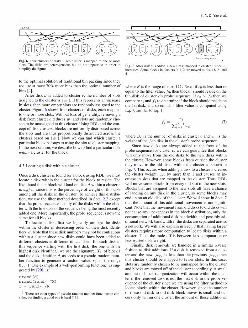
Fig. 6 Four clusters of disks. Each cluster is mapped to one or moreslots. The disks are heterogeneous but do not appear so in order tosimplify the figure

to the optimal solution of traditional bin packing since theyrequire at most 70% more bins than the optimal number ofbins [4].

After disk d is added to cluster c, the number of slotsassigned to the cluster is �wc�. If this represents an increasein slots, then more empty slots are randomly assigned to thecluster. Figure 6 shows four clusters of disks, each mappedto one or more slots. Without loss of generality, removing adisk from cluster c reduces wc and slots are randomly cho-sen to be unassigned to this cluster. Using RDL and the con-cept of disk clusters, blocks are uniformly distributed acrossthe slots and are thus proportionally distributed across theclusters based on �wc�. Now we can find which cluster aparticular block belongs to using the slot to cluster mapping.In the next section, we describe how to find a particular diskwithin a cluster for the block.

4.3 Locating a disk within a cluster

Once a disk cluster is found for a block using RDL, we mustlocate a disk within the cluster for the block to reside. Thelikelihood that a block will land on disk d within a cluster cis wd/wc since this is the percentage of weight of this diskamong all the disks in the cluster. To achieve this distribu-tion, we use the filter method described in Sect. 2.2 exceptthat the probe sequence is only of the disks within the clus-ter with the first disk of the sequence being the most recentlyadded one. More importantly, the probe sequence is now thesame for all blocks.

To locate a disk, first we logically arrange the diskswithin the cluster in decreasing order of their disk identi-fiers, d . Note that these disk numbers may not be contiguouswithin a cluster since new disks could have been added todifferent clusters at different times. Then, for each disk inthis sequence starting with the first disk (the one with thehighest disk identifier), we use the signature, Xi , of block iand the disk identifier, d , as seeds to a pseudo-random num-ber function to generate a random value, r0, in the range0 . . . 1. One example of a well-performing function,7 as sug-gested by [20], is:

srand(d)srand(rand()^X)r = rand()/R

7 There are other types of pseudo-random number functions to con-sider, but finding a good one is hard [13].

0 1 43 2 657

Slots

8

Probe sequence

320 1

Fig. 7 After disk 8 is added, a new slot is mapped to cluster 3 since w3increases. Some blocks in clusters 0, 1, 2 are moved to disks 8, 6, and4

where R is the range of rand(). Next, if r0 is less than orequal to the filter value, f0, then block i should reside on the0th disk of cluster c’s probe sequence. If r0 > f0 then wecompare r1 and f1 to determine if the block should reside onthe 1st disk, and so on. This filter value is computed usingEq. 7, similar to Eq. 1.

f j = w j∑Dc−1

k= j wk

(7)

where Dc is the number of disks in cluster c and w j is theweight of the j-th disk in the cluster’s probe sequence.

Since new disks are always added to the front of theprobe sequence for cluster c, we can guarantee that blockswill only move from the old disks to the new disks withinthe cluster. However, some blocks from outside the clustermay move to the old disks within the cluster as shown inFig. 7. This occurs when adding a disk to a cluster increasesthe cluster weight, wc, by more than 1 and causes an in-crease in slots that are mapped to the cluster. Thus, RDLwill move some blocks from every old slot to the new slots.Blocks that are assigned to the new slots all have a chanceof landing on any disk in the cluster, so some blocks mayend up on an old disk of the cluster. We will show in Sect. 7that the amount of this additional movement is not signifi-cant. Note that the movement from old disks to old disks willnot cause any unevenness in the block distribution, only theconsumption of additional disk bandwidth and possibly ad-ditional network bandwidth if the disks are separated acrossa network. We will also explain in Sect. 7 that having largerclusters requires more computation to locate disks within acluster. Thus, the trade-off is between less computation orless wasted disk weight.

Finally, disk removals are handled in a similar reversefashion as disk additions. If a disk is removed from a clus-ter and the new �wc� is less than the previous �wc�, thenthis cluster should be mapped to fewer slots. In this case,slots are randomly chosen to be unmapped from the clusterand blocks are moved off of the cluster accordingly. A smallamount of block reorganization will occur within the clus-ter if the removed disk is not the first disk in the probe se-quence of the cluster since we are using the filter method tolocate blocks within the cluster. However, since the numberof these old disk to old disk block moves is small and oc-curs only within one cluster, the amount of these additional

BroadScale: Efficient scaling of heterogeneous storage systems

moves is insignificant compared to the overall number ofmoves.

5 Fragment clustering

As described in the previous section, disk clustering is a wayto reduce the overall weight fragmentation by selectivelyadding disks to clusters, thereby reducing cluster weightfragmentation. Another approach to reducing weight frag-mentation is fragment clustering where only the fractionalportions of the disk weights are clustered together. Withfragment clustering, physical disks are mapped to 1 or morerandomly chosen slots. Then the fractional disk weight por-tions are grouped together into unit-sized logical disks andeach logical disk is mapped to 1 randomly chosen slot. Thedetails of this approach are described as follows.

When a new heterogeneous disk d is added to the storagesystem, it is mapped to �wd� randomly chosen slots in thevirtual address space. If the fractional portion of wd , namelywd − �wd�, is greater than 0, its fractional value, along witha pointer to disk d , is appended as an entry in the unit-sizedPending Logical Disk (PLD). Figure 8 shows an exampleof mapping a disk of weight 3.5 to 3 slots with the frac-tional weight .5 appended as an entry in the PLD. The frag-ment clustering algorithm maintains only one PLD, whichstores the currently unutilized weight fragments. The PLDbecomes full when the sum of its fractional values is greaterthan or equal to 1.0. Once this sum is greater than 1.0, thePLD becomes an Active Logical Disk (ALD), and the excessvalue of the sum (i.e., sum − 1.0), along with a pointer to d ,is stored as an entry in a newly allocated PLD. This ALD isnow mapped to a randomly chosen slot. Of course, the num-ber of ALDs increases as more disks are added, whereas weonly maintain one PLD.

Once the disks are mapped to slots in the manner justdescribed, data blocks can be assigned to disks using RDLas normal by probing the slots. Figure 9 illustrates the place-ment of block 1 directly onto a physical disk and block 2onto a physical disk via a logical disk (i.e., an ALD). Whena slot mapped to a physical disk is probed, that block isassigned to the disk. However, when a slot mapped to anALD is probed, further computation must be done to deter-mine which physical disk this block eventually resides on.To accomplish this, we use the filter method from Sects. 2.2

3.0

Slots

3.5

.5

PLD

Fig. 8 A disk of weight 3.5 is mapped to three slots. The .5 fractionalvalue along with a pointer to the disk is stored as an entry in the PLD.The PLD is activated into an ALD when it is full

3.0 2.0 3.0 .5 .5 .4 .6 .2ALD ALD

PLD

3.5 2.9 3.8

1 2

Physical Disks

not yetactive

Fig. 9 Block 1 probes slots using RDL until it lands on the disk withweight 3.5. Block 2 probes slots and lands on an ALD. Within theALD, the filter method determines Block 2 to hit the entry with value.6 and is forwarded to the disk with weight 3.8. Note that the pointerof the entry in the PLD is not yet active since the PLD is not yet full

and 4.3 on the ALD, which contains entries of fractional val-ues summing up to 1.0. Once an entry is found using the fil-ter method, the pointer within that entry is followed to thephysical disk where the block should be placed.

Since adding new disks will never cause updates to en-tries in the ALDs (but do cause PLD updates), we do notneed a specific initial ordering (i.e., least recently added tomost recently added) of the entries. However, once an ini-tial entry ordering is decided from the construction of thePLD, this ordering must remain the same after conversion toALDs.

With disk removals, there will be a small amount of ad-ditional block moves incurred due to the removal of entrieswithin ALDs. When a disk is removed, the entry containingthe fractional portion of its weight is also removed causingan ALD to have a weight of less than one. The remainingentries in the ALD can be combined with any entries in thePLD to become a full ALD and/or a partially filled PLD.Additional block moves will result when some blocks aremoved from non-removed disks to other disks. This will oc-cur during disk removals since removing an entry in an ALDwill unmap it from a slot and cause blocks in the remain-ing entries to be relocated. However, these additional blockmoves are also a small percentage of the overall moves.

Intuitively, using fragment clustering, the overall amountof weight fragmentation at any given time will always be lessthan 1.0. This fragmentation will only be contributed by thefractional values in the PLD. When the PLD fills to capacity(i.e., 1.0), it becomes active and its weight fragments areutilized. We show that this is true in Sect. 7.

In sum, BroadScale is a technique which first involvescomputing a weight for each disk based on bandwidth and/orcapacity as described in Sect. 3. If these weights are not in-teger values, then we have weight fragmentation and wasteddisk resources will arise. BroadScale reduces weight frag-mentation through two approaches, disk clustering and frag-ment clustering. Disk clustering strategically clusters diskstogether using either the Best Fit algorithm or the First Fitalgorithm to reduce fragmentation. Fragment clustering isanother approach where the fractional portion of the weights

S.-Y. D. Yao et al.

are grouped as logical disks. A comparison of disk cluster-ing with fragment clustering is discussed in Sect. 7 alongwith benefits and drawbacks of each.

6 Related work

We describe related work on two categories of applicationsto which we can apply our BroadScale algorithm. These cat-egories are redistributing CM blocks on CM server disks andremapping Web objects on Web proxy servers.

Previous literature on CM servers have discussed ar-eas such as distributed architectures and retrieval schedul-ing [11, 17]. The topic of homogeneous and heterogeneousdisk scaling in CM servers has been the focus of a few paststudies. One study mixes popular (hot) and unpopular (cold)CM data objects together on heterogeneous disks with dif-ferent BSRs [3]. Their objective is to maximize the utiliza-tion of both bandwidth and capacity while maintaining theload balance. However, the popularity of the objects need tobe known ahead of time to be properly placed. Moreover,their popularity might change over time (e.g., new moviestend to be accessed more frequently) so the objects mayneed to be moved depending on their current popularity.Other techniques stripe fixed-size object blocks, describedbelow, as opposed to storing them in their entirety.

Disk scaling with round-robin data striping is discussedin [5]. With round-robin, almost all blocks need to be relo-cated when scaling. The overhead of such block movementmay be amortized over a period of time but it is, never-theless, significant and wasteful. Wang and Du [22] de-scribe a technique which assigns weights to disks basedon bandwidth and capacity. However, they also distributedata blocks in a round-robin fashion, requiring large blockmovement overhead when scaling. Another technique calledDisk Merging [24] merges a static group of heterogeneousphysical disks into homogeneous logical disks to maximizebandwidth and capacity for striped data. This technique isnot intended for dynamic scaling since the system must betaken off-line and reconfigured, potentially reshuffling manyblocks.

While traditional constrained placement techniques suchas round-robin placement allow for deterministic serviceguarantees, random placement techniques are modeled sta-tistically. The RIO project demonstrated the advantages ofrandom data placement such as single access patterns andasynchronous access cycles to reduce disk idleness [12].However, they did not consider the dynamic rearrangementof data due to disk scaling. Although they do not requireprior knowledge of object popularity for full utilization ofheterogeneous disks’ aggregate bandwidth, their solution re-quires data replication for short- and long-term load balanc-ing [15]. In one scenario, they require at least 34% blockreplication for 100% bandwidth utilization. Another studyfocused on the trade-off between striping and replicationfor load balancing [2]. For large systems, the extra stor-age needed for replication becomes more significant. In gen-

eral, random placement, or pseudo-random in our case, in-creases the flexibility to support various applications whilemaintaining a competitive performance [16]. We developeda prior technique called SCADDAR that redistributes datablocks after homogeneous disk scaling in a CM server bymapping the block signatures to a new set of signatures foran even, randomized distribution [6]. SCADDAR supportsdisk additions just as well as disk removals. SCADDAR ad-heres to the requirements of Sect. 1 except that the com-putation of block locations become incrementally more ex-pensive. Finding a block’s location requires the computationof that block’s location for every past scaling operation, so ahistory log of operations must be maintained. In comparison,our RDL and BroadScale algorithms are fast in computationeven though they are limited by the total number of disks(i.e., P).

Another technique to scale heterogeneous disks is de-scribed in [8]. This technique attempts to achieve similarrequirements in load balancing, minimal block moves, andfast data access. However, its major drawback is that is doesnot allow disk removal scaling operations. Our SCADDAR,RDL, and BroadScale algorithms support both additions andremovals of homogeneous and heterogeneous storage de-vices.

Several past works have considered mapping Web ob-jects to proxy servers using requirements similar to thosedescribed in Sect. 1. Below we describe two relevant tech-niques called highest random weight (HRW) and consistenthashing along with their drawbacks.

HRW was developed to map Web objects to a group ofproxy servers [20]. Using the object name and the servernames, each server is assigned a random weight. The ob-ject is then mapped to the highest weighted server. Afteradding or removing servers, objects must be moved if theyare no longer on the highest weighted server. The drawbackhere is that the redistribution of objects after server scalingrequires B × D random weight function calls where B isthe total number of objects and D is the total number ofproxy servers. A simple heterogeneous extension to HRW isdescribed in [14], but suffers from the same computationalcomplexity. We show in [23] that in some cases HRW is sev-eral orders of magnitude slower than our RDL technique. Anoptimization technique for HRW involves storing the ran-dom weights in a directory, but the directory size will in-crease as B and D increase causing the algorithm to becomeimpractical.

Consistent hashing is another technique used to mapWeb objects to proxy servers [9]. Here objects are onlymoved from two old servers to the newly added server. Avariant of consistent hashing used in a peer-to-peer lookupserver, Chord, only moves objects from one old server to thenew server [19]. In both cases, the result is that objects maynot be uniformly distributed across the servers after serverscaling since objects are not moved from all old servers tothe new server. With Chord, a uniform distribution can beachieved by using virtual servers, but this requires a consid-erable amount of routing meta-data [1].

BroadScale: Efficient scaling of heterogeneous storage systems

7 Experiments

In this section, we describe our simulation experiments tovalidate our BroadScale algorithm. First, we show that datablocks are distributed across the disks according to the diskweights. The higher the weight, the more blocks will resideon the corresponding disk. Next, we measured the amountof weight fragmentation from disk clustering and fragmentclustering. With disk clustering, varying the size of the clus-ters affects the amount of fragmentation. Then, we show thatthe additional amount of block movement using disk clus-tering is not significant compared to the overall number ofmoves. This movement is even lower with fragment cluster-ing. Finally, the average and maximum number of probes isshown for disk and fragment clustering.

For all of our experiments, we distributed approximately750, 000 blocks across 10 initial disks, which is a realisticstarting point. We set the total number of slots to 1, 511(i.e., P = 1, 511) because we need room to add disks andmultiple slots are mapped to each disk depending on the diskweight. We computed disk weights for a dynamic disk groupusing Eq. 5 by setting β = 1, where the number of blocks ondisks depends solely on disk bandwidth. We set α = 90%so that at least 90% of the aggregated disk weight is uti-lized to determined the number of blocks per disk. Whensimulating disk scaling, we assume a 10-disk add operationis performed every 6 months. For this time period, industrytrends suggest that disk bandwidth increases 1.122× in [7],and disk capacity increases 1.26× following Moore’s Law.Our added disks follow these trends.

The disk weights are used to indicate how many blocksshould reside on a disk relative to other disks. Since thenumber of slots assigned to a disk is roughly equal to thedisk weight, more slots assigned to the disk will result inmore blocks for the disk. Figure 10 shows blocks distributedacross 10 disks by BroadScale. For illustration purposes,these disks vary widely in bandwidth and, therefore, inweight. After distributing the blocks, the trend of the amountof blocks per disk follows the trend of the disk weights. The

0

20000

40000

60000

80000

100000

0 1 2 3 4 5 6 7 8 9Disk number

# o

f b

lock

s p

er d

isk

0

1

2

3

4

5

6

7

8

9

Disk w

eigh

t

# blocks per disk # blocks/weight Disk weight

Fig. 10 The number of blocks per disk follows the same trend as thedisk weight

blocks per disk (w.r.t. the left axis) and the disk weights(w.r.t. the right axis) are overlaid together on the same fig-ure to show their similarity. Moreover, as expected, Fig. 10shows that the normalized curve (w.r.t. the left axis) is quiteuniform across disks. The normalized curve is computed as(blocks on disk d/weight of disk d).

We assume that all data blocks have a similar probabil-ity of being accessed. However, the block access will be loadbalanced even for skewed access distributions, such as a Zipfdistribution, when storing a large number of files using ran-dom block placement. If certain files are more popular thanothers, the blocks in these popular files will be randomly dis-tributed across all the disks just as the blocks in unpopularfiles. In this case, the number of popular blocks on each diskis similar. Furthermore, certain blocks within a file may bemore popular than other blocks within that file. Again, ran-domly distributing all blocks will result in a similar numberof popular blocks on each disk.

Disk clustering and fragment clustering were two tech-niques introduced in Sects. 4 and 5. The purpose of cluster-ing is to reduce the fragmentation of the disk weights, thusreducing the waste, so that each disk will hold a more ac-curate number of blocks. Figure 11 shows the aggregatedwaste of disk weights using both techniques as the storagesystem is scaled by adding 10 disks at a time with 10 ini-tial disks. For disk clustering, we want to show that the to-tal amount of unutilized disk weight decreases as clustersincrease in size. When the maximum cluster size, KMAX,is 1, the effect is that there is no clustering. Here, disk dis assigned to �wd� slots and the amount of wasted diskweight is significant. However, increasing KMAX to 2 givesus much better weight utilization since the clusters are com-bining fragmented weights. Furthermore, setting KMAX = 3leads to even greater improvement. We found that disk clus-ters became full at 3 disks, which is the expected valueof the cluster size, so increasing KMAX beyond 3 gave noimprovement.

0

10

20

30

40

50

60

10 20 30 40 50 60 70 80 90 100

Disk cluster size = 1Disk cluster size = 2Disk cluster size = 3

# of disks (after 10-disk add operations)

Aggregated weight fragmentation

Fragment clustering

Fig. 11 The overall amount of weight fragmentation using disk clus-tering and fragment clustering

S.-Y. D. Yao et al.

Using the Best Fit algorithm for disk clustering, the ex-pected value, E(Dc), of the number of disks on cluster c canbe determined by analyzing the fractional part of the diskweights. Given a disk weight, the expected value of the frac-tional portion is .5. The second weight must reduce the frac-tional portion when summed with the first, so the expectedvalue becomes .25. Each time a weight is added in this way,the expected fractional value is halved so we have:

0.5E(Dc) = 1 − p (8)

where p is the precision of E(Dc) since 0.5E(Dc) will neverequal 0. For example, with a precision of 0.94, E(Dc) = 4disks. Solving for E(Dc), we arrive at the following:

E(Dc) = log0.5(1 − p) (9)

Fragment clustering demonstrates the best performancesince the maximum amount of total fragmentation is alwaysless than a weight of 1.0. This is attributed to the fractionalvalues stored in the PLD. However, with fragment cluster-ing, newly added disks are almost never fully utilized sincethe PLD contains weight fragments only from these recentlyadded disks. Nevertheless, this may become insignificant asthe disk weights increase.

There exists a trade-off between low computation andlow weight fragmentation for disk clustering since findingwhich disk within a cluster a block resides requires less com-putation for smaller clusters. To find a block located in clus-ter c using the filter method, on average, the pseudo-randomfunction is invoked for half of the disks in c. Hence, finding adisk within small clusters requires less computation, but re-sults in more weight fragmentation. However, since the ex-pected number of disks per cluster, from Eq. 9, is low andwe observe low weight fragmentation in Fig. 11 with smallclusters (of size 3), high computation is not required. Forfragment clustering, we cannot change the size of the PLD,but the number of PLD entries is low so finding a particularentry using the filter method is not costly. Below, we observethe overall amount of block movement of disk and fragmentclustering.

In Sect. 4.3, we explained that adding disks could causemore blocks to be moved than the minimum that is re-quired to fill the new disks. This is true of both clusteringapproaches. With disk clustering, the additional moves de-pends on the cluster size. If a disk is added to a new emptycluster, no extra moves are incurred. If a disk is added toa non-empty cluster, some blocks will be moved to the olddisks in that cluster in addition to the new disks. Similarly,fragment clustering will result in these redundant moveswhen adding a disk causes the conversion of a PLD to anALD. Since the PLD contains fractional entries from olddisks, activating the PLD to an ALD will redistribute datafrom old disks to these old entries. However, the amount ofthese data moves is low since one ALD is a small componentof the entire storage system.

Figure 12 shows the total amount of block movementwhen scaling disks 10 at a time with 10 initial disks. Here

0

50000

100000

150000

200000

250000

300000

350000

400000

450000

500000

10 20 30 40 50 60 70 80 90 100

# of disks (after 10-disk add operations)

Tot

al #

of b

lock

mov

es

Old disk to new diskmovement

Old disk to old diskmovement

Fig. 12 The additional block movement (old disk to old disk) for diskclustering represents a small fraction of the total block movement

β = 1 so disk weights only represent the disk bandwidth,which grows 1.122× every scaling operation. We observethat the percentage of block moves from an old disk to an-other old disk is on average 13% of the total moves fordisk clustering. Since cluster sizes tend to be small, fromEq. 9, and using small clusters is effective, the additionalmovement will not be a significant percentage of the total.We notice a decreasing trend in total block moves since the10 disks that are added each time require fewer and fewerblocks to fill them, assuming the number of blocks is con-stant. A similar test on fragment clustering results in onlyaround 3% redundant moves since a new ALD is small com-pared to the actual added disks.

Figure 12 employs the industry growth rate of disk band-width. For other growth rates, the percentage of old disk toold disk block movement decreases as higher growth ratedisks are added for both clustering techniques. This is dueto the fractional weight portion being proportionally smallerthan the whole weight of these growing disks. Figure 13shows the percentage of this redundant block movement

0

2

4

6

8

10

12

14

16

5 10 15 20 25 30 35 40 45

Rate of bandwidth growth per scaling operation (%)

% o

f old

dis

k to

old

dis

k bl

ock

mov

emen

t

Disk Clustering

Fragment Clustering

Fig. 13 The average percentage of redundant block movement for var-ious growth rates

BroadScale: Efficient scaling of heterogeneous storage systems

0

20

40

60

80

100

120

140

160

10 20 30 40 50 60 70 80 90 100

# of disks

Ave

rage

pro

bes

5%

25%

45%

0

200

400

600

800

1000

1200

1400

1600

1800

10 20 30 40 50 60 70 80 90 100

# of disks

Max

imum

pro

bes

5%

25%

45%

Fig. 14 Average and maximum probes for bandwidth growth rates of 5, 25, and 45% (P = 10, 000)

with respect to the growth rate. For each growth rate value,the average percentage of redundant movement is measuredas disks are scaled. The average percentage is calculatedfrom 25 trials of each growth rate value with each trial usinga different randomness factor to slightly vary the disk char-acteristics. From Fig. 13, fragment clustering exhibits lessredundant movement than disk clustering. Redundant movesresults from blocks being redistributed into old disks of acluster and old fractional entries of an ALD in disk and frag-ment clustering, respectively. Fragment clustering has fewerredundant moves since it isolates these moves to just oneALD whereas disk clustering isolates these moves across anentire disk cluster.

Lastly, a higher growth rate when scaling disks shouldlead to less probing. The reason is that disks with largerweights will require more slots. This causes probing to bemore successful in general since there are fewer empty slotsand misses will be less frequent. Figure 14 shows the aver-age and maximum number of total probes as disks are scaled10 at a time beginning with 10 disks. The probing results ofdisk clustering and fragment clustering are similar and indis-tinguishable in the figure since the number of cluster group-ings in each technique are similar. Figure 14a shows that theaverage number of probes is lower when scaling disks at abandwidth growth rate of 45% than at a growth rate of 5%.Similar results are shown in Fig. 14b for the maximum num-ber of probes.

Fragment clustering appears to be superior to disk clus-tering in weight fragmentation and redundant block moves.However, one drawback of fragment clustering is the addi-tional bookkeeping required for the ALD entry pointers tophysical disks. Moreover, within the ALDs and the PLD, thefractional values must be stored with these pointers. Anotherdrawback is that newly added disks may not be fully utilizedsince their fractional weight portions are stored in the PLDand not yet activated.

8 Conclusions

BroadScale is a storage scaling algorithm that can benefitthe storage systems of digital libraries and archives. Broad-Scale allows additions or removals of heterogeneous disks

in a storage system where weights are assigned to disksdepending on their bandwidth and capacity characteristics.Blocks are distributed among the disks proportional to theseweights. Since only the integer portions of the weight valuescan be used to direct block placement, the fractional por-tions are wasted. However, these wasted portions, or weightfragments, can be strategically combined using either ourdisk clustering or fragment clustering approaches. Broad-Scale satisfies our scaling requirements of an even load ac-cording to disk weights, a minimum amount data movementwhen scaling disks, and the fast retrieval of data before andafter scaling.

We have shown through experimentation that blocks aredistributed proportionally to the disk weights using Broad-Scale. Disk scaling could lead to wasted disk weight (i.e.,weight fragmentation), but can be substantially reducedthrough clustering. We observed significant improvementusing larger cluster sizes in disk clustering. However, ourfragment clustering technique is superior in overall weightfragmentation as well as average percentage of redundantblock moves with a few minor drawbacks such as some ex-tra bookkeeping. Although fragment clustering outperformsdisk clustering, the additional block moves in either case wasnot significant compared to the total moves.

9 Future work

For future work, BroadScale can be extended to allow forscaling beyond P number of total disks by using an algo-rithm such as our previous algorithm SCADDAR [6]. Forheterogeneous scaling with SCADDAR, we could use a sim-ilar weight function and assign disk d to �wd� slots.

We believe BroadScale can be generalized to map anyset of objects to a group of scalable storage units. These ob-jects might also require a redistribution scheme to maintain abalanced load. Examples of other applications include Webproxy servers and extent-based file systems. Scalability inintegrated file systems that support heterogeneous applica-tions [18] may also benefit from BroadScale.

Furthermore, we wish to integrate fault tolerance mech-anisms with our scaling techniques. Each RDL slot is a stor-age unit which we assume to be a single disk drive. However,

S.-Y. D. Yao et al.

this storage unit can also represent a entire RAID device. Sowhen scaling, a RAID device can be either added to or re-moved from a slot. Another more integrated approach is tokeep primary block copies on the first disk of that block’sprobe sequence as usual and to add block replicas to the sec-ond disk of the probe sequence. We have shown that disksappear exactly once on every probe sequence so replicas areguaranteed to never be placed on the same disk as the pri-mary copies.

Finally, we wish to investigate how BroadScale could beapplied to storage systems that need to efficiently store ahigh influx of data streams such as those generated by large-scale sensor networks. We also want to explore data retrievalin large, scalable peer-to-peer systems or distributed hashtables. This requires a distributed implementation of Broad-Scale on top of these peer-to-peer search techniques.

Acknowledgements This research has been funded in part by NSFgrants EEC-9529152 (IMSC ERC), IIS-0082826 (ITR), IIS-0238560(PECASE), IIS-0324955 (ITR), IIS-0307908, CMS-0219463 (ITR),and a NASA/JPL grant and unrestricted cash gifts from Okawa Foun-dation and Microsoft. Any opinions, findings, and conclusions or rec-ommendations expressed in this material are those of the author(s)and do not necessarily reflect the views of the National ScienceFoundation.

References

1. Byers, J., Considine, J., Mitzenmacher, M.: Simple load balancingfor distributed hash tables. In: Proceedings of the 2nd InternationalWorkshop on Peer-to-Peer Systems (IPTPS ’03) (February 2003)

2. Chou, C.-F., Golubchik, L., Lui, J.C.S.: Striping doesn’t scale:how to achieve scalability for continuous media servers with repli-cation. In: Proceedings of the International Conference on Dis-tributed Computing Systems, pp. 64–71 (April 2000)

3. Dan, A., Sitaram, D.: An online video placement policy based onbandwidth to space ratio (BSR). In: Proceedings of the ACM SIG-MOD International Conference on Management of Data, pp. 376–385, San Jose, California (May 1995)

4. Garey, M.R., Johnson, D.S.: Computer and intractability: A guideto the theory of NP-completeness, Chapter 6, pp. 124–127. W. H.Freeman and Company, New York (1979)

5. Ghandeharizadeh, S., Kim, D.: On-line reorganization of data inscalable continuous media servers. In: 7th International Confer-ence and Workshop on Database and Expert Systems Applications(DEXA’96) (September 1996)

6. Goel, A., Shahabi, C., Yao, S.-Y.D., Zimmermann, R.: SCAD-DAR: An efficient randomized technique to reorganize continuousmedia blocks. In: Proceedings of the 18th International Confer-ence on Data Engineering, pp. 473–482 (February 2002)

7. Gray, J., Shenoy, P.: Rules of thumb in data engineering. In: Pro-ceedings of the 16th International Conference on Data Engineer-ing, pp. 3–10 (February 2000)

8. Honicky, R.J., Miller, E.L.: A fast algorithm for online placementand reorganization of replicated data. In: 17th International Par-allel and Distributed Processing Symposium (IPDPS 2003), Nice,France (April 2003)

9. Karger, D., Lehman, E., Leighton, T., Levine, M., Lewin, D.,Panigrahy, R.: Consistent hashing and random trees: Distributedcaching protocols for relieving hot spots on the World Wide Web.In: Proceedings of the 29th ACM Symposium on Theory of Com-puting (STOC), pp. 654–663 (May 1997)

10. Knuth, D.E.: The Art of Computer Programming, vol. 3. Addison-Wesley, Reading, MA (1998)

11. Martin, C, Narayan, P.S., B. Özden, Rastogi, R., Silberschatz,A.: The fellini multimedia storage server. In: Chung S.M. (eds.)Multimedia information storage and management, Chapter 5.Kluwer Academic Publishers, Boston (August 1996). ISBN: 0-7923-9764-9

12. Muntz, R., Santos, J., Berson, S.: RIO: A real-time multimedia ob-ject server. In: ACM Sigmetrics Performance Evaluation Review,vol. 25 (September 1997)

13. Park, S.K., Miller, K.W.: Random number generators: Good onesare hard to find. Commun. ACM, 31(10), 1192–1201 (1988)

14. Ross, K.W.: Hash-routing for collections of shared web caches.IEEE Netw. Mag., 11(6), 37–44 (1997)

15. Santos, J.R., Muntz, R.R.: Performance analysis of the RIO Mul-timedia Storage System with Heterogeneous Disk Configura-tions. In: ACM Multimedia, pp. 303–308, Bristol, UK (September1998)

16. Santos, J.R., Muntz, R.R., Ribeiro-Neto, B.: Comparing RandomData Allocation and Data Striping in Multimedia Servers. In: SIG-METRICS, Santa Clara, California (June 2000)

17. Shahabi, C., Zimmermann, R., Fu, K., Yao, S.-Y.D.: Yima: A Sec-ond Generation Continuous Media Server. IEEE Comput. pp. 56–64 (June 2002)

18. Shenoy, P., Goyal, P., Vin, H.M.: Architectural Considerations forNext Generation File Systems. Multimedia Syst., 8(4), 270–283(2002)

19. Stoica, I., Morris, R., Karger, D., Kaashoek, M.F., Balakrishnan,H.: Chord: A scalable peer-to-peer lookup service for internet ap-plications. In: Proceedings of the 2001 ACM SIGCOMM Confer-ence, pp. 149–160 (2001)

20. Thaler, D.G., Ravishankar, C.V.: Using name-based mappingsto increase hit rates. IEEE/ACM Trans. Network. 6(1), 1–14(1998)

21. Thomson, J., Adams, D., Cowley, P.J., Walker, K.: Meta-data’s role in a scientific archive. IEEE Comput. 36(12), 27–34(2003)

22. Wang, Y., Du, D.H.C.: Weighted striping in multimedia servers.In: Proceedings of the IEEE International Conference on Multi-media Computing and Systems (ICMCS ’97), pp. 102–109 (June1997)

23. Yao, S.-Y.D., Shahabi, C., Larson, P.-Å.: Hash-based labelingtechniques for storage scaling. The VLDB journal: The interna-tional journal on very large data bases (2004). ISSN: 1066-8888(Paper) 0949-877X (Online), DOI: 10.1007/s00778-004-0124-6,Issue: Online First.

24. Zimmermann, R.: Continuous media placement and scheduling inheterogeneous disk storage systems. Ph.D. Dissertation, Univer-sity of Southern California, Los Angeles, California (December1998)