implementation of koiter’s initial post-buckling theory
TRANSCRIPT

1
Commutativity of the Strain Energy Density Expression for the Benefit of the FEM
Implementation of Koiter’s Initial Post-buckling Theory
Shuguang Li1, Jiayi Yan1, Guofan Zhang2 and Shihui Duan2
1Faculty of Engineering, the University of Nottingham, Nottingham, NG7 2RD, UK
2AVIC Aircraft Strength Research Institute, Xi’an, 710065, PR China
Abstract
The concept of full commutativity of displacements in the expression for strain energy
density for the geometrically nonlinear problem has been introduced for the first time and fully
established in this paper. Its consequences for the FEM formulation have been demonstrated. As a
result, the strain energy, equilibrium equation and incremental equilibrium equation for the
geometrically nonlinear problem can all be presented in a unified manner involving various
stiffness matrices which are all symmetric, unique and explicitly expressed. As an important
application, the framework has been employed in the FEM implementation of Koiter’s initial post-
buckling theory, which has been handicapped by its mesh sensitivity in evaluating one of the initial
post-buckling coefficients. This has largely prevented it from being incorporated in mainstream
commercial FEM codes. Based on the outcomes of this paper, the mesh sensitivity problem has
been completely resolved without the need to use any specially formulated element. As a result,
Koiter’s theory can be practically and straightforwardly implemented in any FEM code. The results
have been verified against those found in the literature.
Keywords: Commutativity; Strain energy density; Geometrical nonlinearity; Finite element
formulation; Koiter’s theory; Initial post-buckling theory.
1 Introduction
The geometrically nonlinear problem has been perceived as well-established since analyses
of this kind are routinely carried out by users of commercial FEM codes, e.g. [1-3], as a standard
provision of these codes. However, there is one issue which has never been properly raised and
investigated, namely, the lack of commutativity of displacements in the various stages of FEM
formulation, all associated with the expression of strain energy density (SED) as will be explored in
the paper. The issue has always been sidestepped when encountered without being identified as a
problem but can be revealed straightforwardly if one attempts to derive the secant stiffness matrix.
Using conventional notations which are provided in Appendix A to avoid any confusion, the strain
energy in a finite element can be given as follows.
Accepted for publication in International Journal for Numerical Methods in Engineering, Jan 2018
2
1 1 1 1
2 2 2 4
1 1 1 1
2 2 2 4
e
e
e
L L L N N L N N
L L L N N L N N
U d
d
ε Cε ε Cε ε Cε ε Cε
q B CB B CB q B q CB B q CB q q
(1)
where e is the domain of the finite element concerned and q the nodal displacement vector
discretised from an otherwise continuous displacement field u. In order to establish the equilibrium
equation, variation of the strain energy (1) is required as given below, where advantage has been
taken of the symmetry of the C matrix, the obvious commutativity between q and q in
N B q q as explained in Appendix A and the fact that any term in the above expression, e.g.
1 1
2 2e
N Ld
q B q C B q , is a scalar and its transpose is equal to itself.
1 1
2 2e
e
L L L N N L N NU d
q B CB B CB q B q CB B q CB q q . (2)
The integral inside the square brackets in (2) should give the secant stiffness matrix of the element
but it has never been accepted because it lacks symmetry, as stated in the second edition of [4].
Whilst the first and fourth terms inside the integral are symmetric, the remaining part, i.e. the sum
of the second and third terms, does not look symmetric superficially because
T
1 1 1
2 2 2L N N L N L L N L N N L
B C B q B q CB B q CB B C B q B C B q B q CB . (3)
The above derivation followed the so-called N-notation (a terminology introduced in [9] as being
one approach to the FEM formulation, in contrast to the other commonly used approach referred to
in [9] as the B-notation) but has always been avoided in textbooks, e.g. [4-8], because it was seen as
a dead end. If one could swap the position of some of the displacements involved, e.g. the q and
the q at the end of the expression e
N Ld
q B q C B q , to give
e
N Ld
q B q C B q
without affecting the value of the expression, the inequality (3) would become an equality and the
secant stiffness matrix could readily be made symmetric. Unfortunately, commutativity in matrix
expressions is generally not applicable. Without a properly defined secant stiffness matrix,
equilibrium conditions cannot be stated in explicit form. Common practice is to establish
equilibrium indirectly by integrating stresses whilst jumping to the tangential stiffness matrix
directly [5-8] in terms of the formulation of element stiffness matrices, employing the so-called B-
notation [9]. There have been limited attempts [9-11] to unify expressions of secant and tangential
stiffness matrices but the obtained expressions lacked uniqueness, as admitted in [10,11]. It will be
shown later in this paper that the lack of symmetry and uniqueness is in fact a false impression. A

3
more fundamental and generic issue surfaces when one tries to implement Koiter’s initial post-
buckling theory [12] through FEM as it places more demands on commutativity of displacements in
energy expressions, referred to as full commutativity, as will be detailed later in this paper.
Existing accounts [13,14] of the FEM formulation of Koiter’s initial post-buckling theory
tended to shy away from having such commutativity fully established. There have not been many
attempts to adopt the N-notation for the FEM formulation in general since the publication of [13-
14], let alone its implementation for Koiter’s theory. The difficulty has been circumvented by
following the B-notation formulation of Koiter’s theory [15]. The price paid for this convenience is,
however, that the results become mesh sensitive as will be elaborated further in Section 6, noting
that mesh sensitivity is undesirable in any FEM analysis.
The objectives of this paper are twofold. On the fundamental theoretical development side,
it will establish the full commutativity of the SED as one of its intrinsic properties, and provide an
explicitly and uniquely presented FEM formulation in N-notation based on the full commutativity
established. The failure to appreciate such full commutativity is responsible for the fact that the
secant stiffness matrix has never been explicitly and uniquely obtained. This long-standing issue
will be resolved completely in this paper. On the practical side, and as a direct application of the
obtained fully commutative SED, the FEM implementation of Koiter’s theory using N-notation is
herewith made possible thus freeing it from the problem of mesh sensitivity that occurs in available
accounts. As will be introduced in more detail in Section 6 of this paper, Koiter’s theory provides
deep insight into the buckling problem of structures and hence has tremendous potential in practical
engineering applications. However, due to the lack of an acceptable FEM implementation, this
theory has been largely neglected, at least as far as mainstream commercial FEM codes are
concerned, wasting the opportunity to exploit it as a potentially valuable approach to address the
uncertainties associated with the buckling problem. The outcome of this paper will hopefully lead
to the resurrection of Koiter’s theory as a design analysis tool, providing structural designers and
engineers with the means to evaluate the confidence on their obtained buckling strengths of
structures. Lack of confidence in predicted results has been the main challenge to existing forms of
buckling analysis, the reason being the fact that some structures are extremely sensitive to initial
imperfections whilst others may be not. No assessment can currently be made of the sensitivity of
the obtained buckling load to the initial imperfection from the conventional buckling analysis and
Koiter’s theory fills this gap precisely and neatly, as will be further discussed in this paper.
2 The concept of full commutativity and apparent symmetry
The strain energy density U exists for any geometrically nonlinear problem and can be
expressed as a sum of homogeneous terms from the 1st to the 4th orders as follows
4
1 2 3 4U U U U U (4)
where the exact expressions of each term are provided in Appendix A.
Continuous displacement fields u, u , u and u are introduced to facilitate the following
discussion, and they are assumed to be mutually independent. They are discretised into q , q , q
and q for FEM applications, as already employed in expressing (1). In the context of Koiter’s
theory, these displacement fields can be the fundamental equilibrium path 0u , various orders of
perturbation displacements, 1u , 2u ,…, etc., respectively, as well as displacement variation u . In
order to illustrate the concept of commutativity, consider the strain energy at a specific deformation
state which is described as the sum of independent displacement fields. Take the third order term of
the SED as given in (A-5) in Appendix A for example
3
111 111 111 111 111 111
111 111 111 111 111 111
1
2
, , , , , , , , , , , ,
, , , , , , , , , , , ,
L NU
U U U U U U
U U U U U U
U
u u u u u u C u u u u u u
u u u u u u u u u u u u u u u u u u
u u u u u u u u u u u u u u u u u u
111 111 111 111 111 111, , , , , , , , , , , ,U U U U U u u u u u u u u u u u u u u u u u u
(5)
where 111
1, ,
2L NU u u u u C u u (6a)
111
1, ,
2L NU
u u u u C u u , … . (6b)
Relationship (5) introduces a trilinear form and its typical expression has been given in (6a). Some
of the displacements in (6a) can swap their positions without affecting the value of the expression,
e.g. u and u . In other words, 111 , ,U u u u is commutative as far as u and u are concerned.
This commutativity is described as partial commutativity of the trilinear form 111 , ,U u u u in the
present paper whilst u and u cannot be swapped without affecting the value of 111 , ,U u u u , in
general, because
111 111
1 1, , , ,
2 2L N L NU U
u u u u C u u u C u u u u u . (7)
In much the same way, a bilinear form 11 ,U u u and a quad-linear form 1111 , , ,U u u u u
can also be introduced from 2U and 4U , respectively,
11
1 1,
2 2N I L LU u u u u σ u C u (8)
1111
1, , ,
8N NU u u u u u u C u u . (9)
5
A property of full commutativity for bilinear, trilinear and quad-linear forms can be introduced as
one of the key subjects of the present paper if any pair of displacement fields involved in the
expression concerned can swap their positions in an expression without affecting the value of the
expression.
Along with full commutativity, another closely related property can be introduced as follows.
To formulate element stiffness matrices in FEM, it is desirable to express energy and its first and
second variations in a form of u Mu , with M being a matrix operator, as shown in (1) and (2), for
instance. However, not every term is readily given in this form explicitly, e.g. N I
u u σ as a
part of 11 ,U u u as given in (8). One of the tasks of the present paper is to make such terms into
u Mu form. Once a bilinear, trilinear or quad-linear form is so expressed, it will be referred to as
apparently symmetric in the present paper if M is given as a symmetric matrix operator. The lack
of symmetry in the secant stiffness matrix as shown in (2) resulted from the lack of such apparent
symmetry in the third order term of the SED.
Some of the difficulties in the FEM formulation of problems involving geometrical
nonlinearity resulting from the lack of full commutativity and apparent symmetry are listed as
follows.
1) Whilst the B-notation [9] delivers a symmetric tangential stiffness matrix [5-8], the secant
stiffness matrix cannot be obtained explicitly.
2) Following the N-notation [9], one can obtain the tangential and secant stiffness matrices
directly and make them symmetric [9-11]. However, without achieving the full
commutativity of SED, the obtained expressions of stiffness matrices lack uniqueness
[10,11].
Just as the secant and tangential stiffness matrices can be considered as the outcomes of the first and
second orders of variations of the strain energy, higher orders of variations are required in order to
implement the Koiter theory [12]. The earliest versions of FEM implementation of Koiter’s theory
tended to follow the N-notation [13,14] for the expressions of the so-called initial post-buckling
coefficients (IPBCs). However, the weaknesses of the N-notation as described above prevented it
from being practically exploited. Instead, alternative expressions for these IPBCs were brought
forward [15]. Unfortunately, they suffer from numerical ‘locking’ or mesh sensitivity [16,17]. The
solution to the problem has so far been either to employ a much more refined mesh than that used
for conventional buckling analysis in order to evaluate the IPBCs, or to employ specially
formulated elements [18-23], to name but a few of the available unattractive options.
It should be pointed out that, in analytical applications of Koiter’s theory, a displacement
field, such as the buckling mode or any perturbation modes at high orders, is described by a single

6
scalar giving the amplitude of an assumed pattern of the displacement field in the form of a scalar
function. Scalars are always commutative and commutativity has therefore never been an issue
there. In addition, the ‘locking’ problem is also absent in analytical approaches. However, the
applicability of analytical approaches is of course restricted to simple structures under simple
loading and boundary conditions, requiring FEM to be used for analysing structures of realistic
complexity, giving rise to the difficulty of mesh sensitivity. The present paper aims to demonstrate
that this difficulty can be removed by employing the N-notation after the establishment of the fully
commutative SED.
3 Fully commutative SED
Due to the symmetries of stress, strain and stiffness tensors and the definition of the Green
strain, the following relationships always hold.
N N u u u u (10a)
L L L L
u C u u C u (10b)
Given the above, it is clear that 11 ,U u u as given in (8) is already fully commutative, i.e.
11 11, ,U U u u u u . (11a)
However, relationships (10) deliver to 111 , ,U u u u and 1111 , , ,U u u u u only partial
commutativity between some pairs of u, u , u and u as follows.
111 111, , , ,U U u u u u u u (11b)
1111 1111 1111 1111
1111 1111 1111 1111
, , , , , , , , , , , ,
, , , , , , , , , , , , .
U U U U
U U U U
u u u u u u u u u u u u u u u u
u u u u u u u u u u u u u u u u (11c)
In general, however, commutativity cannot be blindly assumed between other pairs of u, u , u and
u , as may be observed from (7).
It is desirable to find alternative but equivalent expressions to 111U and 1111U , denoted as
111Q and 1111Q which are fully commutative, i.e.
111 111 111
111 111 111
, , , , , ,
, , , , , ,
Q Q Q
Q Q Q
u u u u u u u u u
u u u u u u u u u (12a)
1111 1111
1111
, , , , , ,
all together 24 permutations , , , .
Q Q
Q
u u u u u u u u
u u u u (12b)
As 11U is fully commutative, 11Q is identical to 11U .

7
The trilinear form is considered first. The expansion given in (5) offers a hint to the
construction of 111Q from 111U . If all possible permutations ( 3
3 3! 6P ) of u, u and u in 111U as
appearing in (5) have been included, one obtains
111 111 111
111
111 111 111
, , , , , ,, ,
, , , , , ,
U U UQ
U U U
u u u u u u u u uu u u
u u u u u u u u u. (13)
It is clear that swapping any pair of u, u and u only results in a reshuffle of the six terms inside
the brackets, e.g. between pair u and u
111 111 111
111 111
111 111 111
, , , , , ,, , , ,
, , , , , ,
U U UQ Q
U U U
u u u u u u u u uu u u u u u
u u u u u u u u u. (14)
Given the partial commutativity of 111U as shown in (11b), 111 , ,Q u u u given in (13) can be
reduced to
111 111 111 111, , 2 , , 2 , , 2 , ,
L N L N L N
Q U U U
u u u u u u u u u u u u
u C u u u C u u u C u u (15a)
The trilinear form 111 , ,Q u u u given above is thus fully commutative and it is straightforward to
verify that it satisfies (12a).
Similarly, a fully commutative fourth order expression 1111 , , ,Q u u u u can be
constructed from all 4
4 4! 24P possible permutations of u, u , u and u in 1111U . After
making use of the partial commutativity (11c), it can be expressed as
1111 1111 1111 1111, , 8 , , 8 , , , 8 , , ,
.N N N N N N
Q U U U
u u u u u u u u u u u u u u u u
u u C u u u u C u u u u C u u
, , (15b)
One can introduce functions 3Q u and 4Q u from 111Q and 1111Q as
3 111 3 111
1, , , ,
6Q Q U U u u u u u u u u (16a)
4 1111 4 1111
1, , , , , ,
24Q Q U U u u u u u u u u u u . (16b)
It is clear that 3Q and 4Q are identical to 3U and 4U in their roles as parts of the SED, respectively,
but 3Q and 4Q are associated with the fully commutative trilinear and quad-linear forms. If 3Q and
4Q are employed instead of 3U and 4U in the SED, they will not alter the value of SED in any way.
However, any subsequent manipulations on the displacement in the relevant energy term, such as
variations, will be indifferent to the position of the displacement within the expression, as a
straightforward and important application of the full commutativity, i.e.
8
3 111 111 111
111 111 111 12
1 1 1, , , , , ,
6 6 6
1 1 1 , , , , , , ,
2 2 2
Q Q Q Q
Q Q Q Q
u u u u u u u u u u
u u u u u u u u u u u
(17a)
and similarly
4 1111 13
1, , , ,
6Q Q Q u u u u u u (17b)
2
3 111 21, , 2 ,Q Q Q u u u u u and 2
4 1111 22
1, , , ,
2Q Q Q u u u u u u . (18)
where the subscripts correspond to the order of the variable in the variable list in the same way as
was originally introduced by Koiter in [12]. The SED expression obtained through 3Q and 4Q will
be called the fully commutative SED. With this property, the variations of them resemble the
derivatives of power functions. However, if 3Q and 4Q are directly derived from (16) with 3Q
and 4Q with 111Q and 1111Q as expressed in (15), one might still find the lack of apparent symmetry
at some points resembling the observation made to (2). It should be pointed out that the full
commutativity was taken for granted in [12] by Koiter without proof or guidance how to obtain this
property in general. Given the full commutativity as an intrinsic property of SED established
mathematically above, it is now known with assurance that the matrix involved in (2) is symmetric,
although this symmetry is not yet obvious. The lack of apparent symmetry in (2) is only due to the
way in which the expression is presented. Apparent symmetry will emerge after various terms
obtained above have been further streamlined by applying to them an identical transformation to be
described in the next section.
4 The flip transformation
The second order term in the Green strain gives rise to a factor of N u u appearing in
various places as shown above. Whilst the displacements involved in it are commutative, as shown
in (10a), many energy terms involving this do not have apparently symmetric appearances, i.e. not
in a form of u Mu with M being a symmetric matrix operator. For instance, u and u in
N I
u u σ as a term in U11 are both located biasedly on the same side of Iσ . They tend to cause
difficulties in FEM formulation if not treated appropriately. In fact, these terms can be expressed
differently in appearance but identically in value. One can easily prove the following relationship.
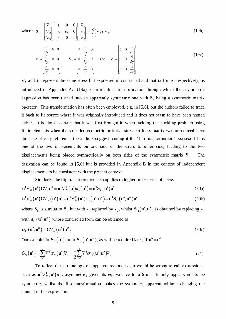
N I I I
u u σ u S u u S u (19a)
9
where 1 1 3
2 2
1
3 3
0 0
0 0
0 0
I
I I i I i
i
I
s
S s s
s
, (19b)
1 2 3
0 0 0 0 0 0
0 0 , 0 0 and 0 0 .
0 0 0 0 0 0
x x x
y y y
z z z
(19c)
Iσ and Is represent the same stress but expressed in contracted and matrix forms, respectively, as
introduced in Appendix A. (19a) is an identical transformation through which the asymmetric
expression has been turned into an apparently symmetric one with IS being a symmetric matrix
operator. This transformation has often been employed, e.g. in [5,6], but the authors failed to trace
it back to its source where it was originally introduced and it does not seem to have been named
either. It is almost certain that it was first brought in when tackling the buckling problem using
finite elements when the so-called geometric or initial stress stiffness matrix was introduced. For
the sake of easy reference, the authors suggest naming it the ‘flip transformation’ because it flips
one of the two displacements on one side of the stress to other side, leading to the two
displacements being placed symmetrically on both sides of the symmetric matrix IS . The
derivation can be found in [5,6] but is provided in Appendix B in the context of independent
displacements to be consistent with the present context.
Similarly, the flip transformation also applies to higher order terms of stress
N L N L L
u u C u u u s u u S u u (20a)
11 11, ,N N N
u u C u u u u s u u u S u u u (20b)
where LS is similar to IS but with Is replaced by Ls , whilst 11 , S u u is obtained by replacing Is
with 11 , s u u whose contracted form can be obtained as
11 , N u u C u u . (20c)
One can obtain NS u from 11 , S u u , as will be required later, if u u
3 3
11
1 1
1,
2N i N i i i
i i
S u u u u . (21)
To reflect the terminology of ‘apparent symmetry’, it would be wrong to call expressions,
such as N I
u u σ , asymmetric, given its equivalence to I
u S u . It only appears not to be
symmetric, whilst the flip transformation makes the symmetry apparent without changing the
content of the expression.

10
Although 11 11Q U , 111Q and 1111Q as given in (8) and (15a) and (15b) are fully
commutative, they are not apparently symmetric. With the flip transformation they can be re-
written into fully commutative and apparently symmetric forms as follows, denoted as 11 , 111 and
1111 , respectively.
11 0, u u u Ψ u (22a)
111 1, , u u u u Ψ u u (22b)
1111 11, , , u u u u u Ψ u u u, (22c)
where 0 L L I
Ψ C S . (23a)
1 L N N L L
Ψ u C u u C S u (23b)
11 11 ,N N N N
Ψ u u u C u u C u S u u, (23c)
The first term in the expression of 0Ψ in (23a) is symmetric. The first two terms in the expressions
of 1Ψ u in (23b) and 11
Ψ u u, in (23c) forms a symmetric matrix operator. Since the
remaining terms associated with S take a form similar to (19b), 0Ψ , 1Ψ u and 11
Ψ u u, are
therefore all symmetric. 11 , u u , 111 , , u u u and 1111 , , , u u u u as given in (22) can
therefore easily be shown to be fully commutative whilst being apparently symmetric. Taking
111 , , u u u for example,
111
111
, ,
, , .
L N N L L
L N L L N
u u u u C u u C S u u
u S u u u u C u u C u u u u u (24)
It can be seen that full commutativity may not be a property possessed by an individual term, e.g.
N L
u u C u , but when all three terms in 111 , , u u u are put together, collectively they
deliver the full commutativity for 111 , , u u u as a trilinear form which is closely associated with
the third order term in the SED expression. The same applies to second and fourth order terms.
It should be pointed out that 11 , 111 and 1111 are identical to 11U , 111Q and 1111Q ,
respectively, since the flip transformation is meant to be an identical transformation. The difference
between them is only the presentation. The second, third and fourth order terms of the SED can
now be given in their fully commutative and apparently symmetric forms as
2 11 0
1 1,
2 2 u u u Ψ u (25a)
3 111 1
1 1, ,
6 6 u u u u Ψ u u (25b)

11
4 1111 2
1 1, , ,
24 12 u u u u u Ψ u u (25c)
where 2 11
1,
2Ψ u Ψ u u (26)
with 0Ψ being introduced in (23a) whilst 1Ψ u in (23b) having u there replaced by u. The SED
and its variations can be obtained as follows.
1 2 3 4 1 2 3 4 1 0 1 2
1 1 1
2 6 12U U U U U U U
u Ψ Ψ Ψ u (27a)
1 2 3 4 1 0 1 2
1 1
2 3U U U
u Ψ Ψ Ψ u (27b)
2 2 2 2
2 3 4 0 1 2U u Ψ Ψ Ψ u (27c)
where the matrices of partial differential operators 0 1 2
1 1 1
2 6 12
Ψ Ψ Ψ , 0 1 2
1 1
2 3
Ψ Ψ Ψ
and 0 1 2 Ψ Ψ Ψ are all symmetric and expressed explicitly.
The expressions of the coefficient arrays for the second, third and fourth order terms of the
SED can be claimed to be unique under the conditions of full commutativity of 11 , 111 and 1111 .
Their uniqueness can be argued in exactly the same manner as coefficient matrix for the quadratic
form [24] where the criterion is the symmetry of the coefficient matrix. A quadratic form xTMx can
have an infinite number of different M matrices delivering the same function, e.g.
T T
1 1 1 1T 2 2
1 1 2 2
2 2 2 2
1 2 1 12
0 1 1 1
x x x xx x x x
x x x x
x Mx , but the commutativity of its
corresponding bilinear form, i.e. xTMy=yTMx delivers a unique M which symmetric. The
difference the third and fourth order terms is that the coefficient matrices are replaced by 3D and
4D arrays, respectively. Lack of appreciating the full commutativity prevented the reconciliation of
different expressions for the same energy term, leading to the failure to deliver unique and
symmetric stiffness matrices in the past.
The apparent symmetry as achieved through the use of flip transformation allows 11 , 111
and 1111 to be expressed explicitly as given in (22) and consequently the SED and its variations in
the form of (27). They in turn deliver the secant and tangential stiffness matrices explicitly and
systematically once applied to the FEM formulation as will be shown in the next section.
The full commutativity and apparent symmetry have thus been established as an intrinsic
property of the SED which can be revealed only after the elaborations made above when it is
presented uniquely and explicitly in the form of (27a).

12
5 Application in finite element formulation of the geometrically nonlinear problem
The stiffness matrices of a finite element for the geometrically nonlinear problem can be
derived from the SED. Controversies in this field are rooted in the lack of full commutativity. To
demonstrate the significance of the establishment of full commutativity, derivations are presented in
this section, with the displacement field discretised as given in (A-6). With (25),
3
2 0
1
1 1
2 2L L I
i
q A Ψ A q q B CB b s b q (28a)
3
3 1
1
1 1
6 6L N N L L
i
q A Ψ A q q B CB q B q CB b s b q (28b)
3
4 2
1
1 1
12 12N N N
i
q A Ψ A q q B q B q b s b qC (28c)
The matrices involved in the above expressions can all be given explicitly, owing to the apparently
symmetric presentation of the above energy terms, for a given type of element in which the
displacement field is interpolated in the form of (A-6). In order to obtain the stiffness matrices for
an element, one can substitute the fully commutative terms (28) into the SED and its variations (27)
for the element.
e e e
eU q h q K q (29a)
e e e
sU q h q K q (29b)
2 e e
tU q K q (29c)
where the superscript e indicates that the quantity is associated with the element concerned, and
e
e
L I d
h B σ (30a)
0 1 2
1 1 1
2 6 12
e e e e
e K K N N (30b)
0 1 2
1 1
2 3
e e e e
s K K N N (30c)
0 1 2
e e e e
t K K N N (30d)
whilst 0 0 0e
ee ed
K A Ψ A K K (31a)
1 1 1 1e
e ee qd
N A Ψ A N K (31b)
2 2 2 2e
e ee qd
N A Ψ A N K (31c)
e
e
L Ld
K B C B (32a)
13
1e
eq
L N N L d
N B C B q B q CB (32b)
2e
eq
N N d
N B q C B q (32c)
3
0
1 e
e
i I i
i
d
K b s b referring to (A9b) for bi (32d)
3
1
1 e
e
i L i
i
d
K b s b (32e)
3
2
1 e
e
i N i
i
d
K b s b . (32f)
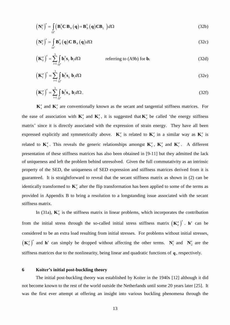
e
sK and e
tK are conventionally known as the secant and tangential stiffness matrices. For
the ease of association with e
sK and e
tK , it is suggested that e
eK be called ‘the energy stiffness
matrix’ since it is directly associated with the expression of strain energy. They have all been
expressed explicitly and symmetrically above. e
sK is related to e
eK in a similar way as e
tK is
related to e
sK . This reveals the generic relationships amongst e
eK , e
sK and e
tK . A different
presentation of these stiffness matrices has also been obtained in [9-11] but they admitted the lack
of uniqueness and left the problem behind unresolved. Given the full commutativity as an intrinsic
property of the SED, the uniqueness of SED expression and stiffness matrices derived from it is
guaranteed. It is straightforward to reveal that the secant stiffness matrix as shown in (2) can be
identically transformed to e
sK after the flip transformation has been applied to some of the terms as
provided in Appendix B to bring a resolution to a longstanding issue associated with the secant
stiffness matrix.
In (31a), 0
eK is the stiffness matrix in linear problems, which incorporates the contribution
from the initial stress through the so-called initial stress stiffness matrix 0
eK . e
h can be
considered to be an extra load resulting from initial stresses. For problems without initial stresses,
0
eK and e
h can simply be dropped without affecting the other terms. 1
eN and 2
eN are the
stiffness matrices due to the nonlinearity, being linear and quadratic functions of q , respectively.
6 Koiter’s initial post-buckling theory
The initial post-buckling theory was established by Koiter in the 1940s [12] although it did
not become known to the rest of the world outside the Netherlands until some 20 years later [25]. It
was the first ever attempt at offering an insight into various buckling phenomena through the
14
concept of stability of equilibrium states, in particular, those in the initial post-buckling regime.
Through this, the concept of imperfection sensitivity of a structure was quantitatively established
and directly associated with the stability of the initial post-buckling equilibrium state. The stability
of the initial post-buckling equilibrium state and the sensitivity of the buckling load to the initial
imperfection could all be described through two non-dimensional parameters, a and b, often termed
as initial post-buckling coefficients (IPBCs) [26]. Research activities on the theory peaked in the
1970s [26,27] when the development of commercial FEM codes was still in its infancy. Modern
mainstream commercial FEM codes have never managed to incorporate Koiter’s theory.
Buckling analysis is one of the basic modules in modern commercial FEM codes [1-3].
However, structural engineers and designers are very aware of the limitations of the predicted
buckling load. Structures could collapse at a much lower load level than the predicted buckling
load due to their imperfection sensitivity. As the buckling analysis alone is insufficient to provide
any information in this regard, investigations have been taken to the post-buckling regime which
could be traced as far back as to the 1940s [27] with intensified activities in the 1960s [28,29], to
name but a few. The outcomes of such efforts, whilst having enhanced the understanding of the
post-buckling deformation, proved to be a rather inefficient approach to understanding buckling
behaviour. A modern equivalent of such efforts is to analyse structures with artificially introduced
imperfections, often as an initial deflection taking the pattern of the buckling mode, taking
advantage of the computing power nowadays and the options available in mainstream FEM codes.
Such analyses are computationally expensive and time-consuming. A proper assessment will have
to involve separate runs having imperfections of either sense one at a time and they will have to be
run over a range of magnitudes of such artificially introduced imperfection in order to be
representative. This is often missing from such attempts. The computational cost could be
overwhelming, bearing in mind that each of such an analysis must be conducted as a nonlinear
problem. In most of such endeavours, the ultimate objective is in fact some assurance on the
predicted buckling load.
Much of the useful part of the outcomes of the above computationally expensive and time-
consuming exercises could have been condensed into the two IPBCs, a and b, if Koiter’s theory had
been adopted. Their evaluations involve little more than a conventional buckling analysis, typically
the extraction of the lowest order of eigenvalue, in terms of computational efforts. To be specific,
the evaluation of a requires no more information than has been made available after the buckling
analysis. That for b needs slightly more effort since one has to solve another specially formulated
stiffness equation to obtain the 2nd order of displacement perturbation. This is a linear problem.
Computationally, it is equivalent to a single iteration in a conventional incremental-iterative
nonlinear analysis. Koiter’s theory is called the initial post-buckling theory and it does produce a

15
prediction of the post-buckling deformation. However, it is meant to be applicable to the initial
phase of the post-buckling regime in an asymptotic sense. It is usually insufficient to offer
meaningful understanding of post-buckling deformation in a broad sense, if such information is
genuinely required. The true value of Koiter’s theory is to provide an efficient tool for designers
dealing with buckling as they will have much improved level of confidence on the buckling load
predicted if it is accompanied by IPBCs a and b. In this regard, through the development of the
theory in the 1970-80s, mostly by analytical means, a reasonable understanding has been achieved
in terms of their imperfection sensitivity of simple structures, such as plates and cylindrical shells.
However, modern structures tend to have intricate details, e.g. panels with hat-shaped stiffeners,
often involving the use of new materials, such as composites, and their imperfection sensitivity is
no longer obvious before an appropriate evaluation has been carried out.
In order to present this paper in self-contained form, the main procedure of Koiter’s theory
is provided briefly in its FEM presentation. With the FEM discretisation, after assembling all
elements involved in the structure, the total potential energy for a conservative elastic system can be
given as
1 2 3 4 q q q q q (33)
where the same q has been used for the nodal displacement vector for the whole structure without
being confused with its counterpart for an element. Having employed the fully commutative and
apparently symmetric SED to formulate element stiffness matrices as shown in the previous section,
the full commutativity of q is present in 2 , 3 and 4 for the structure. Equilibrium is defined
by the first variation of
1 11 21 31, , , 0 q q q q q q q q (34)
where the subscript rules for remain the same as for Q in previous sections as illustrated in (17)
and (18) in line with Koiter’s original notation [12].
As conventionally assumed, there exists a fundamental equilibrium path given as
0 0 q q satisfying 0 0 q 0 . (35)
where the load parameter and c the critical load. The critical condition for buckling is met as
increases from 0 to c , when the second variation as follows seizes to be positive definite, i.e.
2
11 111 0 211 0, , , , , 0 q q q q q q q q q (36)
whilst there exists a nontrivial displacement variation 1 q q that results in a zero value for the
second variation above, i.e.
11 1 111 0 1 211 0 1, , , , , 0 q q q q q q q q (37)
16
which gives the governing equation for the eigenvalue problem where the lowest eigenvalue
determines the magnitude of 0q at buckling, i.e. c , and eigenvector 1q provides the buckling
mode.
The classical buckling problem finishes at this point. However, structures tend to exhibit a
range of dramatically different behaviours. Some can support further loads after buckling whilst
others collapse long before the classical buckling load is reached. Koiter established [12,25] that
the different responses were directly related to the state of stability of the post-buckling equilibrium
path at the bifurcation point. If it were stable, the structure would be insensitive to the initial
imperfection and it could sustain higher levels of load without catastrophic collapse. Otherwise, the
structure would be sensitive to the initial imperfection and it would tend to collapse at a load
significantly lower than the predicted buckling load, depending on the magnitude of the initial
imperfection. In order to obtain the initial post-buckling path and to assess the stability of the
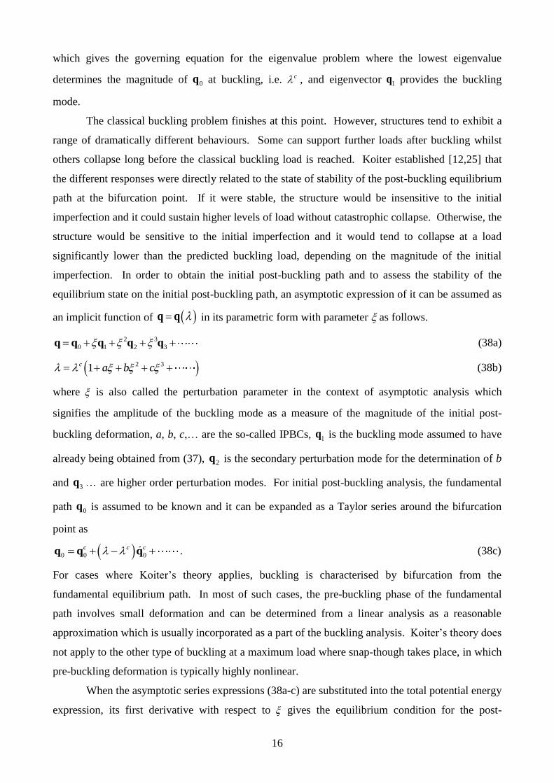
equilibrium state on the initial post-buckling path, an asymptotic expression of it can be assumed as
an implicit function of q q in its parametric form with parameter as follows.
2 3
0 1 2 3 q q q q q (38a)
2 31c a b c (38b)
where is also called the perturbation parameter in the context of asymptotic analysis which
signifies the amplitude of the buckling mode as a measure of the magnitude of the initial post-
buckling deformation, a, b, c,… are the so-called IPBCs, 1q is the buckling mode assumed to have
already being obtained from (37), 2q is the secondary perturbation mode for the determination of b
and 3q are higher order perturbation modes. For initial post-buckling analysis, the fundamental
path 0q is assumed to be known and it can be expanded as a Taylor series around the bifurcation
point as
0 0 0
c c c q q q . (38c)
For cases where Koiter’s theory applies, buckling is characterised by bifurcation from the
fundamental equilibrium path. In most of such cases, the pre-buckling phase of the fundamental
path involves small deformation and can be determined from a linear analysis as a reasonable
approximation which is usually incorporated as a part of the buckling analysis. Koiter’s theory does
not apply to the other type of buckling at a maximum load where snap-though takes place, in which
pre-buckling deformation is typically highly nonlinear.
When the asymptotic series expressions (38a-c) are substituted into the total potential energy
expression, its first derivative with respect to gives the equilibrium condition for the post-
17
buckling path and can be considered as an implicit function . If a and b in (38b) are
considered as the 1st and 2nd order of derivatives of with respective to at 0 and hence
c , their expressions can be obtained as follows.
3 1 13 0 1
12 0 1 112 0 0 1
,3
2 , , ,
c
c c c ca
q q q
q q q q q (39)
4 1 2 2 12 0 2 22 0 2
12 0 1 112 0 0 1
, ,20
, , ,
c c
c c c cb a
q q q q q q
q q q q q (40)
In most practical analyses, determination of a and b is sufficient. As established in Koiter’s theory,
the most important characteristics of the initial post-buckling behaviour can be determined using
only these constants, provided that they do not vanish simultaneously.
If 0a , the initial post-buckling path given in (38b) can be truncated at the first order of
the asymptotic series as an approximation and one does not even need to evaluate b as it contributes
only an asymptotically higher order term. In this case, an asymmetric bifurcation is expected which
predicts an unstable initial post-buckling behaviour in general and leads to imperfection sensitivity.
Given the asymmetric nature of the bifurcation, if the structure is sensitive to an imperfection of one
sense, e.g. positive, it is insensitive to the same imperfection of the other sense, i.e. negative. This
is why if one adopts the nonlinear post-buckling analysis approach, imperfections of both senses
must be assessed separately to form a complete view.
When a=0, one has to proceed to the second order perturbation. If 0b , function (38b) can
be truncated at the second order term for initial post-buckling behaviour leading to a symmetric
bifurcation. In order to evaluate b, the second order displacement perturbation 2q is required. The
governing equation can be obtained from the second order terms of in the asymptotically
expanded total potential energy as [12,25]
11 2 111 0 2 121 0 2 12 1 112 0 1, , , , , , , , q q q q q q q q q q q q q (41)
subject to an orthogonality condition between 1q and 2q as
11 0 1 2 1111 0 0 1 2, , , , , 0c c c q q q q q q q . (42)
Higher orders of perturbation could be made in theory in the case that b vanishes but this situation
rarely arise in practice.
Koiter’s theory has been summarised as above. However, it has not been implemented in
any mainstream commercial FEM code. In fact, there has been no lack of desire to achieve this,
early attempts could be traced back to the 1970s [13, 14] and numerous more recent efforts could be
found including those in [16-23]. The development of the FEM implementation of Koiter’s theory

18
has suffered from a number of key obstacles. One of them was referred to as the ‘locking’
phenomenon as originally defined in [31]. It will be resolved as one of the main outcomes of the
present paper. The remaining obstacles have also been resolved by the present authors who plan to
present them soon in subsequent publications.
Making use of the SED and FEM formulation as presented in previous section, key
governing equations as presented above can be expressed in the FEM context as follow.
0 1 2
1 1 1
2 6 12
q K N N q q F cf. (33) (43)
0 1 2
1 10
2 3
K N N q F cf. (34) (44)
0 1 2 1 K N N q 0 cf. (37) (45)
1 1 1 1 1 2 1 0
1 1 1 0 1 2 0 0
21
2 2
c
c c c ca
q N q q q N q q
q N q q q N q q
cf. (39) (46)
1 2 1 1 2 0 1 0 2 0 2
1 1 1 0 1 2 0 0
61
3 2
c c
c c c cb
q N q q q K N q N q q
q N q q q N q q
cf. (40) (47)
0 1 2 2 1 1 1 2 1 0
1
2
c K N N q N q q N q q cf. (41) (48)
1 1 0 11 0 0 2, 0T c c c q N q N q q q cf. (42) (49)
where F is the external loading vector whilst various symbols associated with the FEM formulation
are inherited from the previous section in a straightforward manner except that they have been
assembled from all elements involved in the structure.
The expressions of a and b above were obtained as early as in 1971 [13]. However, they
have remained unimplemented because the nonlinear stiffness matrices 1N and 2N have been a
‘symbolism’ as referred to in the first edition of [4]. In obtaining them in [13], the full
commutativity of various displacements within each of the terms appearing in the expressions had
been taken for granted, which did not stand scrutiny if one wished to adopt it in a commercial code.
Based on the full commutativity and the apparent symmetry as established earlier in this
paper, all expressions now are not only well-defined and explicit but also proven to be practically
effective in applications as will be demonstrated in the next section.
In the literature, most attempts of evaluating the IPBCs a and b through FEM have
employed the expressions as provided in Appendix C as an alternative. They are mathematically
equivalent to (39) and (40), respectively. However, the equivalence for b was greatly compromised
numerically when implemented through FEM, as the two terms in the numerator of (C-2) are of

19
opposite senses whilst having similar magnitude. The sum is often one or more orders of
magnitude smaller, resulting in the so-called ‘locking’ phenomenon [31]. The fact that it has never
appeared in analytical solutions [15] suggests that it is a numerical problem associated with
accuracy. The underlying reason was in fact the generic shortcoming of FEM in which stresses
obtained are inherently found to a lower order of accuracy. As expression (C-2) involves stresses
explicitly, the accuracy of the results would have to rely on mesh refinement. Such mesh sensitivity
for this particular problem has been well-observed and documented in the literature, e.g. [16-23].
The consequence is that a much more refined mesh would be required for initial post-buckling
analysis than that which would usually be sufficient to deliver satisfactory buckling analysis. This
would undermine the practical usefulness of an FEM code. To improve the accuracy in order to
avoid the mesh sensitivity, specially formulated finite elements have been adopted using
unconventional shape functions, e.g. those having higher orders of continuity [16]. Neither
enduring the mesh sensitivity nor employing specially formulated elements is an attractive property
to FEM code developers. It was undoubtedly one of the major reasons why the theory has never
been incorporated in any mainstream FEM code.
Since (C-2) on longer relies on stresses, one can expect (47) to offer improved performance.
This will be demonstrated in the next section through example applications. It will be shown that it
has in fact removed the mesh sensitivity completely without having to use a specially formulated
element.
7 Numerical examples
To demonstrate the advantages of the formulation as presented in Section 6, it is applied
here to the plates presented in [16]. The formulation can be simplified accordingly for plates and
shells where all higher order terms of in-plane displacements can be neglected, as has been
conventionally performed in [6-8]. The plate is considered to take a range of aspect ratios and is
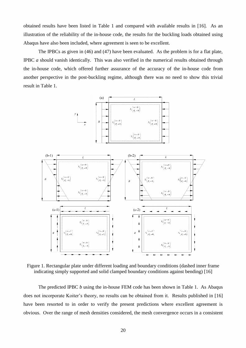
assumed to be simply supported (a), (b-1) and (c-1) or clamped (b-2) and (c-2) with in-plane
constraints as specified in Figure 1. It is subjected to a number of loading conditions, viz. (a)
uniaxial compression, (b) pure in-plane bending and (c) pure shear, as illustrated in Figure 1. The
Young’s modulus of the material of the plate is 210 GPaE and its Poisson’s ratio 0.3v . The
thickness of the plate is 1t mm .
Given the absence of Koiter’s theory from any mainstream commercial FEM code, the
present analyses were conducted using an in-house developed FEM code employing the 3D
degenerated 8-noded shell element with reduced integration [4,5]. Prior to the applications shown
in this paper, the code had been extensively verified against various sources, including analytical
solutions wherever available and the results obtained from Abaqus. For the present application, the
20
obtained results have been listed in Table 1 and compared with available results in [16]. As an
illustration of the reliability of the in-house code, the results for the buckling loads obtained using
Abaqus have also been included, where agreement is seen to be excellent.
The IPBCs as given in (46) and (47) have been evaluated. As the problem is for a flat plate,
IPBC a should vanish identically. This was also verified in the numerical results obtained through
the in-house code, which offered further assurance of the accuracy of the in-house code from
another perspective in the post-buckling regime, although there was no need to show this trivial
result in Table 1.
Figure 1. Rectangular plate under different loading and boundary conditions (dashed inner frame
indicating simply supported and solid clamped boundary conditions against bending) [16]
The predicted IPBC b using the in-house FEM code has been shown in Table 1. As Abaqus
does not incorporate Koiter’s theory, no results can be obtained from it. Results published in [16]
have been resorted to in order to verify the present predictions where excellent agreement is
obvious. Over the range of mesh densities considered, the mesh convergence occurs in a consistent

21
way between the buckling load and IPBC b, i.e. a mesh good enough for buckling analysis is also
good enough for initial post-buckling analysis.
Table 1. Initial post-buckling coefficient of simply supported rectangular plate
Case Mesh
Normalised buckling load
2 2 2 312 1 cB Et IPBC
b
Partitions of b such
that b=b1b2
b1 b2 Ref.[16] Abaqus Present Ref.[16] Present
(a)
L/B=3
217 4.033 3.969 3.968 0.2203 0.2108 1.7716 1.5608
3311 4.014 3.974 3.974 0.2213 0.2190 1.9215 1.7025
4915 4.007 3.974 3.974 0.2217 0.2149 1.8838 1.6689
(b-1)
L/B=1
99 26.18 25.49 25.31 0.2236 0.2160 2.0664 1.8504
1515 25.76 25.32 25.25 0.2252 0.2156 2.0441 1.8285
2525 25.61 25.27 25.25 0.2194 0.2097 2.0129 1.8032
3333 25.58 25.26 25.25 0.2193 0.2104 2.0257 1.8153
(b-2)
L/B=1
99 53.49 48.90 48.44 0.3400 0.2838 1.3404 1.0566
1515 49.74 47.71 47.55 0.2978 0.2926 1.3913 1.0987
2525 48.46 47.55 47.50 0.2978 0.2806 1.3352 1.0546
3333 48.16 47.53 47.50 0.2924 0.2854 1.3569 1.0715
(c-1)
L/B=2
157 6.777 6.537 6.537 0.07297 0.07305 1.2558 1.1828
2511 6.639 6.522 6.523 0.07174 0.07273 1.2635 1.1908
3317 6.587 6.521 6.521 0.07164 0.07226 1.2758 1.2036
(c-2)
L/B=2
157 11.41 10.37 10.37 0.1566 0.1357 1.3057 1.1700
2511 10.67 10.23 10.23 0.1383 0.1330 1.2982 1.1652
3317 10.42 10.22 10.22 0.1340 0.1326 1.2924 1.1598
The agreements with [16] and Abaqus verify the correctness of the formulation and the
implementation. A much more important aspect is that the present analysis employs a conventional
type of finite element, viz. 3D degenerated 8-noded shell with reduced integration, available
commonly in commercial FEM codes, whilst that in [16] was based on specially formulated finite
elements with a higher order of continuity which is unavailable in any mainstream commercial code.
It should be pointed out that an analytical solution for b is available in [27] for a problem
corresponding to Case (a), given as
231 0.34125
8b
(50)
which is significantly different from what was obtained in [16] as well as the present prediction. It
is most disturbing to enquire why the disparity has never been flagged up and explained
appropriately. There appeared to be reluctance in the literature, e.g. [20], to refer to Case (a). It
would be extremely negative for any serious developer of FEM code considering adaption of
Koiter’s theory, if such the discrepancy were left unaddressed. The authors of this paper have
22
identified the source of the problem and resolved it. Since it is not simply a numerical error and
takes a considerable elaboration on both numerical and analytical sides in order to clarify the
position, it will have to be presented in a subsequent publication. For readers’ assurance, the result
as presented in Table 1 is correct for the problem as defined in Figure 1(a), which is however subtly
different from that solved analytically in [27].
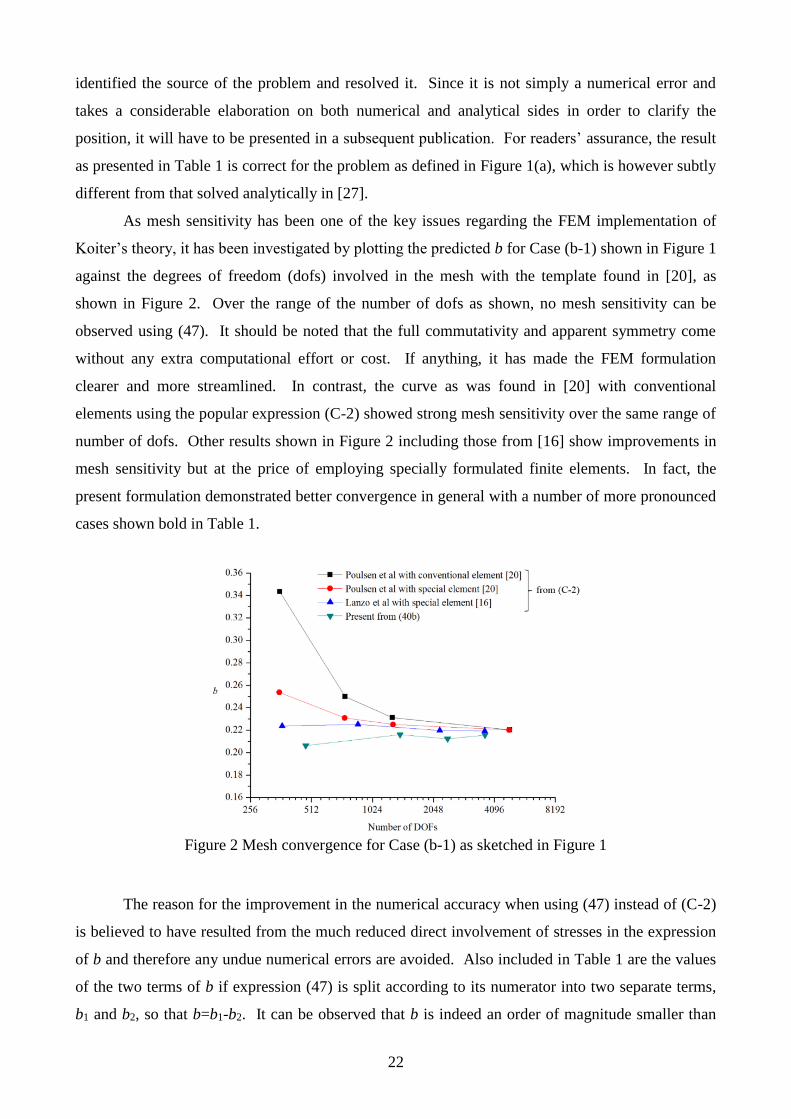
As mesh sensitivity has been one of the key issues regarding the FEM implementation of
Koiter’s theory, it has been investigated by plotting the predicted b for Case (b-1) shown in Figure 1
against the degrees of freedom (dofs) involved in the mesh with the template found in [20], as
shown in Figure 2. Over the range of the number of dofs as shown, no mesh sensitivity can be
observed using (47). It should be noted that the full commutativity and apparent symmetry come
without any extra computational effort or cost. If anything, it has made the FEM formulation
clearer and more streamlined. In contrast, the curve as was found in [20] with conventional
elements using the popular expression (C-2) showed strong mesh sensitivity over the same range of
number of dofs. Other results shown in Figure 2 including those from [16] show improvements in
mesh sensitivity but at the price of employing specially formulated finite elements. In fact, the
present formulation demonstrated better convergence in general with a number of more pronounced
cases shown bold in Table 1.
Figure 2 Mesh convergence for Case (b-1) as sketched in Figure 1
The reason for the improvement in the numerical accuracy when using (47) instead of (C-2)
is believed to have resulted from the much reduced direct involvement of stresses in the expression
of b and therefore any undue numerical errors are avoided. Also included in Table 1 are the values
of the two terms of b if expression (47) is split according to its numerator into two separate terms,
b1 and b2, so that b=b1-b2. It can be observed that b is indeed an order of magnitude smaller than
23
either b1 or b2 and hence ‘locking’ is likely [16,17], especially if the terms involved could not be
evaluated sufficiently accurately. However, having reduced the direct involvement of stresses in
these expressions, numerical errors due to FEM should have been reduced in comparison with that
evaluated using (C-2). The freedom from mesh sensitivity in the present results is therefore by no
accident.
Use of (47) brings forward a satisfactory solution and locking does not appear whilst using a
conventional type of C0 element. This has been achieved based on the N-notation which was not
possible practically previously. With the fully commutative and apparently symmetric SED, the N-
notation is now fully established. This should open the gate for Koiter’s theory to be incorporated
in mainstream commercial FEM codes.
8 Conclusions
In this paper, the concept of full commutativity of displacements in the expressions for the
strain energy density within the geometrically nonlinear problem has been introduced for the first
time, and established firmly such that full commutativity can now be identified as an intrinsic
property of the SED.
When this fully commutative SED is employed in the formulation of the FEM, as a direct
application, all relevant stiffness matrices in the so-called N-notation can be obtained uniquely. In
order for them to be expressed explicitly, the SED also needs to be put into an apparently symmetric
form by applying the mathematically identical flip transformation to some of the terms of the SED,
as has also been established in this paper. The stiffness matrices thus obtained can then be used to
construct the strain energy, equilibrium equation and the incremental equilibrium equation in a
consistent manner. The N-notation FEM formulation has thus been fully and rigorously established.
Prior to this, the N-notation formulation has remained as a symbolism, particularly within the FEM
implementation of Koiter’s theory. Without a functional N-notation formulation, the option for the
FEM implementation of Koiter’s theory is through the B-notation instead, which has suffered from
the well-known mesh sensitivity issue in the evaluation of the IPBC b unless some unconventional
types of elements have been employed. With the expression of b in N-notation, the mesh sensitivity
issue has been resolved naturally whilst using a conventional type of element. There will be no
need either to employ specially formulated elements or to endure the inconvenience of mesh
sensitivity, as has been demonstrated in the present paper. The unavailability of Koiter’s theory
from commercial FEM codes is a missed opportunity for structural designer and engineers to
improve dramatically the confidence in the predicted load carrying capacity of structures when
designing against buckling. Using any existing commercial FEM code, it is easy to predict the
buckling load but difficult to place confidence on it; Koiter’s theory would overcome this problem.

24
The most important contribution of this paper is to pave a way for the wide adoption of Koiter’s
theory in mainstream FEM codes.
Acknowledgement
The work presented in this paper was sponsored by AVIC Aircraft Strength Research
Institute, China, under contract no. 110961. The first author wishes to express his gratitude to
Professors John Hutchinson and Robert Cook for their comments on earlier versions of the
manuscript of this paper in various aspects. The second author would like to acknowledge the
scholarship awarded by China Scholarship Council. The authors are also obliged to Professor
Arthur Jones for proof reading the manuscript and valuable comments.
References
[1] Abaqus, Abaqus 2016 Analysis User’s Guide, Dassault Systèmes, 2015
[2] Nastran, Nastran 2016 Nonlinear User’s Guide, MSC, Newport Beach, CA, 2016
[3] Ansys, Ansys Mechanical User’s Guide, ANSYS, Canonsburg, PA, 2013
[4] Cook R.D., Plesha M.E., Malkus D.S., Witt R. (2001) Concepts and Applications of Finite
Element Analysis, 4th edition, Wiley, London
[5] Zienkiewicz O.C., Taylor R.L. (2000) The Finite Element Method, 5th edition, Vol.2, Arnold,
London
[6] Bonet J., Wood R.D. (1997) Nonlinear Continuum Mechanics for Finite Element Analysis,
Cambridge University Press, Cambridge
[7] Crisfield M.A. (1997) Nonlinear Finite Element Analysis of Solids and Structures, Vol. 1&2,
Wiley, Chichester
[8] Fung Y.C., Tong P. (2001) Classical and Computational Solid Mechanics, World Scientific,
London
[9] Wood R.D., Schrefler B. (1978) Geometrically non-linear analysis – A correlation of finite
element notations. International Journal for Numerical Methods in Engineering; 12:635-642
[10] Rajasekaran S., Murray D.W. (1973) Incremental finite element matrices. Journal of the
Structural Division; 99: 2423-2438
[11] Felippa C.A. (1974) discussion on [9]; 100: 2521-2523
[12] Koiter W.T. (1945) ‘On the Stability of Elastic Equilibrium’, Thesis, Delft University,
Amesterdam, 1945 (in Dutch). English translation: Stanford University (1967), NASA TT
F-10, 833; also Dept Aero Astro Report AD 704124 (1970)/Airforce Flight Dynamics Lab
Report TR-70-25
[13] Haftka R., Mallet R., Nachbar W. (1971) ‘Adaptation of Koiter’s method to finite element
analysis of snap-through buckling behaviour’, International Journal of Solids and Structures,
7:1427-47
[14] Gallagher R.H., Lien S., Mau S.T. (1973) A procedure for finite element plate and shell pre-
and post-buckling analysis. Proceedings of the Third Conference on Matrix Methods in
Structural Mechanics; 857-880

25
[15] Budiansky B., Hutchinson J.W. (1964) ‘Dynamic buckling of imperfection-sensitive
structures’, Proceedings of the XI International Congress of Applied Mechanics, Berlin,
pp636-651
[16] Lanzo A.D., Garcea G., Casciaro R. (1995) ‘Asymptotic post-buckling analysis of
rectangular plates by hc finite elements’, International Journal of Numerical Methods in
Engineering, 38:2325-2345
[17] Casciaro R., Garcea G., Attanasio G., Giordano F. (1997) ‘Perturbation approach to elastic
post-buckling analysis’, Computers and Structures, 66:585–595
[18] Garcea G., Salerno G., Casciaro R. (1999) ‘Extrapolation locking and its sanitisation in
Koiter’s asymptotic analysis’, Computer Methods in Applied Mechanics and Engineering,
180:137–167
[19] Garcea G., Madeo A., Zagari G., Casciaro. (2009) ‘Asymptotic post-buckling FEM analysis
using corotational formulation’, International Journal of Solids and Structures, 46:377–397
[20] Poulsen P.N., Damkilde L. (1998), ‘Direct Determination of asymptotic structural
postbuckling behaviour by the finite element method’, International Journal for Numerical
Methods in Engineering, 42:685-702
[21] Zagari G., Madeo A., Casciaro R., de Miranda S., Ubertini F. (2012) ‘Koiter analysis of
folded structures using a corotational approach’, International Journal of Solids and
Structures, 50:755–765
[22] Magisano D., Leonetti L., Carcea G. (2016) ‘Koiter asymptotic analysis of multilayered
composite structures using mixed solid-shell finite elements’, Composite Structures,
154:296–308
[23] Garcea G., Liguori F., Leonetti L., Magisano D., Madeo A. (2017) ‘Accurate and efficient a-
posteriori account of geometrical imperfections in Koiter finite element analysis’,
International Journal for Numerical methods in Engineering, doi: 10.1002/nme.5550
[24] Korn GA, Korn TM. (2000) Mathematical Handbook for Scientists and Engineers, 2nd
edition, Dover Publications, New York
[25] Koiter W.T. (1963) ‘Elastic stability and post-buckling behavior’, Proceedings of
Symposium on Nonlinear Problems, University of Wisconsin Press, Madison, pp257–275
[26] Hutchinson J.W. and Koiter W.T. (1970) ‘Postbuckling theory’, Appl. Mech. Rev. 23:1353-
1362
[27] Budiansky B. (1974) ‘Theory of buckling and postbuckling behaviour of elastic structures’,
Advances in Applied Mechanics, 114:1–65
[28] Von Karman T., Tsien, H.S. (1941) ‘the buckling of thin cylindrical shells under axial
compression’, Journal of the Aeronautical Sciences, 8:303-312
[29] Hoff, N.J., Madsen, W.A. Mayers, J. (1966) ‘Postbuckling equilibrium of axially
compressed circular cylindrical shells’, AIAA Journal, 4:126-133
[30] Almroth, B.O. (1963) ‘Postbuckling behaviour of axially compressed circular cylinders’,
AIAA Journal, 1: 630-633
[31] Byskov E. (1989), ‘Smooth postbuckling stresses by a modified finite element method’,
International Journal for Numerical Methods in Engineering, 28:2877-2888.

26
Appendix A Basic equations and notations
Basic notations involved in this paper are defined as follows. For a linearly elastic
continuum as dealt with in this paper, the strain energy density U exists and it can be expressed as
1
2IU u ε σ ε σ (A-1)
where is the Green strain, Iσ the initial Cauchy stress and the second Piola-Kirchhoff stress [8].
L N ε ε ε , L Lε u , 1
2N N ε u u (A-2)
where u v w
u is the displacement field, and
0 0
0 0
0 0
,
0
0
0
L
x
y
z
z y
z x
y x
N
u v w
x x x x x x
u v w
y y y y y y
u v w
z z z z z z
u u v v w w
y z z y y z z y y z z y
u u v v w w
z x x z z x x z z x x z
u u v v w w
x y y x x y y x x y y
u
x
(A-3)
where operator L and N u are both defined according to the Green strain with the latter
containing homogeneous linear expressions of the derivatives of u . These operators apply to the
displacement field on its right, e.g. L u and N u u . Transposing these expressions reverses the
sequence of these operators, e.g. L
u and N
u u . Given the expression of N u , u and u
in N u u are commutative, i.e. N N u u u u .
Under the assumption of linear elasticity, the constitutive relationship can be given as
I I L N I L N σ σ Cε σ Cε Cε σ σ σ (A-4)
where C is the material stiffness, Lσ and Nσ are linear and quadratic parts of the second Piola-
Kirchhoff stress in their contracted form, with Nσ representing the effects of geometrical
nonlinearity. In some parts of the derivation involved in the paper, the matrix form these stresses
are required and they will be denoted as s , Is , Ls and Ns , respectively.
Having introduced the notations above, (A-1) can be partitioned according to the orders of
displacements as follows.
1 2 3 4U U U U U (A-5a)
where 1 L I L IU ε σ u σ (A-5b)
27
2
1 1 1
2 2 2N I L L N I L LU ε σ ε ε u u σ u C uC (A-5c)
3
1 1
2 2L N N L L N L NU ε C ε ε Cε ε C ε u C u u (A-5d)
4
1 1
2 8N N N NU ε C ε u u C u u . (A-5e)
The subscripts to various terms of U above indicate the orders of power in displacement. Each of
1U to 4U is a homogeneous function of u and hence can be expressed as a linear, quadratic, cubic
or quartic form of u as in (A-5b) to (A5-e), respectively. Geometrical nonlinearity is brought into
the problem through 3U and 4U which are often referred to as higher order terms whilst 1U and
2U pertain to the conventional linear problem.
To derive the stiffness matrices of a finite element for the geometrically nonlinear problem
the displacement field in a finite element can be discretised as follows.
u Aq (A-6)
where q is the nodal displacement vector for the element corresponding to the displacement field u
and A is the displacement interpolation matrix which is formed from shape functions.
L Lε B q , 1
2N Nε B q q (A-7)
where L LB A (A-8a)
N N N B q u A q A with N Aq denoted later as N q (A-8b)
LB is independent of q , whilst all the elements of NB are homogeneous linear expressions of q ,
which represents the effects of geometrical nonlinearity in the kinematic equation. Matrices LB
and NB may vary with the type of element, including truss, membrane and brick continuum
elements and beam, plate and shell structural elements. Following an argument that was made
earlier, q and q involved in N B q q are commutative, i.e. N N B q q B q q .
Discretising the term in 11 associated with SI as in (22a) leads to
3
1
I i I i
i
u S u q b s b q (A9a)
where i ib A . (A9b)
Similarly, those in 111 and 1111 associated with SL and S11 as in (22b-c) are discretised to
3
1
L i L i
i
u S q u q b s u b q with L L L
s q s Aq s u (A10)
28
3
11 11
1
, ,i i
i
u S u u u q b s u u b q with 11 11, , s q q s u u (A11)
whilst
3
11
1
1,
2N i i
i
u S u u q b s u u b q with N Ns q s u (A12)
as a part of (25c) after discretisation.
Appendix B Derivation of the flip transformation and an example of its application
N I Ix Iy Iz
Iyz Izx Ixy
u u u u u u
x x y y z z
u u u u u u u u u u u u
y z y z z x z x x y x y
u u
Ix Ixy Ixz Ix Ixy Ixz
Ixy Iy Iyz Ixy Iy Iyz
Ixz Iyz Iz Ixz Iyz Iz
u u v v
x x x x
u u v v
y y y y
u u v v
z z z z
Ix Ixy Ixz
Ixy Iy Iyz
Ixz Iyz Iz
w w
x x
w w
y y
w w
z z
T T T
T T T T T T
1 1 2 2 3 3
T
I I I
I I I
I
u u v v w w
s s s
u s u u s u u s u
u S u
(B1)
where IS and
i have been given in (19b) and (19c). Applying the flip transformation to
discretised energy terms, e.g. those involved in (2), one can readily recover the symmetry of the
secant stiffness matrix as in (2).
0 1 2
3 3
0 1 2
1 1
1 1
2 2
1 1 1 1
2 3 2 6
1 1 1 1
2 3 2 3
e
e
e e
e
L L L N N L N N
e ee q q
N L N N
e ee q q
i L i i N i
i i
U d
d
d d
q B CB B CB q B q CB B q CB q q
q K N N B q CB B q CB q q
q K N N b s b b s b
0 1 2 1 2
0 1 2
1 1 1 1
2 3 2 3
1 1
2 3
e e e ee q q
e e e e
s
q
q K N N K K q
q K N N q q K q
(B2)
where various stiffness matrices have been given in (30) to (32). Without making the relevant
expression apparently symmetric through the flip transformation, the secant stiffness matrix cannot
be obtained explicitly.
29
Appendix C Alternative expressions for the IPBCs and their drawback
Alternative expressions of the IPBCs a and b were obtained in [15]. Presented in the
notations of this paper, they were expressed as follows.
T
1 1 1
0 1 1
3
2
N
cc
N
d
ad
σ q q
σ q q
(C-1)
T T
2 1 1 1 1 2
0 1 1
21
N N
cc
N
d
bd
σ q q σ q q
σ q q
(C-2)
where 1N q is defined in the same way as (A-8b) but with q replaced by 1q , 0
cσ the stress state on
the fundamental equilibrium path at the point of buckling, and 1σ and 2σ are the first and second
order perturbation stresses defined as follows (to be distinguished from Lσ and
Nσ ).
0 0 0
1
2
c c c
L N
σ C q q
(C-3)
1 0 1
c
L N σ C q q (C-4)
2 0 2 1 1
1
2
c
L N N
σ C q q q q . (C-5)