impacts of variability and uncertainty in solar photovoltaic generation … · 2013-10-07 ·...

NREL is a national laboratory of the U.S. Department of Energy, Office of Energy Efficiency & Renewable Energy, operated by the Alliance for Sustainable Energy, LLC.

Contract No. DE-AC36-08GO28308

Impacts of Variability and Uncertainty in Solar Photovoltaic Generation at Multiple Timescales E. Ela, V. Diakov, E. Ibanez, and M. Heaney National Renewable Energy Laboratory

Technical Report NREL/TP-5500-58274 May 2013

NREL is a national laboratory of the U.S. Department of Energy, Office of Energy Efficiency & Renewable Energy, operated by the Alliance for Sustainable Energy, LLC.

National Renewable Energy Laboratory 15013 Denver West Parkway Golden, Colorado 80401 303-275-3000 • www.nrel.gov

Contract No. DE-AC36-08GO28308

Impacts of Variability and Uncertainty in Solar Photovoltaic Generation at Multiple Timescales E. Ela, V. Diakov, E. Ibanez, and M. Heaney National Renewable Energy Laboratory

Prepared under Task No. SS13.3030

Technical Report NREL/TP-5500-58274 May 2013

NOTICE

This report was prepared as an account of work sponsored by an agency of the United States government. Neither the United States government nor any agency thereof, nor any of their employees, makes any warranty, express or implied, or assumes any legal liability or responsibility for the accuracy, completeness, or usefulness of any information, apparatus, product, or process disclosed, or represents that its use would not infringe privately owned rights. Reference herein to any specific commercial product, process, or service by trade name, trademark, manufacturer, or otherwise does not necessarily constitute or imply its endorsement, recommendation, or favoring by the United States government or any agency thereof. The views and opinions of authors expressed herein do not necessarily state or reflect those of the United States government or any agency thereof.

Available electronically at http://www.osti.gov/bridge

Available for a processing fee to U.S. Department of Energy and its contractors, in paper, from:

U.S. Department of Energy Office of Scientific and Technical Information P.O. Box 62 Oak Ridge, TN 37831-0062 phone: 865.576.8401 fax: 865.576.5728 email: mailto:[email protected]

Available for sale to the public, in paper, from:

U.S. Department of Commerce National Technical Information Service 5285 Port Royal Road Springfield, VA 22161 phone: 800.553.6847 fax: 703.605.6900 email: [email protected] online ordering: http://www.ntis.gov/help/ordermethods.aspx

Cover Photos: (left to right) PIX 16416, PIX 17423, PIX 16560, PIX 17613, PIX 17436, PIX 17721

Printed on paper containing at least 50% wastepaper, including 10% post consumer waste.

http://www.osti.gov/bridge

mailto:[email protected]

mailto:[email protected]

http://www.ntis.gov/help/ordermethods.aspx

iii

List of Acronyms AACEE absolute ACE in energy ACE area control error AGC automatic generation control APS Arizona Public Service CPS1 and CPS2 control performance standards (NERC) CSP concentrating solar power DASCUC day-ahead security-constrained unit commitment FESTIV Flexible Scheduling Tool for Integrating VG MAE mean absolute error NERC North American Electric Reliability Corporation PV photovoltaic RPU reserve pickup RTSCUC real-time security-constrained unit commitment RTSCED real-time security-constrained economic dispatch SCUC security-constrained unit commitment SCED security-constrained economic dispatch TEPPC Transmission Expansion Planning Policy

Committee (WECC) VG variable generation WECC Western Electricity Coordinating Council WWSIS-2 Western Wind and Solar Integration Study Phase 2

iv

Executive Summary This study investigates the effects of photovoltaic (PV) solar power variability and forecast uncertainty on electric power grid operation in the Arizona Public Service system. Both variability and uncertainty can create challenges for grid operators when balancing electricity generation with demand while obeying power system constraints and maintaining the lowest possible costs. Typically, studies of wind and solar variability are restricted to one time resolution. In this study, we analyze variability and uncertainty across several timescales, similar to the way power system operators manage load uncertainty. Our results aim to help grid operators prepare for increases in PV generation share and improve system reliability when integrating PV generation. We explore different mitigation strategies and methods to more reliably and efficiently integrate solar power.

This study is a follow on to the Western Wind and Solar Integration Study Phase 2. The APS balancing area within the Western Interconnection is studied in a high-load, high-PV, 5-day period during summer, as projected to the year 2020, at a 1-minute time-sampling frequency. We use the Flexible Scheduling Tool for Integrating Variable Generation (FESTIV). FESTIV integrates security-constrained unit commitment, security-constrained economic dispatch, and automatic generation control in one model. This allows multiple timescales to be studied and accounts for intertemporal coupling between them. FESTIV attempts to realistically simulate how most systems schedule generation in actual operation.

We find the following:

• The short-term forecast uncertainty increases the imbalance while having little impact on operating costs.

• The variability of solar power in itself without real-time uncertainty (i.e., with perfect hourly forecast) has little impact on imbalance and can actually improve certain imbalance effects.

• Power system operator intervention can mitigate some of the variability as well as uncertainty impacts while increasing operating costs.

• An improved day-ahead PV forecast reduces production costs with little effect on load-generation imbalance.

• A faster (5-minute versus 1-hour intervals) dispatch frequency has the advantage of a shorter forecast time horizon, so that imbalances can be corrected more often through dispatch instead of through limited automatic generation control resources. This has the effect of reducing both the imbalance and the system operating costs.

• Increasing regulation reserves to compensate for PV generation uncertainty improves system balance while raising production costs.

v

Table of Contents Introduction ................................................................................................................................................. 1 Flexible Scheduling Tool for Integrating Variable Generation ............................................................... 5 System Description ..................................................................................................................................... 9 The Impacts of Photovoltaic Variability and Uncertainty ..................................................................... 12 Imbalance Reduction Strategies ............................................................................................................. 19

Operator Action .................................................................................................................................... 19 Improved Day-Ahead Forecasts ........................................................................................................... 20 Increased Dispatch Frequency .............................................................................................................. 20 Regulation Reserve Increase ................................................................................................................ 22

Conclusion ................................................................................................................................................. 24 References ................................................................................................................................................. 27 Appendix A: Load and Interchange ........................................................................................................ 29 Appendix B: Day-Ahead Photovoltaic Forecast and Actual Photovoltaic Generation ...................... 30 Appendix C: Area Control Error Charts (Case 1–Case 7 in Order) ...................................................... 31

vi

List of Figures Figure 1. Depiction of variability and uncertainty ........................................................................................ 1 Figure 2. Operating reserve categorization [4] ............................................................................................. 3 Figure 3. Example of wind’s uncertainty and variability impacts on regulating reserve .............................. 4 Figure 4. Imbalance and regulating reserve needs resulting from variability and uncertainty ..................... 4 Figure 5. Flow diagram for FESTIV. Solid lines represent process flow, and dashed lines represent data

flow. ......................................................................................................................................... 5 Figure 6. Timeline for DASCUC, RTSCUC, RTSCED, and AGC in FESTIV ........................................... 7 Figure 7. Solar and Wind placements for the High Mix Scenario. (Yellow – PV, Orange – CSP, Green –

Wind). ...................................................................................................................................... 9 Figure 8. APS load and renewable generation as projected for a 5-day period from July 24 to July 28,

2020 ........................................................................................................................................ 10 Figure 9. ACE 1-day simulation. Perfect PV forecasts are used in the real-time simulation. .................... 13 Figure 10. ACE averaged over rolling 10-minute periods for 1-day simulation. Perfect forecasts are used

in the real-time simulation. .................................................................................................... 14 Figure 11. Generation for 1-day perfect forecast ........................................................................................ 15 Figure 12. Total generation and load for 5-day perfect forecast base case ................................................. 16 Figure 13. Regulation reserve requirements for Cases 1–6 (1% load) and Case 7 (WWSIS-2 [18]) ......... 22 Figure 14. CPS2 scores and production costs for all PV cases ................................................................... 25

List of Tables Table 1. Typical Timing Parameters ............................................................................................................. 7 Table 2. APS Generation Capacity (2020 Projection) .................................................................................. 9 Table 3. Assumptions Made in Simulations ............................................................................................... 11 Table 4. Forecast Performance for 5-Day Period Using Persistence (Wind) and Persistent Cloudiness (PV)

for 60-Minute RTSCED 5-Day Period .................................................................................. 17 Table 5. Comparison of Variability and Uncertainty Impacts .................................................................... 18 Table 6. Utilization of Operator Action Using RPU ................................................................................... 19 Table 7. Day-Ahead Forecast Performance for 5-Day Period for DASCUC ............................................. 20 Table 8. Day-Ahead Uncertainty Impact Improvements ............................................................................ 20 Table 9. Forecast Performance for 5-Day Period Using Persistence (Wind) and Persistent Cloudiness (PV)

for 60-Minute RTSCED 5-Day Period .................................................................................. 21 Table 10. Impact of 5-Minute Dispatch ...................................................................................................... 21 Table 11. Impact of Increased Regulation Requirements ........................................................................... 23 Table 12. Case Comparisons ....................................................................................................................... 24

1

Introduction Renewable power generation has seen a tremendous growth in recent years because it has environmental benefits and zero fuel costs. Unlike many conventional generation sources, however, many renewable resources, including wind power and photovoltaic (PV) solar power are considered variable generation (VG). They have a maximum generation limit that changes with time (variability) and this limit is not known with perfect accuracy (uncertainty). Variability of VG occurs at multiple timescales, from seconds to minutes to hours, and requires movement of other resources to ensure balance of generation and load. Uncertainty also occurs at multiple timescales, from a few minutes ahead to hours ahead to days ahead. Resources must be available when uncertainty is present and respond when it is resolved to ensure a balance of generation and load. Figure 1 shows an example of the variability of a wind plant and the uncertainty of a solar plant. The impacts of variability and uncertainty differ depending on the timescale, and strategies to meet those impacts differ as well [1].

Figure 1. Depiction of variability and uncertainty

The characteristics of variability and uncertainty of PV solar power have been studied extensively; see for example [2]. These characteristics can create challenges for system operators, who must ensure a balance between generation and demand while obeying power system constraints at the lowest possible cost. A number of studies have looked at the impact of wind power plants, and some recent studies have also included solar PV [3]. The simulations that are used in these studies, however, are typically fixed to one time resolution. This makes it difficult to analyze the variability across several timescales. The studies use either a one- or two-stage scheduling model when determining the commitment of generation resources and their dispatch. This refers to using either a perfect forecast of VG or simulating one single chance of forecast error, where the scheduling is updated only once, which typically reflects the impact of long-term day-ahead forecast error. In reality, forecasts are updated continuously as the system approaches real time and these forecasts will have different economic and reliability impacts at different time horizons. It is difficult to show any reliability impacts using a single time resolution and either a one- or two-stage scheduling model. As a result, system production costs are typically the only primary metric used.

In this study we use a simulation tool that has the ability to evaluate both the economic and reliability impacts of PV variability and uncertainty at multiple timescales. This information

0

5000

10000

15000

20000

25000

0 6 12 18 24 30 36 42 48Hours

MW

Wind ActualForecasted Wind

0

500

1000

1500

2000

2500

0 6 12 18 24 30 36 42 48Hours

MW

CSP ActualCSP Forecasted

Variability UncertaintyPVPV

2

should help system operators better prepare for increases of PV on their systems and develop improved mitigation strategies to better integrate PV with enhanced reliability.

Another goal of this study is to understand how different mitigation strategies and methods can improve the integration of solar power more reliably and efficiently. This may include improving forecasts, improved awareness, scheduling improvements, or increased operating reserves. Methods for determining operating reserve requirements, both in practice and in recent studies, can vary significantly [4]. Figure 2 shows different operating reserve categories, some of which exist today. Others may be needed for systems with higher amounts of VG. Although the categorization can be done in many different ways, this shows operating reserve types separated by how and why they are deployed.

Operating reserves can be characterized by their response speed (ramp rate and start time), response duration, frequency of use (continuously or only during rare events), direction of use (up or down), and type of control (i.e., control center activation, autonomous, or automatic, among others). Some operating reserves are used to respond to routine variability of the generation or the load. These variations occur on different timescales, from seconds to days, and different control strategies can be required depending on the speed of the variability. Other operating reserves are needed to respond to rare unexpected events such as the tripping of a generator.

Another way to classify the operating reserves could be based on whether they are deployed during normal conditions or event conditions. Normal conditions can be based on both variability and uncertainty, but they are continuously taking place. Events occur whether they can be predicted or not. The standby costs and the deployment costs for each reserve category differ based on how frequently they are used. This distinction, along with the technical requirements, makes certain technologies more suitable for different operating reserve types than others.

Both the normal and event response categories can be further subdivided based on the required response speed. Some events are essentially instantaneous and others take time. Different qualities of these reserves are needed for different purposes. For example, instantaneous events need autonomous response to arrest frequency excursions. The frequency then must be corrected back to its scheduled setting. During both instantaneous and noninstantaneous events, the system’s imbalance must be reduced to zero. There must also be some amount of reserves that can replace the operating reserves after they are deployed to protect the system against a second event. Nonevent reserves are typically meant to have zero net energy for a particular time period (over some time, they will have equal positive deployments and negative deployments in energy). For this reason, we do not consider the need for replacing these operating reserves in our discussion.

3

Figure 2. Operating reserve categorization [4]

For this study, we focus mostly on regulating reserve, which is the reserve that automatic generation control (AGC) uses to continuously correct the current imbalance of the system. The regulating reserve is the last line of defense for correcting the imbalance during normal conditions. Market prices throughout the United States illustrate that regulating reserve is typically the most expensive reserve type. Regulating reserves are also the type used to support the North American Electric Reliability Corporation (NERC) control performance standards (CPS1 and CPS2) [5]. The impacts of the imbalance, and regulating reserve requirements that attempt to correct those impacts, are affected by both variability and uncertainty. They will depend greatly on how the system has been scheduled before they are needed in real time. For example, following reserve, also called flexible reserve, can improve the situation in advance of the need of regulation reserve, potentially reducing the need for regulation reserve [6]. Figure 3 shows how variability and uncertainty can both have impacts at different timescales, and how these factors can influence the regulating reserve need. The illustration reflects a 5-minute dispatch that takes 5 minutes to compute the optimization and transfer both the input and output data. Load forecasts have been reasonably accurate in this time period because of the trending nature of load, but VG output is not always as easily predicted. The imbalance, and the regulating reserve need, is the difference in output with the forecasted schedule, shown in Figure 4. In this case, the variability along a second-to-second timescale is paired with the uncertainty at the 10-minute-ahead timescale to compound the imbalance and regulating reserve need. The other categories and their interactions affect how these reserves are used and quantified.

4

Figure 3. Example of wind’s uncertainty and variability impacts on regulating reserve

Figure 4. Imbalance and regulating reserve needs resulting from variability and uncertainty

This study examines the Arizona Public Service system (APS) in a future year (2020) with a very high solar PV penetration. Note that although we use a realistic system with data that are representative of the APS system and the VG that could potentially be interconnected on the system in 2020, our results are intended to determine the factors that affect system reliability under uncertain and variable PV and wind generation. In addition, we have made a number of assumptions that would affect the results (e.g., consideration of the transmission network). Consequently, the comparison of results is more important than the absolute results themselves. The study aims to quantify variability and uncertainty impacts of PV. We also examine how various strategies might help improve system reliability and reduce the impacts that solar PV has on system imbalances.

0

10

20

30

40

50

60

70

80

90

100

12:00:00 12:05:00 12:10:00 12:15:00 12:20:00

Power (MW)

Actual Wind

Forecasted Wind(schedule)

Average Wind

-10

-5

0

5

10

15

20

12:10:00 12:15:00 12:20:00

Regulation resulting from variability

Regulation resulting from uncertainty

5

Flexible Scheduling Tool for Integrating Variable Generation We use the Flexible Scheduling Tool for Integrating VG (FESTIV) in this study. FESTIV integrates security-constrained unit commitment (SCUC), security-constrained economic dispatch (SCED), and AGC into one model. This allows multiple timescales to be studied, accounting for intertemporal coupling between them. The model simulates how most systems schedule the generation in practice. The three phases of scheduling include commitment, dispatch, and control. At the finest scheduling interval (the frequency at which AGC is run), production costs and megawatt imbalances, or ACE, are calculated. This allows for useful metrics that can show variability and uncertainty impacts as a function of the characteristics that can influence them. It can also show important trade-offs when objectives are conflicting (e.g., reliability versus costs). Few simulation models show reliability metrics and cost metrics together, which is the unique feature of this integration study. Figure 5 shows the flow diagram of FESTIV, and how the integrated scheduling models interact. More information is available in [1] and [7].

Notes: DASCUC, day-ahead SCUC; RTSCUC, real-time SCUC; RTSCED, real-time SCED

Figure 5. Flow diagram for FESTIV. Solid lines represent process flow, and dashed lines represent data flow.

Each submodel is run at specific intervals defined by the user, and their outputs are used as inputs to other submodels. Commitments for long-start units are set by the DASCUC, which are

Run DASCUCUnit status and

unit start-up for all units with start

time > tRTCSTART

tRTCinterval?

Run RTSCUCUnit status and unit start-up for

all units

tRTDinterval?

Run RTSCEDDispatch

schedules and reserve

schedules for all units

Run AGC

AGC schedule, realized

generation for all units,

production cost, and ACE

t = t+tAGC

yes

no

yes

no

6

then fixed commitments for the real-time submodels. The commitment of all units is then fixed by the RTSCUC. Next, the dispatch schedules and reserve schedules are set by the RTSCED. This information is used by the AGC, which adjusts the resources that are providing reserve to ensure that the ACE, which is defined for the purpose of this report as the instantaneous imbalance between generation and load,1 is being driven to zero. Also included is the reserve pickup (RPU) model (not shown in Figure 5), which has similar functionality to the RTSCUC, except that it fixes commitment and dispatch for all units, and is triggered by a reliability issue instead of at fixed time intervals.

The FESTIV model is developed in Matlab, and uses GAMS with the CPLEX solver [8] for the DASCUC, RTSCUC, and RTSCED algorithms. The interface between the software programs is modeled after work done in [9]. Because of the variance in timescales between FESTIV’s submodels, it is important to carefully treat the intertemporal coupling between the submodels to ensure the most realistic results possible. The FESTIV has four important timing parameters that can all be configured to any value. These include the interval resolution, I; the submodel update frequency, t; the scheduling horizon, H; and the submodel processing time, P. Figure 6 shows how these relate to each of the submodels. As an example, the RTSCUC model is updated every tRTC minutes, optimizes HRTC schedules at IRTC resolution during each update, and takes PRTC minutes to solve and send its directions to all of the resources. For comparison, Table 1 shows common values for these parameters in the production cost models used in the previous studies and in this study, as well as the values that are typical in actual system operations. The flexibility of FESTIV allows for any combination of values for these parameters. The submodels differ in what each is attempting to accomplish (e.g., commitment versus dispatch versus control) and are at different time resolutions and horizons. FESTIV ensures that constraints affecting the ultimate outcomes are reflected consistently in all the submodels. As described in [1] the FESTIV model has been validated and harmonization has been achieved between the submodels and their objectives toward realistic results. Proper communication between the submodels has also been achieved.

1 The true definition of ACE, as defined by NERC and similarly by other reliability organizations around the world, is the combined interchange error and frequency deviation. Because FESTIV does not model frequency, the ACE is defined by the calculated deviation of generation and load, which is effectively the same as interchange schedule error when the system’s frequency is at its nominal level.

7

Figure 6. Timeline for DASCUC, RTSCUC, RTSCED, and AGC in FESTIV

Table 1. Typical Timing Parameters

Submodel Parameter Production Cost

Models This Study Actual System

Operations

DASCUC IDA (hours) 1 1 1 tDA (hours) 24 (once per day) 24 (once per day) 24 (once per day) HDA (days) 1–7 1 1–2

RTSCUC IRTC (minutes) Typically not used 60 15–60 tRTC (minutes) Typically not used 60 15–60 HRTC (minutes) Typically not used 180 60–300

RTSCED IRTD (minutes) 60 60 or 5 5–60 tRTD (minutes) 60 60 or 5 5–60 HRTD (minutes) 60 60 or 5 5–60

AGC tAGC (seconds) Typically not used 60a 4–6 a The AGC frequency in our study is limited by the frequency of PV and wind generation data available.

DA SCUC

0:00

3:00

6:00

9:00

12:00

15:00

18:00

21:00

0:00

IDA

HDA

RTSCUC

RTSCUC

8:45

9:00

9:15 9:30

9:45

RT SCED

RT SCED

IRTC

tRTC

HRTC

…

…

tRTD

IRTD

HRTD

10:0

0

10:1

5

PRTC

PRTD

9:00

9:01

AGC

tAGC

…

AGC

AGC

AGC

IAGC = HAGC = tAGC

8

To quantify the variability and uncertainty impacts from increasing penetrations of solar at multiple timescales, both reliability and production cost metrics must be included. As mentioned previously, the ACE is calculated at each time interval. Variability can cause ACE when the movement of the imbalance is too fast for the resources to correct, or the scheduling resolution is inadequate. Uncertainty can also cause ACE when the resources are unable to correct an unanticipated imbalance. For example, an hourly unit commitment model will eventually face uncertainty issues because the load and VG output cannot be predicted perfectly. It will also face variability issues because the load and VG can vary significantly within the hour, often faster than the resources can move. In our analysis, we use the following three ACE metrics:

• Absolute ACE in Energy (AACEE), which sums the absolute value of ACE at every interval for the study period (in megawatt-hours)

• CPS2 violations, which are NERC metrics that signify 10-minute periods where the absolute average of ACE exceeds a threshold called L10 [5]

• σACE, the standard deviation of ACE for the study period (in megawatts).

The three metrics can help show the general amount of imbalance, the amount of extreme imbalance, and the variation of that imbalance. The total production costs can be calculated at the finest time interval as well, to obtain a realistic value representing the cost of following load, and to compare the two often conflicting objectives, reducing imbalances and costs.

9

System Description This study is an addendum to the Western Wind and Solar Integration Study Phase 2 (WWSIS-2) [10]. We examine a subset of the WWSIS-2 system in a shorter time period. We choose a high solar penetration balancing area to retrieve more detailed results on the imbalances caused by PV variability and uncertainty. The APS balancing area of the Western Interconnection is studied in a high-load, high-PV time period between July 24 and July 28, 2020, at 1-minute time-sampling frequency. APS has one of the highest penetrations of solar PV using the WWSIS-2 “high-mix” scenario (with equal amounts of solar and wind energy at 16.5% of annual load each for the U.S. portion of the Western Interconnection, see Figure 7). Input data, including 2020 projections for electricity generation costs, capacities, and heat rates were developed from the Western Electricity Coordinating Council (WECC) Transmission Expansion Planning Policy Committee (TEPPC) database [11]. Profiles for wind, PV, concentrating solar power (CSP), and load were developed from WWSIS-2 and the NREL renewable production database [12]. Production cost model results (computed in PLEXOS) from this study are used to define the interchange schedules between APS and neighboring regions; the interchange is added to the APS load. Table 2 presents the APS generating capacity and number of units by generation type.

Figure 7. Solar and Wind placements for the High Mix Scenario. (Yellow – PV, Orange – CSP,

Green – Wind).

Table 2. APS Generation Capacity (2020 Projection)

Generation Type

Biomass Combined

Cycle Combustion

Turbine

Coal

Nuclear

Other CSP PV Wind Capacity (MW) 341 4,190 1,080 3,101 4,035 622 4,402 2,925 92

Number of units 3 11 22 9 3 7 8 31 1

10

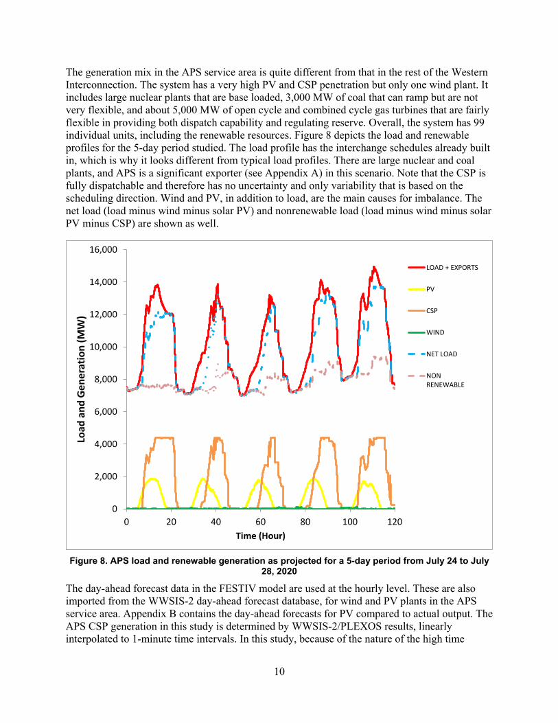
The generation mix in the APS service area is quite different from that in the rest of the Western Interconnection. The system has a very high PV and CSP penetration but only one wind plant. It includes large nuclear plants that are base loaded, 3,000 MW of coal that can ramp but are not very flexible, and about 5,000 MW of open cycle and combined cycle gas turbines that are fairly flexible in providing both dispatch capability and regulating reserve. Overall, the system has 99 individual units, including the renewable resources. Figure 8 depicts the load and renewable profiles for the 5-day period studied. The load profile has the interchange schedules already built in, which is why it looks different from typical load profiles. There are large nuclear and coal plants, and APS is a significant exporter (see Appendix A) in this scenario. Note that the CSP is fully dispatchable and therefore has no uncertainty and only variability that is based on the scheduling direction. Wind and PV, in addition to load, are the main causes for imbalance. The net load (load minus wind minus solar PV) and nonrenewable load (load minus wind minus solar PV minus CSP) are shown as well.

Figure 8. APS load and renewable generation as projected for a 5-day period from July 24 to July

28, 2020

The day-ahead forecast data in the FESTIV model are used at the hourly level. These are also imported from the WWSIS-2 day-ahead forecast database, for wind and PV plants in the APS service area. Appendix B contains the day-ahead forecasts for PV compared to actual output. The APS CSP generation in this study is determined by WWSIS-2/PLEXOS results, linearly interpolated to 1-minute time intervals. In this study, because of the nature of the high time

0

2,000

4,000

6,000

8,000

10,000

12,000

14,000

16,000

0 20 40 60 80 100 120

Load

and

Gen

erat

ion

(MW

)

Time (Hour)

LOAD + EXPORTS

PV

CSP

WIND

NET LOAD

NONRENEWABLE

11

resolution modeling, a number of assumptions are made that can affect the results in one direction or the other, as seen in Table 3. However, all of these results are made consistent in each of the case studies, so that the comparisons are the important part of this research. The model ignores the transmission constraints within the footprint, as optimal geographic distribution of wind and solar is outside the scope of this study. Conventional generators follow AGC schedules perfectly throughout time, which is not realistic. The FESTIV model also does not model frequency response. These assumptions could underestimate the imbalance results. However, the simulation model is a model, and therefore cannot simulate the behavior of human operators making decisions to improve upon the optimal scheduling models. The study is also taking a lot of fixed data from previous WWSIS2 production cost model runs, with no chance for those runs to assist in additional flexibility from case to case. These assumptions can make the reliability impacts look worse than they may be. Finally, there are a number of assumptions that can have either effect. These include benchmarking, the validity of data used, and the limited time period of the study. We therefore reemphasize the interpretation of the results in subsequent sections to be focused on comparison and understanding of changes rather than predictions of the actual impacts that will occur.

Table 3. Assumptions Made in Simulations

Assumptions that might make reliability impact results look better than reality

Assumptions that might make reliability impact results look worse than reality

Assumptions that can make reliability impacts look better or worse than reality

No transmission effects are considered.

There is no human intervention or human intelligence in scheduling the resources.

There is no benchmarking on practices and data to exactly match current APS performance.

Conventional generators are assumed to follow their schedules perfectly.

Interchange schedules are taken from 5-minute WWSIS2 production cost results, not hourly schedules, and are fixed in FESTIV. They cannot change based on the different sensitivities.

Data from TEPPC database may not exactly match reality and has not gone through a rigorous validation process.

Primary frequency response (governor response) is not considered, nor is the frequency component of the ACE equation.

Concentrating Solar plant schedules are from WWSIS2 production cost results and are fixed in FESTIV.

Five-day study might not be representative for wider time intervals.

12

The Impacts of Photovoltaic Variability and Uncertainty We performed some base analysis to gain an understanding of the amount of imbalance on the system without any advanced mitigation strategies. Two types of reserve were used in this case with existing requirement methods. Contingency reserve is held but not deployed until it is a last resort and regulating reserve is continuously deployed by the AGC submodel. DASCUC, RTSCUC, and RTSCED all use co-optimization of both reserve types with energy. Contingency reserve was required to meet 3% of the hourly load. This is similar to the current WECC contingency reserve rule [13]. The regulating reserve was held to meet 1% of the hourly load, both upward and downward regulation, which is similar to how many areas procure their regulating reserve. The AGC uses the regulating reserve to correct the ACE (i.e., bring it down to zero). The AGC uses a smoothed ACE with a proportional and integral term. In our case, the smoothed ACE is averaged over the past 3 minutes to eliminate noise. This typical procedure is used in today’s systems as described in [14] and [15]. The RTSCUC and RTSCED are run at hourly resolution in the base case (i.e., tRTC, IRTC and tRTD, IRTD = 60 minutes). Many of the balancing areas in the Western Interconnection operate in this way today. The RTSCUC can start and stop any units that have a start-up time less than or equal to 1 hour. The DASCUC operates at hourly resolution as well, scheduling for a day at a time (HDAC = 24 hours) and repeating once a day at noon (tDAC = 24 hours). The DASCUC can start or stop any unit. RTSCUC schedules for a horizon of three intervals (HRTC = 3 hours) and RTSCED schedules for one interval (HRTD = 1 hour). Load forecasts are assumed to be perfect for all submodels. Day-ahead forecasts for PV and wind are taken from the WWSIS-2 study [10].

For illustrative purposes, perfect hourly forecasts are used in both RTSCUC and RTSCED for a 1-day simulation to give an example of the ACE, illustrated in Figure 9, with the L10 limit shown for comparison. The total ACE is a result of the subhourly variability of the load, PV, and wind, because there is no uncertainty. Note that the system is still being scheduled at an hourly time resolution for the dispatch, so whenever the regulation is not able to keep up with the variability within the hour, significant imbalance can result. In practice, a system operator will take actions to correct large imbalances instead of waiting the full 60 minutes to correct the issue. Because this is not done here, the imbalance may be higher than in reality. This operator action is explored later in the sensitivity cases. Although the ACE has swings that reach up to 100 MW, the swings are short and therefore not as significant as persistent excessive ACE. Generally, the ACE stays close to zero.

13

Figure 9. ACE 1-day simulation. Perfect PV forecasts are used in the real-time simulation.

To get a better idea of the imbalance, Figure 10 shows the ACE averaged over rolling 10-minute periods for every 1-minute interval to filter out noise. The NERC CPS2 standard requires 90% of all 10-minute averaged ACE levels to be below the L10 limit for a month. For reference, the current L10 for APS is 48 MW, and it should be increased to account for the increased 2020 load in this study. Figure 10 illustrates two instances where the ACE is persistently greater than 50 MW. These instances happen to occur at evening load drop-off, where, along with the morning load pickup, ACE and frequency issues regularly occur today (see, for example, [16] and [17]). For the most part, however, the ACE is kept to within –20 and 20 MW.

14

Figure 10. ACE averaged over rolling 10-minute periods for 1-day simulation. Perfect forecasts are

used in the real-time simulation.

Figure 11 shows the generation by category for this 1-day perfect forecasting simulation. Selected groups of units are shown for their 1-minute generation for the 1-day period. The high frequency noise seen for the conventional generating units, show the resources being given signals by AGC to regulate the load, wind, and PV variability that occurs within the hour. The CSP is used to follow the load pickup and drop-off as well as the interchange scheduling changes.

-150

-100

-50

0

50

100

150

0 1 2 3 4 5 6 7 8 9 10 11 12 13 14 15 16 17 18 19 20 21 22 23

Rolli

ng 1

0-m

inut

e av

erag

e AC

E (M

W)

Time (Hour)

Current L10 bounds

15

Notes: Palo Verde, nuclear; Ocotil, steam; Cholla and Four Corners, coal; Sundance, gas turbine type generators

Figure 11. Generation for 1-day perfect forecast

For our analysis of the PV effects, we now compare two full 5-day simulations. Case 1 does not include any PV on the system (wind and CSP are kept). PV is added in Case 2 assuming perfect real-time PV forecasts (day-ahead forecasts still have uncertainty). Figure 12 shows the total generation and load plus their interchange for the study period for Case 2. Overall, the generation follows the load quite well. In some instances, the variability is excessive and cannot be compensated as closely. For example, during hours 40 and 41 (highlighted rectangle), some excessive variability is seen in the load. The perfect forecasts for those hours were based on the hourly averaged load, which did not capture the subhourly variation. Similar instances occurred with the PV variability that was significantly above or below the hourly average. Even with perfect certainty in the hourly forecast, excessive imbalance can be caused by the resolution of the scheduling interval. Some areas and studies have been proposing additional flexibility reserve (e.g., following reserve from Figure 2) that can be used to mitigate this variability [6].

0

500

1,000

1,500

2,000

2,500

3,000

3,500

4,000

4,500

5,000

0 1 2 3 4 5 6 7 8 9 10 11 12 13 14 15 16 17 18 19 20 21 22 23 24

Gene

ratio

n (M

W)

Time (Hour)

PVCSPWindFour CornersPalo VerdeChollaBlack MountainGila RiverOcotilSaguarAZSundanceRedHawkWest PhoenixYucca

16

Figure 12. Total generation and load for 5-day perfect forecast base case

We set the L10 level for CPS2 to 65 MW in this study to account for projected load growth in 2020. Case 1 results in 36 violations while the perfect hourly PV forecast case results in 29 violations of L10, leaving a CPS2 score of about 95.2% and 96.0%, respectively. Both scores meet the NERC criteria. Adding the perfectly forecasted PV reduced the amount of CPS2 violations, which is counterintuitive. There are instances where the load was increasing significantly within the hour during the morning load pickup. The PV was also ramping up which acted as additional regulating reserve meeting the ramp requirement and avoided some 10 minute intervals that initially had violated CPS2. While it reduced a few occasions of significant imbalance, the perfectly forecasted PV did increase the total imbalance from 2,690 MWh to 2,976 MWh of AACEE, or about 22.4 to 24.8 MW of ACE per hour. The PV also increased the σACE from 49.8 to 51.2 MW. As expected, the total production cost of electricity decreased from $15.040 million to $12.061 million with the zero-cost PV added, or from $12.21/MWh to $9.79/MWh of load.

The comparisons made when adding PV to the system with perfect hourly forecasts show the impact of minute-to-minute variability of PV on the system when scheduling at hourly time frames. Next, we study the real-time uncertainty impacts that occur from solar PV and wind by adding realistic forecast errors to the real-time scheduling models RTSCUC and RTSCED. The case study now uses a persistence forecast for wind power and a persistent cloudiness forecast for solar PV. This means that for wind, the actual output when the RTSCED or RTSCUC model started is the forecast for 1 hour ahead. For PV, this means that the current cloudiness will remain constant for the predicted output, but the typical rise and fall based on the sun during clear sky conditions are incorporated into the forecast. This is described in the following equation, taken from [18]. PF is the forecast, P is the output, PCS is the clear sky output, and SPI is the solar power index (P/PCS). Note that in the base case simulation, ∆t is 60 minutes plus the

17

simulated time it takes to run the model (e.g., IRTD + PRTD). In total, this results in 65 minutes for RTSCED and 75 minutes for RTSCUC.

𝑃𝐹(𝑡 + ∆𝑡) = 𝑃(𝑡) + 𝑆𝑃𝐼(𝑡) ∗ [𝑃𝐶𝑆(𝑡 + ∆𝑡) − 𝑃𝐶𝑆(𝑡)]

Table 4 shows the performance characteristics for PV and wind when using these forecast methods and the 60-minute RTSCED. The wind persistence forecast is not great because of the long, 60-minute look-ahead horizon. The PV forecast is more accurate (in terms of percentage of nameplate), but because of the higher installed PV capacity, the uncertainty in its forecast has a significant effect. The PV forecast is also slightly overforecasting on average.

Table 4. Forecast Performance for 5-Day Period Using Persistence (Wind) and Persistent Cloudiness (PV) for 60-Minute RTSCED 5-Day Period

Bias (MW / % of nameplate)

MAE (MW / % nameplate)

Standard Deviation (MW / % of nameplate)

PV 23.0 / 0.8 55.4 / 1.9 88.4 / 3.0

Wind –1.0 / –0.3 11.6 / 3.9 18.7 / 6.0 Note: MAE, mean absolute error The forecast uncertainty increases the imbalance. The simulation results show 55 CPS2 violations, resulting in a 92.4% score, which is closer to the 90% limit of CPS2 compliance, but still above. Overall, there is 3,530 MW of AACEE, resulting in about 29.4 MW of ACE per hour. The σACE results in 61.2 MW, a 20% increase than Case 2. Total production costs are $12.036 million, slightly lower than those from the perfect hourly forecast case.2 The system cost less because it did not spend extra when regulation reserve ran out. This mirrors the conclusion that although they may have great impacts on reliability, real-time forecast errors typically do not have significant impacts on production costs when everything else remains equal [1]. It is important to reiterate that the same load and VG output is realized in Case 2 and Case 3, and every remaining case, other than Case 1 which uses the same data except without PV. Table 5 compares these three cases. Appendix C gives the full ACE values for all case studies. Comparing Case 2 with Case 1 shows the variability impacts of the added solar PV. Comparing Case 3 with Case 2 shows the uncertainty impacts of PV and wind. For this period, and this system, the imbalance impacts of forecasting imperfectly are far greater than the effects of variability of the PV alone. With this base understanding of how variability and uncertainty of PV affect the system imbalance, we now focus on outlining different strategies to attempt to reduce the imbalance of these variability and uncertainty impacts, while also attempting to limit significant production cost increase.

2 In all cases, the total amount of ACE for the study period, must be paid back (if negative) or sold (if positive) at the average LMP, to ensure total costs are comparable between cases. This is similar to paying back inadvertent interchange.

18

Table 5. Comparison of Variability and Uncertainty Impacts

Case CPS2 Score AACEE (MWh)

σACE (MW) Production Costs

($million) Case 1: No PV 35 violations

95.2% 2,690 49.8 $15.040

Case 2: Perfect real-time forecast at 60-minute intervals (variability impacts)

29 violations 96.0%

2,976 51.2 $12.061

Case 3: Imperfect real-time forecast at 60-minute intervals (variability and real-time uncertainty impacts)

55 violations 92.4%

3,530 61.2 $12.036

19

Imbalance Reduction Strategies Operator Action In the first three case studies, dispatch and commitment in real time were performed at 60-minute intervals. Excessive ACE could occur within the dispatch interval, but would not be corrected until the next hour. In reality, when the system is not in balance, operators would intervene and direct resources to change their dispatch or commitment to correct the imbalance. This is similar to operators deploying contingency reserve during contingencies. To simulate operator action, we use the RPU option built within FESTIV. The commitment and dispatch will continue to run at tRTC = tRTD = 60 minute intervals; however, if excessive ACE occurs within the hour, the operator would run the RPU to correct the imbalance. For this, if the ACE exceeds the L10 (65 MW) in either direction, the operators would run the RPU to correct the imbalance immediately instead of waiting for the next automatic RTSCED or RTSCUC run. The RPU uses a single 10-minute interval in which commitment and dispatch decisions are made. Table 6 shows the results.

Table 6. Utilization of Operator Action Using RPU




95.2% 2,690 49.8 $15.040


29 violations 96.0%

2,976 51.2 $12.061


55 violations 92.4%

3,530 61.2 $12.036

Case 4: Imperfect real-time forecasts at 60-minute intervals with RPU

28 violations 96.1%

2808 45.1 $12.577

The operator action reduced the amount of CPS2 violations significantly, down to the level of perfect real-time forecast case (Case 2). The RPU run also reduced the AACEE to 2,808 MWh and σACE to 45.1 MW, with the σACE being lower than that of the perfect real-time forecast case (Case 2) and no PV case (Case 1). This highlights the fact that the use of operator action to reduce ACE off the nominal scheduling intervals will mitigate some of the variability impacts as well as the uncertainty impacts. Since the standard deviation and CPS2 violations were reduced below Case 1, but AACEE was not, this can suggest that there was a greater focus on reducing significant imbalances than reducing the overall amount of ACE. In other words, when the operator noticed the large imbalance he would correct it, but the operator would have ignored imbalances when ACE was occurring that was not leading to a reliability issue. The use of the operator action increased the total production costs by a fair amount. Case 2 and Case 3 were very close in total production costs, but the RPU case resulted in over a $500,000 (greater than 4%) increase, or about $0.50 per MWh. So, even though the use of operator action with the use of RPU to respond to the excessive imbalances allowed the system to greatly reduce the ACE impacts, doing so was costly. These off-nominal-time actions occurred very rarely when PV was not producing, and occurred on average about 30 times a day, or a little more than once an hour.

20

Improved Day-Ahead Forecasts The case studies so far have focused on the real-time uncertainty impacts of PV and wind. In the next case study, we fix the day-ahead forecasts to perfectly match the hourly average of PV and wind generation, but keep the real-time forecasts imperfect as in Case 3 and Case 4. Studies have shown that perfect day-ahead wind and PV forecasts reduce the production costs of the system by improving the efficiency of the unit commitment decision [19]. The impact of day-ahead PV forecasts on imbalance and ACE metrics, however, has not been studied sufficiently. Table 7 shows the day-ahead forecast performance and Table 8 shows the results for the perfect day-ahead forecast case.

Table 7. Day-Ahead Forecast Performance for 5-Day Period for DASCUC

Bias (MW / % of nameplate)

MAE (MW / % nameplate)

Standard Deviation (MW / % of nameplate)

PV 53.6 / 1.8 94.2 / 3.2 149.7 / 5.1

Wind 15.8 / 5.2 37.7 / 12.6 60.8 / 20.3

Table 8. Day-Ahead Uncertainty Impact Improvements


σACE (MW)

Production Costs ($million)

Case 1: No PV 35 violations 95.2%

2,690 49.8 $15.040


29 violations 96.0%

2,976 51.2 $12.061


55 violations 92.4%

3,530 61.2 $12.036

Case 5: Imperfect real-time forecast at 60-minute intervals with perfect DA forecasts

54 violations 92.5%

3,574 61.2 $11.938

The imbalance results are not changed significantly from Case 3, since the real-time forecasts are identical. The total production costs are reduced to $11.938 million, the lowest total cost yet, but at less than 1%, perhaps not as much as is normally the case for wind power day-ahead forecast improvements [19]. This likely results from the fact that day-ahead forecast errors for PV are not as significant as day-ahead forecast errors for wind. This can be seen with a comparison of Table 7 with Table 4. Although the day-ahead wind forecast error is significantly greater for the day-ahead forecasts compared to the real-time forecast error (MAE is increased by about 3 times), the day-ahead forecast error for PV is not as significant (MAE is increased by about 1.5 times). This could show that the improvements in real-time or short-term solar PV forecasts are more important than improvements to day-ahead solar PV forecasts.

Increased Dispatch Frequency Many studies and areas are showing the cost benefits of increasing the dispatch frequency to faster scheduling intervals, for example [20]. Few, however, have shown the reliability benefits for reducing imbalance. Faster dispatch frequency has the advantage of having the information at

21

a more granular scale, so that imbalance can be corrected more often through dispatch instead of limited AGC resources. This has the effect of reducing the subhourly variability impacts. It also has the advantage of improving real-time forecasts because the look-ahead interval is shortened, reducing the real-time uncertainty impacts. For this case study, we operate the RTSCED at tRTD = IRTD = 5 minutes, with the total forecast horizon being 10 minutes (i.e., IRTD + PRTD). Table 9 shows the RTSCED forecast errors, which are significantly reduced for both the persistent cloudiness PV forecast and for the persistence wind forecast. In addition, the forecast bias is now essentially eliminated.

Table 9. Forecast Performance for 5-Day Period Using Persistence (Wind) and Persistent Cloudiness (PV) for 60-Minute RTSCED 5-Day Period

Bias (MW/% of nameplate)

Mean Absolute Error (MW/% nameplate)

Standard Deviation (MW/% of nameplate)

PV (5 minutes) 0.3 / 0.0 20.3 / 0.7 34.6 / 1.1

PV (60 minutes) 23.0 / 0.8 55.4 / 1.9 88.4 / 3.0

Wind (5 minutes) 0.0 / 0.0 7.8 / 2.6 12.3 / 4.1

Wind (60 minutes) –1.0 / 0.3 11.6 / 3.9 18.7 / 6.0 Because the RTSCUC is kept constant at 60-minute resolution and update frequency, additional commitments of quick-start resources do not help in this case. The results are influenced only by improving the persistence wind forecast and persistent cloudiness PV forecasts, and by better dispatching of 5-minute variability. Table 10 shows the results.

Table 10. Impact of 5-Minute Dispatch




95.2% 2,690 49.8 $15.040


29 violations 96.0%

2,976 51.2 $12.061


55 violations 92.4%

3,530 61.2 $12.036

Case 6: Imperfect real-time forecasts at 5-minute intervals

24 violations 96.7%

2,305 46.2 $11.938

Using the 5-minute RTSCED operation has significantly improved the imbalance results. There are only 24 CPS2 violations throughout the 5-day simulation, resulting in a 96.7% score. The AACEE and σACE are also reduced to 2,305 MWh (19.2 MW of ACE per hour) and 46.2 MW, respectively. The three ACE metrics have been improved the greatest yet. In fact, all metrics fall to significantly below those seen in Case 1, the case without PV. The likely reason is that the load variability impacts in Case 1 were reduced by the 5-minute dispatch in addition to the reduction of the PV and wind variability and real-time uncertainty impacts. The production costs are also decreased, showing that reducing those impacts with the 5-minute dispatch does not have high costs.

22

Regulation Reserve Increase As discussed earlier, regulation reserve is the reserve the AGC uses to correct the minute-to-minute imbalance in between the dispatch intervals. In the following example, we increase the regulation reserve for the 5-minute case (Case 6) to see how the increased regulation reserve affects the imbalance. For further information on how studies have been proposing increases in regulation reserve, see [4]. In this case study, we apply the methodology used in the WWSIS-2 study, detailed in [18]. It accounts for uncertainty present in the wind and PV by assessing the 95th percentile of annual 10-minute-ahead forecast errors. The 10-minute time frame was again based on the 5-minute dispatch and process time (as in the previous case, IRTD + PRTD = 10 minutes). The regulation requirement was then determined based on the expected error with explanatory variables of the solar power index and clear sky ramp. In other words, the extent of cloudiness and the anticipated typical solar ramp are used to predict the regulation reserve requirement each hour. The wind component was based on the wind output alone. These components were added geometrically with each other and 1% of the load from the previous requirement to arrive at the new hourly regulation reserve requirement. Figure 13 compares the two reserve methods in both upward and downward directions.

Figure 13. Regulation reserve requirements for Cases 1–6 (1% load) and Case 7 (WWSIS-2 [18])

-250

-200

-150

-100

-50

0

50

100

150

200

250

0 20 40 60 80 100 120

Regu

latio

n Re

quire

men

t (M

W)

1% Regulation Up 1% Regulation Down WWSIS-2 Regulation Up WWSIS-2 Regulation Down

23

Now Case 7 is run with identical properties to Case 6, but for the increased regulation reserve requirements. Table 11 gives the results.

Table 11. Impact of Increased Regulation Requirements




95.2% 2,690 49.8 $15.040


29 violations 96.0%

2,976 51.2 $12.061


55 violations 92.4%

3,530 61.2 $12.036


24 violations 96.7%

2,305 46.2 $11.938

Case 7: Imperfect real-time forecasts at 5-minute intervals, with increased WWSIS2 regulation reserves

22 violations 96.9%

2055 41.7 $12.005M

With the increased regulation reserve requirements, the CPS2 violations are reduced slightly from 24 to 22 violations, resulting in a 96.9% CPS2 score. The AACEE and σACE are also reduced to the lowest levels yet at 2055 MWh (17 MW of ACE per hour) and 41.7 MW, respectively. The increased regulation reserve requirements raise the production costs by $67,000. This cost increase is not trivial (0.6%), but perhaps justified if a better CPS2 score is needed. The intelligent manner of only increasing the requirements during instances when the PV and wind might have higher variability and uncertainty, has likely led to the minimal increase in production costs. Then again, if the CPS2 score is already well above the NERC criteria, perhaps the increased requirements might not be necessary.

24

Conclusion All case study results are shown in Table 12. The first three cases show the base case impacts of PV variability and uncertainty, and the next four cases illustrate the effects of the mitigation strategies that can be used to reduce these impacts. Figure 14 shows the CPS2 scores along with production costs for all PV cases. The goal is to have high CPS2 scores and low production costs. For comparison of full 5-day ACE results for all cases, see Appendix C.

Table 12. Case Comparisons

Case VG Forecast Mitigation Strategy

CPS2 Score AACEE (MWh)

σACE (MW)

Production Costs

($million) Case 1 N/A

(No PV) None (60-minute schedule)

35 violations 95.2%

2,690 49.8 $15.040

Case 2 Perfect real-time Imperfect day-ahead

None (60-minute schedule)

29 violations 96.0%

2,976 51.2 $12.061

Case 3 Imperfect real-time and day-ahead

None (60-minute schedule)

55 violations 92.4%

3,530 61.2 $12.036


RPU (operator action)

28 violations 96.1%

2808 45.1 $12.577

Case 5 Imperfect real-time Perfect day-ahead

Perfect day-ahead forecast

54 violations 92.5%

3,574 61.2 $11.938


5-minute schedule 24 violations 96.7%

2,305 46.2 $11.938


5-minute schedule, increased regulation reserves

22 violations 96.9%

2,055 41.7 $12.005

25

Figure 14. CPS2 scores and production costs for all PV cases

This study, which compares imbalance results with those of production costs, analyzed the impacts of solar photovoltaic, along with impacts of other sources like load and wind, at multiple operational timescales. Although many of the previous studies focused primarily on production costs, this study aimed to show how imbalance and active power control standards were changed with variability and uncertainty of these sources along with production costs. We used FESTIV to quantify the variability and uncertainty impacts of solar PV, and then to determine how numerous mitigation strategies perform in trying to reduce those impacts. The real-time uncertainty impacts certainly had a greater impact on imbalance than did the PV variability. We even showed that perfectly predicted PV, when spread over large geographic areas as they were in this study, could reduce imbalance impacts when the PV was providing additional ramping capability coinciding with load variability. We also determined that the real-time uncertainty of PV had little impact on production costs. Day-ahead PV forecasts, however, when improved, had little impact on variability and uncertainty imbalance impact reduction. They were able to reduce production costs, but not as significantly as has been seen with wind forecasts. Operator action seemed to improve the imbalance impacts with a focus on reducing the larger noticeable imbalances. However, it involved significant incremental production costs. Moving from a 60-minute dispatch to a 5-minute dispatch appeared to be a good option. This greatly reduced the variability and uncertainty impacts, even from the case without PV, and did not increase production costs. Increasing the regulation reserve requirements had a positive impact on reducing the imbalance impacts even further. The question would be whether or not the

26

improvements in reducing imbalance are worth the marginal increase in production cost, if the reliability criteria have already been exceeded.

This study is a snapshot into analyzing imbalance impacts with costs. Our work demonstrates how multiple metrics can be used to measure the reliability impacts and the production cost impacts together. Each of these metrics may have different meaning and different value to different balancing areas, and it is important to create strategies that fit the goals of that area. Full reliability analysis would require significantly more analysis on other aspects such as frequency response, adequacy, voltage stability, and transient stability. This study considers only the active power imbalance on a particular balancing area, ignoring the rest of the interconnection (other than the modeling of the interchange schedules). Further studies can evaluate more scheduling strategies, including more optimal operating reserve requirement methodologies. As the industry continues to evolve and integrates higher quantities of renewable resources on the power system, these methods could be adopted if they prove superior to current methods.

27

References [1] Ela, E.; O’Malley, M. “Studying the Variability and Uncertainty of Variable Generation

at Multiple Timescales.” IEEE Transactions on Power Systems (27:3), pp. 1324-1333, August 2012.

[2] Mills, A. et al. Understanding Variability and Uncertainty of Photovoltaics for Integration with the Electric Power System. Technical Report LBNL-2855E. Berkeley, CA: Lawrence Berkeley National Laboratory, 2009.

[3] Western Wind and Solar Integration Study. NREL/SR-550-47434. Work performed by GE Energy, Schenectady, NY. Golden, CO: National Renewable Energy Laboratory, 2010.

[4] Ela, E.; Milligan, M.; Kirby, B. Operating Reserves and Variable Generation. NREL/TP 5500-51978. Golden, CO: National Renewable Energy Laboratory, August 2011.

[5] North American Electric Reliability Corporation. “Reliability Standards for the Bulk Electric Systems of North America,” Available: www.nerc.com, June 2012.

[6] Navid, N.; Rosenwald, G.; Chatterjee, D. Ramp Capability for Load Following in the MISO Markets. Version 1.0. Carmel, IN: MISO, July 2011. Accessed March 18, 2013: https://www.midwestiso.org/Library/Repository/Communication%20Material/Key%20Presentations%20and%20Whitepapers/Ramp%20Capability%20for%20Load%20Following%20in%20MISO%20Markets%20White%20Paper.pdf.

[7] Ela, E.; Milligan, M.; O’Malley, M. “A Flexible Power System Operations Simulation Model for Assessing Wind Integration.” 2011 IEEE Power & Energy Society General Meeting, “The Electrification of Transportation & The Grid of the Future. July 24–28, 2011, Detroit, Michigan.”.

[8] GAMS Development Corporation. GAMS: The Solver Manuals. Version 23.9. Washington, DC: GAMS, 2011.

[9] Ferris, M. MATLAB and GAMS: Interfacing Optimization and Visualization Software. Mathematical Programming Technical Report 98-10. Madison, WI: University of Wisconsin Computer Sciences Department, 2005.

[10] D. Lew et al., The Western Wind and Solar Integration Study Phase 2. Forthcoming. [11] WECC TEPPC. 2009 Study Program Results Report, YEAR. Accessed Sept. 2012:

www.wecc.biz/committees/BOD/TEPPC/Shared Documents/TEPPC Annual Reports/. 2009

[12] National Renewable Energy Laboratory, Wind Integration Datasets. http://www.nrel.gov/wind/integrationdatasets.

[13] WECC. Western Electricity Coordinating Council Minimum Operating Reliability Criteria, April 2005. Accessed Sept., 2012: http://www.wecc.biz/Standards/Development/WECC%200099/Shared%20Documents/WECC%20Reliability%20Criteria%20MORC%202005.pdf.

[14] Jaleeli, N.; VanSlyck, L.S.; Ewart, D.N.; Fink, L.H.; Hoffmann, A.G. “Understanding Automatic Generation Control.” IEEE Transactions on Power Systems (7:3), August 1992; pp. 1106–1122.

[15] Report: ENTSO-E, UCTE Operational Handbook Policy 1, Load-Frequency Control and Performance, March 2009.

[16] NERC. 22:00 Frequency Excursions (Final Report). NERC Frequency Excursion Task Force, August 28, 2002.

28

[17] Weissbach, T.; Welfonder, E. “High Frequency Deviations within the European Power System: Origins and Proposals for Improvement.” Proceedings of the Power Systems Conference and Exposition, March 15–18, 2009, Seattle, Washington.

[18] Ibanez, E.; Brinkman, G.; Hummon, M.; Lew, D. “A Solar Reserve Methodology for Renewable Energy Integration Studies Based on Sub-Hourly Variability Analysis” 2nd International Workshop on Integration of Solar Power in Power Systems, November 12–13. 2012, Lisbon, Portugal.

[19] Lew, D.; Milligan, M.; Jordan, G.; Piwko, R. “The Value of Wind Power Forecasting.” Proceedings of 91st American Meteorological Society Annual Meeting, January 23–27, 2011, Washington, D.C.

[20] Milligan, M.; Kirby, B.; Beuning, S. “Combining Balancing Areas’ Variability: Impacts on Wind Integration in the Western Interconnection.” AWEA WindPower 2010, Golden, CO: National Renewable Energy Laboratory, July 2010.

29

Appendix A: Load and Interchange

0

2,000

4,000

6,000

8,000

10,000

12,000

14,000

16,000M

W

APS Load+Export APS Load Exports

30

Appendix B: Day-Ahead Photovoltaic Forecast and Actual Photovoltaic Generation

31

Appendix C: Area Control Error Charts (Case 1–Case 7 in Order)

Case 1: No PV

32


Case 3: Imperfect real-time forecast at 60-minute intervals (variability and real-time

uncertainty impacts)

33

Case 4: Imperfect real-time forecasts at 60-minute intervals with RPU

Case 5: Imperfect real-time forecast at 60-minute intervals with perfect DA forecasts

34


Case 7: Imperfect real-time forecasts at 5-minute intervals, with increased WWSIS2

regulation reserves