impacts of climate change on water resources of nepal the
TRANSCRIPT

Impacts of Climate Change on Water Resources of Nepal
The Physical and Socioeconomic Dimensions
Dissertation Zur Erlangung des Grades:
Doktor der Wirtschaftswissenschaften (Dr. rer. Pol.) an der Universität Flensburg
von
Narayan Prasad Chaulagain, M. Sc. Nepal
Flensburg, 2006

ii
Gutachter : 1. Prof. Dr. Olav Hohmeyer (Betreuer)
Universität Flensburg Internationales Institut für Management Energie- und Umweltmanagement
2. Prof. Dr. Stephan Panther Universität Flensburg Internationales Institut für Management
3. PD Dr. Sc. Alfred Becker Potsdam Institute for Climate Impact Research

iii
Contents
List of tables vi
List of figures vii
Acronyms and abbreviations ix
Acknowledgement xi
Abstract xii
1 Problem statement and objectives of the study 1
1.1 Background of the study and problem statement 1
1.2 Objectives 5
1.3 Organisation of the report 6
2 State-of-the-art review and development of hypotheses 7
2.0 General 7
2.1 Global climate change 7
2.1.1 Global temperature change 8
2.1.2 Change in precipitation and atmospheric moisture 10
2.2 Climate change in the Himalayan region and Nepal 11
2.2.1 Climate change in the Himalayas 11
2.2.2 Climate Change in Nepal 13
2.2.2.1 Change in temperature 14
2.2.2.2 Change in precipitation 14
2.3 Physical impacts of climate change 15
2.3.1 Impacts on water resources and hydrology- a global perspective 15
2.3.2 Impacts of climate change on water resources – the Himalayan perspective 17
2.3.2.1 Snow and glacier 17
2.3.2.2 River discharge 19
2.4 The socioeconomic impacts 20
2.4.1 Effects on the water withdrawals 21
2.4.2 Agriculture and food security 21
2.4.3 Effects on the hydropower potential 23
2.4.4 Effects on extreme events 24
2.4.4.1 Changes in flood and drought frequency 24

iv
2.4.4.2 Glacier lake outburst floods 25
2.5 Projected future climate 27
2.5.1 Future global climate 27
2.5.2 Climate change scenarios for Nepal 27
2.6 Open questions 28
2.7 Development of hypotheses 29
3 Research methodology 30
3.1 Study design and context 30
3.2 Source of data 30
3.3 Detecting the climate change 31
3.3.1 Testing for significance 32
3.4 Estimating the physical impacts of climate change 34
3.4.1 Impacts of climate change on river runoff: the Water Balance Model - WatBal 34
3.4.2 Impacts on glacier mass balance in the Nepal Himalayas 36
3.4.2.1 Empirical glacier mass balance model 37
3.4.2.2 Application of the empirical glacier mass balance model 38
3.4.2.3 Sensitivity of the glaciers in the Nepal Himalayas to temperature rise 39
3.5 Estimating the socioeconomic impacts of climate change 40
3.5.1 Impacts on the total water availability in Nepal 41
3.5.2 Impacts on the hydropower potential 41
3.5.3 Impacts on the water balance situation 42
3.5.3.1 The FAO Penman-Monteith method 43
3.5.4 Climate change impacts on agricultural production, poverty and food security 44
3.5.5 Impacts on extreme weather events 44
3.6 Limitations of the study 45
4 Empirical findings on climate change in Nepal 46
4.0 General 46
4.1 Temperature change 46
4.1.1 Empirical findings on temperature change 46
4.1.2 Discussion of empirical findings on temperature change 48
4.2 Precipitation change 51
4.2.1 Empirical findings on change in precipitation amount 51

v
4.2.2 Empirical findings on change in number of rainy days 52
4.2.3 Discussion of empirical findings on precipitation change 54
4.3 Conclusion 55
4.3.1 Summary of findings 55
4.3.2 Open questions 56
5 Empirical findings on the physical impacts 57
5.0 General 57
5.1 Impacts on evapotranspiration and moisture balance 57
5.1.1 Empirical evidence on impacts on evapotranspiration and moisture balance 57
5.1.2 Discussion about the impacts on evapotranspiration and moisture balance 60
5.2 Impacts on the river flows 60
5.2.1 Runoff modelling of the Bagmati River at Chovar 62
5.2.2 Runoff modelling of the Langtang Khola at Langtang 64
5.2.3 Synthesis of the runoff modelling of the Bagmati River and the Langtang Khola 65
5.2.4 Discussion of the empirical evidence on the impacts on the river flows 69
5.3 Impacts of a temperature rise on snow and glacier systems 70
5.3.1 General findings 70
5.3.2 Sensitivity analysis of glacier mass balance to temperature rise 72
5.3.3 Discussion about the impacts of climate change on snow and glaciers 80
5.4 Conclusion 83
5.4.1 Summary of findings 83
5.4.2 Open questions 84
6 Empirical findings on the socio-economic impacts of climate change 85
6.0 General 85
6.1 Impacts on the water balance, agriculture and food security 85
6.1.1 Impacts on the irrigation water requirement 85
6.1.2 Impacts on the water balance situation 87
6.1.3 Impacts on the agricultural production, food security and poverty 90
6.1.4 Discussion of the impacts of climate change on water balance, Agriculture
and food security 97
6.2 Impacts on the hydropower potential 99
6.2.1 Empirical findings of the impacts on the hydropower potential 99

vi
6.2.2 Discussion of impacts on the hydropower potential 103
6.3 Impacts on the extreme events 104
6.3.1 Impacts on the glacier lake outburst floods 104
6.3.2 Impacts on droughts, floods and landslides 108
6.3.2.1 Snow-covered area and the extreme floods 108
6.3.2.3 Droughts, floods and landslides caused by the changing precipitation pattern 111
6.3.3 Discussion of the impacts of climate change on the extreme events 114
6.4 Conclusion 116
6.4.1 Summary of the findings 116
6.4.2 Open questions 116
7 Conclusions and recommendations 118
7.0 General 118
7.1 Conclusions 118
7.2 Recommendations 119
7.3 Propositions for future research 121
Bibliography 123
Annex

vii
List of Tables Table 2.1 GCM estimates of temperature and precipitation changes for Nepal 28
Table 3.1 Descriptions of reference meteorological stations 31
Table 4.1 Annual and seasonal mean temperature trends of reference stations 47
Table 4.2 Minimum, maximum and mean annual temperature trends 48
Table 4.3 Annual temperature trends of reference stations for 1988-2000 48
Table 4.4 Analysis of trends in annual precipitation records 51
Table 4.5 Fluctuations of number of rainy days at reference stations 52
Table 4.6 Trends in number of rainy days as per daily precipitation 53
Table 4.7 Analysis of precipitation at Rampur, Kathmandu and Daman 54
Table 5.1 Sensitivity analysis of atmospheric moisture to a temperature rise 58
Table 5.2 Sensitivity of soil moisture storage with a temperature rise at Kathmandu Airport 59
Table 5.3 Precipitation and runoff of the Langtang Khola and the Bagmati River 61
Table 5.4 Sensitivity of the river runoff to climate change at the Chovar station 63
Table 5.5 Sensitivity of the Langtang Khola runoff to climate change 65
Table 5.6 Sensitivity of monthly runoff to temperature and precipitation changes 67
Table 5.7 Summary of sensitivity analysis of glaciers at Langtang 74
Table 5.8 Glacier mass balance rates with different temperature change scenarios 76
Table 5.9 Sensitivity of glacier ice-reserve to a temperature rise in Nepal 77
Table 6.1 Sensitivity of potential evapotranspiration to a temperature rise 86
Table 6.2 Sensitivity of the irrigation water requirement to a warming 87
Table 6.3 Water supply and demand situation at Chovar 89
Table 6.4 Poverty analysis and measurement in Nepal 91
Table 6.5 Sensitivity of calorie supply to a warming for average population 95
Table 6.6 Sensitivity of calorie supply to a warming for different income groups 96
Table 6.7 All-Nepal average monthly and annual hydrograph 100
Table 6.8 Sensitivity of hydropower potential in Nepal with temperature rise 101

viii
Table 6.9 Sensitivity of hydroenergy potential in Nepal with temperature rise 102
Table 6.10 Sensitivity of melt- and rainwater to temperature change in Nepal 105
Table 6.11 Snow-covered areas and the ratio of maximum to minimum instantaneous
flows in some selected hydrological stations 108
Table 6.12 Sensitivity of snowfall to temperature increases in the Nepal Himalayas 112
Table 6.13 Sensitivity of rainfall to temperature increases in the Nepal Himalayas 113
List of Figures
Figure 2.1 Variations of the earth’s surface temperature 9
Figure 2.2 Annual temperature trends for 1976-2000 9
Figure 2.3 Annual precipitation trends for 1900-2000 10
Figure 2.4 Temperature trend as a function of elevation on the Tibetan Plateau 12
Figure 3.1 Conceptualization of water balance for the WatBal model 35
Figure 4.1 Mean temperature anomalies (1971-2000) 46
Figure 4.2 Fluctuation of standardised precipitation (1971-2000) 52
Figure 5.1 Mean monthly moisture balance at Kathmandu Airport 58
Figure 5.2 Comparative mean monthly hydrographs 61
Figure 5.3a Modelling the Bagmati River Runoff at Chovar (1976-1980) 63
Figure 5.3b Modelling the Langtang Runoff at Langtang (1993-1998) 64
Figure 5.4 Sensitivity of the runoff to temperature at Chovar 66
Figure 5.5 Sensitivity of runoff to precipitation at Chovar 67
Figure 5.6 Comparative sensitivity of river runoff (T+2, P-10 scenario) 68
Figure 5.7 Basin areas at Langtang 70
Figure 5.8 Average glacier mass balance with altitudes 71
Figure 5.9 Monthly glacier mass balances at Langtang 72
Figure 5.10 Sensitivity of glacier mass balance in altitudes 73
Figure 5.11 Sensitivity of glacier-ice reserve to a warming 76
Figure 5.12 Sensitivity of glacier surface area to a warming 78

ix
Figure 5.13 Distribution of glaciers with areas in Nepal 78
Figure 5.14 Sensitivity of glaciers to a warming in Nepal 79
Figure 5.15 Sensitivity of glacier-melt water to a warming 79
Figure 5.16 Sensitivity of total water availability to a warming in Nepal 80
Figure 6.1 Water balance at Chovar 88
Figure 6.2 Sensitivity of annual water balance situation at Chovar 89
Figure 6.3 Change in water balance at Chovar 90
Figure 6.4 Consumption patterns in Nepal 92
Figure 6.5 Sensitivity of hydropower potential to warming 101
Figure 6.6 Sensitivity of liquid water to a warming 105
Figure 6.7 Tsho Rolpa Glacier Lake and its development 107
Figure 6.8 Snow-covered area and extreme floods in Nepal 109
Figure 6.9 Hypothetical changes in peak discharges of the Bagmati River at Chovar 110

x
Acronyms and Abbreviations AD of the Christian era (from the Latin anno domini)
AET actual evapotranspiration
BP before present
CBS Central Bureau of Statistics, Nepal
CO2 carbon dioxide
DHMN Department of Hydrology and Meteorology, Nepal
DIO Department of Irrigation, Nepal
e.g. for example (from the Latin exempli gratia)
ELA equilibrium line altitude
et al. and others (from the Latin et alii)
etc. and so forth (from the Latin et cetera)
FAO Food and Agriculture Organization
GCM general circulation model
GDP gross domestic product
GLOF Glacier Lake Outburst Flood
GW gigawatt
i.e. that is (from the Latin id est)
ibid in the same book as previously mentioned (from the Latin ibidem)
ICIMOD International Centre for Integrated Mountain Development
IIASA International Institute for Applied Systems Analysis
IPCC Intergovernmental Panel on Climate Change
ISRSC Informal Sector Research and Study Center
km kilometre
km2 square kilometre
km3 cubic kilometre
kPa kilo Pascal
kPa ºC-1 kilo Pascal per degree centigrade
lpcd litre per capita per day
LRMP land resources mapping project
m metre
m w.e. metre of water equivalent
m2 square metre

xi
m2/yr square metre per year
m3 cubic metre
masl metre above sea level
MJ mega joule
mld million litres per day
mm millimetre
mm day-1 millimetre per day
MOF Ministry of Finance
MOPE Ministry of Population and Environment
ms-1 metre per second
MW megawatt
NDIN National Development Institute Nepal
NEA Nepal Electricity Authority
ºC degree centigrade
P precipitation
PET potential evapotranspiration
s second
T temperature
UK United Kingdom
UNDP United Nations Development Programme
UNEP United Nations Environment Programme
US United States
WECS Water and Energy Commission Secretariat
WGMS world glacier monitoring services
WMO World Meteorological Organization
yr year

xii
Acknowledgement
I would like to express my sincere gratitude to Prof. Dr. Olav Hohmeyer, director of
International Institute of Management, Energy and Environment Management for supervising
this dissertation as well as providing all kinds of support needed during my study in Germany.
Without his guidance, support and encouragement; this study could not have been realised.
Similarly, I am very grateful to Prof. Dr. Stephan Panther, International Institute of Management
for being the second supervisor of this dissertation. Likewise, I am greatly thankful to PD Dr. Sc.
Alfred Becker, Potsdam Institute for Climate Impact Research for being the external reviewer of
this dissertation as well as providing me other support and encouragement during the study.
I am also extremely thankful to the University of Flensburg, which provided me not only the
place to carry out this research, but also the financial support for my study in Germany. Without
this, it would not have been possible to complete this study. My heartfelt thank goes to Prof. Dr.
Hans Grothaus and Mrs. Ursula Grothaus for their support and encouragements. Similarly, kind
supports received during my study in Flensburg from Ms. Maike Borrmann, Ms. Ute Boesche-
Seefeldt, Ms. Janice Massey, Ms. Pam Lorenzen, Ms. Ingrid Nestle and Prof. Dr. Ursula Kneer
are also greatly appreciated.
Likewise, special gratitude goes to the Department of Hydrology and Meteorology of Nepal,
which kindly provided me hydrological and meteorological records for this research. Special
thanks go to Dr. M. L. Shrestha, Dr. K.P. Sharma, Dr. A. B. Shrestha, Dr. B. Rana, Dr. J. Bhusal,
Dr. D.K. Gautam, Mr. O. R. Bajracharya, Mr. S. Baidya, Mr. K. P. Budhathoki and Mr. N. R.
Adhikari. Similarly, Ms. Mandira Shrestha and Mr. P. K. Mool at the ICIMOD, Mr. Ajay Dixit
at the Nepal Water Conservation Foundation, Mr. Bikash Pandey at the Winrock International
Nepal, Mr. Tek B. Gurung at the UNDP Nepal, Dr. C.B. Gurung at the WWF Nepal, Prof. S. R.
Chalise, Dr. N. R. Khanal and Prof. Dr. K.L. Shrestha have also provided various kinds of
supports during this research. Their kind supports are greatly appreciated.
My heartfelt thanks and love to my wife Renuka for her continuous support and love, especially
when our daughter Akriti was born. Likewise, I am greatly thankful to my parents, son Abiral
and all my relatives for their love, encouragements and support.

xiii
Abstract The analysis of the long-term hydrological, meteorological and glaciological data from the Nepal
Himalayas has revealed that the climate in the Nepal Himalayas is changing faster than the
global average. Moreover, the changes in the high-altitudes have been found more pronounced
than in the low-altitudes. For example, annual temperatures at the Rampur station at an altitude
of 286 m were increasing at a rate of 0.04°C yr-1 while those at Kathmandu (1136 m), Daman
(2314 m) and Langtang (3920 m) were increasing by 0.05, 0.07 and 0.27 ºC yr-1 respectively.
Though no definite trends could be found in the annual precipitation records, clear decreasing
trends could be seen in the annual number of rainy days during the study period of 1971-2000.
The physical and socio-economic impacts of climate change with reference to water resources
were also assessed. Sensitivity analyses of river runoff, total water availability, glacier extent and
evapotranspiration to a temperature rise were also carried out. The analysis has revealed that the
glaciers in the Nepal Himalayas are shrinking rapidly and that there will be no glaciers left by
2180, if the current glacier melting rate continues. Most of the small glaciers will disappear
within 3-4 decades. There will be only 11% of the present glacier-ice reserve in the Nepal
Himalayas left by 2100, even if the present temperatures do not rise. Previous research and
present findings have shown a clear warming trend in the Nepal Himalayas, which will cause an
accelerated glacier melt. The accelerated glacier melt will increase the water availability at the
beginning but ultimately will reduce it after the glaciers disappear. For example, at a warming
rate of 0.06°C yr-1, Nepal’s total water availability may increase up to 178.4 km3yr-1 in 2030
from the present 176.1 km3yr-1 and then will drop down to 128.4 km3yr-1 in 2100. Warming
would increase the water requirement on the one hand and decrease the water supply on the
other. This will widen the gap between water supply and demand. Changing climate may further
exacerbate the water stress, which is already evident in Nepal due to the monsoon-dominated
climate. Almost every year in Nepal, there is a usual problem floods and landslides during the
rainy seasons because of too much water, whereas there is a common problem of droughts during
the dry seasons because of too little water. Climate change would further increase this seasonal
imbalance of water in Nepal.
Similarly, there will be substantial socioeconomic implications of reduced water availability. The
hydropower potential and agricultural production of Nepal would be seriously affected. A
reduction in agricultural production would have significant impact on the food security and

xiv
livelihoods of the subsistence farmers, who make up the majority of the Nepal’s population.
Nepal’s current income and food distribution is very uneven. For example, the poorest 20% of
the population of Nepal currently consume 6.2% of the total available food, while the richest
20% consume 53.3% of the total food. Currently, per capita daily calorie consumption of the
poorest 20% of the population is less than 40% of the minimum calorie requirement for carrying
out normal physical activities. Any further reduction in agricultural production may have
substantial negative impacts on the food security for these poorest people.

1
Chapter I: Problem Statement and Objectives of the Study
1.1 Background of the Study and Problem Statement Increasing numbers of scientific communities observing the global climate show a collective
picture of a changing climate and a warming world. The global average surface temperature
has increased by about 0.6ºC during the twentieth century (IPCC, 2001a, p 152). Many
analyses show that the temperature increase in the twentieth century has been greater than in
any other century during the past 1000 years (ibid). The 1990s was the warmest decade of the
millennium and 1998 was the warmest year on record (IPCC, 2001a, p.173). Natural and
human systems are expected to be exposed to direct effects of climatic variations such as
changes in temperature and precipitation variability, as well as frequency and magnitude of
extreme weather events. Similarly, there are indirect effects of climate change such as sea-
level rise, soil moisture changes, changes in land and water conditions, changes in the
frequency of fire and changes in the distribution of vector-borne diseases (ibid, p.245).
The hydrologic system, which consists of the circulation of water from oceans to air and back
to the oceans, is an integral part of the global climate system (Critchfield, 2002, p.249).
Therefore, any changes in the climate system cause not only changes in the hydrologic
system but also further modification of the climate itself due to these new changes in the
hydrologic system. Glaciers are very sensitive to climate changes; therefore, they can be
considered as good indicators of past climate changes (Nesje and Dahl, 2000, p.7).
Widespread retreat of the world’s glaciers was observed during the 20th century. The snow
covered area of the world has decreased by 10% since the 1960s (IPCC, 2001a, p.46). The
global mean sea level has increased at a rate of 1 to 2 mm/year during the 20th century due to
thermal expansion of sea water and the melting of glaciers and ice sheets (ibid). For example,
a local warming of 3ºC, if sustained for thousands of years, would lead to a virtually
complete melting of the Greenland ice sheet with a resulting sea-level rise of about 7 m
(IPCC, 2001a, p.84). Such a projected sea-level rise may threaten the existence of coastal
zones and their ecosystems.
Decreasing snow cover and the melting of glaciers as a result of warming provide positive
feedback to warming due to decreased surface albedo and increased absorption of solar
energy (Meehl, 1994, p.1033). The estimated quantity of the earth’s total water is about 1.4 x

2
109 km3, but only about 2.5% is fresh water. About 97% of the world’s water is contained in
the oceans. It is salty and not suitable for direct consumption (Singh and Singh, 2001, p.5).
Out of the available fresh water, about 77% (30x106 km3) is frozen in the polar ice caps and
in the glaciers of the world and the remainder is contained in the lakes, reservoirs, rivers,
atmosphere and in the aquifers under the ground (ibid, p.9). Therefore, the melting of ice-
sheets and glaciers due to warming is a threat to the limited freshwater reserves of the earth.
Climate change will result in more intense precipitation events causing increased flood,
landslide, avalanche and mudslide damages that will cause increased risks to human lives and
properties (IPCC, 2001a, p.226). Besides, intensified droughts are expected due to climate
change that may result in decreased agricultural productivity (ibid). Likewise, warmer
temperatures increase the water-holding capacity of the air and thus increase the potential
evapotranspiration, reduce soil moisture and decrease ground water reserves (IPCC, 2001b,
p.199), which ultimately affects the river flows and water availability.
The sensitivity of a hydrologic system to climate change is a function of several physical
features and societal characteristics. Some of the physical features most sensitive to climate
change are agriculture and livestock, regions with seasonal precipitation or snowmelt and
topography and land-use patterns that promote soil erosion and flash floods (IPCC, 2001b,
p.212). Similarly, the societal characteristics most susceptible to climate change are poverty
and low income levels, lack of water control structures, lack of human capital skills for
system planning and management, lack of empowered institutions, high population densities,
increasing demand for water because of rapid population growth and lack of formal links
among the various parties involved in water management (ibid, p.213).
Studies show that developing countries are more vulnerable to climate change and are
expected to suffer more from the adverse climatic impacts than the developed countries
(IPCC, 2001a, p. 287). In a humid climate like that of Nepal, there will be changes in the
spatial and temporal distribution of temperature and precipitation due to climate change,
which in turn will increase both the intensity and frequency of extreme events like droughts
and floods (Mahtab, 1992, p.37). Increases in temperature result in a reduced growing season
and a decline in productivity, particularly in South Asia (Pachauri, 1992, p.82). A warming
climate would increase water demand on the one hand and would decrease river flows on the
other. Reduced river flows will affect the hydro power generation, inland water transport and

3
aquatic ecosystem. Similarly, reduced water availability may create conflicts between water
users within and among nations (ibid, p.85).
Nepal is rich in water resources. There are more than 6000 rivers flowing from the
Himalayan Mountains to the hills and plains. Most of these rivers are glacier-fed and provide
sustained flows during dry seasons to fulfil the water requirements of hydropower plants,
irrigation canals and water supply schemes downstream. The hydrology of these rivers is
largely dependent on the climatic conditions of the region, which in turn is a part of global
climate. Accelerated melting of glaciers during the last half century has caused creation of
many new glacier lakes and expansion of existing ones (Mool et al., 2001a, p.121). There
have been more than 13 reported cases of glacier lake outburst flood events in the Nepal
Himalayas since 1964 causing substantial damage to people’s lives, livestock, land,
environment and infrastructure (Rana et al., 2000, p.563). Accelerated retreat of glaciers with
increased intensity of monsoon precipitation observed during recent years has most probably
contributed to increased frequency of such floods (Agrawala et al., 2003, p.28).
Nepal has about 83 GW of hydropower potential, but only about 1% of that has been
developed so far (MOF, 2005, p.212). About 91% of the total electricity in Nepal comes from
hydropower plants and only about 9% from thermal plants (NEA, 2003a, p.43; Agrawala et
al., 2003, p.12). Therefore, hydropower is one of the most important tools for the present and
future economic development of Nepal. The major rivers of Nepal are fed by melt-water from
over three thousand glaciers scattered throughout the Nepal Himalayas. These rivers feed
irrigation systems, agro-processing mills and hydroelectric plants and supply drinking water
for villages for thousands of kilometres downstream (Agrawala et al., 2003, p.29). Climate
change will contribute to increased variability of river runoff due to changes in timing and
intensity of precipitation as well as melting of glaciers. Runoff will initially increase as
glaciers melt, then decrease later as deglaciation progresses (ibid).
The majority of Nepal’s present population depends on agriculture for their subsistence but
still about 63% of the agricultural lands are deprived of modern irrigation facilities (FAO,
2004a, p.1). All the crop water requirements of the non-irrigated lands are met solely by
rainfall. The increased precipitation variability may create difficulties in cultivating these
lands and could result in probable food scarcity for the population. Moreover, the agricultural
land currently having irrigation facilities may not have sufficient water during dry seasons in

4
the future due to climate change. That may result in water stress in the agricultural sector of
Nepal. Currently, 93% of Nepal’s labour force work in the agricultural sector (FAO, 2004a,
p.1), which provides about 39% of the gross domestic product (MOF, 2005, p.1). However,
agriculture is largely at subsistence level. In the rural hills and mountain areas of Nepal,
where as much as 70% of the population is poor, local food production sometimes covers just
three months of the annual households needs (FAO, 2004c, p.7). Changing climatic
conditions causing soil moisture reduction, thermal and water stress, flood and drought etc
are putting the whole agricultural sector at serious risk (AfDB et al., 2002, p.7). In some
cases, due to rugged topography and lack of roads, people cannot access food even when they
could afford to buy it (ibid). Currently, about 31% of Nepal’s total population is below the
poverty line and 95% of them live in rural areas (MOF, 2005, p.154). The poor people are
more vulnerable to climatic extremes as well as gradual changes in climate than the rich
because they have less protection, less reserves, fewer alternatives and a lower adaptive
capacity and because they are more reliant on primary production (IPCC, 2001b, p.939;
AfDB et al., 2003, p.9).
Climate change may alter rainfall and snowfall patterns. The incidence of extreme weather
events such as droughts, storms, floods and avalanches is expected to increase. This can lead
to loss of lives and severely reduce agricultural production (IPCC, 1998, p.397). Traditional
wisdom and knowledge to cope with such natural hazards that once ensured food security
may no longer prove effective (Jenny and Egal, 2002, p.12). Climate-induced natural hazards
have very serious human implications because they affect the livelihood security of the
majority of the population (Swaminathan, 2002, p.210). About 29% of the total annual deaths
of people and 43% of the total loss of properties from all different disasters in Nepal are
caused by water-induced disasters like floods, landslides and avalanches (Khanal, 2005,
p.181).
Climate change increases the vulnerability of poor people, affects their health and livelihoods
and undermines growth opportunities crucial for poverty reduction (AfDB et al., 2003, p.7).
Extreme events due to man-made climate change would cause forced migration and human
resettlement resulting in the damage of the social cohesion including the loss of human lives
and physical properties. Due to limited knowledge of regional and local impacts of climate
change, there are substantial uncertainties on quantifying the global impacts of climate
change (IPCC, 1996a, p.218). Research efforts in these areas are “priorities for advancing

5
understanding of potential consequences of climate change for human society and the natural
world, as well as to support analyses of possible responses” (IPCC, 2001b, p.73).
Nepal is well known for its pronounced geographic verticality due to large differences in the
minimum and maximum altitudes. The snowy mountains are situated in the high altitude area
in the north. Climate change-induced floods generated in these mountainous areas have
significant negative effects on the society and economy of the mountains as well as of the
plains far downstream. As in other heavily impacted developing countries, there have been
very few scientific studies carried out in Nepal to determine the level of possible impacts of
climate change on society and economy with reference to water resources. The IPCC has
flagged this as a major area for necessary future research (IPCC, 2001b, p.73). It is crucial to
understand the changing patterns of hydrological phenomena and their possible impacts on
environmental, economic and social aspects. As hydropower could serve as a very important
economic vehicle for Nepal’s development, it is important to study the impacts of climate
change on water resources of Nepal.
Therefore, it is very important to quantify such impacts in order to identify the adaptation
options and thereby minimize the potential damage magnitude of climate change on a local
and regional scale.
1.2 Objectives The main objective of the study is to identify the impacts of climate change on the
development paradigm of Nepal in relation to water resources. The vision behind this study is
to contribute to the future development of Nepal regarding poverty alleviation, social equity,
security and welfare. The specific objectives of the study are:
• To determine the change parameters of climate through the analysis of hydrological
and meteorological information of Nepal
• To determine the physical impacts of climate change in relation to water resources
through the analysis of water availability, water demand and the supply situation
• To analyze the socio-economic impacts of climate changes through the analysis of
impacts on agriculture, food security, hydropower and irrigation sectors

6
• To analyse the impacts of climate change on the water-induced extreme events such
as flooding, landslides, drought etc.
1.3 Organisation of the Report Chapter I covers the introductory and background information including significance of the
study and its objectives. Chapter II deals with the state-of-the-art review and explores the
open questions regarding research topics. At the end of chapter II, a set of hypotheses is
developed in order to test whether the formulated objectives have been achieved. Chapter III
describes the research methodology in order to be able to answer the research questions and
to test the hypotheses as well as the limitation of the study. Chapter IV explains the empirical
findings on climate change, viz. temperature and precipitation changes. Chapter V deals with
the empirical findings on physical impacts of climate change with reference to water
resources e.g. sensitivity of river flows, glacier mass balance, total water availability, etc.
Likewise, chapter VI covers empirical findings on the socio-economic impacts of climate
change including hydropower potential, food security, poverty, extreme events etc. Finally,
Chapter VII deals with conclusions and recommendations of the current research as well as
propositions for future research.

7
Chapter II: State-of-the-Art Review and Development of
Hypotheses
2.0 General Weather and climate have a very important influence on life on the earth. They are part of the
daily experience of human beings and are essential for food, health and well-being (IPCC,
2001c, p.87). Weather is the fluctuating state of the atmosphere, characterised by the
temperature, precipitation, wind, solar radiation, clouds, air pressure and humidity (IPCC,
2001c, p.87; Oliver and Hidore, 2003, p.7). Climate is defined as average statistics of
meteorological conditions (Graedel and Crutzen, 1993, p.5). It refers to the average weather
in terms of the mean and its variability over a period of time ranging from months to
thousands or millions of years. The classical period used as modern measures of climate is 30
years (IPCC, 2001c, p.788). Climate on the earth varies in space and time because of natural
as well as anthropogenic forcing factors (IPCC, 2001c, p.89). Any change in the forcing
factors and their interactions may result in climate variations leading to possible impacts on
life on the earth (ibid). This chapter aims to briefly summarise the information on the state-
of-the-art review on climate change and its impacts on the world and on Nepal. Based on the
available information, the knowledge gaps in this field in case of Nepal Himalayas are
pointed out. At the end of this chapter, some working hypotheses for the current study have
also been developed.
2.1 Global Climate Change The climate system consists of five major components: the atmosphere, the hydrosphere, the
cryosphere, the land surface and the biosphere (IPCC, 2001c, p.88). The atmosphere is the
most unstable and rapidly changing part of the system. Climate has changed considerably
throughout the history of the earth due to change in its forcing components, whether natural
or anthropogenic. But the rate of global climate change during the 20th century was greater
than before (IPCC, 2001a, p.45). For example, average global temperature increased by
approximately 0.6±0.20C during the 20th century, which was greater than in any other century
in the last 1,000 years (IPCC, 2001a, p.45). The warming rate became even more pronounced
during the second half of the last century, which was predominantly due to the increase in

8
anthropogenic greenhouse gas concentrations in the atmosphere (IPCC, 2001a, p. 51; Graedel
and Crutzen, 1993, p. 5)
2.1.1 Global Temperature Change
Measured temperature records of the earth have only been available since 1861 (IPCC,
2001c, p.113). The earth’s temperature before the instrumental period has been reconstructed
using different indirect tools and methods like tree rings, corals, ice sheets, ice cores,
borehole measurements, glaciers, ancient sediments and sea level changes etc (IPCC, 2001c,
p.130; Oliver and Hidore, 2003, p.261). The long term temperature record derived from
paleoclimatic record shows clear evidence of fluctuations in temperature resulting in
glaciation and deglaciation periods in the history of the earth since its formation some 4
billion years ago (WMO, 1991, p.72; Graedel and Crutzen,1993, p.209).
Reconstructed temperature records of the Earth during its entire history of development
showed that there was a cooling trend up to 150,000 years before the present (yr BP) and a
rapid warming trend thereafter till 120,000 yr BP (Graedel and Crutzen, 1993, p.209; Oliver
and Hidore, 2003, p.267). Again, there was a cooling trend from 120,000 yr BP to 18,000 yr
BP. The period from 18,000 to 5,500 yr BP corresponds to the deglaciation of the earth, i.e. a
warming period (Oliver and Hidore, 2003, p. 275). The warming peaked about 5,500 yr BP
when the mean atmospheric temperature of mid-latitudes of the northern hemisphere was
about 2.5°C above that of the present (ibid, p.276). Then, there was a cooling trend up to
some 2500 yr BP and again warming after that (WMO, 1991, p.73).
The warming trend continued up to about 1200 AD, when the average temperature was
higher than today (Oliver and Hidore, 2003, p. 276). Then, there was a cooling trend up to
about 1800 AD. During the time from 1450 AD to 1880 AD, which is also known as the
Little Ice Age, glaciers enlarged to their maximum extent in the present era, “very cold
winters led to the freezing of rivers and lakes that are seldom deeply frozen today, the ice was
so thick that ice fairs were held on the frozen water” (ibid, p. 277).
The observed temperature record from 1861 to 2000 shows that the earth’s temperature is
increasing (see Figure 2.1) and most of the warming occurred during the second half of the
twentieth century (IPCC, 2001a, p.152). The equivalent linear rate of global temperature

9
trend for the period of 1861 to 2000 was 0.044°C/decade, but that for the period of 1901 to
2000 was 0.058°C/decade (ibid, p.115). The warming rate over the period 1976-2000 was
nearly twice that of the years 1910-1945.
Figure 2.1: Variations of the Earth’s surface temperature (after IPCC, 2001a, p.153)
The 1990s was the warmest decade and 1998 was the warmest year in the instrumental record
since 1861 (IPCC, 2001a, p.152). Available daily maximum and minimum temperature data
indicate that the minimum temperature has increased at nearly twice the rate of maximum
temperature since 1950s (IPCC, 2001c, p.106).
Figure 2.2: Annual temperature trends for 1976-2000 (after IPCC, 2001a, p.54)

10
The rate of temperature change is not uniform around the globe (see figure 2.2). The
magnitude of the change varies in space and time. For example, the northern hemisphere and
especially mid- and high latitude land areas show faster warming trends than others (IPCC,
2001a, p.54). Likewise, maximum temperatures have increased over most of the areas of the
earth with the exception of eastern Canada, southern USA, portions of eastern and southern
Europe, southern China and parts of southern South America but the minimum temperatures
have increased almost everywhere (IPCC, 2001c, p.108). In India, the diurnal temperature
range has increased due to a decrease in minimum temperature (ibid).
2.1.2 Change in Precipitation and Atmospheric Moisture
Temperature change causes alteration in relative humidity, vapour pressure and evaporation
from land and water bodies and this relation is largely nonlinear (FAO, 1998, p.40).
Increasing temperatures generally result in an increase in the water holding capacity of the
atmosphere that leads to change in precipitation pattern and increase in atmospheric moisture
(IPCC, 2001b, p.198). Warmer temperatures could lead to more active hydrological cycle and
changes in atmospheric circulation (IPCC, 2001c, p.142). Global land precipitation has
increased by 2% since the beginning of the 20th century, but largely varied in space and time
(ibid). Despite the irregularity in the trends of precipitation in the last century (see Figure
2.3), the annual average precipitation in mid- and high latitudes was increasing while that in
tropics and sub-tropics was decreasing (IPCC, 2001c, p.143).
Figure 2.3: Annual precipitation trends for 1900-2000 (after IPCC, 2001a, p.53)

11
Annual average precipitation over the 20th century increased by between 7 to 12% for the
zones 30ºN to 85ºN and by about 2% between 0ºS to 55ºS (ibid, p. 142). Similarly, there were
significant decreases in rainy days throughout Southeast Asia and the South Pacific and there
has been a pattern of continued aridity throughout North Africa since 1961 (ibid, p. 143).
2.2 Climate Change in the Himalayan Region and Nepal 2.2.1 Climate Change in the Himalayas
Basic patterns of the climate in the Himalayan region are governed by the summer and winter
monsoon systems of Asia (Mani, 1981, p.4). The central and eastern Himalaya receives most
precipitation during summer and the western Himalayan region receives most of its
precipitation in winter. In the summer, the land mass of Asia gets much hotter than the sea
areas to the east and south resulting in the formation of low- pressure area over land and
high-pressure area over the north pacific and south Indian oceans. This pressure difference
makes the moist air move from the oceanic areas towards the centre of Asia. The moist air
moving towards the land areas releases part of its moisture under appropriate conditions as
rain over the Indian subcontinent. This is known as summer monsoon rain. In the winter, the
land area of Asia gets much colder than the adjoining seas and becomes the high-pressure
area. Therefore, the air moves from land to sea in the winter (see Critchfield, 2002, p.169).
The Himalayan regions show a wide variety of climates. For every 1000 m of altitude, there
is generally about a 6°C temperature drop (Mani, 1981, p.5). However, the temperature may
vary from place to place. An east-facing slope has warm mornings and cool afternoons while
a west-facing slope the opposite. The Himalaya itself acts as a climatic divide between the
Indian subcontinent to the south and the central Asian highland to the north. A substantial
part of the summer monsoon rain occurs largely because of the orographic influence of the
Himalaya on the monsoon winds (ibid, p.8). The snow and ice over the Himalaya play an
important role on the radiation balance of the region and on the strength of Indian monsoon
(Meehl, 1994, p.1033; Khandekar, 1991, p.637).
It is very difficult to identify an accurate change in the Himalayan climate because of its large
size, inaccessibility and unavailability of systematic climatological data (Chalise, 1994,
p.383). The data on actual measurements of the changes in microclimate in most of the areas

12
of the Himalaya remain empty and the limited climate observations are available only at the
hill-stations in the foot-hills that have to be used to build up a broader picture of the
climatology of the Himalaya (Mani, 1981, p.14)
Historic and pre-historic evidences show that mountain areas undergo major changes in
glacio-hydrological and ecological conditions in response to changes in climate. Global
models necessarily represent the orography of mountain areas in a highly simplified manner
and the outputs give a generalized nature of the results (Barry, 1990, p. 161). The evidence
for changes in the climate has been mainly studied in a regional context and from a
hemispheric or global perspective. The vertical spatial dimension has been largely neglected
(ibid, p.164). In order to assess the possible future climatic trends and their effects, it is
important to know whether these changes will be felt equally in mountain areas, or whether
they will be reduced or amplified compared with the adjoining lowlands. The temperatures on
the Tibetan Plateau were increasing as well, but the higher elevations were warming faster
than the lower ones (Agrawala et al., 2003, p.14). For example, the temperature trend was
about 0.1ºC per decade at elevations lower than 1000 m, whereas it was more than 0.3ºC per
decade at elevations higher than 4000 m (see Figure 2.4).
Figure 2.4: Temperature trend as a function of elevation on the Tibetan Plateau (after Liu and Chen, 2000 as cited in Agarawala et al., 2003, p.14)
Hingane et al. (1985, p. 521) analysed the mean annual temperature data for the period of
1901-1982 from 73 stations in India and discovered a warming trend of 0.4ºC per century. An

13
analysis carried out by Kothyari and Singh (1996, p.365) showed that average annual rainfall
as well as annual number of rainy days were decreasing while average annual temperature
was increasing in India for the period 1901-1989. Another similar study carried out by
Nakawo et al. (1994, p.11) at the other side of the Himalaya in China found that there was a
decreasing trend of precipitation for the period of 1951-1980. Hakkarinen and Landsberg
(1981, p.59) found no significant positive or negative trends in the observed East Asian
monsoon rainfall for the period of 1878-1978. Similarly, Rupa Kumar et al. (2002, p.33)
concluded that monsoon rainfall was trendless during the last four decades and was random
in nature in all-India scale over a long period of time. There have been high spatial and
temporal variations in rainfall intensities and amounts in the mountain ranges in the
Himalayas during the last 130 years (Rupa Kumar et al., 2002, p.48). There has been an
increase in extreme rainfall events over northwest India during summer monsoons of the
recent decades (IPCC, 2001b, p.543).
2.2.2 Climate Change in Nepal
Nepal has a wide variation of climates from subtropical in the south, warm and cool in the
hills to cold in the mountains within a horizontal distance of less than 200 km (UNEP, 2001,
p. 21; Shankar and Shrestha, 1985, p.39; Chalise, 1994, p.383). Generally, there are four
seasons in Nepal: summer monsoon (June-September), post-monsoon (October-November),
winter (December-February) and pre-monsoon (March-May) (Yogacharya, 1998, p.184). The
climate of Nepal is dominated by monsoon and about 80% of annual precipitation occurs
during the summer monsoon (UNEP, 2001, p.21). The amount of precipitation varies
considerably from place to place because of the non-uniform rugged terrain (Shankar and
Shrestha, 1985, p.41). However, the amount of rainfall generally declines from east to west
(UNEP, 2001, p.22).
The length of the regular and systematic observations of climatological and hydrological data
in Nepal is only about 50 years (Mool et al., 2001, p.16). The longest systematic temperature
and precipitation data have been available for Kathmandu since 1921 recorded by the then-
Indian Embassy under British rule (Shrestha et al., 1999, p.2776). The existing climatological
and hydrological stations are generally located at the lower elevations. The high mountain
areas with very low population density and negligible economic activities are mostly left
without any hydrological and meteorological stations. So, even the available climatic data are
also very sparse, poorly representing the high mountain areas. The meteorological

14
observations in high mountain areas were only initiated in 1987 after the establishment of the
Snow and Glacier Hydrology Section in the Department of Hydrology and Meteorology of
Nepal (Mool et al., 2001, p.16).
2.2.2.1 Change in Temperature
The oldest temperature records available so far for Kathmandu and its surroundings were
documented by Hamilton during his stay in Nepal from April 1802 to March 1803, but this
information does not provide the information on site and equipment of measurement
(Chalise, 1994, p.390). There is no continuous temperature record at all for the subsequent
years up to 1921. The studies on analyses of the temperature records of Kathmandu for the
period of 1921-1994 showed a similar temperature trend as that of 24º-40ºN of the earth, i.e.
a general warming trend till 1940s, a cooling trend during 1940s-1970s and a rapid warming
after the mid 1970s (Shrestha, 2001, p.93; Shrestha et al., 1999, p. 2781). Sharma et al.
(2000a, p.152) indicated that the increasing trend of average temperatures during that period
was primarily due to the increasing trend of maximum temperatures and there was no
increasing trend of minimum temperatures. The temperature trends for 1971-1994 as
analysed by Shrestha et al. (1999, p.2781) widely varied among the geographical regions and
the seasons in Nepal. Low-elevation areas in the south showed a slower warming rate than
the high mountain areas in the north. Average annual temperatures in the Terai regions in the
south increased by about 0.04ºC/yr, whereas those in the middle mountain areas in the north
increased by about 0.08ºC/yr (ibid). Similarly, the pre-monsoon season (March-May) showed
the lowest warming rate of 0.03ºC/yr, while the post-monsoon season (October-November)
showed the highest one of 0.08ºC/yr (Shrestha, 2001, p.92).
2.2.2.2 Change in Precipitation
Shrestha et al. (2000, p.317) reported that there was no distinct long-term trend in the
precipitation records in Nepal during 1948-1994, though there was significant variation on
annual and decadal time scales. The same study revealed that there was a strong relationship
between all-Nepal monsoon precipitation and the El-Nino- Southern Oscillation (ibid, p.325).
However, Sharma et al. (2001a, p.157) found an increasing trend in observed precipitation
data from Koshi Basin in eastern Nepal but the trend widely varied in seasons and in sites.
The precipitation fluctuation in Nepal is not the same as the all-India precipitation trend; but
it is well related with rainfall variations over northern India (Shrestha et al, 2000, p.324;
Kripalani et al., 1996, p.689). Similarly, there was no significant trend in the observations of

15
the rainfall in Monsoon Asia during the last century and the monsoon had a significant
connection with the El-Nino- Southern Oscillation (Hakkarinenm et al., 1981, p.v). Another
study based on the precipitation records from 80 stations for the period 1981-1998 across
Nepal revealed that the hills and mountains in the north showed positive trends while the
plains in the south were experiencing negative trends (MOPE, 2004, p.72).
2.3 Physical Impacts of Climate Change 2.3.1 Impacts on Water Resources and Hydrology- a Global Perspective
Water is fundamental to human life and many other social, economic and industrial activities.
It is required for agriculture, industry, ecosystems, energy, transportation, recreation and
waste disposal (Frederick and Gleick, 1999, p.1). Therefore, any changes in hydrological
system and water resources could have a direct effect on the society, environment and
economy. There are very complex relations between climate, hydrology and water resources.
Climatic processes influence the hydrologic processes, vegetation, soils and water demands
(Kaczmarek et al., 1996, p.5). Water resources are influenced by various social, technical,
environmental and economic factors. Climate change is just one of many pressures that
hydrological systems and water resources are facing (IPCC, 2001b, p.195).
Water on the earth exists in a space called hydrosphere at the crust of the earth, which
extends about 15 km up into the atmosphere and about 1 km down into the lithosphere. The
process of water circulation in the hydrosphere through different paths and states is called
hydrological cycle (Chow et al., 1988, p.2). The hydrological process has no end or
beginning and its processes occur continuously. Water evaporates from the land surface and
water bodies into the atmosphere; is transported and lifted in the atmosphere until it
condenses and precipitates back on the land or water bodies (Dixit, 2002, p.6). Precipitated
water may be intercepted by vegetation, may flow through the surface or subsurface, may
return to the atmosphere through evaporation and/or may flow to the sea. The cycle begins
again and the water remains in continuous movement because of solar energy (Chow et al.,
1988, p.2). Therefore, any changes in the climatic system or the energy balance in the
atmosphere may alter the water balance of the hydrological cycle.

16
Precipitation is the main driver of variability in the water balance over space and time.
Change in precipitation could have very important implications for hydrology and water
resources (IPCC, 2001b, p.197). Floods and droughts primarily occur as a result of too much
or too little of precipitation. Various empirical and model studies suggest that the trends in
precipitation vary in space and time over the globe, with a general increase in mid- and high
latitudes in the northern hemisphere and a general decrease in the tropics and subtropics in
both hemispheres. Increasing temperatures mean decreasing proportions of precipitation as
snowfall. Snow may cease to occur in areas where snowfall currently is marginal. This would
have substantial implications for hydrological regimes (ibid).
Warmer temperature increases the water holding capacity of the atmosphere (Cline, 1992,
p.21, IPCC, 2001b, p.198); which generally results in an increased potential evaporation, i.e.
evaporative demands. However, the actual rate of evaporation is constrained by water
availability. The amount of water stored in the soil influences directly the rate of actual
evaporation, ground water recharge and generation of runoff (IPCC, 2001b, p.199). A
reduction in soil moisture could lead to a reduction in the rate of actual evaporation from a
catchment despite an increase in evaporative demands that creates moisture deficit in the soil
as well as in the atmosphere (Cohen et al., 1996, p.42). The local effects of climate change on
soil moisture will vary not only with the degree of climate change but also with soil
characteristics. The lower the water holding capacity of the soil, the greater is the sensitivity
to climate change (IPCC, 2001b, p.199).
Changes in precipitation and evaporation have a direct effect on the ground water recharge.
More intense precipitation and longer drought periods, which are considered to be expected
impacts of climate changes for most of the land areas of the world (IPCC, 2001a, p.246),
could cause reduced ground water recharge. Ground water is the major source of water across
much of the world. Less ground water recharge means reduction in water availability in these
areas (IPCC, 2001b, p.199).
Changes in river flows from year to year have been found to be much more strongly related
to precipitation changes than to temperature changes (IPCC, 2001b, p.200). The patterns of
changes in river flow are broadly similar to the change in annual precipitation, i.e. increases
in high latitudes and many equatorial regions, but decreases in mid-latitudes and some
subtropical regions (ibid, p. 203). Generally, increase in evaporation means that some areas

17
may experience reduction in runoff despite some increases in precipitation. The real impacts
of climate changes vary with catchment characteristics. For example, the streams with
smaller catchments are generally more sensitive to these changes (IPCC, 2001b, p.203).
Under climate change, many river systems show changes in the timing and magnitude of
seasonal peak and low flows. For example, peaks tend to occur earlier due to earlier
snowmelt in cold climate zones (Cohen et al., 1996, p.30). Although there is widespread
consensus that climate changes cause substantial impacts on hydrology and water resources,
the magnitude and direction of these impacts vary in space and time (ibid, p.42).
Over 97% of the world’s water is contained in the oceans. It is salty and not suitable for
drinking (Singh and Singh, 2001, p.5). Out of the available fresh water on the earth, about
77% is stored as glaciers and ice caps (ibid, p.9), which are very sensitive to climate change.
The warmer temperatures would cause widespread melting of glaciers and many small
glaciers may disappear (IPCC, 2001b, p.193). Many rivers maintaining flows through the
summer season are supported by glaciers. Snow and glaciers supply at least one-third of the
water used for irrigation in the world (Singh and Singh, 2001, p.20). Higher temperatures will
increase the ratio of rain to snow; accelerate the rate of snow- and glacier-melt; and shorten
the overall snowfall season (Frederick and Gleick, 1999, p.9). Since the end of the Little Ice
Age, the temperatures have been generally increasing (Oliver and Hidore, 2003, p. 277) and
the majority of the world’s glaciers are retreating (IPCC 2001b, p.208). Orlemans and
Hoogendorn (1989, p.399) have reported that 1 K temperature change leads to a change of
equilibrium-line altitude (i.e. the altitude where the accumulation of a glacier equals to its
ablation) of 130 m in the Alps. Increasing temperature shifts the permanent snowline upward.
This could cause a significant reduction of water storage in the mountains, which is likely to
pose serious problems of water availability to many people living in the hills and downstream
(Kulkarni et al., 2004, p.185).
2.3.2 Impacts of Climate Change on Water Resources – the Himalayan Perspective 2.3.2.1 Snow and Glacier
Changes in the snowfall pattern have been observed in the Himalayas in the past decades
(IPCC, 2001b, p.553). Almost 67% of the glaciers in the Himalayas have retreated in the past
decade (IPCC, 2001b, p.553). The Gangotri glacier in the western Himalayas has been
retreating by about 30 m yr-1 (ibid, p.554). The Pindari glacier in Uttar Pradesh of India

18
retreated by 2,840 m during 1845-1966 with an average retreat rate of 135.2 m yr-1 (Shrestha,
2005, p.77). Snow and glacier melt forms an important part of annual runoff of many
Himalayan rivers. For example, the snow and glacier contribution into annual flows of major
rivers in the eastern Himalayas is about 10% but more than 60% in the western Himalayas
(IPCC, 2001b, p.565). Streamflow in most of the Himalayan Rivers is minimal in winter and
early springs because flows decrease rapidly after the monsoon rains (Kattelmann, 1993,
p.103). Dry season runoff of these rivers is largely comprised of snow and glacier melts,
which is the main source of water for irrigation, hydroelectric power and drinking water
supply for the population downstream (Singh and Singh, 2001, p.21). Increasing temperature
would lead to reduction in snow and glacier volume and thereby reduction in water
availability in the Himalayas. In addition, reduction in Himalayan snow cover would lead to
heavier monsoon in the Indian sub-continent (Khandekar, 1991, p.644; Meehl, 1994, p.1047)
that would increase the likelihood of floods.
Currently, about 10% of total precipitation in Nepal falls as snow (UNEP, 2001, p.129).
About 23% of Nepal’s total areas lie above the permanent snowline of 5000 m (MOPE, 2004,
p.95). Presently, about 3.6% of Nepal’s total areas are covered by glaciers (Mool et al.2001b,
p.77). There are 2323 glacier lakes in the Nepal Himalayas, which have been developed at
glacier termini during the process of glacier retreat (Mool et al., 2001a, p.188). One of the
widely studied glacier AX010 in the eastern Nepal Himalayas retreated by 160 m in 1978-
1999 and has shrunk by 26% in 21 years, from 0.57 km2 in 1978 to 0.42 km2 in 1999 (Fujuta
et al., 2001a, p.52). Similarly, the Rikha Sambha glacier in the western Nepal Himalayas
retreated by 300 m during 1974-1999 (Fujuta et al., 2001b, p. 32). Moreover, the rate of
glacier retreat was found to be increasing in recent years. For example, the glacier AX010
retreated by 30 m yr-1 in 1978-1989, whereas it retreated by 51 m yr-1 in 1998-1999 (Fujuta et
al., 2001a, p.52). All of the observed glaciers in the Himalayas have been retreating during
recent decades (Ageta et al., 2001, p.45) at a higher rate than any other mountain glaciers in
the world (Nakawo et al., 1997, p.54).
Increasing temperatures reduce the proportion of snow to rain that causes the reduction in the
glacier accumulation and a decrease in the surface albedo, which result in an increased
glacier ablation (Ageta et al., 2001, p.45). Therefore, reduced snowfall simultaneously
decreases accumulation and increases ablation, which ultimately results in accelerated glacier
retreat. Melting of snow and glacier amplifies the warming effect by providing additional

19
feedback (Meehl, 1994, p.1034) that may result in a rapid retreat of glaciers, creation of many
new glacier lakes and expansion of existing glacier lakes. Glacier lakes are developed in the
space once occupied by their mother glaciers and are generally supported by loose moraine
dams (Mool et al., 2001a, p.121). Many glacier lakes have been formed during the second
half of the last century in the Himalayas (Yamada, 1998, p.1). The supporting moraine dam
can collapse due to the increased hydrostatic pressure of greater water depths in the glacier
lakes. This may cause an immediate release of a large volume of the lake water and a
devastating flood known as glacier lake outburst flood (Yamada, 1998, p.1; IPCC, 1998,
p.400).
2.3.2.2 River Discharge
The Himalayan rivers are expected to be very vulnerable to climate change because snow and
glacier meltwater make a substantial contribution to their runoff (Singh, 1998, p.105).
However, the degree of sensitivity may vary among the river systems. The magnitudes of
snowmelt floods are determined by the volume of snow, the rate at which the snow melts and
the amount of rain that falls during the melt period (IPCC, 1996b, p.337). Because the peak
melting season in the Himalayas coincides with the summer monsoon season, any
intensification of monsoon or accelerated melting would contribute to increased summer
runoff that ultimately would result in increased flood disasters (IPCC, 2001b, p.565). The
increase in temperature would shift the snowline upward, which reduces the capacity of
natural reservoir. This situation would increase the risk of flood in the Himalayan region
(ibid).
The annual runoff of the Alkananda River in the western Himalayas increased by 2.8% yr-1
for 1980-2000, whereas that of Kali Gandaki River in Nepal Himalayas increased by about
1% annually for 1964-2000 (Shrestha, 2005, p.75). A runoff sensitivity analysis by Mirza and
Dixit (1997, p.78) showed that a 2ºC rise in temperature would cause a 4% decrease in
runoff, while a 5ºC rise in temperature and 10% decrease in precipitation would cause a 41%
decrease in the runoff of the Ganges River near New Delhi. Glacier retreat has immediate
implications for downstream flows in the Himalayan Rivers. In rivers fed by glaciers, the
runoff first increases as more water is released by melting due to warming. As the snow and
glacier volume gets smaller and the volume of meltwater reduces, dry season flows will
decline to well below present levels (Shrestha, 2005, p.77). About 70% of the dry season

20
flow of the Ganges River is supplied by the catchments in the Nepal Himalayas (IPCC, 1998,
p.395), which will be badly affected by the recession of glaciers.
River discharge is influenced by climate, land cover and human activities (Sharma et al.,
2000a, p157), so it is difficult to disaggregate the climatic impact from non-climatic impacts
on river discharge. However, river discharge analysis for 1947-1994 in the Koshi Basin in
eastern Nepal showed a decreasing trend particularly during the low-flow season (ibid).
Sensitivity analysis of river runoff in the same basin showed that the runoff increase was
higher than the precipitation increase assuming temperature constant and an increase in
temperature of 4°C assuming precipitation constant would cause a decrease in runoff by two
to eight percent (Sharma et al., 2000b, p.139). Gurung (1997, p.37) has revealed that there
will be decrease in runoff in dry seasons and increase in runoff in monsoon season under the
doubled CO2-scenario using the Canadian Climate Centre Model (CCCM) and Geophysical
Fluid Dynamics Laboratory (GFDL) models. Such a change would mean more water scarcity
in dry season and more floods during monsoon (ibid). MOPE (2004, p. 97) has indicated that
river discharges in Nepal are more sensitive to precipitation change than to temperature
change.
2.4 The Socioeconomic Impacts The impacts of climate change on the earth system will not be always gradual and even,
rather mostly nonlinear. Substantial lags, thresholds and interactions can be anticipated even
if the human-caused forcing functions themselves vary gradually and continuously (Vitousek
and Lubchenco, 1995, p.61). The impacts will be the highest for the least developed countries
in the tropical and subtropical areas (AfDB et al., 2003, p.5; DFID, 2004, p.1). The countries
with fewest resources are likely to bear the greatest burden of climate change in terms of loss
of life and relative effect on the economy (AfDB et al., 2003, p.5). Many of the world’s poor
are living in geographically vulnerable places under vulnerable environmental,
socioeconomic, institutional and political conditions. Climate change provides an additional
threat placing additional strains on the livelihoods of the poor (ibid, p.11). Agriculture, which
is the only available means of livelihood for many of these poor, is one of sectors most
vulnerable to climate change. Increased water demand and decreased water availability as a
result of climate change may adversely affect the society and economy. People in the remote

21
regions of the Himalayas have for centuries managed to maintain a delicate balance with the
fragile mountain environments. This balance is likely to be disrupted by climate change and it
would take a long time for a new equilibrium to be established (IPCC, 1996b, p.204).
2.4.1 Effects on the Water Withdrawals
Climate fluctuations affect human behaviour, which in turn may alter the water supply-
demand balance in different regions of the world (Kulshrestha, 1996, p.107). Warmer
conditions would most likely increase water withdrawals (Frederick and Gleick, 1999, p.30).
A rise in temperature of 1.1ºC by 2025 would lead to an increase in average per capita
domestic water demand by 5% in the UK (IPCC, 2001b, p.211). In a warmer climate, dry
season water use for crops may be higher because of higher evapotranspiration (Mirza and
Dixit, 1997, p.86). Agricultural water demand is considerably more sensitive to climate
change (IPCC, 2001b, p.211), which accounts for almost 70% of the total water withdrawal
in the world (Kulshrestha, 1996, p.125). For example, a change in temperature by 1.5ºC in
Czechoslovakia could increase its irrigation water requirements by 20% to 35% (ibid, p.132).
2.4.2 Agriculture and Food Security
Climate change will have a significant impact on agriculture in many parts of the world
(IPCC, 1998, p.397). Particularly vulnerable are subsistence farmers in the tropics, who make
up a large portion of the rural population and who are weakly coupled to markets (IPCC,
2001b, p.270). Agriculture in Tropical Asia is vulnerable to frequent floods, severe droughts,
cyclones and storm surges that can damage life and property and severely reduce agricultural
production and could threaten food security of many developing countries in Asia (IPCC,
1998, p.397; Pachauri, 1992, p.82; IPCC, 2001b, p.535). Reduced food production may have
several adverse impacts for these people, such as loss of income to farmers, loss of nutritional
base, increased suffering/illness due to hunger, loss of life due to starvation etc (Hohmeyer,
1997, p.76). Increased temperature could result in a reduced growing season for rice and
decline of its productivity in South Asia (Pachauri, 1992, p.82). Mountain agriculture,
practised close to the margins of viable production, could be highly sensitive to climate
change (Carter and Pary, 1994, p.420). Risk levels of climate change often increase
exponentially with altitude, therefore, small changes in the mean climate can induce large
changes in agricultural risks in mountain areas (ibid, p.421).

22
The growing water scarcity due to climate change will pose a serious threat to food security,
poverty reduction and protection of the environment (IIASA, 2002, p.9). Sensitivity of food
production to climate change is greatest in developing countries due to less advanced
technological buffering to droughts and floods (Parry et al., 1998, p.8.2). Domestic
production losses in these countries resulting from climate change will further worsen the
prevalence and depth of hunger, and this burden will fall disproportionately on the poorest of
the poor (IIASA, 2002, p.12). Debt and poor level of infrastructure in these countries will
make it difficult to distribute food in food-deficit areas that could create a threat to the lives
of many poor people (Hohmeyer and Gärtner, 1992, p.32). A doubling of CO2 could result in
about 900 million deaths over a 20-year period in the world by 2030 (ibid). The developing
countries, which account for more than four-fifths of the world’s population, share relatively
lower level of global CO2 emission but will suffer most from the negative impact of the
global CO2 emission (see IIASA, 2002, p.12).
Kavi Kumar (2003, p.349) has shown that a 1ºC rise in mean temperature in India would
have no significant effects on wheat yields, while a 2ºC increase would decrease wheat yields
in most places in India. Similarly, every 1ºC rise in temperature would cause a decline in rice
production in the southern Indian state of Kerala by about 6% (ibid). Bhatt and Sharma
(2002, p.118) pointed out that each 0.5ºC increase in temperature would reduce wheat
productivity in north-west India by about 10%. Likewise, with a temperature change of +2ºC
and accompanying precipitation changes by +15%, the fall in farm-level total net-revenue in
India would be nearly 25% (ibid, p.119). A 4ºC temperature rise might cause a wheat yield
reduction in Nepal of as much as 60% of the potential yield (Pradhan, 1997, p.45). Yield
losses for rice in India would vary between 15 to 42% for temperature increases of 2.5ºC to
4.9ºC (Parikh and Parikh, 2002, p.220).
Food security is “a situation that exists when all people, at all times, have physical, social
and economic access to sufficient, safe and nutritious food that meets their dietary needs and
food preferences for active and healthy life” (FAO, 2001, p.49). In other words, food security
consists of availability of food, access to food and absorption of food (Swaminathan, 2002,
p.198). Food-availability is a function of production; and food-access depends mainly on
purchasing power (Ziervogel et al., 2006, p.4). Similarly, food-absorption depends upon
access to safe drinking water and environmental hygiene (FAO, 2001, 32), which might be
deteriorated by climate change.

23
Rice, maize and wheat are the major cereal crops of Nepal that constitute about 38%, 17%
and 14% of the total calorie supply respectively (FAO, 2004a, p.2). The average optimum
temperatures for rice, maize and wheat are 22-30ºC, 25ºC and 15-20ºC respectively (MOPE,
2004, p.76) and there might be a substantial reduction in production when the temperatures
exceeds the ranges. Agricultural land occupies nearly 20% of the total area of Nepal (UNEP,
2001, p.12). Out of the total cultivated area of 29,680 km2, only about 9200 km2 of the land is
currently irrigated (NDIN, 2002, p.7) and the rest of the area is dependent solely on rainfall
for meeting crop water requirements. Agriculture plays a very important role in Nepal’s
economy because about 93% of Nepal’s total labour force is currently involved in the
agriculture sector (FAO, 2004a, p.1) and agriculture forms about 39% of Nepal’s gross
domestic product (MOF, 2004, p.1). The majority of the population suffer from extreme
poverty. About 81% of the population currently have a daily income of less than US $ 2
(World Bank, 2005, p.65) and most of them are subsistence farmers. The impact of climate
change on the livelihoods of the poorest of the poor in Nepal would be substantial (see IPCC,
2001b, p.270) because there is large income and consumption disparity in the country. For
example, the poorest 20% of the population consume only 6.2% of the resources, whereas the
richest 20% of the population consume about 53.3% of the resources (CBS, 2004b, 27).
2.4.3 Effects on the Hydropower Potential
Climate change can greatly alter the water resources in mountain environments with
substantial snow and ice-cover areas (Garr and Fitzharris, 1994, p.380). Daily and seasonal
fluctuations in temperature and precipitation have a significant impact on the seasonal
distribution of snow storage and runoff for hydro electricity production (ibid). The
hydropower potential is sensitive to the amount, timing and pattern of rainfall as well as
temperature (IPCC, 2001b, p.399). Climate change will increase the variability of river runoff
due to glacier retreat and changes in timing and intensity of precipitation. Runoff will initially
increase as glaciers melt and then decrease later as deglaciation progresses (Agrawala et al,
2003, p.29). Decreased snow-to-rain ratio, wetter monsoon and drier low flow seasons, which
are likely impacts of climate change on river runoff, will adversely affect the hydropower
potential of these mountain rivers (ibid). Hydroelectric projects are generally designed for a
specific river flow regime including a margin of safety and future climate would change the
flow regime to levels outside these safety margins (IPCC, 2001b, p.399). Longer drought

24
periods and less precipitation occurring as snowfall would cause less water availability in the
dry periods leading to reduced hydropower generation (ibid).
Flow in most of the rivers of Nepal is at a minimum in the early spring. This period of
minimum flow is problematic for run-of-river hydroelectric plants (Kattelmann, 1993, p.103).
About 43% of Nepal’s total area is located above 3000 m altitude (CBS, 2004a, p.15), above
which a significant portion of precipitation falls as snow (Sharma, 1993, p.114). Though melt
water contributes only about 10% to the annual runoff of Nepalese rivers (MOPE, 2004,
p.95), it exceeds 30% of the average monthly discharges in May (Sharma, 1993, p.113).
Almost all existing hydropower plants in Nepal are the run-of-river type, with no associated
storage dams, which make them more vulnerable to streamflow variability (Agarawala et al.,
2003, p.33). Because run-of-river type hydropower plants are generally designed based on the
minimum river flow (Dixit, 2002, p.364), decreasing low flows, as a result of climate change,
would subsequently reduce the hydropower potential of Nepal.
2.4.4 Effects on Extreme Events 2.4.4.1 Changes in Flood and Drought Frequency
Because global climate models are currently not able to accurately simulate high-intensity,
localized heavy rainfall, a change in monthly rainfall may not represent a change in high-
intensity rainfall (IPCC, 2001b, p.205). Generally, most floods are caused by a torrential
downpour i.e. high intensity rainfall (ibid). Therefore, it is difficult to get a real picture of
changes in flood frequency from the GCM studies without having a real picture of
precipitation. However, long-term changes in the mean climate are generally accompanied by
changes in the frequency of extremes (Carter and Parry, 1994, p.421). Frequencies and
magnitudes of floods are likely to increase with an increase in precipitation and temperature
in region where floods are generated from heavy summer rainfall (IPCC, 2001b, p.206;
Frederick and Gleick, 1999, p.24). Changes in the magnitudes of snowmelt and rain-to-snow
ratio will change the flood magnitudes (IPCC, 1996b, p.337).
Floods are the most frequently faced natural disasters in India (Mohapatra and Singh, 2003,
p.131). Water-induced disasters like floods, landslides and avalanches cause nearly 29% of
the annual deaths and 43% of the annual property losses from all disasters in Nepal (Khanal,
2005, p.181). Floods in Nepal result from heavy rainfall, snowmelt, glacier lake outburst,

25
landslide dam outburst, or a combination of two or more of them (Dixit, 2003, p.161). Floods
and landslides should be considered together when their impact in Nepal is analysed.
Landslides, which are triggered by heavy rainfall, may destroy agricultural fields, displace
households/villages, destroy infrastructures and disrupt the normal inter-village linkages
mainly in the hills; whereas floods may cause heavy damage to life, property and the
environment along riverbanks for several kilometres downstream and in the plains (Dixit,
2003, p.162). For example, the extreme precipitation event of 19-20 July 1993 in Kulekhani
area of central Nepal, when recorded maximum daily precipitation was 540 mm, triggered
devastating landslides and floods causing substantial damages to about 800 km2 and affected
around 69,000 families with substantial loss of properties and 975 human deaths (Khanal,
2005, p.184).
2.4.4.2 Glacier Lake Outburst Floods
Glacier lakes are a common feature at altitudes of 4,500 to 5,500 m in many river basins of
the Nepal Himalayas. They have been formed during the process of glacier retreat
(Kattelmenn, 2003, p.146). As the glacier retreats and the lake grows, increasing hydrostatic
pressure of the rising lake-water level makes the supporting dam more vulnerable to collapse
(Mool et al., 2001a, p.121). A flood created by the outburst of such glacier lakes with a
sudden release of large amount of lake water and debris is called a glacier lake outburst flood
(GLOF) (Shrestha, 2001, p.88). The large mass of water mixed with debris rushes along the
stream channel downstream in the form of disastrous flood waves. The severity of GLOF
depends on the amount water released, debris load and basin characteristics (ibid). Though a
GLOF is not a completely new event, it became more frequent and one of the most
devastating natural disasters in Nepal during the second half of the last century (UNEP, 2001,
p. 35). There have been 13 reported cases of GLOFs in Nepal since 1964 with substantial
losses of human lives, livestock, land and infrastructures (Rana et al., 2000, p. 563, Mool et
al, 2001a, pp. 77-78). A recent study has revealed that there are 20 glacier lakes identified as
potentially dangerous glacier lakes in Nepal with an imminent threat of GLOFs (Mool et al.,
2001b, p.81). The increasing temperature and accelerated melting of glaciers would increase
the risk of GLOFs from these lakes and would create many new dangerous glacier lakes in
the mountain valleys.
Due to the rapid retreat of Himalayan glaciers, the number and volume of potentially
dangerous glacier lakes is increasing (Agrawala et al, 2003, p.29). The past studies on GLOFs

26
suggest that the frequency of GLOF events is increasing (ibid, p.31). At the extreme, a GLOF
can release millions of cubic metres of lake water in a few hours and instantaneous discharge
can be up to thousands of cubic metres per second (Kattelmann, 2003, p.147). The flood
water is largely hyper-concentrated with a large amount of debris from the moraine and river
bed and valley slopes (ibid) that may wash away the forest, farmland, settlements,
infrastructures, livestock and people’s lives along the river valley for more than 100 km
downstream (Dixit, 2003, p.164; Agrawala et al., 2003, p.29). For example, the Dig Tsho
GLOF on 4 August 1985 caused an immediate release of about 900,000 m3 of debris and
water with an estimated peak discharge of 1600 m3/s that damaged cultivated land, houses, 14
bridges, the nearly-completed Namche hydropower plant (worth US $ 3 million), livestock, 4
people’s lives and long stretches of the trail along the river of Bhote Koshi and upper Dudh
Koshi over the distance of more than 42 km (Vuichard and Zimmermann, 1986, p.91; 1987,
p.91; Ives, 1986, p.30).
In the developing countries, the ‘normal’ daily life of a large section of the people is not so
different from the living conditions of those hit by disasters (Dixit, 2003, p.167). Even in
normal times, people in these areas live in vulnerable conditions. The poorest of the poor are
generally living in the most vulnerable flood plains not because of the ignorance or erroneous
perception of flood risks, but because of the inability to own assets in safer areas. The poor
individuals and families suffer most from flood disasters because they have no access to basic
resources, such as land, food, shelter, health and education (ibid).
Drought is another hydrologic extreme, resulting from a significant water deficit (WMO,
1994, p.405). Droughts are more difficult to define in quantitative terms than floods (IPCC,
2001b, p.206). Increasing precipitation may not necessarily decrease the drought events, if
there is a decreasing number of rainy day. The areas having relatively greater variations in
annual rainfall are more vulnerable to droughts (Hudson, 1964, p.18-2). There will be a
general drying of land areas where the increase in potential evaporation exceeds the increase
in precipitation due to increased temperatures (IPCC, 2001c, p.527). On top of that, the
decreasing number of rainy days may exacerbate the drought severity. However, the effects
of climate change on the magnitude and frequency of droughts largely depend on the water
storage capacity of the soil. The areas with smaller soil storage capacity will face greater
impacts of climate change (ibid). Though a prolonged drought may affect virtually all sectors
of the economy, agriculture is the most vulnerable to drought (Frederick and Gleick, 1999,

27
p.25). Drought has very serious human implications as it affects agriculture, the livelihood
security of a majority of the population in the developing world (Swaminathan, 2002, p.210).
2.5 Projected Future Climate 2.5.1 Future Global Climate
The future climate change largely depends on the existing and expected level of influencing
factors of climate change, e.g. level of greenhouse gas emissions. Future greenhouse gas
emissions are mainly determined by the economic and technological advancement, policy
intervention, industrial development, type of energy sources etc. So, different scenarios have
been developed to project the future climate change. The estimated range of temperature
changes from 1990 to 2100 is +1.4 to +5.8°C according to scenarios developed by the IPCC
(IPCC, 2001c, p.527). The major changes expected in the future are as followings (ibid, p.
528):
• Land areas warm faster than sea and mid- and high latitudes have a greater warming.
• Globally averaged mean water vapour, evaporation and precipitation will increase.
• There will be an increase in precipitation extremes.
• There will be general drying of mid-continental areas during summer due to increased
temperature and potential evapotranspiration.
• There will be more frequent extreme high maximum temperatures and less frequent
extreme low minimum temperatures.
• There will be enhanced interannual variability of northern summer monsoon
precipitation.
2.5.2 Climate Change Scenarios for Nepal
Climate change scenarios are used to predict the future climate based on a certain change in
forcing agents such as doubling of the CO2 levels in the atmosphere. Different General
Circulation Models (GCMs) have been applied for developing probable climate change. Not
all of the developed GCMs give a realistic scenario for particular country. For example,
Shrestha (1997, p. 22) has indicated that the Canadian Climate Centre Model (CCCM) and
the Geophysical Fluid Dynamics Laboratory R-30 Model (GFD3) are more reliable for
predicting Nepal’s future climate. The outputs of the models using the temperature data from

28
22 stations for 1971-1990 indicated an area-average temperature change with the doubling of
CO2 lying between +1.42°C to +4.11°C. The temperature change in summer was found to be
smaller than that in winter (ibid, p.23). Similarly, the models showed more temperature
change in higher altitudes than that in lower altitudes (ibid) which was well supported later
by Shrestha et al. (1999, p.2781).
Based on the combined results of the best seven MAGIC/SCENGEN models, Agrawala et al.
(2003, p.12) reported that there would be a significant increase in temperatures as well as in
annual precipitation in the future. The warming trend already observed in recent decades in
Nepal would continue through the 21st century (ibid, p.13). According to the analysis,
increase in temperatures would be more pronounced in winter months whereas increase in
precipitation would be more significant during monsoon months (see Table 2.1).
Table 2.1: GCM estimates of temperature and precipitation changes for Nepal
(after Agrawala et al., 2003, p.13) Temperature change, ºC mean (standard deviation)
Precipitation change (%) mean (standard deviation)
Year
Annual DJF* JJA** Annual DJF* JJA** Average 1433 mm 73 mm 894 mm 2030 1.2(0.27) 1.3(0.40) 1.1(0.20) 5.0(3.85) 0.8(9.95) 9.1(7.11) 2050 1.7(0.39) 1.8(0.58) 1.6(0.29) 7.3(5.56) 1.2(14.37) 13.1(10.28)2100 3.0(0.67) 3.2(1.00) 2.9(0.51) 12.6(9.67) 2.1(25.02) 22.9(17.89)* - December, January, February; **- JJA – June, July, August
2.6 Open Questions The following open questions were found after analysing the available information:
• How are the seasonal temperature and precipitation changes observed in the past
climatic records?
• What are the expected physical impacts of climate change on water availability,
river flows and glaciers mass balances in the Nepal Himalayas?
• What are the economic and social implications of these changes? How will the
poorest of the poor be affected by such changes?

29
2.7 Development of Hypotheses Based on the analysis of the aforementioned information, the following hypotheses were
developed:
• The temperatures in Nepal are increasing and the rates of warming are higher in the
higher elevations.
• The maximum temperatures in Nepal are increasing faster than the minimum
temperatures.
• A rise in temperatures will cause an accelerated glacier retreat and a decreased snow-
to-rain ratio in the Nepal Himalayas.
• There is a change in precipitation and the rates of change vary in seasons.
• The river runoff will be substantially affected by climate change.
• There will be reduced water availability and a decreased hydropower potential in
Nepal as a result of warming.
• Climate change will cause significant impacts on agriculture, food security and
poverty.
• The likelihoods of floods and droughts will increase due to climate change.

30
Chapter III: Research Methodology
3.1 Study Design and Context The data for the study were collected during a field study from May to October 2003 in
Nepal. Analyses of hydrological, meteorological, glaciological and socio-economic data were
carried out in order to quantify the climate change and its physical and socioeconomic
impacts with reference to the water resources in Nepal. The temperature and precipitation
data were analysed in order to identify the change, while river flow, sunshine hours, wind
speed and glaciological data were analysed to identify the physical impacts particularly on
the water resources of Nepal. Population, agriculture production, income distribution and
calorie supply data were analysed in order to identify the socio-economic impacts of climate
change in Nepal.
The climatic data from 4 meteorological stations covering different physiographic regions in
central Nepal collected by the Department of Hydrology and Meteorology, Nepal were taken
in order to determine the climate change. Bagmati basin at Chovar and Langtang basin at
Langtang (Kyangjing) were selected as sample basins for detecting the physical impacts of
climate change. Total glaciers in the Nepal Himalayas were assessed using the results
obtained in the Langtang basin in order to determine their sensitivities to warming. The
selection of the sample area for the study was based on the data availability and the study
requirements. The Bagmati River basin was chosen as the rainfed basin and the Langtang
Khola basin as the snow-fed basin.
3.2 Source of Data The hydrological and meteorological data were provided by the Department of Hydrology
and Meteorology of Nepal. Similarly, the information on glaciers in the Nepal Himalayas was
obtained from the publications of the International Centre for Integrated Mountain
Development (ICIMOD), whereas the socio-economic data of Nepal were taken from the
publications of the Central Bureau of Statistics of Nepal. Additionally, some primary data
were also collected during the field visit to some of the flood/landslide affected areas and
during face-to-face interviews with key people. Relevant study reports, publications and
maps were also collected from various governmental and non-governmental organisations.

31
3.3 Detecting the Climate Change In order to detect the climate change, precipitation and temperature data were analysed.
Available monthly meteorological data were first grouped into seasonal and annual average
data. Missing data were estimated by linear interpolation of the data of the same months of
the adjacent years on either side of the missing value (WMO, 1983, p.5.31). The data were
grouped into four seasons: winter (December-February), pre-monsoon (March-May),
monsoon (June-September) and post-monsoon (October-November). Temperature data were
averaged for each of the seasons of the corresponding months, while precipitation data were
totalled. Similarly, annual average temperatures were obtained from the average of whole
months of a particular year and annual precipitation data from the total of all months. The
data were taken from the Department of Hydrology and Meteorology of Nepal collected at
climatological stations from different physiographic regions of central Nepal as given in
Table 3.1.
Table 3.1: Descriptions of reference meteorological stations
Station Name
DHMN Index No.
Altitude, masl Physiographic Region
Data Period
Rampur 0902 256 Inner Terai 1971-2000 Daman 1030 2314 Mid-mountain 1973-2000 Kathmandu Airport
0905 1336 Mid-mountain 1971-2000
Langtang Kyangjing 3920 Himalaya 1988-2000 Maximum, minimum and mean temperatures, precipitation and number of rainy days were
analysed separately for each station. To start with, the data sets were tested for normality
because parametric tests are valid only for normal distribution (WMO, 1966b, p.58; Kothari,
1990, p.237). The Kolmogorov-Smirnov (K-S) test was applied to test the normality of the
distribution. If the data sets were found normally distributed, then parametric tests like t-test
and χ2-test (chi-square test) were conducted. Otherwise, non-parametric tests were applied
(Kothari, 1990, p.237). A nonparametric test called run test was applied to test the
homogeneity of the data of a particular station. Too many runs would be an indication of an
oscillation, while too few runs would be an indication of a trend during the sample record
(WMO, 1966a, p.5). Simple statistical parameters like mean, median, standard deviation,
standard error etc were also identified from the particular time series. The trends were

32
calculated by simple linear regression analysis using the following equation (Anderson et al.,
1993, p. 509):
yest = β0+ β1x (3.1)
Where,
yest = estimated value of the dependent variable like temperature or precipitation
β0 , β1 = intercept and slope of the estimated regression line, which can be obtained
from the sample data with the least squares criterion (Anderson et al., 1993, p.476):
min Σ(yi- yiest)2 (3.2)
Where,
yi = observed value of the dependent variable for the ith year
yiest = estimated value of the dependent variable for the ith year
The least squares method is very general and may be applied to almost any type of function
(WMO, 1966a, p.38). The values of the intercept (β0) and slope (β1) for the estimated
regression equation can be determined by (Anderson et al., 1993, p.476):
β1 = [Σxiyi-( ΣxiΣyi)/n]/ [Σxi2-( Σxi)2/n] (3.3)
β0 = yav- β1xav (3.4)
Where,
xi, yi = values of the variables x and y for the ith year
xav = average value of the independent variable
yav = average value of the dependent variable
The significance of the estimated trend is tested using the t-test with the null hypothesis (H0)
and alternative hypothesis (Ha) as followings:
H0: β1 =0
Ha: β1 ≠ 0
H0 is rejected, if t-calculated is less than -tn,α/2 or more than tn,α/2 . Here, tn,α/2 is the tabulated
value of t-statistics with n-degrees of freedom and α-level of significance of a two-tailed
distribution. Alternatively, if the calculated t-statistics lies within the range of the tabulated
value, then H0 is accepted and no trend is considered.
3.3.1 Testing for Significance
After determining the trend, it is necessary to test the fitted regression for reality and for
linearity. This is done by the analysis of variance with the determination of the squared

33
correlation coefficient (r2), which is the ratio of the sum of squares accounted for by
regression (QR) to that accounted for by total (QT) as follow (WMO, 1966a, p.40):
r2 = QR/ QT
Where,
QR = [Σy(x-xav)]2/ Σ(x-xav)2 (3.5)
QT = Σy2- (Σy)2/n (3.6)
Here,
n= sample size; xav= average x; yav= average y
According to WMO (1966a, p.40), there are two kinds of significance, practical and
statistical. If the regression is not practically significant, it is of little use to test its statistical
significance. If, however, it is practically significant, then the test of the hypothesis must be
made in order to test for statistical significance. Practical significance is measured by the
squared correlation coefficient, r2. A larger correlation coefficient indicates a better fit of the
regression equation. If r2< 0.25, the regression is very doubtful for practical use and a further
test for statistical significance is meaningless (ibid). But, if r2> 0.25, then the regression
should be tested further for statistical significance. Statistical significance is tested by
estimating the error in the regression equation (Anderson et al., 1993, p.491):
y= β0+ β1x+ ε (3.7)
Where, ε = error in estimating the regression equation, which may be calculated as the mean
square error, S (Anderson et al., 1993, p.494)
S = √ [Σ(yi- yiest)2/(n-2)] (3.8)
Estimated standard deviation of β1
Sβ1= S/ {√ [Σxi2- (Σxi)2/n]} (3.9)
The t-statistic is defined by
t= β1/Sβ1 (3.10)
This value is compared with the tabulated value of tn,α/2 with defined significance level (α)
and degrees of freedom- n. Ho is rejected if β1/S β1 <- tn,α/2 or β1/ Sβ1 > tn,α/2. Otherwise, Ho is
accepted and no trend is considered. Annual and seasonal records of temperature and
precipitation were analysed using MS Excel and SPSS 10.0 in order to calculate statistical
parameters and test their significance.

34
3.4 Estimating the Physical Impacts of Climate Change In order to identify the impacts of climate change on river runoff, two river basins were
chosen, the Bagmati River basin and the Langtang Khola basin. The Bagmati River basin is
located in central Nepal. It is one of the major rainfed basins in Nepal. The capital city of
Kathmandu also lies in the basin. The Shivpuri peak to the north of Kathmandu Valley with
an elevation of 2760 m is the highest point in the basin while the elevation of 75 m at the
Nepal-India border is the lowest one (DHMN, 2001, p.10). Likewise, Langtang basin is
located in the central Himalayan district of Rasuwa about 60 km north of Kathmandu. The
total area within the study basin is 340 km2 and the altitude varies from 3800 masl at the
Langtang Khola (Kyangjing) hydrological station to 7232 masl at the peak of Langtang
Himal.
After detecting the change in climate, the second step was to estimate the possible impact of
such change. The entire natural and human systems are expected to be affected by climate
change due to changes in the average, range and variability of temperature and precipitation,
as well as the frequency and severity of weather events (IPCC, 2001b, p.28). In addition,
systems would be affected indirectly by soil moisture changes, changes in the land and water
conditions and changes in the distribution of infectious diseases etc (ibid). The current study
is limited to the study of impacts related to water resources. Mainly the following two areas
have been examined during this study:
• Impacts on river runoff
• Impacts on glacier extent
3.4.1 Impacts of Climate Change on River Runoff: the Water Balance Model - WatBal
Many models have been developed to investigate the impact of climate change on river
runoff but many models use daily or hourly input data to calibrate and validate them. In
countries like Nepal, daily or hourly hydrological and meteorological data are not easily
available. WatBal is a lumped conceptual model that uses the continuous functions of relative
water storage to represent inflows and outflows. In this model, mass balance is written as a
differential equation and storage is lumped as a single conceptualized “bucket” (see Figure
3.1). Therefore, varying time steps can be used in this model depending on the data

35
availability and basin characteristics (Yates, 1994, p.2). The model is simple to use and mean
monthly data also can be used with no significant differences in output (Yates, 1996, pp.121;
Yates and Strzepek, 1994a, p. 43). The system of WatBal model was designed as an MS
Excel macro making use of the Visual Basic programming language.
This model was developed by Yates (1994, p.1) for climate impact assessment of river basin
runoff. It was first used in Nepal within the US country study programme for the Koshi Basin
(Gurung, 1997, p.33). Recently, MOPE (2004, p.98) used the same model for the Karnali,
Narayani, Koshi and Bagmati Rivers in Nepal in order to assess the vulnerability of climate
change to water resources. Potential evapotranspiration was calculated separately using the
Penman-Monteith equation (Allen et al., 1998, p.65) and applied as input data in the model.
Figure 3.1: Conceptualization of water balance for the WatBal model (Yates, 1994, pp.3-6) The soil moisture balance is written as (ibid, p. 3):
Smax =dtdz
[Peff (t)*(1- β)] – Rs(z,t) –Rss (z,t)- Ev (PET, z, t) - Rb (3.10)
Where, Peff = Effective precipitation, (mm/month)
β = Direct runoff coefficient
Rs = Surface runoff (mm/month)
Rss = Sub-surface runoff (mm/month)
Ev = Evapotranspiration (mm/ month)
PET = Potential evapotranspiration (mm/ month)
Rb = Base flow (mm/ month)
Smax = Maximum storage capacity (mm)
z = relative storage (0≤ z≤1)

36
The functional components used in the equation are as follow (Yates, 1996, p.124-126):
Evapotranspiration- Ev: Potential evapotranspiration (PET) was calculated
separately using the FAO Penman-Monteith method in this model.
Surface Runoff- Rs : Surface runoff was described in terms of the storage state, z, the
effective precipitation, Peff and the baseflow, Rb.
Effective Precipitation- Peff: This was the amount of precipitation after adjustment
for elevation affects, gauge error, seasonal interception etc.
Base flow- Rb: Base flow was taken as 0.95 percentile low flow.
Sub-surface Runoff- Rss : Sub-surface runoff was a function of the relative storage
times a coefficient, α.
In order to assess the climate change impacts on river runoff, the model was calibrated and
validated for two hydrological stations in the current study: 1. Chovar in the Bagmati basin
(rain-fed) and 2. Kyangjing in the Langtang basin (snow-fed). Calibration was done for each
station with trial and error until the minimum average error was obtained. Then, the model
parameters with the minimum average error were used with another set of time series data in
order to validate the model. Correlation coefficients and the average error during calibration
and validation were taken as controlling parameters for the model application.
After defining the model parameters through calibration and validation, the model was run
with climate change scenarios i.e. changes in temperature, precipitation and potential
evapotranspiration while keeping other parameters constant. This was done in order to
estimate the sensitivity of river runoff to temperature and precipitation changes.
3.4.2 Impacts on Glacier Mass Balance in the Nepal Himalayas
Glaciers are very sensitive to climate change. The accumulation or ablation of glaciers is
determined mostly by the climate parameters like temperature and precipitation. An empirical
glacier mass balance model initially developed by Ageta and Kadota (1992, p.89) was used in
order to detect the impact of climate change on glacier mass balance in the Nepal Himalayas.
The model was applied in a small Himalayan catchment of Langtang in Central Nepal. For
the sake of simplicity, only the temperature change scenario was applied during the
sensitivity analysis. All 24 glaciers in the Langtang Valley upstream of the hydrological

37
station of Langtang (Kyangjing) were analysed using the empirical model. The output
parameters were then applied to the whole glacier system of the Nepal Himalayas and the
long-term effects of the climate change on glacier extent were also analysed. Different
scenarios were developed with different rates of temperature increase.
3.4.2.1 Empirical Glacier Mass Balance Model
The empirical model was originally developed by Y. Ageta in 1983 using the observational
data in 1978 and 1979 to calculate the mass balance of Glacier AX010 in the Nepal
Himalayas (Kadota and Ageta, 1992, p.2). The general assumptions for the model application
are as follow (Ageta and Kadota, 1992, p.90):
1. A rise in temperature does not affect precipitation and other climatic factors.
2. The amount of precipitation on the glaciers is independent of altitude and uniform for
the whole glacier area under study.
3. The temperature changes with an adiabatic lapse rate of -0.6°C per 100 m of altitude.
In reality, the first and the second assumptions are only partly correct. The third assumption
is relatively accurate and tested largely for its validity. The Asian high-mountain regions are
still lacking the quantitative information describing the relationship between temperature and
other climatic parameters (Ageta and Kadota, 1992, p.90). Also, the distribution of
precipitation in the mountains of the Himalayas is very complicated and defined largely by
local micro-climatic features (Mani, 1981, p.14) due to changes in orientation, altitude, slopes
and size of the mountains and valleys (Chalise, 1994, p.387). Moreover, the precipitation data
can be found only for limited stations mainly in the valleys at lower levels (ibid, p.386).
The relationship between the temperature, precipitation and glacier mass balance is defined
by the following equations (Ageta and Kadota, 1992, p.90; Kadota et al., 1997, p. 92; Naito et
al., 2000, p.247; Naito et al., 2001, p. 316; and Kadota and Ageta, 1992, p. 2):
c = P if T < -0.6 (3.11)
c = P (0.85-0.24T) if -0.6 ≤ T ≤ 3.5 (3.12)
c = 0 if T > 3.5 (3.13)
a = 0 if T < -3.0 (3.14)
a = -0.30(T+3.0)3.2 if -3.0 ≤T ≤ 2.0 (3.15)
a = -30* 0.9T if T > 2.0 (3.16)
b = c+a (3.17)

38
Where,
c = Accumulation, cm/month
a = Ablation, cm/month
b = Mass balance, cm/month
P = Average monthly precipitation, cm
T = Average monthly temperature, °C
This model received a wide acceptance to estimate the glacier mass balance in the Nepal
Himalayas. Naito et al. (2000, p. 245) applied this model in the Eastern Himalayas for a
numerical simulation of shrinkage of the Khumbu glacier and predicted the likelihood of
formation and succeeding enlargement of a glacier lake in the lower ablation area of the
glacier. Similarly, Naito et al.(2001, p. 315) used the same model for estimating sensitivities
of some other glaciers in the Nepal Himalayas in relation to climate change. This analysis has
revealed that the glaciers in the Nepal Himalayas, which are mostly summer-accumulation
type, are more sensitive to temperature change than other glaciers in the world. Likewise,
Kadota et al. (1997, p. 246) used this model to monitor and predict the shrinkage of a small
glacier in the Nepal Himalayas and concluded that the shrinkage would accelerate in the
years to come.
3.4.2.2 Application of the Empirical Glacier Mass Balance Model
In the present study, the model was applied in the Langtang basin in order to calculate the
mass balance of the glaciers within the basin of the Langtang Khola upstream of the
hydrological station of Langtang (Kyangjing). The average monthly hydrological and
meteorological data were calculated from observed data for the period of 1988-2000 at
Langtang (Kyangjing). The glaciers within the basin were identified with the help of
topographic maps (HMGN, 1997) and glacier inventory of the Nepal Himalayas (Mool et al.,
2001a, pp.224-225; ICIMOD/UNEP, 2002). The areas of identified glaciers were linearly
interpolated between the highest and the lowest point of each glacier. The area of each glacier
was calculated for each 100 m of altitude. The precipitation within the considered basin area
is assumed to be uniform over the entire basin and be represented by the observed data at the
meteorological station of Langtang (Kyangjing). Similarly, the temperature within the basin
is assumed to be changing with altitude at an adiabatic lapse rate of -0.06°C per 100 m. By
summing up the areas of all glaciers inside the study basin, the total glacier area in each 100
m was identified. On the other hand, the specific mass balance for each month and for each

39
100 m altitude-level was calculated using the empirical model. Total annual mass balance for
each 100 m level was obtained by summing up all-monthly mass balances and multiplying it
by the glacier areas in a particular level. Similarly, the total mass balance was obtained by
summing up all-level mass balances. After that a sensitivity analysis of the glacier mass
balance to a temperature rise was carried out with different temperature change scenarios (i.e.
from +1ºC to +5ºC).
The calculated accumulation, ablation and mass balance values of the glaciers in Langtang
valley were tested for their validity by calculating total water balance at the Kyangjing
hydrological station. The observed average annual runoff (Qo) at Kyangjing was compared
with the calculated average annual runoff (Qc). The following relation was used for
calculating the average annual runoff:
Qc= P+Mw-E (3.18)
Where,
Qc = average calculated annual runoff, m3
P = average annual precipitation, m3
Mw = average annual melt water, m3
E = average annual evapotranspiration, m3
The infiltration into the ground was ignored for the annual water balance calculation.
Average annual melt water was calculated as the net glacier mass balance within the study
basin.
From the total glacier mass balance, the specific mass balance was obtained by:
b= B/A (3.19)
Where,
b = specific mass balance, metres of water equivalent (m w.e.)
B = total glacier mass balance, m3
A = total glacier surface area, m2
3.4.2.3 Sensitivity of the Glaciers in the Nepal Himalayas to Temperature Rise
In order to estimate the amount of glacier-melt water and its sensitivity to a temperature rise
in the Nepal Himalayas, all glaciers in the Nepal Himalayas were analysed by assuming the

40
same rate of glacier mass balance as in the Langtang Valley (Equation 3.19). Similarly, the
remaining ice reserve for each glacier was calculated as:
IRn+1=IRn+b*An (3.20)
Where,
IRn+1 = ice reserve in the particular glacier in n+1th year, m3
IRn = ice reserve in the particular glacier in nth year, m3
b = specific glacier mass balance, m.w.e/year
An = surface area of that particular glacier in nth year, m2
The estimated life of any glacier was calculated by:
N= IR0/(b* A0) (3.21)
Where,
N = estimated life of ice reserve in the particular glaciers, years
IR0 = ice reserve in the particular glacier in 2001, m3
b = specific glacier mass balance, m.w.e/year
A0 = surface area of that particular glacier in 2001, m2
A projected time series of average annual ice reserve in any particular glacier was developed.
The projected time series of glacier ice reserve for the whole of Nepal was created by
summing up the ice reserve of all glaciers in the Nepal Himalayas for any particular year.
Any glacier was considered as disappeared, when IRn+1< 0, i.e. when there was no more ice-
reserve left in the glacier. Similarly, sensitivity analyses of glacier ice reserve, glacier number
and glacier areas in relation to a temperature rise were carried out for different rates of
warming from 0.03ºC/yr to +0.15ºC/yr.
3.5 Estimating the Socioeconomic Impacts of Climate Change The physical impacts of climate change on water resources might have serious socio-
economic impacts. The socio-economic impacts of climate change with reference to water
resources were determined by calculating the sensitivity of total water availability,
hydropower potential, the water supply-demand situation, irrigation water requirement,
agriculture production and weather-induced extreme events.

41
3.5.1 Impacts on the Total Water Availability in Nepal
In order to quantify the impacts on the total water availability of Nepal, the current status of
the water balance in Nepal was taken from previous studies (UNEP, 2001, p.129; Yogacharya
and Shrestha, 1998, p.205). The current amount of snow, rain and evaporation water was
taken from these sources and the glacier-melt water was calculated in the physical impacts
section of this study. As all these components of the water balance are sensitive to
temperature rise, a sensitivity analysis was carried out for different temperature change
scenarios. Total water availability for a particular year was calculated by summing up all
rain-water and meltwater and subtracting evapotranspiration losses. Losses through
infiltration were assumed to be unchanged in the analysis.
3.5.2 Impacts on the Hydropower Potential
Out of the total annual surface runoff of Nepal, about 76% is collected from the areas inside
Nepal (UNEP, 2001, p.129). Nepal’s current total hydropower potential is estimated at about
83 GW (Shrestha, 1985, p.33). The runoff component coming from outside Nepal could not
be disaggregated into different components like snow, rain and meltwater due to lack of data.
Therefore, the current study was limited to the analysis of the runoff data from inside Nepal.
The hydropower potential of the runoff from inside Nepal was assumed to be 76% of the total
potential (63 MW) assuming that hydropower potential would be directly proportional to
available runoff.
An all-Nepal monthly hydrograph was developed based on the long-term average runoff data
observed by the Department of Hydrology and Meteorology at 50 hydrological stations
across Nepal (Yogacharya and Shrestha, 1998, pp. 214-217). From the total monthly
hydrograph, separate hydrographs were prepared for rainwater and meltwater components
based on the results of the analysis of Langtang Basin. Generally, the run-of-river
hydropower plants, which dominate the existing hydropower plants in Nepal, are designed
based on the minimum flows in the dry seasons, when the meltwater contribution is the
highest. Therefore, hydropower potentials contributed by rainwater and meltwater were
calculated as the proportion of rainwater and meltwater in the dry season. As both of the
components are sensitive to temperature rise, a sensitivity analysis of the hydropower
potential was carried out for different temperature change scenarios.

42
3.5.3 Impacts on the Water Balance Situation
In order to quantify the impacts of a temperature rise on the water balance situation, the data
regarding the supply and use of water upstream from the Chovar of the Bagmati basin were
analysed. Irrigation water demand was calculated according to the information from WECS
(1997, table A6.1). Domestic and industrial water demand was calculated based on the
secondary information on per capita demand (WECS, 1997 p.3-5; WECS, 2000c pp.20-24)
and the population data (ISRSC, 2002, pp.228-256). The sensitivity analysis looking at the
effects of warming on the water balance situation at the Chovar of Bagmati Basin was limited
to the sensitivity analysis of irrigation water demand in relation to temperature rise. The
change in industrial and domestic water demand due to warming was ignored for the present
study due to greater uncertainties under climate change. In addition to evapotranspiration
losses, irrigation water requirements depend on several other factors like type of crop,
cropping pattern, type of soil, irrigation method, land slope, conveyance losses, etc (DIO,
1990, pp.34-41). However, only the evapotranspiration component was taken for sensitivity
analysis and all other components of the irrigation water demand were kept unchanged for the
sake of simplicity.
Evaporation is the process whereby liquid water is converted into water vapour and removed
from the evaporating surface. The supply of energy to provide the latent heat of vaporization
and the ability to transport the vapour away from the evaporating surface are the main factors
influencing the evaporation (Chow et al., 1988, p. 80). Solar radiation is the main source of
heat. Wind speed and the relative humidity determine the ability to transport vapour away
from the evaporating surface. Transpiration is the vaporization of liquid water contained in
plant tissues and removal of the vapour to the atmosphere. Plants predominantly lose their
water through small openings on the leaves. Evaporation and transpiration occur
simultaneously and there is no easy way of distinguishing between these two processes
(Allen et al., 1998, p.3). The processes of evaporation from the land surface and transpiration
from plants are collectively defined as evapotranspiration.
Evapotranspiration is one of the major contributors of the total irrigation water requirement.
The amount of evapotranspiration is largely governed by weather parameters.
Evapotranspiration might be potential or actual. Potential evapotranspiration assumes the

43
continuous supply and no deficit of moisture in the air (WMO, 1994, p.507). The atmosphere
becomes drier when there is a deficit of moisture as demanded by the energy supplied. In this
case actual evapotranspiration will be less than the potential one. The current study is limited
to the detection of the sensitivities of potential evapotranspiration. The Penman-Monteith
equation is regarded as one of the most accurate equations to estimate evapotranspiration
(Yates and Strzepek, 1994b, p. 7). So, the current study used the Penman-Monteith equation
(Allen et al., 1998, p.23) for estimating potential evapotranspiration. The calculation
estimated the sensitivities of the irrigation water requirement associated with the
evapotranspiration through the use of hypothetical temperature change scenarios from the
business as usual scenario (T0 ) to temperature change scenarios (from T+1°C to T+5 °C).
3.5.3.1 The FAO Penman-Monteith Method
The FAO Penman-Monteith method was developed after the consultation of experts and
researchers in May 1990 organized by the FAO (Allen et al., 1998, p.23). The meeting of
experts developed the FAO Penman-Monteith Equation by combining the Penman-Monteith
equation, aerodynamic resistance and surface resistance. Potential evapotranspiration is
calculated as a reference crop evapotranspiration as following (Allen et al., 1998, p. 24):
(3.22)
Where,
ETo = reference evapotranspiration [mm day-1],
Rn = net radiation at the crop surface [MJ m-2 day-1],
G = soil heat flux density [MJ m-2 day-1],
T = mean daily air temperature at 2 m height [°C],
u2 = wind speed at 2 m height [m s-1],
es = saturation vapour pressure [kPa],
ea = actual vapour pressure [kPa],
es - ea = saturation vapour pressure deficit [kPa],
∆ = slope vapour pressure curve [kPa °C-1],
γ = psychrometric constant [kPa °C-1].

44
The ET0 is a potential evapotranspiration from a hypothetical crop with an assumed height of
0.12 m having a surface resistance of 70 s/m and an albedo of 0.23, closely resembling the
evaporation of an extension surface of green grass of uniform height, actively growing and
adequately watered (Allen et al., 1998, p. 24). This equation uses standard climatological
records of temperature, humidity, sunshine hours and wind speed.
3.5.4 Climate Change Impacts on Agricultural Production, Poverty and Food Security
Actual specific irrigation water requirement was calculated based on water use inventory data
(WECS, 1997, p.3-5; NDIN, 2002, pp.384-435). An increase in irrigation water requirement
due to temperature rise was expressed in terms of decreased equivalent land area and
subsequently decreased equivalent agricultural production. Direct decrease in agriculture
production due to temperature increase was out of the scope of this study. The potential
impact of possible decrease in rice production due to increase in irrigation demand was
analysed in order to quantify likely effects on food security and poverty. As the majority of
the population are subsistence farmers and live in poverty, the decreased agricultural
production might disproportionately affect the food security for the poorest of the poor. In
order to analyse this, the income distribution and calorie consumption information collected
by CBS (2004b, pp.21-34) was used.
3.5.5 Impacts on Extreme Weather Events
Droughts, landslides and floods are the major weather-induced extreme events causing
substantial socio-economic losses in Nepal. Long-term averages of instantaneous extreme
minimum and maximum flow records across Nepal collected by the Department of
Hydrology and Meteorology, Nepal (Yogacharya and Shrestha, 1998, pp. 214-217;
WECS/DHMN, 1996, Annex A) were analysed to assess the impacts of decreased snow
cover on extreme floods. Similarly, the number of rainy days, amount of precipitation and 24-
hour precipitation records for some meteorological stations were also analysed in order to
assess the impacts on droughts, landslides and floods. In addition, the impact of climate
change on glacier lake outburst floods (GLOF) was also analysed based on the recent records
of GLOF in the Nepal Himalayas.

45
3.6 Limitations of the Study There were some limitations in the study as following:
• The meteorological data for the Himalayan station were available only for 13 years.
• The analysis was largely based on the secondary information available from the
Department of Hydrology and Meteorology, Nepal (hydrological and meteorological
data), the International Centre for Integrated Mountain Development, Kathmandu
(information related to glaciers) and the Central Bureau of Statistics, Nepal (socio-
economic information). This study could not verify the accuracy of these data by
direct observations.
• The glacier sensitivity analysis was based on the data only from the Langtang station,
though there are other five glaciological stations in Nepal. Further analysis is
necessary using all the glaciological stations in order to get more accurate results.
• Precipitation data recorded at the Langtang station was taken as the representative for
the whole Langtang Basin under study, though it may not be accurate enough due to
mountainous topography.

46
Chapter IV: Empirical Findings on Climate Change in Nepal
4.0 General Long-term temperature and precipitation records from different physiographic regions of
central Nepal were analysed. Annual and seasonal maximum, minimum and mean
temperatures from each of the meteorological stations were separately assessed in order to
identify trends in the temperature records. Similarly, the amount of precipitation and number
of rainy days were also analysed in order to detect the changes in precipitation amount and
pattern during the study period.
4.1 Temperature Change 4.1.1 Empirical Findings on Temperature Change
To begin with, the mean temperature data from all four reference stations were analysed.
Annual and seasonal temperature trends were calculated separately for each station and for
each season. Statistical tests of the temperature data showed the existence of the trends in the
records. The results of the analysis of the mean temperature record clearly showed that all the
stations had positive trends and the temperature trends were more pronounced in the higher
altitudes (see Figure 4.1).
Figure 4.1: Mean temperature anomalies (1971-2000)(Data source: DHMN, Graph: Author)
-3
-2
-1
0
1
2
3
1971
1975
1979
1983
1987
1991
1995
1999
Tem
pera
ture
ano
mal
ies,
0 C
Rampur Kathmandu Daman Langtang

47
The trend values for the Langtang station located in the Himalayan region were relatively
higher, but the errors in the calculated values were also higher for this station. The
temperature data for the Langtang station were available for only 13 years (1988-2000), not
long enough to come to a definite quantitative conclusion about the trend values. Therefore,
the output values from the Langtang station should be used with greater caution.
Nevertheless, the trends from the Langtang station qualitatively told us that the Himalayan
areas were warming more rapidly than the lower altitude areas (see Table 4.1).
Table 4.1: Annual and seasonal mean temperature trends of reference stations
Mean Temperature Trend, ºC/year Annual Pre-
monsoon Monsoon Post-
monsoon Winter
Station Data period
Altitude, masl
Jan-Dec Mar-May Jun-Sep Oct-Nov Dec-Feb Rampur 1971-
2000 286 0.04 a
(0.0014) 0.01 b
(0.0024) 0.06 a
(0.0015) 0.06 a
(0.0030) 0.02 b
(0.0025) Kathmandu Airport
1971-2000
1336 0.05 a (0.0008)
0.05 a (0.0022)
0.04 a (0.0008)
0.05 a (0.0019)
0.08 a (0.0017)
Daman 1973-2000
2314 0.07 a (0.0021)
0.08 a (0.0039)
0.06 a (0.0024)
0.08 a (0.0031)
0.06 a (0.0030)
Langtang 1988-2000
3920 0.27 a (0.012)
0.34 a (0.016)
0.27 a (0.010)
0.30 b (0.018)
0.15 b
(0.016) Note: Values in the parentheses indicate the error on estimation of trends,
a - Trends are significant at 0.05 levels, b - Trends are significant at 0.1 levels.
As far as the seasonal trends are concerned, no definite conclusions in terms of stations or
seasons could be drawn. For example, the monsoon season was warming faster than others at
the Rampur station, whereas the winter season was warming faster than others at the
Kathmandu station. There was one thing common to all seasons and all stations: all the
stations had a warming trend in all seasons, though the magnitudes of the warming were
different.
After analysing the mean temperatures, an attempt was made to find out the component of
temperature values responsible for warming trends. The mean temperatures for all the
reference stations were increasing. Was this because of an increase in maximum temperatures
or an increase in minimum temperatures or both? In order to answer this, the maximum and
minimum temperatures were also analysed (see Table 4.2; Annex 4.1).

48
Table 4.2: Minimum, maximum and mean annual temperature trends Temperature Trends, ºC/year Temperature
data Rampur Kathmandu Airport Daman Langtang Period 1971-2000 1971-2000 1973-2000 1988-2000 Maximum 0.05 *
(0.0016) 0.09 *
(0.0011) 0.10 *
(0.0022) 0.32 *
(0.0129) Mean 0.04 *
(0.0014) 0.05 *
(0.0080) 0.07 *
(0.0021) 0.27 *
(0.0123) Minimum 0.03 **
(0.0018) 0.01 **
(0.0012) 0.04 **
(0.0040) 0.26 *
(0.0123) Note: * - Significant at 0.05 level; ** - Significant at 0.1 level
Values in parentheses indicate the error on the estimation of trends
The analysis showed that the maximum temperature trends were higher than the minimum
temperature trends for all stations. This showed that the temperature ranges (i.e. difference
between maximum and minimum temperatures) were increasing in all stations for the study
period. In order to avoid the error related to base year, the annual temperature trends for all
the stations were again calculated for the period of 1988-2000 (see Table 4.3) and compared
with the values presented in Table 4.1.
Table 4.3: Annual temperature trends of reference stations for 1988-2000 Station Altitude,
masl Mean annual
temperature, ºC Trend, ºC/year
Error in trend, ºC/year
Significance level
Rampur 286 24.4 Trend is statistically not significant Kathmandu Airport
1336 18.8 0.06 0.0044 0.1
Daman 2314 13.7 0.12 0.0055 0.05Langtang 3920 2.9 0.27 0.0122 0.05
A comparison of the findings from Table 4.1 and Table 4.3 reveals that the rate of warming is
more pronounced in the higher altitudes and the rate of warming has increased in the recent
decade. For example, the rates of warming at the Kathmandu Airport and the Daman stations
for the period of 1988-2000 were 0.06 and 0.12 ºC/year whereas those at the same stations
for the whole observation period were 0.05 and 0.07 ºC/year respectively .
4.1.2 Discussion of Empirical Findings on Temperature Change
The outputs of the analysis on temperature trend revealed a faster warming trend in Nepal
than the global average. The lowest calculated value of mean temperature trend was found at
the Rampur station of 0.04ºC yr-1. Even this was higher than the annual average land-surface
temperature trends for the globe (i.e. 0.011-0.022ºC yr-1) and for the northern hemisphere (i.e.

49
0.018-0.031ºC yr-1) for the period of 1976-2000 as reported by IPCC (2001c, p.108). Shrestha
et al. (1999, p.2781) showed earlier that maximum temperatures for the period of 1971-94 in
Nepal were increasing at a rate of 0.06ºC yr-1. Likewise, the annual maximum temperatures in
southern low-altitude regions of Nepal were increasing by 0.04ºC yr-1 while those in northern
high-altitude regions were increasing by 0.06-0.12ºC yr-1 for the same period (ibid, p.2775;
Shrestha, 2001, p.92). Shrestha (1997, p.26), while developing climate change scenarios with
reference to Nepal, also reported that the stations at higher elevations showed more increase
in temperature than at lower elevations in a scenario with doubling of CO2. Similar trends
were also found on the other side of the Himalayas on the Tibetan Plateau where the
temperature trends were less than 0.005ºC yr-1at elevations lower than 500 m whereas the
trends were more than 0.03ºC yr-1at elevations higher than 4000 m (Agrawala et al., 2003,
p.14). Both of these findings on the southern and northern sides of the Himalayas have
reinforced the finding of the present study that the temperatures in the higher altitudes are
increasing faster than those in the lower altitudes.
The mean temperature trend at the Langtang station, located in the high Himalayan region,
was almost 4-7 times higher than that in the low-altitude stations. A possible explanation for
this may be a reduction of snow-covered areas in the Langtang regions due to warming. The
reduction in snow-covered areas due to a temperature rise results in the reduction in albedo1
in the areas. Albedo is highly variable for different surfaces. It may be as large as 0.95 for
freshly fallen snow and as small as 0.05 for a wet bare soil (Allen et al., 1998, p.43). A
reduction in surface albedo would result in more absorption of solar radiation, the major
source of warming. Moreover, snow-melt moistens the soil surface and gives way to soil
moisture feedback to the atmosphere, an additional source of natural greenhouse warming
(Meehl, 1994, p.1034; Shrestha et al., 1999, p.2781; Fujita et al., 1997, p.587). Melting of
snow, thus, provides a strong positive feedback to warming and amplifies the warming effect.
Maximum temperature trends were higher than minimum temperature trends for all the
reference stations which confirmed the previous findings by Sharma et al. (2000a, p.153) for
Kathmandu Valley for 1971-92. This indicated that the temperature ranges were widening
during the study period, which contradicted the IPCC findings on global trends of maximum
and minimum temperatures. The IPCC (2001c, p.108) reported that overall global maximum
1 The fraction of the solar radiation reflected by the surface is known as albedo.

50
temperature was increasing by 0.01ºC yr-1, whereas the minimum temperature was increasing
by 0.02ºC yr-1 during 1950-1993 leading to narrowing temperature ranges.
The trend analysis further revealed that the difference between the trends in the maximum
and minimum temperatures was the highest for the Kathmandu Airport station. A possible
explanation for this may be the effect of rapidly increasing urbanization in the Kathmandu
valley (Sharma et al., 2000a, p.153). Similar trends were found for the seven meteorological
stations around the Kali Gandaki river in Nepal, where the maximum, mean and minimum
temperatures were increasing by 0.26, 0.25 and 0.24ºC/decade respectively for the period of
1970-2000 (Shrestha, 2005, p. 73). The maximum and minimum temperatures for 1961-2000
from Siran watershed in the moist Himalayas of Pakistan were increasing by 0.2 and
0.1ºC/decade respectively (ibid).
Similarly, the mean temperature in the Alkananda valley in India was increasing by
1.5ºC/decade (Shrestha, 2005, p.73). Despite a rapid warming in the Nepal Himalayas, the
all-India mean temperature was increasing only by 0.03ºC/decade for 1901-98 (Rupa Kumar
et al., 2002, p.46), much slower than the global warming trend of 0.058ºC/decade for the
period of 1901-2000 (IPCC, 2001a, p.115). These figures suggest that the temperature
differences between low-altitude areas of Nepal/India and high-altitude Himalayan regions
would be greater in the future due to an increasing warming. This situation will create a new
temperature gradient that might affect atmospheric circulation, monsoon dynamics and
extreme weather events. Land and sea have different cooling and heating properties- land
mass will heat and cool faster than the sea. Increasing temperatures, therefore, will result in
greater land-sea temperature contrast. Meehl (1994, p.1047) reported that a strong summer
monsoon with heavy precipitation was associated with high temperatures over the southern
Asian land area, low snow cover and low albedo. Because of being one of the most important
actors of the hydrological cycle, temperature plays a great role in moisture circulation. Any
changes in the temperature regime, therefore, will require new balance conditions in the
hydrological cycle that will impact all the components of the cycle.
To conclude, the temperatures in Nepal are increasing at a faster rate than the global average.
Furthermore, the high-altitude regions are warming faster than the low-altitude ones.

51
4.2 Precipitation Change 4.2.1 Empirical Findings on Change in Precipitation Amount
Precipitation records are more sensitive to exposure, aspect, surface roughness and surface
heating (WMO, 1966b, p. 10) than temperature records. However, an attempt was made to
identify whether there are some significant changes over time and space in the precipitation
amount and patterns for the reference stations. The run test (i.e. the run above and below the
mean), a procedure that examines consecutive occurrences of a variable, showed that the
precipitation data from all four stations did not have any significant trends but they contained
oscillations. Too many runs in the tests indicated the presence of oscillation (WMO, 1996a,
p.5.31).
The trends, their confidence limits and the errors on estimation for all the reference stations
were calculated by a simple linear regression analysis. Rampur and Kathmandu precipitation
records clearly showed an oscillation because the numbers of runs were higher than 50% of
the cases. Daman showed a weak trend as the number of runs was just below the 50% line of
the cases (i.e. 46%). In contrast, the precipitation records from Langtang clearly showed a
trend in the record with a significance level of 0.025 as the number of runs was only 23% of
the cases. On the other hand, the trends contained a higher level of uncertainties due to the
presence of relatively larger errors on estimation up to 40% of the calculated trend values
(see Table 4.4).
Table 4.4: Analysis of trends in annual precipitation records
Runs Test Trend detection Station Av. precip.,
mm Cases Runs Trends, mm/yr
Error, mm
Confidence %
Remarks
Rampur 1961 30 16 -0.31 0.91 <1 Clear oscillation
Kathmandu 1439 30 18 4.22 0.60 85 Weak oscillation
Daman 1807 28 13 -9.99 3.38 65 Weak trend
Langtang 587 13 3 4.75 1.86 60 Clear trend
In order to compare fluctuations in mean annual precipitation among different stations, all
precipitation series were standardised by subtracting means and dividing by the standard
deviations (Shrestha et al., 2000, p.319) and expressed in sigma units (see Figure 4.2).

52
Figure 4.2: Fluctuation of standardized precipitation (1971-2000)(Data source: DHMN; Graph: Author)
-2.5-2.0-1.5-1.0-0.50.00.51.01.52.02.5
1971
1975
1979
1983
1987
1991
1995
1999
Prec
ip. f
luct
uatio
n, s
igm
a un
its
Rampur Kathmandu
Daman Langtang
4.2.2 Empirical Findings on Change in Number of Rainy Days
Though there were no definite trends in precipitation, the number of rainy days was analysed
in order to find out whether there were any trends in the precipitation pattern (see Table 4.5;
Annex 4.2). The analysis could detect decreasing trends in the number of rainy days at three
out of four stations. The findings show that only Langtang (the Himalayan station) had a
positive trend and other lower altitude stations had negative trends in the annual number of
rainy days.
Table 4.5: Fluctuations of number of rainy days at reference stations
Annual number rainy days Number of July-August rainy days Stations Av., day
Trend, day/yr
Trend, %/yr
Confid. limit, %
Av., day
Trend, day/yr
Trend, %/yr
Confid. limit, %
Rampur 106 -0.023 -0.02 <1 45 0.09 0.20 85
Kathmandu 111 -0.041 -0.04 40 46 0.16 0.35 90
Daman 119 -0.430 -0.36 90 50 0.02 0.04 40
Langtang 97 0.445 +0.45 60 44 1.18 2.68 90
On the other hand, the number of rainy days in July-August (the heart of the monsoon
season) had positive trends for all stations. Moreover, the increasing trend in July-August
rainy days at the Langtang station was almost 6 times higher than that in the annual number
of rainy days. Though the annual trend was not uniform, it was very clear for all stations that
rainy days were concentrating to the monsoon season resulting in a longer drought period.

53
In the next step, the study aims to find out whether there are any changes in the amount of
daily precipitation. The analysis of trends in the number of rainy days ordered by the amount
of precipitation in 24 hours from the reference stations revealed that the rainy days with a
higher amount of daily precipitation were increasing, while those with a lower amount of
daily precipitation were decreasing (see Table 4.6).
Table 4.6: Trends in number of rainy days as per daily precipitation
Number of rainy days With daily precipitation < 25mm
With daily precipitation 25-50 mm
With daily precipitation >50 mm
Station
Av. No.
Trend, day/year
Trend, %/year
Av. No.
Trend, day/year
Trend, %/year
Av. No.
Trend, day/year
Trend, %/year
Rampur 80 -0.07 (0.60)
-0.09 16 0.08 (85%)
0.50 9 Not significant
-
Kathmandu Airport
94 -0.20 (85%)
-0.21 13 0.16 (95%)
1.23 4 0.011 (45%)
0.28
Daman 99 -0.34 (90%)
-0.34 14 -0.13 (90%)
-0.93 5 0.06 (80%)
1.20
Langtang 96 +0.34 (50%)
+0.35 1 0.08 (80%)
+8.00 NA NA NA
Note: Figures in parentheses indicate confidence limits of the trends
In the case of the Langtang station, all types of rainy days were increasing but the days with
higher precipitation were increasing much faster than the days with lower precipitation. For
example at the Langtang station, the number of days with daily precipitation of more than 25
mm was increasing more than 10 times faster than that with daily precipitation of less than 25
mm.
Similarly, decade-to-decade changes in the precipitation parameters were also evaluated
because of the presence of interannual and decadal variability in the precipitation series in
Nepal (Shrestha et al., 2000, p.321). Only three stations were taken for this purpose- Rampur
(286 m), Kathmandu Airport (1336 ma) and Daman (2314 m) (see Table 4.7). The results
from the Table 4.7 again supported the results of Table 4.6 by indicating a greater change in
precipitation patterns at higher altitudes, a larger increase in more intense precipitation events
and a decrease in the number of rainy days. However, this study could not find any uniform
trends in precipitation amount at the studied stations.

54
Table 4.7: Analysis of precipitation at Rampur, Kathmandu and Daman (1971-2000) Number of rainy days with 24-hour rainfall Period
<100 mm
100-199 mm
200-299 mm
300-400 mm
> 400 mm
Total precipitation,
mm
Total number of rainy days
Rampur 1971-1980 1076 21 1 0 0 20270 1098 1981-1990 1029 15 2 0 0 19200 1046 1991-2000 1060 10 3 0 0 20359 1073 Kathmandu 1971-1980 1357 3 0 0 0 14263 1360 1981-1990 1344 1 0 0 0 14217 1345 1991-2000 1331 0 0 0 9 15446 1340 Daman 1981-1990 1230 5 0 0 0 17306 1235 1991-2000 1120 6 1 2 0 17063 1129 Source: Data from DHMN, analysed by author
As the results of Table 4.7 show, the Rampur station had less visible trend in total number of
rainy days than other two higher altitude stations. The total number of rainy days and the
number of rainy days with daily precipitation of less than 100 mm were decreasing while
those with daily precipitation of more than 100 mm were increasing.
4.2.3 Discussion of Empirical Findings on Precipitation Change
The findings of this study could not find definite long-term trends for 3 out of 4 stations. The
analysis of present research revealed a clear oscillation for Rampur (286 masl 2), a weak
oscillation for Kathmandu (1336 masl), a weak trend for Daman (2314 masl) and a clear
trend for Langtang (3920 masl). This means that the precipitation record had clearer trend
from lower to higher altitudes. Earlier, Kothyari and Singh (1996, p.357) found out that the
precipitation in India was decreasing during 1901-89. The IPCC (2001b, p.543) reported that
there was no distinct trend in long-term rainfall series in India. Kripalani et al. (1996, p.689)
pointed out that rainfall variability in Nepal was well related with rainfall variations over
northern and central India, but not with all-Indian rainfall variations. Shrestha et al. (2000, p.
317) earlier found out that there was no long-term trend in all-Nepal annual precipitation
series for 1948-1994. Recently, Nayava (2004, p.32) pointed out that the number of rainy
days was decreasing for the period 1971-2000 at 17 rain gauge stations across Nepal while
the intensity of rainfall was increasing for the same period.
2 masl – metres above sea level

55
The findings of the current research reinforced these earlier findings except for the
Himalayan station of Langtang, which suggest that the precipitation trends and patterns in the
high Himalayan regions might not be the same as in the lower altitude regions. Furthermore,
this study has revealed that the number of days with lower precipitation is decreasing while
that with higher precipitation is increasing. This tendency has clearly indicated a prolonging
drought period and increasing likelihoods of landslides and floods.
Despite lack of clear trends in annual precipitation, the number of rainy days was decreasing
in low altitude stations and increasing in the high altitude station of Langtang. In addition, the
rainy days with lower rainfall (i.e. < 25 mm/day) were decreasing while those with heavier
rainfall were increasing in the three lower altitude stations. In the case of Langtang, all types
of rainy days were increasing; moreover, the rate of increase in rainy days with heavier
precipitation was much higher than that with lighter precipitation. These findings suggest a
clear change in precipitation pattern. Chaulagain (2003, p. 187) reported that annual rainy
days at the Jiri station (2003 masl) in eastern Nepal was decreasing by 0.4% per year while
the rainy days with daily precipitation of more than 50 mm were increasing by 2% per year.
The IPCC (2001b, p.543) pointed out that there was some evidence of increases in the
intensity and frequency of extreme weather events like intense rainfall, prolonged dry spells
etc in Asia throughout the 20th century.
4.3 Conclusion 4.3.1 Summary of Findings
The aforementioned analysis and discussion on temperature and precipitation records at
reference stations in the current study suggest that there are significant changes in
temperature and precipitation pattern. The changes in high-altitude regions are more
pronounced than those in low-altitudes. The temperatures in higher altitudes were increasing
much faster than those in lower altitudes. The high-altitude precipitation was increasing,
whereas there were no significant trends in precipitation in low-altitudes. The number of days
with heavier precipitation was increasing despite the decreasing trend of the total annual
number of rainy days indicating the increasing likelihoods of droughts, floods and landslides.
It once again became clear that high-altitude Himalayan regions are very sensitive to climate

56
change and low altitude research results often cannot simply be extrapolated to high altitude
regions.
4.3.2 Open Questions
About 43% of Nepal’s total areas lie above 3000 masl, but only about 6% of the
meteorological stations are located above this elevation (CBS, 2004a, p.15; Grabs and
Pokhrel, 1992, p. 4). Similarly, about 23% of the areas lie above 5000 masl but there is no
existing meteorological station above this altitude in Nepal (ibid). Therefore, the high-altitude
regions of the Nepal Himalayas are largely under-represented by the climatological network.
How is the climate changing in the high mountains of the Nepal Himalayas? Furthermore,
there are very limited sub-daily precipitation data, which are not properly analysed yet. How
are the daily or hourly precipitation patterns changing with climate in Nepal? How does
changing climate affect the intensity of precipitation in an hour or in shorter time period?
More climatological data should be analysed covering wider spatial and temporal scale in
order to answer these questions.

57
Chapter V: Empirical Findings on the Physical Impacts
5.0 General Any changes in temperature and precipitation may affect the evapotranspitation, soil
moisture, river flows and snow/glacier regime. This chapter aims to quantify the impacts of
climate change on these parameters in the Nepal Himalayas analysing the hydrological,
meteorological and glaciological information from the study basins and sample sites of the
study.
5.1 Impacts on Evapotranspiration and Moisture Balance 5.1.1 Empirical Evidence on Impacts on Evapotranspiration and Moisture Balance
Evapotranspiration is directly proportional to the vapour deficit (i.e. the difference between
saturation vapour pressure and actual vapour pressure) in the atmosphere. With an increase in
temperature, the saturation vapour pressure (i.e. the ability of the atmosphere to hold water)
increases exponentially. Actual evapotranspiration may be equal to or less than the potential
evapotranspiration depending on the supply of water to the atmosphere. In order to find out
the potential and actual evapotranspiration, the average monthly weather parameters, such as
precipitation, maximum and minimum temperatures, relative humidity, wind speed, sunshine
hours and solar radiation data for the period of 1971-2000 from the Kathmandu Airport
meteorological station were analysed. Potential evapotranspiration was calculated using the
FAO Penman-Monteith equation.
The analysis of the average monthly precipitation, actual evapotranspiration and potential
evapotranspiration at the Kathmandu Airport showed that potential evapotranspiration
exceeded the actual evapotranspiration and the atmosphere remained largely under a moisture
deficit for eight out of twelve months (i.e. from October to May). There was a moisture
surplus only for the summer monsoon months from June to September (see Figure 5.1).

58
Figure 5.1: Mean monthly moisture balance at Kathmandu Airport
0
100
200
300
400M
oist
ure,
mm
P 13.7 17.41 30.31 56.9 116.3 261.6 356.5 319.6 186.9 56.67 7.897 15.09
PET 45.24 59.38 94.14 120.4 127.5 116.4 102.8 106.5 95.48 86.21 60.11 43.87
AET 13.7 17.41 30.31 56.9 116.3 116.4 102.8 106.5 95.48 56.67 7.897 15.09
Jan Feb Mar Apr May Jun Jul Aug Sep Oct Nov Dec
Note: P= precipitation, PET= potential evapotranspiration; AET = actual evapotranspiration
Increasing temperatures might further cause deterioration in the moisture balance conditions.
A sensitivity analysis of the atmospheric moisture to temperature change (from +1ºC to +5ºC)
has shown that moisture deficit increases faster than evapotranspiration. For example, a 50C
rise in temperature could result in an increase in the actual evapotranspiration of only 6.6%
despite an increase in the potential evapotranspiration (i.e. evaporative demand) of 13.1%.
This is because actual evaporation is constrained by the availability of moisture in the
surroundings despite an increased evaporative demand. Assuming no change in precipitation,
the moisture deficit will increase by 28%, if there is a rise in temperature of 50C (see Table
5.1).
Table 5.1: Sensitivity analysis of atmospheric moisture to a temperature rise
Temperature change scenarios Parameters T0 T+1 T+2 T+3 T+4 T+5
PET, mm 1058 1085 1112 1140 1168 1197 Change, % 0 2.6 5.1 7.8 10.4 13.1
AET, mm 735 745 755 764 774 784 Change, % 0 1.3 2.6 3.9 5.2 6.6
Annual deficit, mm -323 -340 -358 -376 -394 -413 Change, % 0 -5.4 -10.9 -16.5 -22.2 -28.0
Max. monthly deficit, mm -64 -67 -69 -72 -75 -78 Month March April April April April April
Note: PET – Potential evapotranspiration, AET – Actual evapotranspiration The alteration in the atmospheric moisture will have a direct impact on the soil moisture
conditions. The soil moisture storage conditions for two separate crops, namely shallow-
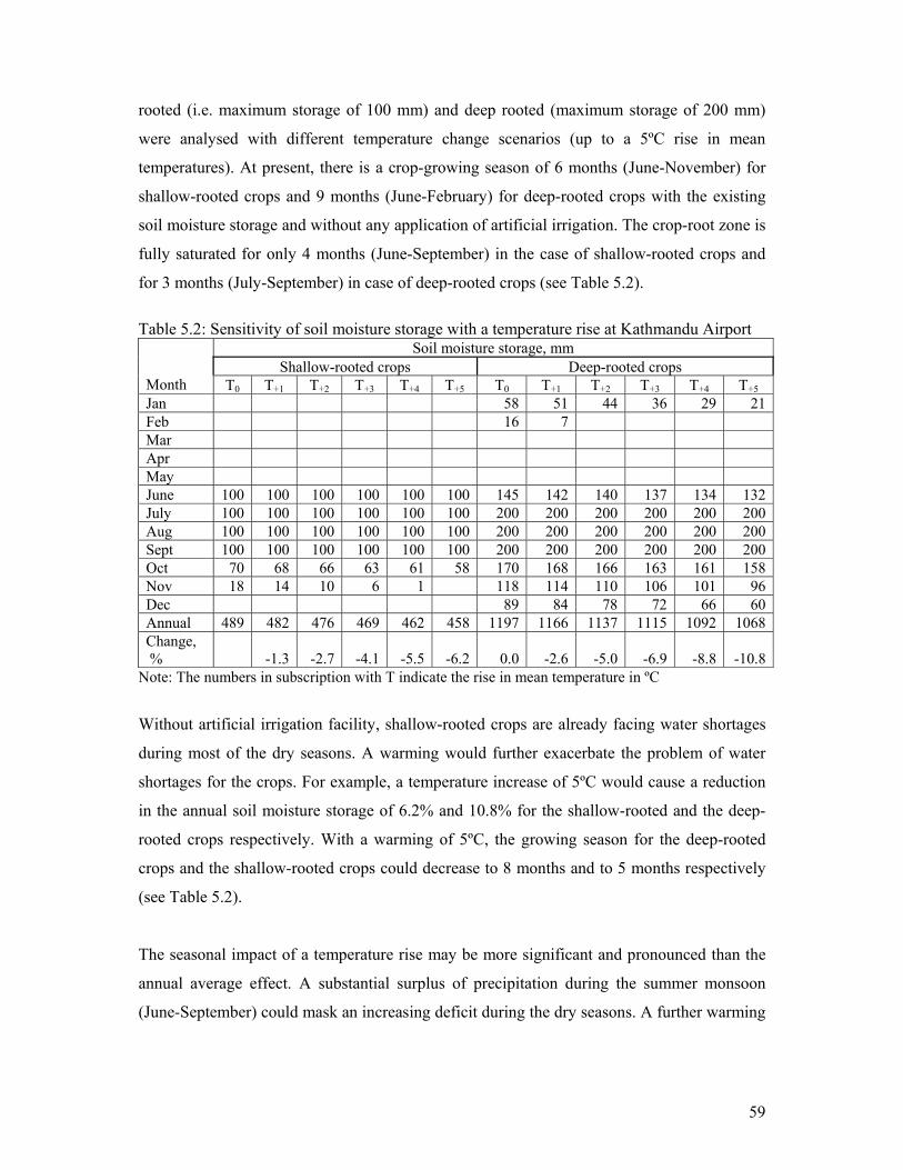
59
rooted (i.e. maximum storage of 100 mm) and deep rooted (maximum storage of 200 mm)
were analysed with different temperature change scenarios (up to a 5ºC rise in mean
temperatures). At present, there is a crop-growing season of 6 months (June-November) for
shallow-rooted crops and 9 months (June-February) for deep-rooted crops with the existing
soil moisture storage and without any application of artificial irrigation. The crop-root zone is
fully saturated for only 4 months (June-September) in the case of shallow-rooted crops and
for 3 months (July-September) in case of deep-rooted crops (see Table 5.2).
Table 5.2: Sensitivity of soil moisture storage with a temperature rise at Kathmandu Airport
Soil moisture storage, mm Shallow-rooted crops Deep-rooted crops
Month T0 T+1 T+2 T+3 T+4 T+5 T0 T+1 T+2 T+3 T+4 T+5 Jan 58 51 44 36 29 21Feb 16 7 Mar Apr May June 100 100 100 100 100 100 145 142 140 137 134 132July 100 100 100 100 100 100 200 200 200 200 200 200Aug 100 100 100 100 100 100 200 200 200 200 200 200Sept 100 100 100 100 100 100 200 200 200 200 200 200Oct 70 68 66 63 61 58 170 168 166 163 161 158Nov 18 14 10 6 1 118 114 110 106 101 96Dec 89 84 78 72 66 60Annual 489 482 476 469 462 458 1197 1166 1137 1115 1092 1068Change, % -1.3 -2.7 -4.1 -5.5 -6.2 0.0 -2.6 -5.0 -6.9 -8.8 -10.8
Note: The numbers in subscription with T indicate the rise in mean temperature in ºC
Without artificial irrigation facility, shallow-rooted crops are already facing water shortages
during most of the dry seasons. A warming would further exacerbate the problem of water
shortages for the crops. For example, a temperature increase of 5ºC would cause a reduction
in the annual soil moisture storage of 6.2% and 10.8% for the shallow-rooted and the deep-
rooted crops respectively. With a warming of 5ºC, the growing season for the deep-rooted
crops and the shallow-rooted crops could decrease to 8 months and to 5 months respectively
(see Table 5.2).
The seasonal impact of a temperature rise may be more significant and pronounced than the
annual average effect. A substantial surplus of precipitation during the summer monsoon
(June-September) could mask an increasing deficit during the dry seasons. A further warming

60
could exacerbate the water stress especially during the dry seasons, which are already facing
a moisture deficit.
5.1.2 Discussion about the Impacts on Evapotranspiration and Moisture Balance
Rising temperatures increase evaporation from land surfaces and water bodies, which could
increase atmospheric water content. Increasing water vapour in the atmosphere could enhance
the greenhouse-gas effect and thereby could cause a further rise in the global temperature
(Mirza and Dixit, 1997, p.75). Higher temperatures and reduced snow cover can cause
reduced soil moisture (IPCC, 2001a, p.199). Increased evaporation could increase the
moisture deficit and could reduce the ground water recharge that may adversely affect the
river runoff. Additionally, increased evaporation and decreased soil moisture might result in
an increased demand on water for irrigation. Without any modern irrigation facilities, a
reduction in soil moisture storage can cause a shortening of the growing season for the
agricultural land (Vinnikov, 1992, p.126). Increased temperatures may widen the gap
between demand and supply of irrigation water, which could have a direct impact on the
agricultural production and the farming activities.
5.2 Impacts on the River Flows There are apparent differences in flow patterns between rain-fed and glacier-fed rivers. The
climate of Nepal is dominated by the monsoon. The runoff of the rain-fed rivers is only due
to precipitation, whereas that of the glacier-fed rivers consists of glacier-melt as well.
Analysis of the long-term river runoff data from both the Langtang and Bagmati basins
showed a visible difference in variations of monthly hydrographs between the glacier-fed
Langtang Khola and the rain-fed Bagmati River (see Figure 5.2) despite the variations in
monthly precipitation for both cases being almost the same (see Table 5.3). For example, the
ratios of maximum to minimum monthly precipitation for the Langtang and for the Bagmati
were 43 and 45 respectively, while the ratios of maximum to minimum monthly discharge for
the same were 6 and 34.5 respectively. The snow and glacier melt component most probably
has helped maintain a sustained flow in the glacier-fed river even during the non-rainy
seasons.

61
Figure 5.2: Comparative mean monthly hydrographs
0
50
100
150
200
250
300
Jan
Feb
Mar
Apr
May Ju
n
Jul
Aug Sep
Oct
Nov
Dec
Spec
ific
runo
ff, m
mGlacierfed Langtang
Rainfed Bagmati
Data source: DHMN; Graph by author
The Figure 5.2 clearly illustrates that there is a greater variability of flows, i.e. higher
likelihood of floods and droughts in the rain-fed Bagmati River than in the glacier-fed
Langtang Khola. The hydrograph of the present glacier-fed rivers may take the shape of that
of the rainfed rivers in the future after the glaciers disappear due to a temperature rise.
Therefore, it is likely that disappearance of glaciers will enhance the variability of flows.
Table 5.3: Precipitation and river runoff of the Langtang Khola and the Bagmati River
Basin Jan Feb Mar Apr May Jun Jul Aug Sep Oct Nov Dec
A 17.2 17.2 23.0 23.1 33.2 74.2 112.0 163.4 82.2 15.2 7.8 3.8 P,
mm B 13.7 17.4 30.3 56.9 116.3 261.6 356.5 319.6 186.9 56.7 7.9 15.1
A 23.8 20.5 23.5 22.2 39.2 99.2 123.3 120.8 89.0 50.2 30.6 23.8 q,
mm B 11.5 7.7 7.1 7.9 11.3 64.4 207.8 244.6 156.9 75.1 30.9 17.8
Note: P= Precipitation; q= Specific runoff; A= Glacier-fed Langtang; B= Rain-fed Bagmati
The rain-fed river has the highest flow in August whereas the glacier-fed river has the highest
flow in July because there is a significant melt-water component in the glacier-fed river. Any
changes in precipitation and temperature may have a direct impact on the runoff pattern and
the water balance of the whole river system.

62
5.2.1 Runoff Modelling of the Bagmati River at Chovar
In order to detect the impacts of climate changes on river flows, the water balance model
WatBal was applied at the Chovar hydrological station of the Bagmati River. The Bagmati
River is one of the major rain-fed rivers of Nepal, which originates at Shivpuri in the north
east corner of the Kathmandu Valley at about 2760 metres above sea level (masl). The river
crosses the capital city of Kathmandu, currently experiencing the highest population pressure
in Nepal. It passes through the middle mountains, mid-hills and low plain areas down to the
Nepal-India border at about 73 masl. The hydrological station Chovar of the Bagmati River is
located at an altitude of 1280 masl with a catchment area of 585 km2. The average monthly
hydrological and meteorological data, viz. river flow, temperature, precipitation, relative
humidity, sun shine hours and wind speed were used as the input variables for calibration and
validation of the model. The hydrologic data observed by the Chovar station (DHMN Index
No 550) and meteorological data by the Kathmandu Airport station (DHMN Index No 1030)
were included in the model calibration and validation. The model was calibrated with the
observed data for 60 months (1971-1975). The model parameters identified during the
calibration were validated with the data for another 60 months (1976-1980). The input data
and identified model parameters are:
Input data Correlation coefficient Error, mm
Calibration 1976-1980 0.93 916
Validation 1971-1975 0.91 2376
Subsurface runoff coefficient (SSRC), α = 136.5 Base flow = 4.03 mm/month
Surface runoff (SRC), ε = 4 Direct runoff coefficient = 0.005
Initial storage, Zi = 0.15 Maximum storage, Smax= 624 mm
Temperature changes: +1ºC to +5ºC Precipitation changes: -10% to +10%
The model outputs have revealed that the modelled and observed runoff values are quite
comparable except for peak flood months (see Figure 5.3a, Annex 4.3).

63
Figure 5.3a: Modelling of the Bagmati River Runoff at Chovar (1976-80)
0
50100
150
200
250300
350
400
1 6 11 16 21 26 31 36 41 46 51 56
Months
Run
off,
mm
Modelledobserved
After identifying the model parameters, a sensitivity analysis was carried out by changing the
temperature and the precipitation in order to detect impacts of the temperature and
precipitation changes on the river runoff. The temperatures were changed from T+1 (i.e.
temperature rise of 1ºC) to T+5 (i.e. temperature rise of 5ºC) and precipitation from P-10 (i.e.
precipitation decrease of 10%) to P+10 (i.e. precipitation increase of 10%) (see Table 5.4).
Table 5.4: Sensitivity of the river runoff to climate change at the Chovar station Change in Runoff, %
T0 T+1 T+2 T+3 T+4 T+5 P-10 -11.6 -13.9 -14.7 -15.5 -17.0 -17.4 P-5 -5.7 -8.0 -9.5 -11.0 -11.4 -14.0 P0 0 -1.5 -2.8 -4.4 -5.8 -7.5 P+5 6.6 5.1 3.5 2.1 0.1 -1.1 P+10 13.6 12.0 10.4 8.8 7.2 3.6
Note: The subscriptions of T & P denote the changes in temperature (ºC) & precipitation (%)
The results in Table 5.4 show that the runoff has a negative correlation with temperature
change but a positive correlation with precipitation change. There will be a 7.5% decrease in
annual runoff with a 5ºC rise in the temperature assuming no change in precipitation.
Similarly, a 10% decrease in the precipitation and a 5ºC rise in the temperature may result in
a 17.4% decrease in the river runoff of the Bagmati River at Chovar.

64
5.2.2 Runoff Modelling of the Langtang Khola at Langtang
After modelling the runoff of the rain-fed Bagmati River, the runoff modelling was made
with WatBal model for the glacier-fed Langtang Khola too. The Langtang Khola is one of the
very few glacier-fed rivers with continuous hydrological data since 1988 in the Nepal
Himalayas. The hydrological as well as meteorological data for modelling were obtained
from the Snow and Glacier Hydrology Unit of the Department of Hydrology and
Meteorology in Nepal, which were recorded at the Langtang (Kyangjing) station. The model
was calibrated with the observed data for 72 months (1993-98) and validated with the data for
another 60 months (1988-1992). The basin area upstream of the modelling site is 340 km2,
out of which 142 km2 is currently covered by glaciers. About 61% of the total basin area is
located above 5000 masl. The altitude of the Langtang hydrological station is 3800 masl. The
highest point within the basin is at 7232 masl. The input data and identified model parameters
are as following:
Input data Correlation coefficient Error, mm
Calibration 1993-1998 0.84 508
Validation 1988-1992 0.74 968
Subsurface runoff coefficient, α = 19.04 Base flow = 15.2 mm/month
Surface runoff (SRC), ε = 0.14 Direct runoff coefficient (DRC) = 0.005
Initial storage, Zi = 0.5 Maximum storage, Smax= 81 mm
Temperature changes: +1ºC to +5ºC Precipitation changes: -10% to +10%
The model output is given in Figure 5.3a (see also Annex 4.4).
Figure 5.3b: Runoff Modelling of the Langtang Khola at Langtang (1993-98)
02040
6080
100120
140160
1 6 11 16 21 26 31 36 41 46 51 56 61 66 71Months
Run
off,
mm
Modelledobserved

65
A sensitivity analysis for the Langtang Khola was carried out for the temperature changes
from +10C to +50C and the precipitation changes from -10% to +10% (see Table 5.5).
Table 5.5: Sensitivity of the Langtang Khola runoff to climate change at Langtang Change in Runoff, %
T0 T+1 T+2 T+3 T+4 T+5 P-10 -6.4 -6.8 -6.9 -7.0 -7.1 -7.4 P-5 -1.9 -2.1 -2.3 -2.9 -3.5 -4.2 P0 0 -0.2 -0.3 -0.4 -0.5 -0.6 P+5 3.6 2.4 2.3 2.2 1.9 1.6 P+10 6.2 5.2 4.0 3.2 2.2 1.9
Note: The subscriptions of T & P denote the changes in temperature (ºC) & precipitation (%)
5.2.3 Synthesis of the Runoff Modelling of the Bagmati River and the Langtang Khola
The data in Table 5.5 show that the runoff of the Langtang Khola is less sensitive to
temperature rise than that of the Bagmati River (see Table 5.4). This is because of the
existence of the melt-water component in the runoff of the Langtang Khola, which masks the
effect of decreasing runoff due to warming by providing additional runoff from glacier-melt.
Therefore, there will be only a 0.6% decrease in annual runoff with a 5ºC rise in the
temperature assuming no change in the precipitation. Similarly, a 10% increase in the
precipitation and a 5ºC rise in the temperature may result in only a 1.9% increase in the
annual runoff of the Langtang Khola (see Table 5.5).
The climate of Nepal is highly dominated by the monsoon. The data presented in Table 5.3
shows that the monsoon season (i.e. June-September) contributes more than three quarters to
the annual precipitation (e.g. about 76% in the Langtang and about 78% in the Bagmati).
Because of this uneven distribution of precipitation and subsequently uneven distribution of
the river runoff, Nepal is already facing water shortages during the non-monsoon seasons and
flood problems during the monsoon season. The impacts of climate change will further
exacerbate the problem of uneven distribution of the river runoff. For example, a temperature
rise of 4ºC and a precipitation decrease of 10% will result in 17% and 7.1% decreases in
annual runoff in the Bagmati River and the Langtang Khola respectively (see Table 5.4 and
Table 5.5).
An analysis of the seasonal distribution of changes in river runoff due to climate change was
carried out for the whole scenarios of temperature rises from 1ºC to 5ºC rise (i.e. T+1 to T+5)

66
and precipitation changes from 10% decrease to 10% increase (i.e. P-10 to P+10) at Chovar of
the Bagmati River. The findings of the sensitivity analysis of the river runoff to temperature
change assuming no precipitation change at the Chovar reveal that sensitivity of the runoff to
a temperature change will vary among the months, and the river runoff during the non-
monsoon season (i.e. dry months) is more sensitive to warming (see Figure 5.4; Annex 5.4).
For example, a temperature rise of 5ºC will cause a decrease in March-runoff of 14.3%, but it
will cause a decrease in August-runoff only of 5.6%.
Figure 5.4: Sensitivity of monthly runoff of the Bagmati River to temperature change at Chovar
-16
-14
-12
-10
-8
-6
-4
-2
0Jan Feb Mar Apr May Jun Jul Aug Sep Oct Nov Dec
Cha
nge
in R
unof
f, %
T+1Po
T+2PoT+3Po
T+4PoT+5Po
Similarly, a sensitivity analysis of the river runoff to the precipitation change assuming no
temperature change was carried out. This analysis revealed that an increase in the
precipitation would substantially affect the monsoon runoff. For example, a precipitation
increase of 10% would cause an increase in July-runoff of 28.5% but only a 4.7% increase in
January-runoff assuming no change in temperature (see Figure 5.5; Annex 5.5). This
indicates that climate change would enhance the pronounced seasonality and the uneven
distribution of the runoff in the Nepalese rivers. The low flows (i.e. dry-season runoff) are
more sensitive to the temperature change whereas wet season flows (i.e. flood flows) are
more sensitive to precipitation change (see Figures 5.4 and 5.5).

67
Figure 5.5: Sensitivity of the Bagmati River runoff to precipitation changes at Chovar
-20-15-10-505
101520253035
Jan Feb Mar Apr May Jun Jul Aug Sep Oct Nov DecCha
nge
in R
unof
f, %
ToP+5 ToP+10ToP-5 ToP-10
After detecting the seasonal disproportion of impacts on runoff of the Bagmati River, a
comparative analysis of the impacts of climate change on the river runoffs of the rain-fed
Bagmati River and the glacier-fed Langtang Khola was carried out (see Table 5.6).
Table 5.6: Sensitivity of monthly runoff with temperature and precipitation changes
Change in runoff, % T+2, P+10 T+2, P-10 T+4, P+10 T+4, P-10
Month
Langtang Bagmati Langtang Bagmati Langtang Bagmati Langtang BagmatiJan 4.1 0.2 -5.6 -20.0 1.2 13.9 -5.6 -30.5Feb 2.5 0.6 -3.6 -19.9 1.8 10.9 -3.8 -29.9Mar 2.7 1.6 -4.8 -19.3 2.0 6.8 -5.1 -27.8Apr 2.0 4.0 -5.5 -17.3 1.6 1.6 -5.7 -23.2May 3.8 8.4 -8.3 -14.2 2.4 -3.7 -8.4 -15.7Jun 3.0 13.5 -4.3 -10.1 1.6 -6.6 -5.2 -6.4Jul 3.9 25.3 -7.3 -12.2 1.5 -2.4 -7.6 -10.5Aug 4.6 6.4 -7.3 -14.1 2.1 4.1 -7.6 -15.1Sep 4.9 3.0 -7.6 -15.5 2.6 9.1 -7.8 -20.4Oct 4.0 3.0 -9.9 -19.0 2.5 12.9 -9.4 -27.5Nov 5.1 1.2 -9.3 -22.8 5.9 17.5 -8.7 -34.7Dec 1.5 1.1 -0.5 -22.6 1.4 16.3 -0.4 -34.2Annual 3.9 10.8 -6.9 -15.4 2.2 3.8 -7.1 -16.9Note: The subscriptions of T & P denote the changes in temperature (ºC) & precipitation (%)
The results in Table 5.6 show an uneven distribution of the change in runoff among the
months despite a uniform change in precipitation and temperature in a particular scenario. For
example, a 2ºC rise in temperature and a 10% decrease in precipitation (T+2, P-10) will result
in 6.9% and 15.4% decreases in the annual runoff of the Langtang Khola and the Bagmati

68
River respectively (see Table 5.6). For an annual-runoff decrease of 6.9% under T+2, P-10
scenario, December-runoff will decrease by 0.5% whereas May-runoff will decrease by 8.3%
for the Langtang Khola. Similarly, for an annual decrease of 15.4% for the Bagmati River,
June-runoff will decrease by 10.1% whereas November-runoff will decrease by 22.8% for the
same scenario. These results clearly indicate that the problem of seasonal imbalance of river-
flows will be more exacerbated in the future with the temperature and precipitation change
scenarios.
The seasonal effect will be more pronounced for rain-fed rivers than for glacier-fed ones. In
case of the Bagmati River for the given scenario (T+2, P-10), the biggest changes will occur
during non-monsoon seasons. In case of the Langtang, there will be minimum decrease of
flows during dry seasons because there will still be the glacier-melt component masking the
warming effect (see Figure 5.6; Annex 5.6). The model WatBal itself assumed the snow- and
glacier area within the basin as constant and not variable at least for the present application,
which may not be true for increasing temperatures. Therefore, further assessment is necessary
to identify the possible impacts of temperature increase on the snow and glacier contribution
to the river flows.
Figure 5.6: Sensitivity of River Runoff to Climate Change (T+2, P-10 Scenario)
-25
-20
-15
-10
-5
0Jan Feb Mar Apr May Jun Jul Aug Sep Oct Nov Dec
Cha
nge
in r
unof
f, %
Langtang (glacier-fed) Bagmati (rain-fed)

69
5.2.4 Discussion of the Empirical Evidence on the Impacts on the River Flows
Mirza and Dixit (1997, p. 78) reported that for an increase in temperature by 2ºC and increase
in precipitation by 10%, the runoff of the Ganges in Delhi might increase by 19%. By
simulating an integrated water balance model WatBal, Yates (1994, p.13) found out that for
an increase in temperature of 4ºC and an increase in precipitation of 10%, the runoff of the
Mulberry River in Arkansas and the East River in Colorado in USA would increase by 11%
and 4% respectively. Similarly, MOPE (2004, p.99) revealed using the WatBal model that for
an increase in temperature of 4% and an increase in precipitation of 10%, the runoff in the
Karnali, the Narayani, the Koshi and the Bagmati Rivers in Nepal would increase by 1%, 9%,
5% and 11% respectively. The simulation of the WatBal model in the current study revealed
that for an increase of temperature of 4ºC and an increase in precipitation of 10%, the runoff
in the Bagmati River at Chovar and the Langtang Khola at Langtang would increase by 3.8%
and 2.2% respectively. The findings of the current study, thus, support the results of the
previous studies.
Recently, Shrestha (2005, p.75) reported that the annual river runoff of the Kali Gandaki
River at Kotagaun in western Nepal was increasing by approximately 1% per year. The snow
area upstream of the station within the basin is about 19% (WECS/DHMN, 1996, Annex-2),
which might have contributed a substantial percentage of melt-water to the annual runoff,
which may be the possible explanation for an increasing annual runoff. The low flows in the
rivers (during April-May) in the present study were found to be more sensitive to an increase
in temperature and a decrease in precipitation. Likewise, the high flows (during July-August)
were more sensitive to an increase in precipitation. Besides, the low flows in the rain-fed
Bagmati River were more sensitive to warming than those in the snow-fed Langtang Khola
due to the lack of the melt-water component in the rain-fed river during the dry period.
Climate change will significantly increase the intra-annual variability of stream flow
(Agrawala et al., 2003, p.29). This statement reinforced the findings of the current study. For
example, the range of flow (i.e. the difference between the highest and the lowest flows) of
the Bagmati River would increase from the present 268 m3/s (i.e. from 7.3 m3/s to 275.3 m3/s)
to 371.6 m3/s (i.e. from 6.9 m3/s to 379.6 m3/s) for a temperature rise of 4ºC and a
precipitation increase of 10%.

70
5.3 Impacts of a Temperature Rise on Snow and Glacier Systems 5.3.1 General Findings
To begin with, the information on the glaciers located upstream of the Langtang hydrological
station was collected from the topographical maps of Nepal (HMGN, 1997, Sheet Nos. 2885
10, 2885 11, 2885 14, 2885 15, Scale: 1:50 000) and the Inventory of Glaciers in the Nepal
Himalayas (ICIMOD/UNEP, 2002; Mool et al., 2001a, pp.224-225). The total area of the
study basin was 340 km2. There were altogether 24 glaciers with a total surface area of 140.8
km2 (about 41% of the total basin area) within the study basin (see Figure 5.7; Annex 5.8).
Figure 5.7: Basin area at Langtang
0
5
10
15
20
25
3800
4200
4600
5000
5400
5800
6200
6600
7000
Altitude, masl
Bas
in a
rea,
km
2 Non-glacierised areaGlacierised area
The highest and lowest altitudes within the basin were 7232 metres above sea level (masl)
and 3800 masl respectively. The glaciers were distributed from the lowest point of 4130 masl
to the highest point of 7218 masl. The smallest glacier was 0.01 km2 whereas the largest one
was 67.93 km2. The thickness of the glaciers also varied from 2.1 m to 177.3 m. Out of the 24
glaciers, the largest one alone had an ice reserve of 12.04 km3 (i.e. 63% of the total ice
reserve in the basin), and the second and the third largest ones had ice reserves of 3.32 km3
and 1.84 km3 respectively. The remaining 21 glaciers had altogether only 10% of the whole
ice reserve in the basin indicating that the majority of the glaciers were very small.

71
Figure 5.8: Average glacier mass balance with altitudes
-35
-30
-25-20
-15
-10
-5
05
10
15
3800
4200
4600
5000
5400
5800
6200
6600
7000
Altitude, masl
Gla
cier
mas
s, 1
06 m3 w
.e./a
AccumulationAblationBalance
The accumulation and ablation of the glaciers within the Langtang valley were calculated for
each month and for every 100 m altitude level from 3900 to 7218 masl by applying an
empirical relation. The temperatures and subsequently the glacier mass balance varied with
the altitudes and the months. The precipitation for the whole study basin was assumed to be
uniform over the whole study basin and taken as the same as recorded by the meteorological
station at Langtang (Kyangjing) located at 3920 masl. Though it may not be true for the
mountain topography of the study area, there were no other meteorological stations within the
basin to verify the assumption. As far as temperature data were concerned, the adiabatic lapse
rate (i.e. the rate of temperature change with altitude) was taken as -0.6ºC per 100 m of
altitude. The lapse rate was assumed to be the same for all altitude levels and for all months.
The total accumulation, ablation and glacier mass balance for each 100 m altitude level were
calculated by summing up all monthly values. The lower altitudes were dominated by
ablation whereas the upper ones by accumulation (see Figure 5.8, Annex 5.7). The
equilibrium line altitude, the altitude at which the accumulation and ablation of the glacier is
equal, was found at 5367 masl.

72
Figure 5.9: Monthly glacier mass balance at Langtang in m w.e./yr
-0.6
-0.5
-0.4
-0.3
-0.2
-0.1
0
0.1
0.2
Jan Feb Mar Apr May Jun Jul Aug Sep Oct Nov Dec
Spec
ific
mas
s ba
lanc
e,m
w.e
.
AccumulationAblationBalance
Jan Feb Mar Apr May Jun Jul Aug Sep Oct Nov Dec Yr Ac 0.04 0.04 0.05 0.05 0.07 0.11 0.14 0.20 0.12 0.03 0.02 0.01 0.87Ab 0.02 0.02 0.03 0.03 0.13 0.38 0.53 0.51 0.30 0.04 0.01 0.00 1.98Bl 0.02 0.02 0.03 0.02 -0.06 -0.27 -0.39 -0.31 -0.18 0.00 0.01 0.00 -1.11
Note: Ac= Accumulation; Ab = Ablation; Bl = Balance; Values are the averages of 1988-2000 and expressed in metres of water equivalent
There was wide a variation in glacier mass balance among the months. The total volume of
the glacier mass balance over the whole glaciers was obtained by summing up all glacier
mass balances of each altitude level. The total glacier mass balance in terms of volume of
water equivalent (w.e.) was further divided by the glacier area in order to get a specific mass
balance (see Figure 5.9). The calculated monthly specific mass balance of the glaciers shows
that there was a substantial negative glacier mass balance during the study period of 1988-
2000 in the Langtang Valley. The summer months (June-September) had substantial glacier
ablation despite some accumulation.
5.3.2 Sensitivity Analysis of Glacier Mass Balance to Temperature Rise
As the precipitation data during the past did not show any significant trends, a sensitivity
analysis of glacier mass balance and glacier-contributed runoff was carried out only for the
temperature change scenarios from T+1 to T+5 (i.e. temperature rise from 1ºC to 5ºC). Then,
the calculated values were compared with the T0-scenario (no temperature change). The
equilibrium line altitude (ELA) would move up to 6142 masl at T+5-scenario, whereas the
ELA at present (i.e. at T0-scenario) is located at 5367 masl (see Figure 5.10; Annex 5.9;
Annex 5.10).

73
Figure 5.10: Sensitivity of glacier mass balance in altitudes
-90-80-70-60-50-40-30-20-10
01020
3800
4200
4600
5000
5400
5800
6200
6600
7000
Altitude, maslM
ass
bala
nce,
106 m
3 /yr
T0T+1T+2T+3T+4T+5
A temperature increase will not only impact the annual glacier mass balance, but will also
change the precipitation pattern. Even without any change in total annual precipitation, more
precipitation will occur in a liquid form (i.e. rainfall) instead of a solid form (i.e. snowfall)
with warmer temperatures. Rainfall, unlike snowfall, will not be stored, but will immediately
be drained out from the basin resulting in more floods downstream during the monsoon. The
impact of a temperature rise could easily be visible in the sensitivity analysis through snow-
to-rain ratio, glacier mass balance rate or life of glacier ice reserve. For example, the snow-to-
rain ratio would decrease from 1.6 to 0.5, the life of ice reserves would decrease from 110 to
25 years and the glacier mass balance would decrease from -1.114 to -4.850 m.w.e.yr-1 with
a warming of 4ºC (see Table 5.7). In order to assess the accuracy of the calculation of the
glacier mass balance, a theoretical runoff (QT) at the Langtang hydrological station was
compared with the measured runoff (QM). The theoretical runoff (QT) at the Langtang station
was calculated by the relation:
QT= P+Abl-Acc-E (5.1)
Where,
QT = Theoretical runoff, 106 m3 yr-1
P = Precipitation, 106 m3 yr-1
Abl = Glacier Ablation, 106 m3 yr-1
Acc = Glacier Accumulation, 106 m3 yr-1
E = Total evaporation, 106 m3 yr-1

74
Therefore, QT = (199+279-122.6-138.0) 106 m3 yr-1 = 217.4 x 10⁶ m3 yr-1. The observed annual
average runoff (QM) at the Langtang hydrological station (Kyangjing) for the period of 1988-
2000 was 218 x 106 m3 yr-1, which gave an error of less than 1% level for the calculation.
Likewise, the results showed that even without any changes in the precipitation amount, a
warming of 5ºC would cause a decrease in snowfall of 55.6% and an increase in rainfall of
89.2% simultaneously. The analysis further revealed that glaciers in the Langtang valley were
already melting so rapidly that even without any further warming they would disappear in 11
decades from 2001, if the present rate of melting continues. With a warming of 2ºC, all the
glaciers with a present ice reserve of 19.14 km3 would disappear within less than half a
century (see Table 5.7). A further calculation was done in order to quantify a glacier mass
balance rate for a particular warming rate instead of the total amount of warming.
Table 5.7: Summary of sensitivity analysis of glaciers at Langtang (1988-2000) Temperature Change Scenarios Parameters Unit
T0 T+1 T+2 T+3 T+4 T+5 Precipitation
106 m3 yr-1 199.0 199.0 199.0 199.0 199.0 199.0
Snowfall
106 m3 yr-1 122.6 (0)
108.6 (-11.4)
93.5 (-23.7)
79.0 (-35.5)
66.6 (-45.7)
54.4 (-55.6)
Rainfall
106 m3 yr-1 76.4 (0)
90.4 (18.2)
105.5 (38.1)
120.0 (57.0)
132.4 (73.3)
144.6 (89.2)
Snow-to-rain ratio
1.60 1.20 0.89 0.66 0.50
0.38
Evaporation
106 m3 yr-1 138.0 (0)
142.8 (3.5)
147.7 (7.0)
152.6 (10.6)
157.6 (14.2)
162.7 (17.9)
Ablation
106 m3 yr-1 279.0 351.6 463.6 596.9 750.8
925.7
Accumulation
106 m3 yr-1 122.6 108.6 93.5 79.0 66.6
54.4
Total mass balance
106 m3 yr-1 -156.8 -242.8 -369.5 -516.7 -683.0
-870.5
Specific mass balance*
m w.e yr-1 -1.114 -1.724 -2.623 -3.668 -4.850
-6.181
Life of ice reserve
year 110 71 47 33 25
20
Note: * Specific glacier mass balance is the mass balance of the studied glaciers over the unit surface area expressed in meters of water equivalent (m w.e.).
- Values in subscription with T indicate an increase in temperature in ºC - Values in the parentheses show a percentage change from the T0-scenario

75
The regression analysis between an increase in temperature and a glacier mass balance
revealed the empirical relation given in Equation 5.2 (p<0.001; R2=1.0)
∆B = -0.6087*∆T1.3117 (5.2)
Where,
∆B = Change in glacier mass balance in m.w.e.yr-1
∆T= Change in temperature in ºC
Using the relation, glacier mass balance rates for the next 20 decades from 2001 were
calculated (see Table 5.8). The mass balance rates were calculated using the output values
from Table 5.7 for different scenarios of temperature rise and then converted to the rate of
warming using the Equation 5.2. For example, the negative glacier mass balance rate for the
T0-scenario was taken as the same as the average calculated value for the period of 1988-
2000. The negative glacier mass balance rates for the warming rates of 0.03ºC yr-1 to 0.15ºC
yr-1 (i.e. T+0.03, T+0.06,…, T+0.15-scenarios) for every decade were calculated by:
BTx,n = BT0,n + ∆Bx,n (5.3)
Where,
BTx,n = Glacier mass balance rate for n-decade with a warming rate of x
( Here, x = 0, 0.03, 0.06, 0.09, 0.12 , 0.15 ºC/yr; n=0,1,2,…, 20)
BT0,n = Glacier mass balance rate for n-decade without a further warming
∆Bx,n = Change in glacier mass balance rate for n-decade with a warming rate of x
Then, all values of the specific glacier mass balance for every temperature rise scenario and
for each decade were calculated (see Table 5.8). The decades were counted from 2001, e.g.
decade-0 means 2000, decade-1 means 2010, decade-3 means 2030…, and so on. The
calculated specific glacier mass rates given in Table 5.8 were applied to all the existing
glaciers in the Nepal Himalayas in order to carry out a sensitivity analysis of the total glacier
ice reserve of 480.6 km3 to a temperature rise (see Table 5.9). The glacier-ice reserve of each
glacier was calculated by:
Vx,n =Vx,n-1 + Bx,n * An (5.4)
Where,
Vx,n = Volume of glacier-ice reserve in n-year for a warming rate of x [m3]
Vx,n-1 = Volume of glacier-ice reserve in n-1 year for a warming rate of x [m3]
Bx,n = Specific glacier mass balance in n-year for a warming rate of x [m w.e./yr]
An = Surface area of the particular glacier in n-year [m2]

76
Table 5.8: Glacier mass balance rates with different temperature change scenarios Specific glacier mass balance, m.w.e./year Decade
∆T = 0ºC/yr
∆T = 0.03ºC/yr
∆T = 0.06ºC/yr
∆T =0.09ºC/yr
∆T =0.12ºC/yr
∆T =0.15ºC/yr
0 -1.114 -1.114 -1.114 -1.114 -1.114 -1.1141 -1.114 -1.239 -1.425 -1.644 -1.887 -2.1502 -1.114 -1.425 -1.887 -2.430 -3.033 -3.6853 -1.114 -1.644 -2.430 -3.353 -4.380 -5.4914 -1.114 -1.887 -3.033 -4.380 -5.878 -7.4985 -1.114 -2.150 -3.685 -5.491 -7.498 -9.6696 -1.114 -2.430 -4.380 -6.674 -9.223 -11.9807 -1.114 -2.724 -5.112 -7.920 -11.040 -14.4158 -1.114 -3.033 -5.878 -9.223 -12.940 -16.9619 -1.114 -3.353 -6.674 -10.577 -14.916 -19.609
10 -1.114 -3.685 -7.498 -11.980 -16.961 -22.35011 -1.114 -4.028 -8.348 -13.427 -19.072 -25.17812 -1.114 -4.380 -9.223 -14.916 -21.243 -28.08713 -1.114 -4.742 -10.120 -16.444 -23.471 -31.07414 -1.114 -5.112 -11.040 -18.009 -25.754 -34.13215 -1.114 -5.491 -11.980 -19.609 -28.087 -37.26016 -1.114 -5.878 -12.940 -21.243 -30.470 -40.45317 -1.114 -6.272 -13.919 -22.909 -32.900 -43.70918 -1.114 -6.674 -14.916 -24.606 -35.375 -47.02519 -1.114 -7.082 -15.930 -26.332 -37.893 -50.40020 -1.114 -7.498 -16.961 -28.087 -40.453 -53.830
Note: decades are counted from 2001
The total glacier-ice reserve in the Nepal Himalayas for a particular year was obtained by
summing up the ice reserve of all existing glaciers for the same year. The summary of the
results (see Table 5.9, Figure 5.11) shows that the glacier-ice reserve will substantially be
decreasing and the rate of reduction will increase with the rate of warming.
Figure 5.11: Sensitivity of glacier-ice reserve to a warming
0
100
200
300
400
500
600
0 5 10 15 20Decade
Gla
cier
-ice
rese
rve,
km
3 T=0 degC/yrT=0.03 degC/yrT=0.06 degC/yrT=0.09degC/yrT=0.12degC/yrT=0.15degC/yr

77
Even without any further warming, there will be only 54.8 km3 of glacier-ice reserve left by
the year 2100, which is only 11.4% of the present glacier-ice reserve of 480.6 km3. Even if
the temperature stops rising and the current rate of melting continues, there will be no glacier-
ice reserve left by the year 2180. Temperatures in the Nepal Himalayas are increasing by at
least 0.06ºC/year (Shrestha, 1999, p.2775), which would further accelerate the glacier melt. If
the temperature further rises at this rate (i.e. 0.06ºC/year), there will be no glacier-ice reserve
left in the Nepal Himalayas by the year 2070.
Table 5.9: Sensitivity of glacier ice-reserve to a temperature rise in Nepal
Glacier ice-reserve, km3 Decade ∆T
= 0ºC/yr ∆T
= 0.03ºC/yr ∆T
= 0.06ºC/yr ∆T
=0.09ºC/yr ∆T
=0.12ºC/yr ∆T
=0.15ºC/yr 0 480.6 480.6 480.6 480.6 480.6 480.61 421.1 417.8 413.0 407.3 400.9 394.02 361.6 347.1 325.8 301.3 275.0 248.33 303.6 270.0 224.7 178.3 135.3 97.04 250.2 195.3 130.4 74.4 34.8 11.25 203.3 129.4 56.3 14.1 0.0 0.06 163.0 74.5 13.3 0.0 0.0 0.07 128.8 35.1 0.0 0.0 0.0 0.08 99.4 11.0 0.0 0.0 0.0 0.09 74.8 0.6 0.0 0.0 0.0 0.0
10 54.8 0.0 0.0 0.0 0.0 0.011 39.0 0.0 0.0 0.0 0.0 0.012 26.8 0.0 0.0 0.0 0.0 0.013 16.8 0.0 0.0 0.0 0.0 0.014 10.1 0.0 0.0 0.0 0.0 0.015 5.6 0.0 0.0 0.0 0.0 0.016 2.2 0.0 0.0 0.0 0.0 0.017 0.2 0.0 0.0 0.0 0.0 0.018 0.0 0.0 0.0 0.0 0.0 0.0
Note: decades are counted from 2001
The value of Equation 5.4 for a particular glacier would become negative, when the existing
glacier-ice reserve is less than the melt potential for the particular year. If that happened, the
particular glacier would be considered as disappeared. The areas of the remaining glaciers
were summed up for the total glacier areas (see Figure 5.12 and Annex-5.1)

78
Figure 5.12: Sensitivity of glacier surface area to a warming
0
1000
2000
3000
4000
5000
6000
0 5 10 15 20Decade
Gla
cier
are
a, k
m2T=0 degC/yr
T=0.03 degC/yr
T=0.06 degC/yrT=0.09degC/yr
T=0.12degC/yr
T=0.15degC/yr
The Figure 5.12 shows that the current glacier-cover will be reduced by 70% even without
any further warming in 2100. If the rate of temperature rise is 0.06ºC/year, the glacier areas
will be reduced by 70% by the year 2050.
Figure 5.13: Distribution of glaciers with areas in Nepal (2001)(Source: Mool et al., 2001a, pp.210-292)
> 10 km2
3%1-10 km2
24.4%
0.1-0.5 km2
42%0.5-1km2
18%
< 0.1km2
13%
Currently, there are 3252 glaciers in the Nepal Himalayas. About 72.6% of them are with
surface areas less than 1 km2 (see Figure 5.13). The sensitivity analysis shows that about 86%
of the glaciers in the Nepal Himalayas will disappear by 2050 even without any further
warming. If there is a warming of 0.06ºC/year, about 98.5% of the glaciers will disappear by
2050 and there will be no glacier left by 2070 (see Figure 5.14 and Annex 5.2).

79
Figure 5.14: Sensitivity of glaciers to a warming in Nepal
0
500
1000
1500
2000
2500
3000
3500
0 5 10 15 20Decade
Num
ber
of g
laci
ers
T=0 degC/yrT=0.03 degC/yrT=0.06 degC/yrT=0.09degC/yrT=0.12degC/yrT=0.15degC/yr
The projected disappearance of the glaciers in the Nepal Himalayas will undoubtedly reduce
the contribution of glacier-melt water to the total water availability. Currently, glacier-melt
water amounts to 4% of the total surface runoff of 176.08 km3. The glacier-melt contribution
will be higher for a higher rate of warming. For example, glacier-melt water will reach its
maximum of 15.32 km3/year in 2040, if the warming rate is 0.06ºC/year. Likewise, it will
reach its maximum of 20.21 km3/year in 2030, if the warming rate is 0.12ºC/year. The
glacier-melt contribution will be substantially reduced after its maximum because there will
be fewer glaciers left to melt (see Figure 5.15, Annex 5.3). As the contribution of glacier-melt
decreases, the total water availability of Nepal will decrease accordingly.
Figure 5.15: Sensitivity of glacier-melt water to a warming
0
5
10
15
20
25
0 5 10 15 20Decade
Gla
cier
-mel
t wat
er, k
m3 /a T=0 degC/yrT=0.03 degC/yrT=0.06 degC/yrT=0.09degC/yrT=0.12degC/yrT=0.15degC/yr

80
Total water availability depends not only on the glacier-melt contribution, but also on the
evapotranspiration losses. Increasing temperatures may further reduce the total water
availability even after the glacier-disappearances because of a possible increase in
evapotranspiration associated with the rising temperatures. The total water availability in
Nepal will decrease by 2.4% in 2100 even without any further warming (see Figure 5.16,
Annex 5.4). If there is warming rate of 0.06ºC/year, the total water availability may decrease
by 15% in 2100 and by 27% in 2200 from the level in 2001. A greater rate of warming might
cause an accelerated decrease in the total water availability. For example, if there is a
warming rate of 0.12ºC/year, the total water availability in Nepal may decrease by 27% in
2100 and by 51% in 2200 (see Annex 5.4).
Figure 5.16: Sensitivity of total water availability to a warming
020406080
100120140160180200
0 5 10 15 20
Decade
Wat
er a
vaila
bilit
y, k
m 3
/a
0ºC/yr 0.03ºC/yr0.06ºC/yr 0.09ºC/yr0.12ºC/yr 0.15ºC/yr
5.3.3 Discussion about the Impacts of Climate Change on Snow and Glaciers
Higher temperatures will increase the ratio of rain to snow, accelerate the rate of snowmelt
and shorten the overall snowfall (Frederick and Gleick, 1999, p.9). Changes in the snow
cover of the earth affect both daily weather and long-term climate (Walsh, 1984, p.50).
However, the feedback of the snow cover to the atmosphere is difficult to accurately quantify
due to the complex air-sea-land interactions (ibid, p.56). The most significant feedback is the
surface albedo or the reflectivity. Fresh snow has up to 85% of albedo that can reduce the
solar energy available to the surface and lower atmosphere by more than 50% (ibid, p.50).
Decrease in snow-to-rain ratio reduces the glacier accumulation even without any changes in

81
total precipitation. A decrease in snowfall accelerates the ablation due to a lowered albedo at
the glacier surface (Ageta and Kadota, 1992, p.89). Therefore, a decreasing snow cover and
an increasing ratio of rain-to-snow ratio due to warming may have an amplifying effect on
warming.
The Himalayas have a strong influence on the climate of the Indian subcontinent. It acts as a
climate divide between the north and south. Monsoon rain in the Indian subcontinent mostly
occurs due to the orographic influence of the Himalaya on the monsoon winds (Mani, 1981,
p.8). The Himalayan range obstructs the passage of extremely cold continental air from the
north into the subcontinent in the winter. In summer, it forces the rain-bearing monsoonal
winds to ascend and thereby give up most of their moisture as rain and snow on the south side
before crossing the range northward causing arid conditions in Tibet (ibid). Any changes in
temperature and thereby changes in snow cover affect the whole monsoon system. Khandekar
(1991, p. 644) reported that there existed a connection between the Eurasian snow cover, the
Indian monsoon and the El Niño/ Southern Oscillation phenomenon. Likewise, Dey and
Bhanu Kumar (1983, p. 5473) revealed an inverse relationship between the Himalayan snow
cover and the Indian summer monsoon rainfall.
Currently, about 10% of total annual precipitation in Nepal occurs as snowfall (UNEP, 2001,
p.129). Snow, glaciers and permafrost contribute about 10% to the annual stream flows in
Nepal (MOPE, 2004, p.95; Shrestha, 2005, p.76). There are currently 3,252 glaciers covering
a total surface area of 5,323 km2 with an estimated ice reserve of 481 km3 in the Nepal
Himalayas (Mool et al. 2001a, p.13). With a temperature increase of 1ºC, there will be a 20%
reduction in the present snow and glacier areas (MOPE, 2004, p. 96). The surface area of a
small glacier AX010 in the Shorong region of eastern Nepal decreased from 0.57 km2 in 1978
to 0.42 km2 in 1999 with an average shrinkage rate of 71 m2/yr (Fujita et al., 2001b, p.52).
The annual shrinkage rate of the glacier during 1978-91 was 50 m2/yr and increased to 200
m2/yr in 1996-99. The glacier was retreating by 50.9 m annually in 1998-99 (ibid). Asahi and
Watanabe (2000, p.481) reported after examining 57 glaciers in Kanchenjunga Himal, eastern
Nepal that most of them were retreating from 1958 to 1992. The net annual mass balance of
the glacier AX010 was -1.328 m w.e. in 1998, while that of the Rikha Sambha Glacier in
1999 was -0.732 m w.e. (WGMS, 2005, p.175). The calculated value of the average mass
balance rate of 24 glaciers in the Langtang Valley in the current study was -1.114 m w.e. (see

82
Table 5.7), which was within the range of the mass balance rates of other Himalayan glaciers
as mentioned before.
Recently, Brown (2006, p.68) reported that most of the glaciers in the world are shrinking
including the Himalayan glaciers. A study by a team of more than 50 US and Chinese
scientists over 26 years has reported that the glaciers in China are melting so rapidly that two
thirds of them will disappear by 2060, if the current melting rate continues (ibid, p.70). This
finding on the other side of the Himalayas has reinforced the findings of the present study
that the glaciers in the Nepal Himalayas are rapidly shrinking and will not last for a long, if
the current rate of melting continues.
As the warming continues, the volume of glaciers becomes smaller. This will result in the
decreased storage of fresh water in the mountains, which is vital for domestic use, irrigation
and hydropower for the people living not only in the mountains and but also far downstream
in the plains (Becker and Bugmann, 2001, p.63). An accelerated melting of glaciers on the
one hand and a decreasing snow-to-rain ratio on the other are two major impacts of warming
that may create additional liquid water in the mountains and may lead to the creation glacier
lakes in the mountain valleys. Many of these lakes are supported by loose moraines not
capable of resisting ever-increasing hydrostatic pressures caused by a rising lake-water level.
Therefore, a rising temperature will increase the likelihood of these lakes collapsing and
creating devastating flood disasters along a long stretch of the river valley downstream of the
lake, which is termed as Glacier Lake Outburst Flood (GLOF). A GLOF is a sort of debris
flow with great devastating power. The floodwater carries the debris from the collapsed dam,
erodes both banks and bed of the river and causes landslides from the steep slopes along the
river channel (Yamada, 1998, p.13). The damaging impacts of such debris flows may extend
even more than 100 km downstream causing substantial loss of lands, lives and properties.
However, damage magnitude of a GLOF depends on the volume of released water, rate of
water release, natural feature of the river channel and the status of infrastructure and
habitation in the likely-to-be-affected areas downstream (Yamada, 1998, p.14).

83
5.4 Conclusion 5.4.1 Summary of Findings
The analyses carried out in this chapter revealed that climate change would have a significant
impact on the atmospheric and soil moisture balance, the river runoff and the snow- and
glacier-regime causing a possible reduction on the total water availability in the Nepal
Himalayas. For example, the annual atmospheric moisture deficit will rise from 323 mm at
present to 413 mm under a temperature rise of 5ºC assuming no change in precipitation at
Kathmandu Airport. Likewise, the soil moisture storage for shallow- and deep-rooted crops
will drop by 6.2% and by 10.8% respectively at a temperature rise of 5ºC, and the crop-
growing season will also be shortened without an artificial irrigation. Similarly, a change in
climate will change the runoff regime of both glacier-fed and rain-fed rivers. The impact on
the runoff was found to be more pronounced for the rain-fed river, at least on a short-term,
because of the melt-water component existing in the runoff of the glacier-fed river. The
seasonal effect would be more serious than the annual effect due to domination of the
monsoon climate in Nepal. Climate change could cause an increased wet season runoff and a
decreased dry season runoff resulting in an increased seasonal variation in runoff.
A more remarkable impact of warming could be seen on the snow and glacier regime and on
the total water availability in the Nepal Himalayas. A warming could reduce the snow-to-rain
ratio, accelerate the glacier melt and increase the evaporation losses. For example, a 5ºC rise
in annual temperature in the Langtang Valley could reduce the snow-to-rain ratio from 1.6 to
0.38, increase the evaporation losses by 17.9% and shorten the estimated life of the glaciers
from 110 years to 20 years. The glaciers in the Nepal Himalayas are currently retreating so
rapidly that even without any further warming about 86% of the glaciers will disappear and
about 58% of the ice-reserve will be gone by 2050. If there is a warming of 0.06ºC/year, there
will be no glacier left in the Nepal Himalayas by 2070. Such a situation will substantially
reduce the total water availability in the Nepal Himalayas from 176.08 km3/year to 128.44
km3/year by 2200 at an assumed warming rate of 0.06ºC/year.
Such projected physical impacts on the water availability, moisture balance and runoff
variability will have a serious impact on the socio-economic development in Nepal.

84
5.4.2 Open Questions
The WatBal model, which was used in this study in order to identify the sensitivity of river
runoff to climate change, has used the average values of monthly precipitation, temperature
and runoff data, but not the extreme values. Therefore, further research is necessary to model
the extreme flows under the climate change. In addition, the effect of change in precipitation
pattern on the river runoff also could not be identified during the present study.
The determination of the impact of global warming on the glacier extent of the Nepal
Himalayas in this study was based on the assumption that all glaciers in the Nepal Himalayas
would be affected in the same way as in the Langtang valley. How accurate is this
assumption? Is the negative mass balance rate calculated in the Langtang valley
representative for the entire Nepal Himalayas? More studies covering other Himalayan
stations, which was beyond the scope of this study, are necessary to answer these questions.
In addition, the calculation of glacier mass balance in the Langtang valley was based on the
assumption that the precipitation data recorded at the Langtang (Kyangjing) station were
representative for the whole study basin of 340 km2. Because the mountain orography highly
influences the precipitation, this assumption needs to be verified by the future research.

85
Chapter VI: Empirical Findings on the Socio-economic Impacts
of Climate Change 6.0 General After quantifying the physical impacts of climate change in Nepal with reference to water
resources as discussed in chapter 5, the possible socioeconomic impacts of climate change
associated to these physical impacts are determined in this chapter. In particular, sensitivity
analyses of: 1. the irrigation water requirement, 2. the water balance situation, 3. the
agricultural production and the food security, 4. the hydropower potential, and 5. the water-
induced extreme events are carried out. At the end of this chapter, some conclusions and open
questions related to this chapter are presented.
6.1 Impacts on the Water Balance, Agriculture and Food Security 6.1.1 Impacts on the Irrigation Water Requirement
The existing irrigation water requirement was determined for the whole basin area upstream
of Chovar in the Bagmati river basin. The calculation was based on the information from the
water use inventory study carried out by the Water and Energy Commission Secretariat,
Nepal (WECS, 1997, Annex A-Table 5.1; WECS, 2000a, p.18). The specific irrigation water
requirement for each month was calculated by dividing the total water requirement with the
irrigated area inside the basin. The change in the irrigation water requirement due to factors
other than temperature rise was ignored during the analysis. The change in the irrigation
water requirement was assumed equivalent to the change in the potential evapotranspiration.
A sensitivity analysis of potential evapotranspiration in relation to a temperature rise for each
month at Kathmandu Airport was carried out using the FAO Penman-Monteith equation (see
Equation 3.14) for different temperature rise scenarios from T+1 (i.e. temperature change by
+1ºC ) to and T+5 (i.e. temperature change by +5ºC) for each month (see Table 6.1).

86
Table 6.1: Sensitivity of potential evapotranspiration to a temperature rise, 103m3/km2 T0 T+1 T+2 T+3 T+4 T+5 Jan 45.2 46.7 48.2 49.7 51.2 52.8 Feb 59.3 61.3 63.2 65.2 67.3 69.4 Mar 94.1 96.6 99.1 101.6 104.2 106.8 Apr 120.3 123.2 126.2 129.1 132.1 135.1 May 127.4 130.5 133.6 136.7 139.9 143.1 Jun 116.3 119.0 121.6 124.3 127.0 129.8 Jul 102.7 104.9 107.1 109.3 111.6 113.8 Aug 106.4 108.9 111.3 113.7 116.2 118.8 Sep 95.4 97.6 99.9 102.2 104.6 107.0 Oct 86.1 88.5 90.8 93.2 95.7 98.2 Nov 60.1 61.9 63.8 65.7 67.7 69.7 Dec 43.8 45.3 46.7 48.2 49.7 51.3 Annual 1057 1084 1111 1139 1167 1196 Absolute Change 27.0 54.3 82.0 110.1 138.6 Relative Change, % 2.6 5.1 7.8 10.4 13.1 Note: The numbers in the subscriptions with T denote the change in temperature in ºC.
The results shown in Table 6.1 reveal that an increase in temperature of 5ºC would cause an
increase in the annual potential evapotranspiration of 13.1%. Such an increase in the potential
evapotranspiration due to a temperature rise would increase the overall irrigation water
requirement. A sensitivity analysis of the irrigation water requirement (see Table 6.1) in
relation to a temperature rise has been calculated for the different temperature change
scenarios (T+1, T+2,…, T+5) by adding the extra potential evapotranspitation amount to the
original irrigation water requirement (i.e. with T0- scenario). During the analysis, the
influence of other non-climatic factors on the change in the irrigation water requirement was
not included (see Table 6.2).
The average specific annual water requirement for the irrigation at present (i.e. for T0-
scenario) has been calculated as 3,658,000 m3/km2 or 36,580 m3/ha. Generally, there are three
cropping seasons per year in most of the area within the basin. Rice is cultivated in the
biggest part of the irrigated area, even twice a year in most of the land. Maize, wheat and
vegetables are the other crops grown in the areas.

87
Table 6.2: Sensitivity of the irrigation water requirement to a warming, 103m3/km2 T0 T+1 T+2 T+3 T+4 T+5 Jan 111 118 126 133 141 149 Feb 148 157 167 177 187 198 Mar 112 125 138 150 163 176 Apr 58 73 87 102 117 132 May 35 50 66 81 97 113 Jun 790 803 816 830 843 857 Jul 401 412 423 434 445 457 Aug 171 183 195 207 220 232 Sep 240 251 262 274 286 298 Oct 621 633 644 657 669 681 Nov 896 905 915 924 934 944 Dec 76 83 91 98 106 114 Annual 3658 3793 3930 4068 4209 4352 Absolute Change 135 272 410 551 694 Relative Change, % 3.7 7.4 11.2 15.1 19.0 Note: The numbers in the subscriptions with T denote the change in temperature in ºC.
The results in Table 6.2 show that a 5ºC warming will increase the irrigation water demand
from 3.658 million m3/km2/yr to 4.352 million m3/km2/yr, i.e. a rise in demand of 19%.
6.1.2 Impacts on the Water Balance Situation
The existing water balance situation upstream of Chovar was determined based on the
demographic information and meteorological data within the basin. Available mean monthly
flows in the Bagmati river at Chovar were calculated using WECS approach and derived
from the publication of the WECS (1997, Table 3.4.1-b). The total irrigation water demand
was obtained for the total irrigated area of 105.6 km2 multiplying the values of specific
irrigation water demand from Table 6.2. The total domestic and industrial water demand was
identified according to the information about the rural and urban population within the basin.
Due to the lack of data on the actual water demand, the municipal water demand including
the industrial one for the urban area was assumed as 150 litres per capita per day (lpcd)
(WECS, 2000c, p.56). Similarly, rural water supply requirement including livestock demand
was assumed as 72 lpcd (ibid, p.46). The total rural and urban water supply requirement at
Chovar was then calculated for the current population of 1.48 million within the basin,
comprising of 509,446 rural and 975,645 urban residents (ISRSC, 2002, pp.228-256). The
municipal water demand was assumed to be uniform throughout the year. The irrigation
water demand was determined according to the crop water requirements and varied among

88
the months. The existing water supply and demand situation at Chovar clearly shows a
seasonal imbalance in the availability of water (see Figure 6.1).
Figure 6.1: Water Balance at Chovar (2001)
-40
-20
0
20
40
60
80
100
120
Jan
Feb
Mar
Apr
May Ju
n
Jul
Aug Sep
Oct
Nov
Dec
Dis
char
ge, m
3 /s
Available Use
Balance
As shown in Figure 6.1, five months of the year, namely January, February, March, June and
November already have a water deficit despite a sufficient surplus and a positive annual
water balance during the summer monsoon months from July to September (see Table 6.3). A
possible rise in temperature would further worsen the situation widening the gap between the
supply of and the demand for water, especially during the non-monsoon seasons. The effect
of climate change on the municipal water demand is relatively smaller than the effect of
economic development (IPCC, 2001b, p.211). Industrial water demand for processing
purposes is insensitive to climate change but it is defined by technologies and modes of use
(ibid). Irrigation water demand is considerably more sensitive to climate change. The
irrigation water use is the biggest factor (i.e. 96%) in the total annual water withdrawal in
Nepal (UNEP, 2001, p.122). Therefore, the municipal and industrial water demands were
assumed constant, the economic or population growth factors were excluded from the
analysis and only the irrigation water demand component of the total water balance was
considered sensitive to a temperature rise for the current analysis.

89
Table 6.3: Water supply and demand situation at Chovar in m3/s (2001) Water demand Month Water
supply Irrigation Municipal TotalWater balance
Jan 6.52 4.45 2.28 6.73 -0.21 Feb 6.42 5.93 2.28 8.21 -1.79 Mar 5.91 4.52 2.28 6.80 -0.89 Apr 6.45 2.33 2.28 4.61 1.84 May 9.19 1.40 2.28 3.68 5.51 Jun 27.41 31.75 2.28 34.03 -6.63 Jul 85.28 16.13 2.28 18.41 66.87 Aug 100.99 6.87 2.28 9.15 91.84 Sep 76.61 9.64 2.28 11.92 64.69 Oct 33.70 24.97 2.28 27.25 6.45 Nov 14.07 36.02 2.28 38.31 -24.24 Dec 9.13 3.06 2.28 5.35 3.78 Year 31.81 12.26 2.28 14.54 17.27
The change in temperature will change both the water supply and water demand. The
sensitivity of the river runoff was calculated through the WatBal Model in Chapter 5 (see
Table 5.4). An increase in temperature will result in a decrease in river discharge and an
increase in the water demand simultaneously, which ultimately widens the gap between the
river runoff and the water demand (see Figure 6.2). For example, a 5ºC rise in temperature
would cause an increase of the annual water demand of 19% and a reduction of the annual
river runoff of 7.5% at the same time.
Figure 6.2: Sensitivity of annual water balance situation at Chovar
3.7
7.4
11.2
15.1
19.0
-5.9
-7.5
-4.4
-3.0
-1.5
-10 -5 0 5 10 15 20 25
T+1
T+2
T+3
T+4
T+5
Tem
pera
ture
cha
nge,
0 C
Change, %Irrigation demandRiver runoff

90
Five months out of twelve are already facing water stress at Chovar. A temperature rise
would prolong the water deficit period and would further deteriorate the water balance
situation during the dry seasons despite enough surpluses during the rainy season. For
example, the number of months in a year with a water deficit would rise from five to nine and
the total annual water balance at Chovar will drop from 0.54 to 0.27 km3/year; if the
temperature increases by 5ºC (see Figure 6.3, Annex 6.1).
Figure 6.3: Change in Water Balance at Chovar
-35
-15
5
25
45
65
85
105
Jan
Feb
Mar
Apr
May Ju
n
Jul
Aug Sep
Oct
Nov
Dec
Wat
er B
alan
ce, m
3 /s
ToT+2T+4T+5
6.1.3 Impacts on the Agricultural Production, Food Security and Poverty
An increased irrigation water demand and a decreased river runoff due to warming would
have a substantial impact on the agricultural production. Agriculture is one of the sectors
most vulnerable to climate changes. Moreover, agriculture is one of the most important
sectors for Nepal’s socio-economic paradigm. About 81% of Nepal’s households have
agriculture as a major occupation (CBS, 2002, p.10). Agriculture currently occupies about
21% of Nepal’s land area (CBS, 2004a, p.41). The share of the agriculture in the gross
domestic product (GDP) of Nepal in 2004 was 39% (MOF, 2005, p.13). The agricultural
sector in 2002 provided 93% of the total labour force in Nepal (FAO, 2004a, p.1).
About 86% of Nepal’s population live in rural areas (ICRSC, 2002, p.20), where the
agricultural income contributes the largest share of household income. However, agriculture
remains predominately at subsistence level so far and is still largely non-commercialised. In

91
many of the rural mountain areas, agriculture income provides up to 90.4% of the total family
income (FAO, 2004b, p. 23). Export and import of the agricultural products provided only
14% and 16% of the total foreign trade in 2002 (FAO, 2004a, p.2). Therefore, foreign trade
will most likely have less effects of the reduction in agricultural products. In contrary, any
small changes on water supply and demand situations may have large impacts on the
livelihoods of the subsistence farmers although it may not be clearly visible in terms of the
GDP. Such a change in the water balance will disproportionately affect the poor because they
have less diversified sources of income and less knowledge and capacity to cope with the
changes.
The recent survey results on the status of poverty in Nepal revealed that nearly 31% of
Nepal’s population were currently living below the poverty line (MOF, 2005, p.150). The
definition of the poverty line was based on a minimum calorie requirement of 2144 kcal/day
for an average person. About 34.6% of rural and 9.6% of the urban population were under the
poverty line (ibid, p.154). Moreover, the distribution of the poor was also disproportionately
concentrated into the rural areas. Out of the total poor, about 95.3% were living in the rural
areas and only 4.7 % in the cities (ibid) (see Table 6.4). Poverty was found to be more serious
in rural areas than in urban areas, in terms of not only the number of poor people but also the
poverty gap (i.e. the distance below the poverty line) and the squared poverty gap (i.e. the
income disparity among the poor).
Table 6.4: Poverty analysis and measurement in Nepal (2003/04) Population
distribution People below poverty
Distribution of poor
Poverty gap
Squared poverty gap
% % % % % Nepal 100 30.8 100 7.55 2.7 Urban 15 9.6 4.7 2.18 0.71 Rural 85 34.6 95.3 8.50 3.05
Source: MOF, 2005, pp.153-154
Average per capita dietary energy supply in 2002 was about 2440 kcal/day (FAO, 2004a, p.1)
but the level of consumption between the rich and the poor varied widely - the Gini
coefficient3 was 0.41 (MOF, 2005, p.166). The top 20% of the population (the richest) shared
about 53.3% of the total consumption while the bottom 20% (the poorest) shared only 6.2%
3 The Gini coefficient is the measure of inequality between the rich and the poor

92
of the total consumption (CBS, 2004b, p.27), which has resulted in a large inequality in the
consumption pattern among the people (see Figure 6.4).
Figure 6.4: Consumption pattern in Nepal (2003/04)(Source: CBS, 2004b, p.27)
0
10
20
30
40
50
60
70
80
90
100
0 10 20 30 40 50 60 70 80 90 100Population, %
Con
sum
ptio
n, %
Real distribution curve
Perfect distribution curve
Cereal crops like rice, maize and wheat predominantly make up a major share of the total
dietary energy supply required for the household food consumption in Nepal. For example, in
2002, the contributions to the total dietary energy supply by rice, maize and wheat were 38%,
17% and 14% respectively (FAO, 2004a, p.2). Rice has not only the first place in the dietary
energy supply but also plays a very important role in religious and cultural activities. It is
almost impossible to conduct any religious or cultural activities without having rice not only
as a meal but also as a holy material. Rice may become even more important than now in the
national food security system because rice can give high yields under a wider range of
growing conditions (Swaminathan, 2002, p.203). Therefore, an attempt was made to quantify
possible impacts of climate change through the reduction in rice production due to an
increased irrigation demand caused by the increased temperatures.

93
A sensitivity analysis was carried out to quantify the impact of the increased water demand
and the decreased rice production on poverty and food security. The following data and
assumptions were taken for the analysis:
Statistics:
Population (2002) = 24.6 million (FAO, 2004a, p.1)
Per capita calorie supply =2440 kcal/day/capita (ibid)
Poverty line = per capita consumption of 2144 kcal/day (MOF, 2005, p.150)
Rice statistics for 2002 (ibid, p 48):
Production = 4,132,000 metric tonnes; Cultivated area = 1,545,000 ha;
Yield= 2.67 metric tonnes/ha
Water requirement for rice cultivation: 15000 m3/ha (Subba, 2001, p.97)
The top 20% population consume 53.3% and the bottom 20% consume 6.2% of the
total consumption (CBS, 2004b, p.27)
Edible rice supply = Total rice production (1-wastage rate)* (1-seed requirement)*
extraction rate * (1-other losses) (FAO, 2000b, p.11)
Where,
Extraction rate for rice = 65%
Wastage rate = 10%
Other losses = 1.75%
Seed requirement = 55 kg / hectare
Total calorie-supply from the edible rice = Edible rice supply * energy content
Where,
Energy content for rice = 3.45 kcal/gm (FAO, 2000b, p.31)
Assumptions:
Two scenarios were considered for the analysis:
A. There will be no functioning international market and the top 20% will consume
the same amount of calories taking the share from the bottom 20%.
B. There will be a functioning international market and the top 20% will import the
required food and will not take the share from the bottom 20%.
1. Scenario A: There will be no possibility of food import.
• The top 20% will continue to consume the same amount of calories as they have
better access to food.

94
• The middle 60% of population will share the consumption by the relation
Cmid60%= OS/100* Pnew-total (6.1)
Where,
Cmid60% = consumption for the middle 60% of the population
OS = original share in the consumption, %
Pnew-total = Total reduced production due to warming
Per capita daily consumption for the middle 60% (PCmid60%)
PCmid60% = Cmid60% /0.6* population*365) (6.2)
• The bottom 20% will share the remaining consumption left by others
Cbottom20%= Ptotal- Ctop20%-Cmid60% (6.3)
Where,
Cbottom20% = consumption for the bottom 20% of population
Ctop20% = consumption for the top 20% of population
Cmid60% = consumption for the middle 60% of population
Per capita daily consumption for the bottom 20% (PCbottom20%)
PCbottom20% = Cbottom20% /(0.2* population*365) (6.4)
2. Scenario B: The food import from the international market will be possible:
• The top 20% will import the food equivalent to the decreased production from the
international market, as they can afford it.
• The middle 60% of population will continue to consume the same per capita
calories as at present because the level of consumption at present is already 23%
below the minimum required level. They will maintain their level of consumption
by taking the share of the bottom 20%.
• The Bottom 20% will share the remaining consumption left by others
Cbottom20%= Ptotal- Ctop20%-Cmid60% (6.5)
Where,
Cbottom20% = consumption for the bottom 20% of population
Ctop20% = consumption for the top 20% of population
Cmid60% = consumption for the middle 60% of population
Per capita daily consumption for the bottom 20% (PCbottom20%)
PCbottom20% = Cbottom20% /(0.2* population*365) (6.6)

95
A decrease in rice production due to temperature rise was calculated by hypothetically
reducing the equivalent land area of increased irrigation water demand (i.e. 1 m3 of increased
water demand = 1/15000 ha of rice field* 2.67 metric tonnes/ha of rice yield = 0.18 kg of
rice). The findings of the calculation of per capita calorie supply for the average population
are given in Table 6.5.
Table 6.5: Sensitivity of calorie supply to a warming for average population Temperature Change Scenarios Particulars
T0 T+1 T+2 T+3 T+4 T+5 Rice water demand, m3/ha (Change, %)
15,000 (0)
15,554 (3.7)
16,114 (7.4)
16,682 (11.2)
17,259 (15.1)
17,844 (19.0)
Rice production, 1000 metric tonnes /year 4132 3979 3825 3669 3510 3349 Edible rice supply, 1000 metric tonnes /year 2441 2351 2260 2168 2074 1979 Per capita average calorie supply, kcal/day 2440 2406 2371 2336 2300 2264
Because of an uneven distribution of income and unequal access to food, any impact of
decrease in calorie-supply will be different for various income groups. The top 20% of the
population, who are currently consuming about 53.3% of the total calorie-supply, may not
have significant impact of the decreased food supply. In contrary, the impact may be very
severe for the bottom 20% of the population, who are currently consuming only 6.2% of the
total calorie supply. Their current daily calorie consumption is already only 35% of the
minimum daily calorie requirement to carry out normal physical activities. In addition, the
impact will depend on whether the rich people can import the food from the international
market or not. If the rich cannot import any food from the international market, the poor will
suffer more because, they will have poorer access to available food.
The outputs of the calculation for 2 different scenarios for different income groups (see Table
6.6) show that the impact of reduced agricultural production will be disproportionately
greater for the poorer population because they are already undernourished. For example, a
5ºC rise in temperature would cause a decrease in the average per capita supply of 176
kcal/day (from 2440 kcal/day to 2264 kcal/day). Because of the large disparity in
consumption patterns among the population, such a decrease would have different effects on
the various income groups.

96
Table 6.6: Sensitivity of calorie supply to a warming for different income groups Temperature Change Scenarios Particulars
T0 T+1 T+2 T+3 T+4 T+5 Scenario A: Without consideration of import possibilities of food from the international market Per capita calorie supply for the top 20% population , kcal/day 6503 6503 6503 6503 6503 6503 Per capita calorie supply for the mid 60% population , kcal/day 1647 1624 1601 1577 1553 1528 Per capita calorie supply for the bottom 20% population, kcal/day 756 655 552 447 341 233 Population with 756 kcal/day per capita calorie supply, million 4.92 5.58 6.25 6.93 7.62 8.32 Scenario B: With consideration of import possibilities of food from the international market Per capita calorie supply for the top 20% population , kcal/day 6503 6411 6319 6225 6131 6034 Per capita calorie supply for the mid 60% population , kcal/day 1647 1647 1647 1647 1647 1647 Per capita calorie supply for the bottom 20% population, kcal/day 756 676 596 514 430 346 Population with 756 kcal/day per capita calorie supply, million 4.92 5.44 5.97 6.50 7.04 7.59
A 5ºC warming would cause an increase of the poorest part of the population with an average
per capita calorie consumption of less than 756 kcal/day from 4.92 million today to 8.32
million for scenario A and to 7.95 million for scenario B as analysed above. The minimum
calorie requirement to carry out normal physical activities for an average person in Nepal is
2144 kcal/day (MOF, 2005, p.150). The poorest 20% of the population are currently living on
only about 35% of that minimum level. A further decrease in the calorie consumption would
result in the possible starvation of these people. The top 20% of the population are currently
consuming about three times more than the minimum required level and would not suffer
significantly from the marginal reduction in the calorie supply.
The availability of the required amount of water at the right moment is very important in
order to secure the expected agricultural production. Agricultural production may be affected
by the seasonal water deficit even without any changes in the annual water availability simply
due to the lack of the right amount of water at the right time. Due to lack of seasonal data on
agricultural production, the impact of the seasonal water stress on the agricultural production
could not be analysed during the present research. Nevertheless, the increased water stress
during the dry seasons due to the increased temperature was visible in the sensitivity analysis
of seasonal irrigation demand (see Table 6.2).

97
6.1.4 Discussion of the Impacts of Climate Change on Water Balance, Agriculture and
Food Security
Because of the monsoon-dominated climate, which includes large inter-seasonal variations of
river flows, average annual values of river flows are a poor indicator of the amount of water
resources available for use (FAO, 2000a, p.178). About 75% of the annual runoff in the
Nepalese rivers leaves the respective watershed during the monsoon season from June to
September (Mool et al., 2001a, p.19), which cannot be readily available for use during the
non-monsoon seasons without storage. The amount of water readily available for use at
present is between 10 and 20 percent of the total annual runoff in the south Asian region
(FAO, 2000a, p.179). Higher temperatures would create more atmospheric water demand,
which could lead to greater water stress (Rosenzweig and Hillel, 2005, p. 252) and shorter
crop growing periods (see Table 5.2). Shallow unconfined aquifers along flood plains are
generally recharged by seasonal streamflow and can be depleted directly by evaporation
(IPCC, 2001b, p.199). Higher evaporation may mean that soil moisture deficits persist for
longer and commence earlier (ibid). Currently, the total supply of drinking water has met
only 79% of the total demand in Kathmandu (UNEP, 2001, p.178). The total sustainable
withdrawal of groundwater from the Kathmandu valley’s aquifers is approximately 26.3
million litres per day (mld), but the total ground water currently extracted is about 58.6 mld
(ibid, p.123). Because of such overexploitation, the ground water table in the Kathmandu
valley has been lowered significantly in the recent decades. For example, the static water
level at Baluwatar in Kathmandu declined by 22.4 m in 24 years from 1976 to 1999 (ibid).
Any further warming would increase the moisture deficit and decrease the water balance,
which could exacerbate the problem of the water stress.
Agricultural water demand, particularly for irrigation is considerably more sensitive to
climate change and it becomes more critical for crop production as conditions become hotter
and drier (Frederick and Gleick, 1999, p.18; IPCC, 2001b, p.211). Climate variability directly
affects agricultural production, as agriculture is one of the most vulnerable sectors to the risks
and impacts of global climate change and water shortages (Ziervogel et al., 2006, p.4;
Frederick and Gleick, 1999, p.25, Becker and Bugmann, 2001, p.61). Any further decreases
in water resources, especially during the non-monsoon seasons, would adversely affect
agricultural production. The lack of water, in association with higher temperatures, is the
most limiting factor for agricultural productivity (Ziervogel et al., 2006, p.13).

98
A warmer temperature would exacerbate the problem of absolute food shortages. The
marginalized and the poorest-of-the-poor section of the community would be hardest hit by
this problem (McGuigan et al., 2002, p.6). The inequitable distribution of resources, unequal
access to food and inadequate capacity to cope with the weather hazards would make the
poorer section more vulnerable to climate change. Climate change would worsen not only the
food distribution problem but also the absolute food shortages (Hohmeyer and Gärtner, 1992,
p.28) and even deaths might be caused by both poor distribution and absolute shortages of
food in places of possible grain deficits (ibid, p.31). Food security is not only a food self-
sufficiency (FAO, 2003, p.23), rather it is a combination of food availability, food access and
food utilization (ibid, p.7). Food availability is a function of resources and production. Food
access is constrained by the income while food utilization is a factor of nutrition, which in
turn is largely determined by food access. Ultimately, poverty is the most basic cause of food
insecurity (see Gill et al., 2003, Annex-7, p.3). Poverty is much more prevalent, intense and
severe in rural areas in Nepal (MOF, 2005, p.154). In most mountains and remote hills of
Nepal, due to the rugged terrain and lack of roads, people cannot access food even if they
could afford to buy it (FAO, 2004c, p.7). The losses in domestic food production due to
climate change will further worsen the prevalence and intensity of hunger and this burden
will undoubtedly fall disproportionately on the poorest (Shah, 2002, p.12). A decrease in food
availability will mean greater competition for what is left (Hohmeyer and Gärtner, 1992,
p.30) and the poor will certainly lose the competition because of the lower capacity in terms
of economic, social and political aspects.
The principal groups of poor and food insecure people in Nepal are subsistence farmers (Gill
et al., 2003, Annex-7, p.1). Mountain crop production, practised close to the margins of
viable production, can be highly sensitive to climate change (Carter and Parry, 1994, p.420).
Small changes in climate can induce large changes in agricultural risk in the mountains
because risk levels often increase exponentially with altitude (ibid, p.421). Out of the total
cultivable area of 2.64 million hectares in Nepal, only 1.14 million hectares (i.e. 43%) had
modern irrigation facilities at the end of 2004 (MOF, 2005, p.176). Subsistence farmers, non-
irrigated lands and the crops already at their maximum temperature tolerance are the most
vulnerable to climate change (IPCC, 2001b, p.270). Marginal farm households account for
approximately 28% of Nepal’s total population (FAO, 2004c, p.15). Subsistence agriculture
contributes 43% to the total household income in Nepal (FAO, 2004b, p.23) and the majority

99
of the population are subsistence farmers. An optimum range of temperatures for rice
cultivation in Nepal is 22-30ºC (MOPE, 2004, p.76). Most of the southern Terai plains of
Nepal, where most of the rice is cultivated, have already an annual average temperature near
or above 30ºC (Yogacharya, 1998, pp.188-190; CBS, 2004a, p13). Any further increase in
temperature beyond this optimum range will adversely affect the rice production in these
areas in addition to the reduced production caused by the increased water stress due to
warming.
6.2 Impacts on the Hydropower Potential 6.2.1 Empirical Findings of the Impacts on the Hydropower Potential
Nepal’s total available surface water is 224 billion m3 (UNEP, 2001, p.128), of which about
53.96 km3 (i.e. 24%) comes from the territory outside Nepal and 170.04 km3 from Nepal’s
own territory. The annual total amount of precipitation inside the territory of Nepal is 267
km3, of which about 10% occurs as snowfall and 90% as rainfall (ibid). The permanent
snowline in the Nepal Himalayas lies at about 5000 masl (meters above sea level) and about
23% of Nepal’s total area lies above this line(CBS, 2004a, p.15; MOPE, 2004, p.96).
Increasing temperatures will shift the permanent snowline upward and will reduce the snow-
to-rain ratio.
Nepal’s current theoretical hydropower potential is 83 GW including the potential of the
runoff collected outside the territory of Nepal (Shrestha, 1985, p.33). The information of the
basin areas located outside the territory of Nepal was not available for the present study.
Therefore, the present study was limited to the analysis of the the theoretical hydropower
potential of the runoff generated inside the country, which was assumed to be directly
proportional to the basin areas inside Nepal and taken as 63 GW (i.e. 76% of the total
hydropower potential). The long-term average runoff data observed at 50 hydrological
stations by the Department of Hydrology and Meteorology of Nepal (Yogacharya and
Shrestha, 1998, pp. 214-217) and the snow and glacier melt rate determined by the present
study at Langtang were used in order to generate an all-Nepal average monthly hydrograph.
Melt-water contribution to the total monthly flow was at a minimum in December (3.9%) and
at a maximum in April and May (32.3%). During the monsoon and the post-monsoon

100
seasons, the rivers receive significant flow from the monsoon rain. Therefore, the melt-water
contribution during these seasons is relatively lower than during the pre-monsoon season (see
Table 6.7).
The annual and the monthly hydrographs of Nepal are generally influenced by monsoon rain.
There is a significant contribution of melt water during the dry season (March-May). In the
present analysis, melt water contributed about 13% to the total annual runoff whereas it
contributed about 32% to the dry season runoff in Nepal. Most of Nepal’s hydropower plants
are the run-of-river type, which are designed for the dry season flows (i.e. minimum flows).
Therefore, the hydropower potential from melt-water for the present analysis was assumed as
32% of the total hydropower potential in Nepal and the rest from the rainwater.
Table 6.7: All-Nepal average monthly and annual hydrograph
Melt water , km3 Months Rainwater, km3 Snow Glacier Subtotal
Total, km3
Melt-water,%
January 3.40 0.75 0.05 0.8 4.20 19.0 February 2.83 0.78 0.05 0.83 3.66 22.7 March 2.49 1.07 0.08 1.15 3.64 31.6 April 2.56 1.12 0.10 1.22 3.78 32.3 May 3.67 1.36 0.39 1.75 5.42 32.3 June 10.88 2.18 1.17 3.35 14.23 23.5 July 32.63 2.60 1.62 4.22 36.85 11.5 August 37.96 3.69 1.55 5.24 43.20 12.1 September 31.05 2.31 0.93 3.24 34.29 9.4 October 13.20 0.65 0.11 0.76 13.96 5.4 November 6.18 0.35 0.02 0.37 6.55 5.6 December 4.18 0.16 0.01 0.17 4.35 3.9 Annual 153.00 17.00 6.08 23.08 176.08 13.1
The expected future warming might change not only the melt-water contribution but also the
total water availability in Nepal due to increased evapotranspiration. A sensitivity analysis of
total water availability in Nepal to temperature rise was carried out earlier (see Chapter 5.3.2)
and a similar analysis has been carried out here in order to determine the sensitivity of
hydropower potential. Hydropower potentials for melt-water and rainwater were separately
calculated and added together to get the total hydropower potential of the runoff from the
territory inside Nepal (see Table 6.8, Figure 6.5).

101
Figure 6.6: Sensitivity of liquid water to a warming
250
255
260
265
270
275
280
285
290
0 4 8 12 16 20
Decade
Liq
uid
wat
er, k
m3 /y
ear
T0 0.03ºC/yr0.06ºC/yr 0.09ºC/yr0.12ºC/yr 0.15ºC/yr
Generally, the hydropower potential is a function of the average flow and the vertical drop
available for the particular flow. In the present sensitivity analysis, the change in hydropower
potential was assumed to be directly proportional to the change in the total water availability.
All other factors like technological advancement, site alterations were assumed constant.
Table 6.8: Sensitivity of hydropower potential in Nepal with temperature rise
Hydropower potential, GW Decade* ∆T = 0
∆T = 0.03ºC/yr
∆T = 0.06ºC/yr
∆T =0.09ºC/yr
∆T =0.12ºC/yr
∆T =0.15ºC/yr
0 63.0 63.0 63.0 63.0 63.0 63.01 62.9 62.8 63.0 63.4 63.8 64.42 62.9 63.4 65.0 66.7 68.3 69.43 62.7 64.3 66.6 67.9 67.8 66.84 62.1 64.4 66.0 64.4 59.3 51.75 61.5 64.0 62.6 55.3 46.6 41.96 61.0 62.7 56.3 46.3 42.6 38.97 60.5 60.1 48.8 44.5 40.1 37.48 60.1 56.4 47.6 42.6 38.3 36.09 59.6 52.9 46.3 40.7 37.1 34.5
10 59.3 51.3 45.1 38.9 36.0 33.011 58.9 50.7 43.8 38.0 34.8 31.612 58.7 50.1 42.6 37.1 33.6 30.113 58.4 49.5 41.3 36.3 32.5 28.714 58.2 48.8 40.1 35.4 31.3 27.215 58.0 48.2 38.9 34.5 30.1 25.816 58.0 47.6 38.3 33.6 29.0 24.317 57.8 47.0 37.7 32.8 27.8 22.818 57.7 46.3 37.1 31.9 26.6 21.419 57.7 45.7 36.5 31.0 25.5 19.920 57.7 45.1 36.0 30.1 24.3 18.5
Note: Decades have been counted from 2001.

102
The results of the analysis (see Table 6.8, Figure 6.5) show that the hydropower potential
initially increases with a temperature increase due to increased glacier-melt. However, further
warming will add no more hydropower potential but reduce it at later stages due to reduced
glacier-ice reserves. The glaciers in the Nepal Himalayas have been retreating so fast in
recent decades that there will be a 6% decrease in hydropower potential at the end of this
century even without any further warming. In the case of a warming of 0.06ºC/year, the
theoretical hydropower potential of Nepal will rise by 5.7% by 2030 but will decrease by
28% by the end of this century. An analysis of installed capacity and annual energy
generation of 10 existing hydro power plants of Nepal showed that the actual annual average
energy generation from these plants for the period of 1990-2003 was about 58% of the
theoretical available energy based on installed capacity (NEA, 2003b, p.48). So, the
sensitivity of hydro-energy potential was calculated using the same coefficient of 0.58 (see
Table 6.9).
Table 6.9: Sensitivity of hydroenergy potential in Nepal with temperature rise Hydroenergy potential, TWh/a Decade*
∆T = 0
∆T = 0.03ºC/yr
∆T = 0.06ºC/yr
∆T =0.09ºC/yr
∆T =0.12ºC/yr
∆T =0.15ºC/yr
0 320.3 320.3 320.3 320.3 320.3 320.3 1 319.7 318.9 320.0 321.9 324.4 327.3 2 319.5 322.3 330.1 339.0 347.0 352.8 3 318.4 326.5 338.3 344.9 344.4 339.6 4 315.5 327.3 335.3 327.3 301.3 262.9 5 312.6 325.3 318.1 280.9 236.7 213.1 6 309.8 318.4 286.1 235.4 216.3 197.5 7 307.3 305.5 248.1 225.8 203.6 190.1 8 305.2 286.3 241.8 216.3 194.6 182.7 9 303.0 268.7 235.4 206.7 188.6 175.3
10 301.4 260.9 229.0 197.5 182.7 167.9 11 299.2 257.7 222.7 193.1 176.8 160.5 12 298.4 254.5 216.3 188.6 170.9 153.1 13 296.8 251.3 209.9 184.2 164.9 145.7 14 295.7 248.1 203.6 179.8 159.0 138.3 15 294.9 244.9 197.5 175.3 153.1 130.9 16 294.6 241.8 194.6 170.9 147.2 123.5 17 293.7 238.6 191.6 166.4 141.3 116.1 18 293.2 235.4 188.6 162.0 135.3 108.7 19 293.2 232.2 185.7 157.5 129.4 101.3 20 293.2 229.0 182.7 153.1 123.5 93.9
Note: decades are counted from 2001

103
6.2.2 Discussion of Impacts on the Hydropower Potential
Stream-flow in most of the rivers in Nepal is at a minimum in early spring because flows
recede rapidly after the summer rains. This period of minimum flow is problematic for the
run-of-river hydroelectric facilities (Kattelmann, 1993, p.103). Snow-fed rivers provide
sustained flow even during this critical period through the melt-water contribution. The melt-
water contribution may exceed 30% of average flows of Nepalese rivers in May (Sharma,
1993, p.121), which has reinforced the findings of the present study. A possible decrease in
river runoff, as indicated by most projections, would reduce not only the electricity
generation of existing plants but also the total hydropower potential of Nepal (Agarawala et
al., 2003, p.32). In addition, there might be significant declines in the dry season flows and an
increasing trend in the number of flooding days because of climate change, which is critical
for hydropower generation (ibid). The flows of glacier-fed rivers first increase due to
warming, as more water is released by the melting of snow and glaciers. As the glaciers get
smaller and the volume of melt water reduces, the dry season flows will no longer be
supported by melt-water and will decline (Shrestha, 2005, p.77). Therefore, the reduced dry
season flow caused by a temperature rise could result in reduced hydropower potential.
The hydropower potential will be affected not only by the increased seasonal variability but
also by the decreased water availability due to climate change. The current hypothetical value
of the total hydroenergy potential in Nepal excluding the runoff collected outside the country
is equivalent to about US $ 15 x 1012 per year using a current energy charge of 0.047 US
$/kWh (i.e. NRs 3.5/kWh) of the Nepal Electricity Authority for wholesale consumers (NEA,
2003a, p.40)4. The monetary value of the annual hydroenergy potential would rise to about
US $ 16.2x10¹² in 2030 and would decrease to about US $ 7.2x10¹² in 2200, if the
temperature rises by 0.09ºC/year. The glaciers in the Nepal Himalayas are already melting so
rapidly that there will be no glaciers left in 2180 even without any further warming. The
equivalent annual hydroenergy potential in Nepal in 2200 would decrease to US $ 13.8x10¹²
even without any further temperature rise and to US $ 8.6x 10¹², if the temperature rises by
0.06ºC/year. Unfortunately, this potential cannot be trapped without appropriate
infrastructures, functioning energy markets and the sustainable development of water
resources.
4 Assuming an exchange rate of 1 US $ = NRs 74
104
6.3 Impacts on the Extreme Events 6.3.1 Impacts on the Glacier Lake Outburst Flood
Rising temperature that causes retreat of mountain glaciers is one of the main factors
responsible for the formation and expansion of glacier lakes (Mool et al., 2001a, p.121).
Almost all glaciers in the Himalayas have been retreating since the Little Ice Age (1400-1650
AD) and on average they have retreated about 1 km since then (ibid, p.122). Such a retreat
has provided a large space for retaining melt water that has led to the formation of glacier
lakes. A rising water level in these lakes makes them vulnerable to collapse. The collapse of
such lakes may result in the instantaneous release of the stored lake water that may create
devastating floods. Such floods are termed as Glacier Lake Outburst Floods.
Glacier Lake Outburst Floods became one of the most disastrous events in Nepal in the
second half of the last century. Increasing temperatures would accelerate the glacier melt on
the one hand and reduce the snow-to-rain ratio on the other, which could result in the
formation and expansion of glacier lakes in the mountain valleys. The supporting dams of
these lakes generally consist of loose moraines, which are not strong enough to resist the
growing hydrostatic pressure on them caused by rising water level in the lakes. An increasing
volume of liquid precipitation (i.e. rainwater) and accelerated melting of glaciers are the main
causes for the rising water level in glacier lakes in the Nepal Himalayas. Both of these events
jointly and simultaneously may create an additional volume of liquid water in the high
mountains. This may have a direct impact on the creation of new glacier lakes and the rapid
expansion of existing ones in the Nepal Himalayas. Such newly formed and expanded glacier
lakes face growing hydrostatic pressures on their supporting dams and ultimately these lakes
will collapse. Sensitivity analysis of glacier-melt and rainwater to temperature rises revealed
that the liquid water volume would increase in all temperature rise scenarios (see Figure 6.6).

105
Figure 6.6: Sensitivity of liquid water to a warming
250
255
260
265
270
275
280
285
290
0 4 8 12 16 20
Decade
Liq
uid
wat
er, k
m3 /y
ear
T0 0.03ºC/yr0.06ºC/yr 0.09ºC/yr0.12ºC/yr 0.15ºC/yr
The rate of the formation and growth of glacier lakes depends among other factors on the rate
of increase in liquid water. For example, the annual liquid water volume will reach its
maximum after 5 decades at a warming rate of 0.03ºC/year while it will reach its maximum
even within 3 decades at a warming rate of 0.09ºC/year (see Table 6.10).
Table 6.10: Sensitivity of melt- and rainwater to temperature change in Nepal
Volume of melt- and rainwater, km3/year Decade* ∆T = 0
∆T = 0.03ºC/yr
∆T = 0.06ºC/yr
∆T =0.09ºC/yr
∆T =0.12ºC/yr
∆T =0.15ºC/yr
0 263.38 263.38 263.38 263.38 263.38 263.38 1 263.25 264.33 265.64 267.11 268.72 270.43 2 263.21 266.15 270.01 274.03 277.91 281.34 3 262.96 268.14 273.86 278.50 281.54 283.54 4 262.30 269.39 275.30 277.70 275.96 271.44 5 261.65 269.99 273.52 270.33 265.55 265.41 6 261.03 269.39 268.43 263.25 265.17 267.00 7 260.46 267.53 261.90 264.16 266.42 267.00 8 260.00 264.28 262.57 265.17 267.00 267.00 9 259.50 261.36 263.25 266.08 267.00 267.00
10 259.13 260.65 263.82 267.00 267.00 267.00 11 258.64 260.99 264.50 267.00 267.00 267.00 12 258.46 261.33 265.17 267.00 267.00 267.00 13 258.11 261.56 265.74 267.00 267.00 267.00 14 257.86 261.90 266.42 267.00 267.00 267.00 15 257.67 262.24 267.00 267.00 267.00 267.00 16 257.60 262.57 267.00 267.00 267.00 267.00 17 257.41 262.91 267.00 267.00 267.00 267.00 18 257.30 263.25 267.00 267.00 267.00 267.00 19 257.30 263.49 267.00 267.00 267.00 267.00 20 257.30 263.82 267.00 267.00 267.00 267.00
Note: decades are counted from 2001.

106
The central message from the findings (see Table 6.10, Figure 6.6) is that the formation and
growth of glacier lakes in the Nepal Himalayas will be most significant during the next three
to five decades. The formation and growth of glacier lakes will continue, though at a slower
speed, even after the annual volume of liquid water stops increasing because cumulative
volumes of these lakes generally continue to increase. The growth of lakes and subsequent
rise in water levels will generally increase the risks of the Glacier Lake Outburst Floods
(GLOFs).
The Glacier Lake Outburst Floods (GLOFs) occurred more frequently during the last 3
decades of the last century (Mool et al., 2001a, p.128). There have been more than 12
reported GLOF events in Nepal since 1964. Among them, some glacier lakes collapsed more
than twice during the last 40 years. The Zhangzangbo Glacier Lake at the headwater of the
Sunkoshi River collapsed twice (in 1964 and 1981) and the Ayaco Glacier Lake at the head
of the Arun River collapsed thrice (in 1968, 1969 and 1970) in the recent past (ibid, p. 129).
The Zhangzangbo GLOF (11th of July 1981) caused substantial damage to the diversion weir
of the Sunkoshi Hydropower plant, the Friendship Bridge at the Nepal-China border, two
other bridges and extensive road sections of the Arniko Highway amounting to a total loss of
more than US $ 3 million (ibid, p. 132). Similarly, the Dig Tsho GLOF (4th of August 1885)
in the Khumbu Region of east Nepal destroyed the Namche small hydroelectric plant with an
estimated loss of US $ 1.5 million, 14 bridges, 30 houses, trails and cultivation lands,
properties of many families including 3 human lives over a distance of 42 km (Yamada,
1998, p.11; Ives, 1986, p. 30). On 3rd of September 1998, the Tam Pokhari GLOF in the
Dudh Koshi Basin, eastern Nepal destroyed 6 bridges and farm lands (estimated total loss of
US $ 2 million) including 2 human lives (Mool et al., 2001a, p.135).
Mool et al. (2001a, p.176) identified 20 potentially dangerous glacier lakes in the Nepal
Himalayas. Among them, Tsho Rolpa is one of the biggest glacier lakes (ibid, p.177). The
lake is located at 4,580 metres above sea level and is just about 50 years old. Its surface area
increased more than seven fold in 40 years from 0.23 km2 in 1957 to 1.65 km2 in 1997
(DHMN, 2000, p.3) (see Figure 6.7).
A potential outburst of the Tsho Rolpa glacier lake could instantaneously release about 30
million cubic metres of water (i.e. about 3-5 times more than that in the case of Dig Tsho

107
GLOF) and would cause serious damage to about 10,000 human lives, thousands of livestock,
agricultural land, forest, bridges, road and Ramechhap Airport including the Khimti
Hydroelectric Plant (Horstmann, 2004, p.4; DHMN, 2001, p.4). The potential damage cost to
the Khimti Hydroelectric Plant alone would be more than US $ 22 million (Horstnamm,
2004, p.4). The estimated peak discharge would be about 7000 m3/s, the flood would rise up
to 17 metres from normal flood levels and the damage impacts would reach farther than 100
km downstream (Rana et al., 2000, p.566).
Figure 6.7: Tsho Rolpa Glacier Lake and its development (after Mool et al, 2001a, p.146;
DHMN, 2000, p.3)
Due to such a substantial risk of GLOF, the flood risk reduction system was installed in 1998
to warn the people living downstream of Tsho Rolpa. Additionally, the water level of the lake
was reduced by 3 m by constructing an open channel across the moraine dam-crest in June
2000 and thereby the flood risk was reduced by 20% (Rana et al., 2000, p.563). The total
project costs were about US $ 3 million and were financed by the government of the
Netherlands (DHMN, 2001, p.6).
The conclusion of the studies of past GLOF events and applied risk reduction measures in
Nepal is that the threats of potential damage by GLOFs in Nepal are imminent and the costs
of possible risk reduction measures are extremely high for a country like Nepal. The GLOFs

108
are the new threats of climate change in the Nepal Himalayas (Horstmann, 2004, p.2).
Empirical and model studies suggest that there will be more new glacier lakes and existing
glacier lakes will grow rapidly in the Nepal Himalayas in the future because of climate
change. Historical records of past GLOFs suggest that the frequency of these events appears
to be increasing (Agrawala et al., 2003, p.28). The damage magnitude depends not only on
the lake characteristics like volume and surface area of the lakes and the rate of water-release
from the lake, but also on the natural features of the river channel and the status of
infrastructure and habitation (Yamada, 1998, p.14). Therefore, it was difficult to quantify the
total damage of potential GLOFs in Nepal without having detailed studies of all individual
glacier lakes and the risk prone areas, which was beyond the scope of the current study.
6.3.2 Impacts on Droughts, Floods and Landslides 6.3.2.1 Snow-covered Area and the Extreme Floods
An analysis of the observed river flows from 50 hydrological stations across Nepal has shown
that the ratio of maximum to minimum instantaneous flows increases with a decrease in
snow-covered areas (Yogacharya and Shrestha, 1998, pp. 214-217; WECS/DHMN, 1996,
Annex A). This is because snow acts as a balancing reservoir and plays an important role in
the hydrologic cycle (LRMP, 1984, p.15). The fully rain-fed hydrological stations (i.e.
without snow-covered areas) had a maximum-to-minimum discharge ratio of 2422 while
those with a snow-covered area of more than 30% of the total basin areas had only 78 (see
Table 6.11)
Table 6.11: Snow-covered areas and the ratio of maximum to minimum instantaneous flows in some selected hydrological stations across Nepal (1962-93)
Snow covered area [%] Ratio of maximum to minimum flows
Number of stations
0 2422 20 <10 1103 4
10-30 137 13 >30 78 8
Source: Yogacharya and Shrestha, 1998, pp.214-217; DHMN/WECS, 1996, Appendix A
A correlation analysis between snow-covered areas within the basin and maximum-to-
minimum discharge ratios of 24 hydrological stations across Nepal for the period of 1962-93
showed a strong negative correlation between them (correlation coefficient - Spearman’s ρ-
rho =-0.724). The correlation was significant at the 0.01 level (see Annex 6.3). The

109
correlation coefficient clearly indicated that decreasing snow-covered area would result in an
increasing ratio of maximum-to-minimum discharges indicating an increasing likelihood of
extreme floods (see Figure 6.8, Annex 6.2).
Figure 6.8: Snow-covered area and extreme floods in Nepal
y = 1796.85x-0.90
R2 = 0.74
0100200300400500600700800900
1000
0 10 20 30 40 50 60Snow-covered area, %
Rat
io o
f max
-to-
min
flow
The regression analysis of the data revealed an equation of inverse function as following
(R2=0.74, significance level <0.001):
E= 1796.85*A-0.9 (6.3)
Where,
E= Ratio of extreme maximum-to-minimum flows
A= Snow-covered area, %
The relationship given by Equation 6.3 indicates that increasing temperatures not only reduce
water storage in the mountains but also increase the likelihoods of extreme floods.
6.3.2.2 The Flood Frequency Analysis
Cloudburst-induced floods will also rise due to an increase in the intense precipitation events.
Maximum instantaneous floods of the Bagmati River at Chovar for the period of 1963-1980
were used for the flood frequency analysis. A return period for each flood was determined
using the Weibull distribution (Chow, 1964, p.8.20):
T= (N+1)/m (6.4)
Where,
T= Return period, year
N= Total number of record

110
m= Rank of peak floods from the highest
The relation between the return period and the peak floods were found as (R2= 0.95;
p<0.001):
Q= 218.64 ln(T)+246.64 (6.5)
Where,
Q= Maximum instantaneous annual flood in m3/s
T= Return period in years
The same peak floods were hypothetically increased by 20% and the new relation between
the peak floods and the return period was found as (R2= 0.95; p<0.001):
Q20%= 262.37 ln(T)+295.97 (6.6)
Where,
Q20%= hypothetically 20% increased peak flood in m3/s.
In the past, a flow of 450 m3/s occurred every 2.54 years on average. When each of the
instantaneous peak flood magnitudes increased by 20%, the incidence of the same flood
levels would drop to 1.8 years. Thus, in any given year, the probability that a flood of the
magnitude 450 m3/s would occur increases from 39.3% to 55.6% when peak floods increase
by 20% (see Figure 6.9).
Figure 6.9: Hypothetical changes in peak discharges of the Bagmati River at Chovar
y = 262.37Ln(x) + 295.97R2 = 0.9527
y = 218.64Ln(x) + 246.64R2 = 0.9527
0
200
400
600
800
1000
1200
0 2 4 6 8 10 12 14 16 18 20
Return period, year
Peak
dis
char
ge, m
3 /s
Q(20%)Q

111
Currently, about 80% of the total annual precipitation in Nepal occurs during the summer
months (June-September) and only 20% over the rest of the year (Chailse and Khanal, 2001,
p.64). Due to such an uneven distribution of precipitation in Nepal, there is substantial
damage caused by water-induced disasters like landslides and floods almost every year in the
summer. Model studies suggest that there will be about 22.9% increase in summer
precipitation with only 12.6% increase in annual precipitation (Agrawala et al., 2003, p.13),
which indicates a more pronounced seasonal imbalance of precipitation due to climate
change.
6.3.2.3 Droughts, Floods and Landslides caused by the Changing Precipitation Pattern
Though there was no significant trend in the annual precipitation at the selected stations (see
Table 4.3), there was a significantly increasing trend in July-August precipitation and a
decreasing trend in the annual number of rainy days. At the same time, the number of rainy
days with higher intensity of precipitation was increasing in the study period (see Table 4.5).
A decreasing number of rainy days indicated an expanding drought period. The monsoon rain
is very important for agriculture in monsoon Asia and failure in monsoon can cause serious
droughts leading to a decreased agriculture production and even famine (Chalise, 1994,
p.398). Furthermore, an increasing number of days with higher intensity of precipitation and
increasing July-August precipitation indicated an increasing likelihood of monsoon floods
and landslides.
Even without any changes in total annual precipitation, there will be significant changes in
snowfall and rainfall amounts due to warming. Increasing temperatures will result in
decreasing snow-to-rain ratios. For example, a 2ºC warming in Langtang will result in a
decrease in snow-to-rain ratio from 1.61 to 0.89 (see Table 5.7). Currently, about 26.7 km3 of
precipitation falls as snowfall every year in the Nepal Himalayas. If the temperature increases
by 0.06ºC/yr, the volume of precipitation as snowfall will decrease to 8.7 km3 in 2100 and
there will be no snowfall in 2150. If the temperature increases by 0.09ºC/yr, there will be no
snowfall in 2100 (see Table 6.12).

112
Table 6.12: Sensitivity of snowfall to temperature increases in the Nepal Himalayas
Amount of snowfall in water equivalent, km3/year Decade* ∆T = 0
∆T = 0.03ºC/yr
∆T = 0.06ºC/yr
∆T =0.09ºC/yr
∆T =0.12ºC/yr
∆T =0.15ºC/yr
0 26.7 26.7 26.7 26.7 26.7 26.7 1 26.7 25.5 24.6 23.7 22.8 21.9 2 26.7 24.6 22.8 21.1 19.3 17.5 3 26.7 23.7 21.1 18.4 15.7 13.1 4 26.7 22.8 19.3 15.7 12.2 8.7 5 26.7 21.9 17.5 13.1 8.7 4.3 6 26.7 21.1 15.7 10.4 5.1 0 7 26.7 20.2 14.0 7.8 1.6 0 8 26.7 19.3 12.2 5.1 0 0 9 26.7 18.4 10.4 2.5 0 0
10 26.7 17.5 8.7 0 0 0 11 26.7 16.6 6.9 0 0 0 12 26.7 15.7 5.1 0 0 0 13 26.7 14.9 3.4 0 0 0 14 26.7 14.0 1.6 0 0 0 15 26.7 13.1 0 0 0 0 16 26.7 12.2 0 0 0 0 17 26.7 11.3 0 0 0 0 18 26.7 10.4 0 0 0 0 19 26.7 9.6 0 0 0 0 20 26.7 8.7 0 0 0 0
Note: decades are counted from 2001.
The permanent snowline in Nepal Himalayas lies close to 5000 m elevation (MOPE, 2004, p.
95) but the snowline comes down to about 2400 m in January (LRMP, 1984, p.17). About
43% of the total area in Nepal lies above 3000 masl (CBS, 2004a, p.15), where a significant
amount of precipitation currently occurs as snowfall. A decrease in the snow-to-rain ratio due
to warming may have a substantial effect on the river runoff not only in the high mountain
areas but also in the plains downstream. An increase in rainfall due to a decrease in snow-to-
rain ratio, even without any change in total precipitation will ultimately increase the
likelihoods of landslides and floods. Currently, the total amount of average annual rainfall in
Nepal is 240.3 km3 (UNEP, 2001, p.129). The total annual rainfall will rise to 267 km3 in
2150, if the temperature rises by 0.06ºC/yr only due to an increase in rain-to-snow ratio
caused by increased temperatures. Likewise, if the temperature increases by 0.09ºC/yr, the
total annual rainfall will reach to 267 km3 by 2100 (see Table 6.13). The total precipitation
was assumed constant during the sensitivity analysis of rainfall and snowfall. If there is an
increase in precipitation in the Himalayas as indicated by some studies, the likelihoods of
landslides and floods will be even more.

113
Table 6.13: Sensitivity of rainfall to temperature increases in the Nepal Himalayas Amount of rainfall, km3/year Decade*
∆T = 0
∆T = 0.03ºC/yr
∆T = 0.06ºC/yr
∆T =0.09ºC/yr
∆T =0.12ºC/yr
∆T =0.15ºC/yr
0 240.3 240.3 240.3 240.3 240.3 240.3 1 240.3 241.5 242.4 243.3 244.2 245.1 2 240.3 242.4 244.2 245.9 247.7 249.5 3 240.3 243.3 245.9 248.6 251.3 253.9 4 240.3 244.2 247.7 251.3 254.8 258.3 5 240.3 245.1 249.5 253.9 258.3 262.7 6 240.3 245.9 251.3 256.6 261.9 267.0 7 240.3 246.8 253.0 259.2 265.4 267.0 8 240.3 247.7 254.8 261.9 267.0 267.0 9 240.3 248.6 256.6 264.5 267.0 267.0
10 240.3 249.5 258.3 267.0 267.0 267.0 11 240.3 250.4 260.1 267.0 267.0 267.0 12 240.3 251.3 261.9 267.0 267.0 267.0 13 240.3 252.1 263.6 267.0 267.0 267.0 14 240.3 253.0 265.4 267.0 267.0 267.0 15 240.3 253.9 267.0 267.0 267.0 267.0 16 240.3 254.8 267.0 267.0 267.0 267.0 17 240.3 255.7 267.0 267.0 267.0 267.0 18 240.3 256.6 267.0 267.0 267.0 267.0 19 240.3 257.4 267.0 267.0 267.0 267.0 20 240.3 258.3 267.0 267.0 267.0 267.0
Note: decades are counted from 2001
Nepal has the highest number of annual deaths caused by natural disasters among the
countries of the Hindu Kush- Himalayan region in terms of its total area and population
(Khanal, 2005, p.181). The number of average annual deaths per million populations in Nepal
during 1990-1998 was 35 whereas those in India, China, Bhutan/Myanmar and Pakistan were
6, 3, 2 and 7 respectively (ibid). About 30% of the total annual deaths of people and about
54% of total annual property losses from various disasters in Nepal are caused by water-
induced disasters like floods, landslides and avalanches (DWIDP, 2002, p.16). For example,
the number of annual average deaths from all types of disaster from 1983 to 2001 was 1077,
whereas that only from water-induced disasters was 322. Similarly, the annual average loss of
property from various natural disasters was US $ 19 million and that from water-induced
disasters was US $ 10 million (ibid). Water-induced disasters are caused by extreme weather
events associated with heavy rainfall, which result in floods, landslides and debris flows
causing substantial damages almost every monsoon (Chalise and Khanal, 2001, p.63).
Particular types of water-induced disasters are common for specific elevation zones. For
example, snow avalanches and glacier lake outburst floods (GLOFs) occur in high mountain
114
areas normally above 3500 m, while landslides, debris flow, mudflow, flash floods and
landslide-dammed floods are common between 500 m and 3500 m elevation zones (Chalise,
2001, p.51). Likewise, floods are very common in the plains below 500 m. Although the
GLOFs originate in the high mountain areas, their damage effect may exceed 100 km
downstream to the plains along the river valley.
Droughts: The analysis of the past precipitation records revealed a decreasing trend in the
number of rainy days. In addition, the days with more intense precipitation were increasing
i.e. more precipitation occurred in fewer days. This changing precipitation pattern indicated
that the drought period was becoming longer, though there was no definite trend in the annual
precipitation amount.
Landslides and floods: The combination of weak Himalayan geology and the monsoon
climate makes the hills and mountains of Nepal vulnerable to landslides (Upreti, 2001, p.31).
Intense precipitation is one of the principal triggering factors for landslides, debris flows and
slope failures in the hills and mountains of the Himalayan region above 500 m (Chalise,
2001, p.58). A very dry spring accompanied by heavy precipitation in late summer is
favourable for most of the landslides in Nepal (Manandhar and Khanal, 1988, p.41). In
Nepal, the most extreme precipitation on record was observed on July 20, 1993 in Tistung,
near Kathmandu Valley with a maximum hourly precipitation of 70 mm and 24-hour
precipitation of 539.5 mm, which created catastrophic landslides and floods causing
substantial damage to the central hills and plains of Nepal. About 500-800 km2 of land were
damaged affecting about 69000 families including 975 deaths by that event (Khanal, 2005,
p.184). Increasing events of intense precipitation, as concluded in Chapter 4 and indicated by
other research, would increase the likelihoods of landslide events in the future due to climate
change.
6.3.3 Discussion of the Impacts of Climate Change on the Extreme Events
Climate change will lead to increased climatic variability, which would lead to increased
frequency and magnitude of weather-related extreme events (Becker and Bugmann, 1997,
p.29). Because the period of the maximum melting season of snow and glaciers coincides
with the monsoon rainy season, any intensification of the monsoon or any further warming is
likely to contribute to flood disasters in the Himalayan catchments (IPCC, 2001b, p. 565). An

115
extreme climatic event will result in higher losses of life in a developing country than in a
developed country because of a different adaptive capacity (IPCC, 2001b, p.895). An extreme
climatic event combined with the socio-political characteristics of the region can become a
social catastrophe in the developing countries (ibid). In Nepal, the normal daily life of a large
section of the population is already not so different from the living conditions of those hit by
a disaster (Dixit, 2003, p.167). Climate change brings additional threats to the livelihoods of
these people (McGuigan et al, 2002, p.6).
The intensity of rainfall is the most important landslide-triggering factor in Nepal. The
precipitation threshold (i.e. the minimum daily precipitation that could initiate a landslide,
debris flow or similar event) generally depends on geology, vegetation and slope. In Nepal, a
daily precipitation of 100 mm could initiate a landslide, debris flow or similar event (Chalise
and Khanal, 2001, p. 65). A daily precipitation of 50-100 mm was enough to create small-
scale shallow landslides in China, whereas shallow landslides could be observed when 24-
hour rainfall exceeded 130-150 mm in Darjeeling, India (ibid). Earlier, Chalise and Khanal
(2001, p.64) analysed the number of 24-hour rainfall events (June-October) for 1971-90
across Nepal with different categories of rainfall amount and reported that the number of days
with higher intensity of rainfall was increasing. The results of the current analysis of daily
precipitation from three different meteorological stations in Nepal for 1971-2000 have
confirmed these findings (see Table 4.6).
Chaulagain (2005, p.124) earlier reported that extreme flood flows were increasing faster
than the annual river runoff of the Tamakoshi river at Busti in eastern Nepal. For example,
the maximum instantaneous flows of the river were increasing by about 3.4% per year, while
its annual runoff was increasing by 1.5% per year during 1971-2000. Increasing trend of the
average summer monsoon (June-September) runoff of the Tamakoshi river, which is
currently contributing 79% to the annual runoff, would indicate a growing likelihood of
extreme floods in the future. An earlier study by Chaulagain (2004, p.37) reported that the
maximum temperatures at Jiri near the Busti station were increasing by 0.09ºC annually
during 1971-2000. Such a rapid increase in the region has most probably resulted in the
accelerated melting of glaciers in the headwater of the Tamakoshi river upstream of the
station and the increase in the river runoff.

116
6.4 Conclusion 6.4.1 Summary of the Findings
A warming will affect the water balance by increasing the water demand and reducing the
water supply. The temperature rise will be critical for the water availability, especially during
the non-monsoon seasons in Nepal, although there will be water surpluses during the
monsoon season (July-September). Decreased water availability will have substantial adverse
effects on the agricultural production. The subsistence farmers and the poor will face the
most severe problems including possible famine and starvation because of decreased
agricultural production. In addition, decreased water availability will cause a reduction in the
hydropower potential.
A decreasing number of rainy days and increasing number of intense precipitation i.e. a
changing precipitation pattern, would increase the likelihoods of floods, landslides and
droughts. Likewise, accelerated glacier melt and a decreased snow-to-rain ratio would
increase the likelihood of formation and expansion of the glacier lakes in the Nepal
Himalayas. The supporting dams, mostly the moraines, may not be able to resist a growing
hydrostatic pressure of the lake water and would collapse, which could create a devastating
flood called ‘glacier lake outburst flood’. Such floods can cause substantial damages to the
property, people and the environment for a large section along the river valley downstream of
the lake.
6.4.2 Open Questions
The present study was limited to the sensitivity analysis of irrigation water demand in relation
to only temperature change but not to precipitation change. The analysis of extreme floods
and landslides requires sub-daily precipitation data, which were not available during this
study. Likewise, the risk estimation of the GLOFs in the Nepal Himalayas is difficult without
a study of each dangerous lake. Each GLOF may have its own damage magnitude, which is
difficult to compare with others because the damage magnitude of any GLOF depends not
only on the physical characteristics of the lakes, but also on the socioeconomic conditions
and on geo-morphological characteristics along the river channel. Due to the lack of such
information, sensitivity of risks of GLOFs to climate change could not be determined in this
study.

117
There may be a number of effects of a temperature rise on the agricultural production.
However, this study was limited to the determination of the impacts of increased irrigation
demand. Nevertheless, there are still open questions how CO2-fertilization effect or
photosynthesis will be affected under a temperature rise and how such effects in combination
with moisture deficit will influence agricultural production. The analysis for determining the
impacts of reduced agricultural production on the poor population was only preliminary and
qualitative, and therefore, needs further research.
The sensitivity of the hydropower potential of Nepal to a temperature rise was analysed only
based on the total water availability. Run-of-river hydropower plants, the dominant existing
hydropower plants in Nepal, are very sensitive to the low flows but not so much to the annual
flows. The detailed impact of climate change on the potential hydropower generation during
dry months could not be measured in the present sensitivity analysis.
In addition, expected future socioeconomic impacts of climate change depend also on the
societal response and the preparedness to the changes as well. However, the present research
could not include possible future economic development, future demographic projection and
probable human response to climate change. Therefore, further research is required in order
to more accurately quantify the socio-economic impacts of climate change with reference to
water resources in Nepal. Application of appropriate socioeconomic models and theories,
which was beyond the scope of this study, might be helpful in order to quantitatively define
socioeconomic impacts of climate change with higher degree of accuracy.

118
Chapter VII: Conclusions and Recommendations
7.0 General This chapter aims to summarise the results of the analysis, to check whether the established
objectives have been achieved, and to conclude whether the developed hypotheses can be
accepted or should be rejected. It also aims to prepare recommendations, to pose open
questions and suggest areas of future research regarding the findings of this dissertation.
7.1 Conclusions The analysis of temperature data revealed that there has been a clear warming trend in the
past temperature records. The maximum temperatures were increasing faster than the
minimum temperatures indicating a widening temperature range. Similarly, the analysis of
precipitation data did not show a clear trend but the number of rainy days showed a
decreasing trend. Out of the annual rainy days, the number of rainy days with lower
intensities of precipitation was decreasing whereas that with higher intensities of precipitation
was increasing, which supports the hypothesis of a changing precipitation pattern.
The hypothesis that there is an increasing trend in temperature and a decreasing trend in the
number of rainy days can be accepted. The trends of temperature and precipitation were
different for different seasons but this seasonal influence showed no uniformity at different
stations. Therefore, the hypothesis that the change in precipitation or temperature will be
different depending on seasons can be partially accepted. In addition, the hills and mountains
were warming faster than the plains i.e. the warming rate was increasing with altitude.
Therefore, the hypothesis that higher altitudes are warming faster than the lower altitudes
could be clearly accepted. Likewise, the hypothesis that the temperature range (i.e. the
difference between the maximum and minimum temperatures) has been increasing was found
to be true.
A rise in temperature will have a substantial impact on the water balance including soil
moisture, atmospheric water and surface runoff. Likewise, a temperature increase will reduce
the glacier-ice reserves and ultimately could reduce the total water availability in Nepal. The
hypothesis that the climate change will have a substantial impact on the water resources of

119
Nepal could be accepted. The hypothesis of increasing likelihoods of weather related extreme
events as a result of climate change could not be rejected, but it could be accepted largely
qualitatively. Due to a lack of sub-daily data on precipitation records, the analysis of
cloudburst-induced extreme events remained incomplete. The hypothesis that climate change
will result in more water shortages could be accepted because of the increasing gaps between
the water supply and the water demand due to warming.
The analysis of the impact of decreasing water availability due to a rise in temperature on
agricultural production, food security and poverty could support the hypothesis that the poor
people and the subsistence farmers will be hardest hit by a temperature rise. Similarly, the
hydropower potential of Nepal will also be reduced due to reduced water availability in the
Nepal Himalayas. The hypothesis regarding the possible reduction in the hydropower
potential due to climate change, therefore, could not be rejected.
7.2 Recommendations The conclusions regarding the climate change in the Himalayan region of Nepal were based
on the meteorological records observed at only one Himalayan station and for only 13 years.
Therefore, a longer data period and more observation stations should be used for analysis.
More empirical studies regarding the impact of climate change on water resources are
required in order to segregate the climatic impacts from non-climatic impacts on the river
runoff in Nepal. Because of the diverse topographical, physical and environmental
characteristics of the basins, the impact may vary from basin to basin. Therefore, more
representative basins should be studied for the identification of possible impacts of climate
change on water resources including physical and socioeconomic dimensions.
The higher altitude areas are more sensitive to climate change but there are less information
on climate, environment and resources due to difficult accessibility, particularly in the Nepal
Himalayas. Because of the rugged topography, remoteness, severe weather conditions and
little economic development, the Nepal Himalayas are generally a poor region. More field-
based studies should be conducted in the remote hills and mountains in order to collect more
physical and socioeconomic information. The information on snow and glaciers should cover
the wider temporal and spatial scale, so that a more accurate analysis about their sensitivity to

120
climate change could be made. The possible adaptation options for minimizing the damage
magnitude of climate change should be determined through scientific studies and
participatory assessments. The detailed identification of such adaptation options was beyond
the scope of present study. However, the possible areas of adaptation may be as follows.
Adaptation to water shortages
• Deeper and more detailed studies on the possible impacts of climate change on water
resources
• A holistic and integrated development approach for water resources development
• Understanding and management of the water resources system
• Promotion of indigenous and sustainable water efficiency technologies
• Rainwater harvesting
• Promotion of regional and international cooperation
Adaptation to water-induced extreme events
• Development of water-induced disaster mitigation measures
• Identification of the sites and the risks of potential glacier lake outburst floods
• Regular monitoring and applying possible risk reduction measures at the most risk-
prone sites of glacier lake outburst floods (GLOFs).
• Due attention to the GLOF risk during the planning and implementation of water
resources projects including hydropower plants.
• Preparation for possible relocation / resettlement from the most risk prone areas
• Application of both structural and non-structural measures for flood prevention and
flood relief efforts. This is because adaptation to flood is not a purely technical or
engineering question; rather it is a social, political and economic solution that requires
multidisciplinary and multi-facet approaches.
• Establishment of hydrological and rain-gauge stations to collect the rain and flood
information along with capacity building of local people to operate and maintain the
stations.
• Identification of the most flood prone areas and establish a flood early warning
system in those areas with clear demarcation of dangerous levels.
• Development of a functioning network for information dissemination and cooperation
to cope with flood disaster among the communities.

121
7.3 Propositions for Future Research The propositions for future research consist of three areas as divided in this research:
• Climate change in Nepal,
• Physical impacts of climate change in Nepal and
• Socioeconomic impacts of climate change
Do the other Himalayan regions have the same trend in temperature and precipitation as the
Langtang region? How big is the gap between the climate change in the lower altitudes and
the higher altitudes in the Himalayas? How can these gaps in the climatic, physical and
environmental information in the Himalayan regions be filled? How can the uncertainties in
defining the climate change be reduced? In order to get answers to these questions, more
analyses of climatological data including daily and sub-daily observations are necessary
using different tools and models. Nepal’s rugged topography, especially wide altitudinal
variation within a relatively short horizontal distance makes it difficult to apply the General
Circulation Models (GCMs). Therefore, the development of a regional circulation models
appropriate for Nepal’s orographic characteristics by scaling down the GCM is necessary in
order to model the future climate of Nepal.
Are the climatological data from the Langtang valley, which have been used during the
analysis of the impacts of climate change on water resources of Nepal, representative for the
entire Nepal Himalayas? How do the climatological data in the Langtang Valley differ from
those in other Himalayan stations? Do the results of the sensitivity analysis of glacier extent
in the Langtang Valley represent the whole glacier system in the Nepal Himalayas? In order
to be able to answer these question, the glacier mass balance model should be applied in other
glaciological stations (i.e. at least in the other 5 glaciological stations under the Department
of Hydrology and Meteorology, Nepal, which could not be included in the present research)
and the values of the glacier mass balance should be compared with those obtained in the
Langtang valley. Furthermore, the river runoff modelling in this study has used average
monthly hydrological and meteorological records, but not extreme values. How can the
extreme flows be modelled in order to identify the impacts of climate change on extreme
flows? Some other suitable models should be explored in order to answer these questions.

122
Finally, determining the socioeconomic impacts of climate change in relation to water
resources is more complex and consists of more assumptions and uncertainties than
determining the physical impacts. Therefore, more empirical studies covering larger areas are
necessary in order to reduce the uncertainties. In some cases, direct field study may also be
necessary in order to collect primary data regarding the likely impact of climate change on
agricultural production, food security and poverty with respect to water resources. Impact of
the seasonal water shortages due to monsoon failure or long drought, despite adequate
surpluses in annual water balance could not be analysed in the present research. Such an
analysis will be necessary in order to reduce the uncertainties in determining the impacts of
climate change on agricultural production and food security.

123
Bibliography AfDB, ADB, DFID, EC, BMZ, OECD, UNDP, UNEP and the World Bank, 2003: Poverty and climate change:
reducing the vulnerability of the poor through adaptation [Sperling, F.(ed.)], African Development Bank (AfDB), Asian Development Bank (ADB), Department for International Development, United Kingdom (DIFD), European Commission (EC), Federal Ministry of Economic Cooperation and Development, Germany (BMZ), Organization for Economic Cooperation and Development (OECD), United Nations Development Programme (UNDP), United Nations Environment Programme (UNEP) and the World Bank, Bonn, 43 pp.
Ageta, Y, N. Naito, M. Nakawo, K. Fujita, K. Shankar, A.P. Pokhrel and D. Wangda, 2001: Study project on the recent rapid shrinkage of summer-accumulation typa glaciers in the Himalayas, 1997-1999. In: Bulletin of Glaciological Research 18, Japanese society of snow and ice, pp.45-49
Ageta, Y. and T. Kadota, 1992: Predictions of changes of glacier mass balance in the Nepal Himalaya and Tibetan Plateau: a case study of air temperature increase for three glaciers. In: Annals of Glaciology 16. International Glaciological Society, pp.89-94
Agrawala, S, V. Raksakulthai, M. Aalst, P. Larsen, J. Smith and J. Reynolds, 2003: Development and climate change in Nepal: Focus on water resources and hydropower. Organization for Economic Cooperation and Development, Paris, 64 pp
Allen, R.G., L.S. Pereira, D. Raes and M. Smith, 1998: Crop Evapotranspiration- Gudelines for Computing crop water requirement. FAO Irrigation and drainage paper 56. Food and Agriculture Organization of the United Nations, Rome, 303 pp.
Anderson, D.A., D.J. Sweeny and T.A. Williams, 1993: Statistics for Business and Economics. West Publishing Company, Minneapolis/St. Paul, New York, 849 pp.
Asahi, K. and T. Watanabe, 2000: Past and recent glacier fluctuations in Kanchenjunga Himal, Nepal. In: Journal of Nepal Geological Society 22, pp.481-490
Baily, A.S., 1994: Environmental perception, climate change, and tourism. In: Mountain Environments in Changing Climate [Beniston, M.(ed.)], London, pp. 318-327
Barry, R. G., 1990: Changes in mountain climate and glacio-hydrological responses. In: Mountain research and development, Vol. 10, No.2, pp. 161-170.
Becker, A. and H. Bugmann, 1997: Predicting global change impacts on mountain hydrology and ecology: integrated catchment hydrology/altitudinal gradient studies. IGBP Report 43, International Geosphere-Biosphere Programme, Stockholm, 61 pp.
Becker, A. and H. Bugmann, 2001: Global change and mountain regions. The Mountain Research Initiative, International Geosphere-Biosphere Programme, IGBP Report 49, Stockholm, 86 pp.
Bhatt, J. R. and S. K. Sharma, 2002: Impacts of climate change on India and climate change related activities. In: Climate change and India: Issues, concerns and opportunities [Shukla, P.R., S.K. Sharma and P. Venkata Raman (eds.)], Tata McGraw-Hill Publishing Companay Ltd, New Delhi, pp.110-172.
Brown, L.R., 2006: Plan B 2.0: Rescuing a planet under stress and a civilization in trouble. Earth Policy Institute, Washington DC, 352 pp.
Carter, T.R. and M.L. Pary, 1994: Evaluating the effects of climate change on marginal agriculture in upland areas. In: Mountain Environments in Changing Climate [Beniston, M (ed.)], London, pp.382-404
CBS, 1998: A compendium on environment statistics 1998 Nepal. Central Bureau of Statistics, His Majesty’s Government of Nepal, Kathmandu, 644 pp.

124
CBS, 2002: Population Census 2001: National Report. Central Bureau of Statistics, HMG/N Kathmandu, 263 pp..
CBS, 2004a: Environment Statistics of Nepal 2004. Central Bureau of Statistics of Nepal, Kathmandu 90 pp.
CBS, 2004b: Nepal living standards survey 2003/04. Statistical report Vol. 2. Central Bureau of Statistics, Nepal, Kathmandu, 113 pp.
Chalise, S.R. and N.R. Khanal, 2001: Rainfall and related natural disasters in Nepal. In: Landslide Hazard Mitigation in the Hindu Kush-Himalayas [Li, T., S.R. Chalise and B.N. Upreti (eds.)], ICIMOD, Kathmandu, pp. 63-70.
Chalise, S.R., 1994: Mountain environments and climate change in the Hindu Kush- Himalayas. In: Mountain Environments in Changing Climate [Beniston, M (ed.)], London, pp.382-404
Chalise, S.R., 2001: An introduction to climate, hydrology, and landslide hazards in the Hindu Kush- Himalayan region. In: Landslide Hazard Mitigation in the Hindu Kush-Himalayas [Li, T., S.R. Chalise and B.N. Upreti (eds.)], ICIMOD, Kathmandu, pp. 51-62.
Chaulagain, N.P., 2003: Change in precipitation parameters and its impacts on micro hydropower development: A case study at Jiri. In: Conference papers of international conference on Renewable Energy Technology for Rural Development 12-14 October 2003, Kathmandu, Nepal, pp.186-189
Chaulagain, N.P., 2004: Rural electrification, micro-hydro development and climate change impacts in the development paradigm of Nepal. In: Renewables and rural electrification [ Chakavarthy, G., A. Shukla and A. Mishra (eds.)], Bibliotheks- und Informationssystem der Universität Oldenburg, Germany, pp. 31-41.
Chaulagain, N.P., O. Hohmeyer and M.J. Müller , 2005: Pronounced changes in river flows in Nepal Himalayas and anticipated impacts: A case study of Tamakoshi River at Busti. In: Landschaftsökologie und Umweltforschung 48 (Proceedings of International Conference on Hydrology of Mountain Environments, Berchtesgaden, Germany, 27 Sept-1 Oct 2004) [Herrmann, A. (ed.)], Braunschweig, Germany, pp. 121-128.
Chow, V.T, D.R. Maidment and L.W. Mays, 1988: Applied Hydrology. McGraw Hill, Inc. Boston, 527 pp.
Chow, V.T., 1964: Statistical and probability analysis of hydrologic data. In: Handbook of applied hydrology: A compendium of water resources technology [Chow, V.T. (ed.)], New York, pp. 8.1-8.90.
Cline, W.R., 1992: The economics of global warming. Institute for International Economics, Washington, DC, 399 pp.
Cohen, S., K. Strzepek and D. Yates, 1996: Climate change and water balance components. In: Water resources Management in the face of climatic/ hydrologic uncertainties, [Kaczmarek et al.(eds)], International Institute for Applied Systems Analysis, Laxenburg, pp. 30-45
Critchfield, H., J., 2002: General Climatology, 4th Ed. Printice-Hall of India, New Delhi, 453 pp.
Dey, B. and O.S.R.U. Bhanu Kumar, 1983: Himalayan winter snow cover area and summer monsoon rainfall over India. In: Journal of geophysical research, Vol. 88 No. C9, pp. 5471-5474
DFID, 2004: Climate change deepens poverty and challenges poverty reduction strategies, Key Sheet 01. Department for International Development, London, 6 pp.
DHMN, 2000: Tsho Rolpa Glacier Lake: A brief introduction. Department of Hydrology and Meteorology of Nepal, Kathmandu, 8 pp.
DHMN, 2001: Tsho Rolpa Glacier Lake outburst flood risk reduction project : An introduction. Department of Hydrology and Meteorology of Nepal, Kathmandu, 12 pp.

125
DIO, 1990: Design manuals for irrigation projects in Nepal. M.3 Hydrology and agro-meteorology manual. Department of Irrigation, Nepal, Kathmandu, 67 pp.
Dixit, A., 2002: Basic water science. Nepal Water Conservation Foundation, Kathmandu, 420 pp.
Dixit, A., 2003: Floods and vulnerability. In: Natural Hazards 28 [Mirza, M.N.Q, A.Dixit and Ainun Nishat (eds.)], Kluwer Academic Publishers, Dordrecht, pp.155-179
DWIDP, 2002: Disaster Review 2001, Series IX. Department of Water Induced Disaster Prevention (DWIDP), Lalitpur, Nepal, 28 pp.
FAO, 1998: Crop evapotranspiration- Guidelines for computing crop requirements. FAO Irrigation and drainage paper 56 . Food and Agriculture Organization of the United Nations, Rome, pp. 284
FAO, 2000a: Bridging the rice yield gap in the Asia-Pacific region, RAP Publication: 2000/16 [Papademetriou, M. K., F.J. Dent and E. M. Herath (eds.)], Food and Agriculture Organization of the United Nations, Regional Office for Asia and the Pacific, Bangkok, 222 pp.
FAO, 2000b: Proceedings of the national seminar on the system of food and agriculture statistics in Nepal (Kathmandu, 15-16 December 1999), Vol II Field document No. 2/NEP/3, Food and Agriculture Organization of the United Nations, Regional Office for Asia and the Pacific, Bangkok, 36 pp
FAO, 2001: The state of insecurity in the world 2001. Food and Agriculture Organization of the United Nations, Rome, 58 pp.
FAO, 2003: Nepal: Agricultural policy and strategies for poverty alleviation and food security. Main report NEP/99/023: SPPD Report UNDP / Food and Agriculture Organization of the United Nations, Kathmandu, Nepal, 53 pp.
FAO, 2004a: Compendium of Food and Agriculture Indicators 2004 – Nepal (www.fao.org/es/ess/compendium_2004/pdf/ESS_NEP.pdf accessed on Nov 29, 2005, 3 pp.
FAO, 2004b: Poverty, Livestock and Household Typologies in Nepal, ESA Working Paper No. 04-15. Food and Agriculture Organization of United Nations (www.fao.es/ess), 48 pp.
FAO, 2004c: Food insecurity and vulnerability in Nepal: Profiles of seven vulnerable groups. ESA Working Paer No. 04-10. Food and Agriculture Organization of United Nations (www.fao.es/esa), Rome, 62 pp.
FAO, 2005: The state of food security in the world 2005. Food and Agriculture Organization of the United Nations, Rome, 36 pp.
Frederick, K. D. and P.H. Gleick, 1999: Water and Global Climate Change: Potential Impacts on U.S. Water Resources. Prepared for the Pew Center on Global Climate Change, 48 pp.
Fujita, K., M. Nakawo, Y. Fujii and P. Paudyal, 1997: Changes in glaciers in Hidden Valley, Mukut Himal, Nepal Himalayas from 1974-1994. In: Journal of Glaciology, Vol. 43, No. 145, pp.583-588
Fujuta, K., F.Nakazawa and B. Rana, 2001b: Glaciological observations on Rikha Samba Glacier in Hidden Valley, Nepal Himalayas, 1998 and 1999. In: Bulletin of Glaciological Research 18, Japanese society of snow and ice, pp.31-35
Fujuta, K., T. Kadota, B. Rana, R.B. Kayastha and Y. Ageta, 2001a: Shrinkage of Glacier AX010 in Shorong region, Nepal Himalayas in the 1990s. In: Bulletin of Glaciological Research 18, Japanese society of snow and ice, pp.51-54
Garr, C.E. and B.B. Fitzharris, 1994: Sensitivity of mountain runoff and hydro-electricity to changing climate. In: Mountain environments in changing climates [Beniston, M.(ed.)], London and New York, pp.366-381

126
Gill, G.J., J. Farrington, E. Anderson, C. Luttrel, T. Conway, N.C. Saxena and R. Slater, 2003: Food security and the Millennium Development Goal on hunger in Asia. Overseas Development Institute, London, 37 pp.
Graedel, T.E. and P.J. Crutzen, 1993: Atmospheric Change: An earth system perspective. W.H. Freeman and Company, New York, 446 pp.
Gurung, T.M., 1997: Vulnerability and Adaptation Assessment of Water Resources to Climate Change in Koshi Basin of Nepal. In: Proceedings of the Workshop on Climate Change in Nepal, USCSP, Kathmandu, 76 pp.
Hakkarinenm, I.M. and H.E. Landsberg, 1981: Precipitation fluctuations in monsoon Asia during the last 100 years. In: Publication of Department of Meteorology, No. 81-191, August 1981, University of Maryland, USA, 71 pp.
Hingane, L.S, K. Rupa Kumar and B.V. Ramaya Murty, 1885: Long-term trends of surface air temperature in India. In: Journal of Climatology, Vol. 5, pp.521-528
HMGN, 1997: Topographic Maps Sheet No. 2885 10, 2885 11, 2885 14, 2885 15, Scale: 1:50 000, His Majesty’s Government of Nepal, Survey Department.
Hohmeyer, O. and M. Gärtner, 1992: The costs of climate change: a rough estimate of orders of magnitude. Report to the commission of the European Communities Directorate General XII (Draft), Fraunhofer-Institute for Systems and Innovation Research, Karlsruhe, Germany, 60 pp.
Hohmeyer, O., 1997: Social costs of climate change: strong sustainability and social costs. In: Social costs and sustainability: valuation and implementation in the energy and transport sector [Hohmeyer, O., R.L. Ottinger and K. Rennings (eds.)], Springer, Berlin, pp.61-83.
Horstmann, B., 2004: Glacial lake outburst floods in Nepal and Switzerland: New threats due to climate change. Germanwatch, Bonn 11 pp.
Hudsen, H.E., 1964: Droughts and Low Streamflow. In: Handbook of Applied Hydrology [Chow, V.T. (ed.)], pp. 18.1-18.26
ICIMOD/UNEP, 2002: Inventory of Glaciers, Glacial Lakes and Glacial Lake Outburst Floods Monitoring and Early Warning Systems in the Hindu Kush-Himalyan Region – Nepal. International Centre for Integrated Mountain Development and United Nations Environment Programme. CD
IIASA, 2002: Options: Achieving sustainable development- the 21st century imperative, spring 2002. International Institute for Applied Systems Analysis, Laxenburg, 29 pp.
IPCC, 1996a: Climate change 1995: economic and social dimensions of climate change. Contribution of working group III of the Second Assessment Report of the Intergovernmental Panel on Climate Change [Bruce, J.P., H. Lee and E.F. Haites (eds.)]. Cambridge University Press, Cambridge
IPCC, 1996b: Climate Change 1995- Impacts, adaptations and mitigation of climate change: scientific-technical analyses. Contribution of Working Group II to the Second Assessment Report of the Intergovernmental Panel on Climate Change [Watson, R.T., M.C. Zinyowera, R.H. Moss and D.J. Dokken (eds.)], Cambridge University Press, 880 pp.
IPCC, 1996c: Climate Change 1995- The Science of Climate Change. Contribution of WGI to the Second Assessment Report of the Intergovernmental Panel on Climate Change [Houghton, J.T., L.G. Meira Filho, B.A. Callander, N. Harris, A. Kattenberg and Maskell (eds.)], Cambridge University Press, Cambridge, 572 pp.
IPCC, 1998: The regional impacts of climate change: An assessment of vulnerability. Special report of IPCC working group II [Watson, R.T.; M.C. Zinyowera, R.H. Moss R.H. and D.J. Dokken (eds.)], Cambridge University Press, Cambridge, 516 pp.

127
IPCC, 2001a: Climate Change 2001: Synthesis Report. Contribution of Working Groups I, II, and III to the Third Assessment Report of the Intergovernmental Panel on Climate Change [Watson, R.T. and the Core Writing Team (eds.)]. Cambridge University Press, Cambridge, 398 pp.
IPCC, 2001b: Climate Change 2001: Impacts, Adaptation, and Vulnerability. Contribution of WG II to TAR of the Intergovernmental Panel on Climate Change [McCarthy, M.C., O.F. Canziani, N.A. Leary, D.J. Dokken and K.S. White (eds.)] Cambridge, 1031 pp..
IPCC, 2001c: Climate Change 2001: The scientific basis. Contribution of Working Group I to the Third Assessment report of the Intergovernmental Panel on Climate Change [Houghton, J.T., Y. Ding, D.J. Griggs, M. Noguer, P.J. van der Linden, X. Dai, K. Maskell and C.A. Johnson (eds.)]. Cambridge University Press, Cambridge, 881 pp.
ISRSC, 2002: District demographic profile of Nepal (a demographic data base for Nepal based on censuses 1981, 1991, 2001). Informal Sector Research and Study Center (ISRSC), Kathmandu
Ives, J. D., 1986: Glacial lake outburst floods and risk engineering in the Himalaya. ICIMOD occasional paper No. 5. ICIMOD, Kathmandu, 42 pp.
Jenny, A.L. and F. Egal, 2002: Household food security and nutrition in mountain areas: an often forgotten story. Nutrition programmes service, FAO-ESNP, Rome, 17 pp.
Kaczmarek, Z., N. Arnell and L. Starkel, 1996: Climate, Hydrology, and Water Resources. In: Water resources Management in the face of climatic/ hydrologic uncertainties [Kaczmarek, Z., K.M. Strezepek, L. Somlody and V. Priyajhinskaya (eds.)], International Institute for Applied Systems Analysis, Laxenburg, pp. 3-29
Kadota, T and Y. Ageta, 1992: On the relation between climate and retreat of Glacier AX010 in the Nepal Himalaya from 1978 to 1989. In: Bulletin of Glacier Research 10. Data Centre for Glacier research. Japanese Society of Snow and Ice, pp. 1-10.
Kadota, T., K. Fujita, K. Seko, R.B. Kayastha and Y. Ageta, 1997: Monitoring and prediction of shrinkage of a small glacier in the Nepal Himalaya. In: Annals of Glaciology 24, pp. 90-94
Kattelmann, R., 1993: Role of snowmelt in generating streamflow during spring in east Nepal. In: Snow and glacier hydrology (Proceedings of the Kathmandu symposium, November 1992), IAHS Publ. No. 218, pp.103-111
Kattelmann, R., 2003: Glacial lake outburst floods in the Nepal Himalaya: a manageable hazard Flood Management in India. In: Natural Hazards 28, [Mirza, M.N.Q, A.Dixit and Ainun Nishat (eds.)], Kluwer Academic Publishers, Dordrecht, pp.145-154
Kavi Kumar, K.S., 2003: Climate change impacts on India. In: India and global climate change [Toman, M. A.;Chakravorty, U. and Gupta, S (eds.)], pp. 359-353
Khanal, N.R., 2005: Water induced disasters: Case studies from the Nepal Himalayas. In: Landschaftsökologie und Umweltforschung 48 (Proceedings of International Conference on Hydrology of Mountain Environments, Berchtesgaden, Germany, 27 Sept-1 Oct 2004 48) [Herrmann, A. (ed.)], Braunschweig, pp. 179-188.
Khandekar, M.L., 1991: Eurasian snow cover, Indian monsoon and El Nino/ southern oscillation- a synthesis. In: Atmosphere-Ocean Vol. 29 No. 4, Canadian Meteorological and Oceanographic Society, pp. 636-647
Kothari, C.R., 1990: Research methodology: methods and techniques. Second ed. Wishwa Prakashan, New Delhi, 468 pp.
Kothyari, U.C. and V.P. Singh, 1996: Rainfall and temperature trends in India. In: Hydrological Processes, Vol. 10, pp. 357-372

128
Kripalani, R.H., S. Inamdar and N.A. Sontakke, 1996: Rainfall variability over Bangladesh and Nepal: Comparison and connections with features over India. In: International Journal of Climatology, Vol. 16, pp.689-703
Kulkarni, A., B. Rathore and S. Alex, 2004: Monitoring of glacial mass balance in the Baspa basin using accumulation area ratio method. In: Current Science, 86 (1) pp.185-190.
Kulshrestha, S. N., Z. Kos and V. Priyajhinskaya, 1996: Implications of climate change for future water demand. In: Water resources Management in the face of climatic/ hydrologic uncertainties [Kaczmarek, Z., K.M. Strezepek, L. Somlody and V. Priyajhinskaya (eds.)], International Institute for Applied Systems Analysis, Laxenburg, pp. 106-167
LRMP, 1984: Land Resource Mapping Project Water resource report [Chyurlia, J.P. (ed.)], Kenting Earth Sciences Limited, 273 pp.
Mahtab, F.U., 1992: The delta regions and global warming: impact and response strategies for Bangladesh. In: The regions and global warming: impacts and response strategies [Schmandt, J. and J. Clarkson (eds.)], Oxford University Press, New York, pp. 28-43
Manandhar, I.N. and N.R. Khanal, 1988: Study on landscape process with special reference to landslides in Lele watershed, Central Nepal. Report submitted to Reseach Division, Tribhuvan University, Kathmandu, 53 pp.
Mani, A., 1981: The climate of the Himalaya. In: The Himalaya: aspects of changes [Lall, J.S. and A.D. Modi (eds.)], New Delhi, Oxford University Press, pp.3-15
McGuigan, C., R. Reynolds and D. Wiedmar, 2002: Poverty and climate change: assessing impacts in developing countries and the initiatives of the international community. London School of Economics, London, 39 pp.
Meehl, G.A., 1994: Influence of the land surface in the Asian summer monsoon: external conditions versus internal feedbacks. In: Journal of climate 7, American Meteorological Society, pp.1033-1049
Mirza, M.Q. and A. Dixit, 1997: Climate change and water management in the GBM basins. In: Water Nepal, Vol. 5 No. 1, Nepal Water Conservation Foundation, Kathmandu, pp.71-100
MOF, 2005: Economic Survey – Fiscal Year 2004/05. Ministry of Finance, Nepal, Kathmandu, 288 pp.
Mohapatra, P.K. and R.D. Singh, 2003: Flood Management in India. In: Natural Hazards 28, [Mirza, M.N.Q, A.Dixit and Ainun Nishat (eds.)], Kluwer Academic Publishers, Dordrecht, pp.131-143
Mool, P.K., S.R. Bajracharya and S.P. Joshi, 2001a: Inventory of Glaciers, Glacial Lakes and Glacial Lake Outburst Floods Monitoring and Early Warning Systems in the Hindu Kush-Himalayan Region, Nepal. ICIMOD, Kathmandu, 363 pp.
Mool, P.K., S.R. Bajracharya and S.P. Joshi, 2001b: Glacial Lakes and Glacial Lake Outburst Flood Events in the Hindu Kush-Himalayan Region. In: Global Change and Himalayan Mountains [Shrestha, K.L. (ed.)], Institute for Development and Innovation, Lalitpur, Nepal, pp. 75-83
MOPE, 2004: Initial National Communication to the Conference of Parties of the United Nations Framework Convention on Climate Change. Ministry of Population and Environment of Nepal, Kathmandu, 153 pp.
Naito, N., M. Nakawo, T. Kadota and C. F. Raymond, 2000: Numerical simulation of recent shrinkage of Khumbu Glacier, Nepal Himalayas. In: Debris-Covered Glaciers (Proceedings of a workshop held at Seatle, Washington, September 2000), IAHS Publi. no. 264, pp.245-254
Naito, N., Y. Ageta, M. Nakawo, E. D. Waddington, C. F. Raymond and H. Conny, 2001: Response sensitivities of a summer-accumulation type glacier to climate change indicated with a glacier
129
fluctuation model. In: Bulletin of Glaciological Research 18, Japanese Society of Snow and Ice, pp. 315-322
Nakawo, M., K. Fujita, Y. Ageta, K. Shankar, A. P. Pokhrel and Y. Tandong, 1997: Basic studies for assessing the impacts of the global warming on the Himalayan cryosphere, 1994-1996. In: Bulletin of Glacier research 15 , Data center for glacier research, Japanses society for snow and ice, pp. 53-58
Nayava, J.L., 2004: Temporal variations of rainfall in Nepal since 1971 to 2000. In: Journal of Hydrology and Meteorology, SOHAM-Nepal, Vol. 1, No.1, pp.24-33
NDIN, 2002: Nepal District Profile 2002 (A District wise Socio-Economic Profile along with A Comprehensive National Profile of Nepal), National Development Institute Nepal, Kathmandu,
NEA, 2003a: A year in review- Fiscal year 2002/03. Nepal Electricity Authority, Kathmandu, 52 pp.
NEA, 2003b: Nepal Electricity Authority: Generation. Nepal Electricity Authority, Kathmandu, 54 pp.
Nesje, A. and S. O. Dahl, 2000: Glaciers and environmental change. Arnold- a member of Hodder Headline Group, London, 203 pp.
Oliver, J. E. and J. J. Hidore, 2003: Climatology: An Atmospheric Science. Pearson Education, New Delhi, 410pp.
Orlemans, J. and N. Hoogendorn, 1989: Mass-balance gradients and climate change. In: Journal of Glaciology 35 (121), pp.399-405.
Pachauri, R.K., 1992: Global warming: impacts and implications for South Asia. In: The regions and global warming: impacts and response strategies [Schmandt, J. and J. Clarkson (eds.)], Oxford University Press, New York, pp. 79-90
Parikh, J.K. and K. Parikh, 2002: Integrating climate change and sustainable development issues, opportunities and strategies. In: Climate change and India: Issues, concerns and opportunities [Shukla, P.R., S.K. Sharma and P. Venkata Raman (eds.)], Tata McGraw-Hill Publishing Companay Ltd, New Delhi, pp.217-236.
Parry, M., C. Rosenzweig, A. Iglesias and L. Erda, 1998: Agriculture. In: Handbook on methods for climate change impact assessment and adaptation strategies [Feenstra, J.F., I. Burton, J. Smith and R.S.J. Tol (eds.)], UNEP/ Institute for Environmental Studies, pp.8.1-8.47.
Pradhan, R.B., 1997: Vulnerability and adaptation assessment of agriculture sector to climate change in Nepal. In: Proceedings of the workshop on climate change in Nepal, 25 June 1997 Kathmandu, US Country Study program, Department of Hydrology and Meteorology of Nepal, pp.45-64 .
Rana,B, A.B. Shreastha, J.M. Reynolds, R. Aryal, A.P. Pokharel and K.P. Budhathoki, 2000: Hazard assessment of the Tsho Rolpa Glacier Lake and ongoing remediation measures. In: Journal of Nepal Geological Society, Vol. 22, pp.563-570
Resenzweig, C. and D. Hillel, 2005: Climate change, agriculture, and sustainability. In: Climate change and global food security [ Lal, R., B.A. Stewart, N. Uphoff and D. O. Hansen (eds.)], Taylor and Francis Group, LLC, Boca Raton, New York, pp. 243-268.
Rupa Kumar, K., K. Krishna Kumar, A.G. Ashrit, S.K. Patwardhan and G.B.Pant, 2002: Climate change in India: Observations and model projections. In: Climate change and India: Issues, concerns and opportunities [Shukla et al. (eds.)], pp.25-76
Seko, 1987: Seasonal variation of altitudinal dependence of precipitation in Langtang Valley, Nepal Himalayas. In: Bulletin of glacier research 5, Data center for glacier research, Japanese society for snow and ice, pp.41-47

130
Shah, M., 2002: Options - achieving sustainable development: the 21st century imperative. International Institute for Applied Systems Analysis, Laxenburg, 29 pp.
Shankar, K. and P.B. Shrestha, 1985: Climate. In: Nepal- Nature’s Paradise: Insight into diverse facets of topography, flora and ecology [Majupuria, T.C. (ed.)], White Lotus Co. Ltd, Bangkok, pp. 39-44
Sharma, K.P., 1993: Role of melt-water in major river systems of Nepal. In: Snow and Glacier Hydrology (Proceedings of an international symposium held in Kathmandu, Nepal, 16-21 November 1992) [Young, G.J. (ed.)], IAHS/AISH Publ. No. 218, pp.113-122.
Sharma, K.P., B. Moore III and C. J. Vorosmarty, 2000a: Anthropogenic, Climatic and Hydrologic Trends in the Koshi Basin, Himalaya. In: Climatic Change 47, Kluwer Academic Publishers, Dordrecht, the Netherlands, pp.141-165.
Sharma, K.P., C. J. Vorosmarty and B. Moore III, 2000b: Sensitivity of the Himalayan Hydrology to Land-use and Climatic Changes. In: Climatic Change 47, Kluwer Academic Publishers, Dordrecht, the Netherlands, pp.117-139.
Shrestha, A.B., 2001: Tsho Rolpa Glacier Lake: Is it linked to Climate Change? In: Global Change in Himalayan Mountains. Proceedings of a scoping workshop, Kathmandu Nepal, 2-5 October 2001 [Shrestha, K.L. (ed.)], pp.85-95
Shrestha, A.B.; C.P.Wake, J.E Dibb and P.A. Mayewski, 1999: Maximum Temperature Trends in the Himalaya and Its Vicinity: An Analysis Based on Temperature Records from Nepal for the Period 1971-94. In: Journal of Climate Vol. 12, American Meteorological Society, pp. 2775-2786
Shrestha, A.B.; C.P.Wake, J.E Dibb and P.A. Mayewski, 2000: Precipitation Fluctuations in the Nepal Himalaya and its Vicinity and Relationship with some Large Scale Climatological Parameters. In: International Journal of Climatology, Vol. 20, Royal Meteorological Society, pp.317-327
Shrestha, H.M., 1985: Water power potential. In: Nepal: Nature’s Paradise (Insight into diverse facets of topography, flora and ecology) [Majupuria, T.C. (ed.)], White Lotus Co. Ltd., Bangkok, pp.32-38.
Shrestha, K.L., 2005: Global change impact assessment for Himalayan mountain regions for environmental management and sustainable development. In: Global Environmental Research Vol. 9 No.1, pp.69-81
Shrestha, M.L., 1997: Development of Climate Change Scenarios with Reference to Nepal. In: Proceedings of the Workshop on Climate Change in Nepal, 25 June 1997, Kathmandu, pp.16-32
Singh, P. and V.P. Singh, 2001: Snow and glacier hydrology. Water science and technology library Vol. 37, Kluwer Academic Publishers, Dordrecht
Singh, P., 1998: Effect of global warming on the streamflow of a high-altitude Spiti River. In: Ecohydrology of high mountain areas (Proceedings of the International Conference of high mountain areas, Kathmandu, Nepal, 24-28 March 1996) [Chalise, S.R., A. Herrmann, N.R. Khanal, H. Lang, L. Molnar and A.P. Pokharel (eds.)], ICIMOD, Kathmandu, pp.103-114
Subba, B., 2001: Himalayan Waters: Promise and potential, problems and politics. Panos South Aisa, 286 pp.
Swaminathan, M.S., 2002: Climate change, food security and sustainable agriculture: Impacts and adaptation strategies. In: Climate change and India: Issues, concerns and opportunities [Shukla, P.R., S.K. Sharma and P. Venkata Raman (eds.)], Tata McGraw-Hill Publishing Companay Ltd, New Delhi, pp.196-216.
Takahashi, S., H. Motoyama, K. Kawashima, Y., Morinaga, K. Seko, H. Lida, H. Kubata and N.R. Tuladhar, 1987: Summary of meteorological data at Kyangchen in Langtang Valley, Nepal Himalayas 1985-86. In: Bulletin of Glacier Research 5, Data center for glacier research, Japanese Society for Snow and Ice, pp. 121-128.

131
UNEP, 2001: Nepal: State of the Environment 2001. United Nations Environment Programme and International Centre for Integrated Mountain Development, Kathmandu, Nepal, 211 pp.
Upreti, B.N., 2001: The physiography and geology of Nepal and their bearing on the landslide problem. In: Landslide Hazard Mitigation in the Hindu Kush-Himalayas [Li, T., S.R. Chalise and B.N. Upreti (eds.)], ICIMOD, Kathmandu, pp. 31-49.
Vinnikov, K.Y., 1992: The problem of soil moisture with global warming. In: The regions and global warming: Impacts and response strategies. Oxford University Press, New York, Oxford, pp.113-131.
Vitousek, P.M. and J. Lubchenco, 1995: Limits of sustainable use of resources: from local effects to global change. In: Defining and measuring sustainability: The biophysical foundations [Munasinghe, M. and W. Shear (eds.)], International Bank for reconstruction and development / The World Bank, Washington, D.C., pp.57-64
Vuichard, D. and M. Zimmermann, 1986: The Langmoche Flash-Flood, Khumbu Himal, Nepal. In: Mountain Research and Development, Vol. 6, No.1, pp. 90-94
Vuichard, D. and M. Zimmermann, 1987: The 1985 catastrophic drainage of a morane-dammed lake Khumbu Himal, Nepal: cause and consequences. In: Mountain Research and Development, Vol. 7, No.2, pp. 91-110
Walsh, J.E., 1984: Snow cover and atmospheric variability. In: American Scientist Vol. 72, pp.50-57
WECS, 1997: Basin Study of Bagmati and Kamala Rivers Final Report. Prepared by METCON Consultants and WELINK Consultants for Water and Energy Commission Secretariat, HMG of Nepal, Kathmandu
WECS, 2000a: Water Resources Strategy Formulation Phase II Study Annex 3- River Basin Planning Framework. Prepared by WRSF Consortium for Water and Energy Commission Secretariat, Nepal, Kathmandu, 27 pp.
WECS, 2000b: Water Resources Strategy Formulation Phase II Study Annex 4- Irrigation. Prepared by WRSF Consortium for Water and Energy Commission Secretariat, Nepal, Kathmandu, 71 pp.
WECS, 2000c: Water Resources Strategy Formulation Phase II Study Annex 6- Water Supply and Sanitation. Prepared by WRSF Consortium for Water and Energy Commission Secretariat, Nepal, Kathmandu, 96 pp.
WECS/DHMN, 1996: Methodologies for estimating hydrologic characteristics of ungauged locations of Nepal (Vol. 2 - Annexes), Water and Energy Commission Secretariat and Department of Hydrology and Meteorology of Nepal
WGMS, 2005: Fluctuations of Glaciers 1995-2000, Vol. VIII. World Glacier Monitoring Services, 288 pp..
WMO, 1966a: Some Methods of Climatological Analysis, Technical Note No 81 WMO-No. 199. TP.103, World Meteorological Organization, Geneva, 53 pp.
WMO, 1966b: Climatic change. Technical Note No 79 WMO-No. 195. TP.100, World Meteorological Organization, Geneva, 79 pp.
WMO, 1983: Guide to Climatological Practices. WMO-No. 100. World Meteorological Organization- Geneva,
WMO, 1991: Climate Change: Science, Impacts and Policy. Proceedings of the Second World Climate Conference, World Meteorological Organization, Geneva
WMO, 1994: Guide to Hydrological Practices: Data acquisition and processing, analysis, forecasting and other applications. WMO-No. 168. World Meteorological Organization, Geneva, 735 pp.
132
World Bank, 2005: World Development Indicators 2005. International Bank for Reconstruction and Development / World Bank, Washington, DC, 403 pp.
Yamada, T., 1998: Glacier Lake and its Outburst Flood in the Nepal Himalaya. Monograph No.1, Data Center for Glacier Research, Japanese Society of Snow and Ice, 96 pp.
Yates, D. and K. Strzepek, 1994a: Comparison of Models for Climate Change Assessment of River Basin Runoff. Working Paper WP-94-45. International Institute for Applied Science Analysis, Laxenburg, 47 pp.
Yates, D. and K. Strzepek, 1994b: Potential Evapotranspiration Methods and their Impact on the Assessment of River Basin Runoff under Climate Change. WP-94-46. International Institute for Applied Systems Analysis (IIASA), Laxenburg, 28 pp.
Yates, D., 1994: WatBal- An Integrated Water Balance Model for Climate Impact Assessment of the River Basin Runoff. WP-94-64. International Institute for Applied Systems Analysis (IIASA), Laxenburg, 30 pp.
Yates, D.N., 1996: WatBal: An integrated water balance model for climate impact assessment of river basin runoff. In: Water Resources development, Vol. 12, No. 2, pp. 121-139
Yogacharya, K.S. and K. N. Shrestha, 1998: Water supply potential, existing water supply and hydrological aspect. In: A Compendium of Environmental Statistics 1998: Nepal, Central Bureau of Statistics, Nepal, Kathmandu, pp.205-219.
Yogacharya, K.S., 1998: Meteorological aspects. In: A Compendium of Environmental Statistics 1998: Nepal, Central Bureau of Statistics, Nepal, Kathmandu, pp.184-194.
Ziervogel, G., A. Nyong, B. Osman, C. Conde, S. Cortes and T. Downing, 2006: Climate variability and change: implications for household food security. AIACC Working Paper No. 20. The Assessments of Impacts and Adaptations to Climate Change Project Office, New York, 32 pp.

1
Annex Annex 4.1: Temperature trend calculation
Station Data period
Type of data Trend Coeff. Const. t-
statistic Stand. error
error in beta
Signifi-cance
Actual signifi-cance
RP 1971-00 Annual-mean 0.04 0.04 23.38 64.92 13.47 0.001 <0.05 0.036
RP 1971-00 mean-premo 0.01 0.01 25.64 4.25 22.22 0.002 >0.1* 0.235
RP 1971-00 mean-mon 0.06 0.06 27.22 40.03 14.17 0.001 <0.05 0.025
RP 1971-00 mean postmon 0.06 0.06 22.02 18.52 30.62 0.003 <0.05 0.050
RMP 1971-00 mean winter 0.02 0.02 15.97 8.04 23.52 0.002 >0.1* 0.125
KTM 1971-00 Annual-mean 0.05 0.05 17.52 60.15 7.86 0.001 <0.05 0.017
KTM 1971-00 mean-premo 0.05 0.05 18.35 22.68 20.84 0.002 <0.05 0.044
KTM 1971-00 mean-mon 0.04 0.04 22.97 49.04 7.71 0.001 <0.05 0.020
KTM 1971-00 mean postmon 0.05 0.05 16.44 17.70 26.71 0.002 <0.05 0.037
KTM 1971-00 mean winter 0.08 0.08 9.97 46.57 16.24 0.002 <0.05 0.021
DMN 1973-00 Annual-mean 0.07 0.07 12.23 33.65 16.05 0.002 <0.05 0.030
DMN 1973-00 mean-premo 0.08 0.08 12.63 20.69 29.83 0.004 <0.05 0.048
DMN 1973-00 mean-mon 0.06 0.06 15.98 24.99 18.52 0.002 <0.05 0.040
DMN 1973-00 mean postmon 0.08 0.08 11.73 24.17 25.53 0.003 <0.05 0.041
DMN 1973-00 mean winter 0.06 0.06 6.55 20.08 23.04 0.003 <0.05 0.050
LTG 1988-00 Annual-mean 0.26 0.26 1.03 21.56 10.02 0.012 <0.05 0.047
LTG 1988-00 mean-premo 0.34 0.34 -0.03 20.85 13.27 0.016 <0.05 0.047
LTG 1988-00 mean-mon 0.27 0.27 6.39 26.85 8.35 0.010 <0.05 0.036
LTG 1988-00 mean postmon 0.30 0.30 -0.46 16.21 15.25 0.018 <0.1 0.060
LTG 1988-00 mean winter 0.15 0.15 4.08 9.45 12.99 0.016 <0.1 0.105
RMP 1971-00 annual-max 0.05 0.05 29.80 30.56 15.46 0.002 <0.05 0.032
RMP 1971-00 annual-min 0.03 0.03 16.92 26.87 17.59 0.002 <0.1 0.060
KTM 1971-00 annual-max 0.09 0.09 23.42 83.48 10.19 0.001 <0.05 0.012
KTM 1971-00 annual-min 0.01 0.01 11.52 8.32 11.35 0.001 >0.1* 0.120
DMN 1973-00 annual-max 0.10 0.10 16.87 42.84 17.10 0.002 <0.05 0.023
DMN 1973-00 annual-min 0.04 0.04 7.61 9.68 31.88 0.004 <0.1 0.100
LTG 1988-00 annual-max 0.32 0.32 5.47 24.76 10.58 0.013 <0.05 0.040
LTG 1988-00 annual-min 0.27 0.27 -2.17 21.95 10.07 0.012 <0.05 0.046
Trend calculation for 1988-2000 RMP 1988-00 Annual -0.01 -0.01 24.423 55.124 4.010 0.005 >0.4* -0.476 KTM 1988-00 Annual 0.06 0.06 18.357 60.915 3.628 0.004 <0.1 0.074 DMN 1988-00 Annual 0.12 0.12 12.857 48.775 4.532 0.006 <0.05 0.046 LTG 1988-00 Annual 0.27 0.27 1.046 22.021 10.037 0.012 <0.05 0.045
Note: RMP= Rampur; KTM= Kathmandu; DMN= Daman; LTG= Langtang * = not significant even at the given levels

2
Annex 4.2: Precipitation trend calculation
Stn Data period
Type of data Trend Coeff. Const. t-
statistic Stand. error
error in beta
Signifi-cance
Actual signifi-cance
DMN 1973-00 AAP -9.988 -9.988 1951.7 -2.95 26110 3.38 >0.3* -0.338
DMN 1973-00 MP -5.445 -5.445 1465.1 -4.56 9201 1.19 >0.2* -0.219
DMN 1973-00 NMP -4.540 -4.54 486.61 -10.36 3380 0.438 <0.1 -0.096
DMN 1973-00 ARD -0.430 -0.43 125.08 -10.61 312.5 0.04 <0.1 -0.093
DMN 1973-00 RD<10 -0.122 -0.122 66.095 -4.03 233.5 0.03 >0.2* -0.246
DMN 1973-00 RD10-25 -0.220 -0.22 37.476 -9.99 169.8 0.02 <0.1 -0.091
DMN 1973-00 RD 25-50 -0.126 -0.126 16.214 -10.13 95.92 0.012 <0.1 -0.095
DMN 1973-00 RD>50 0.058 0.058 4.087 4.95 93.43 0.012 >0.2* 0.207
DMN 1973-00 MRD -0.006 -0.006 85.27 -0.25 183 >0.9* >0.9
DMN 1973-00 RD-NM -0.423 -0.423 39.81 -14.67 222.35 0.029 <0.1 -0.069
RMP 1971-00 AAP -0.315 -0.3145 1999.2 -2.47 8617.48 0.91 >0.9* -2.893
RMP 1971-00 MP -3.706 -3.706 1680.8 -4.64 7548.6 0.8 >0.2* -0.216
RMP 1971-00 NMP 1.455 1.455 338.4 4.69 2933.6 0.31 >0.2* 0.213
RMP 1971-00 ARD -0.023 -0.023 105.86 -0.79 275.6 0.03 >0.9* -1.304
RMP 1971-00 MRD 0.093 0.093 75.425 4.088 215.07 0.02 >0.2* 0.215
RMP 1971-00 NMRD -0.116 -0.1164 30.437 -6.73 163.5 0.017 <0.15 -0.146
RMP 1971-00 RD<10 0.069 0.069 52.101 2.62 248.5 0.026 >0.35* 0.377
RMP 1971-00 RD 10-25 -0.140 -0.14 29.306 -8.19 161.66 0.017 <0.15 -0.121
RMP 1971-00 RD 25-50 0.078 0.078 14.586 5.99 123.08 0.013 <0.2 0.167
RMP 1971-00 RD>50 -0.040 -0.04 9.7908 -3.3 113.56 0.012 <0.3 -0.3
KTM 1971-00 AAP 4.219 4.219 1373.4 -0.524 5669.8 0.6 <0.15 0.142
LTG 1988-00 AAP 4.746 4.746 553.32 2.556 1519.76 1.856 >0.3* 0.391
RMP 1971-00 RD <25 -0.071 -0.0714 81.407 -2.39 282 0.03 >0.4* -0.420
DMN 1973-00 RD<25 -0.342 -0.342 103.57 -9.2764 284.38 0.037 <0.1 -0.108
KTM 1971-00 ARD -0.041 -0.0409 111.17 -1.528 253.09 0.026 >0.6* -0.636
KTM 1971-00 RD <25 -0.198 -0.1976 96.8 -7.24 258.1 0.027 <0.15 -0.137
KTM 1971-00 RD 25-50 0.159 0.1591 10.634 14.64 102.78 0.01 <0.1 0.063
KTM 1971-00 RD>50 0.011 0.0109 3.398 575.199 55.85 0.0059 >0.5* 0.541
KTM 1971-00 JA RD 0.160 0.16 42.82 9.49 159.33 0.0168 <0.1 0.105
KTM 1971-00 JA P 3.300 3.3 625.04 5.66 5509.44 0.58 <0.2 0.176
RMP 1971-00 JA RD 0.086 0.086 43.602 6.65 122.19 0.0129 <0.15 0.150
RMP 1971-00 JA P 4.226 4.2256 919.51 6.183 6461.3 0.13 <0.05 0.031
DMN 1973-00 JA RD 0.020 0.0203 49.849 1.64 95.2 0.012 >0.5 0.591
DMN 1973-00 JA P 2.940 2.94 805.1 3.31 6826.6 0.88 <0.3 0.299
LTG 1988-00 JA P 3.625 3.625 260.17 3.18 934.12 1.14 >0.3* 0.314
LTG 1988-00 ARD 0.445 0.445 93.58 2.47 147.31 0.18 >0.4* 0.404
LTG 1988-00 RD<25 0.335 0.335 93.27 1.90 144.36 0.18 >0.5 0.526
LTG 1988-00 RD 25-50 0.077 0.077 0.46 4.92 12.81 0.02 <0.2 0.203
LTG 1988-00 JA RD 1.181 1.1813 35.423 8.99 107.51 0.13 <0.1 0.111
Note: RMP= Rampur; KTM= Kathmandu; DMN= Daman; LTG= Langtang * = not significant even at the given levels
RD= rainy days; ARD= annual rainy days; AAP= annual average precipitation; MP= monsoon precipitation; NMP= non-monsoon precipitation; JA RD= July-August rainy days; JAP= July-August precipitation; MRD= monsoon rainy days; NMRD= non-monsoon rainy days; RD> 50= number of rainy days with precipitation of 50 mm/day or more.

3
Annex 4.3: Modelling of the Bagmati River runoff at Chovar (1976-1980) [mm] Months 1 2 3 4 5 6 7 8 9 10 11 12 Modelled 8.1 7.3 5.7 8.2 19.9 150.8 217.2 210.3 117.1 47.0 28.8 20.7 Observed 15.6 13.6 4.0 12.0 26.4 166.6 186.8 257.8 150.6 65.0 29.1 16.0 Months 13 14 15 16 17 18 19 20 21 22 23 24 Modelled 17.0 13.3 10.3 16.6 19.1 73.0 177.0 229.8 72.9 40.8 27.9 22.0 Observed 12.5 9.6 3.2 9.5 16.1 98.8 208.3 160.2 86.4 49.4 28.0 24.7 Months 25 26 27 28 29 30 31 32 33 34 35 36 Modelled 16.8 13.3 16.3 13.6 25.3 101.1 192.9 287.4 117.6 77.7 37.2 26.2 Observed 14.8 5.6 6.4 11.6 24.2 105.9 281.6 366.7 174.6 145.1 42.5 21.6 Months 37 38 39 40 41 42 43 44 45 46 47 48 Modelled 19.6 18.8 11.8 11.1 9.4 48.2 269.3 224.5 82.0 44.4 27.9 31.8 Observed 12.6 15.1 5.5 8.3 6.7 15.7 157.0 214.7 86.0 44.1 23.1 22.2 Months 49 50 51 52 53 54 55 56 57 58 59 60 Modelled 21.1 16.8 15.8 10.0 18.1 116.0 172.5 148.4 115.4 59.4 32.6 23.9 Observed 10.9 4.8 6.0 2.3 8.1 72.7 189.1 207.4 106.8 42.8 19.3 10.9 Annex 4.4: Modelling of the Langtang Khola runoff at Langtang (1993-1998), [mm] Months 1 2 3 4 5 6 7 8 9 10 11 12 Modelled 17.2 16.8 23.0 30.5 55.8 39.4 59.5 97.4 114.2 45.7 18.4 15.2 Observed 24.6 20.5 17.6 19.8 39.4 70.5 109.9 116.0 80.2 33.5 28.6 24.0 Months 13 14 15 16 17 18 19 20 21 22 23 24 Modelled 15.2 15.2 15.3 15.3 25.1 26.1 85.2 118.0 99.2 40.9 16.2 15.3 Observed 17.8 15.2 16.5 16.1 26.5 94.5 109.9 116.0 81.4 46.3 39.6 25.2 Months 25 26 27 28 29 30 31 32 33 34 35 36 Modelled 27.9 42.5 55.4 46.2 35.9 63.2 99.1 122.1 100.4 41.4 19.8 15.3 Observed 16.0 14.5 15.9 16.6 21.9 119.8 121.1 119.9 89.0 43.3 28.1 27.6 Months 37 38 39 40 41 42 43 44 45 46 47 48 Modelled 20.0 15.3 15.2 15.3 15.8 56.4 105.8 146.3 98.8 79.0 31.7 15.3 Observed 25.2 21.7 20.1 18.4 53.8 111.7 124.2 120.4 85.2 43.5 27.8 20.6 Months 49 50 51 52 53 54 55 56 57 58 59 60 Modelled 15.2 15.3 17.1 21.5 26.4 81.3 123.4 115.4 84.7 44.0 38.7 15.7 Observed 16.5 14.0 41.5 27.1 28.6 84.5 120.4 109.9 108.1 79.0 34.1 11.4 Months 61 62 63 64 65 66 67 68 69 70 71 72 Modelled 21.5 15.3 15.2 15.3 15.9 56.3 105.8 148.8 99.7 79.3 31.8 15.3 Observed 25.2 21.7 20.3 17.9 53.8 111.7 124.2 120.1 85.2 43.5 27.8 20.6

4
Annex 5.1: Sensitivity of glacier surface area to temperature changes in Nepal Glacier surface area, km2 Decade
∆T = 0ºC/yr
∆T = 0.03ºC/yr
∆T = 0.06ºC/yr
∆T =0.09ºC/yr
∆T =0.12ºC/yr
∆T =0.15ºC/yr
0 5322.5 5322.5 5322.5 5322.5 5322.5 5322.5 1 5207.5 5207.5 5207.5 5207.5 5207.4 5207.4 2 5167.2 5118.3 5055.9 4917.2 4666.3 4343.8 3 4950.8 4614.5 4101.0 3468.7 2838.7 2326.4 4 4372.3 3690.4 2798.6 1921.6 1124.5 489.3 5 3803.3 2780.7 1597.0 627.0 94.5 0 6 3259.4 1921.6 627.0 0 0 0 7 2768.5 1149.9 0 0 0 0 8 2362.6 489.3 0 0 0 0 9 1921.6 94.5 0 0 0 0
10 1597.0 0 0 0 0 0 11 1173.6 0 0 0 0 0 12 1019.0 0 0 0 0 0 13 706.1 0 0 0 0 0 14 489.3 0 0 0 0 0 15 327.0 0 0 0 0 0 16 259.0 0 0 0 0 0 17 94.5 0 0 0 0 0 18 0 0 0 0 0 0
Note: decades are counted from 2001 Annex 5.2: Sensitivity of glacier number to temperature changes
Number of glaciers in Nepal Himalayas Decade ∆T = 0ºC/yr
∆T =0.03ºC/yr
∆T =0.06ºC/yr
∆T =0.09ºC/yr
∆T =0.12ºC/yr
∆T =0.15ºC/yr
0 3252 3252 3252 3252 3252 3252 1 2259 2259 2259 2259 2258 2258 2 2169 2050 1896 1607 1177 773 3 1671 1109 605 329 178 107 4 795 407 171 70 25 7 5 454 168 48 10 1 0 6 269 70 10 0 0 0 7 166 26 0 0 0 0 8 111 7 0 0 0 0 9 70 1 0 0 0 0
10 48 0 0 0 0 0 11 27 0 0 0 0 0 12 21 0 0 0 0 0 13 12 0 0 0 0 0 14 7 0 0 0 0 0 15 4 0 0 0 0 0 16 3 0 0 0 0 0 17 1 0 0 0 0 0 18 0 0 0 0 0 0
Note: decades are counted from 2001

5
Annex 5.3: Sensitivity of glacier-melt water to temperature changes in Nepal Glacier-melt water in the Nepal Himalayas, km3/year Decade
∆T = 0ºC/yr
∆T =0.03ºC/yr
∆T =0.06ºC/yr
∆T =0.09ºC/yr
∆T =0.12ºC/yr
∆T =0.15ºC/yr
0 6.08 6.08 6.08 6.08 6.08 6.08 1 5.95 6.61 7.58 8.72 9.99 11.36 2 5.91 8.09 11.28 14.72 17.93 20.69 3 5.66 9.75 14.56 18.18 20.21 21.30 4 5.00 10.65 15.32 16.37 13.39 7.62 5 4.35 10.92 12.86 8.10 1.73 0 6 3.73 10.08 7.11 0 0 0 7 3.16 7.89 0 0 0 0 8 2.70 4.30 0 0 0 0 9 2.20 1.04 0 0 0 0
10 1.83 0 0 0 0 0 11 1.34 0 0 0 0 0 12 1.16 0 0 0 0 0 13 0.81 0 0 0 0 0 14 0.56 0 0 0 0 0 15 0.37 0 0 0 0 0 16 0.30 0 0 0 0 0 17 0.11 0 0 0 0 0 18 0 0 0 0 0 0
Note: decades are counted from 2001 Annex 5.4: Sensitivity of total water availability to temperature changes in Nepal
Total water availability in Nepal, km3/yr Decade ∆T
= 0ºC/yr ∆T
=0.03ºC/yr ∆T
=0.06ºC/yr ∆T
=0.09ºC/yr∆T
=0.12ºC/yr ∆T
=0.15ºC/yr 0 176.08 176.08 176.08 176.08 176.08 176.08 1 175.95 175.64 175.57 175.67 175.90 176.23 2 175.91 176.08 177.19 178.55 179.68 180.35 3 175.66 176.70 178.39 178.89 177.80 175.76 4 175.00 176.56 177.07 173.95 166.80 156.87 5 174.35 175.79 172.53 162.56 150.99 144.05 6 173.73 173.91 164.69 151.34 145.09 138.85 7 173.16 170.68 155.50 148.21 140.93 133.64 8 172.70 166.05 153.42 145.09 136.76 128.44 9 172.20 161.75 151.34 141.97 132.60 123.23
10 171.83 159.66 149.26 138.85 128.44 118.03 11 171.34 158.62 147.17 135.72 124.27 112.82 12 171.16 157.58 145.09 132.60 120.11 107.62 13 170.81 156.54 143.01 129.48 115.95 102.41 14 170.56 155.50 140.93 126.35 111.78 97.21 15 170.37 154.46 138.85 123.23 107.62 92.00 16 170.30 153.42 136.76 120.11 103.45 86.80 17 170.11 152.38 134.68 116.99 99.29 81.59 18 170.00 151.34 132.60 113.86 95.13 76.39 19 170.00 150.30 130.52 110.74 90.96 71.18 20 170.00 149.26 128.44 107.62 86.80 65.98
Note: decades are counted from 2001

6
Annex 5.4: Sensitivity of the Bagmati River runoff to temperature at Chovar Change in runoff, % ∆T,
ºC Jan Feb Mar Apr May Jun Jul Aug Sep Oct Nov Dec Year +1 -1.8 -2.2 -2.5 -2.7 -2.5 -1.9 -1.7 -1.2 -1.1 -1.4 -1.7 -1.9 -1.5 +2 -4.9 -5.4 -5.8 -5.6 -4.6 -2.7 -2.4 -2.3 -2.5 -3.5 -4.7 -5.1 -3.0 +3 -7.2 -8.0 -8.6 -8.4 -6.9 -4.1 -3.5 -3.4 -3.7 -5.2 -7.0 -7.6 -4.4 +4 -10.1 -11.0 -11.7 -11.0 -8.7 -4.8 -4.5 -4.6 -5.1 -7.4 -10.0 -10.7 -5.9 +5 -12.2 -13.4 -14.3 -13.7 -11.3 -6.9 -6.3 -5.6 -6.2 -9.0 -12.0 -12.9 -7.5
Annex 5.5: Sensitivity of the Bagmati River runoff to precipitation at Chovar
Change in runoff, % ∆P, % Jan Feb Mar Apr May Jun Jul Aug Sep Oct Nov Dec Year +15 2.6 3.1 3.9 5.2 7.2 8.5 9.3 7.8 3.2 3.5 2.9 3.2 5.0 +10 4.7 5.8 7.5 10.2 13.9 17.3 28.5 9.0 5.3 6.2 5.3 5.7 10.0 +5 7.1 8.8 11.6 16.0 22.1 27.7 38.5 15.5 9.1 9.8 8.0 8.5 15.2 -5 -5.4 -5.3 -5.1 -4.5 -4.0 -4.2 -6.2 -6.3 -5.0 -5.8 -6.8 -6.7 -5.4
-10 -7.5 -7.7 -8.4 -9.4 -11.0 -12.5 -13.6 -12.7 -9.4 -9.4 -9.1 -9.0 -10.0 Annex 5.6: Sensitivity of runoff of the Langtang Khola and the Bagmati River to climate
change (T+2, P-10 scenario) Change in runoff, % Basin
Jan Feb Mar Apr May Jun Jul Aug Sep Oct Nov Dec Year A -5.6 -3.6 -4.8 -5.5 -8.3 -4.3 -7.3 -7.3 -7.6 -9.9 -9.3 -0.5 -6.2 B -20.0 -19.9 -19.3 -17.3 -14.2 -10.1 -12.2 -14.1 -15.5 -19.0 -22.8 -22.6 -17.2
Note: A= Glacier-fed Langtang Khola, B= Rain-fed Bagmati River Annex 5.7: Glacier mass balance status with altitudes in Langtang, 106 m3 w.e./a
Altitude level, masl 3800 3900 4000 4100 4200 4300 4400 4500 4600 4700
Acc 0.30 0.35 0.89 0.88 0.86 0.85 1.05 1.74 1.79 1.92 Abl -0.30 -0.35 -0.89 -0.88 -19.89 -18.22 -24.75 -31.54 -29.45 -28.76 Bal 0.00 0.00 0.00 0.00 -19.03 -17.37 -23.70 -29.80 -27.65 -26.84
Altitude level, masl 4800 4900 5000 5100 5200 5300 5400 5500 5600 5700
Acc 2.13 3.10 5.68 7.414 8.30 8.96 9.35 9.62 9.11 8.00 Abl -24.60 -22.28 -20.43 -17.78 -14.75 -12.91 -7.01 -3.13 -1.14 -0.30 Bal -22.47 -19.17 -14.75 -10.36 -6.44 -3.95 2.34 6.48 7.96 7.70
Altitude level, masl 5800 5900 6000 6100 6200 6300 6400 6500 6600 6700
Acc 7.41 6.83 4.29 3.71 3.12 2.53 1.95 1.61 1.50 1.50 Abl -0.04 0.00 0.00 0.00 0.00 0.00 0.00 0.00 0.00 0.00 Bal 7.37 6.83 4.29 3.71 3.12 2.53 1.95 1.61 1.50 1.50
Altitude level, masl 6800 6900 7000 7100 7200
Acc 1.50 1.44 1.44 1.44 0.26 Abl 0.00 0.00 0.00 0.00 0.00 Bal 1.50 1.44 1.44 1.44 0.26

7
Annex 5.8: Inventory of studied glaciers of Langtang Basin during the analysis Total number: 24; Total area: 140.86 km2; Ice reserve: 19.14 km3
Glacier Number
Area (km2)
Mean Length
(m)
Elevation Highest (masl)
Elevation Mean (masl)
Elevation Tongue (masl)
Thick-ness (m)
Reserve of ice (km3)
Gtri_gr 40 16.46 11590 5852 4991 4130 111.97 1.84
Gtri_gr 41 2.11 1260 5951 5627 5304 55.25 0.12
Gtri_gr 42 2.09 1645 5951 5448 4945 55.06 0.12
Gtri_gr 43 4.69 4050 5950 5230 4511 73.28 0.34
Gtri_gr 44* 67.93 17740 7218 5834 4450 177.31 12.04
Gtri_gr 45 4.39 2150 6568 5738 4907 71.61 0.31
Gtri_gr 46 0.01 150 5715 5585 5456 2.05 0
Gtri_gr 47 0.07 315 6157 6050 5944 12.64 0
Gtri_gr 48 25.65 1580 6279 5243 4206 129.52 3.32
Gtri_gr 49 0.79 760 5886 5625 5364 38.26 0.03
Gtri_gr 50 0.84 880 6892 6494 6096 39.18 0.03
Gtri_gr 51 0.18 410 6248 6020 5791 20.49 0
Gtri_gr 53 0.14 750 6279 6096 5913 18.18 0
Gtri_gr 54 0.38 1070 5364 5075 4785 28.48 0.01
Gtri_gr 55 0.18 410 6145 5983 5822 20.49 0
Gtri_gr 56 0.41 760 5334 5144 4953 29.4 0.01
Gtri_gr 57 0.38 500 5288 5113 4938 28.48 0.01
Gtri_gr 58 1.17 2850 5791 5334 4877 44.46 0.05
Gtri_gr 59 0.42 4050 6172 5433 4694 29.7 0.01
Gtri_gr 60 6.55 5130 5563 5128 4694 82.19 0.54
Gtri_gr 61 0.25 820 5563 5433 5304 23.79 0.01
Gtri_gr 62 0.55 1580 5669 5380 5090 33.15 0.02
Gtri_gr 63 3.82 3735 5486 5037 4587 68.22 0.26
Gtri_gr 64 1.4 2340 5685 5204 4724 47.54 0.07
Total 140.86 19.14
Source: Mool et al., 2001a, pp.224-225 Note : * - Langtang Glacier

8
Annex 5.9: Altitudinal distribution of glacier area and expected glacier mass accumulation within the study basin at Langtang
Accumulation, 106 m3 w.e./yr Altitude, masl
Total area, km2
Glacier area, km2 T0 T+1 T+2 T+3 T+4 T+5
3800 5 0 0.30 0.30 0.25 0.20 0.15 0.10 3900 6 0 0.35 0.30 0.25 0.20 0.15 0.10 4000 8 0 0.89 0.72 0.60 0.48 0.36 0.24 4100 10 0.67 0.88 0.77 0.66 0.55 0.44 0.33 4200 10 2.12 0.86 0.80 0.70 0.50 0.50 0.30 4300 11 2.19 0.85 0.72 0.63 0.54 0.45 0.36 4400 12 3.42 1.05 0.90 0.80 0.70 0.60 0.50 4500 12.32 4.99 1.74 1.53 1.23 1.07 0.92 0.77 4600 13.32 5.45 1.79 1.58 1.29 1.15 1.00 0.86 4700 13.32 6.30 1.92 1.60 1.33 1.20 1.07 0.93 4800 14.32 6.42 2.13 1.60 1.36 1.11 0.99 0.86 4900 15.32 7.00 3.10 2.00 1.60 1.47 1.20 1.07 5000 18.98 7.22 5.68 3.61 2.66 2.09 1.90 1.52 5100 19.38 7.30 7.41 5.30 3.26 2.65 2.24 1.83 5200 20.38 7.29 8.30 6.20 4.07 2.71 2.33 1.94 5300 18.38 7.56 8.96 7.17 5.15 3.12 2.39 2.02 5400 17.38 7.54 9.35 7.82 5.91 4.00 2.61 2.09 5500 16.64 6.86 9.62 8.49 6.82 4.99 3.16 1.83 5600 15.53 6.27 9.11 8.54 7.30 5.59 4.04 2.48 5700 13.64 6.07 8.00 7.91 7.09 5.87 4.36 2.86 5800 12.64 5.56 7.41 7.46 7.20 6.19 4.93 3.54 5900 11.64 4.56 6.83 6.87 6.87 6.29 5.24 3.96 6000 7.32 4.15 4.29 4.32 4.32 4.25 3.73 3.00 6100 6.32 4.20 3.71 3.73 3.73 3.73 3.48 2.97 6200 5.32 3.85 3.12 3.14 3.14 3.14 3.09 2.77 6300 4.32 2.82 2.53 2.55 2.55 2.55 2.55 2.46 6400 3.32 2.82 1.95 1.96 1.96 1.96 1.96 1.96 6500 2.74 2.74 1.61 1.62 1.62 1.62 1.62 1.62 6600 2.56 2.56 1.50 1.51 1.51 1.51 1.51 1.51 6700 2.56 2.56 1.50 1.51 1.51 1.51 1.51 1.51 6800 2.55 2.55 1.50 1.51 1.51 1.51 1.51 1.51 6900 2.45 2.45 1.44 1.45 1.45 1.45 1.45 1.45 7000 2.45 2.45 1.44 1.45 1.45 1.45 1.45 1.45 7100 2.45 2.45 1.44 1.45 1.45 1.45 1.45 1.45 7200 0.44 0.44 0.26 0.26 0.26 0.26 0.26 0.26
340.0 140.86 122.82 108.65 93.49 79.06 66.6 54.41 Specific accumulation,
m w.e./yr 0.87 0.77 0.66 0.56 0.47 0.39

9
Annex 5.10: Altitudinal distribution of expected glacier mass ablation and balance within the study basin at Langtang
Glacier mass ablation, 106 m3 w.e./yr Glacier mass balance, 106 m3 w.e./yr Altitude, masl T0 T+1 T+2 T+3 T+4 T+5 T0 T+1 T+2 T+3 T+4 T+5
3800 0.30 0.30 0.25 0.20 0.15 0.10 0.00 0.00 0.00 0.00 0.00 0.00
3900 0.35 0.30 0.25 0.20 0.15 0.10 0.00 0.00 0.00 0.00 0.00 0.00
4000 0.89 0.72 0.60 0.48 0.36 0.24 0.00 0.00 0.00 0.00 0.00 0.00
4100 0.88 0.77 0.66 0.55 0.44 0.33 0.00 0.00 0.00 0.00 0.00 0.00
4200 19.89 23.79 28.16 32.79 38.24 44.04 -19.03 -22.99 -27.46 -32.29 -37.74 -43.74
4300 18.22 21.95 26.31 30.92 36.02 41.86 -17.37 -21.23 -25.68 -30.38 -35.57 -41.50
4400 24.75 30.04 36.54 43.59 51.08 59.60 -23.70 -29.14 -35.74 -42.89 -50.48 -59.10
4500 31.54 38.88 47.56 57.34 67.87 79.30 -29.80 -37.34 -46.33 -56.27 -66.95 -78.53
4600 29.45 36.97 45.78 55.92 67.00 78.72 -27.65 -35.39 -44.49 -54.78 -65.99 -77.86
4700 28.76 36.57 46.38 57.21 69.43 82.59 -26.84 -34.97 -45.05 -56.01 -68.36 -81.66
4800 24.60 31.59 41.10 51.32 63.14 76.05 -22.47 -29.99 -39.75 -50.21 -62.16 -75.19
4900 22.28 28.94 38.34 49.19 60.82 74.19 -19.17 -26.94 -36.74 -47.72 -59.62 -73.12
5000 20.43 25.55 34.34 44.38 55.88 68.50 -14.75 -21.94 -31.68 -42.29 -53.99 -66.98
5100 17.78 21.80 29.48 38.80 49.71 61.50 -10.36 -16.50 -26.22 -36.15 -47.47 -59.66
5200 14.75 17.28 24.26 32.75 42.78 54.06 -6.44 -11.08 -20.19 -30.03 -40.46 -52.12
5300 12.91 13.37 20.11 28.30 37.69 48.82 -3.95 -6.20 -14.97 -25.17 -35.30 -46.80
5400 7.01 10.08 15.48 23.00 31.63 41.66 2.34 -2.26 -9.57 -19.00 -29.02 -39.58
5500 3.13 7.16 11.14 16.93 24.01 32.15 6.48 1.33 -4.32 -11.94 -20.85 -30.32
5600 1.14 3.42 8.30 12.24 18.21 25.00 7.96 5.12 -1.00 -6.65 -14.18 -22.52
5700 0.30 1.36 4.77 8.60 13.60 19.69 7.70 6.55 2.32 -2.73 -9.23 -16.82
5800 0.04 0.51 2.15 6.36 9.49 14.54 7.37 6.95 5.06 -0.17 -4.56 -11.00
5900 0.00 0.12 0.81 3.26 6.61 9.75 6.83 6.75 6.05 3.03 -1.37 -5.79
6000 0.00 0.00 0.15 0.95 3.15 5.62 4.29 4.32 4.17 3.29 0.59 -2.62
6100 0.00 0.00 0.00 0.32 1.39 3.64 3.71 3.73 3.73 3.41 2.09 -0.67
6200 0.00 0.00 0.00 0.11 0.53 1.86 3.12 3.14 3.14 3.03 2.55 0.90
6300 0.00 0.00 0.00 0.00 0.17 0.73 2.53 2.55 2.55 2.55 2.38 1.73
6400 0.00 0.00 0.00 0.00 0.03 0.23 1.95 1.96 1.96 1.96 1.93 1.73
6500 0.00 0.00 0.00 0.00 0.00 0.05 1.61 1.62 1.62 1.62 1.62 1.56
6600 0.00 0.00 0.00 0.00 0.00 0.00 1.50 1.51 1.51 1.51 1.51 1.51
6700 0.00 0.00 0.00 0.00 0.00 0.00 1.50 1.51 1.51 1.51 1.51 1.51
6800 0.00 0.00 0.00 0.00 0.00 0.00 1.50 1.51 1.51 1.51 1.51 1.51
6900 0.00 0.00 0.00 0.00 0.00 0.00 1.44 1.45 1.45 1.45 1.45 1.45
7000 0.00 0.00 0.00 0.00 0.00 0.00 1.44 1.45 1.45 1.45 1.45 1.45
7100 0.00 0.00 0.00 0.00 0.00 0.00 1.44 1.45 1.45 1.45 1.45 1.45
7200 0.00 0.00 0.00 0.00 0.00 0.00 0.26 0.26 0.26 0.26 0.26 0.26
Total 279.4 351.5 462.9 595.7 749.6 924.9 -156.6 -242.8 -369.4 -516.6 -683.0 -870.5
Specific, m w.e. 1.98 2.50 3.29 4.23 5.32 6.57 -1.11 -1.72 -2.62 -3.67 -4.85 -6.18

10
Annex 5.11: Altitudinal distribution of monthly glacier mass balance within the study basin at Langtang (average of 1988-2000)
Glacier mass balance, 106 m3 w.e./yr Altd.,
masl Jul Aug Sep Oct Nov Dec Jan Feb Mar Apr May Jun Year 3800 0.000 0.000 0.000 0.000 0.000 0.000 0.000 0.000 0.000 0.000 0.000 0.000 0.000 3900 0.000 0.000 0.000 0.000 0.000 0.000 0.000 0.000 0.000 0.000 0.000 0.000 0.000 4000 0.000 0.000 0.000 0.000 0.000 0.000 0.000 0.000 0.000 0.000 0.000 0.000 0.000 4100 0.000 0.000 0.000 0.000 0.000 0.000 0.000 0.000 0.000 0.000 0.000 0.000 0.000 4200 -4.327 -4.144 -3.300 -0.882 0.020 0.016 0.074 0.076 0.107 -0.334 -2.182 -3.731 -18.61 4300 -4.119 -3.929 -3.055 -0.573 0.029 0.014 0.066 0.069 0.098 -0.156 -1.884 -3.502 -16.94 4400 -5.862 -5.566 -4.204 -0.522 0.034 0.016 0.074 0.076 0.108 -0.076 -2.356 -4.899 -23.18 4500 -7.737 -7.305 -5.316 -0.363 0.053 0.024 0.113 0.117 0.166 0.063 -2.452 -6.332 -28.97 4600 -7.545 -7.073 -4.871 -0.135 0.049 0.023 0.106 0.109 0.155 0.128 -1.711 -6.012 -26.78 4700 -7.696 -7.150 -4.536 -0.008 0.046 0.021 0.098 0.102 0.144 0.147 -1.170 -5.909 -25.91 4800 -6.789 -6.232 -3.509 0.063 0.042 0.020 0.091 0.094 0.134 0.141 -0.598 -4.896 -21.44 4900 -6.196 -5.492 -2.350 0.095 0.046 0.021 0.098 0.102 0.144 0.152 -0.203 -4.109 -17.69 5000 -5.021 -4.202 -1.230 0.139 0.065 0.030 0.140 0.145 0.206 0.217 0.153 -2.614 -11.97 5100 -3.690 -2.544 -0.390 0.149 0.070 0.032 0.150 0.156 0.221 0.233 0.308 -1.425 -6.729 5200 -2.078 -1.214 0.166 0.141 0.067 0.031 0.143 0.148 0.210 0.222 0.341 -0.557 -2.380 5300 -1.027 -0.269 0.467 0.134 0.063 0.029 0.136 0.140 0.199 0.210 0.332 0.026 0.442 5400 -0.187 0.467 0.590 0.127 0.060 0.028 0.128 0.133 0.188 0.199 0.314 0.413 2.460 5500 0.452 1.007 0.630 0.121 0.057 0.027 0.123 0.127 0.180 0.190 0.301 0.583 3.798 5600 0.741 1.124 0.601 0.113 0.053 0.025 0.114 0.119 0.168 0.178 0.281 0.617 4.134 5700 0.758 1.059 0.528 0.100 0.047 0.022 0.101 0.104 0.148 0.156 0.247 0.559 3.828 5800 0.750 1.005 0.489 0.092 0.043 0.020 0.093 0.097 0.137 0.145 0.228 0.519 3.620 5900 0.700 0.928 0.450 0.085 0.040 0.019 0.086 0.089 0.126 0.133 0.210 0.478 3.345 6000 0.441 0.584 0.283 0.053 0.025 0.012 0.054 0.056 0.079 0.084 0.132 0.301 2.104 6100 0.380 0.504 0.245 0.046 0.022 0.010 0.047 0.048 0.069 0.072 0.114 0.260 1.816 6200 0.654 0.866 0.420 0.079 0.037 0.017 0.080 0.083 0.118 0.124 0.196 0.446 3.120 6300 0.531 0.703 0.341 0.064 0.030 0.014 0.065 0.067 0.096 0.101 0.159 0.362 2.534 6400 0.408 0.540 0.262 0.049 0.023 0.011 0.050 0.052 0.073 0.078 0.122 0.278 1.947 6500 0.337 0.446 0.216 0.041 0.019 0.009 0.041 0.043 0.061 0.064 0.101 0.230 1.607 6600 0.314 0.416 0.202 0.038 0.018 0.008 0.039 0.040 0.057 0.060 0.094 0.215 1.501 6700 0.314 0.416 0.202 0.038 0.018 0.008 0.039 0.040 0.057 0.060 0.094 0.215 1.501 6800 0.313 0.415 0.202 0.038 0.018 0.008 0.038 0.040 0.056 0.060 0.094 0.214 1.496 6900 0.301 0.399 0.194 0.037 0.017 0.008 0.037 0.038 0.054 0.057 0.091 0.206 1.439 7000 0.301 0.399 0.194 0.037 0.017 0.008 0.037 0.038 0.054 0.057 0.091 0.206 1.439 7100 0.301 0.399 0.194 0.037 0.017 0.008 0.037 0.038 0.054 0.057 0.091 0.206 1.439 7200 0.301 0.399 0.194 0.037 0.017 0.008 0.037 0.038 0.054 0.057 0.091 0.206 1.439 Total -54.28 -43.44 -25.88 -0.53 1.25 0.59 2.74 2.84 4.02 2.93 -8.46 -37.65 -155.9 Spec., m w.e -0.385 -0.308 -0.184 -0.004 0.009 0.004 0.019 0.020 0.029 0.021 -0.060 -0.267 -1.11

11
Annex 6.1: Sensitivity of the water balance at Chovar, m3/s T0 T+1 T+2 T+3 T+4 T+5 January -0.21 -0.62 -1.23 -1.98 -2.87 -3.81February -1.79 -2.32 -3.05 -3.93 -4.94 -6.01March -0.89 -1.54 -2.39 -3.37 -4.46 -5.61April 1.84 1.08 0.13 -0.96 -2.15 -3.41May 5.51 4.66 3.62 2.40 1.07 -0.40June -6.63 -7.66 -8.92 -10.53 -12.28 -14.49July 66.87 64.98 62.48 59.18 55.14 49.95August 91.84 90.17 87.41 83.56 78.68 73.14September 64.69 63.43 61.10 57.90 53.80 49.16October 6.45 5.51 3.87 1.70 -1.05 -4.07November -24.24 -24.85 -25.87 -27.19 -28.82 -30.55December 3.78 3.32 2.58 1.63 0.49 -0.74Annual discharge, m3/s 17.27 16.35 14.98 13.20 11.05 8.60Annual volume, km3 0.54 0.52 0.47 0.42 0.35 0.27 Annex 6.2: Snow-covered area and extreme instantaneous flows of major rivers in Nepal
Station Basin Area
Snow covered area
Extreme flows, m3/s
Name of River
No Location km2 km2 % Max. Min.
Data period
Karnali 240 Asara Ghat 19,260 8528 44.3 3430 81 1962-93 Karnali 250 Benighat 21,240 8528 40.2 7190 89 1963-93 Seti 260 Banga 7460 1744 23.4 6400 33 1963-93 Bheri 270 Jamu 12,290 2447 19.9 5120 50 1963-90 Karnali 280 Chisapani 42,890 12,719 29.7 14,700 214 1962-93 Kaligandaki 410 Seti Beni 7130 2150 30.2 2600 18 1964-90 Kaligandaki 420 Kotagaun 11,400 2150 18.9 5790 36 1964-90 Seti 430 Phoolbari 582 166 28.5 599 6 1964-84 Marsyangdi 439.7 Bimalnagar 3774 1890 50.1 1160 31 1987-93 Marsyangdi 439.8 Goplingghat 3850 1890 49.1 2340 28 1974-85 Chepe Khola 440 Garam besi 308 14 4.5 460 1 1964-93 Buri Gandaki 445 Arughat 4270 1574 36.9 855 21 1964-90 Phalankhu Khola 446.8 Betrawati 162 9 5.6 168 0.1 1971-85 Trisuli 447 Betrawati 4640 941 20.3 1850 25 1967-93 Tadi Khola 448 Tadipul 653 16 2.5 812 1 1969-85 Narayani 450 Narayanghat 31,100 6895 22.2 22,500 169 1963-93 Arun River 604.5 Turkeghat 28,200 2334 8.3 2560 80 1976-90 Bhotekoshi 610 Barhabise 2410 260 10.8 1840 11 1965-92 Balephi Khola 620 Jalbire 629 186 29.6 662 6 1964-93 Sunkoshi 630 Pachwarghat 4920 541 11.0 2710 27 1964-90 Tamakoshi 647 Busti 2753 881 32.0 803 17 1971-85 Khimti Khola 650 Rasnatu 313 13 4.2 1460 1 1979-93 Sunkoshi 652 Khurkot 10,000 1435 14.4 8200 39 1968-90 Likhu 660 Sangutar 823 5 0.6 482 7 1964-89 Dudhkoshi 670 Rabuwabazar 3780 1377 36.4 2870 20 1964-90 Sunkoshi 680 Kampughat 17,600 2817 16.0 7690 108 1966-85 Tamor 690 Mulghat 5640 1610 28.5 5400 26 1965-90 Saptakoshi 695 Chatara 54,100 6782 12.5 9450 173 1977-87 Source: Yogacharya and Shrestha, 1998, pp. 214-217; DHMN/WECS, 1996, Appendix A

12
Annex 6.3: Sensitivity of calorie supply to a warming (without import option)
Temperature Change Scenarios Particulars T0 T+1 T+2 T+3 T+4 T+5
Annual discharge at Chovar, m3/s (Change, %)
15.52 (0)
15.28 (-1.5)
15.06 (-3.0)
14.84 (-4.4)
14.61 (-5.9)
14.36 (-7.5)
Rice water demand, m3/ha (Change, %)
15,000 (0)
15,554 (3.7)
16,114 (7.4)
16,682 (11.2)
17,259 (15.1)
17,844 (19.0)
Rice production, 1000 metric tonnes /year 4132 3979 3825 3669 3510 3349 Edible rice supply, 1000 metric tonnes /year 2441 2351 2260 2168 2074 1979 Per capita average calorie supply, kcal/day 2440 2406 2371 2336 2300 2264 Per capita calorie supply for the top 20% population , kcal/day 6503 6503 6503 6503 6503 6503 Per capita calorie supply for the mid 60% population , kcal/day 1647 1624 1601 1577 1553 1528 Per capita calorie supply for the bottom 20% population, kcal/day 756 655 552 447 341 233 Population with 756 kcal/day per capita calorie supply, million 4.92 5.58 6.25 6.93 7.62 8.32 Annex 6.4: Sensitivity of calorie supply to warming (with import option)
Temperature Change Scenarios Particulars T0 T+1 T+2 T+3 T+4 T+5
Annual discharge at Chovar, m3/s (Change, %)
15.52 (0)
15.28 (-1.5)
15.06 (-3.0)
14.84 (-4.4)
14.61 (-5.9)
14.36 (-7.5)
Rice water demand, m3/ha (Change, %)
15,000 (0)
15,554 (3.7)
16,114 (7.4)
16,682 (11.2)
17,259 (15.1)
17,844 (19.0)
Rice production in Nepal, 1000 metric tonnes /year 4132 3979 3825 3669 3510 3349 Edible rice supply in Nepal, 1000 metric tonnes /year 2441 2351 2260 2168 2074 1979 Per capita average calorie supply, kcal/day 2440 2406 2371 2336 2300 2264 Per capita calorie supply for the top 20% population , kcal/day 6503 6411 6319 6225 6131 6034 Per capita calorie supply for the mid 60% population , kcal/day 1647 1647 1647 1647 1647 1647 Per capita calorie supply for the bottom 20% population, kcal/day 756 676 596 514 430 346 Population with 756 kcal/day per capita supply, million 4.92 5.44 5.97 6.50 7.04 7.59

13
Annex 6.5: Correlations between snow-covered area and the ratio of maximum-to-minimum extreme flows in rivers in Nepal
Snow covered area, %
Extreme max to min discharge
Spearman's rho
Snow covered area, %
Correlation Coefficient 1.000 -.724**
Sig. (2-tailed) . .000 N 23 23 Extreme max to
min discharge Correlation Coefficient -.724 1.000
Sig. (2-tailed) .000 . N 23 23
Pearson Correlation
Snow covered area, %
Pearson Correlation 1.000 -.663**
Sig. (2-tailed) . .001 N 23 23 Extreme max to
min discharge Pearson Correlation -.663 1.000
Sig. (2-tailed) .001 . N 23 23
** Correlation is significant at the .01 level (2-tailed). Annex 6.6: Flood frequency analysis of the Bagmati River at Chovar (1963-80)
Return period (T), year
Normal flood (Q), m3/s
Hypothetically 20% increased flood
(Q20), m3/s
Probability of exceedence
(P),% 19.0 856.0 1027.2 5.3 9.5 680.0 816.0 10.5 6.3 633.0 759.6 15.8 4.8 617.0 740.4 21.1 3.8 591.0 709.2 26.3 3.2 582.0 698.4 31.6 2.7 497.0 596.4 36.8 2.4 431.0 517.2 42.1 2.1 420.0 504.0 47.4 1.9 416.0 499.2 52.6 1.7 407.0 488.4 57.9 1.6 350.0 420.0 63.2 1.5 335.0 402.0 68.4 1.4 299.0 358.8 73.7 1.3 254.0 304.8 79.0 1.2 251.0 301.2 84.2 1.1 245.0 294.0 89.5 1.1 206.0 247.2 94.7

14
Selbstständigkeitserklärung
Hiermit erkläre ich an Eides statt, die vorliegende Dissertation selbstständig und ohne
unerlaubte fremde Hilfe angefertigt haben. Ich habe keine anderen als die im
Literaturverzeichnis angeführten Quellen benutz und sämtliche Textstellen, die wörtlich oder
sinngemäß aus Veröffentlichungen oder unveröffentlichten Schritten entnommen wurden,
und alle Angaben, die auf mündlichen Auskünften beruhen, als solche kenntlich gemacht.
Ebenfalls sind alle von anderen bereit gestellten Materialien oder erbrachten Dienstleistungen
als solche gekennzeichnet. Weitere Personen, insbesondere Promotionsberater, waren and der
geistigen Herstellung der Dissertation nicht beteiligt.
.....................................................
Flensburg, 2006
Narayan Prasad Chaulagain

15
Curriculum Vitae
Family Name : Chaulagain Name : Narayan Prasad Date of Birth : 27 April 1967 Marital Status : Married with Renuka, 2 children (Abiral and Akriti) Address in Nepal : Khairahani-7, Chitwan, Nepal
ACADEMIC QUALIFICATION
1984-1987 : Certificate in Civil Engineering from the Tribhuwan University, Nepal 1990-1995 : Master of Science (MSc) in Water Resource Engineering with honours from
the Odessa State Academy of Civil Engineering and Architecture, Ukraine. 2001-2003 : Master of Science (MSc) in Energy Systems and Management from the
University of Flensburg, Germany
JOB EXPERIENCES
1. From September 1995 to June 1996 As a Regional Site Engineer of the Basic and Primary Education Project of the Government of Nepal, I was responsible for design, estimate and construction supervision of office buildings in different districts of Nepal.
2. From July 1996 to July 1998 As a Senior Hydropower Engineer of Masina Continental Associates, an engineering consulting company in Kathmandu, I was responsible for field survey, hydrological study, design, report preparation and construction supervision of various hydropower projects, irrigation, water supply, and rural electrification projects
3. From August 1998 to July 2001 As an Energy Advisor of the Rural Energy Development Programme (REDP) of the United Nations Development Programme Nepal, I was responsible for overall management of all district level activities of REDP including successful implementation of more than 10 micro hydro projects, 800 solar home systems, 250 family-sized biogas plants and 900 improved cooking stoves, which have provided renewable energy technologies for more than 3000 rural households in Nepal.
PUBLICATIONS
Many scientific research papers published in the international conference proceedings and in other publications.
EXTRA ACTIVITIES
Life member Nepal Engineers’ Association, life member of Society of Hydrologists and Meteorologists of Nepal, member of Nepal Hydropower Association and member of Flensburg Association for Energy Management Nepal and other organizations.