impact testing of cx-100 wind turbine blade with … · modal analysis and controls laboratory ......
TRANSCRIPT

Modal Analysis and Controls Laboratory
Mechanical Engineering Department
University of Massachusetts at Lowell
Lowell, Massachusetts
Impact Testing of CX-100 Wind Turbine Blade with Saddle
(MODAL DATA)
SDASL Report # L111625-2
U.S. Department of Energy, Award No. DE-EE001374 ARRA Funding- “Effect of
Manufacturing-Induced Defects on Wind Turbine Blades”.
Approved By: Peter Avitabile
Date: 2/17/2012

Modal Characterization of CX-100 Blade with Saddle Structural Dynamics & Acoustic Systems Laboratory
SDASL Report # L111625-2 1 University of Massachusetts Lowell
ABSTRACT
Experimental modal testing data were collected for a CX-100 9 meter wind
turbine blade to provide experimental mode shapes and frequencies. Testing was
performed at the National Renewable Energy Laboratory in Boulder, Colorado.
The blade was clamped to the fixture on site. An Universal Resonant Excitations
(UREX) saddle was attached approximately 6.75 meters from the root of the
blade. The primary purpose of this test was to provide additional modal data to
the scientific community. Accelerometer measurements were made under impact
excitation.

Modal Characterization of CX-100 Blade with Saddle Structural Dynamics & Acoustic Systems Laboratory
SDASL Report # L111625-2 2 University of Massachusetts Lowell
Table of Contents
1.0 Introduction
1.1. Purpose of Test
1.2. Scope of the Report
1.3. Personnel Involved in Test and Analysis Efforts
2.0 Theoretical Basis
2.1 Applicable Modal Theory
2.2 Applicable Measurement Theory
2.3 Typical Impact Measurement
3.0 Data/Results/Remarks - Important Test/Analyses Performed
Appendix A Equipment List
Appendix B Test Photos
Appendix C Sample FRFs and Mode Shapes
Appendix D Test Sheets
Appendix E Universal File Format

Modal Characterization of CX-100 Blade with Saddle Structural Dynamics & Acoustic Systems Laboratory
SDASL Report # L111625-2 3 University of Massachusetts Lowell
1.0 Introduction
1.1 Purpose of Test
The main focus of this work was directed toward the identification of mode
shapes for a CX-100 wind turbine blade clamped to a substantial fixture with a
saddle attached 6.75 m from the root to allow for comparison to previous
modeling and testing performed. Measurements were taken in both the edge and
flap directions.
1.2 Scope of the Report
This report includes a basic discussion of the theories behind the experimental
modal analysis technique. This report identifies the impact testing techniques
typically employed as well as the reduction of the data to obtain modal data;
discussion on general operating data assessment is also included The discussion
section summarizes the findings and observations from the testing/analyses
performed. The appendices to this report contain additional supporting
information regarding the results of testing and analyses performed.
1.3 Personnel involved in the Test and Analysis Efforts
Timothy Marinone, Jennifer Carr, Julie Harvie, Peter Avitabile
Structural Dynamics and Acoustic Systems Laboratory (SDASL)
University of Massachusetts Lowell
1 University Avenue
Lowell, MA 01854
All testing performed at National Renewable Energy Laboratory on
December 1-2, 2011.
National Renewable Energy Laboratory/ National Wind Technology Center
18200 State Highway 128
Boulder, CO 80301
tel 303.384.6900

Modal Characterization of CX-100 Blade with Saddle Structural Dynamics & Acoustic Systems Laboratory
SDASL Report # L111625-2 4 University of Massachusetts Lowell
2.0 Theoretical Basis
For the generation of modal data, several commonly used frequency spectra related
functions are required. A brief discussion on the theoretical basis for modal
characterization is described herein. Some of the applicable modal theory is presented
followed by some applicable measurement theory; these set the underlying theory that is
utilized. Next a brief discussion on some of the steps taken to obtain the required
measurements is provided. Two short descriptions are provided on impact measurements
and shaker measurements development.
2.1 Applicable Modal Theory
The equation of motion for a multiple degree of freedom system can be written in
matrix form as
M x C x K x F t ( )
If these equations are transformed into the Laplace domain, then
M s C s K X s F s2 ( ) ( )
which can be written as
B s x s F s B sx s
F s
1
The inverse of the system matrix [B(s)] gives the System Transfer Matrix
B s H sAdj B s
B s
A s
B s
1
det det

Modal Characterization of CX-100 Blade with Saddle Structural Dynamics & Acoustic Systems Laboratory
SDASL Report # L111625-2 5 University of Massachusetts Lowell
The system transfer function can be written in matrix form in terms of the poles
and residues of a system in partial fraction form as
H s
A
s p
A
s p
k
kk
mk
k
1
*
*
or as an individual input/output „ij‟ term as
h s
a s
s p
a s
s pij
ijk
kk
mijk
k
( )( ) ( )*
*
1
When the system transfer function is evaluated at s=j, then the resulting function
is called the Frequency Response Function (FRF) and is given by
H s H j
A
j p
A
j ps j
k
kk
mk
k
1
*
*
or as an individual input/output „ij‟ term as
h s h j
a
j p
a
j pij s j
ijk
kk
mijk
k
( ) ( )
*
*
1
In essence, the frequency response function is made up of a collection of single
degree of freedom systems summed up over all of the modes of the systems.
Now the system transfer function can be evaluated for a given system pole and
can be broken down, through singular valued decomposition techniques, to give
H s uq
s pu
s p kk
k
k
T
k

Modal Characterization of CX-100 Blade with Saddle Structural Dynamics & Acoustic Systems Laboratory
SDASL Report # L111625-2 6 University of Massachusetts Lowell
Considering all of the modes of the system, we can write
H sq u u
s p
q u u
s p
k k k
T
kk
mk k k
T
k
1
* *
*
Notice that from this, a relationship between the residue matrix and the mode
shapes of the system can be written. This directly implies that the mode shapes of
the system are contained within the residue matrix.
The process of experimental modal analysis is to decompose the frequency
response functions into their characteristic poles (frequency and damping) and
residues (mode shapes) is a complicated process. The estimation of modal
parameters is generally performed over frequency bands of the measured data as
shown in Figure 2.1.
HOW MANY POINTS ???
RESIDUALEFFECTS RESIDUAL
EFFECTS
HOW MANY MODES ???
Figure 2.1 - Conceptual Overview of the Modal Parameter Estimation Process

Modal Characterization of CX-100 Blade with Saddle Structural Dynamics & Acoustic Systems Laboratory
SDASL Report # L111625-2 7 University of Massachusetts Lowell
The process of curvefitting essentially attempts to decompose the frequency
response function shown in Figure 2.2 into the summation of a set of single
degree of freedom frequency responses.
FREQUENCY RESPONSE FUNCTION
Figure 2.2 - Modal Decomposition of the Frequency Response Function
The frequency, damping and residues or mode shapes can be extracted from every
frequency response function. The complete set of frequency response functions is
used to extract mode shapes as illustrated in Figures 2.3.
DOF # 1
DOF #2
DOF # 3
MODE # 1
MODE # 2
MODE # 3
Figure 2.3 - Schematic of Mode Shape Estimation from Measured Data

Modal Characterization of CX-100 Blade with Saddle Structural Dynamics & Acoustic Systems Laboratory
SDASL Report # L111625-2 8 University of Massachusetts Lowell
2.2 Applicable Measurement Theory
From a measurement standpoint, the estimation of either operating data or
frequency response data requires response data and reference data. With these
linear spectra, averaged functions can be acquired necessary to form the cross
power spectra required for the generation of operating data and for frequency
response data required for the generation of modal data. One commonly used
form of the frequency response function is
Sy = H Sx xx
y x1
*xx
*xy
G
GHSSHSS
The input/output model and definition of linear and square law relationships is
shown schematically in Figure 2.4.
x(t) h(t) y(t) TIME Rxx(t) Ryx(t) Ryy(t)
SYSTEMINPUT OUTPUT
Sx(f) H(f) Sy(f) FREQUENCY
Gxx(f) Gxy(f) Gyy(f)
where x(t) - time domain input to the system y(t) - time domain output to the system
Sx(f) - linear Fourier spectrum of x(t) Sy(f) - linear Fourier spectrum of y(t)
H(f) - system transfer function h(t) - system impulse response
Rxx(t) - autocorrelation of the input signal x(t) Ryy(t) - autocorrelation of the output signal y(t)
Gxx(f) - autopower spectrum of x(t) Gyy(f) - autopower spectrum of y(t)
Gyx(f) - cross power spectrum of y(t) and x(t) Ryx(t) - cross correlation of y(t) and x(t)
Figure 2.4 - Definition of Input/Output Measurements

Modal Characterization of CX-100 Blade with Saddle Structural Dynamics & Acoustic Systems Laboratory
SDASL Report # L111625-2 9 University of Massachusetts Lowell
The overall measurement process is not described in detail herein. However, the
overview of the process is shown schematically in Figure 2.5. In essence, the
analog data is digitized and transformed from the time to the frequency domain
(with windows if necessary) to form the linear spectra of the input and output.
These functions are used to compute averaged power spectra (auto and cross) to
be used to form the frequency response functions and coherence.
INPUT OUTPUT
OUTPUTINPUT
FREQUENCY RESPONSE FUNCTION COHERENCE FUNCTION
ANTIALIASING FILTERS
ADC DIGITIZES SIGNALS
INPUT OUTPUT
ANALOG SIGNALS
APPLY WINDOWS
COMPUTE FFT
LINEAR SPECTRA
AUTORANGE ANALYZER
AVERAGING OF SAMPLES
INPUT/OUTPUT/CROSS POWER SPECTRA
COMPUTATION OF AVERAGED
INPUT
SPECTRUM
LINEAROUTPUT
SPECTRUM
LINEAR
INPUT
SPECTRUM
POWER
OUTPUT
SPECTRUM
POWERCROSS
SPECTRUM
POWER
COMPUTATION OF FRF AND COHERENCE
Figure 2.5 - The Overall Measurement Process

Modal Characterization of CX-100 Blade with Saddle Structural Dynamics & Acoustic Systems Laboratory
SDASL Report # L111625-2 10 University of Massachusetts Lowell
For the development of a modal model, the measurement of the input excitation
and response of the system due to that excitation is necessary. This allows for the
development of an averaged frequency response function. Using these frequency
response functions, modal parameter estimation algorithms are used to extract the
characteristic modal information. An overview of the process is shown
schematically in Figure 2.6.
INPUT SPECTRUM
OUTPUT SPECTRUM
f(j )
y(j )
FREQUENCY RESPONSE FUNCTION
INPUT TIME FORCE
OUTPUT TIME RESPONSE
FFT
FFT
Figure 2.6 - Overview of Measurement Development

Modal Characterization of CX-100 Blade with Saddle Structural Dynamics & Acoustic Systems Laboratory
SDASL Report # L111625-2 11 University of Massachusetts Lowell
2.3 Typical Impact Measurement
Generally, impact frequency response functions can be obtained through
averaging time data and forming averaged functions directly or through time data
that is captured directly to disk. In either event, the acquired time data is then
used with some trigger levels to initial the start of one record or block of data.
This process is continued until all averages are completed or until the entire
stream of time data is completed. Basically, the time signals are transformed
from the time to the frequency domain using the FFT algorithm. These linear
spectra are used to form auto and cross power spectra, which are then averaged.
These averaged power spectra are then used to formulate the frequency response
function and the coherence. These FRFs are then used in the modal parameter
estimation process to extract modal information. Typical representative data used
is shown in Figure 2.7.
Figure 2.7 - Typical Impact Measurement Data Development

Modal Characterization of CX-100 Blade with Saddle Structural Dynamics & Acoustic Systems Laboratory
SDASL Report # L111625-2 12 University of Massachusetts Lowell
3.0 DATA/RESULTS/REMARKS - IMPORTANT TEST/ANALYSES PERFORMED
An impact test was conducted on the blade. This section will describe the various tests and
modal analyses performed.
The CX-100 wind turbine blade is a 9 meter blade manufactured by TPI composites. The blade
was clamped to a substantial fixture on site, and an UREX saddle was attached to the blade 6.75
m from the root. Figure 3-1 shows a picture of the blade mounted to the fixture.
Figure 3-1. Blade Mounted to Fixture with Saddle
Data was acquired for the purpose of modal characterization.
All equipment used during testing can be viewed in the equipment list located in Appendix A.

Modal Characterization of CX-100 Blade with Saddle Structural Dynamics & Acoustic Systems Laboratory
SDASL Report # L111625-2 13 University of Massachusetts Lowell
The blade was tested clamped to a substantial fixture and was impacted with a calibrated small
impact sledgehammer.
Measurements were taken at 14 points on the blade by accelerometers in both the flapwise and
edgewise directions. Impacts were made at Point 90 in both the flapwise and edgewise
directions. Accelerometer locations and impact points are shown in Figure 3-2. Photos of the test
setup can be found in Appendix B.
106
X (Edgewise)
Z(Axial)
Accelerometer - Section 1
Accelerometer - Section 2
Accelerometer – Fixture
Impact Location
1.5 m
2.5 m
3.5 m
4.5 m
5.5 m
6.5 m
7.5 m
8.5 m
0 m
Y(Flapwise)
96
105
4664
6275
74
83
8290
91
104
103
102
101
13 32
48
29
107
*106*106 not measured
106
X (Edgewise)
Z(Axial)
Accelerometer - Section 1
Accelerometer - Section 2
Accelerometer – Fixture
Impact Location
Accelerometer - Section 1
Accelerometer - Section 2
Accelerometer – Fixture
Impact Location
1.5 m
2.5 m
3.5 m
4.5 m
5.5 m
6.5 m
7.5 m
8.5 m
0 m1.5 m
2.5 m
3.5 m
4.5 m
5.5 m
6.5 m
7.5 m
8.5 m
0 m
Y(Flapwise)
96
105
4664
6275
74
83
8290
91
104
103
102
101
13 32
48
29
107
*106*106 not measured
Figure 3-2 Impact points with accelerometer locations.
To gather data in both directions, two single-axis accelerometers were mounted to a block at
each measurement point. A representative accelerometer mount is shown in Figure B-2. Impact
data was acquired for each measurement point using five averages. LMS Test.Lab 10a was used
for all data acquisition.
The acquired FRFs were used in the LMS PolyMAX modal parameter estimation algorithm.
Several representative FRFs are shown in Appendix C. The FRFs were evaluated over the tested
frequency range in order to extract poles. A stability diagram was used to select the best
approximation of the root and then the data was fit using the frequency domain residue
extraction. The frequencies and damping for the modes in the 0-50 Hz bandwidth are given in
Table 3-1.

Modal Characterization of CX-100 Blade with Saddle Structural Dynamics & Acoustic Systems Laboratory
SDASL Report # L111625-2 14 University of Massachusetts Lowell
Table 3-1. Fixed-Free CX-100 Frequencies and Modes with Saddle
Mode Frequency (Hz) Damping Description
1 1.868 0.28% Flap
2 2.728 0.24% Edge
3 8.886 1.40% Flap
4 9.671 0.43% Flap
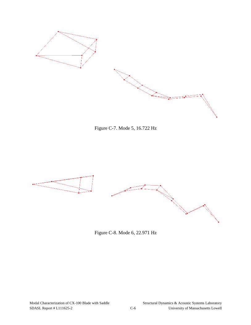
5 16.722 0.68% Flap
6 22.971 1.95% Flap
7 25.258 3.44% Edge
8 33.764 0.61% Edge
The resulting mode shapes are shown in Appendix C.
All test set up and log sheets are included in Appendix D.
The measurement data is stored in universal file format as:
“NREL_CX100_With_Saddle_120111_Measurements.unv”
The geometry is stored as:
“CX_100_and_Fixture_Geometry.unv”
The mode shapes are stored as:
“NREL_CX100_Saddle_Shapes.unv”

Modal Characterization of CX-100 Blade with Saddle Structural Dynamics & Acoustic Systems Laboratory
SDASL Report # L111625-2 A-1 University of Massachusetts Lowell
Appendix A
Equipment List

Modal Characterization of CX-100 Blade with Saddle Structural Dynamics & Acoustic Systems Laboratory
SDASL Report # L111625-2 A-2 University of Massachusetts Lowell
Table A-1. Equipment List Name Model Serial No. Sensitivity
Small Modal Impact Sledgehammer 086C20 12021 1 mV/lbf
Accelerometer Pt. 13+X 336C 11342 1.00800 V/g
Accelerometer Pt. 13-Y 336C 11328 1.02200 V/g
Accelerometer Pt. 29+X 336C 14968 1.01500 V/g
Accelerometer Pt. 29-Y 336C 13473 1.02400 V/g
Accelerometer Pt. 32+X 336C 12313 1.02300 V/g
Accelerometer Pt. 32-Y 336C31 8975 0.97240 V/g
Accelerometer Pt. 46+X 336C31 8867 1.00080 V/g
Accelerometer Pt. 46-Y 336C31 8870 1.00600 V/g
Accelerometer Pt. 48+X 336C 14970 0.98000 V/g
Accelerometer Pt. 48-Y 336C 15522 1.01300 V/g
Accelerometer Pt. 62+X 336C31 8873 0.99430 V/g
Accelerometer Pt. 62-Y 336C 11337 1.05400 V/g
Accelerometer Pt. 64+X 336C 11320 1.02600 V/g
Accelerometer Pt. 64-Y 336C 11326 1.01400 V/g
Accelerometer Pt. 74+X 336C 11335 1.04800 V/g
Accelerometer Pt. 74-Y 336C 11336 1.01800 V/g
Accelerometer Pt. 75+X 336C 13477 1.00300 V/g
Accelerometer Pt. 75-Y 336C 11324 1.02500 V/g
Accelerometer Pt. 82+X 336C 13472 1.00900 V/g
Accelerometer Pt. 82-Y 336C 11329 1.01500 V/g
Accelerometer Pt. 83+X 336C 15518 1.01000 V/g
Accelerometer Pt. 83-Y 336C31 8857 1.00910 V/g
Accelerometer Pt. 90+X 336C 15520 1.10000 V/g
Accelerometer Pt. 90-Y 336C31 8865 1.01162 V/g
Accelerometer Pt. 91+X 336C 11330 1.00800 V/g
Accelerometer Pt. 91-Y 336C 15519 1.02000 V/g
Accelerometer Pt. 96+X 336C 11334 1.03100 V/g
Accelerometer Pt. 96-Y 336C 11333 1.02100 V/g
Accelerometer Pt. 101+X 336C 13476 1.00200 V/g
Accelerometer Pt. 101+Z 336C 13480 1.01300 V/g
Accelerometer Pt. 102-X 336C 11332 1.01900 V/g
Accelerometer Pt. 102+Z 336C 15521 0.99000 V/g
Accelerometer Pt. 103+X 336C 11321 1.02100 V/g
Accelerometer Pt. 103+Z 336C 14978 1.02000 V/g
Accelerometer Pt. 104-X 336C 11322 1.01000 V/g
Accelerometer Pt. 104+Z 336C 11327 1.00400 V/g
Accelerometer Pt. 105+X 336C 14977 1.02200 V/g
Accelerometer Pt. 105-Y 336C 13474 0.99400 V/g
Accelerometer Pt. 107-X 336C 11339 1.03300 V/g
Accelerometer Pt. 107-Y 336C 14979 0.94000 V/g

Modal Characterization of CX-100 Blade with Saddle Structural Dynamics & Acoustic Systems Laboratory
SDASL Report # L111625-2 B-1 University of Massachusetts Lowell
Appendix B
Test Photos

Modal Characterization of CX-100 Blade with Saddle Structural Dynamics & Acoustic Systems Laboratory
SDASL Report # L111625-2 B-2 University of Massachusetts Lowell
Figure B-1. Blade Mounted to Fixture.

Modal Characterization of CX-100 Blade with Saddle Structural Dynamics & Acoustic Systems Laboratory
SDASL Report # L111625-2 B-3 University of Massachusetts Lowell
Figure B-2. General View of Accelerometers on Blade

Modal Characterization of CX-100 Blade with Saddle Structural Dynamics & Acoustic Systems Laboratory
SDASL Report # L111625-2 B-4 University of Massachusetts Lowell
Figure B-3. Blade with Saddle.

Modal Characterization of CX-100 Blade with Saddle Structural Dynamics & Acoustic Systems Laboratory
SDASL Report # L111625-2 B-5 University of Massachusetts Lowell
Figure B-4. Close-up of Saddle

Modal Characterization of CX-100 Blade with Saddle Structural Dynamics & Acoustic Systems Laboratory
SDASL Report # L111625-2 B-6 University of Massachusetts Lowell
Figure B-5. Back of Fixture.

Modal Characterization of CX-100 Blade with Saddle Structural Dynamics & Acoustic Systems Laboratory
SDASL Report # L111625-2 B-7 University of Massachusetts Lowell
Figure B-6. Impacting in Flapwise Direction.

Modal Characterization of CX-100 Blade with Saddle Structural Dynamics & Acoustic Systems Laboratory
SDASL Report # L111625-2 B-8 University of Massachusetts Lowell
Figure B-7. Impacting in Edgewise Direction.

Modal Characterization of CX-100 Blade with Saddle Structural Dynamics & Acoustic Systems Laboratory
SDASL Report # L111625-2 B-9 University of Massachusetts Lowell
Figure B-8. Accelerometer on Mounting Block: Point 90, Top View

Modal Characterization of CX-100 Blade with Saddle Structural Dynamics & Acoustic Systems Laboratory
SDASL Report # L111625-2 B-10 University of Massachusetts Lowell
Figure B-9. Accelerometer on Mounting Block: Point 90, Side View

Modal Characterization of CX-100 Blade with Saddle Structural Dynamics & Acoustic Systems Laboratory
SDASL Report # L111625-2 B-11 University of Massachusetts Lowell
Figure B-10. Accelerometer Level with Glue.

Modal Characterization of CX-100 Blade with Saddle Structural Dynamics & Acoustic Systems Laboratory
SDASL Report # L111625-2 B-12 University of Massachusetts Lowell
Figure B-11. Accelerometer on Fixture, Point 1.

Modal Characterization of CX-100 Blade with Saddle Structural Dynamics & Acoustic Systems Laboratory
SDASL Report # L111625-2 C-1 University of Massachusetts Lowell
Appendix C
Sample FRFs and Mode Shapes

Modal Characterization of CX-100 Blade with Saddle Structural Dynamics & Acoustic Systems Laboratory
SDASL Report # L111625-2 C-2 University of Massachusetts Lowell
Figure C-1. Drive Point FRF and Coherence at 90X (Edgewise)
0.00 50.00Linear
Hz
-60.00
0.00dB
g/lb
f
0.00 50.00Linear
Hz
0.00 50.00Hz
0.06
1.00
Am
plit
ude
/

Modal Characterization of CX-100 Blade with Saddle Structural Dynamics & Acoustic Systems Laboratory
SDASL Report # L111625-2 C-3 University of Massachusetts Lowell
Figure C-2. Drive Point FRF and Coherence at 90Y (Flapwise)
0.00 50.00Linear
Hz
-90.00
0.00
dB
g/lb
f
0.00 50.00Linear
Hz
0.00 50.00Hz
0.00
1.00
Am
plit
ude
/

Modal Characterization of CX-100 Blade with Saddle Structural Dynamics & Acoustic Systems Laboratory
SDASL Report # L111625-2 C-4 University of Massachusetts Lowell
Figure C-3. Mode 1, 1.868 Hz
Figure C-4. Mode 2, 2.728 Hz

Modal Characterization of CX-100 Blade with Saddle Structural Dynamics & Acoustic Systems Laboratory
SDASL Report # L111625-2 C-5 University of Massachusetts Lowell
Figure C-5. Mode 3, 8.886 Hz
Figure C-6. Mode 4, 9.671 Hz
Modal Characterization of CX-100 Blade with Saddle Structural Dynamics & Acoustic Systems Laboratory
SDASL Report # L111625-2 C-6 University of Massachusetts Lowell
Figure C-7. Mode 5, 16.722 Hz
Figure C-8. Mode 6, 22.971 Hz

Modal Characterization of CX-100 Blade with Saddle Structural Dynamics & Acoustic Systems Laboratory
SDASL Report # L111625-2 C-7 University of Massachusetts Lowell
Figure C-9. Mode 7, 25.258 Hz
Figure C-10. Mode 8, 33.764 Hz

Modal Characterization of CX-100 Blade with Saddle Structural Dynamics & Acoustic Systems Laboratory
SDASL Report # L111625-2 D-1 University of Massachusetts Lowell
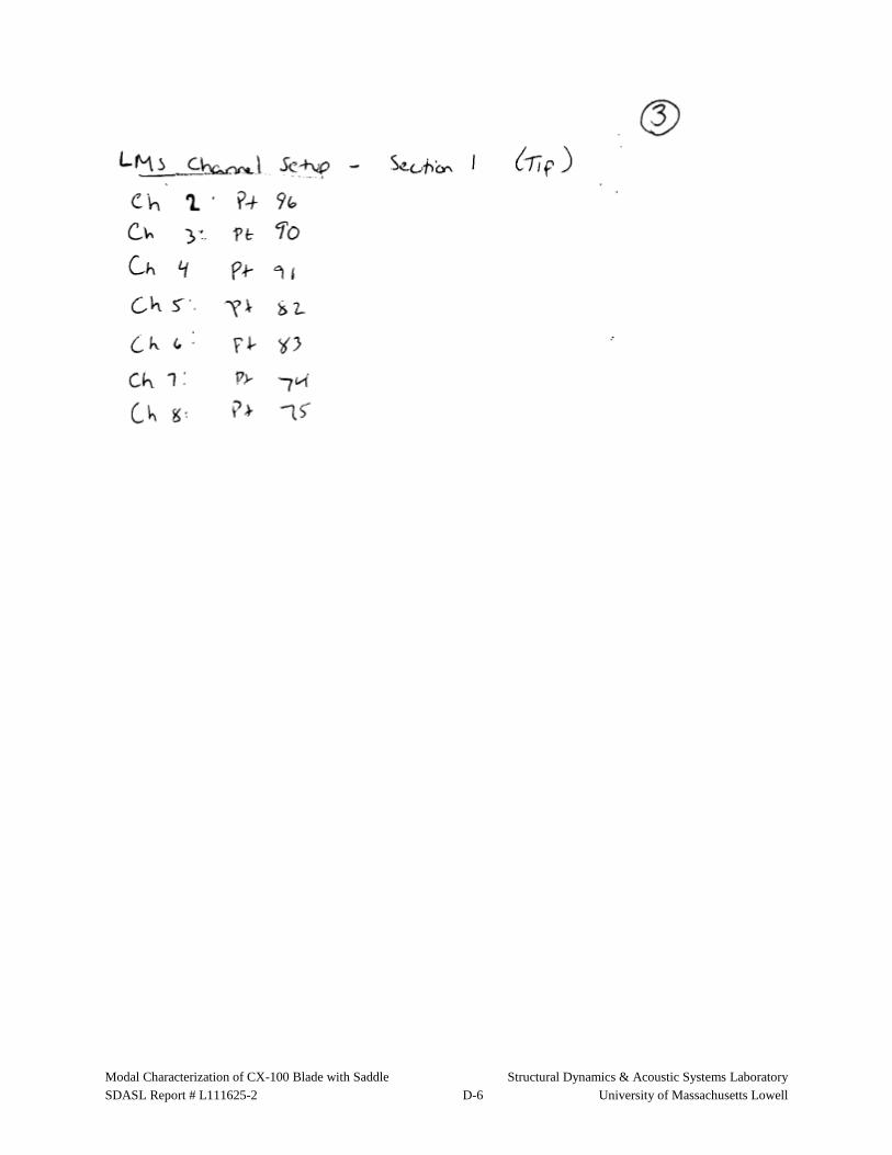
Appendix D
Test Sheets

Modal Characterization of CX-100 Blade with Saddle Structural Dynamics & Acoustic Systems Laboratory
SDASL Report # L111625-2 D-2 University of Massachusetts Lowell

Modal Characterization of CX-100 Blade with Saddle Structural Dynamics & Acoustic Systems Laboratory
SDASL Report # L111625-2 D-3 University of Massachusetts Lowell

Modal Characterization of CX-100 Blade with Saddle Structural Dynamics & Acoustic Systems Laboratory
SDASL Report # L111625-2 D-4 University of Massachusetts Lowell

Modal Characterization of CX-100 Blade with Saddle Structural Dynamics & Acoustic Systems Laboratory
SDASL Report # L111625-2 D-5 University of Massachusetts Lowell
Modal Characterization of CX-100 Blade with Saddle Structural Dynamics & Acoustic Systems Laboratory
SDASL Report # L111625-2 D-6 University of Massachusetts Lowell

Modal Characterization of CX-100 Blade with Saddle Structural Dynamics & Acoustic Systems Laboratory
SDASL Report # L111625-2 D-7 University of Massachusetts Lowell

Modal Characterization of CX-100 Blade with Saddle Structural Dynamics & Acoustic Systems Laboratory
SDASL Report # L111625-2 D-8 University of Massachusetts Lowell

Modal Characterization of CX-100 Blade with Saddle Structural Dynamics & Acoustic Systems Laboratory
SDASL Report # L111625-2 D-9 University of Massachusetts Lowell

Modal Characterization of CX-100 Blade with Saddle Structural Dynamics & Acoustic Systems Laboratory
SDASL Report # L111625-2 D-10 University of Massachusetts Lowell

Modal Characterization of CX-100 Blade with Saddle Structural Dynamics & Acoustic Systems Laboratory
SDASL Report # L111625-2 D-11 University of Massachusetts Lowell

Modal Characterization of CX-100 Blade with Saddle Structural Dynamics & Acoustic Systems Laboratory
SDASL Report # L111625-2 D-12 University of Massachusetts Lowell

Universal File Format Specification Structural Dynamics & Acoustic Systems Laboratory
SDASL Report # L111625-2 E-1 University of Massachusetts Lowell
Appendix E
Universal File Format Specifications
NOTE: While this appendix identifies the typical universal file format,
there is no guarantee that all vendors follow this format exactly.

Universal File Format Specification Structural Dynamics & Acoustic Systems Laboratory
SDASL Report # L111625-2 E-2 University of Massachusetts Lowell
Universal Dataset Number: 58
Name: Function at Nodal DOF
Status: Current
Owner: Test
Revision Date: 23-Apr-1993
-----------------------------------------------------------------------
Record 1: Format(80A1)
Field 1 - ID Line 1
NOTE
ID Line 1 is generally used for the function
description.
Record 2: Format(80A1)
Field 1 - ID Line 2
Record 3: Format(80A1)
Field 1 - ID Line 3
NOTE
ID Line 3 is generally used to identify when the
function was created. The date is in the form
DD-MMM-YY, and the time is in the form HH:MM:SS,
with a general Format(9A1,1X,8A1).
Record 4: Format(80A1)
Field 1 - ID Line 4
Record 5: Format(80A1)
Field 1 - ID Line 5
Record 6: Format(2(I5,I10),2(1X,10A1,I10,I4))
DOF Identification
Field 1 - Function Type
0 - General or Unknown
1 - Time Response
2 - Auto Spectrum
3 - Cross Spectrum
4 - Frequency Response Function
5 - Transmissibility
6 - Coherence
7 - Auto Correlation
8 - Cross Correlation
9 - Power Spectral Density (PSD)
10 - Energy Spectral Density (ESD)
11 - Probability Density Function
12 - Spectrum
13 - Cumulative Frequency Distribution
14 - Peaks Valley
15 - Stress/Cycles
16 - Strain/Cycles
17 - Orbit
18 - Mode Indicator Function
19 - Force Pattern
20 - Partial Power
21 - Partial Coherence
22 - Eigenvalue

Universal File Format Specification Structural Dynamics & Acoustic Systems Laboratory
SDASL Report # L111625-2 E-3 University of Massachusetts Lowell
23 - Eigenvector
24 - Shock Response Spectrum
25 - Finite Impulse Response Filter
26 - Multiple Coherence
27 - Order Function
Field 2 - Function Identification Number
Field 3 - Version Number, or sequence number
Field 4 - Load Case Identification Number
0 - Single Point Excitation
Field 5 - Response Entity Name ("NONE" if unused)
Field 6 - Response Node
Field 7 - Response Direction
0 - Scalar
1 - +X Translation 4 - +X
Rotation
-1 - -X Translation -4 - -X
Rotation
2 - +Y Translation 5 - +Y
Rotation
-2 - -Y Translation -5 - -Y
Rotation
3 - +Z Translation 6 - +Z
Rotation
-3 - -Z Translation -6 - -Z
Rotation
Field 8 - Reference Entity Name ("NONE" if unused)
Field 9 - Reference Node
Field 10 - Reference Direction (same as field 7)
NOTE
Fields 8, 9, and 10 are only relevant if field 4
is zero.
Record 7: Format(3I10,3E13.5)
Data Form
Field 1 - Ordinate Data Type
2 - real, single precision
4 - real, double precision
5 - complex, single precision
6 - complex, double precision
Field 2 - Number of data pairs for uneven abscissa
spacing, or number of data values for even
abscissa spacing
Field 3 - Abscissa Spacing
0 - uneven
1 - even (no abscissa values stored)
Field 4 - Abscissa minimum (0.0 if spacing uneven)
Field 5 - Abscissa increment (0.0 if spacing uneven)
Field 6 - Z-axis value (0.0 if unused)
Record 8: Format(I10,3I5,2(1X,20A1))
Abscissa Data Characteristics
Field 1 - Specific Data Type
0 - unknown
1 - general
2 - stress
3 - strain
5 - temperature
6 - heat flux
8 - displacement
9 - reaction force

Universal File Format Specification Structural Dynamics & Acoustic Systems Laboratory
SDASL Report # L111625-2 E-4 University of Massachusetts Lowell
11 - velocity
12 - acceleration
13 - excitation force
15 - pressure
16 - mass
17 - time
18 - frequency
19 - rpm
20 - order
Field 2 - Length units exponent
Field 3 - Force units exponent
Field 4 - Temperature units exponent
NOTE
Fields 2, 3 and 4 are relevant only if the
Specific Data Type is General, or in the case of
ordinates, the response/reference direction is a
scalar, or the functions are being used for
nonlinear connectors in System Dynamics Analysis.
See Addendum 'A' for the units exponent table.
Field 5 - Axis label ("NONE" if not used)
Field 6 - Axis units label ("NONE" if not used)
NOTE
If fields 5 and 6 are supplied, they take
precendence over program generated labels and
units.
Record 9: Format(I10,3I5,2(1X,20A1))
Ordinate (or ordinate numerator) Data
Characteristics
Record 10: Format(I10,3I5,2(1X,20A1))
Ordinate Denominator Data Characteristics
Record 11: Format(I10,3I5,2(1X,20A1))
Z-axis Data Characteristics
NOTE
Records 9, 10, and 11 are always included and
have fields the same as record 8. If records 10
and 11 are not used, set field 1 to zero.
Record 12:
Data Values
Ordinate Abscissa
Case Type Precision Spacing Format
-------------------------------------------------------------
1 real single even 6E13.5
2 real single uneven 6E13.5
3 complex single even 6E13.5
4 complex single uneven 6E13.5
5 real double even 4E20.12
6 real double uneven 2(E13.5,E20.12)
7 complex double even 4E20.12
8 complex double uneven E13.5,2E20.12
--------------------------------------------------------------

Universal File Format Specification Structural Dynamics & Acoustic Systems Laboratory
SDASL Report # L111625-2 E-5 University of Massachusetts Lowell
NOTE
See Addendum 'B' for typical FORTRAN READ/WRITE statements for each case.
General Notes:
1. ID lines may not be blank. If no information is required,
the word "NONE" must appear in columns 1 through 4.
2. ID line 1 appears on plots in Finite Element Modeling and is
used as the function description in System Dynamics Analysis.
3. Dataloaders use the following ID line conventions
ID Line 1 - Model Identification
ID Line 2 - Run Identification
ID Line 3 - Run Date and Time
ID Line 4 - Load Case Name
4. Coordinates codes from MODAL-PLUS and MODALX are decoded into
node and direction.
5. Entity names used in System Dynamics Analysis prior to I-DEAS
Level 5 have a 4 character maximum. Beginning with Level 5,
entity names will be ignored if this dataset is preceded by
dataset 259. If no dataset 259 precedes this dataset, then the
entity name will be assumed to exist in model bin number 1.
6. Record 10 is ignored by System Dynamics Analysis unless load
case = 0. Record 11 is always ignored by System Dynamics Analysis.
7. In record 6, if the response or reference names are "NONE"
and are not overridden by a dataset 259, but the correspond-
ing node is non-zero, System Dynamics Analysis adds the node
and direction to the function description if space is sufficie
8. ID line 1 appears on XY plots in Test Data Analysis along
with ID line 5 if it is defined. If defined, the axis units
labels also appear on the XY plot instead of the normal
labeling based on the data type of the function.
9. For functions used with nonlinear connectors in System
Dynamics Analysis, the following requirements must be
adhered to:
a) Record 6: For a displacement-dependent function, the
function type must be 0; for a frequency-dependent
function, it must be 4. In either case, the load case
identification number must be 0.
b) Record 8: For a displacement-dependent function, the
specific data type must be 8 and the length units
exponent must be 0 or 1; for a frequency-dependent
function, the specific data type must be 18 and the
length units exponent must be 0. In either case, the
other units exponents must be 0.
c) Record 9: The specific data type must be 13. The
temperature units exponent must be 0. For an ordinate
numerator of force, the length and force units
exponents must be 0 and 1, respectively. For an
ordinate numerator of moment, the length and force
units exponents must be 1 and 1, respectively.

Universal File Format Specification Structural Dynamics & Acoustic Systems Laboratory
SDASL Report # L111625-2 E-6 University of Massachusetts Lowell
d) Record 10: The specific data type must be 8 for
stiffness and hysteretic damping; it must be 11
for viscous damping. For an ordinate denominator of
translational displacement, the length units exponent
must be 1; for a rotational displacement, it must
be 0. The other units exponents must be 0.
e) Dataset 217 must precede each function in order to
define the function's usage (i.e. stiffness, viscous
damping, hysteretic damping).
Addendum A
In order to correctly perform units conversion, length, force, and
temperature exponents must be supplied for a specific data type of
General; that is, Record 8 Field 1 = 1. For example, if the function
has the physical dimensionality of Energy (Force * Length), then the
required exponents would be as follows:
Length = 1
Force = 1 Energy = L * F
Temperature = 0
Units exponents for the remaining specific data types should not be
supplied. The following exponents will automatically be used.
Table - Unit Exponents
-------------------------------------------------------
Specific Direction
---------------------------------------------
Data Translational Rotational
---------------------------------------------
Type Length Force Temp Length Force Temp
-------------------------------------------------------
0 0 0 0 0 0 0
1 (requires input to fields 2,3,4)
2 -2 1 0 -1 1 0
3 0 0 0 0 0 0
5 0 0 1 0 0 1
6 1 1 0 1 1 0
8 1 0 0 0 0 0
9 0 1 0 1 1 0
11 1 0 0 0 0 0
12 1 0 0 0 0 0
13 0 1 0 1 1 0
15 -2 1 0 -1 1 0
16 -1 1 0 1 1 0
17 0 0 0 0 0 0
18 0 0 0 0 0 0
19 0 0 0 0 0 0
--------------------------------------------------------
NOTE
Units exponents for scalar points are defined within
System Analysis prior to reading this dataset.
Addendum B
There are 8 distinct combinations of parameters which affect the
details of READ/WRITE operations. The parameters involved are

Universal File Format Specification Structural Dynamics & Acoustic Systems Laboratory
SDASL Report # L111625-2 E-7 University of Massachusetts Lowell
Ordinate Data Type, Ordinate Data Precision, and Abscissa Spacing.
Each combination is documented in the examples below. In all cases,
the number of data values (for even abscissa spacing) or data pairs
(for uneven abscissa spacing) is NVAL. The abcissa is always real
single precision. Complex double precision is handled by two real
double precision variables (real part followed by imaginary part)
because most systems do not directly support complex double precision.
CASE 1
REAL
SINGLE PRECISION
EVEN SPACING
Order of data in file Y1 Y2 Y3 Y4 Y5 Y6
Y7 Y8 Y9 Y10 Y11 Y12
.
.
.
Input
REAL Y(6)
.
.
.
NPRO=0
10 READ(LUN,1000,ERR= ,END= )(Y(I),I=1,6)
1000 FORMAT(6E13.5)
NPRO=NPRO+6
.
. code to process these six values
.
IF(NPRO.LT.NVAL)GO TO 10
.
. continued processing
.
Output
REAL Y(6)
.
.
.
NPRO=0
10 CONTINUE
.
. code to set up these six values
.
WRITE(LUN,1000,ERR= )(Y(I),I=1,6)
1000 FORMAT(6E13.5)
NPRO=NPRO+6
IF(NPRO.LT.NVAL)GO TO 10
.
. continued processing
.
CASE 2
REAL
SINGLE PRECISION
UNEVEN SPACING

Universal File Format Specification Structural Dynamics & Acoustic Systems Laboratory
SDASL Report # L111625-2 E-8 University of Massachusetts Lowell
Order of data in file X1 Y1 X2 Y2 X3 Y3
X4 Y4 X5 Y5 X6 Y6
.
.
.
Input
REAL X(3),Y(3)
.
.
.
NPRO=0
10 READ(LUN,1000,ERR= ,END= )(X(I),Y(I),I=1,3)
1000 FORMAT(6E13.5)
NPRO=NPRO+3
.
. code to process these three values
.
IF(NPRO.LT.NVAL)GO TO 10
.
. continued processing
.
Output
REAL X(3),Y(3)
.
.
.
NPRO=0
10 CONTINUE
.
. code to set up these three values
.
WRITE(LUN,1000,ERR= )(X(I),Y(I),I=1,3)
1000 FORMAT(6E13.5)
NPRO=NPRO+3
IF(NPRO.LT.NVAL)GO TO 10
.
. continued processing
.
CASE 3
COMPLEX
SINGLE PRECISION
EVEN SPACING
Order of data in file RY1 IY1 RY2 IY2 RY3 IY3
RY4 IY4 RY5 IY5 RY6 IY6
.
.
.
Input
COMPLEX Y(3)
.
.
.
NPRO=0

Universal File Format Specification Structural Dynamics & Acoustic Systems Laboratory
SDASL Report # L111625-2 E-9 University of Massachusetts Lowell
10 READ(LUN,1000,ERR= ,END= )(Y(I),I=1,3)
1000 FORMAT(6E13.5)
NPRO=NPRO+3
.
. code to process these six values
.
IF(NPRO.LT.NVAL)GO TO 10
.
. continued processing
.
Output
COMPLEX Y(3)
.
.
.
NPRO=0
10 CONTINUE
.
. code to set up these three values
.
WRITE(LUN,1000,ERR= )(Y(I),I=1,3)
1000 FORMAT(6E13.5)
NPRO=NPRO+3
IF(NPRO.LT.NVAL)GO TO 10
.
. continued processing
.
CASE 4
COMPLEX
SINGLE PRECISION
UNEVEN SPACING
Order of data in file X1 RY1 IY1 X2 RY2 IY2
X3 RY3 IY3 X4 RY4 IY4
.
.
.
Input
REAL X(2)
COMPLEX Y(2)
.
.
.
NPRO=0
10 READ(LUN,1000,ERR= ,END= )(X(I),Y(I),I=1,2)
1000 FORMAT(6E13.5)
NPRO=NPRO+2
.
. code to process these two values
.
IF(NPRO.LT.NVAL)GO TO 10
.
. continued processing
.

Universal File Format Specification Structural Dynamics & Acoustic Systems Laboratory
SDASL Report # L111625-2 E-10 University of Massachusetts Lowell
Output
REAL X(2)
COMPLEX Y(2)
.
.
.
NPRO=0
10 CONTINUE
.
. code to set up these two values
.
WRITE(LUN,1000,ERR= )(X(I),Y(I),I=1,2)
1000 FORMAT(6E13.5)
NPRO=NPRO+2
IF(NPRO.LT.NVAL)GO TO 10
.
. continued processing
.
CASE 5
REAL
DOUBLE PRECISION
EVEN SPACING
Order of data in file Y1 Y2 Y3 Y4
Y5 Y6 Y7 Y8
.
.
.
Input
DOUBLE PRECISION Y(4)
.
.
.
NPRO=0
10 READ(LUN,1000,ERR= ,END= )(Y(I),I=1,4)
1000 FORMAT(4E20.12)
NPRO=NPRO+4
.
. code to process these four values
.
IF(NPRO.LT.NVAL)GO TO 10
.
. continued processing
.
Output
DOUBLE PRECISION Y(4)
.
.
.
NPRO=0
10 CONTINUE
.
. code to set up these four values
.
WRITE(LUN,1000,ERR= )(Y(I),I=1,4)
1000 FORMAT(4E20.12)

Universal File Format Specification Structural Dynamics & Acoustic Systems Laboratory
SDASL Report # L111625-2 E-11 University of Massachusetts Lowell
NPRO=NPRO+4
IF(NPRO.LT.NVAL)GO TO 10
.
. continued processing
.
CASE 6
REAL
DOUBLE PRECISION
UNEVEN SPACING
Order of data in file X1 Y1 X2 Y2
X3 Y3 X4 Y4
.
.
.
Input
REAL X(2)
DOUBLE PRECISION Y(2)
.
.
.
NPRO=0
10 READ(LUN,1000,ERR= ,END= )(X(I),Y(I),I=1,2)
1000 FORMAT(2(E13.5,E20.12))
NPRO=NPRO+2
.
. code to process these two values
.
IF(NPRO.LT.NVAL)GO TO 10
.
. continued processing
.
Output
REAL X(2)
DOUBLE PRECISION Y(2)
.
.
.
NPRO=0
10 CONTINUE
.
. code to set up these two values
.
WRITE(LUN,1000,ERR= )(X(I),Y(I),I=1,2)
1000 FORMAT(2(E13.5,E20.12))
NPRO=NPRO+2
IF(NPRO.LT.NVAL)GO TO 10
.
. continued processing
.
CASE 7
COMPLEX
DOUBLE PRECISION
EVEN SPACING
Order of data in file RY1 IY1 RY2 IY2

Universal File Format Specification Structural Dynamics & Acoustic Systems Laboratory
SDASL Report # L111625-2 E-12 University of Massachusetts Lowell
RY3 IY3 RY4 IY4
.
.
.
Input
DOUBLE PRECISION Y(2,2)
.
.
.
NPRO=0
10 READ(LUN,1000,ERR= ,END= )((Y(I,J),I=1,2),J=1,2)
1000 FORMAT(4E20.12)
NPRO=NPRO+2
.
. code to process these two values
.
IF(NPRO.LT.NVAL)GO TO 10
.
. continued processing
.
Output
DOUBLE PRECISION Y(2,2)
.
.
.
NPRO=0
10 CONTINUE
.
. code to set up these two values
.
WRITE(LUN,1000,ERR= )((Y(I,J),I=1,2),J=1,2)
1000 FORMAT(4E20.12)
NPRO=NPRO+2
IF(NPRO.LT.NVAL)GO TO 10
.
. continued processing
.
CASE 8
COMPLEX
DOUBLE PRECISION
UNEVEN SPACING
Order of data in file X1 RY1 IY1
X2 RY2 IY2
.
.
.
Input
REAL X
DOUBLE PRECISION Y(2)
.
.
.
NPRO=0
10 READ(LUN,1000,ERR= ,END= )(X,Y(I),I=1,2)
1000 FORMAT(E13.5,2E20.12)
NPRO=NPRO+1

Universal File Format Specification Structural Dynamics & Acoustic Systems Laboratory
SDASL Report # L111625-2 E-13 University of Massachusetts Lowell
.
. code to process this value
.
IF(NPRO.LT.NVAL)GO TO 10
.
. continued processing
.
Output
REAL X
DOUBLE PRECISION Y(2)
.
.
.
NPRO=0
10 CONTINUE
.
. code to set up this value
.
WRITE(LUN,1000,ERR= )(X,Y(I),I=1,2)
1000 FORMAT(E13.5,2E20.12)
NPRO=NPRO+1
IF(NPRO.LT.NVAL)GO TO 10
.
. continued processing
.
-----------------------------------------------------------------------