IMPACT OF WATER LEVEL FLUCTUATIONS AND FISH ON MACROINVERTEBRATE COMMUNITY AND PERIPHYTON GROWTH IN

SHALLOW LAKES - A MESOCOSM APPROACH

A THESIS SUBMITTED TO THE GRADUATE SCHOOL OF NATURAL AND APPLIED SCIENCES

OF MIDDLE EAST TECHNICAL UNIVERSITY

BY

ECE SARAOĞLU

IN PARTIAL FULFILLMENT OF THE REQUIREMENTS FOR

THE DEGREE OF MASTER OF SCIENCE IN

BIOLOGY

FEBRUARY 2012

ii

Approval of the thesis:

IMPACT OF WATER LEVEL FLUCTUATIONS AND FISH ON MACROINVERTEBRATE COMMUNITY AND PERIPHYTON GROWTH IN

SHALLOW LAKES - A MESOCOSM APPROACH

submitted by ECE SARAOĞLU in partial fulfillment of the requirements for the degree of Master of Science in Biology Department, Middle East Technical University by,

Prof. Dr. Canan Özgen Dean, Graduate School of Natural and Applied Sciences Prof. Dr. Musa Doğan Head of Department, Biology Prof. Dr. Meryem Beklioğlu Yerli Supervisor, Biology Department, METU Prof. Dr. Erik Jeppesen Co-Supervisor, Biology Department, Aarhus University

Examining Committee Members: Prof. Dr. Ayşen Yılmaz Institute of Marine Sciences, METU Prof. Dr. Meryem Beklioğlu Yerli Biology Department, METU Assoc. Prof. Dr. Can Bilgin Biology Department, METU Assoc. Prof. Ayşegül Gözen Biology Department, METU Assist. Prof. Dr. Ayşegül Birand Biology Department, METU

Date: 10.02.2012

iii

I hereby declare that all information in this document has been obtained and presented in accordance with academic rules and ethical conduct. I also declare that, as required by these rules and conduct, I have fully cited and referenced all material and results that are not original to this work.

Name, Last Name : Ece Saraoğlu

Signature :

iv

ABSTRACT

IMPACT OF WATER LEVEL FLUCTUATIONS AND FISH ON

MACROINVERTEBRATE COMMUNITY AND PERIPHYTON GROWTH IN

SHALLOW LAKES - A MESOCOSM APPROACH

Saraoğlu, Ece

M.S., Department of Biology

Supervisor: Prof. Dr. Meryem Beklioğlu Yerli

Co-Supervisor: Prof. Dr. Erik Jeppesen

February 2012, 68 pages

A mesocosm experiment was conducted in Lake Eymir between June –

September 2009 in order to elucidate the effects of water level changes and

fish predation on periphyton growth and macroinvertebrates in semi-arid

shallow lakes.

Twenty four cylindrical enclosures, each with 1.2 m diameter, open to lake

bottom and atmosphere, were placed at three different depths, i.e. 0.8 m (low

water level, LW), 1.6 m (high water level, HW) and 2.3 m (however, data

regarding the enclosures at 2.3 m were excluded in this study due to

complications after fifth sampling) to simulate water level fluctuations. At

each water level, four replicates were stocked with omnivorous–

planktivorous fish (Tinca tinca and Alburnus escherichii) and the other four

v

replicates were left fishless to observe the effect of fish predation. Ten shoots

of submerged macrophytes (Potamogeton pectinatus) were planted and six

polyethylene strips were hung in the water column in each enclosure to

monitor macrophyte and periphyton growth.

The mesocosms were sampled for physical, chemical and biological

parameters weekly in the first month and fortnightly thereafter. Benthic

macroinvertebrate samples were taken before the start, in the middle and at

the end of the experiment with Kajak corer. Macrophytes were harvested

after the last sampling for determination of dry weight, epiphyton, and the

associated macroinvertebrates. All macroinvertebrate samples were sieved

through 212 μm mesh size before identification and counting.

Over the course of the experiment, an average of 0.46 ± 0.03 m water level

decrease in the mesocosms triggered submerged macrophyte growth in all

LW enclosures, overriding the negative effects of fish predation. The results

indicate that while fish predation pressure had negative influences on

macroinvertebrate communities in terms of both abundance and richness,

structural complexity created by dense vegetation in the LW mesocosms

weakened the top-down effect of fish on macroinvertebrates by acting as a

refuge in this semi-arid shallow lake.

Keywords: Macroinvertebrate, Periphyton, Water Level, Fish Predation,

Mesocosm

vi

ÖZ

SIĞ GÖLLERDE SU SEVİYESİ DEĞİŞİMİ VE BALIK BESLENMESİNİN

MAKROOMURGASIZ TOPLULUKLARI VE PERİFİTON BÜYÜMESİ ÜZERİNDEKİ

ETKİLERİ - MEZOKOZM YAKLAŞIMI

Saraoğlu, Ece

Yüksek Lisans, Biyoloji Bölümü

Tez Yöneticisi: Prof. Dr. Meryem Beklioğlu Yerli

Ortak Tez Yöneticisi: Prof. Dr. Erik Jeppesen

Şubat 2012, 68 sayfa

Su seviyesi değişimi ve balık beslenmesinin yarı-kurak sığ göllerde perifiton

büyümesi ve makroomurgasızlar üzerindeki etkilerini belirlemek amacıyla,

Haziran – Eylül 2009 tarihleri arasında Eymir Gölü’nde bir mezokozm deneyi

gerçekleştirilmiştir.

Her biri 1,2 m çapında, göl tabanına ve atmosfere açık olan silindir şeklindeki

yirmi dört adet deney düzeneği 0,8 m (düşük su seviyesi, LW), 1,6 m (yüksek

su seviyesi, HW) ve 2,3 m olmak üzere su seviyesi değişimini temsil eden üç

farklı derinliğe yerleştirilmiştir (ancak beşinci örneklemeden sonra

karşılaşılan sorun nedeniyle 2,3 m’deki düzeneklere ait veriler bu çalışmada

kullanılmamıştır). Balık beslenmesinin etkisini gözlemlemek amacıyla, her bir

su seviyesinde düzeneklerin dördüne omnivor-planktivor balıklar (Tinca

vii

tinca ve Alburnus escherichii) eklenmiş, kalan dört düzenek ise balıksız olarak

bırakılmıştır. Suiçi bitkisi ve perifiton büyümesini izlemek amacıyla tüm

düzeneklerin içine onar adet suiçi bitkisi (Potamogeton pectinatus) filizi

ekilmiş ve altışar adet polietilen şerit yerleştirilmiştir.

Fiziksel, kimyasal ve biyolojik parametreler ilk ay haftalık olarak, deneyin geri

kalanında ise iki haftada bir örneklenmiştir. Bentik makroomurgasız

örnekleri deneyin başında, ortasında ve sonunda Kajak tipi karotiyer ile

alınmıştır. Bitki kuru ağırlığı ve epifit miktarının belirlenmesi amacıyla suiçi

bitkileri son örneklemeden sonra toplanmış ve üzerindeki

makroomurgasızlar örneklenmiştir. Taksonomik sınıflandırma ve sayım için

tüm makroomurgasız örnekleri 212 μm’lik elekten geçirilmiştir.

Deney süresince mezokozmlardaki ortalama 0,46 ± 0,03 m’lik su seviyesi

düşüşü balık beslenmesinin olumsuz etkilerini telafi ederek, düşük su

seviyesindeki (LW) tüm düzeneklerde suiçi bitkilerinin büyümesini

sağlamıştır. Elde edilen sonuçlar, yarı-kurak sığ göllerde balık avlanma

baskısının makroomurgasız toplulukları üzerinde hem yoğunluk hem de

çeşitlilik açısından olumsuz etkileri olurken; LW düzeneklerinde su seviyesi

düşüşüyle desteklenen yoğun bitki gelişiminin sığınak rolü üstlenerek,

balıkların makroomurgasızlar üzerindeki yukarıdan aşağıya kontrolünü

zayıflattığını göstermektedir.

Anahtar Kelimeler: Makroomurgasız, Perifiton, Su Seviyesi, Balık Beslenmesi,

Mezokozm

viii

To my dear friends Seza Bürkan & Utku

ix

ACKNOWLEDGEMENTS

I am grateful to my supervisor Prof. Dr. Meryem Beklioğlu and my co-

supervisor Prof. Dr. Erik Jeppesen for their valuable guidance, inspiration and

support throughout my study.

I am also indebted to:

Current and former members of METU Limnology Laboratory (Arda Özen,

Ayşe İdil Çakıroğlu, Betül Acar, Eti Levi, Gizem Bezirci, Korhan Özkan, Merve

Tepe, Nihan Yazgan Tavşanoğlu, Nur Filiz, Şeyda Erdoğan, Tuba Bucak) for

their friendship and generous help with the field and laboratory work,

METU Subaqua Society divers (Bahattin Dinçel, Durmuş Yarımpabuç, Emrah

Cantekin who also aided with macroinvertebrate sorting as a second pair of

eyes, Hande Ceylan, Necati Çelik, Tolga Kanık, Volkan Ertürk, and in particular

to Esra Demirkol) for their effort in the establishment of the experimental

setup,

All the people who willingly helped during the construction phase of the

mesocosm setup and sampling (Çiğdem Cihangir, Erkan Aşık, Koray Yurtışık,

Mert Elverici, Nergis İrem Ertan, Oğuz Akçelik, Osman Karacan, Soner Oruç

and METU staff), Metehan Demirelli for the fish used in the experiment, and

METU Rowing Team and Lake Eymir staff for logistic support,

National Environmental Research Institute of Denmark (NERI) for counting

me as a member of the team, especially Thomas Boll Kristensen, Dr. Peter

Wiberg-Larsen and Johnny Nielsen for their help in macroinvertebrate

identification, and Anne Mette Poulsen and Carolina Trochine for their

comments on earlier drafts of this thesis.

x

A very special thanks goes to Tuba Bucak, the fellowship of the mesocosm, with

whom every occasion in the field became great fun, and countless hours of

laboratory work was bearable. Some people think it is not a big deal to write a

Master’s thesis. I agree with that, apart from the fact that our study required

extensive effort in the field and laboratory. So when this part was over (which

literally took months), writing the thesis was really not a big deal. Because

there you were, Tuba… not least when we broke down in tears after seeing

those dead carps in our precious mesocosms!

Lastly, I would like to express my eternal gratitude to my family, especially

my parents, for their patience, understanding and trust in me.

This project was funded by Middle East Technical University Scientific

Research Projects Coordinatorship (project number: BAP-07-02-2009-00-01).

xi

TABLE OF CONTENTS

ABSTRACT................................................................................................................................................... iv

ÖZ .................................................................................................................................................................... vi

ACKNOWLEDGEMENTS ........................................................................................................................ ix

TABLE OF CONTENTS ............................................................................................................................ xi

LIST OF TABLES .................................................................................................................................... xiii

LIST OF FIGURES ..................................................................................................................................... xv

LIST OF ABBREVIATIONS ................................................................................................................ xviii

CHAPTERS

1. INTRODUCTION .................................................................................................................................... 1

1.1 Shallow Lakes at a Glance .................................................................................... 1

1.2 Climate Change Effects on the Mediterranean Shallow Lakes ............. 4

1.3 Macroinvertebrates in Shallow Lake Ecosystems ..................................... 6

1.3.1 Water Level Fluctuations ................................................................................. 7

1.3.2 Fish Predation ................................................................................................... 10

1.4 Scope of the Study ................................................................................................ 11

2. MATERIALS & METHODS .............................................................................................................. 13

2.1 Study Site .................................................................................................................. 13

2.2 Experimental Setup: Mesocosms .................................................................. 16

2.3 Sampling and Processing ................................................................................... 22

xii

2.4 Laboratory Analysis ............................................................................................. 26

2.5 Statistical Analysis ................................................................................................ 28

3. RESULTS ............................................................................................................................................... 30

3.1 Physico-chemical Parameters ......................................................................... 30

3.2 Macrophytes, Epiphyton and Periphyton .................................................. 32

3.3 Macroinvertebrate Assemblages ................................................................... 36

3.3.1 Benthic Macroinvertebrates ....................................................................... 40

3.3.2 Macrophyte-associated Macroinvertebrates ....................................... 46

4. DISCUSSION & CONCLUSION ....................................................................................................... 49

4.1 Discussion ................................................................................................................ 49

4.1.1 Epiphyton and Periphyton ........................................................................... 50

4.1.2 Macroinvertebrates ........................................................................................ 52

4.2 Conclusion ................................................................................................................ 56

REFERENCES ........................................................................................................................................... 58

APPENDIX ................................................................................................................................................. 67

xiii

LIST OF TABLES

Table 1: Morphometric and hydrological characteristics of Lake Eymir

(Beklioglu et al., 2003; Özen et al., 2010) ........................................................................ 14

Table 2: Sampling dates ........................................................................................................... 22

Table 3: Macroinvertebrate sampling dates ................................................................... 25

Table 4: One-way ANOVA results showing the influence of water level on the

initial conditions of the parameters measured in time series and the

parameters sampled once (denoted by asterisks) in the mesocosms (ns

denotes a non-significant difference with p > 0.05.) (Bucak, 2011) .................... 31

Table 5: Average values [(mean ± standart error (SE)] of some physico-

chemical and biological parameters measured in the mesocosms and the

results of RM two-way ANOVA (only for macrophyte DW and epiphyton chl-a,

which did not have time series data, p values are results of two-way ANOVA)

(WL and F denote water level and fish, respectively. ns denotes a non-

significant difference with p > 0.05.) (Bucak, 2011) ................................................... 33

Table 6: Abundance (mean ± SD per sample) of benthic macroinvertebrates in

all treatments at the initial sampling (Dominant taxa are highlighted by

asterisks.) ....................................................................................................................................... 38

Table 7: Abundance (mean ± SD per sample) of benthic macroinvertebrates in

all treatments at the middle sampling (Dominant taxa are highlighted by

asterisks.) ....................................................................................................................................... 39

xiv

Table 8: Abundance (mean ± SD per sample) of benthic macroinvertebrates in

all treatments at the final sampling (Dominant taxa are highlighted by

asterisks.) ....................................................................................................................................... 39

Table 9: Abundance (mean ± SD per sample) of macrophyte-associated

macroinvertebrates in all treatments at the end of the experiment (Dominant

taxa are highlighted by asterisks.) ...................................................................................... 40

Table 10: One-way ANOVA results showing the influence of water level on the

initial sampling of benthic invertebrates (ns denotes a non-significant

difference with p>0.05.) .......................................................................................................... 40

Table 11: Two-way ANOVA results showing the influence of water level, fish

and their interaction on the middle sampling of benthic macroinvertebrates

(ns denotes a non-significant difference with p > 0.05.) ........................................... 44

Table 12: Two-way ANOVA results showing the influence of water level, fish

and their interaction on the final sampling of benthic macroinvertebrates (ns

denotes a non-significant difference with p > 0.05.) ................................................... 46

Table 13: Two-way ANOVA results showing the influence of water level, fish

and their interaction on the macrophyte-associated macroinvertebrates (ns

denotes a non-significant difference with p > 0.05.) ................................................... 47

xv

LIST OF FIGURES

Figure 1: Inflows and outflows of the study site, Lake Eymir, and its upstream

lake, Lake Mogan, and the location of the lakes on the map of Turkey (taken

from Özen et al., 2010) ............................................................................................................. 16

Figure 2: An illustration of the mesocosm setup (taken from Özkan, 2008) ... 18

Figure 3: Steps in mesocosm construction a) setting up cylindrical enclosures,

b) assembling aluminum frames, c) attaching PU foams to frames, d) placing

frames on site, e-f) installing and fixing mesocosms, g) planting macrophyte

shoots, h) covering mesocosms with netting ................................................................. 20

Figure 4: a) View from HW enclosures, b) Close-up view of a LW enclosure .. 21

Figure 5: Map of Lake Eymir and the locations of the mesocosms (Google

Earth, 2011) .................................................................................................................................. 21

Figure 6: a) Kajak core sampler, b) View from benthic macroinvertebrate

sampling ......................................................................................................................................... 25

Figure 7: Change in water levels of the mesocosms over the course of the

experiment .................................................................................................................................... 30

Figure 8: Ratio of Secchi disc depth to average depth of the mesocosms a)

change over the course of the experiment, b) comparison of all treatments at

the end of the experiment ...................................................................................................... 32

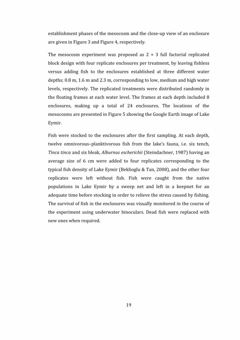
Figure 9: Macrophyte growth a) change in %PVI of the mesocosms over the

course of the experiment, b) macrophyte DW in all treatments at the end of

the experiment ............................................................................................................................ 34

xvi

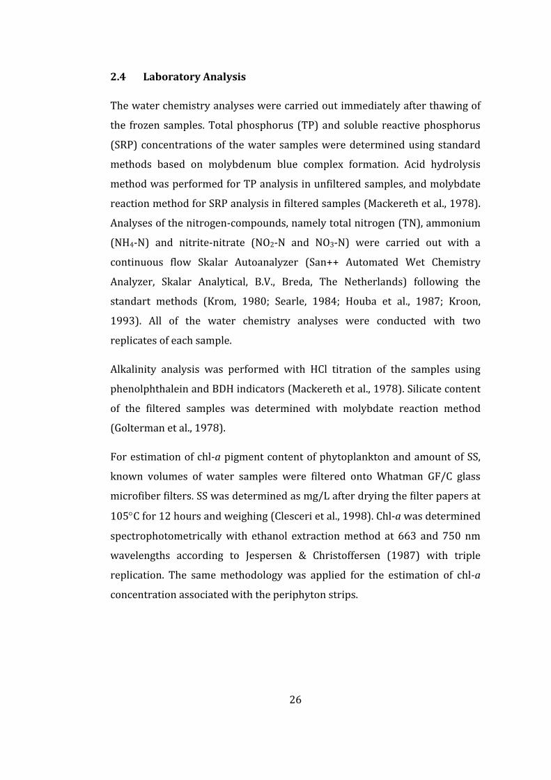
Figure 10: Epiphyton chl-a in all treatments at the end of the experiment ...... 34

Figure 11: Upper periphyton chl-a a) change over the course of the

experiment, b) comparison of all treatments in the last sampling ....................... 35

Figure 12: Bottom periphyton chl-a a) change over the course of the

experiment, b) comparison of all treatments in the last sampling ....................... 36

Figure 13: Change in mean (± SE) density in all treatments through the initial,

middle and final sampling of benthic macroinvertebrates ...................................... 41

Figure 14: Change in mean (± SE) taxa richness in all treatments through the

initial, middle and final sampling of benthic macroinvertebrates ........................ 41

Figure 15: Change in mean (± SE) predator density in all treatments through

the initial, middle and final sampling of benthic macroinvertebrates ................ 42

Figure 16: Change in mean (± SE) grazer-detritivore density in all treatments

through the initial, middle and final sampling of benthic macroinvertebrates

............................................................................................................................................................ 42

Figure 17: Change in mean (± SE) chironomid density through the initial,

middle and final sampling of benthic macroinvertebrates ...................................... 43

Figure 18: Change in mean (± SE) vulnerable density in all treatments through

the initial, middle and final sampling of benthic macroinvertebrates ................ 43

Figure 19: Density of benthic macroinvertebrates in all treatments in the

middle sampling ......................................................................................................................... 44

Figure 20: Taxa richness of benthic macroinvertebrates in all treatments in

the middle sampling .................................................................................................................. 45

Figure 21: Vulnerable density of benthic macroinvertebrates in all treatments

in the middle sampling............................................................................................................. 45

xvii

Figure 22: Predator density of benthic macroinvertebrates in all treatments in

the final sampling ....................................................................................................................... 46

Figure 23: Comparison of the parameters for macrophyte-associated

macroinvertebrates in all treatments a) total density, b) taxa richness (family

level), c) predator density, d) grazer-detritivore density, e) chironomid

density, f) vulnerable density ............................................................................................... 48

Figure 24: Conceptual response of macroinvertebrates to macrophyte growth

by decreasing water levels (Blue arrows indicate sampling dates.) .................... 56

xviii

LIST OF ABBREVIATIONS

ANOVA Analysis of variance

DW Dry weight

chl-a chlorophyll-a

F Fish

HW- High water level fishless

HW+ High water level with fish

LW- Low water level fishless

LW+ Low water level with fish

SD Standard deviation

SE Standard e

WL Water level

WLF Water level fluctuations

1

CHAPTER 1

INTRODUCTION

1.1 Shallow Lakes at a Glance

Freshwater lakes, though they comprise only a minor fraction (approximately

0.009 %) of the total available water in the Biosphere, are vital for terrestrial

life and fundamentally important hosts to rich biodiversity, thanks to their

littoral zone (Wetzel, 2001). Moreover, lentic ecosystems provide many

goods, materials and services to human beings, such as freshwater resources

for drinking, consumption and irrigation, fish stocks, recreation, and so forth.

However, misuse and overexploitation have led to deterioration of these

vulnerable ecosystems, especially after the industrial revolution.

Basins of large, deep lakes contain a considerable volume (almost 40%) of the

total available fresh water, and historically they have received much scientific

attention (Wetzel, 2001; Meerhoff, 2010). However, most of the millions of

lakes on earth (approximately 95%) are small (surface area <1 km2) and

relatively shallow (mean depth <10 m) (Wetzel, 2001). Over the last couple of

decades, the scientific interest in shallow lakes has accelerated worldwide

(Meerhoff, 2010).

Wetzel (2001) defined a shallow lake as a permanent standing body of water

that is sufficiently shallow to allow light penetration to the bottom sediments

adequate to potentially support photosynthesis of higher aquatic plants over

2

the entire basin. Shallow lakes usually do not experience thermal

stratification. They are characterized by a larger area for the interaction of

sediment-water interface and a higher rate of internal nutrients recycling.

Accordingly, they possess a larger littoral area, more abundant macrophytes

and usually a higher productivity per unit area of water than deep lakes

(Gasith & Hoyer, 1998; Moss, 1998; Wetzel, 2001). For this reason, shallow

lakes are crucial for the conservation of local and global biodiversity, though

their conservation value as a biodiversity resource is often overlooked.

Over a wide range of nutrient concentrations, shallow lakes can exist in two

alternative equilibria, i.e. macrophyte dominated clear water state and

phytoplankton dominated turbid water state. Shifts between these states may

have substantial impacts on ecosystems (Scheffer et al., 1993). Both states are

stable and triggered by several feedback mechanisms related to biological

interactions and physico-chemical processes. These mechanisms are needed

to be surpassed for a shift between the two states to occur (Blindow et al.,

1993; Scheffer et al., 1993; Scheffer, 1998).

When the nutrient concentrations are low, the lake is in a clear water state

characterized by dense macrophyte beds and low chlorophyll concentrations.

As compared to lakes without vegetation, vegetated lakes host richer

biodiversity, with abundance of invertebrates, fish and waterfowl (Scheffer et

al., 2006). Macrophytes provide refuge against predation by creating

heterogeneity, alter the nutrient dynamics of the system, prevent

resuspension of the sediment and enhance water clarity (Scheffer et al.,

1993). However, the lake may shift to an alternative equilibrium of

phytoplankton dominance and high chlorophyll concentrations. Nutrient

runoff caused by intensive agricultural practices and sewage disposal from

anthropogenic sources has lead to intensification of the eutrophication

phenomenon (Jeppesen, 1998), which is defined as the shift in the trophic

status of a water body towards a great increase in phytoplankton in response

3

to increased nitrogen (N) and phosphorous (P) loading. This eventuates in

deterioration of water clarity and loss of ecological and conservation values of

water bodies through elimination of predatory fish, submerged plants and

waterfowl (Scheffer et al., 1993).

Various abiotic factors and biotic processes act at different spatial and

temporal scales to shape the functioning and dynamics of shallow lakes. Some

of the most important abiotic factors are lake morphology, hydrology,

catchment and sediment characteristics, nutrient and light availability,

oxygen concentration, pH and temperature. Once these factors set the

background for the lake environment, biotic interactions such as predation

and competition for resources take the stage to determine the community

composition. Organisms affect each other either directly or through more

complex interactions (Brönmark & Hansson, 2002). This study focuses on two

of these variables, i.e. fish predation and changes in water level, and their

effects on macroinvertebrates will be discussed further in the following

sections.

Most studies about the functioning of shallow lakes have concentrated on the

northern temperate regions. However, recent studies have revealed that the

functioning of warmer shallow lakes differs from that of northern temperate

lakes. Shallow lakes in the subtropical regions and the semi-arid

Mediterranean basin exhibit contrasting characteristics such as prevalent

omnivory, weakened role of macrophytes as refuge, and higher abundance of

fish with smaller body size, especially through the plant beds (Meerhoff,

2006). The anticipated effects of global climate change on these lake

ecosystems accentuate the importance of scientific research on them (Coops

et al., 2003).

4

1.2 Climate Change Effects on the Mediterranean Shallow Lakes

The term "climate change" indicates a change of climate in addition to natural

climate variability observed over comparable time periods, and it is

attributed directly or indirectly to human activity that alters the composition

of the global atmosphere (UNFCCC, 2011).

As a result of burning greater amounts of fossil fuels after the industrial

revolution, deforestation and urbanization, the increasing greenhouse gas

concentrations in the atmosphere have intensified the greenhouse effect,

which has caused the average temperature of the Earth's surface to rise by

0.74C since the late 1800s (UNFCCC, 2011).

Observational evidence from all continents and most oceans has shown that

many physical and biological systems are being altered by recent regional

changes in climate, particularly temperature increases. Freshwater

ecosystems are particularly vulnerable as the altered precipitation patterns

and evaporation rates will have a substantial destabilizing effect on the

hydrologic cycle (IPCC, 2007). Climate is of great importance for lake

hydrology as it determines the water inputs, outputs and residence time

(Coops et al., 2003). In many regions, warming is occurring in lakes and rivers

with discernible effects on thermal structure and water quality. Changes are

observed in freshwater biological systems associated with rising water

temperatures. The main impacts projected for climate changes concerning

water resources in mid-latitudes and semi-arid low latitudes are decreasing

water availability and increasing drought (IPCC, 2007).

Owing to their large surface area to volume ratio, changes in air temperature

are reflected closely in water temperatures of shallow lakes. For this reason,

shallow lakes are particularly sensitive to climatic changes, and they are

expected to be highly influenced by the global climate change. Scientific

evidence suggests that the effects of eutrophication may be intensified by

5

climate warming, which may result in the elimination of submerged plants,

predatory fish and waterfowl, leading to deterioration of water clarity and

loss of ecological and conservation values of shallow lakes (Scheffer et al.,

1993; Jeppesen et al., 2007).

As mentioned in the previous section, scientific research has historically

concentrated on the temperate lakes of the northern hemisphere climatic

regions. However, climate model projections for the twenty-first century and

current scientific data reveal that these lakes are in a warming trend

(Meerhoff, 2006). Thus the lakes in the warmer regions of the world have

lately caught attention as they can offer an insight as to how the temperate

lake dynamics can be like under a warming climate. Moreover, some of the

regions in mid-latitudes and semi-arid low latitudes are already water

stressed areas. Therefore, the lake dynamics in these regions should be well

understood in order to make sound management plans and to be prepared for

the devastating effects of global climate change on shallow lake ecosystems.

The Mediterranean climate is characterized by mild and wet winters and hot

and dry summer seasons (Giannakopoulos, 2005). The Mediterranean is

projected to be a potentially vulnerable region to climatic changes (Sánchez et

al., 2004). Results of global and regional climate model simulations (A1B

scenario of IPCC for the period 2071–2100, compared to the period 1961–

1990) project that the region is likely to experience a general reduction in

precipitation (up to 30%), and an increase in surface air temperature (up to

5C) especially in the warm season. Inter-annual variability as well as the

occurrence of extreme heat and drought events is also projected to increase

(Giannakopoulos, 2005; Giorgi, 2008). Accordingly, the lakes in this region are

predicted to receive less water input due to shorter precipitation seasons

coupled with higher incidence of droughts in summer (Coops et al., 2003;

Beklioglu & Tan, 2008).

6

Being a country in the Mediterranean basin, Turkey is also expected to face

the above mentioned climatic changes and damaging effects of global climate

change on its vulnerable lake ecosystems as most of the 900 natural lakes and

ponds in Turkey are shallow and have large surface areas (Coops et al., 2003).

1.3 Macroinvertebrates in Shallow Lake Ecosystems

Macroinvertebrates are distinguished from other invertebrates with their

body size exceeding 0.5 mm, and are large enough to be seen by the naked eye

(Jacobsen, 2008). Being very diverse both taxonomically and functionally, and

highly variable geographically and seasonally, macroinvertebrates are among

the organisms showing highest diversity in freshwater habitats (Boll, 2010).

As a crucial component of the food web of lakes, lentic macroinvertebrates

play an important role in the sequestration and recycling of materials

(Schindler & Scheuerell, 2002; Donohue et al., 2009), and in linking the

benthic and pelagic compartments of lacustrine ecosystems (Vander Zanden

& Vadeboncoeur, 2002; Jones & Waldron, 2003). Notwithstanding all these

features, their interactions with the organic and inorganic components of

shallow lake ecosystems has received relatively less scientific interest as

compared to other groups of organisms such as fish, macrophytes and

zooplankton.

Littoral macroinvertebrate communities can be classified according to the

microhabitats they use, as benthic (i.e. those dwelling bottom sediments),

epiphytic (i.e. those associated with macrophyte surfaces) and open water

(Diehl & Kornijów, 1998; Kornijów et al., 2005). Shallow lakes form a crucial

habitat for many benthic and epiphytic macroinvertebrate communities, such

as insect larvae and nymphs. They constitute a substantial biomass and have a

significant role in overall production (Free et al., 2009).

7

Given that macroinvertebrate communities respond to a diverse series of

environmental conditions with their high variability and complexity, act as a

vital link in aquatic food chains, have life cycles long enough to determine

short-term temporal disturbances, are composed of diverse functional feeding

groups, sensitive to water quality, confined to specific area and easy to

sample, they have long been used in biomonitoring studies (White et al., 2008;

Donohue et al., 2009; Free et al., 2009). Their importance as biological

indicators for assessing the ecological status of lakes has been increasingly

gaining attention (Moss et al., 2003; García-Criado et al., 2005; Free et al.,

2009) since the enactment of the Water Framework Directive (2000/60/EC)

by the European Union (Council of the European Communities, 2000).

Both bottom-up and top-down forces shape the macroinvertebrate

communities in shallow lakes directly and indirectly. Several studies have

been conducted in order to determine the effects of abiotic and biotic factors

on macroinvertebrate communities at both within-lake and among-lake scales

(Eriksson et al., 1980; Gilinsky, 1984; Diehl, 1992; Jackson & Harvey, 1993;

Baumgärtner et al., 2008; Beresford & Jones, 2010). Biotic factors such as

predator-prey interactions, competition and life-history traits play a major

role in structuring community composition at within-lake scale (Gilinsky,

1984; Johnson et al., 1996). The influences of water level fluctuations and fish

predation on macroinvertebrates will be discussed in more detail in sections

1.3.1 and 1.3.2, respectively.

1.3.1 Water Level Fluctuations

Hydrology is a critical abiotic factor in determining the functioning of shallow

lakes, especially of those located in the arid and semi-arid regions which are

highly susceptible to the changes in water level and input. Water level

fluctuations with high amplitude (i.e. the difference between maximum and

8

minimum water levels) are common in the Mediterranean region where

inadequate water input by precipitation mainly in winter season fails to

balance high evaporative loss in summer (Beklioglu et al., 2006). Therefore,

understanding the role of water level fluctuations in the functioning of

shallow lake ecosystems has become particularly important given the recent

concerns about global climate change, especially in the Mediterranean

climatic region due to the predictions of a drier and hotter climate (Beklioglu

& Tan, 2008).

Water level fluctuations may occur at different temporal scales ranging from

short-term (e.g. wind-induced oscillations) to long-term (seasonal, annual,

interannual and interdecadal). The amplitude of intra- and inter-annual water

level fluctuations depends largely on the regional climate (e.g. temperate,

semi-arid and arid) and catchment characteristics. Anthropogenic factors

such as human water use and global climate change are expected to

accentuate these fluctuations (Coops et al., 2003; Beklioglu et al., 2006).

Water level fluctuations may have overriding effects on the extent of light

penetration (Leira & Cantonati, 2008) and water chemistry (i.e. salinity,

nutrients, pH), and in turn, the ecology of shallow lakes, particularly on

submerged plant development (Coops et al., 2003; Beklioglu et al., 2006).

Fluctuation of water levels and extremes may cause shifts between the two

alternative stable states (Coops et al., 2003; Beklioglu et al., 2006; Beklioglu et

al., 2007). High water levels may result in the loss of submerged macrophytes

by inhibiting sunlight radiation to reach to lower levels in the water column

and cause a shift to phytoplankton dominated turbid state (Leira & Cantonati,

2008). Low water levels may cause a similar shift by damaging the vegetation

via inducing desiccation during summer, and mediating freezing of the lake

bottom and wave action during winter (Blindow et al., 1993; Coops et al.,

2003; Beklioglu et al., 2006). In contrast, benthic fish kills due to anoxic

conditions at low water levels during summer or winter may initiate a shift to

9

macrophyte dominated clear water state (Leira & Cantonati, 2008). Such state

shifts may in turn alter macroinvertebrate species richness and abundance

via complex interactions between the trophic levels.

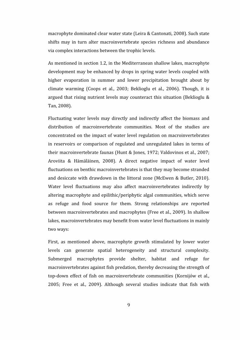
As mentioned in section 1.2, in the Mediterranean shallow lakes, macrophyte

development may be enhanced by drops in spring water levels coupled with

higher evaporation in summer and lower precipitation brought about by

climate warming (Coops et al., 2003; Beklioglu et al., 2006). Though, it is

argued that rising nutrient levels may counteract this situation (Beklioglu &

Tan, 2008).

Fluctuating water levels may directly and indirectly affect the biomass and

distribution of macroinvertebrate communities. Most of the studies are

concentrated on the impact of water level regulation on macroinvertebrates

in reservoirs or comparison of regulated and unregulated lakes in terms of

their macroinvertebrate faunas (Hunt & Jones, 1972; Valdovinos et al., 2007;

Aroviita & Hämäläinen, 2008). A direct negative impact of water level

fluctuations on benthic macroinvertebrates is that they may become stranded

and desiccate with drawdown in the littoral zone (McEwen & Butler, 2010).

Water level fluctuations may also affect macroinvertebrates indirectly by

altering macrophyte and epilithic/periphytic algal communities, which serve

as refuge and food source for them. Strong relationships are reported

between macroinvertebrates and macrophytes (Free et al., 2009). In shallow

lakes, macroinvertebrates may benefit from water level fluctuations in mainly

two ways:

First, as mentioned above, macrophyte growth stimulated by lower water

levels can generate spatial heterogeneity and structural complexity.

Submerged macrophytes provide shelter, habitat and refuge for

macroinvertebrates against fish predation, thereby decreasing the strength of

top-down effect of fish on macroinvertebrate communities (Kornijów et al.,

2005; Free et al., 2009). Although several studies indicate that fish with

10

smaller size aggregate in high numbers within macrophytes in warm lakes

(Meerhoff, 2006), dense vegetation may still act as a potential refuge for

macroinvertebrates.

Secondly, various macroinvertebrate communities may utilize macrophytes

and periphyton as important food sources. Periphyton is a complex

community composed of algae, protozoa, fungi, bacteria, animal inorganic

matter and organic detritus that is attached to the substrates in the water

column, and periphyton growing on submerged macrophytes is called

epiphyton (Wetzel, 2001; Jones & Sayer, 2003). Epiphyton and fresh

macrophyte tissues make up an important part of the diets of some grazers.

Shredders and deposit feeders feed on detritus formed by decaying epiphytic

algae and macrophytes (Kornijów et al., 1995; Diehl & Kornijów, 1998).

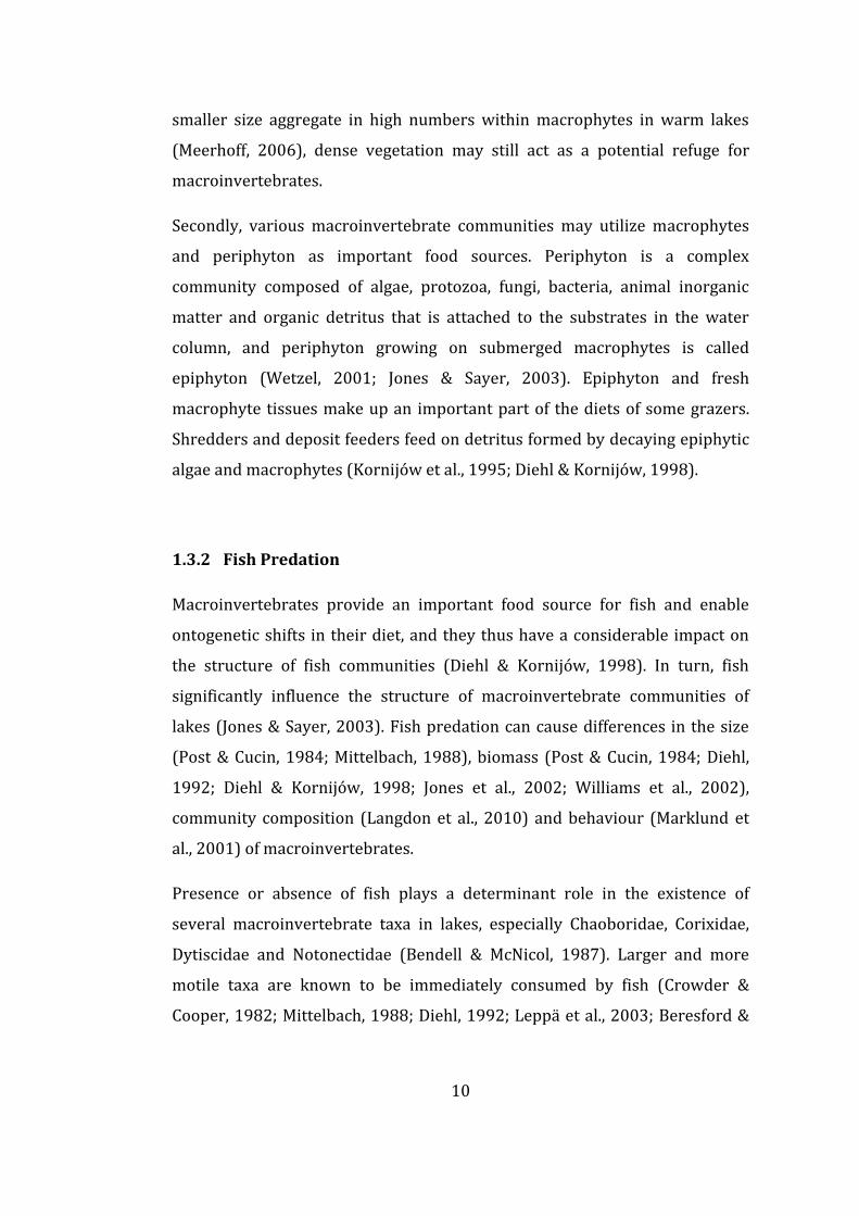
1.3.2 Fish Predation

Macroinvertebrates provide an important food source for fish and enable

ontogenetic shifts in their diet, and they thus have a considerable impact on

the structure of fish communities (Diehl & Kornijów, 1998). In turn, fish

significantly influence the structure of macroinvertebrate communities of

lakes (Jones & Sayer, 2003). Fish predation can cause differences in the size

(Post & Cucin, 1984; Mittelbach, 1988), biomass (Post & Cucin, 1984; Diehl,

1992; Diehl & Kornijów, 1998; Jones et al., 2002; Williams et al., 2002),

community composition (Langdon et al., 2010) and behaviour (Marklund et

al., 2001) of macroinvertebrates.

Presence or absence of fish plays a determinant role in the existence of

several macroinvertebrate taxa in lakes, especially Chaoboridae, Corixidae,

Dytiscidae and Notonectidae (Bendell & McNicol, 1987). Larger and more

motile taxa are known to be immediately consumed by fish (Crowder &

Cooper, 1982; Mittelbach, 1988; Diehl, 1992; Leppä et al., 2003; Beresford &

11

Jones, 2010; Boll, 2010). Thus, some aquatic insect assemblages unique to

naturally fishless lakes have been identified as bioindicators of fish absence

(Schilling et al., 2009). Besides, macroinvertebrates are also used in

determination of naturally fishless lakes by palaeolimnological techniques

(Schilling et al., 2008).

Effects of fish predation on the abundance, richness and size distribution of

macroinvertebrates have been studied in a number of enclosure and

exclosure experiments (Brönmark, 1994; Batzer et al., 2000) but only a few of

these studies principally consider the nonmolluscan macroinvertebrates (i.e.

those other than herbivorous mollusks such as snails).

Fish predation pressure on macroinvertebrates can induce trophic cascades.

Fish may indirectly promote epiphyton growth by preying upon macrophyte-

associated grazing macroinvertebrates, such as snails (Jones & Sayer, 2003).

In a nutrient-rich lake, this may trigger a shift to turbid state via out-shading

of submerged macrophytes by periphyton (Scheffer et al., 1993).

As a climate change scenario, diminishing of piscivorous fish and in turn

reduced top-down control on plankti-benthivores and higher degree of

omnivory, longer spawning season with declining latitude, fish with smaller

size, frequent reproduction, higher specific metabolic and excretion rates may

imply higher predation pressure on macroinvertebrates with rising

temperatures (Meerhoff, 2006).

1.4 Scope of the Study

Mesocosm approach is a valuable tool for understanding the responses of

community structures to various factors by allowing control and

manipulation of parameters together with replication. The mesocosm

experiment was carried out with the main scope of determining the individual

12

and combined effects of water level fluctuations and fish predation pressure

on the ecosystem dynamics and growth of submerged macrophytes in semi-

arid shallow eutrophic lakes. Bucak (2011) showed that water level was

critical for submerged plant growth; the decrease in water levels and a

corresponding increase in underwater light availability compensated for the

unfavourable effects of fish on macrophyte development.

Accordingly, this thesis study aims to elucidate the relative influences of

water level changes and fish on periphyton growth and macroinvertebrates

by manipulating fish presence at different water levels in the in situ

mesocosms. We hypothesized that macroinvertebrate community structure

would be adversely affected by top-down control whereas a decline in water

level and a corresponding macrophyte growth and periphyton development

would, even at presence of fish predation, favor macroinvertebrates by

providing refuge and food source.

In order to test this hypothesis, the experiment was carried out in a shallow

Mediterranean lake, Lake Eymir, using mesocosms constructed at three

different depths reflecting a possible water level fluctuation in the presence

and absence of fish.

13

CHAPTER 2

MATERIALS & METHODS

2.1 Study Site

The mesocosm experiment was conducted in Lake Eymir. Lake Eymir is a

eutrophic shallow lake located south of Ankara, in the Central Anatolia Region

of Turkey (39 57 N, 32 53 E) (Beklioglu et al., 2003). The morphometric

and hydrological characteristics of the lake are summarized in Table 1.

The region experiences the Central Anatolian semi-arid climatic conditions,

the characteristics of which are hot and dry summers, the precipitation

mostly falling in winter and spring. Accordingly, minimum water levels occur

during summer because of evaporation, and maximum depths are reached

during autumn-winter as a result of intense rainfall and snow fall. Frosts are

common during winter months. Average annual air temperature and

precipitation are 21.5 ± 0.8C and 384 ± 104 mm, respectively, for a period of

thirty years (1975-2006) (Özen et al., 2010). The lake experienced rainfall at

the beginning of the summer season, but occasional showers towards the end

of the sampling period, with evaporation becoming more significant in

parallel with the rising temperatures.

A nearby larger shallow lake, Lake Mogan is interconnected to the

downstream Lake Eymir. The outflow from Lake Mogan constitutes the main

inflow of Lake Eymir (“E inflow I” in Figure 1) (Beklioglu et al., 2003), though

14

the canal connecting the two lakes had not been flowing for the last few years

including the sampling period. Another inflow to the lake is Kışlakçı Brook (“E

inflow II” in Figure 1), which feeds the lake in late winter and spring, and

dries in summer. The water leaves via an outflow at the northern tip of Lake

Eymir (“E outflow” in Figure 1).

Table 1: Morphometric and hydrological characteristics of Lake Eymir (Beklioglu et al., 2003; Özen et al., 2010)

Catchment area 971 km2

Altitude 900 m a.s.l.

Surface area 1.20 – 1.25 km2

Volume 3.88×106 m3

Mean depth 2.6 – 3.2 m

Maximum depth 4.3 – 6 m

Shoreline 13 km

Hydraulic retention time 0.2 – 13.5 yr

Water level fluctuation

(mean amplitude of the period 1993–2007) 0.9 ± 0.3 m a.s.l.

More than half a century ago, Lake Eymir was in a clear water state,

dominated by dense submerged plant beds (mainly Charophytes, colonization

depth of which reached a maximum of 6-7 m out of 8 m of maximum water

depth) and nine Cladocera species, including three species of large-bodied

daphnids (Geldiay, 1949). At the time, a Secchi disc transparency of more than

4 m was measured in summer (Geldiay, 1949). Nonetheless, untreated

sewage effluent discharge to the main inflow resulted in a decrease in lake

water quality after 1970s. Total phosphorous (TP), dissolved inorganic

nitrogen (DIN), chlorophyll-a and suspended solids (SS) concentrations

remained at very high levels and Secchi disc depth was low until the sewage

effluent diversion in 1995. The diversion caused a significant decrease in TP

and DIN concentrations, but the water quality and submerged plant coverage

15

remained low (Beklioglu et al., 2003). Following the sewerage diversion, the

lake was subjected to biomanipulation between 1998 and 1999. About half of

the planktivorous tench (Tinca tinca, Linnaeus 1758) and the benthivorous

common carp (Cyprinus carpio, Linnaeus 1758) stock was taken out of Lake

Eymir, which had a considerable effect on water quality (Beklioglu et al.,

2003). Lowered chlorophyll-a and inorganic SS concentrations and enhanced

Secchi disc depth resulted in the expansion of surface submerged macrophyte

coverage up to 40-90% beginning from 2000 until 2003 (Beklioglu & Tan,

2008). Upon the shift of the lake back to turbid water state in 2004 due to the

increase in benthi-planktivorous fish stock, and the disappearance of

submerged plants, a second biomanipulation attempt was undertaken in

2006-2007. Removal of tench and common carp restored the lake water

quality, however poor macrophyte coverage persisted (Özen et al., 2010).

Currently, the fish stock is dominated by Tinca tinca, Cyprinus carpio and

stone moroko, Pseudorasbora parva (Temminck & Schlegel, 1846). The

macrophyte community is mainly composed of sago pondweed, Potamogeton

pectinatus (Linnaeus, 1753) and Najas sp. The phytoplankton community is

dominated by chlorophytes during the clear water period and by

cyanobacteria during the turbid period. Daphnia pulex (De Geer, 1776) and

Arctodiaptomus bacillifer (Koelbel, 1885) largely dominates the zooplankton

community. The dominant emergent plant is common reed, Phragmites

australis (Cavanilles) Trinius ex Steudel on the shoreline (Beklioglu et al.,

unpublished data).

16

Figure 1: Inflows and outflows of the study site, Lake Eymir, and its upstream lake, Lake Mogan, and the location of the lakes on the map of Turkey (taken from Özen et al., 2010)

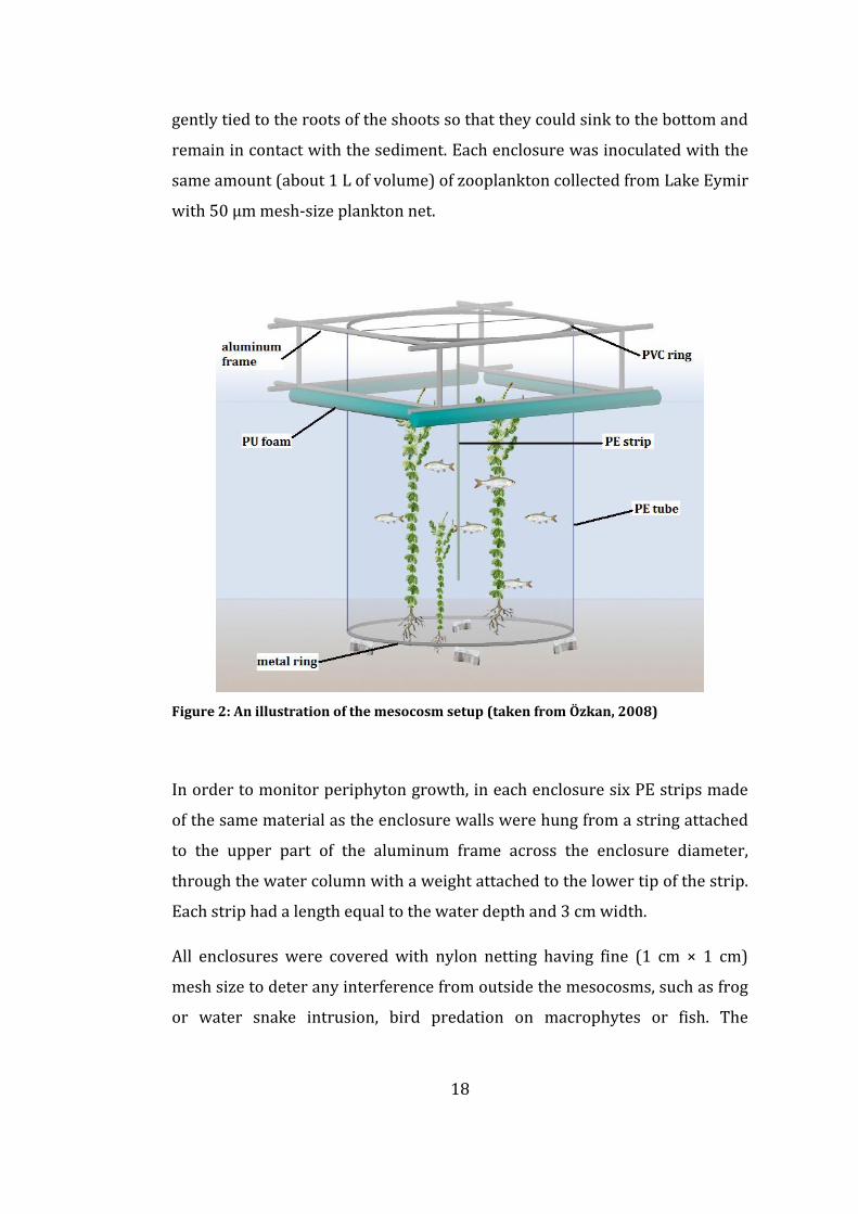
2.2 Experimental Setup: Mesocosms

The experimental setup consisted of cylindrical enclosures that were isolated

from the lake, but exposed to the lake sediment and the atmosphere. Each

enclosure had 1.2 m diameter. The wall of each enclosure was made of

transparent, nylon-reinforced impermeable polyethylene (PE) tube with 0.18

mm thickness so as to enable the penetration of sunlight through the water

column inside. The PE tubes were attached to metal rings on the lower end

and to polyvinyl chloride (PVC) rings on the upper end by using cable ties and

duct tape. The bottom rings were manually extended approximately 0.3 m

17

into the muddy sediment by scuba divers. The top rings were kept floating 0.3

m above the water surface by aluminum floating frames. Each segment of the

frame had a dimension of 1.2 m × 1.2 m × 0.3 m (Özkan, 2008) and the whole

frame consisted of 4 segments on two rows, making up a structure with 5 m

length and 2.5 m width. The lower part of the aluminum frame was supported

with elongated polyurethane (PU) foams to enable buoyancy of the frame and

the attached upper rings of the enclosures above the lake surface. The

experimental setup was kept stable in the lake by fixing the frames from each

corner to concrete bricks placed at the lake bottom using durable ropes. An

enclosure is illustrated in Figure 2.

The enclosures and the aluminum frame were constructed on land and

transported to the experiment location by means of an inflatable boat. All

natural vegetation was carefully removed from the lake bottom by scuba

divers using hand rakes at each mesocosm site prior to the placement of the

experimental setup. Following the placement and anchoring of the aluminum

frames, the enclosures were lowered one by one through each segment of the

frame into the water and their top rings were fixed to the upper part of the

frame using cable ties by scuba divers. Fish intrusion into the enclosures was

prevented during the construction and checked by scuba divers. After the

establishment of the enclosures, the setup was left for one week prior to the

first sampling so that the turbidity arising from the mesocosm asemblage

could settle down and the water column become stable. The enclosures were

carefully checked for possible fish presence using underwater binoculars in

the meantime.

Potamageton pectinatus, a common macrophyte species of the lake’s flora,

was harvested from the lake. Ten shoots of P. pectinatus were transplanted to

each enclosure. Each of them had healthy roots, similar length and number of

shoots in order to achieve similar initial plant densities in the enclosures.

Pebbles were placed in small nylon bags and strings stamped to them were

18

gently tied to the roots of the shoots so that they could sink to the bottom and

remain in contact with the sediment. Each enclosure was inoculated with the

same amount (about 1 L of volume) of zooplankton collected from Lake Eymir

with 50 µm mesh-size plankton net.

Figure 2: An illustration of the mesocosm setup (taken from Özkan, 2008)

In order to monitor periphyton growth, in each enclosure six PE strips made

of the same material as the enclosure walls were hung from a string attached

to the upper part of the aluminum frame across the enclosure diameter,

through the water column with a weight attached to the lower tip of the strip.

Each strip had a length equal to the water depth and 3 cm width.

All enclosures were covered with nylon netting having fine (1 cm × 1 cm)

mesh size to deter any interference from outside the mesocosms, such as frog

or water snake intrusion, bird predation on macrophytes or fish. The

19

establishment phases of the mesocosm and the close-up view of an enclosure

are given in Figure 3 and Figure 4, respectively.

The mesocosm experiment was proposed as 2 × 3 full factorial replicated

block design with four replicate enclosures per treatment, by leaving fishless

versus adding fish to the enclosures established at three different water

depths; 0.8 m, 1.6 m and 2.3 m, corresponding to low, medium and high water

levels, respectively. The replicated treatments were distributed randomly in

the floating frames at each water level. The frames at each depth included 8

enclosures, making up a total of 24 enclosures. The locations of the

mesocosms are presented in Figure 5 showing the Google Earth image of Lake

Eymir.

Fish were stocked to the enclosures after the first sampling. At each depth,

twelve omnivorous–planktivorous fish from the lake’s fauna, i.e. six tench,

Tinca tinca and six bleak, Alburnus escherichii (Steindachner, 1987) having an

average size of 6 cm were added to four replicates corresponding to the

typical fish density of Lake Eymir (Beklioglu & Tan, 2008), and the other four

replicates were left without fish. Fish were caught from the native

populations in Lake Eymir by a sweep net and left in a keepnet for an

adequate time before stocking in order to relieve the stress caused by fishing.

The survival of fish in the enclosures was visually monitored in the course of

the experiment using underwater binoculars. Dead fish were replaced with

new ones when required.

20

Figure 3: Steps in mesocosm construction a) setting up cylindrical enclosures, b) assembling aluminum frames, c) attaching PU foams to frames, d) placing frames on site, e-f) installing and fixing mesocosms, g) planting macrophyte shoots, h) covering mesocosms with netting

a b

c d

e f

h g

21

As explained above, the experimental setup was established as a full factorial

replicated block design, having two fish treatments and three water levels,

with four replicates. However, three replicates in the fishless treatment at 2.3

m depth had to be cancelled due to complications encountered after the fifth

sampling, and the only remaining replicate was not sampled during the rest of

the experiment. Therefore, the results concerning the enclosures at 2.3 m are

excluded in this study. Hereafter, the enclosures established at 0.8 m will be

considered as “low water” (LW) and the ones at 1.6 m as “high water” (HW).

The treatments with fish will be indicated by (+) sign while the fishless

treatments will be indicated by (–) sign.

Figure 4: a) View from HW enclosures, b) Close-up view of a LW enclosure

Figure 5: Map of Lake Eymir and the locations of the mesocosms (Google Earth, 2011)

a

b

22

2.3 Sampling and Processing

The mesocosm experiment was conducted between May 26 – October 2, 2009

for four months so that the effects of different water levels and fish predation

on submerged macrophyte growth could be observed in Lake Eymir. The

sampling dates are given in Table 2. All samplings were performed from a

small boat. The mesocosms were sampled for physical, chemical and

biological parameters weekly in the first five samplings, and biweekly during

the rest of the experiment. The first (pretreatment) sampling was performed

prior to stocking of fish as a control tool to confirm the similarity of the initial

conditions among the treatments and the replicates. On each sampling

occasion, additional samples from outside the mesocosms at each water depth

(from the open lake) were taken in addition to the samples in the mesocosms.

Table 2: Sampling dates

Sampling

1 2 3 4 5 6 7 8 9 10 11

Date

01

.06

.20

09

09

.06

.20

09

15

.06

.20

09

22

.06

.20

09

30

.06

.20

09

13

.07

.20

09

27

.07

.20

09

06

.08

.20

09

17

.08

.20

09

10

.09

.20

09

24

.09

.20

09

Dissolved oxygen (DO) concentration, temperature, conductivity, total

dissolved solids (TDS), salinity and pH were measured just below the water

surface and at 0.5 m intervals (or 0.25 m intervals where necessary) through

the water column with a YSI 556 MPS (Multi-Probe System) (Yellow Springs

Incorporated, OH, U.S.A.) in each sampling.

Water depth, Secchi disc depth, percent macrophyte and filamentous algae

coverage were also recorded for each enclosure. Water depth was measured

23

using both a Speedtech SM-5 Depthmate Portable Sounder Depth Meter and a

sinker for maximum accuracy. Secchi depth was measured using a Secchi disc,

paying attention to performing the measurements at the same time of the day

for the same replicates. Plant volume infested (% PVI) for macrophyte

development was calculated using water depth, average macrophyte height

and surface coverage using the formula: PVI = % coverage × average height /

water depth. Coverage estimation was performed by visually dividing the

enclosure into quarters and estimating the area of the enclosure covered by

plants (Canfield et al., 1984).

A 4 L composite sample was taken from the water column at each enclosure

with a tube, avoiding disturbance to the periphyton strips, macrophytes or

the sediment. A 0.5 L subsample of the composite water sample was taken for

water chemistry analyses. A 0.4 L subsample was taken for suspended matter

(SS) and chlorophyll a (chl-a) analyses. A 0.05 L subsample was preserved on

site with 2 % Lugol’s solution for phytoplankton identification. 3 L of the

composite water sample was filtered through a 20-μm mesh size for

zooplankton identification and preserved on site with 4 % Lugol’s solution. In

the field, all water chemistry, SS and chl-a samples were kept at dark and cold.

They were put in the freezer as soon as arriving at the laboratory and kept

frozen until the analyses have been carried out.

Starting from the third week, PE strips were sampled biweekly for periphyton

chl-a analyses. In each sampling, one periphyton strip was taken out of the

enclosure at a time with care not to disturb the attached periphyton. Two

sections of the strip, each having 0.1 m length, located at 0.1–0.2 m below the

water surface and 0.1–0.2 m above the lake bottom were cut with a scissor

and kept in zip-lock bags in the dark. The remainder of the strips were also

preserved in zip-lock bags in case of need for further analyses. They were

frozen immediately upon arrival at the laboratory.

24

Benthic macroinvertebrate samples were taken before the start of the

experiment, in the middle and at the end of the experiment. The dates of

macroinvertebrate sampling are given in Table 3. Three replicates of the

uppermost 10 cm of the sediment cores taken from each enclosure with a

Kajak sediment core sampler having an internal diameter of 5.2 cm (Figure 6)

were pooled together and put in plastic jars in the field. In the lab, they were

sieved through 500 μm and 212 μm mesh sizes by rinsing the muddy fraction

with tap water. However, no specimens were retained on the sieve with 500

μm mesh size. The benthic macroinvertebrates retained on the 212 μm mesh-

size sieve were preserved in 70% ethanol for identification.

Macrophyte-associated macroinvertebrates were sampled only at the end of

the experiment. The submerged macropytes grown at each enclosure were

harvested at the end of the experiment using a hand rake. They were slowly

taken out of water with care not to disturb the associated macroinvertebrates

while a sieve was placed below them. The macropytes were taken into zip-

lock bags. In the laboratory, they were thoroughly washed with tap water and

the washing water was sieved through 500 μm and 212 μm mesh sizes to

collect the associated macroinvertebrates. However, no specimens were

retained on the sieve with 500 μm mesh size. The macrophyte-associated

macroinvertebrate samples were preserved in 70% ethanol for identification.

The macrophytes cleaned from the associated periphyton and

macroinvertebrates were kept for dry weight determination.

The biomass of macrophyte-associated periphyton (hereafter called

epiphyton) in each enclosure was determined at the end of the experiment.

Three randomly chosen healthy shoots of each macrophte species of 10 cm

length at least 5 cm under the water surface were carefully cut off, to avoid

epiphyton disturbance and transferred into a PE bottle filled with tap water.

Epiphyton was detached by shaking vigorously the bottle manually. Certain

amount of the macrophyte-free water was filtered through Whatman GF/C

25

glass microfiber filter (Whatman International, Maidstone, U.K.) and the

filters were submerged in ethanol for extraction (Jespersen & Christoffersen,

1987) in order to calculate the chl-a content of the epiphyton samples.

Sediment samples were taken with a Kajak corer at the end of the experiment

for organic and carbonate content estimation of the sediment.

Table 3: Macroinvertebrate sampling dates

Sampling

Date Sampled material

Initial sampling 26–27.05.2009 Benthic macroinvertebrates

Middle sampling 11–13.08.2009 Benthic macroinvertebrates

Final sampling

29–30.09.2009 Benthic macroinvertebrates

02.10.2009 Macrophyte-associated

macroinvertebrates

Figure 6: a) Kajak core sampler, b) View from benthic macroinvertebrate sampling

a

b

b

26

2.4 Laboratory Analysis

The water chemistry analyses were carried out immediately after thawing of

the frozen samples. Total phosphorus (TP) and soluble reactive phosphorus

(SRP) concentrations of the water samples were determined using standard

methods based on molybdenum blue complex formation. Acid hydrolysis

method was performed for TP analysis in unfiltered samples, and molybdate

reaction method for SRP analysis in filtered samples (Mackereth et al., 1978).

Analyses of the nitrogen-compounds, namely total nitrogen (TN), ammonium

(NH4-N) and nitrite-nitrate (NO2-N and NO3-N) were carried out with a

continuous flow Skalar Autoanalyzer (San++ Automated Wet Chemistry

Analyzer, Skalar Analytical, B.V., Breda, The Netherlands) following the

standart methods (Krom, 1980; Searle, 1984; Houba et al., 1987; Kroon,

1993). All of the water chemistry analyses were conducted with two

replicates of each sample.

Alkalinity analysis was performed with HCl titration of the samples using

phenolphthalein and BDH indicators (Mackereth et al., 1978). Silicate content

of the filtered samples was determined with molybdate reaction method

(Golterman et al., 1978).

For estimation of chl-a pigment content of phytoplankton and amount of SS,

known volumes of water samples were filtered onto Whatman GF/C glass

microfiber filters. SS was determined as mg/L after drying the filter papers at

105C for 12 hours and weighing (Clesceri et al., 1998). Chl-a was determined

spectrophotometrically with ethanol extraction method at 663 and 750 nm

wavelengths according to Jespersen & Christoffersen (1987) with triple

replication. The same methodology was applied for the estimation of chl-a

concentration associated with the periphyton strips.

27

The macropytes free of the associated periphyton and macroinvertebrates

were dried at 105C for 24 hours for determination of the macrophyte dry

weight at the end of the experiment.

Sediment samples taken at the end of the experiment were treated according

to the sequential loss on ignition (LOI) procedure (Dean, 1974; Heiri et al.,

2001) for determining the water, organic matter and carbonate content of the

sediment. Approximately 1 cc of the sediment samples taken from each

enclosure were placed in preweighed ceramic crucibles and weighed. LOI of

the samples was determined by measuring the weight loss after each heating

step; i.e. 12 hours at 105°C to estimate the water content, then 2 hours at

550°C to estimate the organic matter content and finally, 4 hours at 925°C for

carbonate content estimation. The crucibles were kept in a desiccator to cool

completely before all weighing sessions.

The benthic macroinvertebrate samples were counted and identified under

the stereo microscope (Leica MZ12.5, Leica MZ16 and Leica M125) at highest

100× magnification to the lowest taxonomic level possible following keys of

Macan (1972), Quigley (1977), Fitter & Manuel (1995) and Nilsson (1996,

1997).

Since the macrophyte-associated macroinvertebrate samples contained great

amounts of coarse particulate organic matter (CPOM) such as filamentous

algae and plant pieces, samples were painstakingly cleaned of these nuisances

on a sorting tray by visual checking with the aid of a magnifying glass. The

samples were examined twice in order not to miss any small specimens.

Because picking macroinvertebrates from CPOM-rich samples was a laborious

job and this subsequently required a time-consuming sorting procedure,

three out of four replicates from LW+ and LW– treatments were counted

together with one HW+ and two HW– treatments in which plants had

developed (i.e. a total of two samples were not counted). After this

preliminary sorting process, the collected macroinvertebrates were counted

28

and identified under the stereo microscope (Leica MZ16 and Leica M125) at

highest 100× magnification using the same keys for taxonomical

identification.

Subsampling method was not employed in order to avoid substantial

information loss and the whole samples were handled for counting (Vinson &

Hawkins, 1996). Part of the benthic macroinvertebrate samples were counted

and identified at National Environmental Research Institute of Denmark;

macrophyte-associated macroinvertebrates and the rest of the benthic

macroinvertebrates were counted and identified at METU Limnology

Laboratory.

2.5 Statistical Analysis

The statistical analyses were performed with SigmaStat® release 3.5 (Systat

Software, San Jose, CA/Richmond, CA, USA) and SAS® (Statistical Analysis

Software) release 9.2 (SAS Institute Inc, Cary, NC) statistical softwares. The

general linear model (GLM) procedure of SAS was used for repeated

measures of two-way analysis of variance (RM two-way ANOVA) (Bucak,

2011) and SigmaStat was used for all the other analyses. Differences were

considered statistically significant at the p < 0.05 level in all statistical

analyses.

To assess similarity of the starting conditions in the mesocosms, initial

sampling data regarding the physico-chemical parameters and chl-a were

tested in one-way ANOVA, with water level as a fixed factor (Bucak, 2011).

Since the initial sampling of benthic macroinvertebrates was also performed

prior to fish addition, data regarding this sampling event was analysed with

one-way ANOVA to test if there was any significant difference among the LW

and HW treatments. The middle and final sampling data of benthic

macroinvertebrates, epiphyton chl-a, macrophyte DW and macrophyte-

29

associated macroinvertebrate data were analysed with two-way ANOVA with

water level and fish presence/absence as crossed fixed factors. In addition,

the middle and final sampling data of benthic macroinvertebrates were

handled using paired t-test (with Bonferroni correction of α = 0.0125) in

order to detect any significant effect of time between the two consecutive

sampling events. Periphyton chl-a and PVI data were analysed with RM two-

way ANOVA (Bucak, 2011). LOI data was tested in one-way ANOVA to see

whether the sediment characteristics were significantly different in the LW

and HW treatments. Tukey pairwise comparison test with 95% confidence

level was applied in all statistical tests if the parameters showed significant

difference.

Because of the nature of species-sample matrices with a high prevalence of

zero entries, community data are likely to encounter major problems in

fulfilling the assumptions for parametric statistics (Baumgärtner, Mörtl &

Rothhaupt, 2008). Normal distribution of data was checked by the

Kolmogorov–Smirnov goodness of fit procedure or relevant diagnostic plots.

Data that violated normality or heteroscedasticity assumptions of ANOVA

were logarithmic, square root or reciprocal transformed. The parameters that

failed the assumptions even after log10 (x+1), √x and 1/(x+1) transformations

were analysed using the non-parametric analogues of the above mentioned

parametric tests, namely Kruskal-Wallis and Friedman tests.

30

CHAPTER 3

RESULTS

3.1 Physico-chemical Parameters

During the course of the experiment, a significant water level drop was

observed in all of the mesocosms, both LW and HW (Figure 7). At the start of

the experiment, the water depth in LW enclosures ranged between 0.80-1 m,

and in HW enclosures between 1.6-1.7 m. The difference in water depths

between the initial and last sampling dates was 0.46 ± 0.03 m [mean ±

standard deviation (SD)]. Water level decreased dramatically onward the fifth

sampling, coinciding with the high surface water temperatures exceeding

26°C.

Figure 7: Change in water levels of the mesocosms over the course of the experiment

31

Initial conditions for all parameters are summarised in Table 4 according to

the results of one-way ANOVA between LW and HW. Initial values of

conductivity, TP and SRP differed significantly among the LW and HW

treatments. RM two-way ANOVA results for all physico-chemical parameters

and some of the biological variables are summarised in Table 5. The physico-

chemical parameters are discussed thoroughly in Bucak (2011).

Table 4: One-way ANOVA results showing the influence of water level on the initial conditions of the parameters measured in time series and the parameters sampled once (denoted by asterisks) in the mesocosms (ns denotes a non-significant difference with p > 0.05.) (Bucak, 2011)

Parameter p

Conductivity <0.05

Suspended solids ns

pH ns

TP 0.003

SRP <0.001

TN ns

NO2-N and NO3-N ns

chl-a ns

Organic matter content (LOI at 550°C) * ns

Carbonate content (LOI at 925°C) * ns

As an indication of the extent of light penetration through the water column,

the ratio of Secchi disc depth to average depth was used. Both water level and

fish had a significant impact on this ratio (RM two-way ANOVA; p=0.004 and

p=0.0001, respectively; Table 5) (Bucak, 2011). The Secchi disc

depth/average depth ratio was higher in the fishless mesocosms through the

experiment and converged to 1 (meaning Secchi disc depth was almost equal

to the water level) in LW- mesocosms as a result of the enhanced underwater

light penetration and decrease in water levels (Figure 8).

32

a) b)

Figure 8: Ratio of Secchi disc depth to average depth of the mesocosms a) change over the course of the experiment, b) comparison of all treatments at the end of the experiment

3.2 Macrophytes, Epiphyton and Periphyton

Submerged macrophyte development remained very low in the HW

mesocosms over the course of the experiment (Table 5; Figure 9). However,

extensive macrophyte growth occurred in both the LW- and LW+ mesocosms,

especially towards the end of the experiment (Table 5; Figure 9).

Macrophytes grew not in all of the HW mesocosms and accordingly, the

associated macroinvertebrates and epiphyton could only be sampled in three

replicates of the HW mesocosms (i.e. two replicates in HW- and one replicate

in HW+). PVI was significantly affected by both water level and fish (RM two-

way ANOVA; p<0.0001 and p=0.0001, respectively; Table 5) (Bucak, 2011).

Water level, fish and their interaction also significantly affected the dry

weight of macrophytes harvested at the end of the experiment (two-way

ANOVA; p<0.0001, p=0.0243, and p=0.019, respectively; Table 5 and Figure 9)

(Bucak, 2011). LW- treatments had the highest macrophyte dry weight and

%PVI at the end of the experiment.

33

Table 5: Average values [(mean ± standart error (SE)] of some physico-chemical and biological parameters measured in the mesocosms and the results of RM two-way ANOVA (only for macrophyte DW and epiphyton chl-a, which did not have time series data, p values are results of two-way ANOVA) (WL and F denote water level and fish, respectively. ns denotes a non-significant difference with p > 0.05.) (Bucak, 2011)

LW- LW+ HW- HW+ WL F WL*F

Secchi /average depth 0.92 ± 0.14 0.73 ± 0.21 0.84 ± 0.25 0.44 ± 0.21 0.004 0.0001 ns

Conductivity (μs/cm) 2862.2 ± 20.0 2802.1 ± 14.9 2721.4 ± 32.38 2716.8 ± 28.4 <0.0001 ns 0.001

Suspended solids (mg/L) 15.56 ± 1.24 34.02 ± 3.14 12.21 ± 1.36 25.18 ± 2.25 0.0114 <0.0001 ns

Dissolved oxygen (mg/L) 8.08 ± 0.40 6.74 ± 0.47 5.82 ± 0.54 5.38 ± 0.39 0.0005 ns ns

pH 9.04 ± 0.03 8.81 ± 0.02 8.93 ± 0.02 8.88 ± 0.02 ns 0.0011 0.0202

TP (μg/L) 237.4 ± 11.37 269.8 ± 10.28 128.2 ± 10.34 179.2 ± 11.17 <0.0001 0.0128 ns

SRP (μg/L) 114.7 ± 7.59 114.2 ± 9.93 30.5 ± 2.64 41.0 ± 4.70 <0.001 ns 0.0424

TN (μg/L) 1312.3 ± 67.2 1506.8 ± 88.9 1176.3 ± 94.7 1214.6 ± 83.48 <0.001 0.0256 ns

NO2-N and NO3-N (μg/L) 31.88 ± 6.75 49.25 ± 9.16 10.13 ± 1.70 9.85 ± 1.87 0.0005 ns ns

chl-a (μg/L) 15.58 ± 3.71 89.53 ± 14.26 19.35 ± 6.40 47.87 ± 7.31 0.025 <0.001 ns

Upper periphyton chl-a

(μg/cm2)4.87 ± 0.85 5.76 ± 0.75 4.24 ± 0.72 5.05 ± 0.89 ns ns ns

Lower periphyton chl-a

(μg/cm2)3.74 ± 0.51 4.17 ± 0.58 6.014 ± 0.62 2.09 ± 0.38 0.0003 0.0197 0.0046

PVI (%) 43.18 ± 5.16 24.33 ± 5.05 0.40 ± 0.22 1.47 ± 0.34 <0.0001 0.0001 ns

Macrophyte dry weight (g) 121.45 ± 22.64 58.73 ± 6.95 0.18 ± 0.11 1.74 ± 1.74 <0.0001 0.0243 0.019

Epiphyton chl-a

(µg/g macrophyte DW)0.83 ± 0.58 1.60 ± 0.84 7.61 ± 12.62 0.06 ± 0.12 0.01 ns ns

Parametermean ± SD p

33

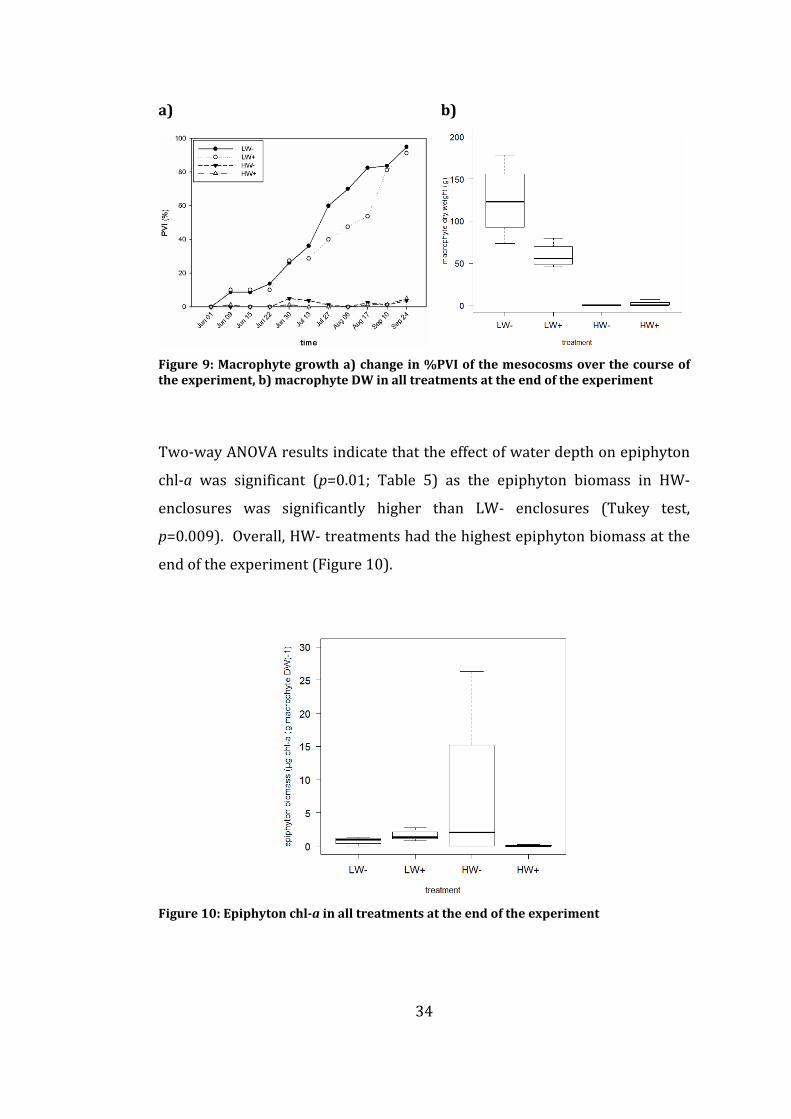
34

a) b)

Figure 9: Macrophyte growth a) change in %PVI of the mesocosms over the course of the experiment, b) macrophyte DW in all treatments at the end of the experiment

Two-way ANOVA results indicate that the effect of water depth on epiphyton

chl-a was significant (p=0.01; Table 5) as the epiphyton biomass in HW-

enclosures was significantly higher than LW- enclosures (Tukey test,

p=0.009). Overall, HW- treatments had the highest epiphyton biomass at the

end of the experiment (Figure 10).

Figure 10: Epiphyton chl-a in all treatments at the end of the experiment

35

RM two-way ANOVA results (Table 5; Figure 11), showed no significant effect

of neither water level nor fish (p>0.1 for both) on chl-a concentrations of the

upper portion of periphyton strips (corresponding to 0.1–0.2 m below the

water surface, hereafter called upper periphyton). On the contrary, both

water level and fish were found to have a significant impact (p=0.0003 and

p=0.0197, respectively) on chl-a concentrations of the lower portion of

periphyton strips (corresponding to 0.1–0.2 m above the lake bottom,

hereafter called bottom periphyton) according to the results of RM two-way

ANOVA (Table 5; Figure 12). In addition, interaction of these two parameters

also significantly affected the bottom periphyton biomass (p=0.0046) as it

was highest in the HW- treatments at the end of the experiment (Figure 12).

a) b)

Figure 11: Upper periphyton chl-a a) change over the course of the experiment, b) comparison of all treatments in the last sampling

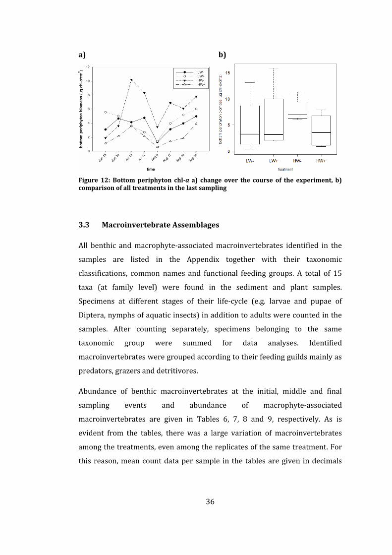
36

a) b)

Figure 12: Bottom periphyton chl-a a) change over the course of the experiment, b) comparison of all treatments in the last sampling

3.3 Macroinvertebrate Assemblages

All benthic and macrophyte-associated macroinvertebrates identified in the

samples are listed in the Appendix together with their taxonomic

classifications, common names and functional feeding groups. A total of 15

taxa (at family level) were found in the sediment and plant samples.

Specimens at different stages of their life-cycle (e.g. larvae and pupae of

Diptera, nymphs of aquatic insects) in addition to adults were counted in the

samples. After counting separately, specimens belonging to the same

taxonomic group were summed for data analyses. Identified

macroinvertebrates were grouped according to their feeding guilds mainly as

predators, grazers and detritivores.

Abundance of benthic macroinvertebrates at the initial, middle and final

sampling events and abundance of macrophyte-associated

macroinvertebrates are given in Tables 6, 7, 8 and 9, respectively. As is

evident from the tables, there was a large variation of macroinvertebrates

among the treatments, even among the replicates of the same treatment. For

this reason, mean count data per sample in the tables are given in decimals

37

(though they show the number of individuals) so as not to underrepresent

rare taxa (i.e. those present only in one or few replicates with very few

individuals). Taxa that were not abundant were also taken into account in the

data analyses because of likelihood of high patchiness and heterogeneity of

macroinvertebrate distribution.

The following parameters were chosen for defining the abundance and

community composition of the macroinvertebrates:

- Density: For benthic macroinvertebrates, individuals found in m2 of

sediment, was calculated by dividing the total number of individuals counted

in a sample by the total surface area of three sediment core samples taken by

Kajak corer (internal diameter of 5.2 cm), assuming that macroinvertebrates

were dwelling the surface of the sediment and not the whole core volume. For

macrophyte-associated macroinvertebrates, density was defined as the

number of individuals per 100 g dry plant biomass. It was calculated by

dividing the total number of individuals counted in a sample by the dry

weight of the macrophytes harvested from that sample.

- Taxa richness: Since all individuals were identified at least to family level,

family level richness was taken as a basis for comparative purposes even

though some individuals could be identified to lower taxonomic levels such as

subfamily or genus.

- Predator density: Density of individuals belonging to predator groups (i.e.

Ceratopogonidae, Chaoboridae, Corixidae, Coenagrionidae, Hygrobatidae,

Hydrophilidae, Dytiscidae) was used as this parameter, together with the

following one, could give insight into the interrelations of different functional

feeding groups.

- Grazer-detritivore density: Density of individuals belonging to grazer (i.e.

Chironomidae, Ephydridae, Baetidae, Aphididae, Planorbidae) and detritivore

(i.e. Lumbricidae, Sminthuridae, Isotomidae) groups were pooled together as

38

the amount of detritus was expected to be higher in the treatments where

substrate for grazers was available.

- Chironomid density: Density of Chironomidae was used to estimate the

grazing pressure exerted on epiphyton and periphyton as chironomids were

usually the dominant taxa among grazers.

- Vulnerable density: Density of individuals belonging to taxa that are

vulnerable to fish predation (i.e. Chaoborus sp., Corixidae, Odonata and

Ephemeroptera) were taken into consideration as these could be a indicative

of fish presence/absence.

Table 6: Abundance (mean ± SD per sample) of benthic macroinvertebrates in all treatments at the initial sampling (Dominant taxa are highlighted by asterisks.)

Taxon Abundance (mean ± SD)

LW- LW+ HW- HW+

Ceratopogoninae* 0.25±0.50 0.00±0.00 15.00±26.70 6.00±4.08

Chaoborus sp. 0.00±0.00 0.00±0.00 0.75±0.96 0.00±0.00

Chironomidae* 3.00±4.08 8.50±8.27 2.25±1.71 3.50±1.00

Brachycera 0.00±0.00 0.00±0.00 0.00±0.00 0.00±0.00

Oligochaeta 0.00±0.00 0.00±0.00 0.00±0.00 0.00±0.00

Corixidae 1.00±2.00 0.50±1.00 0.00±0.00 0.00±0.00

Coenagrionidae 0.00±0.00 1.00±0.00 0.00±0.00 0.00±0.00

Baetidae 0.00±0.00 0.00±0.00 0.00±0.00 0.00±0.00

Hygrobatidae 0.00±0.00 0.00±0.00 0.00±0.00 0.00±0.00

Aphididae 0.00±0.00 0.00±0.00 0.00±0.00 0.00±0.00

39

Table 7: Abundance (mean ± SD per sample) of benthic macroinvertebrates in all treatments at the middle sampling (Dominant taxa are highlighted by asterisks.)

Taxon Abundance (mean ± SD)

LW- LW+ HW- HW+

Ceratopogoninae* 0.00±0.00 0.25±0.50 9.75±12.45 2.25±2.63

Chaoborus sp.* 2.50±2.38 0.00±0.00 2.25±2.22 0.50±1.00

Chironomidae 1.00±1.41 0.50±0.58 1.25±1.26 0.50±1.00

Brachycera 0.00±0.00 0.00±0.00 0.00±0.00 0.00±0.00

Oligochaeta 0.25±0.50 0.75±0.96 0.00±0.00 0.00±0.00

Corixidae* 0.50±1.00 0.25±0.50 36.00±41.86 0.00±0.00

Coenagrionidae 0.00±0.00 0.00±0.00 0.00±0.00 0.00±0.00

Baetidae 1.50±0.71 0.00±0.00 0.00±0.00 0.00±0.00

Hygrobatidae 0.00±0.00 0.00±0.00 0.00±0.00 0.00±0.00

Aphididae 0.00±0.00 0.00±0.00 0.00±0.00 0.00±0.00

Table 8: Abundance (mean ± SD per sample) of benthic macroinvertebrates in all treatments at the final sampling (Dominant taxa are highlighted by asterisks.)

Taxon Abundance (mean ± SD)

LW- LW+ HW- HW+

Ceratopogoninae* 5.00±5.35 5.25±4.50 13.00±14.72 0.50±1.00

Chaoborus sp. 1.75±2.87 0.25±0.50 0.25±0.50 1.00±1.15

Chironomidae 0.25±0.50 1.00±1.15 0.50±0.58 1.25±1.26

Brachycera 0.00±0.00 1.50±1.73 0.00±0.00 0.00±0.00

Oligochaeta 0.25±0.50 0.25±0.50 0.00±0.00 0.00±0.00

Corixidae* 10.25±13.72 0.75±0.96 104.75±123.24

10.25±14.61

Coenagrionidae 1.00±0.00 0.00±0.00 0.00±0.00 0.00±0.00

Baetidae 0.00±0.00 3.00±0.00 0.00±0.00 0.00±0.00

Hygrobatidae 0.00±0.00 1.00±0.00 0.00±0.00 0.00±0.00

Aphididae 0.00±0.00 1.00±0.00 0.00±0.00 0.00±0.00

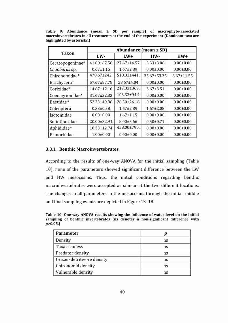
40

Table 9: Abundance (mean ± SD per sample) of macrophyte-associated macroinvertebrates in all treatments at the end of the experiment (Dominant taxa are highlighted by asterisks.)

Taxon Abundance (mean ± SD)

LW- LW+ HW- HW+

Ceratopogoninae* 41.00±67.56 27.67±14.57 3.33±3.06 0.00±0.00

Chaoborus sp. 0.67±1.15 1.67±2.89 0.00±0.00 0.00±0.00

Chironomidae* 478.67±242.79

518.33±441.30

35.67±53.35 6.67±11.55

Brachycera* 57.67±87.78 28.67±4.04 0.00±0.00 0.00±0.00

Corixidae* 14.67±12.10 217.33±369.51

3.67±3.51 0.00±0.00

Coenagrionidae* 31.67±32.33 103.33±94.48

0.00±0.00 0.00±0.00

Baetidae* 52.33±49.96 26.50±26.16 0.00±0.00 0.00±0.00

Coleoptera 0.33±0.58 1.67±2.89 1.67±2.08 0.00±0.00

Isotomidae 0.00±0.00 1.67±1.15 0.00±0.00 0.00±0.00

Sminthuridae 20.00±32.91 8.00±5.66 0.50±0.71 0.00±0.00

Aphididae* 10.33±12.74 458.00±790.68

0.00±0.00 0.00±0.00

Planorbidae 1.00±0.00 0.00±0.00 0.00±0.00 0.00±0.00

3.3.1 Benthic Macroinvertebrates

According to the results of one-way ANOVA for the initial sampling (Table

10), none of the parameters showed significant difference between the LW

and HW mesocosms. Thus, the initial conditions regarding benthic

macroinvertebrates were accepted as similar at the two different locations.

The changes in all parameters in the mesocosms through the initial, middle

and final sampling events are depicted in Figure 13–18.

Table 10: One-way ANOVA results showing the influence of water level on the initial sampling of benthic invertebrates (ns denotes a non-significant difference with p>0.05.)

Parameter p

Density ns

Taxa richness ns

Predator density ns

Grazer-detritivore density ns

Chironomid density ns

Vulnerable density ns

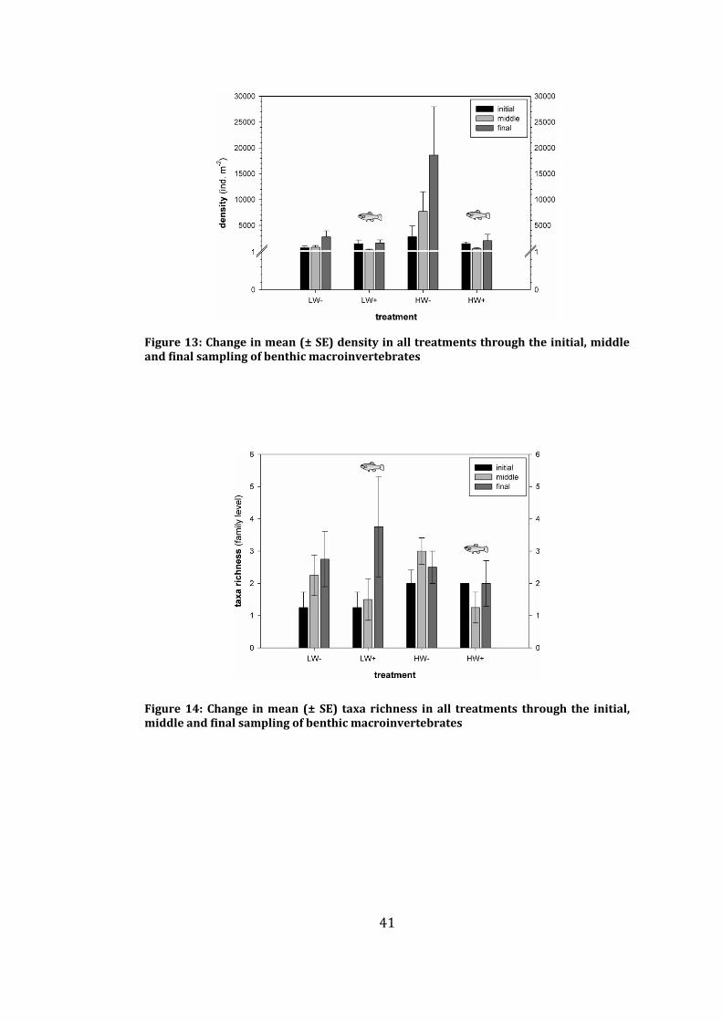
41

Figure 13: Change in mean (± SE) density in all treatments through the initial, middle and final sampling of benthic macroinvertebrates

Figure 14: Change in mean (± SE) taxa richness in all treatments through the initial, middle and final sampling of benthic macroinvertebrates

42

Figure 15: Change in mean (± SE) predator density in all treatments through the initial, middle and final sampling of benthic macroinvertebrates

Figure 16: Change in mean (± SE) grazer-detritivore density in all treatments through the initial, middle and final sampling of benthic macroinvertebrates

43

Figure 17: Change in mean (± SE) chironomid density through the initial, middle and final sampling of benthic macroinvertebrates

Figure 18: Change in mean (± SE) vulnerable density in all treatments through the initial, middle and final sampling of benthic macroinvertebrates

The two-way ANOVA results for the middle sampling of benthic

macroinvertebrates (Table 11) indicate that there was a significant impact of

fish on the density (p=0.045, Figure 19), taxa richness (p=0.042, Figure 20)

and vulnerable density (p<0.001, Figure 21). None of the parameters were

significantly affected by water level. Benthic macroinvertebrate density as

44

well as taxa richness (Tukey test between HW- and HW+ treatments,

p=0.044) was significantly higher in fishless enclosures than the enclosures

with fish. At both LW and HW, vulnerable density was significantly lower in

the mesocosms with fish than fishless mesocosms (Tukey test; p=0.01 and

p=0.002, respectively).

Table 11: Two-way ANOVA results showing the influence of water level, fish and their interaction on the middle sampling of benthic macroinvertebrates (ns denotes a non-significant difference with p > 0.05.)

Parameter p

WL F WL*F

Density ns 0.045 ns

Taxa richness ns 0.042 ns

Predator density ns ns ns

Grazer-detritivore density ns ns ns

Chironomid density ns ns ns

Vulnerable density ns <0.001 ns

Figure 19: Density of benthic macroinvertebrates in all treatments in the middle sampling

45

Figure 20: Taxa richness of benthic macroinvertebrates in all treatments in the middle sampling

Figure 21: Vulnerable density of benthic macroinvertebrates in all treatments in the middle sampling

The two-way ANOVA results for the final sampling of benthic

macroinvertebrates (Table 12) show that there was a significant effect of fish

only on the predator density (p=0.049, Figure 22), as it was significantly

lower in the mesocosms with fish than fishless mesocosms at both LW and

46

HW (Tukey test; p=0.049 and p=0.024, respectively). None of the parameters

were significantly affected by water level.

Table 12: Two-way ANOVA results showing the influence of water level, fish and their interaction on the final sampling of benthic macroinvertebrates (ns denotes a non-significant difference with p > 0.05.)

Parameter p

WL F WL*F

Density ns ns ns

Taxa richness ns ns ns

Predator density ns 0.049 ns

Grazer-detritivore density ns ns ns

Chironomid density ns ns ns

Vulnerable density ns ns ns

Figure 22: Predator density of benthic macroinvertebrates in all treatments in the final sampling

3.3.2 Macrophyte-associated Macroinvertebrates

The two-way ANOVA results for macrophyte-associated macroinvertebrates

(Table 13) indicate that there was a significant impact of water level on the

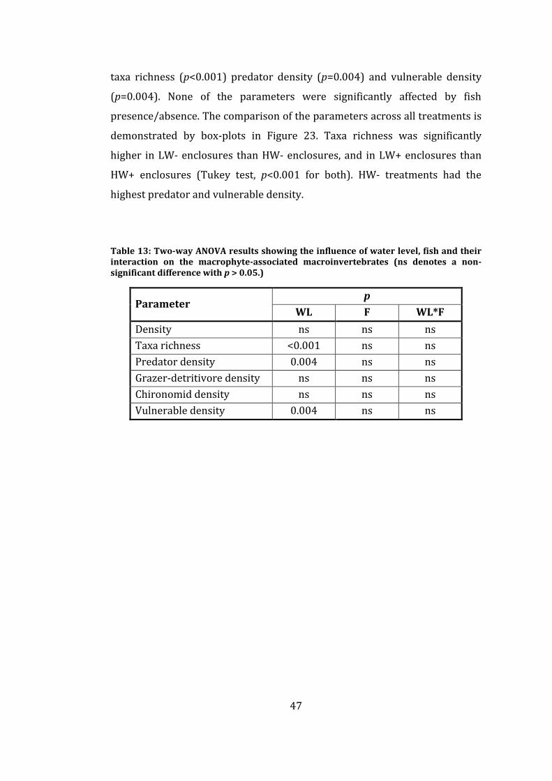
47

taxa richness (p<0.001) predator density (p=0.004) and vulnerable density

(p=0.004). None of the parameters were significantly affected by fish

presence/absence. The comparison of the parameters across all treatments is

demonstrated by box-plots in Figure 23. Taxa richness was significantly

higher in LW- enclosures than HW- enclosures, and in LW+ enclosures than

HW+ enclosures (Tukey test, p<0.001 for both). HW- treatments had the

highest predator and vulnerable density.

Table 13: Two-way ANOVA results showing the influence of water level, fish and their interaction on the macrophyte-associated macroinvertebrates (ns denotes a non-significant difference with p > 0.05.)

Parameter p

WL F WL*F

Density ns ns ns

Taxa richness <0.001 ns ns

Predator density 0.004 ns ns

Grazer-detritivore density ns ns ns

Chironomid density ns ns ns

Vulnerable density 0.004 ns ns

48

a) b)

c) d)

e) f)

Figure 23: Comparison of the parameters for macrophyte-associated macroinvertebrates in all treatments a) total density, b) taxa richness (family level), c) predator density, d) grazer-detritivore density, e) chironomid density, f) vulnerable density

49

CHAPTER 4

DISCUSSION & CONCLUSION

4.1 Discussion

Following the study of Özkan (2008), the mesocosm experiment was

conducted with the purpose of determining the effects of water level

fluctuations and fish predation on submerged macrophyte growth in a semi-

arid shallow eutrophic lake. Submerged plant development being the main

focus of the experiment and the subject of another thesis, its relationship with

physico-chemical variables and nutrient availability under the influence of

water level change and fish presence were thoroughly discussed by Bucak

(2011).

With this thesis, the relative influences of top-down and bottom-up

interactions on periphyton growth and macroinvertebrates were aimed to be

investigated by manipulating fish presence at different water levels in the in

situ mesocosms. Thus, the focus of discussion is on macroinvertebrates in

relation to fish predation and periphyton growth brought about by change in

water levels.

In the summer of 2009, when the experiment was carried out, frequent rain

events were experienced in the first few weeks of June, while temperature

rise became more apparent as from July. This led to increased evaporation

and a corresponding drop of water levels. At the end of the 4-month sampling

50

period, the water level had decreased by an average of 0.46 ± 0.03 m (Figure

7), which is characteristic of the Mediterranean semi-arid climate.

The Secchi disc depth/average depth ratio in the mesocosms differed

significantly under the influence of water level and fish. Underwater light

penetration was higher in the fishless enclosures over the course of the

experiment. Water clarity was higher in LW enclosures and phytoplankton

biomass was lower in the fishless enclosures at the end of the experiment.

The highest Secchi disc depth/average depth ratio was observed in the LW-

treatment (Figure 8).

Both water level and fish had a significant impact on submerged macrophytes.

Macrophyte development occurred in the LW enclosures despite having had

high concentrations of N and P, but not in the HW enclosures. Dry weight of

macrophytes and %PVI were both found to be higher in LW- than LW+

enclosures at the end of the experiment (Figure 9). Plant growth remained

very low in HW- enclosures despite high water clarity, which may be the

result of competition with periphyton for light in the lower part of the water

column (Bucak, 2011).

In accordance with previous studies (Coops et al., 2005; Beklioglu et al. 2006;

Özkan et al., 2010) which suggest that water level is critical for macrophyte

development in semi-arid climatic regions, Bucak (2011) has concluded that

low water levels during growth season might override the adverse effects of

eutrophication and intense top-down control of fish, and allow macrophyte

growth even under poor light availability in the water column.

4.1.1 Epiphyton and Periphyton

The highest epiphyton chl-a was observed in HW- enclosures (Figure 10). The

inverse correlation between invertebrate grazers and epiphyton has been

well documented by exclosure-enclosure and large-scale experiments

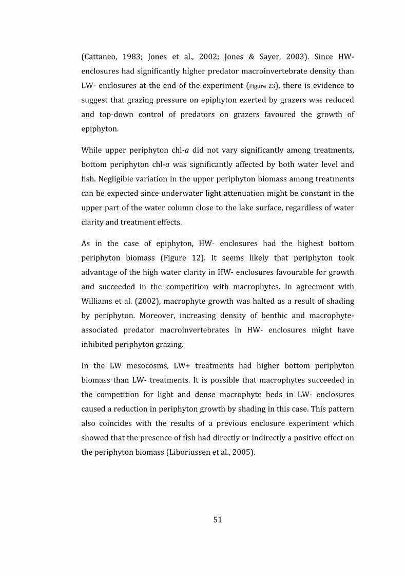
51

(Cattaneo, 1983; Jones et al., 2002; Jones & Sayer, 2003). Since HW-

enclosures had significantly higher predator macroinvertebrate density than

LW- enclosures at the end of the experiment (Figure 23), there is evidence to

suggest that grazing pressure on epiphyton exerted by grazers was reduced

and top-down control of predators on grazers favoured the growth of

epiphyton.

While upper periphyton chl-a did not vary significantly among treatments,

bottom periphyton chl-a was significantly affected by both water level and

fish. Negligible variation in the upper periphyton biomass among treatments

can be expected since underwater light attenuation might be constant in the

upper part of the water column close to the lake surface, regardless of water

clarity and treatment effects.

As in the case of epiphyton, HW- enclosures had the highest bottom

periphyton biomass (Figure 12). It seems likely that periphyton took

advantage of the high water clarity in HW- enclosures favourable for growth

and succeeded in the competition with macrophytes. In agreement with

Williams et al. (2002), macrophyte growth was halted as a result of shading

by periphyton. Moreover, increasing density of benthic and macrophyte-

associated predator macroinvertebrates in HW- enclosures might have

inhibited periphyton grazing.

In the LW mesocosms, LW+ treatments had higher bottom periphyton

biomass than LW- treatments. It is possible that macrophytes succeeded in

the competition for light and dense macrophyte beds in LW- enclosures

caused a reduction in periphyton growth by shading in this case. This pattern

also coincides with the results of a previous enclosure experiment which

showed that the presence of fish had directly or indirectly a positive effect on

the periphyton biomass (Liboriussen et al., 2005).

52

4.1.2 Macroinvertebrates

Highly variable distribution and abundance of several taxa in the enclosures

implied the patchy and heterogeneous existence of macroinvertebrates in

lentic ecosystems (Baumgärtner et al., 2008). For instance, large number of

individuals of a taxon was counted in a replicate while none or very few

individuals belonging to the same taxon were encountered in another

replicate of even the same treatment. Also, it was common to count only a few

individuals of a taxon in a single replicate among all treatments (see Table 6-

Table 9 for raw data). Detecting changes in the fauna requires extensive

efforts to obtain sufficient statistical data (Baumgärtner et al., 2008), so the

macroinvertebrate analysis results in the previous chapter should be

interpreted cautiously. The following discussion on macroinvertebrates was

based on the statistical analysis results as well as the comparison of count

data in order to see more clearly the trends that were not explicit in statistical

analyses.

Initial sampling of benthic macroinvertebrates revealed no significant

difference between the LW and HW mesocosms. Similarity of the initial

conditions at these two distant locations were expected since the sediment

characteristics (LOI results for organic matter and carbonate content

estimation) were also similar for both LW and HW mesocosms, and the lake

bottom was cleared of vegetation prior to the placement of the mesocosms.

Fish had a significant effect on total density, taxa richness and vulnerable

density in the middle sampling (Table 11), and on predator density in the

final sampling (Table 12) of benthic macroinvertebrates. Water level had no

significant impact on any of the parameters in either sampling events. The

trends evident between the two consecutive sampling events (i.e. effect of

time) did not prove to be statistically significant.

The density of benthic macroinvertebrates was highest in HW- enclosures

(Figure 13). Fish-free enclosures had higher density than the enclosures with

53

fish. Benthic macroinvertebrate density remained lower in treatments with

fish throughout the experiment as a result of top-down control of fish. Though

not statistically significant, macroinvertebrate densities showed a

continuously increasing trend in fish-free enclosures over the course of the

experiment whereas a downward unimodal (decreasing and then increasing)

trend was observed in the enclosures with fish. The reason for this may be the

high predation pressure of fish on bare sediment, but in time the predation

pressure might have been diminished by the growth of submerged

macrophytes and their refuge effect.

Fish had a statistically significant impact on taxa richness in the middle

sampling, but not in the final sampling of benthic macroinvertebrates. Taxa

richness was highest in HW- enclosures and higher in fishless treatments in

the middle sampling (Figure 20). But at the end of the experiment, this

difference disappeared and richness increased in LW treatments likely as a

result of the extensive macrophyte coverage in both LW- and LW+ enclosures.

Fish had a significant effect on predator density only in the final sampling of

benthic macroinvertebrates. Predator density was highest in HW- treatments

and had an obviously increasing trend in the fish-free enclosures throughout

the experiment (Figure 15). On the contrary, grazer-detritivore density

decreased in these enclosures where predators increased in abundance

(Figure 16). A similar trend in chironomid density was apparent in fishless

enclosures (Figure 18) as Chironomidae was the most abundant taxon within

the grazer-detritivore group. These results support the evidence that large,

predatory invertebrates are capable of reducing density of their prey (Diehl,

1992; Prejs et al., 1997). The contrasting patterns in the densities of predators

and grazer-detritivores suggest that, in the absence of fish, internal predation

dynamics of macroinvertebrates can be as important in influencing their

community structure as fish predation pressure. Moreover, cascading top-

down effects may have implications for epiphyton and periphyton, as

discussed in the previous section.

54

The density of vulnerable taxa was significantly influenced by fish in the

middle sampling (Figure 21), but not in the final sampling of benthic

macroinvertebrates. It was higher in the fishless enclosures and had an

increasing trend throughout the experiment (Figure 18). The highest

vulnerable density was observed in HW- enclosures. Data revealed that

individuals of taxa known to be vulnerable to fish predation (e.g. Chaoborus

larvae and Corixidae) were more abundant in the mesocosms without fish,

whereas they were rare or absent in the fishless mesocosms (see Table 6-

Table 9 for raw data), indicating that the exclusion of fish from the system

possibly led to an increase in the density of these taxa. This result is in

agreement with Eriksson et al. (1980), who documented that taxa suppressed

by fish predation becomes abundant when fish predation ceases. In addition

to the direct effect of fish predation, exclusion of these large-size selective

predators from the system can also have implications for altering community

composition via replacement of fish by such small-size selective predators

and other aquatic insects, and a consequent shift to invertebrate-dominated

predator-prey systems (Eriksson et al., 1980).

On the other hand, fish did not have any statistically significant effect on

macrophyte-associated macroinvertebrates while taxa richness, density of

predators and vulnerable taxa were significantly influenced by water level

(Table 13).

In LW enclosures where extensive submerged plant growth was observed,

taxa richness of macrophyte-associated macroinvertebrates was significantly

higher than HW mesocosms (Figure 23). On the other hand, a common

pattern was observed for all density-related parameters: HW- enclosures had

the highest densities of macrophyte-associated macroinvertebrates whereas

densities in LW- and LW+ enclosures were similar but lower as compared to

HW- enclosures. Within the treatments containing fish, LW enclosures had

significantly higher density of predators and vulnerable taxa than HW

enclosures. Taking into consideration the difference in %PVI among LW and

55

HW mesocosms at the end of the experiment (Figure 9), it is likely that the

dense macrophyte stands in LW enclosures contributed more to richness than

the sparse vegetation in HW enclosures. Moreover, similar macroinvertebrate

densities among LW- and LW+ enclosures suggest that the impact of fish

predation became insignificant in dense vegetation whereas fish could still

forage for the large-size predators and vulnerable taxa among sparse

macrophyte stands.

The pronounced top-down influence of fish on benthic macroinvertebrates is

consistent with the results of several other experimental studies investigating

the effects of fish predation (Diehl, 1992; Diehl & Kornijów, 1998; Jones et al.,

2002; Williams et al., 2002; Leppä et al., 2003; Beresford & Jones, 2010).

Moreover, the patterns within predator and grazer macroinvertebrates partly

coincide with a previous study (Prejs et al., 1997) which suggested an

important control of macroinvertebrate predators on their prey once

suppression by fish was released.

Dense macrophyte growth was observed in LW enclosures with the reduction

in water level towards the end of the experiment period. As conceptualized in

Figure 24, indirect effects on WLF on macroinvertebrates became apparent in

time as PVI increased. In accordance with previous studies which showed that

submerged vegetation can diminish or eliminate the top–down effects of fish

on macroinvertebrates via providing a refuge (Gilinsky, 1984), creating

habitat complexity and reducing the foraging efficiency of fish (Crowder &

Cooper, 1982; Diehl, 1992), fish predation pressure was diminished in LW

mesocoms.

56

Figure 24: Conceptual response of macroinvertebrates to macrophyte growth by decreasing water levels (Blue arrows indicate sampling dates.)

Comparison of the parameters across macrophyte-associated

macroinvertebrates and final sampling of benthic macroinvertebrates

revealed that the patterns generally coincided. For instance, HW- enclosures

had higher predator and vulnerable densities and lower grazer-detritivore

and chironomid densities of both macrophyte-associated and benthic

macroinvertebrates. Thus, there is evidence to suggest that benthic and

macrophyte-associated macroinvertebrates were closely interacting and

presence of submerged macrophytes sustained both communities.

4.2 Conclusion

The aim of this study was to demonstrate the relative influences of top-down

and bottom-up forces on periphyton growth and macroinvertebrate

community structure by manipulating fish presence at different water levels

in the in situ mesocosms. We hypothesised that macroinvertebrate

community structure would be adversely affected by fish predation whereas a

57

decline in water level and a corresponding macrophyte growth and

periphyton development would favor macroinvertebrates even at presence of

fish.

Though large variation of macroinvertebrate count data in replicate samples

and presence of very few individuals from some taxa created complicated the

interpretation of the results, examination of raw data gave insight to the

possible relations. Evidence was obtained to suggest that fish predation

pressure may have significant influence on macroinvertebrate communities in

terms of both abundance and richness in the absence of vegetation. Stronger

predator-prey interaction among macroinvertebrate community in the

absence of fish was apparent from the replacement of fish suppression by

predator macroinvertebrates.

No direct effect of water depth on macroinvertebrate community structure

seemed to be evident. However, as observed in this mesocosm experiment,

water level fluctuations may have an overriding impact on the growth of

submerged macrophytes in semi-arid shallow lakes. In turn, structural

complexity created by dense vegetation may weaken the top-down effect of

fish on macroinvertebrates by acting as a refuge. This interaction constitutes

an indirect way by which water level fluctuations affect macroinvertebrate

community structure. Despite their weakened role as refuge and fish

omnivory in semi-arid regions, macrophytes seem to be critical in sustaining

macroinvertebrate communities in the light of the evident impacts of climate

change on freshwater ecosystems.

58

REFERENCES

Aroviita J. & Hämäläinen H. (2008) The impact of water-level regulation on

littoral macroinvertebrate assemblages in boreal lakes. Hydrobiologia, 613,

45–56.

Batzer D.P., Pusateri C.R. & Vetter R. (2000) Impacts of fish predation on

marsh invertebrates: direct and indirect effects. Wetlands, 20, 307–312.

Baumgärtner D., Mörtl M. & Rothhaupt K.-O. (2008) Effects of water-depth

and water-level fluctuations on the macroinvertebrate community structure

in the littoral zone of Lake Constance. Hydrobiologia, 613, 97–107.

Beklioglu M., Ince O. & Tuzun I. (2003) Restoration of the eutrophic Lake

Eymir, Turkey, by biomanipulation after a major external nutrient control I.

Hydrobiologia, 489, 93–105.

Beklioglu M., Altınayar G. & Tan C.O. (2006) Water level control over

submerged macrophyte development in five shallow lakes of Mediterranean

Turkey. Archiv für Hydrobiologie, 166, 535–56.

Beklioglu M., Romo S., Kagalou I., Quintana X. & Bécares E. (2007) State of the

art in the functioning of shallow Mediterranean lakes: workshop conclusions.

Hydrobiologia, 584, 317–326.

Beklioglu M. & Tan C.O. (2008) Restoration of a shallow Mediterranean lake

by biomanipulation complicated by drought. Fundamental and Applied

Limnology, Archiv für Hydrobiologie, 171, 105–118.

Bendell B.E. & McNicol D.K. (1987) Fish predation, lake acidity and the

composition of aquatic insect assemblages. Hydrobiologia, 150, 193–202.

Beresford A.L. & Jones J.I. (2010) Weedbeds and big bugs: the importance of

scale in detecting the influence of nutrients and predation on

macroinvertebrates in plant-dominated shallow lakes. Freshwater Biology,

514–530.

59

Blindow I., Anderson G., Hargeby A. & Johansson S. (1993) Long-term pattern

of alternative stable states in two shallow eutrophic lakes. Freshwater Biology,

30, 159–67.

Boll T. (2010) Response of macroinvertebrates in lakes to biomanipulation

and climate change. PhD thesis. Dept. of Freshwater Ecology, NERI, Aarhus

University & Institute of Biology, University of Southern Denmark. National

Environmental Research Institute, Aarhus University, Denmark. 94 pp.

Brönmark C. (1994) Effects of tench and perch on interactions in a

freshwater, benthic food chain. Ecology, 75, 1818–1828.

Brönmark C. & Hansson L.-A. (2002) Environmental issues in lakes and

ponds: current state and perspectives. Environmental Conservation, 29, 290–

306.

Bucak T. (2011) Determining the roles of water level and fish predation on

submerged plant growth in shallow lakes using mesocosm experiment. MSc

thesis, Middle East Technical University, Ankara, Turkey. 56 pp.

Canfield D.E., Shireman J.V., Colle D.E., Haller W.T., Watkins C.E. & Maceina M.J.

(1984) Prediction of chlorophyll-a concentrations in Florida lakes:

importance of aquatic macrophytes. Canadian Journal of Fisheries and Aquatic

Sciences, 41, 497-501.

Cattaneo, A. (1983) Grazing on epiphytes. Limnology and Oceanography, 28,

124-132.

Clesceri L.S., Greenberg A.E. & Eaton A.D. (1998) Standard Methods for the

Examination of Water and Wastewater. 20th Edition. American Public Health

Association, Washington, D.C., USA. 1220 pp.

Council of the European Communities (2000) Directive 2000/60/EC of the

European Parliament and of the Council of 23 October 2000 establishing a

framework for community action in the field of water policy. Official Journal

of the European Communities L327, 1–72.

Coops H., Beklioglu M. & Crisman T.L. (2003) The role of water-level

fluctuations in shallow lake ecosystems – workshop conclusions.

Hydrobiologia, 506–509, 23–27.

Crowder L.B. & Cooper W.E. (1982) Habitat structural complexity and the

interaction between bluegills and their prey. Ecology, 63, 1802–1813.

60

Dean, W.E. (1974) Determination of carbonate and organic matter in

calcareous sediments and sedimentary rocks by loss on ignition: comparison

with other methods. Journal of Sedimentary Petrology, 44, 242–248.

Diehl S. (1992) Fish predation and benthic community structure: the role of

omnivory and habitat complexity. Ecology, 73, 1646–1661.

Diehl S. & Kornijów R. (1998) Influence of submerged macrophytes on trophic

interactions among fish and macroinvertebrates. In: The Structuring Role of

Submerged Macrophytes in Lakes (Eds E. Jeppesen, Ma. Søndergaard, Mo.

Søndergaard & K. Christoffersen), pp. 24–46. Springer-Verlag, New York, USA.

Donohue I., Donohue L.A., Ní Ainín B. & Irvine K. (2009) Assessment of

eutrophication pressure on lakes using littoral invertebrates. Hydrobiologia,

633, 105–122.

Eriksson M.O.G., Henrikson L., Nilsson B.-I., Nyman G., Oscarson H.G. &

Stenson A.E. (1980) Predator-prey relations important for the biotic changes

in acidified lakes. Ambio, 9, 248–249.

Fitter R. & Manuel R. (1995) Collins Photo Guide: Lakes, Rivers, Streams &

Ponds of Britain & North-West Europe. HarperCollins, Hong Kong.

Free G., Solimini A.G., Rossaro B., Marziali L., Giacchini R., Paracchini B., Ghiani

M., Vaccaro S., Gawlik B.M., Fresner R., Santner G., Schönhuber M. & Cardoso

A.C. (2009) Modelling lake macroinvertebrate species in the shallow

sublittoral: relative roles of habitat, lake morphology, aquatic chemistry and

sediment composition. Hydrobiologia, 633, 123–136.

García-Criado F., Bécares E., Fernández-Aláez C. & Fernández-Aláez M. (2005)

Plant-associated invertebrates and ecological quality in some Mediterranean

shallow lakes: implications for the application of the EC Water Framework

Directive. Aquatic Conservation: Marine and Freshwater Ecosystems, 15, 31–

50.

Gasith A. & Hoyer M.V. (1998) Structuring role of macrophytes in lakes:

changing influence along lake size and depth gradients. In: The Structuring

Role of Submerged Macrophytes in Lakes (Eds E. Jeppesen, Ma. Søndergaard,

Mo. Søndergaard & K. Christoffersen), pp. 381–392. Springer-Verlag, New

York, USA.

61

Geldiay, R. (1949) Çubuk Barajı ve Eymir Gölünün makro ve mikro faunasının

mukayeseli incelenmesi. Ankara Üniversitesi Fen Fakültesi Mecmuası, 2, 146-

252 [in Turkish].

Giannakopoulos C., Bindi M., Moriondo M. & Tin T. (2005) Climate change

impacts in the Mediterranean resulting from a 2oC global temperature rise.

WWF, Gland, Switzerland.

Gilinsky E. (1984) The role of fish predation and spatial heterogeneity in

determining benthic community structure. Ecology, 65, 455–468.

Giorgi F. & Lionello P. (2008) Climate change projections for the

Mediterranean region. Global and Planetary Change, 63, 90–104.

Golterman H.L., Clymo R.S. & Ohmstad M.A.M. (1978) Methods for Physical and

Chemical Analysis of Freshwaters. 2nd Ed., Blackwell Scientific Publications,

Oxford, UK. 215 pp.

Heiri O., Lotter A.F. & Lemcke G. (2001) Loss on ignition as a method for

estimating organic and carbonate content in sediments: reproducibility and

comparability of results. Journal of Paleolimnology, 25, 101–110.

Houba V.J.G, Novozamsky I., Uittenbogaard J. & Van der Lee J.J. (1987)

Automatic determination of ‘total soluble nitrogen’ in soil extracts.

Landwirtschaftliche Forschung, 40, 295–302.

Hunt P.C. & Jones J.W. (1972) The effect of water level fluctuations on a

littoral fauna. Journal of Fish Biology, 4, 385–394.

IPCC (2007) Climate Change 2007: Impacts, Adaptation and Vulnerability.

Contribution of Working Group II to the Fourth Assessment Report of the

Intergovernmental Panel on Climate Change, (Eds: Parry M.L., Canziani O.F.,

Palutikof J.P., Van der Linden P.J. & Hanson C.E.), Intergovernmental Panel on

Climate Change, Cambridge University Press, Cambridge, UK.

Jackson D.A. & Harvey H.H. (1993) Fish and benthic invertebrates: community

concordance and community–environment relationships. Canadian Journal of

Fisheries and Aquatic Sciences, 50, 2641–2651.

Jacobsen D., Cressa C. & Dudgeon D. (2008) Macroinvertebrates: compostion,

life histories and production. In: Aquatic ecosystems: tropical stream ecology

(Ed D. Dudgeon), pp. 65–105. Elsevier Science, London, UK.

62

Jeppesen E. (1998) The ecology of shallow lakes: trophic interactions in the

pelagial. DSc thesis, NERI Technical Report no. 247, National Environmental

Research Institute, Silkeborg, Denmark, 420 pp.

Jeppesen E., Søndergaard M., Meerhoff M., Lauridsen T.L. & Jensen J.P. (2007)

Shallow lake restoration by nutrient loading reduction – some recent findings

and challenges ahead. Hydrobiologia, 584, 239–252.

Jespersen A.M. & Christoffersen K. (1987) Measurements of chlorophyll a

from phytoplankton using ethanol as extraction solvent. Archiv fur

Hydrobiologie, 109, 445–454.

Johnson D.M., Martin T.H., Crowley P.H. & Crowder L.B. (1996) Link strength

in lake littoral food webs: net effects of small sunfish and larval dragonflies.

Journal of the North American Benthological Society, 15, 271–288.

Jones J.I., Young J.O., Eaton J.W. & Moss B. (2002) The influence of nutrient

loading, dissolved inorganic carbon and higher trophic levels on the

interaction between submerged plants and periphyton. Journal of Ecology, 90,

12–24.

Jones J.I. & Sayer C.D. (2003) Does the fish–invertebrate–periphyton cascade

precipitate plant loss in shallow lakes? Ecology, 84, 2155–2167.

Jones J.I. & Waldron S. (2003) Combined stable isotope and gut contents

analysis of food webs in plant dominated, shallow lakes. Freshwater

Biology, 48, 1396–1407.

Kornijów R., Vakkilainen K., Horppila J., Luokkanen E. & Kairesalo T. (2005)

Impacts of a submerged plant (Elodea canadensis) on interactions between

roach (Rutilus rutilus) and its invertebrate prey communities in a lake littoral

zone. Freshwater Biology, 50, 262–276.

Krom M.D. (1980) Spectrophotometric determination of ammonia: a study of

a modified Berthelot reaction using salicylate and dichloroisocyanurate.

Analyst, 105, 305–316.

Kroon H. (1993) Determination of nitrogen in water: comparison of a

continuous-flow method with on-line UV digestion with the original Kjeldahl

method. Analytica Chimica Acta, 276, 287–293.

63

Langdon P.G., Ruiz Z., Wynne S., Sayer C.D. & Davidson T.A. (2010) Ecological

influences on larval chironomid communities in shallow lakes: implications

for palaeolimnological interpretations. Freshwater Biology, 55, 531–545.

Leira M. & Cantonati M. (2008) Effects of water-level fluctuations on lakes: an

annotated bibliography. Hydrobiologia, 613, 171–184.

Leppä M., Hämäläinen H. & Karjalainen J. (2003) The response of benthic

macroinvertebrates to whole-lake biomanipulation. Hydrobiologia, 498, 97–

105.

Liboriussen L., Jeppesen E., Bramm M.E. & Lassen M.F. (2005) Periphyton–

macroinvertebrate interactions in light and fish manipulated enclosures in a

clear and a turbid shallow lake. Aquatic Ecology, 39, 23–39.

Macan T.T. (1972) A Guide to Freshwater Invertebrate Animals. Longman,

London, UK. 116 pp.

Mackereth F.J.H., Heron J. & Talling J.F. (1978) Water Analysis: Some Revised

Methods for Limnologists. Scientific Publication No: 36. Freshwater Biological

Association, Windermere, UK.

Marklund O., Blindow I. & Hargeby A. (2001) Distribution and diurnal

migration of macroinvertebrates within dense submerged vegetation.

Freshwater Biology, 46, 913–924.

McEwen D.C. & Butler M.G. (2010) The effects of water-level manipulation on

the benthic invertebrates of a managed reservoir. Freshwater Biology, 55,

1086–1101.

Meerhoff M. (2006) The structuring role of macrophytes on trophic dynamics

in shallow lakes under a climate warming scenario. PhD thesis, Dept. of

Biological Sciences, University of Aarhus and Dept. of Freshwater Ecology,

NERI. National Environmental Research Institute, Denmark. 156 pp.

Meerhoff M., Beklioglu M., Burks R., García-Rodríguez F., Mazzeo N. & Moss B.

(2010) Shallow lakes: preface. Hydrobiologia, 646, 1–3.

Mittelbach G.G. (1988) Competition among refuging sunfishes and effects of

fish density on littoral zone invertebrates. Ecology, 69, 614–623.

Moss B. (1998) Ecology of Freshwaters: Man and Medium and Past to Future.

3rd Ed., Blackwell Science, Oxford, UK. 557 pp.

64

Moss B., Stephen D., Alvarez C., Becares E., Van de Bund W., Collings S.E., Van

Donk E., De Eyto E., Feldmann T., Fernández-Aláez C., Fernández-Aláez M.,

Franken R.J.M., García-Criado F., Gross E.M., Gyllström M., Hansson L.A., Irvine

K., Järvalt A., Jensen J.P., Jeppesen E., Kairesalo T., Kornijów R., Krause T.,

Künnap H., Laas A., Lille E., Lorens B., Luup H., Miracle M.R., Nõges P., Nõges T.,

Nykänen M., Ott I., Peczula W., Peeters E.T.H.M., Phillips G., Romo S., Russell V.,

Salujõe J., Scheffer M., Siewertsen K., Smal H., Tesch C., Timm H., Tuvikene L.,

Tonno I., Virro T., Vicente E. & Wilson D. (2003) The determination of

ecological status in shallow lakes—a tested system (ECOFRAME) for

implementation of the European Water Framework Directive. Aquatic

Conservation: Marine and Freshwater Ecosystems, 13, 507–549.

Nilsson A., Ed. (1996) Aquatic Insects of North Europe: A Taxonomic Handbook.

Volume 1. Apollo Books, Stenstrup, Denmark. 274 pp.

Nilsson A., Ed. (1997) Aquatic Insects of North Europe: A Taxonomic Handbook.

Volume 2. Apollo Books, Stenstrup, Denmark. 440 pp.

Özen A., Karapınar B., Küçük İ., Jeppesen E. & Beklioglu, M. (2010). Drought-

induced changes in nutrient concentrations and retention in two shallow

Mediterranean lakes subjected to different degrees of management.

Hydrobiologia, 646, 61–72.

Özkan K. (2008) Role of nitrogen in submerged plant development in

Mediterranean climatic zone – a mesocosm experiment. MSc thesis, Middle

East Technical University, Ankara, Turkey. 78 pp.

Post J.R. & Cucin D. (1984) Changes in the benthic community of a small

precambrian lake following the introduction of yellow perch, Perca flavescens.

Canadian Journal of Fisheries and Aquatic Sciences, 41, 1496–1501.

Prejs A., Koperski P. & Prejs K. (1997) Food-web manipulation in a small,

eutrophic Lake Wirbel, Poland: the effect of replacement of key predators on

epiphytic fauna. Hydrobiologia, 342, 377–381.

Quigley M. (1977) Invertebrates of Streams and Rivers: A key to Identification.

Edward Arnold Ltd, London, UK. 84 pp.

Sánchez E., Gallardo C., Gaertner M.A., Arribas A. & Castro M. (2004) Future

climate extreme events in the Mediterranean simulated by a regional climate

model: a first approach. Global and Planetary Change, 44, 183–180.

65

Scheffer M., Hosper S.H., Meijer M.L., Moss B. & Jeppesen E. (1993) Alternative

equilibria in shallow lakes. Trends in Ecology and Evolution, 8, 275–279.

Scheffer M. (1998) Ecology of Shallow Lakes. Chapman & Hall, London, UK.

357 pp.

Scheffer M., Van Geest G.J., Jeppesen E., Søndergaard M., Butler M.G., Hanson

M.A., Declerck S. & De Meester L. (2006) Small habitat size and isolation can

promote species richness: second-order effects on biodiversity in shallow

lakes and ponds. Oikos, 112, 227–231.

Schilling E.G., Loftin C.S., DeGoosh K.E., Huryn A.D. & Webster K.E. (2008)

Predicting the locations of naturally fishless lakes. Freshwater Biology, 53,

1021–1035.

Schilling E.G., Loftin C.S. & Huryn A.D. (2009) Macroinvertebrates as

indicators of fish absence in naturally fishless lakes. Freshwater Biology, 54,

181–202.

Schindler D.E. & Scheuerell M.D. (2002) Habitat coupling in lake ecosystems.

Oikos, 98, 177–189.

Searle P.L. (1984) The Berthelot or indophenol reaction and its use in the

analytical chemistry of nitrogen – a review. Analyst, 109, 549–568.

UNFCCC (United Nations Framework Convention on Climate Change),

http://www.unfccc.int/, last visited on August 2011.

Valdovinos C., Moya C., Olmos V., Parra O., Karrasch B. & Buettner O. (2007)

The importance of water-level fluctuation for the conservation of shallow

water benthic macroinvertebrates: an example in the Andean zone of Chile.

Biodiversity and Conservation, 16, 3095–3109.

Vander Zanden M.J. & Vadeboncoeur Y. (2002) Fishes as integrators of

benthic and pelagic food webs in lakes. Ecology, 83, 2152–2161.

Vinson M.R. & Hawkins C.P. (1996) Effects of sampling area and subsampling

procedure on comparisons of taxa richness among streams. Journal of the

North American Benthological Society, 15, 392–399.

Wetzel R.G. (2001) Limnology: Lake and River Ecosystems. 3rd Ed., Academic

Press, San Diego, California, USA. 1006 pp.

66

White M.S., Xenopoulo M.A., Hogsden K., Metcalfe R.A. & Dillon P.J. (2008)

Natural lake-level fluctuation and associated concordance with water quality

and aquatic communities within small lakes of the Laurentian Great Lakes

region. Hydrobiologia, 613, 21–31.

Williams A.E., Moss B. & Eaton J. (2002) Fish induced macrophyte loss in

shallow lakes: top-down and bottom-up processes in mesocosm experiments.

Freshwater Biology, 47, 2216–2232.

67

APPENDIX

Tax

on

om

ical

cla

ssif

icat

ion

, fee

din

g gr

ou

p a

nd

co

mm

on

nam

e o

f b

enth

ic m

acro

inv

erte

bra

tes

(Mo

st a

bu

nd

ant

taxa

are

den

ote

d b

y a

ster

isk

s.)

Tax

on

om

ic

leve

l

Do

mai

nE

ukar

yota

Euk

aryo

taE

ukar

yota

Euk

aryo

taE

ukar

yota

Euk

aryo

taE

ukar

yota

Euk

aryo

taE

ukar

yota

Euk

aryo

taE

ukar

yota

Kin

gdo

mA

nim

alia

An

imal

iaA

nim

alia

An

imal

iaA

nim

alia

An

imal

iaA

nim

alia

An

imal

iaA

nim

alia

An

imal

iaA

nim

alia

Ph

ylu

mA

rthr

opod

aA

rthr

opod

aA

rthr

opod

aA

rthr

opod

aA

rthr

opod

aA

nne

lida

Art

hrop

oda

Art

hrop

oda

Art

hrop

oda

Art

hrop

oda

Art

hrop

oda

Cla

ssIn

sect

aIn

sect

aIn

sect

aIn

sect

aIn

sect

aC

litel

lata

Inse

cta

Inse

cta

Inse

cta

Ara

chni

daIn

sect

a

Sub

clas

sO

ligo

chae

taD

icon

dylia

Dic

ondy

liaP

tery

gota

Aca

ri

Sup

ero

rder

Aca

rifo

rmes

Ord

erD

ipte

raD

ipte

raD

ipte

raD

ipte

raE

phem

erop

tera

Hap

lota

xida

Hem

ipte

raH

emip

tera

Odo

nata

Act

ined

ida

Hem

ipte

ra

Sub

ord

erB

rach

ycer

aH

eter

opte

raH

eter

opte

raZy

gopt

era

Par

asit

engo

naSt

ern

orr

hyn

cha

Infr

aord

erN

epom

orph

aN

epom

orph

a

Sup

erfa

mil

yE

phyd

roid

eaH

ygro

bato

idea

Ap

hido

idea

Fam

ily

Cer

atop

ogon

idae

Cha

obor

idae

Ch

iro

no

mid

ae*

Ep

hyd

rid

aeB

aeti

dae

*Lu

mb

rici

dae

Cor

ixid

aeC

orix

idae

Co

enag

rion

idae

Hyg

rob

atid

aeA

ph

idid

ae

Sub

fam

ily

Cer

ato

po

gon

inae

*C

hiro

nom

inae

Mic

ron

ecti

nae

*Co

rixi

nae

Tri

beC

hir

on

om

ini

Gen

us

Ch

aob

oru

sC

hir

on

om

us*

Clo

eon

Eis

enie

lla

com

mo

n n

ame

biti

ng m

idge

phan

tom

mid

genon

-bit

ing

mid

gesh

ore

flym

ayfly

aqua

tic

eart

hwor

mw

ater

boa

tman

wat

er b

oatm

anda

mse

lfly

wat

er m

ite

aphi

d

feed

ing

gro

up

pred

ator

pred

ator

graz

ergr

azer

graz

erde

trit

ivor

ous

pred

ator

pred

ator

pred

ator

pred

ator

graz

er

Mac

roin

vert

ebra

tes

iden

tifi

ed

68

Tax

on

om

ical

cla

ssif

icat

ion

, fee

din

g gr

ou

p a

nd

co

mm

on

nam

e o

f m

acro

ph

yte

-ass

oci

ated

mac

roin

vert

ebra

tes

(Mo

st a

bu

nd

ant

taxa

are

den

ote

d b

y a

ster

isk

s.)

Tax

on

om

ic

leve

l

Do

mai

nE

ukar

yota

Euk

aryo

taE

ukar

yota

Euk

aryo

taE

ukar

yota

Euk

aryo

taE

ukar

yota

Euk

aryo

taE

ukar

yota

Euk

aryo

taE

ukar

yota

Euk

aryo

taE

ukar

yota

Euk

aryo

ta

Kin

gdo

mA

nim

alia

Ani

mal

iaA

nim

alia

Ani

mal

iaA

nim

alia

Ani

mal

iaA

nim

alia

Ani

mal

iaA

nim

alia

Ani

mal

iaA

nim

alia

Ani

mal

iaA

nim

alia

Ani

mal

ia

Ph

ylu

mA

rthr

opod

aA

rthr

opod

aA

rthr

opod

aA

rthr

opod

aA

rthr

opod

aA

rthr

opod

aA

rthr

opod

aA

rthr

opod

aA

rthr

opod

aA

rthr

opod

aA

rthr

opod

aA

rthr

opod

aA

rthr

opod

aM

ollu

sca

Cla

ssIn

sect

aIn

sect

aIn

sect

aIn

sect

aIn

sect

aIn

sect

aIn

sect

aIn

sect

aIn

sect

aIn

sect

aE

ntog

nath

aE

ntog

nath

aIn

sect

aG

astr

opod

a

Sub

clas

sD

icon

dylia

Dic

ondy

liaP

tery

gota

Cole

opte

raCo

leop

tera

Colle

mbo

laCo

llem

bola

Sup

ero

rder

Stap

hylin

ifor

mia

Ord

erD

ipte

raD

ipte

raD

ipte

raD

ipte

raE

phem

erop

tera

Hem

ipte

raH

emip

tera

Odo

nata

Sym

phyp

leon

aE

ntom

obry

omor

phaH

emip

tera

Sub

ord

erB

rach

ycer

aH

eter

opte

raH

eter

opte

raZy

gopt

era

Ster

no

rrh

ynch

a

Infr

aord

erN

epom

orph

aN

epom

orph

a

Sup

erfa

mil

yE

phyd

roid

eaH

ydro

philo

idea

Dyt

isco

idea

Aph

idoi

dea

Pla

norb

oide

a

Fam

ily

Cera

topo

goni

dae

Chao

bori

dae

Ch

iro

no

mid

ae*

Ep

hyd

rid

ae*B

aeti

dae

*Co

rixi

dae

Cori

xida

eC

oen

agri

on

idae

*Hyd

rop

hil

idae

Dyt

isci

dae

Smin

thu

rid

aeIs

oto

mid

aeA

ph

idid

ae*

Pla

no

rbid

ae

Sub

fam

ily

Cer

ato

po

gon

inae

*Ch

iron

omin

aeM

icro

nec

tin

ae*

Co

rixi

nae

Tri

be

Ch

iro

no

min

i

Gen

us

Ch

aob

oru

sC

hir

on

om

us*

Clo

eon

com

mo

n n

ame

biti

ng m

idge

phan

tom

mid

geno

n-bi

ting

mid

gesh

ore

fly

may

fly

wat

er b

oatm

anw

ater

boa

tman

dam

self

lyw

ater

sca

veng

er b

eetl

epr

edac

eous

div

ing

beet

legl

obul

ar s

prin

gtai

lsp

ring

tail

aphi

dra

msh

orn

snai

l

feed

ing

gro

up

pred

ator

pred

ator

graz

ergr

azer

graz

erpr

edat

orpr

edat

orpr

edat

orpr

edat

orpr

edat

orde

trit

ivor

ous

detr

itiv

orou

sgr

azer

graz

er

Mac

roin

vert

ebra

tes

iden

tifi

ed