impact of publicity effort and variable ordering cost …

Copyright: Wyższa Szkoła Logistyki, Poznań, Polska

Citation: Pattnaik M., Gahan P., 2018. Impact of Publicity Effort and Variable Ordering Cost in Multi-product Order

Quantity Model of Units Lost Sales due to Deterioration. LogForum 14 (3), 407-424,

http://dx.doi.org/10.17270/J.LOG.2018.291

Received: 03.01.18, Accepted: 10.06.2018, on-line: 28.06.2018.

LogForum > Scientific Journal of Logistics <

http://www.logforum.net p-ISSN 1895-2038

2018, 14 (3), 407-424


e-ISSN 1734-459X

ORIGINAL PAPER

IMPACT OF PUBLICITY EFFORT AND VARIABLE ORDERING COST IN MULTI-PRODUCT ORDER QUANTITY MODEL OF UNITS LOST SALES DUE TO DETERIORATION

Monalisha Pattnaik, Padmabati Gahan

Sambalpur University, Burla, India

ABSTRACT. Background: This model investigates the instantaneous multi-product economic order quantity model by

allocating the percentage of units lost due to deterioration in an on-hand inventory with promotional investment and

functional major ordering cost. The objective is to maximize the net profit so as to determine the order quantity, publicity

effort factor, the cycle length and number of units lost due to deterioration.

Methods: The mathematical model with algorithm is developed to find some important characteristics for the concavity

of the net profit function. Numerical examples are provided to illustrate the results of proposed model which benefits the

retailer for ordering the deteriorating items. Finally, sensitivity analysis of the net profit for the major inventory

parameters is also carried out.

Results and conclusions: The proposed model is a general framework that considers wasting/ none wasting the

percentage of on-hand multi-product inventory due to deterioration with publicity effort cost and functional major

ordering cost simultaneously.

Key words: Multi-product, Publicity effort, Variable ordering cost, Deterioration, Profit maximization.

INTRODUCTION

Most of the literature on inventory control

and production planning has dealt with the

assumption that the demand for a product will

continue infinitely in the future either in

a deterministic or in a stochastic fashion. This

assumption does not always hold true.

Inventory management plays a crucial role in

businesses since it can help retail companies

reach the goal of ensuring prompt delivery,

avoiding shortages, helping sales at

competitive prices and so forth. The

mathematical modelling of real-world

inventory problems necessitates the

simplification of assumptions to make the

mathematics flexible. However, excessive

simplification of assumptions results in

mathematical models that do not represent the

inventory situation to be analyzed.

Many models have been proposed to deal

with a variety of inventory problems. The

classical analysis of inventory control

considers three costs for holding inventories.

These costs are the procurement cost, carrying

cost and shortage cost. The classical analysis

builds a model of an inventory system and

calculates the EOQ which minimize these three

costs so that their sum is satisfying

minimization criterion. One of the unrealistic

assumptions is that items stocked preserve

their physical characteristics during their stay

in inventory. Items in stock are subject to

many possible risks, e.g. damage, spoilage,

dryness; vaporization etc., those results

decrease of usefulness of the original one and

a cost is incurred to account for such risks.

,

Pattnaik M., Gahan P., 2018. Impact of Publicity Effort and Variable Ordering Cost in Multi-product Order

Quantity Model of Units Lost Sales due to Deterioration. LogForum 14 (3), 407-424.


408

The EOQ inventory control model was

introduced in the earliest decades of this

century and is still widely accepted by many

industries as well as retail industry also. In

previous deterministic inventory models, many

are developed under the assumption that

demand is either constant or stock dependent

for deteriorated items. Jain and Silver [1994]

developed a stochastic dynamic programming

model presented for determining the optimal

ordering policy for a perishable or potentially

obsolete product so as to satisfy known time-

varying demand over a specified planning

horizon. They assumed a random lifetime

perishability, where, at the end of each discrete

period, the total remaining inventory either

becomes worthless or remains usable for at

least the next period. Mishra [2012] explored

the inventory model for time dependent

holding cost and deterioration with salvage

value where shortages are allowed. Gupta and

Gerchak [1995] examined the simultaneous

selection product durability and order quantity

for items that deteriorate over time. Their

choice of product durability is modelled as the

values of a single design parameter that effects

the distribution of the time-to-onset of

deterioration (TOD) and analyzed two

scenarios; the first considers TOD as

a constant and the store manager may choose

an appropriate value, while the second assumes

that TOD is a random variable [Tabatabaei,

Sadjadi, Makui, 2017]. Goyal and

Gunasekaran [1995] considered the effect of

different marketing policies, e.g. the price per

unit product and the advertisement frequency

on the demand of a perishable item. Bose,

Goswami and Chaudhuri [1995] considered an

economic order quantity (EOQ) inventory

model for deteriorating goods developed with

a linear, positive trend in demand allowing

inventory shortages and backlogging [Sana,

2015]. Bose, Goswami and Chaudhuri [1995]

and Hariga [1996] investigated the effects of

inflation and the time-value of money with the

assumption of two inflation rates rather than

one, i.e. the internal (company) inflation rate

and the external (general economy) inflation

rate. Hariga [1994] argued that the analysis of

Bose, Goswami and Chaudhuri [1995]

contained mathematical errors for which he

proposed the correct theory for the problem

supplied with numerical examples.

Padmanabhan and Vrat [1995] presented

an EOQ inventory model for perishable items

with a stock dependent selling rate. They

assumed that the selling rate is a function of

the current inventory level and the rate of

deterioration is taken to be constant. A non-

linear profit-maximization entropic order

quantity model for deteriorating items with

stock dependent demand rate is explained.

The most recent work found in the

literature is that of Hariga [1995] who

extended his earlier work by assuming a time-

varying demand over a finite planning horizon.

Pattnaik [2011] assumes instant deterioration

of perishable items with constant demand

where discounts are allowed. Salameh, Jabar

and Nouehed [1999] studied an EOQ inventory

model in which it assumes that the percentage

of on-hand inventory wasted due to

deterioration is a key feature of the inventory

conditions which govern the item stocked.

Roy and Maiti [1997] presented fuzzy EOQ

model with demand dependent unit cost under

limited storage capacity. Tsao and Sheen

[2008] explored dynamic pricing, promotion

and replenishment policies for a deteriorating

item under permissible delay in payment. In

the real world, procurement and inventory

control are truly large scale problems, often

involving more than hundreds of items. In

a multi-item distribution channel, considerable

savings can be realized during the

replenishment by coordinating the ordering of

several different items. Multi-item

replenishment strategies are already widely

applied in the real world. In these industries,

a supplier normally produces different

products for a single customer and ships to the

customer simultaneously in a single truck.

In the grocery supply industry or a fast

moving consumer goods industry different

types of refrigerated goods (General Mills

yogurt, Derived Milk products etc.) can be

shipped in the same truck to the same

supermarket or retail store Hammer [2001],

Tsao and Sheen [2012] and others have

developed models and algorithms for solving

multi-item replenishment problems for

different constraints. Karimi et al. [2015]

introduced closed loop production systems to




409

economic improvement, deliver goods to

customers with the best quality, decrease in the

return rate of expired material and decrease

environmental pollution and energy usage. In

this study, they solved a multi-product, multi-

period closed loop supply chain network in

Kalleh dairy company, considering the return

rate under uncertainty. The objective of this

study is to develop a supply chain model

including raw material suppliers,

manufacturers, distributors and a recycle center

for returned products. Ghorabaee et al. [2017]

developed an Integration of reverse logistics

processes into supply chain network design

which can help to achieve a network for multi-

product, multi-period. The framework of the

proposed approach includes green supplier

evaluation and a mathematical model in an

uncertain environment. Because multi-echelon

coordination is frequently applied in current

business practice, it is an essential component

in inventory model for retailer’s perspective.

Hence the multi-product EOQ model is the

focus of the present study.

The objective of this model is to determine

optimal replenishment quantities in an

instantaneous profit maximization multi-

product model with publicity effort, functional

major ordering cost and units lost due to

deterioration.

The above mentioned inventory literatures

with deterioration and percentage of on-hand

inventory due to deterioration have the basic

assumption that the retailer owns a storage

room with optimal order quantity. In recent

years, companies have started to recognize that

a trade-off exists between product varieties in

terms of quality of the product for running in

the market smoothly. In the absence of

a proper quantitative model to measure the

effect of product quality of the product, these

retail companies have mainly relied on

qualitative judgment. This multi-product

model postulates that measuring the behaviour

of the production systems may be achievable

by incorporating the idea of retailer in making

optimum decision on replenishment with

wasting the percentage of on-hand inventory

due to deterioration with functional major

ordering cost. Then comparative analysis of

the optimal results with none wasting

percentage of on-hand inventory with publicity

effort cost due to deterioration traditional

model is incorporated. The major assumptions

used in the above research articles are

summarized in Table 1.

Table 1. Summary of the Related Researches

Author(s)

and

published

Year

Structure

of the

model

Item Demand Demand

patterns

Publicity

Effort

Cost

Deterio-ration Ordering

Cost

Planning Units Lost

due to

Deterioration

Model

Hariga

(1994)

Crisp

(EOQ)

Single Time Non-

stationary

No Yes Constant Finite No Cost

Roy et al.

(1997)

Fuzzy

(EOQ)

Single Constant

(Deterministic)

Constant No No Functional Infinite No Cost

Salameh et

al. (1999)

Crisp

(EOQ)

Single Constant

(Deterministic)

Constant No Yes Constant Finite Yes Cost

Tsao et al.

(2008)

Crisp

(EOQ)

Single Time and Price Linear and

Decreasing

No Yes Constant Finite No Profit

Pattnaik

(2011)

Crisp

(EOQ)

Single Constant

(Deterministic)

Constant No Yes Constant Finite No Profit

Tsao et al.

(2012)

Multi-

Echelon

Supply

Chain

Multi Price Linear

Decreasing

No No Constant Finite No Profit

Present

Model(2018)

Multi-

Product

(EOQ)

Multi Constant

(Deterministic)

Constant Yes Yes Functional Finite Yes Profit

The remainder of the model is organized as

follows. In Section 2 assumptions and

notations are provided for the development of

the model. The mathematical formulation is

developed in Section 3. Algorithm through

steps is outlined in Section 4 to obtain the best

solution for the multi-product model. The

solution procedure is given in Section 5. In

Section 6, numerical example is presented to

illustrate the development of the model. The

sensitivity analysis is carried out in Section 7

to observe the changes in the optimal solution.

Finally Section 8 deals with the summary and

the concluding remarks.

,




410

ASSUMPTIONS AND NOTATIONS

� Number of items considered,

�� Consumption rate for item �, �� Cycle length for item �, �� Cycle length, �� = ∑ ��

��∗ Optimal cycle length, ��∗ = ∑ ��∗��

ℎ� Holding cost of item � per unit per unit

of time,

HC (��, ��) Holding cost per cycle,

�� The publicity effort factor per cycle,

PEC (��) The publicity effort cost per cycle, �� (��) = ��(�� − 1)�� where, �� >0 and �� is a constant,

�� Purchasing cost for item �, � Selling Price for item �, !� Percentage of on-hand inventory of

item � that is lost due to deterioration,

�� Order quantity of item �, � = ∑ ��

" × (��$�%�) Major ordering cost per cycle

where, 0 < '� < 1, A is positive

constant

(� Minor ordering cost for item � ��∗ Traditional optimal ordering quantity

for item ,�∗ = ∑ ��∗��

��∗∗ Modified optimal ordering quantity for

item �,�∗∗ = ∑ ��∗∗��

ϕ(��) On-hand inventory level at time �� of

item �, )�(��, ��) Net profit per cycle

π (��, ��) Average profit per cycle, π (��, ��) =*+(,�)-.

)�∗(��, ��) Optimal net profit per cycle

)∗(��, ��) Optimal average profit per cycle

MATHEMATICAL MODEL

Denote ϕ(��) as the on-hand inventory level

at time ��, i=1,2,............k. During a change in

time from point �� to �� + d��, where �� +

d�� > ��, the on-hand inventory drops from

ϕ(��) to 1(�� + d��). Then 1(�� + d��) is:

1(�� + d��) = 1(��) − ��2�� −!�1(��)2��, � = 1,2, … … … … … �

1(�� + d��) can be re-written as: 5(-�67-�)%5(-�)8-� = −�� − !�1(��) and 2�� → 0,

equation 5(-�67-�)%5(-�)

8-� reduces to: 85(-�)

8-� +!�1(��) + �� = 0

It is a differential equation, solution is �(t;) =%<=>�?= + @q; + <=>�

?= B × e%?=D=

Where q;is the order quantity which is

instantaneously replenished at the beginning of

each cycle of length tE; units of time. The

stock is replenished by q; units each time these

units are totally depleted as a result of outside

demand and deterioration. The cycle length of

item �, tE; is determined by first substituting tE;into equation �(��) and then setting it equal

to zero to get the cycle length: tE = ∑ tE;F;� =∑ �

?= ln @?=I= 6 <=>�<=>� BF;� .

Here �(t;) and tE; are used to develop the

mathematical model for item �. Then the total

number of units lost per cycle, L, is given

as: J = ∑ J� =�� ∑ r;�� L I=<=>� −��

�?= MN @?=I=6<=>�

<=>� BO. It is worthy to mention that

as α;approaches to zero, �� approaches to I=

<=>� and the cycle length is �� = ∑ �� =∑ I=

<=>�� and L, the number of units lost per

cycle due to deterioration is zero.

The total cost per cycle is QR(q;, ��) which

is the sum of the major ordering cost per order,

minor ordering cost per order, the holding cost,

purchasing cost and publicity effort cost per

cycle respectively.

HC(q;, ��) is obtained from equation �(t;) as:

SR = ∑ T ℎ�1(��)2��-.�U�� = ∑ ℎ� T L− V�>�

W� + @�� + V�>�W� B ×

+X�YZ[X�\� ] ^�_�^�_� `

U��

e%W�-�O 2��

So, SR = ∑ h; bI=?= − V�>�

?=c MN @?=I=6<=>�<=>� Bd��




411

QR(�� , ��) = e(fg� h�2i��Nj Rgk� (e"hR) +e�Ng� h�2i��Nj Rgk� (ehR) + SgM2�Nj Rgk� (SR) +�l��ℎ(k�Nj Rgk� (�R) +�lmM��n �oog�� Rgk� (��R)

QR(�� , ��) = ∑ b" × ��($�%�) + a; + h; bI=?= −��

V�>�?=c

MN @?=I=6<=>�<=>� Bd + �� + ��(�� − 1)��d

Where, e"hR = ∑ " × ��($�%�)�� ", ehR =∑ a;, HC = ∑ h; bI=

?= − V�?=c

MN @?=I=6<=<= Bd ,�� PC =��

∑ ��F;� and (N2 ��R = ∑ ��(�� − 1)��

The total cost per unit of time, QRt(��, ��), is

given by dividing equation QR(��, ��) by tE to

give:

QRt(�� , ��) = QR(�� , ��) × ∑ L �?= ln @?=I= 6 <=>�

<=>� BO%�� =b∑ b" × ��($�%�) + a; + h; bI=

?= − V�>�?=c

MN @?=I=6<=>�<=>� Bd +��

�� + ��(�� − 1)��dd × ∑ L �?= ln @?=I= 6 <=>�

<=>� BO%��

As !� approaches zero in equation

QRt(��, ��)reduces to QRt(�� , ��) = uv(,�)-. =

∑ wx×,�(y�z+)6{�6 |�\�cc^�_�6��,�6}�(>�%�)cV�~��+∑ \�^�_�

��+, where,

QR(�� , ��) = ∑ L" × ��($�%�) + (� + ��,�c�V�>� + �� +��(�� − 1)��O. The average profit π(��, ��) per unit time is

obtained by dividing tc in )�(��, ��). The total

profit per cycle is )�(��, ��). )�(�� , ��) = �(Mik �i�iNli (��) − Qg�(M Rgk� (QR) =∑ �(�� − J�) × �� − ∑ L" × ��($�%�) + (� + ��,�c�V�>� +�� + ��(�� − 1)��O = ∑ �(��) × �� −∑ L" × ��($�%�) + (� + ��,�c�V�>� + �� + ��(�� − 1)��O��

where, J�is the number of units lost per cycle

due to deterioration.

As !� is not approaching to zero in equation QRt(��, ��) the average profit π(��, ��) per unit

time is obtained by dividing tc in )�(��, ��).

The total profit per cycle is )�(��, ��). )�(�� , ��) = �(Mik �i�iNli (��) − Qg�(M Rgk� (QR) =∑ �(�� − J�) × �� − ∑ b" × ��($�%�) +��a; + h; bI=

?= − V�>�?=c

MN @?=I=6<=>�<=>� Bd + �� + ��(�� − 1)��d

Hence the profit maximization problem is:

Maximize )�(��, ��)

∀ �� ≥ 0 (N2 �� ≥ 0 og� � = 1,2,3 … . . �

ALGORITHM

Step 1: Set numerical values for the

inventory parameters.

Step 2: Set 8*+(,�,>�)

8,� = 0 (N2 8*+(,�,>�)8>� � =

1,2,3 … … � and solve by Lingo 13.0 for �� and ��. Find out the appropriate scenario and for

that obtain multi-product profit per cycle.

Step 3: Check sufficiency condition

graphically.

OPTIMIZATION

The optimal ordering quantity �� and

publicity effort �� per cycle can be determined

by differentiating equation )�(��, ��) with

respect to �� and �� separately, setting these to

zero.

In order to show the uniqueness of the

solution in, it is sufficient to show that the net

profit function throughout the cycle is jointly

concave in terms of ordering quantity �� and

promotional effort factor ��. The second partial

derivates of equation )�(��, ��)with respect to �� and �� are strictly negative and the

determinant of Hessian matrix is positive.

Considering the following propositions:

Proposition 1. The net profit )�(��, ��) per

cycle is concave in ��. Conditions for optimal �� is:

�*+(,�,>�)�,� = V�>�

(W�,�6V�>�)W� (!� � + ℎ�) − @"('� − 1)��}�%� +�� + ��

W�B = 0

The second order partial derivative of the

net profit per cycle with respect to �� can be

expressed as:

,




412

�c*+(,�,>�)�,�c = − V�>�

(W�,�6V�>�)c ( �!� + ℎ�) −�"('� − 1)('� − 2)��$�%�� = − L V�>�

(W�,�6V�>�)c ( �!� +ℎ�) + �"('� − 1)('� − 2)��$�%��O < 0

Since ��> 0, ('� − 1)('� − 2) > 0 and ( �!� +ℎ�!�) > 0 so,

�c*+(,�,>�)�,�c is strictly negative.

Proposition 2. The net profit )�(��, ��) per

cycle is concave in ��. Conditions for optimal �� is:

�*+(,�,>�)�>� = � �

W� MN @W�,�V�>� + 1B − @ ,�(W�,�6V�>�)B� (V�

W� ×(!� � + ℎ�)) − 2��(�� − 1)�� = 0

The second order partial derivative of the net

profit per cycle with respect to �� is

�c*+(,�,>�)�>�c = − V�,�c

(V�>�6W�,�)c (!� � + ℎ�) − 2��

Since ( �!� + ℎ�!�)>0,��> 0, ��>0, it is found

that �c*+(,�,>�)

�>�c is strictly negative.

Propositions 1 and 2 show that the second

partial derivatives of equation π1 (��,��)with

respect to �� and �� separately are strictly

negative. The next step is to check that the

determinant of the Hessian matrix is positive,

i.e.

�c*+(,�,>�)�,�c × �c*+(,�,>�)

�>�c − @�c*+(,�,>�)�,��>� B� > 0

@�c*+(,�,>�)�,�c B , @�c*+(,�,>�)

�>�c B shown in �*+(,�,>�)

�,� and

�*+(,�,>�)�>�

and �c*+(,�,>�)

�,��>� = �c*+(,�,>�)�>� �,� =

V�,�(W�,�6V�>�)c (!� � + ℎ�)

The net profit per unit time we have the

following maximization problem.

Maximize )�(��, ��)

Subject to

L@V�(W��6��)c(V�>�6W�,�)cB L2�� + "��$�%�('� − 1)('� −

2) + >�V�,�c(V�>�6W�,�)c − ��O + 2��W+"('� − 1)('� −

2)��($�%�)O > 0 ∀��, �� ≥ 0

The objective is to determine the optimal

values of �� and �� to maximize the net profit

function. It is very difficult to derive the

optimal values of �� and ��, hence unit profit

function. There are several methods to cope

with constraints optimization problem

numerically. But here Lingo 13.0 software is

used to derive the optimal values of the

decision variables.

NUMERICAL EXAMPLE

We consider ten different items that need to

be replenished jointly, namely items 1-10. The

model is illustrated through the numerical

example where the numerical data is given in

Table 2.

Table 2. Numerical Data for the Example � = �k. 125, � = �k. 126, � = �k. 127, � = �k. 128, � = �k. 129, � = �k. 130, � = �k. 131, � = �k. 132, � =�k. 133, �U = �k. 134 i� lN��

�� = �k. 100, �� = �k. 102, �� = �k. 104, �� = �k. 106, �� = �k. 108, �� = �k. 109, �� = �k. 110, �� = �k. 112, �� =�k. 115, ��U = �k. 116 i� lN��

ℎ� = �k. 5, ℎ� = �k. 5.5, ℎ� = �k. 6, ℎ� = �k. 6.5, ℎ� = �k. 7, ℎ� = �k. 7.1, ℎ� = �k. 7.2, ℎ� = �k. 7.3, ℎ� = �k. 7.4, ℎ�U =�k. 7.5 i� lN�� i� lN�� go ��i �� = 1000, �� = 1050, �� = 1100, �� = 1150, �� = 1200, �� = 1210, �� = 1220, �� = 1225, �� = 1230, ��U =1235 lN��k i� lN�� go ��i

!� = 0.01, !� = 0.02, !� = 0.03, !� = 0.04, !� = 0.05, !� = 0.06, !� = 0.07, !� = 0.08, !� = 0.09, !�U = 0.1 �� = �� = �� = �� = �� = �� = �� = �� = �� = ��U = 2 (� = (� = (� = (� = (� = (� = (� = (� = (� = (�U = �k. 1 i� ��i�

'� = '� = '� = '� = '� = '� = '� = '� = '� = '�U = 0.5

�� = �� = �� = �� = �� = �� = �� = �� = �� = ��U = 2

" = �k. 200 i� g�2i�




413

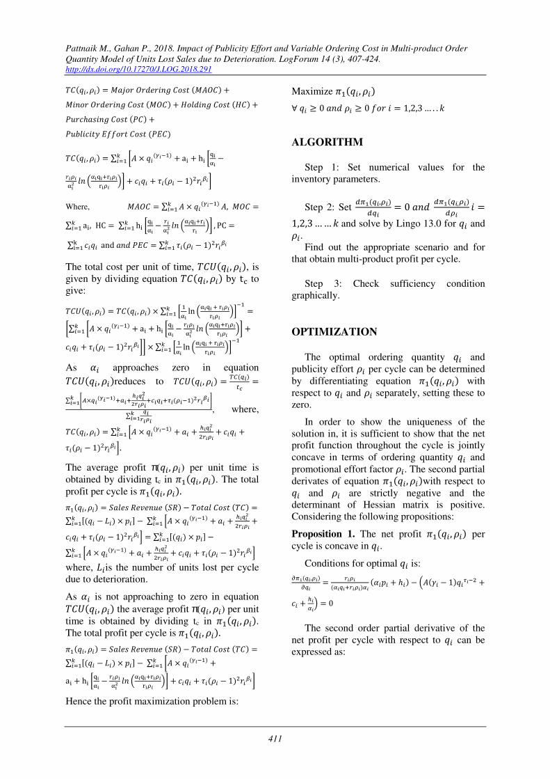
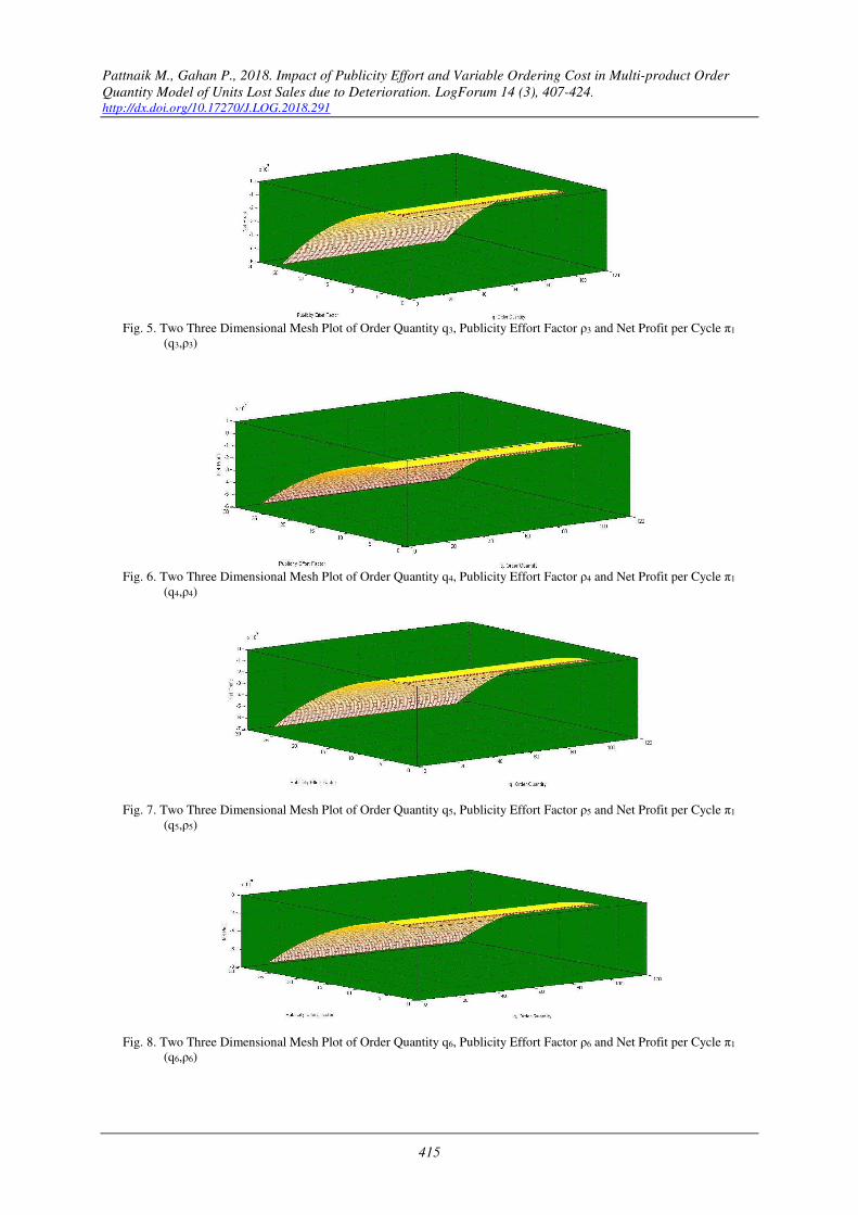
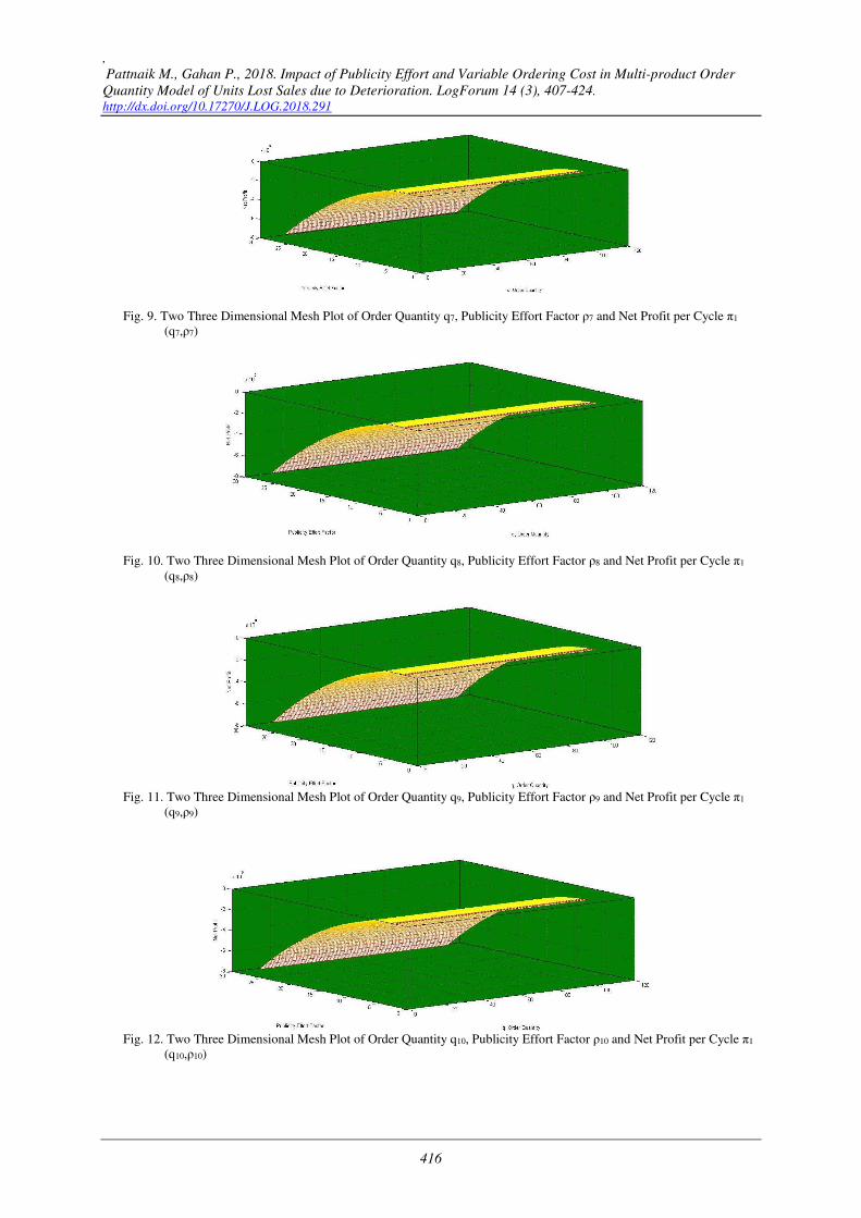
Fig. 1 represents the relationship between

the order quantity �� and fuctional major

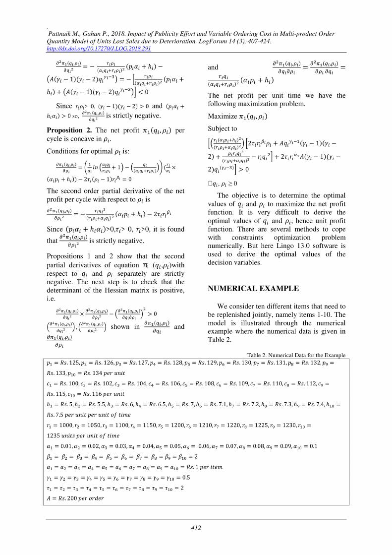
ordering cost MAOC. Fig. 2 shows the

relationship between the order quantity �� and

units lost per cycle due to deterioration J�, Fig.

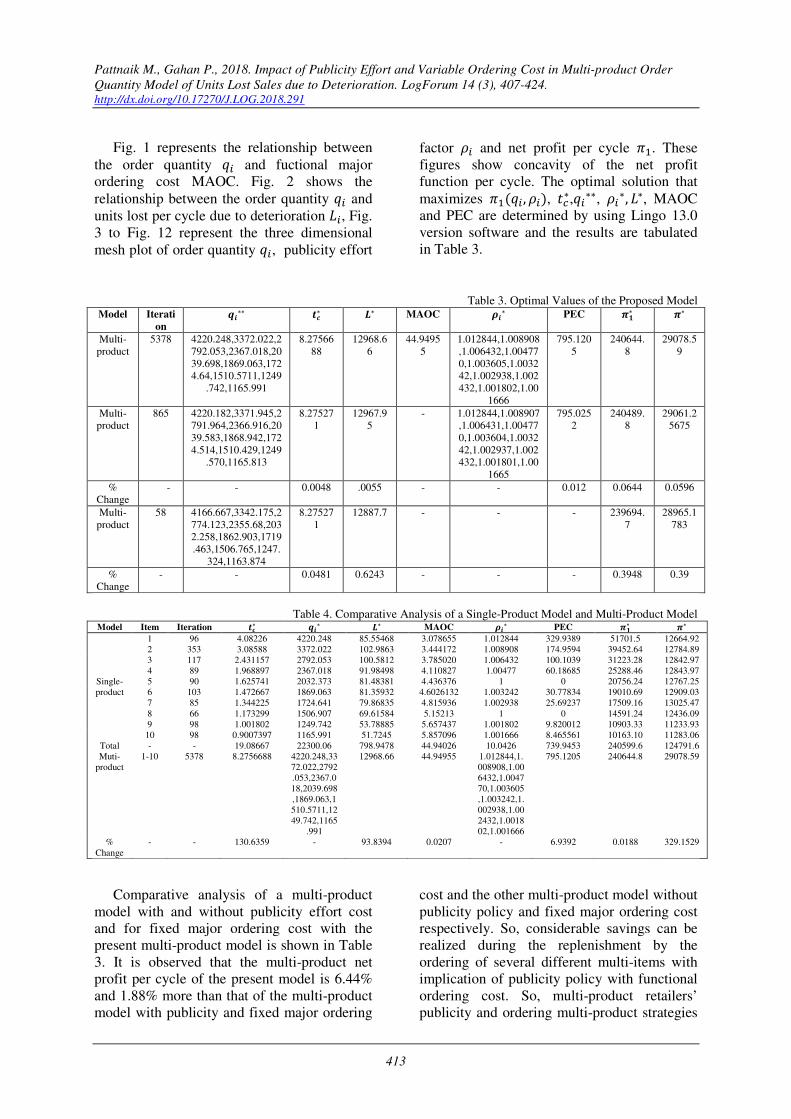
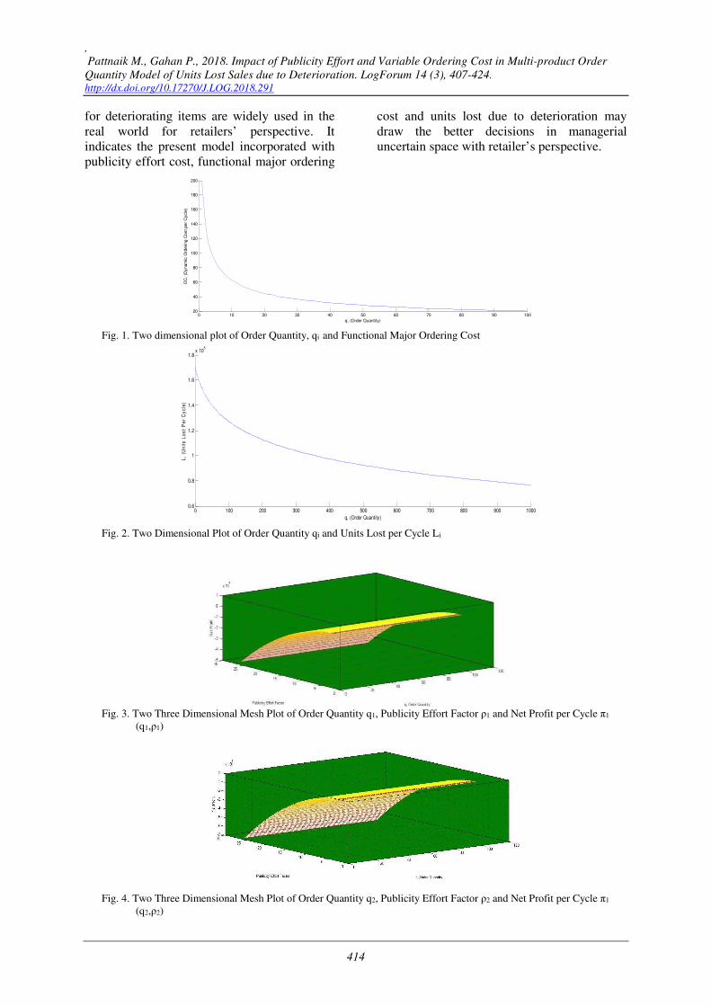
3 to Fig. 12 represent the three dimensional

mesh plot of order quantity ��, publicity effort

factor �� and net profit per cycle )�. These

figures show concavity of the net profit

function per cycle. The optimal solution that

maximizes )�(��, ��), ��∗,��∗∗, ��∗, J∗, MAOC

and PEC are determined by using Lingo 13.0

version software and the results are tabulated

in Table 3.

Table 3. Optimal Values of the Proposed Model

Model Iteration

¡∗∗ ¢£∗ ¤∗ MAOC ¥¡∗ PEC ¦§∗ ¦∗

Multi-

product

5378 4220.248,3372.022,2

792.053,2367.018,20

39.698,1869.063,172

4.64,1510.5711,1249

.742,1165.991

8.27566

88

12968.6

6

44.9495

5

1.012844,1.008908

,1.006432,1.00477

0,1.003605,1.0032

42,1.002938,1.002

432,1.001802,1.00

1666

795.120

5

240644.

8

29078.5

9

Multi-

product

865 4220.182,3371.945,2

791.964,2366.916,20

39.583,1868.942,172

4.514,1510.429,1249

.570,1165.813

8.27527

1

12967.9

5

- 1.012844,1.008907

,1.006431,1.00477

0,1.003604,1.0032

42,1.002937,1.002

432,1.001801,1.00

1665

795.025

2

240489.

8

29061.2

5675

%

Change

- - 0.0048 .0055 - - 0.012 0.0644 0.0596

Multi-

product

58 4166.667,3342.175,2

774.123,2355.68,203

2.258,1862.903,1719

.463,1506.765,1247.

324,1163.874

8.27527

1

12887.7 - - - 239694.

7

28965.1

783

%

Change

- - 0.0481 0.6243 - - - 0.3948 0.39

Table 4. Comparative Analysis of a Single-Product Model and Multi-Product Model Model Item Iteration ¢£∗ ¡∗ ¤∗ MAOC ¥¡∗ PEC ¦§∗ ¦∗

Single-

product

1 96 4.08226 4220.248 85.55468 3.078655 1.012844 329.9389 51701.5 12664.92

2 353 3.08588 3372.022 102.9863 3.444172 1.008908 174.9594 39452.64 12784.89

3 117 2.431157 2792.053 100.5812 3.785020 1.006432 100.1039 31223.28 12842.97

4 89 1.968897 2367.018 91.98498 4.110827 1.00477 60.18685 25288.46 12843.97

5 90 1.625741 2032.373 81.48381 4.436376 1 0 20756.24 12767.25

6 103 1.472667 1869.063 81.35932 4.6026132 1.003242 30.77834 19010.69 12909.03

7 85 1.344225 1724.641 79.86835 4.815936 1.002938 25.69237 17509.16 13025.47

8 66 1.173299 1506.907 69.61584 5.15213 1 0 14591.24 12436.09

9 98 1.001802 1249.742 53.78885 5.657437 1.001802 9.820012 10903.33 11233.93

10 98 0.9007397 1165.991 51.7245 5.857096 1.001666 8.465561 10163.10 11283.06

Total - - 19.08667 22300.06 798.9478 44.94026 10.0426 739.9453 240599.6 124791.6

Muti-

product

1-10 5378 8.2756688 4220.248,33

72.022,2792

.053,2367.0

18,2039.698

,1869.063,1

510.5711,12

49.742,1165

.991

12968.66 44.94955 1.012844,1.

008908,1.00

6432,1.0047

70,1.003605

,1.003242,1.

002938,1.00

2432,1.0018

02,1.001666

795.1205 240644.8 29078.59

%

Change

- - 130.6359 - 93.8394 0.0207 - 6.9392 0.0188 329.1529

Comparative analysis of a multi-product

model with and without publicity effort cost

and for fixed major ordering cost with the

present multi-product model is shown in Table

3. It is observed that the multi-product net

profit per cycle of the present model is 6.44%

and 1.88% more than that of the multi-product

model with publicity and fixed major ordering

cost and the other multi-product model without

publicity policy and fixed major ordering cost

respectively. So, considerable savings can be

realized during the replenishment by the

ordering of several different multi-items with

implication of publicity policy with functional

ordering cost. So, multi-product retailers’

publicity and ordering multi-product strategies

,




414

for deteriorating items are widely used in the

real world for retailers’ perspective. It

indicates the present model incorporated with

publicity effort cost, functional major ordering

cost and units lost due to deterioration may

draw the better decisions in managerial

uncertain space with retailer’s perspective.

Fig. 1. Two dimensional plot of Order Quantity, qi and Functional Major Ordering Cost

Fig. 2. Two Dimensional Plot of Order Quantity qi and Units Lost per Cycle Li

Fig. 3. Two Three Dimensional Mesh Plot of Order Quantity q1, Publicity Effort Factor ρ1 and Net Profit per Cycle π1

(q1,ρ1)


(q2,ρ2)

0 10 20 30 40 50 60 70 80 90 10020

40

60

80

100

120

140

160

180

200

q, (Order Quantity)

OC

, (D

ynam

ic O

rdering C

ost

per

Cycle

)

0 100 200 300 400 500 600 700 800 900 10000.6

0.8

1

1.2

1.4

1.6

1.8x 10

5

q, (Order Quantity)

L,

(Un

its

Lo

st

Pe

r C

yc

le)




415


(q3,ρ3)


(q4,ρ4)


(q5,ρ5)


(q6,ρ6)

,




416


(q7,ρ7)


(q8,ρ8)


(q9,ρ9)


(q10,ρ10)




417

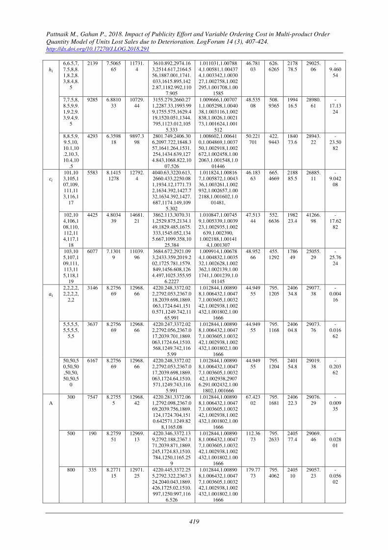
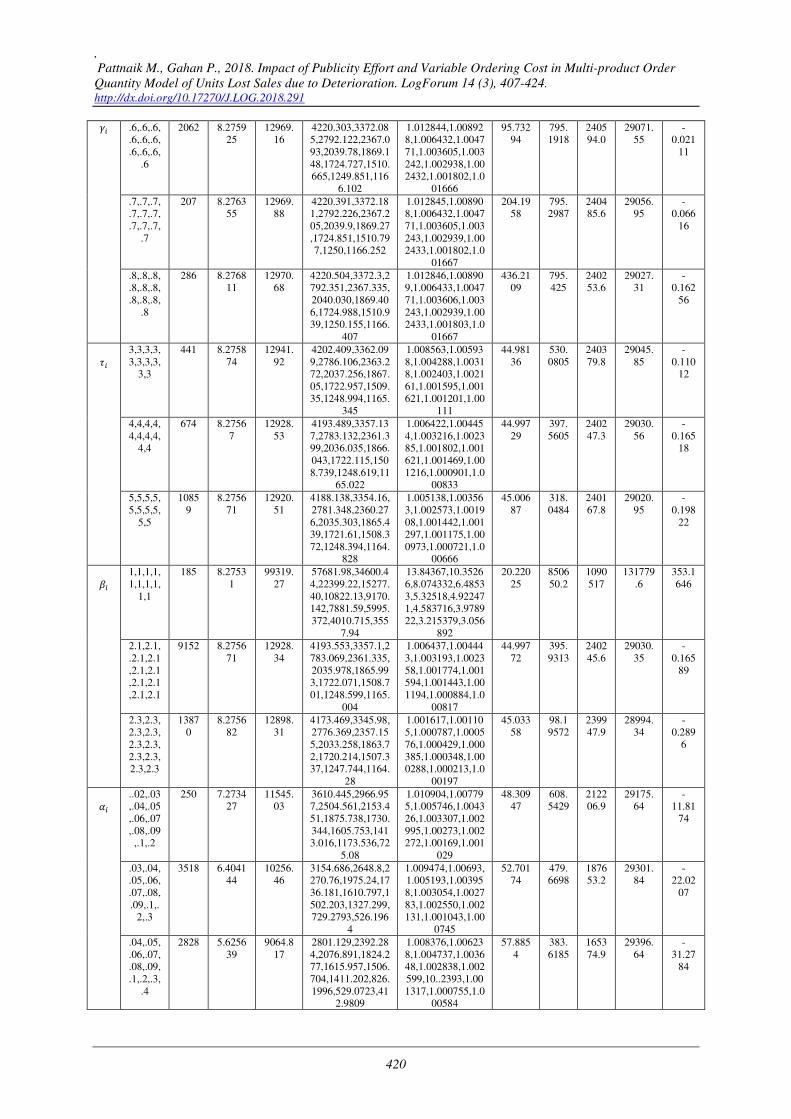
SENSITIVITY ANALYSIS

It is interesting to investigate the

influence of the major inventory parameters, �,��, ℎ� , ��, (� , ", '�, �� , ��(N2 !�on retailers’

perspective multi-product order quantity

model. The computational results shown in

Table 5 indicate the following managerial

phenomena:

• ��, � = 1,2, … 10 order quantities, �� the

cycle length, L total units lost due to

deterioration and �� the publicity effort

factor are highly sensitive, MAOC

functional major ordering cost is sensitive,

PEC publicity effort cost per cycle is

highly sensitive, )� the net profit per cycle

and ) the average profit per cycle are

highly sensitive to the parameter � selling

price for item i.

• ��, � = 1,2, … 10 order quantities are

sensitive, �� the cycle length is insensitive

L total units lost due to deterioration is

sensitive, �� the publicity effort factor are

insensitive, MAOC functional major

ordering cost is moderately sensitive, PEC

publicity effort cost per cycle is

insensitive, )� the net profit per cycle and ) the average profit per cycle are sensitive

to the parameter ��the consumption rate for

item i.

• ��, � = 1,2, … 10 order quantities and ��

the cycle length, L total units lost due to

deterioration is sensitive, �� the publicity

effort factor are insensitive, MAOC

functional major ordering cost, PEC

publicity effort cost per cycle and )� the

net profit per cycle are sensitive and ) the

average profit per cycle is moderately

sensitive to the parameter ℎ�holding cost

of item i per unit per unit of time.



deterioration, �� the publicity effort factor,

MAOC functional major ordering cost,

PEC publicity effort cost per cycle, )� the

net profit per cycle and ) the average

profit per cycle are sensitive to the

parameter �� purchasing cost for item i.


insensitive, �� the cycle length, L total

units lost due to deterioration, �� the

publicity effort factor, MAOC functional

major ordering cost, PEC publicity effort

cost per cycle are insensitive, )� the net

profit per cycle and ) the average profit

per cycle is moderately sensitive to the

parameter (� minor ordering cost of item i.



deterioration, �� the publicity effort factor

are insensitive, MAOC functional major

ordering cost is highly sensitive, PEC

publicity effort cost per cycle is

insensitive, )� the net profit per cycleand ) the average profit per cycle are

moderately sensitive to the parameter A

major ordering cost per order.

• ��, � = 1,2, … 10 order quantities and ��

the cycle length are insensitive, L total

units lost due to deterioration is

moderately sensitive, �� the publicity effort

factor is insensitive, MAOC functional

major ordering cost is highly sensitive,

PEC publicity effort cost per cycle is

insensitive, )� the net profit per cycle and ) the average profit per cycle is

moderately sensitive to the parameter '� of

the publicity effort cost per cycle.


sensitive, �� the cycle length, L total units

lost due to deterioration, �� the publicity

effort factor are insensitive, MAOC

functional major ordering cost is

moderately sensitive, PEC publicity effort

cost per cycle is highly sensitive, )� the

net profit per cycle and ) the average

profit per cycle are moderately sensitive to

the parameter �� of the publicity effort cost

per cycle.


highly sensitive, �� the cycle length is

insensitive, L total units lost due to

deterioration is highly sensitive, �� the

publicity effort factor, MAOC functional

major ordering cost, PEC publicity effort

cost per cycle, )� the net profit per cycle

and ) the average profit per cycle are

highly sensitive to the parameter �� of the

publicity effort cost per cycle.


sensitive, �� the cycle length, L total units

,




418

lost due to deterioration are sensitive, �� the publicity effort factor are insensitive,

MAOC functional major ordering cost and

PEC publicity effort cost per cycle are

sensitive, )� the net profit per cycle is

highly sensitive and ) the average profit

per cycle is moderately sensitive to the

parameter !� of the percentage of units lost

due to deterioration.

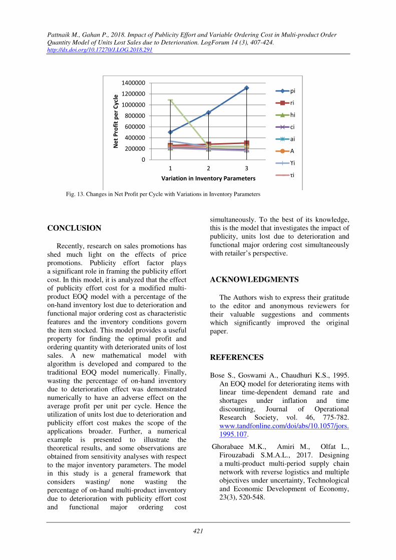
Fig. 13 is about net profit per cycle

variations with respect to inventory

parameters. The profit increases slightly with

increase in per unit selling price, consumption

rate and one parameter of publicity effort cost

and then decreasing and the profit increases

slightly with increase in consumption rate. The

profit decreases with increase in holding cost

per unit per unit time, purchasing cost per unit

for item i and the profit decreases slightly with

increase in one parameter of publicity effort

cost, minor ordering cost, parameter of

functional major ordering cost, MAOC and

percentage of units lost due to deterioration

respectively. This suggests that the retailer

should work on the holding cost per unit per

unit of time, purchasing cost per unit, minor

ordering cost, parameters of publicity cost

function, functional major ordering cost and

percentage of units lost due to deterioration for

item i. The retailer should put large order with

implementing publicity strategy and

implementation of appropriate preservation

technology to save in ordering cost and

wastage cost as a result profit of retailers can

be increased significantly.

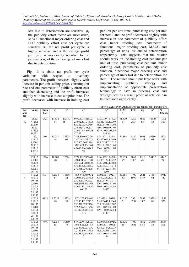
Table 4. Sensitivity Analyses of the Significant Parameters Parameter

Value Iteration

¢£∗ ¤∗ ¡∗ ¥¡∗ MAOC

PEC ¦§∗ ¦∗ % Change

�

126,12

7,128,1

29,130,

131,13

2,133,1

34,135

6323 11.832

94

19218.

46

5979.433,4818.72

2,4032.471,3460.6

82,3023.335,2769.

234,2554.343,227

2.408,1948.699,18

17.747

1.025039,1.01372

7,1.013103,1.0099

75,1.007756,1.006

969,1.006309,1.00

5389,1.004291,1.0

03966

36.829

14

3250

.313

5032

65

42530.

85

109.1

319

127,

128,12

9,130,1

31,132,

133,13

4,135,1

36

301 15.281

44

25725.

07

7808.809,6307.79,

5300.66,4573.65,4

020.962,3680.894,

3393.627,3042.03

4,2653.794,2474.7

98

1.041171,1.02944

3,1.022024,1.0169

89,1.013402,1.012

029,1.010882,1.00

3546,1.00201,1.00

0231

31.898

42

9140

.703

8601

31.6

56286.

03

257.4

279

128,12

9,130,1

31,132,

133,13

4,135,1

36,137

1206 18.605

28

32514.

9

9727.495,7850697

,6604.34,5711.394

,5036.643,4607.34

9,4245.226,3821.7

27,3366.939,3138.

779

1.061179,1.04398

7,1.033127,1.0257

53,1.02049,1.0183

72,1.016607,1.014

541,1.012235,1.01

1299

28.478

49

2065

7.67

1310

622

7443.5

5

444.6

293

�� 1100,1

150,12

00,125

0,1300,

1310,1

320,13

25,133

0,1335

3031 8.2930

54

14116.

24

4636.911,3690.32

1,3044.242,2571.8

55,2209.049,2023.

018,1865.575,163

3.567,1351.144,12

60.225

1.002995,1.00271

5,1.002249,1.0016

66,1.001541,1.011

676,1.008133,1.00

5896,1.004389,1.0

03327

43.153

52

795.

1090

2621

81.9

31614.

64

8.949

747

1200,1

250,13

00,135

0,1400,

1410,1

420,14

25,143

0,1435

4715 8.2755

88

15263.

37

5053.575,4008.62

1,3296.432,2776.6

93,2378.399,2176.

972,2006.51,1756.

563,1452.547,135

4.46

1.010703,1.00748

2,1.005442,1.0040

63,1.003090,1.002

782,1.002524,1.00

2091,1.001549,1.0

01434

41.557

51

795.

0998

2837

18.7

34283.

81

17.89

937

1300,1

350,14

00,145

0,1500,

1510,1

520,15

25,153

0,1535

7646 8.2755

55

16410.

73

5470.239,4326.92,

3548.622,2981.53

2,2547.75,2330.92

7,2147.446,1879.5

6,1553.95,1448.69

5

1.00988,1.006928,

1.005053,1.00378

3,1.002884,1.0025

98,1.002358,1.001

954,1.001448,1.00

134

40.126

85

795.

0921

3052

55.3

36886.

38

26.84

891




419

ℎ� 6,6.5,7,

7.5,8,8.

1,8.2,8.

3,8.4,8.

5

2139 7.5065

65

11731.

4

3610.892,2974.16

3,2514.617,2164.5

56,1887.001,1741.

033,1615.895,142

2.87,1182.992,110

7.905

1.011031,1.00788

4,1.00581,1.00437

4,1.003342,1.0030

27,1.002758,1.002

295,1.001708,1.00

1585

46.781

03

626.

6265

2178

78.5

29025.

06

-

9.460

54

7,7.5,8,

8.5,9,9.

1,9.2,9.

3,9.4,9.

5

9285 6.8810

33

10729.

44

3155.279,2660.27

1,2287.33,1993.99

9,1755.575,1629.4

19,1520.051,1344.

795,1123.012,105

5.333

1.009666,1.00707

1,1.005298,1.0040

38,1.003116,1.002

838,1.0026,1.0021

73,1.001624,1.001

512

48.535

08

508.

9365

1994

16.5

28980.

61

-

17.13

24

8,8.5,9,

9.5,10,

10.1,10

.2,10.3,

10.4,10

.5

4293 6.3598

18

9897.3

98

2801.749,2406.30

6,2097.722,1848.3

57,1641.264,1531.

254,1434.639,127

4.843,1068.822,10

07.526

1.008602,1.00641

0,1.004869,1.0037

50,1.002918,1.002

672,1.002458,1.00

2063,1.001548,1.0

01446

50.221

701

422.

9443

1840

73.6

28943.

22

-

23.50

82

�� 101,10

3,105,1

07,109,

111,11

3,116,1

17

5583 8.1415

1278

12792.

4

4040.63,3220.613,

2660.433,2250.08

1,1934.12,1771.73

2,1634.392,1427.7

32,1634.392,1427.

687,1174.149,109

5.302

1.011824,1.00816

7,1.005872,1.0043

36,1.003261,1.002

932,1.002657,1.00

2188,1.001602,1.0

01481,

46.183

63

665.

4669

2188

85.5

26885.

11

-

9.042

08

102,10

4,106,1

08,110,

112,11

4,117,1

18

4425 4.8034

39

14681.

21

3862.113,3070.31

1,2529.875,2134.1

49,1829.485,1675.

333,1545.052,134

5.667,1099.358,10

25.384

1.010847,1.00745

9,1.005339,1.0039

23,1.002935,1.002

639,1.002390,

1.002188,1.00141

4,1.001307

47.513

44

552.

6636

1982

23.4

41266.

98

-

17.62

82

103,10

5,107,1

09,111,

113,11

5,118,1

19

6077 7.1301

9

11039.

96

3684.672,2921.09

3,2433.359,2019.2

02,1725.781,1579.

849,1456.608,126

4.497,1025.355,95

6.2227

1.009914,1.00678

4,1.004832,1.0035

32,1.002628,1.002

362,1.002139,1.00

1741,1.001239,1.0

01145

48.952

66

455.

1292

1786

49

25055.

29

-

25.76

24

(� 2,2,2,2,

2,2,2,2,

2,2

3146 8.2756

69

12968.

66

4220.248,3372.02

2,2792.053,2367.0

18,2039.698,1869.

063,1724.641,151

0.571,1249.742,11

65.991

1.012844,1.00890

8,1.006432,1.0047

7,1.003605,1.0032

42,1.002938,1.002

432,1.001802,1.00

1666

44.949

55

795.

1205

2406

34.8

29077.

38

-

0.004

16

5,5,5,5,

5,5,5,5,

5,5

3637 8.2756

69

12968.

66

4220.247,3372.02

2,2792.056,2367.0

17,2039.701,1869.

063,1724.64,1510.

568,1249.742,116

5.99

1.012844,1.00890

8,1.006432,1.0047

7,1.003605,1.0032

42,1.002938,1.002

432,1.001802,1.00

1666

44.949

55

795.

1168

2406

04.8

29073.

76

-

0.016

62

50,50,5

0,50,50

,50,50,

50,50,5

0

6167 8.2756

69

12968.

66

4220.248,3372.02

2,2792.053,2367.0

17,2039.698,1869.

063,1724.64,1510.

571,1249.743,116

5.991

1.012844,1.00890

8,1.006432,1.0047

7,1.003605,1.0032

42,1.002938,2907

6.291.002432,1.00

1802,1.001666

44.949

55

795.

1204

2401

54.8

29019.

38

-

0.203

62

A

300 7547 8.2755

5

12968.

42

4220.281,3372.06

1,2792.098,2367.0

69,2039.756,1869.

124,1724.704,151

0.642571,1249.82

8,1165.08

1.012844,1.00890

8,1.006432,1.0047

7,1.003605,1.0032

42,1.002938,1.002

432,1.001802,1.00

1666

67.423

02

795.

1681

2406

22.3

29076.

29

-

0.009

35

500 190 8.2759

51

12969.

13

4220.346,3372.13

9,2792.188,2367.1

71,2039.871,1869.

245,1724.83,1510.

784,1250,1165.25

9

1.012844,1.00890

8,1.006432,1.0047

7,1.003605,1.0032

42,1.002938,1.002

432,1.001802,1.00

1666

112.36

73

795.

2633

2405

77.4

29069.

46

-

0.028

01

800 335 8.2771

15

12971.

25

4220.445,3372.25

5,2792.322,2367.3

24,2040.043,1869.

426,1725.02,1510.

997,1250.997,116

6.526

1.012844,1.00890

8,1.006432,1.0047

7,1.003605,1.0032

42,1.002938,1.002

432,1.001802,1.00

1666

179.77

73

795.

4062

2405

10

29057.

23

-

0.056

02

,




420

'� .6,.6,.6,

.6,.6,.6,

.6,.6,.6,

.6

2062 8.2759

25

12969.

16

4220.303,3372.08

5,2792.122,2367.0

93,2039.78,1869.1

48,1724.727,1510.

665,1249.851,116

6.102

1.012844,1.00892

8,1.006432,1.0047

71,1.003605,1.003

242,1.002938,1.00

2432,1.001802,1.0

01666

95.732

94

795.

1918

2405

94.0

29071.

55

-

0.021

11

.7,.7,.7,

.7,.7,.7,

.7,.7,.7,

.7

207 8.2763

55

12969.

88

4220.391,3372.18

1,2792.226,2367.2

05,2039.9,1869.27

,1724.851,1510.79

7,1250,1166.252

1.012845,1.00890

8,1.006432,1.0047

71,1.003605,1.003

243,1.002939,1.00

2433,1.001802,1.0

01667

204.19

58

795.

2987

2404

85.6

29056.

95

-

0.066

16

.8,.8,.8,

.8,.8,.8,

.8,.8,.8,

.8

286 8.2768

11

12970.

68

4220.504,3372.3,2

792.351,2367.335,

2040.030,1869.40

6,1724.988,1510.9

39,1250.155,1166.

407

1.012846,1.00890

9,1.006433,1.0047

71,1.003606,1.003

243,1.002939,1.00

2433,1.001803,1.0

01667

436.21

09

795.

425

2402

53.6

29027.

31

-

0.162

56

�� 3,3,3,3,

3,3,3,3,

3,3

441 8.2758

74

12941.

92

4202.409,3362.09

9,2786.106,2363.2

72,2037.256,1867.

05,1722.957,1509.

35,1248.994,1165.

345

1.008563,1.00593

8,1.004288,1.0031

8,1.002403,1.0021

61,1.001595,1.001

621,1.001201,1.00

111

44.981

36

530.

0805

2403

79.8

29045.

85

-

0.110

12

4,4,4,4,

4,4,4,4,

4,4

674 8.2756

7

12928.

53

4193.489,3357.13

7,2783.132,2361.3

99,2036.035,1866.

043,1722.115,150

8.739,1248.619,11

65.022

1.006422,1.00445

4,1.003216,1.0023

85,1.001802,1.001

621,1.001469,1.00

1216,1.000901,1.0

00833

44.997

29

397.

5605

2402

47.3

29030.

56

-

0.165

18

5,5,5,5,

5,5,5,5,

5,5

1085

9

8.2756

71

12920.

51

4188.138,3354.16,

2781.348,2360.27

6,2035.303,1865.4

39,1721.61,1508.3

72,1248.394,1164.

828

1.005138,1.00356

3,1.002573,1.0019

08,1.001442,1.001

297,1.001175,1.00

0973,1.000721,1.0

00666

45.006

87

318.

0484

2401

67.8

29020.

95

-

0.198

22

�� 1,1,1,1,

1,1,1,1,

1,1

185 8.2753

1

99319.

27

57681.98,34600.4

4,22399.22,15277.

40,10822.13,9170.

142,7881.59,5995.

372,4010.715,355

7.94

13.84367,10.3526

6,8.074332,6.4853

3,5.32518,4.92247

1,4.583716,3.9789

22,3.215379,3.056

892

20.220

25

8506

50.2

1090

517

131779

.6

353.1

646

2.1,2.1,

.2.1,2.1

,2.1,2.1

,2.1,2.1

,2.1,2.1

9152 8.2756

71

12928.

34

4193.553,3357.1,2

783.069,2361.335,

2035.978,1865.99

3,1722.071,1508.7

01,1248.599,1165.

004

1.006437,1.00444

3,1.003193,1.0023

58,1.001774,1.001

594,1.001443,1.00

1194,1.000884,1.0

00817

44.997

72

395.

9313

2402

45.6

29030.

35

-

0.165

89

2.3,2.3,

2.3,2.3,

2.3,2.3,

2.3,2.3,

2.3,2.3

1387

0

8.2756

82

12898.

31

4173.469,3345.98,

2776.369,2357.15

5,2033.258,1863.7

2,1720.214,1507.3

37,1247.744,1164.

28

1.001617,1.00110

5,1.000787,1.0005

76,1.000429,1.000

385,1.000348,1.00

0288,1.000213,1.0

00197

45.033

58

98.1

9572

2399

47.9

28994.

34

-

0.289

6

!� ..02,.03

,.04,.05

,.06,.07

,.08,.09

,.1,.2

250 7.2734

27

11545.

03

3610.445,2966.95

7,2504.561,2153.4

51,1875.738,1730.

344,1605.753,141

3.016,1173.536,72

5.08

1.010904,1.00779

5,1.005746,1.0043

26,1.003307,1.002

995,1.00273,1.002

272,1.00169,1.001

029

48.309

47

608.

5429

2122

06.9

29175.

64

-

11.81

74

.03,.04,

.05,.06,

.07,.08,

.09,.1,.

2,.3

3518 6.4041

44

10256.

46

3154.686,2648.8,2

270.76,1975.24,17

36.181,1610.797,1

502.203,1327.299,

729.2793,526.196

4

1.009474,1.00693,

1.005193,1.00395

8,1.003054,1.0027

83,1.002550,1.002

131,1.001043,1.00

0745

52.701

74

479.

6698

1876

53.2

29301.

84

-

22.02

07

.04,.05,

.06,.07,

.08,.09,

.1,.2,.3,

.4

2828 5.6256

39

9064.8

17

2801.129,2392.28

4,2076.891,1824.2

77,1615.957,1506.

704,1411.202,826.

1996,529.0723,41

2.9809

1.008376,1.00623

8,1.004737,1.0036

48,1.002838,1.002

599,10..2393,1.00

1317,1.000755,1.0

00584

57.885

4

383.

6185

1653

74.9

29396.

64

-

31.27

84




421

Fig. 13. Changes in Net Profit per Cycle with Variations in Inventory Parameters

CONCLUSION

Recently, research on sales promotions has

shed much light on the effects of price

promotions. Publicity effort factor plays

a significant role in framing the publicity effort

cost. In this model, it is analyzed that the effect

of publicity effort cost for a modified multi-

product EOQ model with a percentage of the

on-hand inventory lost due to deterioration and

functional major ordering cost as characteristic

features and the inventory conditions govern

the item stocked. This model provides a useful

property for finding the optimal profit and

ordering quantity with deteriorated units of lost

sales. A new mathematical model with

algorithm is developed and compared to the

traditional EOQ model numerically. Finally,

wasting the percentage of on-hand inventory

due to deterioration effect was demonstrated

numerically to have an adverse effect on the

average profit per unit per cycle. Hence the

utilization of units lost due to deterioration and

publicity effort cost makes the scope of the

applications broader. Further, a numerical

example is presented to illustrate the

theoretical results, and some observations are

obtained from sensitivity analyses with respect

to the major inventory parameters. The model

in this study is a general framework that

considers wasting/ none wasting the

percentage of on-hand multi-product inventory

due to deterioration with publicity effort cost

and functional major ordering cost

simultaneously. To the best of its knowledge,

this is the model that investigates the impact of

publicity, units lost due to deterioration and

functional major ordering cost simultaneously

with retailer’s perspective.

ACKNOWLEDGMENTS

The Authors wish to express their gratitude

to the editor and anonymous reviewers for

their valuable suggestions and comments

which significantly improved the original

paper.

REFERENCES

Bose S., Goswami A., Chaudhuri K.S., 1995.

An EOQ model for deteriorating items with

linear time-dependent demand rate and

shortages under inflation and time

discounting, Journal of Operational

Research Society, vol. 46, 775-782.

www.tandfonline.com/doi/abs/10.1057/jors.

1995.107.

Ghorabaee M.K., Amiri M., Olfat L.,

Firouzabadi S.M.A.L., 2017. Designing

a multi-product multi-period supply chain

network with reverse logistics and multiple

objectives under uncertainty, Technological

and Economic Development of Economy,

23(3), 520-548.

0

200000

400000

600000

800000

1000000

1200000

1400000

1 2 3

Ne

t P

rofi

t p

er

Cy

cle

Variation in Inventory Parameters

pi

ri

hi

ci

ai

A

ϒi

τi

,




422

http://dx.doi.org/10.3846/20294913.2017.1

312630.

Goyal S.K., Gunasekaran A., 1995. An

integrated production-inventory-marketing

model for deteriorating items, Computers

and Industrial Engineering, 28, 755-762.

http://dx.doi.org/10.1016/0360-

8352(95)00016-T

Gupta D., Gerchak Y., 1995. Joint product

durability and lot sizing models, European

Journal of Operational Research, 84, 371-

384.

http://dx.doi.org/10.1016/0377-

2217(93)E0273-Z

Hammer M., 2001. The superefficient

company, Harvard Business Review, vol.

79, 82-91.

https://hbr.org/2001/09/the-superefficient-

company.

Hariga M., 1994. Economic analysis of

dynamic inventory models with non-

stationary costs and demand, International

Journal of Production Economics, 36, 255-

266.

https://doi.org/10.1016/0925-

5273(94)00039-5

Hariga M., 1995. An EOQ model for

deteriorating items with shortages and time-

varying demand, Journal of Operational

Research Society, 46, 398-404.

http://dx.doi.org/10.1057/jors.1995.54

Hariga M., 1996, Optimal EOQ models for

deteriorating items with time-varying

demand, Journal of Operational Research

Society, 47, 1228-1246.

http://dx.doi.org/10.1016/0925-

5273(94)00039-5

Jain K., Silver E., 1994. A lot sizing for

a product subject to obsolescence or

perishability, European Journal of

Operational Research, 75, 287-295.

http://dx.doi.org/10.1016/0377-

2217(94)90075-2

Karimi R., Ghezavati V.R., Damghani K.K.,

2015. Optimization of multi-product, multi-

period closed loop supply chain under

uncertainty in product return rate: case

study in Kalleh dairy company, Journal of

Industrial and Systems Engineering, 8(3),

95-114.

http://www.jise.ir/article_10151.html.

Mishra V.K., 2012. Inventory model for time

dependent holding cost and deterioration

with salvage value and shortages, The

Journal of Mathematics and Computer

Science, 4(1), 37-47. www.isr-

publications.com/.../download-inventory-

model-for-time-dependent-holding.

Padmanabhan G., Vrat P., 1995. EOQ models

for perishable items under stock dependent

selling rate, European Journal of

Operational Research, 86, 281-292.

http://dx.doi.org/10.1016/0377-

2217(94)00103-J

Pattnaik M., 2011. A note on non linear

optimal inventory policy involving instant

deterioration of perishable items with price

discounts, The Journal of Mathematics and

Computer Science, 3(2), 145-155. www.isr-

publications.com/.../download-a-note-on-

non-linear-optimal-inventory-polic.. .

Pattnaik M., 2012. Models of Inventory

Control, Lambart Academic Publishing

Company, Germany.

Pattnaik M., 2012. An EOQ model for

perishable items with constant demand and

instant Deterioration, Decision, vol. 39(1),

55-61. www.sciepub.com/reference/77772.

Roy T.K., Maiti M., 1997. A Fuzzy EOQ

model with demand dependent unit cost

under limited storage capacity, European

Journal of Operational Research, 99, 425 –

432.

http://dx.doi.org/10.1016/S0377-

2217(96)00163-4

Salameh M.K., Jaber M.Y., Noueihed, N.,

1993. Effect of deteriorating items on the

instantaneous replenishment model,

Production Planning and Control, 10(2),

175-180.

http://dx.doi.org/10.1080/09537289923332

5

Sana S.S., 2015. An EOQ model for stochastic

demand for limited capacity of own

warehouse. Ann Oper Res, 233, 1, 383–

399.

http://dx.doi.org/10.1007/s10479-013-1510-

5




423

Tabatabaei M.S.R., Sadjadi S.J., Makui A.

2017. Optimal pricing and marketing

planning for deteriorating items. PLoS

ONE 12(3): e0172758.

http://dx.doi.org/10.1371/journal.pone.0172

758

Tsao Y.C., Sheen G.J., 2008. Dynamic pricing,

promotion and replenishment policies for

a deteriorating item under permissible delay

in payment, Computers and Operations

Research, 35, 3562-3580.

www.sciepub.com/reference/77782.

Tsao Y.C., Sheen G.J., 2012, A multi-item

supply chain with credit periods and weight

freight cost discounts, International Journal

of Production Economics, 135, 106-115.

http://dx.doi.org/10.1016/j.ijpe.2010.11.013

WPŁYW WYDATKÓW I ZMIENNYCH KOSZTÓW W MODELU ZAMAWIANIA WIELO-ASORTYMENTOWYM NA STRATY SPRZEDAŻY W WYNIKU NISZCZENIA

STRESZCZENIE. Wstęp: W pracy poddano analizie model ekonomicznej wielkości partii dla zamówień wielo-

asortymentowych poprzez alokację procentu jednostek utraconych w wyniku zniszczenia oraz poprzez inwentaryzację

przy uwzględnieniu inwestycji w promocję oraz koszty zamówień. Celem pracy było maksymalizacji zysku netto

poprzez odpowiednie kształtowanie wielkości zamówienia, długości cyklu odtworzeniowego oraz ilości jednostek,

ulegających zniszczeniu.

Metody: Opracowany matematyczny algorytm w celu znalezienia ważnych charakterystyk wklęsłości funkcji zysku

netto. Zaprezentowany przykłady w celu zilustrowania wyników uzyskanych przy zastosowaniu opracowanego modelu

oraz jego zalet. Na końcu przeprowadzono analizę wrażliwości zysku netto dla głównych parametrów

inwentaryzacyjnych.

Wyniki i wnioski: Proponowany model stanowi ogólny schemat uwzględniający utratę procentową zapasów w wyniku

zniszczenia przy uwzględnieniu zmiennych kosztów związanych z zamawianiem towarów.

Słowa kluczowe: wieloasortymentowość, zmienny koszt zamówienia, zniszczenie, maksymalizacja zysków.

EINFLUSS VON AUSGABEN UND VARIABLEN KOSTEN IM MEHRSORTIMENT-BESTELLUNGSMODELL AUF VERLUSTE BEI VERKAUF INFOLGE EINES VERDERBS

ZUSAMMENFASSUNG. Einleitung: Im Rahmen der vorliegenden Arbeit wurde das Modell einer wirtschaftlichen

Losgröße für die Mehrsortiment-Bestellung anhand einer Allokation des Prozentsatzes von verlorengegangenen

Einheiten infolge eines Verderbs und mithilfe einer Inventarisierung bei Berücksichtigung von Investitionen in die

Promotion und Bestellungskosten analysiert. Das Ziel der Arbeit war es, den Netto-Gewinn durch eine entsprechende

Gestaltung von Bestellungsgrößen, ferner von der Dauer des Wiederbeschaffungszyklus und der Anzahl von den einem

Verderb unterliegenden Einheiten zu maximieren.

Methoden: Als die brauchbare Methode dafür gilt der ausgearbeitete mathematische Algorithmus zwecks der Ermittlung

von relevanten Charakteristika der Höhlung der Funktion vom Netto-Gewinn. Ferner das dargestellte Beispiel für die

Projizierung der unter Anwendung des ausgearbeiteten Modells gewonnenen Ergebnissen und dessen Vorteile. Zum

Ausgang der Forschung wurde eine Analyse der Empfindlichkeit des Netto-Gewinns für die grundlegenden

Inventarisierungsparameter durchgeführt.

,




424

Ergebnisse und Fazit: Das unterbreitete Modell gilt als ein allgemeines Schema, das einen prozentuellen Verlust von

Vorräten infolge eines Verderbs bei der Berücksichtigung von den variablen, mit Bestellung von Waren verbundenen

Kosten mit berücksichtigt.

Codewörter: Mehrsortiment-Bestellung, variable Bestellungskosten, Verderb, Maximierung von Gewinnen

Monalisha Pattnaik

Dept. of Statistics, Sambalpur University

JyotiVihar, Burla

768019, India e-mail: [email protected]

Padmabati Gahan

Dept. of Business Administration

Sambalpur University

JyotiVihar, Burla

768019, India e-mail: [email protected]

impact of publicity effort and variable ordering cost …

Documents