impact of device orientation on error performance of lifi
TRANSCRIPT

1
Impact of Device Orientation on Error Performanceof LiFi Systems
Mohammad Dehghani Soltani, Student Member, IEEE, Ardimas Andi Purwita, Student Member, IEEE,Iman Tavakkolnia, Member, IEEE, Harald Haas, Fellow, IEEE, and Majid Safari, Member, IEEE
Abstract—Most studies on optical wireless communications(OWCs) have neglected the effect of random orientation intheir performance analysis due to the lack of a propermodel for the random orientation. Our recent empirical-basedresearch illustrates that the random orientation follows a Laplacedistribution for a static user equipment (UE). In this paper, weanalyze the device orientation and assess its importance on systemperformance. The reliability of an OWC channel highly dependson the availability and alignment of line-of-sight (LOS) links.In this study, the effect of receiver orientation including bothpolar and azimuth angles on the LOS channel gain are analyzed.The probability of establishing a LOS link is investigated andthe probability density function (PDF) of signal-to-noise ratio(SNR) for a randomly-oriented device is derived. By meansof the PDF of SNR, the bit-error ratio (BER) of DC-biasedoptical orthogonal frequency division multiplexing (DCO-OFDM)in additive white Gaussian noise (AWGN) channels is evaluated.A closed-form approximation for the BER of UE with randomorientation is presented which shows a good match withMonte-Carlo simulation results. Furthermore, the impact ofthe UE’s random motion on the BER performance has beenassessed. Finally, the effect of random orientation on the averagesignal-to-interference-plus-noise ratio (SINR) in a multiple accesspoints (APs) scenario is investigated.
Index Terms—Random orientation, DCO-OFDM, bit-errorratio (BER), light-fidelity (LiFi), visible light communication(VLC).
I. INTRODUCTION
Statistical data traffic confirms that smartphones willgenerate more than 86% percent of the total mobile datatraffic by 2021 [1]. Light-Fidelity (LiFi) as part of the futurefifth generation can cope with this immense volume of datatraffic [2]. LiFi is a bidirectional networked system that utilizesvisible light spectrum in the downlink and infrared spectrumin the uplink [3]. LiFi offers remarkable advantages suchas utilizing a very large and unregulated bandwidth, energyefficiency and enhanced security. These benefits have put LiFiin the scope of recent and future research [4]. The majorityof studies on optical wireless communications assume that thedevice always faces vertically upwards. Although this may befor the purpose of analysis simplification or due to lack of aproper model for device orientation, in a real life scenario usershold their device in a way that feels most comfortable. Deviceorientation can affect the users’ throughput remarkably and itshould be analyzed carefully. Even though a number of studieshave considered the impact of random orientation in theiranalysis [5]–[13]. Device orientation can be measured by thegyroscope and accelerator implemented in every smartphone[14]. Then, this information can be fedback to the access point
The authors are with the LiFi Research and Development Centre, Institutefor Digital Communications, The University of Edinburgh, UK. (e-mail:m.dehghani, a.purwita, i.tavakkolnia, h.haas, [email protected]).
(AP) by the limited-feedback schemes to enhance the systemthroughput [3], [15], [16].
The effect of random orientation on users’ throughput hasbeen assessed in [5]. In order to tackle the problem of loadbalancing, the authors proposed a novel AP selection algorithmthat considers the random orientation of user equipments(UEs). The downlink handover problem due to the randomrotation of UE in LiFi networks is characterized in [6].The handover probability and handover rate for static andmobile users are determined. The handover probability inhybrid LiFi/RF-based networks with randomly-oriented UEsis analyzed in [7]. The effect of tilting the UE on the channelcapacity is studied and the lower and upper bounds of thechannel capacity are derived in [8]. A theoretical expressionof the bit-error ratio (BER) using on-off keying (OOK) hasbeen derived in [9]. Then, a convex optimization problem isformulated based on the derived BER expression to minimizethe BER performance by tilting the UE plane properly. Asimilar approach is used in [10] by finding the optimal tiltingangle to improve both the signal-to-noise ratio (SNR) andspectral efficiency of M-QAM orthogonal frequency divisionmultiplexing (OFDM) for indoor visible light communication(VLC) systems. Impacts of both UE’s orientation and positionon link performance of VLC are studied in [11]. The outageprobability is derived and the significance of UE orientationon inter-symbol interference is shown. The optimum polar andazimuth angles for single user multiple-input multiple-output(MIMO) OFDM is calculated in [12]. A receiver with fourphotodetectors (PD) is considered and the optimal angles foreach PD are computed. In [13], the impact of the randomorientation on the line-of-sight (LOS) channel gain for arandomly located UE is studied. The statistical distributionof the channel gain is presented for a single light-emittingdiode (LED) and extended to a scenario with double LEDs.All mentioned studies assume a predefined model for therandom orientation of the receiver. However, little or noevidence is presented to justify the assumed models. Forthe first time, experimental measurements are carried out tomodel the polar and azimuth angles in [17]–[19]. It is shownthat the polar angle can be modeled by either the Laplacedistribution (for static users) or the Gaussian distribution (formobile users) while the azimuth angle follows a uniformdistribution. Solutions to alleviate the impact of device randomorientation on received SNR and throughput are proposedin [20]–[22]. In [20], the statistics of Euler rotation anglesare provided based on the experimental measurements. Then,simulations of BER performance for spatial modulation usinga multi-directional receiver configuration with considerationof random device orientation is evaluated. In [21], other
arX
iv:1
808.
1047
6v2
[cs
.IT
] 2
5 Fe
b 20
19

2
Fig. 1: Downlink geometry of light propagation in LiFi networks.
multiple-input multiple-output (MIMO) techniques in thepresence of random orientation are studied. The authors in[22], proposed an omni-directional receiver which is notaffected by device random orientation. It is shown thatthe omni-directional receiver reduces the SNR fluctuationsand improves the user throughput remarkably. All thesestudies emphasize the significance of incorporating the randomorientation into the analysis.
We characterize the device random orientation andinvestigate its effect on the users’ performance metrics suchas SNR and BER in optical wireless systems. We alsoderive the probability density function (PDF) of SNR forrandomly-orientated device. Based on the derived PDF ofSNR, the BER performance of a DC biased optical OFDM(DCO-OFDM) is evaluated as a use case. A closed formapproximation for BER is purposed. The impact of deviceorientation on BER with some interesting observations areinvestigated. In this study, we only consider the LOS channelgain, and the impact of higher reflections on BER performancehas been investigated in our recent study [23].
Notations: | · | expresses the absolute value of a variable;tan−1(y/x) is the four-quadrant inverse tangent. Further,[·]T stands for transpose operator. We note that throughoutthis paper, unless otherwise mentioned, angles are expressedin degrees. The Gaussian distribution with mean, µG, andvariance, σ2
G, is denoted by N (µG, σ2G).
II. SYSTEM MODEL
A. LOS Channel GainAn open indoor office without reflective objects for optical
wireless downlink transmission is considered in this study.The geometric configuration of the downlink transmission isillustrated in Fig. 1. It is assumed that an LED transmitter (orAP) is a point source that follows the Lambertian radiationpattern. Furthermore, the LED is supposed to operate withinthe linear dynamic range of the current-power characteristiccurve to avoid the nonlinear distortion effect. The LED is fixedand oriented vertically downward.
The direct current (DC) gain of the LOS optical wirelesschannel between the AP and the UE is given by [24]:
H =(m+ 1)APD
2πd2gf cosm φ cosψ rect
(ψ
Ψc
), (1)
(a) Normal position (b) Yaw rotation with angle α
(c) Pitch rotation with angle β (d) Roll rotation with angle γ
Fig. 2: Orientations of a mobile device [17].
where rect( ψΨc) = 1 for 0 ≤ ψ ≤ Ψc and 0 otherwise;
APD is the PD physical area; the Euclidean distance betweenthe AP and the UE is denoted by d with (xa, ya, za) and(xu, yu, zu) as the position of the AP and UE in the Cartesiancoordinate system, respectively; the Lambertian order is m =−1/ log2(cos Φ1/2) where Φ1/2 is the transmitter semiangleat half power. The incidence angle with respect to the normalvector to the UE surface, nu, and the radiance angle withrespect to the normal vector to the AP surface, ntx =[0, 0,−1], are denoted by φ and ψ, respectively. These twoangles can be obtained by using the analytical geometry rulesas cosφ = d · ntx/d and cosψ = −d · nu/d where d is thedistance vector from the AP to the UE and “ · ” is the innerproduct operator. The gain of the optical concentrator is givenas gf = ς2/ sin2 Ψc with ς being the refractive index and Ψc
is the UE field of view (FOV). After some simplifications, (1)can be written as:
H =H0 cosψ
dm+2rect
(ψ
Ψc
), (2)
where H0 = (m+1)APDgfhm
2π ; and h = |za − zu| is the verticaldistance between the UE and the AP as shown in Fig. 1.
B. Rotation in the Space
A convenient way of describing the orientation is to usethree separate angles showing the rotation about each axesof the rotating local coordinate system (intrinsic rotation) orthe rotation about the axes of the reference coordinate system(extrinsic rotation). Current smartphones are able to report theelemental intrinsic rotation angles yaw, pitch and roll denotedas α, β and γ, respectively [25]. Here, α represents rotationabout the z-axis, which takes a value in range of [0, 360); βdenotes the rotation angle about the x-axis, that is, tippingthe device toward or away from the user, which takes valuebetween −180 and 180; and γ is the rotation angle aboutthe y-axis, that is, tilting the device right or left, which is
3
n′u =RαRβRγ
001
=cosα − sinα 0
sinα cosα 00 0 1
1 0 00 cosβ − sinβ0 sinβ cosβ
cos γ 0 sin γ0 1 0
− sin γ 0 cos γ
001
=
cos γ sinα sinβ + cosα sin γsinα sin γ − cosα cos γ sinβ
cosβ cos γ
. (4)
𝜃ce
ℎ 𝑑
(𝑥u, 𝑦u, 𝑧u)
(𝑥a, 𝑦a, 𝑧a) AP
UE
Ψc
𝒏u′
𝑍
𝑟
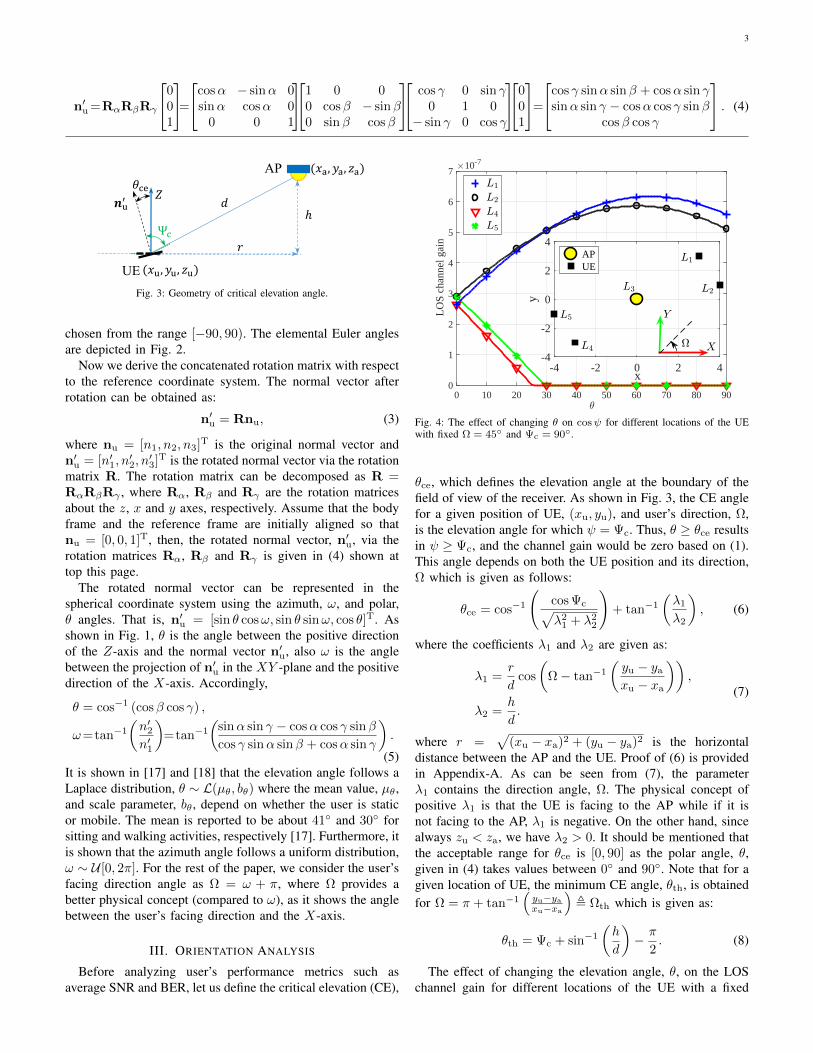
Fig. 3: Geometry of critical elevation angle.
chosen from the range [−90, 90). The elemental Euler anglesare depicted in Fig. 2.
Now we derive the concatenated rotation matrix with respectto the reference coordinate system. The normal vector afterrotation can be obtained as:
n′u = Rnu, (3)
where nu = [n1, n2, n3]T is the original normal vector andn′u = [n′1, n
′2, n′3]T is the rotated normal vector via the rotation
matrix R. The rotation matrix can be decomposed as R =RαRβRγ , where Rα, Rβ and Rγ are the rotation matricesabout the z, x and y axes, respectively. Assume that the bodyframe and the reference frame are initially aligned so thatnu = [0, 0, 1]T, then, the rotated normal vector, n′u, via therotation matrices Rα, Rβ and Rγ is given in (4) shown attop this page.
The rotated normal vector can be represented in thespherical coordinate system using the azimuth, ω, and polar,θ angles. That is, n′u = [sin θ cosω, sin θ sinω, cos θ]T. Asshown in Fig. 1, θ is the angle between the positive directionof the Z-axis and the normal vector n′u, also ω is the anglebetween the projection of n′u in the XY -plane and the positivedirection of the X-axis. Accordingly,
θ = cos−1 (cosβ cos γ) ,
ω=tan−1
(n′2n′1
)=tan−1
(sinα sin γ − cosα cos γ sinβ
cos γ sinα sinβ + cosα sin γ
).
(5)It is shown in [17] and [18] that the elevation angle follows aLaplace distribution, θ ∼ L(µθ, bθ) where the mean value, µθ,and scale parameter, bθ, depend on whether the user is staticor mobile. The mean is reported to be about 41 and 30 forsitting and walking activities, respectively [17]. Furthermore, itis shown that the azimuth angle follows a uniform distribution,ω ∼ U [0, 2π]. For the rest of the paper, we consider the user’sfacing direction angle as Ω = ω + π, where Ω provides abetter physical concept (compared to ω), as it shows the anglebetween the user’s facing direction and the X-axis.
III. ORIENTATION ANALYSIS
Before analyzing user’s performance metrics such asaverage SNR and BER, let us define the critical elevation (CE),
0 10 20 30 40 50 60 70 80 900
1
2
3
4
5
6
7
LO
S ch
anne
l gai
n
10-7
-4 -2 0 2 4x
-4
-2
0
2
4
y
APUE
Fig. 4: The effect of changing θ on cosψ for different locations of the UEwith fixed Ω = 45 and Ψc = 90.
θce, which defines the elevation angle at the boundary of thefield of view of the receiver. As shown in Fig. 3, the CE anglefor a given position of UE, (xu, yu), and user’s direction, Ω,is the elevation angle for which ψ = Ψc. Thus, θ ≥ θce resultsin ψ ≥ Ψc, and the channel gain would be zero based on (1).This angle depends on both the UE position and its direction,Ω which is given as follows:
θce = cos−1
(cos Ψc√λ2
1 + λ22
)+ tan−1
(λ1
λ2
), (6)
where the coefficients λ1 and λ2 are given as:
λ1 =r
dcos
(Ω− tan−1
(yu − ya
xu − xa
)),
λ2 =h
d.
(7)
where r =√
(xu − xa)2 + (yu − ya)2 is the horizontaldistance between the AP and the UE. Proof of (6) is providedin Appendix-A. As can be seen from (7), the parameterλ1 contains the direction angle, Ω. The physical concept ofpositive λ1 is that the UE is facing to the AP while if it isnot facing to the AP, λ1 is negative. On the other hand, sincealways zu < za, we have λ2 > 0. It should be mentioned thatthe acceptable range for θce is [0, 90] as the polar angle, θ,given in (4) takes values between 0 and 90. Note that for agiven location of UE, the minimum CE angle, θth, is obtainedfor Ω = π + tan−1
(yu−yaxu−xa
), Ωth which is given as:
θth = Ψc + sin−1
(h
d
)− π
2. (8)
The effect of changing the elevation angle, θ, on the LOSchannel gain for different locations of the UE with a fixed

4
TABLE I: Simulation Parameters
Parameter Symbol ValueAP location (xa, ya, za) (0, 0, 2)LED half-intensity angle Φ1/2 60
PD responsivity RPD 1 A/WPhysical area of a PD APD 1 cm2
Refractive index ς 1Downlink bandwidth B 10 MHzNumber of subcarriers K 1024Noise power spectral density N0 10−21 A2/HzConversion factor η 3Vertical distance of UE and AP h 2 m
0 45 90 135 180 225 270 315 360, [degree]
0
1
2
3
4
5
6
7
LO
S ch
anne
l gai
n
10-7
Fig. 5: The effect of changing Ω and θ on the LOS channel gain with Ψc =90, for different positions and elevation angles θ = 41 (solid lines), θ =θth (dash lines).
direction angle, Ω = 45 and Ψc = 90, is shown in Fig. 4.Here, Ψc =90 and other parameters are presented in Table I.It can be seen that for the UE’s locations of L4 = (−3,−3)and L5 =(−4,−1) by increasing the elevation angle, the LOSchannel gain decreases. After θce = 25.24 and θce = 29.5
for L4 and L5, respectively, the AP is out of the UE’s FOVand hence the LOS channel gains are zero. However, with thesame Ω=45 if the UE is located at positions like L1 =(3, 3)or L2 =(4, 1), the LOS channel gain does not become zero ifthe elevation angle changes between 0 and 90.
It is noted that under the condition of θ < θth the AP isalways within the UE’s field of view for any direction of Ω.For a given UE’s location, we are also interested in the rangeof Ω for which the LOS channel is active. Let’s denote thisrange as RΩ,θ. This range can be determined according to thefollowing Proposition.
Proposition. For a given UE’s location, the range of Ωfor which the LOS channel gain is non-zero is [0, 2π] if θis smaller than or equal to a threshold angle θth = Ψc +sin−1
(hd
)− π
2 . Otherwise it is given as follows:
RΩ,θ=
[0,Ωr1)
⋃(Ωr2, 2π], if Λ′(Ωr1) < 0
(Ωr1,Ωr2), if Λ′(Ωr1) ≥ 0, (9)
where Λ′(Ω) = −κ1 sin(
Ω− tan−1(yu−yaxu−xa
))+ κ2 with:
κ1 =r
dsin θ, κ2 =
h
dcos θ . (10)
0 0.5 1 1.5 2 2.5 30
0.2
0.4
0.6
0.8
1
4
Fig. 6: The effect of different FOV on having a zero LOS, PrH = 0.
Also Ωr1 = minΩ1,Ω2 and Ωr2 = maxΩ1,Ω2, where:
Ω1 = cos−1
(cos Ψc − κ2
κ1
)+tan−1
(yu − ya
xu − xa
),
Ω2 = − cos−1
(cos Ψc − κ2
κ1
)+tan−1
(yu − ya
xu − xa
).
(11)
Proof: See Appendix-B.The LOS channel gain versus Ω for locations of L1 and
L5 (see the inset of Fig. 4) with θ = θth (dash line) andθ = 41 ≥ θth (solid line) are shown in Fig. 5. Note thatfor L1 and L5, we have θth = 25.24 and θth = 25.88,respectively. As can be seen, if θ < θth, then, ∀Ω ∈ [0, 360),LOS channel gain is always non-zero (dash lines). Based onthe proposition, the range of Ω for which the LOS channel gainis non-zero with θ = 41 > θth is [0, 167.8)∪ (282.2, 360] forL1 and [70.1, 318] for L2.
It can be inferred form the Proposition that for a given UE’slocation and θ, the probability that the LOS path is not withinthe UE’s FOV (due to variation of Ω) is PrH = 0 = 1 −PrΩ ∈ RΩ,θ. Fig. 6 shows the PrH = 0 versus thehorizontal distance between the UE and the AP, r, for differentUE’s FOV. The results are shown for θ = 41. As can beobserved, PrH = 0 = 1, for UEs with a narrow FOV (i.e.,Ψc = 30 and 40) when they are located in the vicinity belowthe AP. As the horizontal distance, r, increases, PrH = 0first decreases and then it increases as it goes away from theAP. For wide FOVs (i.e., Ψc = 60, 80 and 90), PrH = 0is zero when the UE is in the vicinity below the AP, and thenit starts to increase at a certain r. This can be derived basedon (8) for Ψc ≥ θ that is r ≥ h tan(Ψc − θ). Note that thehigh value of losing the LOS link particularly for narrowerFOVs is due the fact that a single AP is considered and theeffect of reflection is ignored. A study of such effects has beenpresented in our recent work [23].
Let RΩ denote the range for which the LOS channel gain isalways non-zero regardless of θ, i.e., ∀θ ∈ [0, 90]. The range,RΩ, can be determined according to the following Corollary.
Corollary. For a given UE’s location, the range of Ω forwhich the LOS channel gain is non-zero for all θ ∈ [0, 90]

5
can be obtained as:
RΩ = RΩ,θ|For θ=90. (12)
Proof of this corollary is similar to the proof of proposition 1.Noting that the worst elevation angle that leads to the smallestrange of Ω is θ = 90. The physical concept of RΩ is thatwhen the UE faces the AP, we have Ω ∈ RΩ. Otherwise, if theUE faces the opposite direction of the AP, Ω /∈ RΩ. In fact,RΩ provides a stable range for which the user can change theelevation angle between 0 and 90 without experiencing theAP out of its FOV. We note that the range given in (12) isvalid if Ψc ≥ cos−1
(rd
)(this condition can be readily seen
by substituting θ = 90 in (10) and then replacing the resultsin (11)).
IV. BIT-ERROR RATIO PERFORMANCE
In this section, we evaluate the BER performance ofDCO-OFDM in LiFi networks. We initially derive the SNRstatistics on each subcarrier, then based on the derived PDFof SNR, the BER performance is assessed. Note that the PDFof the SNR derived in this study is the conditional PDF giventhe location and direction of the UE. Therefore, having thestatistics of the user location, the joint PDF of the SNR withrespect to both UE orientation and location can be readilyobtained.
A. SNR Statistics
The received electrical SNR1 on kth subcarrier of a LiFisystem can be acquired as:
S =R2
PDH2P 2
opt
(K − 2)η2σ2k
, (13)
where the PD responsivity is denoted by RPD; H is theLOS channel gain given in (1); Popt is the transmittedoptical power; K is the total number of subcarriers withK/2 − 1 subcarriers bearing information. Furthermore, η isthe conversion factor [26]. The condition η = 3 can guaranteethat less than 1% of the signal is clipped so that the clippingnoise is negligible [3], [27]. In (13), σ2
k = N0B/K is the noisepower on kth subcarrier where N0 stands for the noise spectraldensity and B represents the modulation bandwidth. Based onthe experimental measurement of the device orientation, it isshown in [17] that the LOS channel gain, H , follows a clippedLaplace distribution as:
fH(~)=exp
(− |~−µH|
bH
)bH
(2− exp
(−hmax−µH
bH
))+ cHδ(~), (14)
where δ(~) is the Dirac delta function, taking 1 if ~ = 0, and0 otherwise; cH = Fcosψ(cos Ψc), which is given as:
cH = Fcosψ(cos Ψc) ≈
1− 12 exp
(θce−µθbθ
), θce < µθ
12 exp
(− θce−µθbθ
), θce ≥ µθ
.
(15)
1Note that all SNR values throughout this paper are scalers, i.e., not in dB.
where bθ =√σ2θ/2. The parameters µθ and σθ are the
mean and standard deviation of the elevation angle, which areobtained based on the experimental measurements. For staticusers, they are reported as µθ = 41 and σθ = 7.68. Proof of(15) is provided in Appendix C. Furthermore, for the detailedproof of (14), we refer to Eq. (56) and (57) of [17]. The meanand scale factor of channel gain, µH and bH respectively, are:
µH =H0
dm+2(λ1 sinµθ + λ2 cosµθ) , (16)
bH =H0
dm+2bθ|λ1 cosµθ − λ2 sinµθ|, (17)
where H0 is given below (2). The factors, λ1 and λ2, are givenin (7). The support range of fH(~) is hmin ≤ ~ ≤ hmax wherehmin and hmax are given as:
hmin =
H0
dm+2 cos Ψc, cosψ < cos Ψc
H0
dm+2minλ1, λ2, o.w
, (18)
hmax =
H0
dm+2λ2, if λ1 < 0
H0
dm+2
√λ2
1 + λ22, if λ1 ≥ 0
. (19)
The cumulative distribution function (CDF) of LOS channelgain can be also obtained by calculating the integral of (14),which is given as:
FH(~) = cH+
exp(
~−µH
bH
)− exp
(hmin−µH
bH
)(2− exp
(−hmax−µH
bH
)) , hmin ≤ ~ ≤ µH
2− exp(hmin−µH
bH
)− exp
(−~−µH
bH
)(2− exp
(−hmax−µH
bH
)) , hmin ≤ µH ≤ ~
exp(−hmin−µH
bH
)− exp
(−~−µH
bH
)(2− exp
(−hmax−µH
bH
)) , µH ≤ hmin ≤ ~
.
(20)The relationship between channel gain and received SNR of
DCO-OFDM is given in (13). Using the fundamental theoremof determining the distribution of a random variable [28], thePDF of SNR can be obtained as follows:
fS(s) =fH(
√s/S0)
2S0
√s/S0
=exp
(− |√s−√S0µH|√S0bH
)2bH√S0s
(2− exp
(−hmax−µH
bH
)) + cHδ(s),
(21)
where S0 =R2
PDP2opt
(K−2)η2σ2k
and with the support range of s ∈(smin, smax), where smin = S0h
2min and smax = S0h
2max,
with hmin and hmax given in (18) and (19), respectively.By calculating the integral, FS(s) =
∫ ssmin
fS(s)ds, theCDF of SNR on k-th subcarrier can be obtained. The CDFof SNR can be also acquired by substituting ~ =
√sS0 in
(20), i.e., FS(s) = FH(√
sS0 ).
Fig. 7 shows the PDF and CDF of the receivedSNR obtained from analytical results compared with the

6
5 10 15 20 25 30 35 40 45SNR
0
0.4
0.8
1.2
1.6
2PD
F
Simulation PDFAnalytical model
0 10 20 30 40 50SNR
0
0.5
1
CD
FSimulation PDFAnalytical model
(a) Ω = 45
0 1 2 3 4 5 6SNR
0
0.2
0.4
0.6
0.8
1
PD
F
Simulation PDFAnalytical model
0 2 4 6 8SNR
0.97
0.98
0.99
1
CD
F
Simulation PDFAnalytical model
(b) Ω = 225
Fig. 7: Comparison between simulation and analytical results of PDF and CDF of received SNR for UE’s location L1 with Ω = 45 and Ω = 225.
Monte-Carlo simulation results. The UE is located at positionL1, the transmitted optical power is 3.2 W and UE’s FOV is90. The results are provided for two directions: Ω = 45 andΩ = 225. Other simulation parameters are given in Table I.As it can be seen, the analytical models for both PDF andCDF of the received SNR match the simulation results. Thefactor cH for Ω = 45 is 0. This factor for Ω = 225 is 0.975for simulation results and 0.979 for analytical model. Theseresults confirm the accuracy of the analytical model.
B. BER Performance
In this subsection, we aim to evaluate the effect of UEorientation on the BER performance of a LiFi-enabled deviceas one use case. BER is one of the common metrics to evaluatethe point-to-point communication performance. Assuming theM-QAM DCO-OFDM modulation, the average BER persubcarrier of the communication link can be obtained as [29]:
Pe =
∫ smax
smin
Pe (s) fS(s) ds, (22)
where Pe determines the BER of M -QAM DCO-OFDM inadditive white Gaussian noise (AWGN) channels, which canbe obtained approximately as [30]:
Pe(s) ≈ 4
log2M
(1− 1√
M
)Q
(√3s
M − 1
), (23)
where Q(·) is the Q-function. Substituting (21) and (23) into(22) and calculating the integral from smin to smax, we getthe average BER of the M -QAM DCO-OFDM in AWGNchannels with randomly-orientated UEs. After calculating theintegral and some simplifications, the approximated averageBER is given as:
Pe ≈
−∆0 + 1
2cHcM, µH ≤ hmin
Pe(S0µ2H) + 1
2cHcM, hmin < µH ≤ hmax
. (24)
0 0.5 1 1.5 2 2.5 3 3.5 4Transmitted optical power, P
opt , W
10-8
10-6
10-4
10-2
100
BE
R
Exact BERApprox. BERFixed Vertically upward UE
Fig. 8: BER performance of point-to-point communications for a UE locatedat L1. Three scenarios are considered: i) vertically upward UE, ii) UE withthe fixed polar angle without random orientation, and iii) real scenario witha random orientation (Laplace distribution) for polar angle.
where
∆0 =
2log2M
(1− 1√
M
)exp
(µH−hmin
bH
)(
2− exp(−hmax−µH
bH
)) ,
cM =4
log2M
(1− 1√
M
).
(25)
The proof is provided in Appendix D.Note that if the UE is tilted optimally towards the AP, the
BER is minimum. For any arbitrary location and direction ofUE, the optimum tilt (OT) angle is defined as the angle thatprovides maximum channel gain [8], [9], [31], [32]. This angleis θot = tan−1
(λ1
λ2
)and the average BER for this tilt angle is
Pe ≈ Pe(S0µ2H) (since cH = 0).
Fig. 8 illustrates the BER performance of 4-QAMDCO-OFDM for three scenarios: i) a vertically upward UE, ii)

7
a UE with a fixed polar angle and without random orientationiii) a realistic scenario in which the polar angle follows aLaplace distribution that considers the random orientation, i.e.,θ ∼ L(µθ, bθ). Here, we assume µθ = 41 and bθ = 5.43
as reported in [17] based on the experimental measurements.Other simulation parameters are given in Table I. The resultsare provided for the UE’s location of L1 = (3, 3) and withΨc = 60. For this location, θot ≈ 65. Some interestingobservations can be seen from the results shown in this figure.As can be seen, for Ω = 45, the vertically upward UE fallsbehind the other two scenarios. Because for θ > 0, the UEwill be tilted towards the AP (see the results shown in Fig. 4).Also, the gap between the exact and approximate BER issmall which confirms the accuracy of the BER approximation.One interesting observation is that after Popt > 2 W andPopt > 2.5 W, the BER does not decrease and is saturatedfor θ = 41 and θ = θot, respectively. This is due to theconstant term in (24), i.e., 1
2cHcM, will be dominant comparedto the power-dependent term, i.e., Pe(S0µ
2H). In other words,
due to the random orientation, there are cases that LOS link isout of the UE’s FOV and data is lost. These results highlightthe significance of considering the random orientation in theperformance assessment. The BER performance of second andthird scenarios can still be better if θ = θot ≈ 65. For θ = θot
the maximum LOS channel gain is achieved and under thiscondition the BER is minimum. This fact underlines that thedevice orientation is not always destructive. Furthermore, withθ = θot the UE’s random orientation has the minimum effecton the BER. We note that for a given location and Ω, the Pe
given in (24) is always bounded to the BER of Pe(s) obtainedfor θ = θot as it provides the maximum LOS channel gain.The BER results of θ = θot are just provided for a comparisonpurpose however, the users tends to keep their smartphonewith θ = 41 (when doing sitting activities) according to theexperimental measurements [17].
C. UE’s Random Motion
In this subsection, we will include the effect of UE’s randommotion even though the user is static in addition to the randomorientation on the BER performance. Note that here, therandom UE’s motion encompass small movements in x, yand z directions, which are modeled as Gaussian distributions.Hence, the UE’s location at each realization is given as:
(xu, yu, zu) = (x0,u, y0,u, z0,u) + (∆x,∆y,∆z), (26)
where ∆x ∼ N (x0,u, σ2x), ∆y ∼ N (y0,u, σ
2y) and ∆z ∼
N (z0,u, σ2z ). The location (x0,u, y0,u, z0,u) denotes the mean
point that the UE fluctuates around. It is noted that typicallythe variation of the UE’s height (along z axis) is less than thevariation along x and y axes.
Fig. 9 shows the effect of random motion along with randomorientation on the BER performance. In these simulations, weassume that σx = σy = 5σz = σ. The results are presentedfor three values of σ, which are 0.05 m, 0.1 m and 0.15 m.Note that for σ = 0.15 m, the deviation of the UE’s locationfrom the mean point, (x0,u, y0,u, z0,u), can be in the range of−3σ = −45 cm to 3σ = 45 cm. This corresponds to high
0 0.5 1 1.5 2 2.5 3 3.5 410-8
10-6
10-4
10-2
100
BE
R
, W
Fig. 9: The effect of random orientation with/without random motion on BERperformance of a UE located at the arbitrary position of L1.
AP1
AP2
𝑟h
UE
Fig. 10: Geometry of two APs with interference consideration. APs are locatedat (−2, 0) and (2, 0) on the ceiling.
UE’s motion which is very low probable for normal humanactivities. Here, the modulation order is considered to be M =4. The simulations are carried out for a UE located at L1 =(3, 3) with different Ω and µθ. The UE’s FOV is assumed tobe 90 for these simulations. As it can be seen, with σ ∈0.05, 0.1, the gap between the results when random motionis included, is indeed negligible. For the case of Ω = 135
and µθ = 41 and with σ = 0.15 m, the gap is still small. ForΩ = 45 and µθ = 41 (or µθ = 65) with σ = 0.15 m, thegap grows in high transmitted power.
D. Multiple APs Scenario
To investigate the effect of multiple APs on the errorperformance of a randomly-orientated UE, we consider twoAPs located at (−2, 0) and (2, 0) as shown in Fig. 10. Thesignal-to-interference- plus-noise ratio (SINR) can be obtainedas:
Υ =R2
PDH2dP
2opt
(K − 2)η2(σ2k + I)
, (27)
where Hd is the LOS channel gain between the desired AP andthe PD; I is the interfering power from other APs on the kthsubcarrier. Other parameters are defined below (13). Here, withthe consideration of two APs, the interference from the otherAP on the kth subcarrier is I = R2
PDH2inP
2opt/((K − 2)η2),
where Hin is the channel gain between the interfering APand the UE. Note that the desired AP is selected basedon the received signal intensity metric. Fig. 11 shows the

8
0 1 2 3 4 5 60
20
40
60
80
100
120A
vera
ge S
INR
60 70 80 90SINR
0
0.05
0.1
0.15
5 10 15 20 25SINR
0
0.1
0.2
Fig. 11: Average SINR versus the horizontal distance of the UE and first AP,rh, (see the geometry shown in Fig. 10).
average SINR versus different horizontal distances betweenthe UE and first AP (as depicted in Fig. 10). The average istaken over different random orientations following a Laplacedistribution based on the experimental measurements, i.e.,θ ∼ L(41, 5.43). Note that mobility is not considered inthese results and at each location the user is assumed to besitting. The simulation parameters are given in Table I andthe UE’s FOV is assumed to be 90. The transmitted opticalpower per AP is supposed to be 1 W as multiple APs requirelower transmit power to cover the room in comparison to thesingle AP case. The PDF of SINR for rh = 1 with Ω = 0and rh = 4.5 with Ω = 90 are presented. For the formerthe average SINR is about 82 while for the latter, it is about16. Note also that the PDF of SINR shows similar Laplaciandistributions as in the SNR case.
V. CONCLUSIONS AND FUTURE WORKS
We analyzed the device orientation and assessed itsimportance on system performance. The PDF of SNR forrandomly-orientated device is derived, and based on thederived PDF, the BER performance of DCO-OFDM inAWGN channel with randomly-orientated UEs is evaluated.An approximation for the average BER of randomly-orientedUEs is calculated that closely matches the exact one. The roleof CE angle that guarantees having LOS link in the UE’sFOV is investigated. Furthermore, the significant impact ofbeing optimally tilted towards the AP on the BER performanceis shown. We also studied the effect of the UE’s randommotion on the BER performance. We note that even thoughwe considered DCO-OFDM, the methodology can be readilyextended to other modulation schemes, which can be the focusof future studies. Furthermore, other performance metricssuch as throughput and user’s quality of service can also beassessed. Also, the device orientation impact can be evaluatedin a cellular network with consideration of non-line-of-sightlinks.
ACKNOWLEDGMENT
M.D. Soltani acknowledges the School of Engineering forproviding financial support. Harald Haas and Majid Safarigratefully acknowledge financial support from EPSRC undergrant EP/L020009/1 (TOUCAN).
APPENDIX
A. Proof of (6)Recalling that cosψ = −d · n′u/d, replacing for d = [xu −
xa, yu−ya, zu−za]T and n′u = [sin θ cosω, sin θ sinω, cos θ]T
and also noting that ω = Ω + π, we have:
cosψ =(xu − xa)sin θ cos Ω + (yu − ya)sin θ sin Ω− (zu − za)cos θ√
(xu − xa)2 + (yu − ya)2 + (zu − za)2
=
√(xu − xa)2+ (yu − ya)2 sin θ cos
(Ω− tan−1
(yu − ya
xu − xa
))− (zu− za)cos θ√
(xu − xa)2 + (yu − ya)2 + (zu − za)2
=r
dsin θ cos
(Ω− tan−1
(yu − ya
xu − xa
))+h
dcos θ.
(28)For a given location of UE and a fixed angle of Ω, by usingthe simple triangular rules, cosψ can be represented as:
cosψ =λ1 sin θ + λ2 cos θ =√λ2
1 + λ22 cos
(θ − tan−1
(λ1
λ2
)),
(29)where λ1 and λ2 are given as:
λ1 =r
dcos
(Ω− tan−1
(yu − ya
xu − xa
)),
λ2 =h
d.
(30)
According to the definition of critical elevation angle, if θ =θce, then, cosψ = cos Ψc. Therefore, (29) results in:
θce = cos−1
(cos Ψc√λ2
1 + λ22
)+ tan−1
(λ1
λ2
). (31)
This completes the proof of the derivation of CE angle.
B. Proof of Proposition
For a given location of UE and a fixed elevation angle,one other representation of cosψ given in (28) would be as afunction of Ω:
cosψ=κ1 cos
(Ω− tan−1
(yu − ya
xu − xa
))+ κ2 , Λ(Ω), (32)
where the coefficients κ1 and κ2 are given as:
κ1 =r
dsin θ, κ2 =
h
dcos θ. (33)
Note that since θ ∈ [0, 90], we have κ1 ≥ 0 and κ2 ≥ 0. Asmentioned for θ = θce, we have cosψ = cos Ψc. Then, solvingΛ(Ω) − cos Ψc = 0 for Ω, the roots are Ωr1 = minΩ1,Ω2and Ωr2 = maxΩ1,Ω2, where Ω1 and Ω2 are given asfollow:
Ω1 = cos−1
(cos Ψc − κ2
κ1
)+tan−1
(yu − ya
xu − xa
),
Ω2 = − cos−1
(cos Ψc − κ2
κ1
)+tan−1
(yu − ya
xu − xa
).
(34)

9
For the special case of Ψc = 90, (34) is simplified as:
Ω1 =cos−1
(−h cot θ
r
)+ tan−1
(yu − ya
xu − xa
),
Ω2 =− cos−1
(−h cot θ
r
)+ tan−1
(yu − ya
xu − xa
).
(35)
Using the sinuous function properties if Λ(Ω) ≤ 0 forΩ ∈ [Ωr1,Ωr2], then the derivative of Λ(Ω) at Ω = Ωr1 isnegative, i.e., ∂Λ(Ω)
∂Ω |Ω=Ωr1 < 0. For simplicity of notation,let’s denote Λ′(Ω) = ∂Λ(Ω)
∂Ω . Using (32), we have Λ′(Ω) =
−κ1 sin(
Ω− tan−1(yu−yaxu−xa
))+ κ2. Therefore, the range of
RΩ that guarantees Λ(Ω) > 0 would be [0,Ωr1)⋃
(Ωr2, 2π].Similarly, if Λ(Ω) ≥ 0 for Ω ∈ (Ωr1,Ωr2), then the derivativeof Λ(Ω) at Ω = Ωr1 is positive, i.e., ∂Λ(Ω)
∂Ω |Ω=Ωr1> 0.
Consequently, in this case the range of RΩ that ensuresΛ(Ω) > 0 would be [Ωr1,Ωr2]. This completes the proof ofProposition.
C. Proof of (15)Using (29), the CDF of cosψ can be obtained as:
Fcosψ(τ) = Prcosψ ≤ τ
= Pr
√λ2
1 + λ22 cos
(θ − tan−1
(λ1
λ2
))≤ τ
= 1− Fθ
(cos−1
(τ√
λ21 + λ2
2
)+ tan−1
(λ1
λ2
)).
(36)
where Fθ(θ) is the CDF of the elevation angle, θ. Under theassumption of Laplacian model for the elevation angle, Fθ(θ)is given as [17]:
Fθ(θ) =
1
2(G(π2 )−G(0))exp
(θ−µθbθ
), θ < µθ
1− 1
2(G(π2 )−G(0))exp(− θ−µθbθ
), θ ≥ µθ
. (37)
where G(0)= 12 exp
(−µθbθ
)and G(π2 ) = 1− 1
2 exp(−
π2−µθbθ
).
Note that with reported values for µθ and bθ from [17], wehave
(G(π2 )−G(0)
)≈ 1. Therefore,
Fθ(θ) ≈
12 exp
(θ−µθbθ
), θ < µθ
1− 12 exp
(− θ−µθbθ
), θ ≥ µθ
. (38)
Finally, by recalling the definition of the CE angle given in(6), Fcosψ(cos Ψc) can be approximately obtained as:
Fcosψ(cos Ψc)≈
1− 12 exp
(θce−µθbθ
), θce < µθ
12 exp
(− θce−µθbθ
), θce ≥ µθ
. (39)
This completes the proof of (15).
D. Proof of (24)Substituting (21) and (23) into (22), we have:
Pe = c0
∫ smax
smin
Q
(√3s
M − 1
)1√s
exp
(−|√s−√S0µH|√
S0bH
)ds
+ cHcM
∫ smax
smin
Q
(√3s
M − 1
)δ(s)ds
(40)
with c0 and cM given as:
c0 =cM
2bH√S0
(2− exp
(−hmax−µH
bH
)) ,cM =
4
log2M
(1− 1√
M
).
(41)
Note that if smin = 0, the second integral in (40) iscHcMQ(0) = cHcM
2 , and referring to the definition of cH, it iszero for smin > 0. Thus, the second integral can be expressedas cHcM
2 and we need to simplify the first integral. For
simplicity of notation, let define c1 =√
3M−1 , c2 =
√S0µH
and c3 =√S0bH. Furthermore, let x =
√s, thus, the first
integral in (40) can be rewritten as (42) given at the topof the next page. The right side of (42) is based on thebehavior of PDF of SNR. It can be either single exponential (ifc2 ≥
√smin) or double exponential (if
√smin < c2 ≤
√smax),
for example, see results shown in Fig. 7. Noting that∫Q(c1x)e
xc3 dx =
c3exc3Q(c1x) +
c32e
1
4c21c23
(1− 2Q
(c1x−
1
2c1c3
)),
(43)
also for given values of c1, c2 and c3, we have Q(c1c2) ≈Q(c1
√smax) and also since µH >> bH, then, e−
c2c3 ≈ 0.
Hence, Pe can be approximated by (44) presented at the topof the next page. By substituting for the values of c0, c1, c2, c3and noting that
√smin =
√S0hmin and
√smax =
√S0hmax
(44) can be rewritten as:
Pe≈
−
2log2M
(1− 1√
M
)eµH−hmin
bH(2−exp
(−hmax−µH
bH
)) + cHcM2 , µH ≤ hmin
4(
1− 1√M
)log2M
Q
(√3S0µ2
H
M−1
)+ cHcM
2 , hmin < µH ≤ hmax
.
(45)This completes the proof of (24).
REFERENCES
[1] Cisco, “Cisco Visual Networking Index: Global Mobile Data TrafficForecast Update, 2016–2021 White Paper,” white paper at Cisco.com,Mar. 2017.
[2] H. Haas, L. Yin, Y. Wang, and C. Chen, “What is LiFi?” Journal ofLightwave Technology, vol. 34, no. 6, pp. 1533–1544, Mar. 2016.
[3] M. D. Soltani, X. Wu, M. Safari, and H. Haas, “Bidirectional UserThroughput Maximization Based on Feedback Reduction in LiFiNetworks,” IEEE Transactions on Communications, vol. 66, no. 7, pp.3172–3186, 2018.
[4] I. Tavakkolnia, C. Chen, R. Bian, and H. Haas, “Energy-EfficientAdaptive MIMO-VLC Technique for Indoor LiFi Applications,” inICT 2018, 25th International Conference on Telecommunications.Saint-Malo, France: IEEE, June 2018.
[5] M. D. Soltani, X. Wu, M. Safari, and H. Haas, “Access Point Selection inLi-Fi Cellular Networks with Arbitrary Receiver Orientation,” in 2016IEEE 27th Annual International Symposium on Personal, Indoor, andMobile Radio Communications (PIMRC), Valencia, Spain, Sept 2016,pp. 1–6.
[6] M. D. Soltani, H. Kazemi, M. Safari, and H. Haas, “Handover Modelingfor Indoor Li-Fi Cellular Networks: The Effects of Receiver Mobilityand Rotation,” in 2017 IEEE Wireless Communications and NetworkingConference (WCNC), San Fransisco, USA, March 2017, pp. 1–6.
[7] A. A. Purwita, M. D. Soltani, M. Safari, and H. Haas, “HandoverProbability of Hybrid LiFi/RF-based Networks with Randomly-OrientedDevices,” in 2018 87th Vehicular Technology Conference(VTC2018-Spring), Porto, Portugal, June 2018.

10
∫ √smax
√smin
Q(c1x)e−|x−c2|c3 dx =
∫√smax√
sminQ(c1x)e−
x−c2c3 dx, c2 ≤
√smin∫ c2√
sminQ(c1x)e
x−c2c3 dx+
∫√smax
c2Q(c1x)e−
x−c2c3 dx,
√smin < c2 ≤
√smax
,(42)
Pe ≈
−c0c3 + cHcM2 , c2 ≤
√smin
2c0c3Q(c1c2)
(2− e
c2−√smaxc3
)+ cHcM
2 ,√smin < c2 ≤
√smax
. (44)
[8] J. Y. Wang, Q. L. Li, J. X. Zhu, and Y. Wang, “Impact of Receiver’sTilted Angle on Channel Capacity in VLCs,” Electronics Letters, vol. 53,no. 6, pp. 421–423, Mar. 2017.
[9] J. Y. Wang, J. B. Wang, B. Zhu, M. Lin, Y. Wu, Y. Wang, and M. Chen,“Improvement of BER Performance by Tilting Receiver Plane for IndoorVisible Light Communications with Input-Dependent Noise,” in 2017IEEE International Conference on Communications (ICC), Paris, France,May 2017, pp. 1–6.
[10] Z. Wang, C. Yu, W.-D. Zhong, and J. Chen, “PerformanceImprovement by Tilting Receiver Plane in M-QAM OFDM Visible LightCommunications,” Optics Express, vol. 19, no. 14, pp. 13 418–13 427,2011.
[11] C. Le Bas, S. Sahuguede, A. Julien-Vergonjanne, A. Behlouli,P. Combeau, and L. Aveneau, “Impact of Receiver Orientation andPosition on Visible Light Communication Link Performance,” in OpticalWireless Communications (IWOW), 2015 4th International Workshop on.Istanbul, Turkey: IEEE, 2015, pp. 1–5.
[12] A. A. Matrawy, M. El-Shimy, M. Rizk, Z. El-Sahn et al., “OptimumAngle Diversity Receivers for Indoor Single User MIMO VisibleLight Communication Systems,” in Asia Communications and PhotonicsConference. Wuhan, China: Optical Society of America, 2016, pp.AS2C–4.
[13] Y. S. Eroglu, Y. Yapici, and I. Guvenc, “Impact of Random ReceiverOrientation on Visible Light Communications Channel,” arXiv preprintarXiv:1710.09764, 2017.
[14] Vieyra Software. Physics toolbox sensor suite.[Online]. Available: https://play.google.com/store/apps/details?id=com.chrystianvieyra.physicstoolboxsuite
[15] M. D. Soltani, M. Safari, and H. Haas, “On Throughput MaximizationBased on Optimal Update Interval in Li-Fi Networks,” in Personal,Indoor, and Mobile Radio Communications (PIMRC), 2017 IEEE 28thAnnual International Symposium on. Montreal, QC, Canada: IEEE,Oct 2017, pp. 1–6.
[16] M. D. Soltani, X. Wu, M. Safari, and H. Haas, “On Limited FeedbackResource Allocation for Visible Light Communication Networks,”in Proceedings of the 2nd International Workshop on Visible LightCommunications Systems. Paris, France: ACM, Sept 2015, pp. 27–32.
[17] M. D. Soltani, A. A. Purwita, Z. Zeng, H. Haas, and M. Safari,“Modeling the Random Orientation of Mobile Devices: Measurement,Analysis and LiFi Use Case,” IEEE Transactions on Communications,pp. 1–1, 2018.
[18] A. A. Purwita, M. D. Soltani, M. Safari, and H. Haas, “Impactof Terminal Orientation on Performance in LiFi Systems,” in 2018IEEE Wireless Communications and Networking Conference (WCNC),Barcelona, Spain, April 2018.
[19] Z. Zeng, M. D. Soltani, H. Haas, and M. Safari, “Orientation Model ofMobile Device for Indoor VLC and Millimetre Wave Systems,” in 2018IEEE 88nd Vehicular Technology Conference (VTC2018-Fall), Chicago,USA, August 2018.
[20] M. D. Soltani, M. A. Arfaoui, I. Tavakkolnia, A. Ghrayeb, M. Safari,C. Assi, M. Hasna, and H. Haas, “Bidirectional Optical SpatialModulation for Mobile Users: Towards a Practical Design for LiFiSystems,” arXiv preprint arXiv:1812.03109, 2018.
[21] I. Tavakkolnia, M. D. Soltani, M. A. Arfaoui, , A. Ghrayeb, C. Assi,M. Safari, and H. Haas, “MIMO System with Multi-directional Receiverin Optical Wireless Communications,” in 2019 IEEE Int. Conf. onCommunications Workshops (ICC Workshops), Shanghai, China, May2019, pp. 1–6.
[22] C. Chen, M. D. Soltani, M. Safari, A. A. Purwita, X. Wu, andH. Haas, “An Omnidirectional User Equipment Configuration to SupportMobility in LiFi Networks,” in 2019 IEEE International Conference on
Communications Workshops (ICC Workshops), Shanghai, China, May2019, pp. 1–6.
[23] A. A. Purwita, M. D. Soltani, M. Safari, and H. Haas, “TerminalOrientation in OFDM-based LiFi Systems,” arXiv preprintarXiv:1808.09269, 2018.
[24] J. M. Kahn and J. R. Barry, “Wireless Infrared Communications,” Proc.IEEE, vol. 85, no. 2, pp. 265–298, Feb. 1997.
[25] C. Barthold, K. P. Subbu, and R. Dantu, “Evaluation ofGyroscope-Embedded Mobile Phones,” in Proc. IEEE Int. Conf.Syst. Man Cybernetics (SMC), Oct. 2011, pp. 1632–1638.
[26] S. D. Dissanayake and J. Armstrong, “Comparison of ACO-OFDM,DCO-OFDM and ADO-OFDM in IM/DD Systems,” Journal ofLightwave Technology, vol. 31, no. 7, pp. 1063–1072, 2013.
[27] S. Dimitrov and H. Haas, “Optimum Signal Shaping in OFDM-BasedOptical Wireless Communication Systems,” in 2012 IEEE VehicularTechnology Conference (VTC Fall), Quebec City, QC, Canada, Sept2012, pp. 1–5.
[28] A. Papoulis and S. U. Pillai, Probability, Random Variables, andStochastic Processes and Queueing Theory. Tata McGraw-HillEducation, 2002.
[29] Z. Ghassemlooy, W. Popoola, and S. Rajbhandari, Optical WirelessCommunications: System and Channel Modelling with Matlab. CRCpress, 2012.
[30] S. Dimitrov, S. Sinanovic, and H. Haas, “Clipping Noise inOFDM-Based Optical Wireless Communication Systems,” IEEETransactions on Communications, vol. 60, no. 4, pp. 1072–1081, April2012.
[31] E.-M. Jeong, S.-H. Yang, H.-S. Kim, and S.-K. Han, “Tilted ReceiverAngle Error Compensated Indoor Positioning System Based on VisibleLight Communication,” Electronics Letters, vol. 49, no. 14, pp. 890–892,2013.
[32] M. D. Soltani, Z. Zeng, I. Tavakkolnia, H. Haas, and M. Safari, “RandomReceiver Orientation Effect on Channel Gain in LiFi Systems,” in 2019IEEE Wireless Communications and Networking Conference (WCNC),Marrakech, Morocco, April 2019, pp. 1–6.