IMPACT EVALUATION: IMPACT EVALUATION: INSTRUMENTAL VARIABLE INSTRUMENTAL VARIABLE

METHOD METHOD SHAHID KHANDKER

World BankJune 2006

ORGANIZED BY THE WORLD BANK AFRICA IMPACT EVALUATION INITIATIVEIN COLLABORATION WITH HUMAN DEVELOPMENT NETWORK

AND WORLD BANK INSTITUTE

REPUBLIC OF SOUTH AFRICAGOVERNMENT-WIDE MONITORING & IMPACT EVALUATION SEMINAR

2

The main objective of Impact Evaluation…….

• To estimate the treatment effect of an intervention T on an outcome Y

• For example:– What is the effect of an increase in the minimum

wage on employment?– What is the effect of a school feeding program on

learning outcomes?– What is the effect of a training program on

employment and earnings?– What is the effect of micro-finance participation on

consumption and employment?

3

What would have happened to the beneficiaries if the program

had not existed?

What would have happened to the beneficiaries if the program

had not existed?

The Counterfactual

Recall the evaluator’s key question is:

How do you rewrite history? How do youget baseline data?

4

In theory, a single observation is not enough

Effect or impact = 13

With equivalent control group.

Extreme care must be taken when selecting the control group to ensure comparability.

Inco

me

leve

l

TimeProgram

30

10

17

The Ideal strategy

BeneficiariesEquivalent control group

5

Problem with ideal strategy is:

• Ethical problem (to condemn a group to not being beneficiaries)

• Difficulties associated with finding an equivalent group outside the project

• Costs• People change behaviour over time

It is extremely difficult to assemble an exactly comparable control group:

Therefore, this approach is practically difficult

6

Examples of less than ideal strategies…• Comparing individuals before and after the

intervention• Comparing individuals that participated in the

intervention to those that did not

• Example of a micro-credit program – Often targeted – not everyone is eligible– Some individuals chose to participate and some don’t even

among the eligible households/individuals

– Why can’t we estimate the program’s impact by comparing outcomes of participants to non-participants?

7

Findings on the impact are

inconclusive

Effect or impact?

Inco

me

leve

l

Time

Program

30

10

1714

21Base Line

Study

Time series

?

Broad descriptive surveyBeneficiaries

Example with less than ideal strategies such as using a before/after comparison

8

Effect or impact = 13

Projection for beneficiaries if no policy

Time

Program

30

10

17

Inco

me

leve

l

14

21

Comparison with non-equivalent control group

Beneficiariescontrol group

Data on before and after

situations is needed.

9

Micro-credit program• Participation is a choice variable

endogenous• Observed and unobserved characteristics

about participants that make them different from those who did not participate– Omitted variables – can control for many

observed characteristics, but are still missing things that are hard or impossible to measure

– Our treatment effect is “picking up” the effect of other characteristics that explain treatment, resulting in a biased estimate of the treatment effect

10

Micro-credit program

• Estimation: compare outcomes of individuals that chose to participate to those who did not:

Where T = 1 if enrolled in programT = 0 if not enrolled in programx = exogenous regressors (i.e. controls)

• The problem:– Corr (T , ε) ≠ 0

1 2y T xα β β ε= + + +

11

Micro-credit Program• Examples of why Corr (T , ε) ≠ 0

• Different motivation• Different ability• Different information• Different opportunity cost of participating• Different level of access

• There are characteristics of the treated that should be in ε, but are being “picked up” byT.

• We have violated one of the key assumptions of OLS: Independence of regressors x from disturbance term ε

12

What can we do about this problem?

• Try to “clean up” the correlation between T and ε:

• Isolate the variation in T that is uncorrelated with ε

• To do this, we need to find an instrumental variable (IV)

• OR, design programs with instrumental variables in mind

13

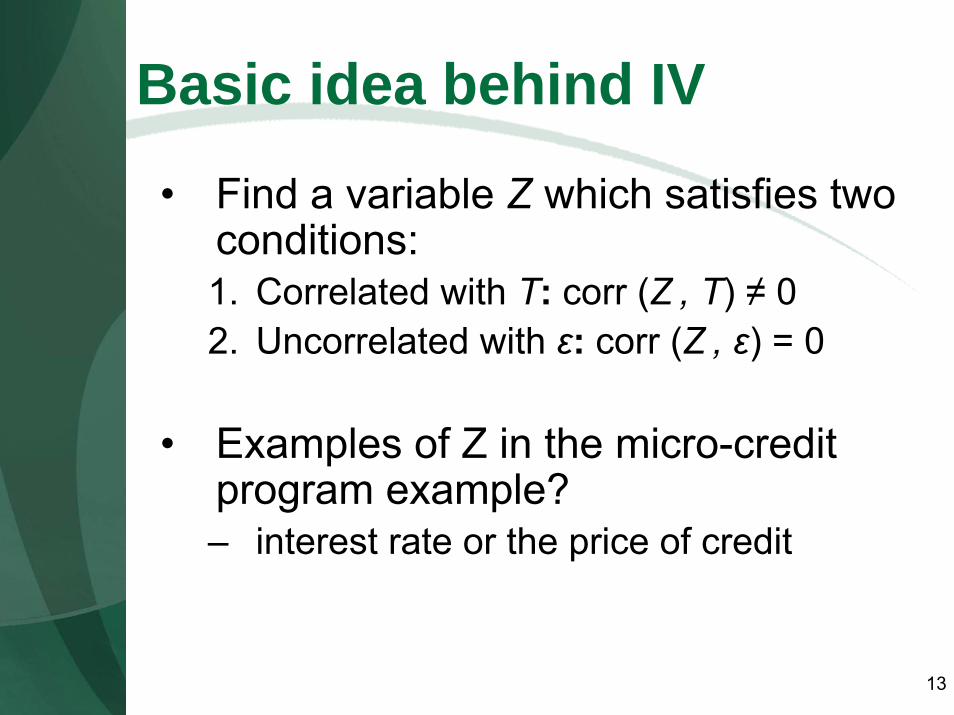
Basic idea behind IV

• Find a variable Z which satisfies two conditions:1. Correlated with T: corr (Z , T) ≠ 02. Uncorrelated with ε: corr (Z , ε) = 0

• Examples of Z in the micro-credit program example? – interest rate or the price of credit

14

Two Stage Least Squares (2SLS)

• Stage 1: Regress endogenous variable on the IV (Z) and other exogenous regressors

– Calculate predicted value for each observation: T hat

1 2y T xα β β ε= + + +

0 1 1T x Zδ δ θ τ= + + +

15

Two stage Least Squares (2SLS)• Stage 2: Regress outcome y on

predicted variable (and other exogenous variables)

– Need to correct Standard Errors (they are based on T hat rather than T)

• In practice just use STATA - ivreg• Intuition: T has been “cleaned” of its

correlation with ε.

^

1 2( )y T xα β β ε= + + +

16

Two stage Least Squares (2SLS)• Another way of presenting the same resul

• β1= Cov(y,z|X)/Cov(T,z)

• Cov(y,z) is called “The Reduced Form”

• Cov(T,z) is called “The First Stage”

17

Example: Grameen Bank impact

• C is credit demand;• Y is outcome variable (consumption,

assets, employment, schooling, family planning);

• Subscripts: household i; village j; male m; female f; time t;

• Want to allow separate effects on outcome of male and female credit;

• X represents individual or household characteristics.

18

Measuring Impacts: Cross-Sectional data

Credit demand equations: Cijm = Xijmβc + Zijmγc + μcjm + εc

ijmCijf = Xijfβc + Zijfγc + μcjf + εc

ijf

Outcome equation: Yij = Xij βy + Cijm δm + Cijf δf + μyj + εy

ij

Note: the Z represent variables assumed toaffect credit demand but to have no directeffect on the outcome.

19

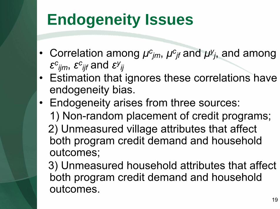
Endogeneity Issues

• Correlation among μcjm, μcjf and μyj, and among εcijm, εcijf and εyij

• Estimation that ignores these correlations have endogeneity bias.

• Endogeneity arises from three sources:1) Non-random placement of credit programs; 2) Unmeasured village attributes that affect both program credit demand and household outcomes;3) Unmeasured household attributes that affect both program credit demand and household outcomes.

20

Resolving endogeneity

• Village-level endogeneity – resolved by village FE;

• Household-level endogeneity – resolved by instrumental variables (IV);

• In credit demand equation Zijm and Zijfrepresent instrumental variables;

• Selecting Zij variables is difficult;Possible solution: identification using quasi-experimental survey design.

21

Quasi-experimental survey design

• Households are sampled from program and non-program villages;

• Both eligible and non-eligible households are sampled from both types of villages;

• Both participants and non-participants are sampled from eligible households.

Identification conditions:• Exogenous land-holding;• Gender-based program design.

22

Instruments for identification• Exogenous land-holding criteria:

- Only households owning up to 0.5 acre of land qualify for program participation. In practice there is some deviation from this cutoff.

• Gender-based program participation criteria:- Male members of qualifying households

cannot participate in program if village does not have a male program group. - Female members of qualifying households

cannot participate in program if village does not have a female program group.

23

Construction of Zij variables

Male choice=1 if household has up to 0.5 acreof land and village has male credit group

=0 otherwiseFemale choice=1 if household has up to 0.5acre of land and village has female credit group

=0 otherwiseMale and female choice variables are interacted

with household characteristics to form ZijVariables.

24

What this means…..

Intuitively, the outcome regression now relates variation in Y to variation in Cassociated with variation in Z.

25

Table 1: Weighted Mean and Standard Deviations of Dependent VariablesDependent Variables

Partici-pants

Obs. Non-partici-pants

Obs. Total Obs. Non-program areas

Obs. Aggregate Obs.

Sum of program loans of females (Taka)

5498.854(7229.351)

779 326 2604.454(5682.398)

1105- - 2604.454(5682.398)

1105

Sum of program loans by males (Taka)

3691.993(7081.581)

631 - 263 1729.631(5184.668)

894 - - 1729.631(5184.668)

895

Per capita HH weekly food expenditure (Taka)

59.166(19.865)

2696 62.265(23.256)

1650 61.242(22.239)

4326 61.985(23.897)

872 61.366(22.522)

5218

Per capita HH weekly non-food expenditure (Taka)

17.848(31.538)

2696 23.621(54.791)

1650 21.716(48.439)

4346 27.676(51.409)

872 22.706(48.990)

5218

Per capita HH total weekly expenditure (Taka)

77.014(41.496)

2696 85.886(64.820)

1650 82.959(58.309)

4346 89.661(66.823)

872 84.072(59.851)

5218

26

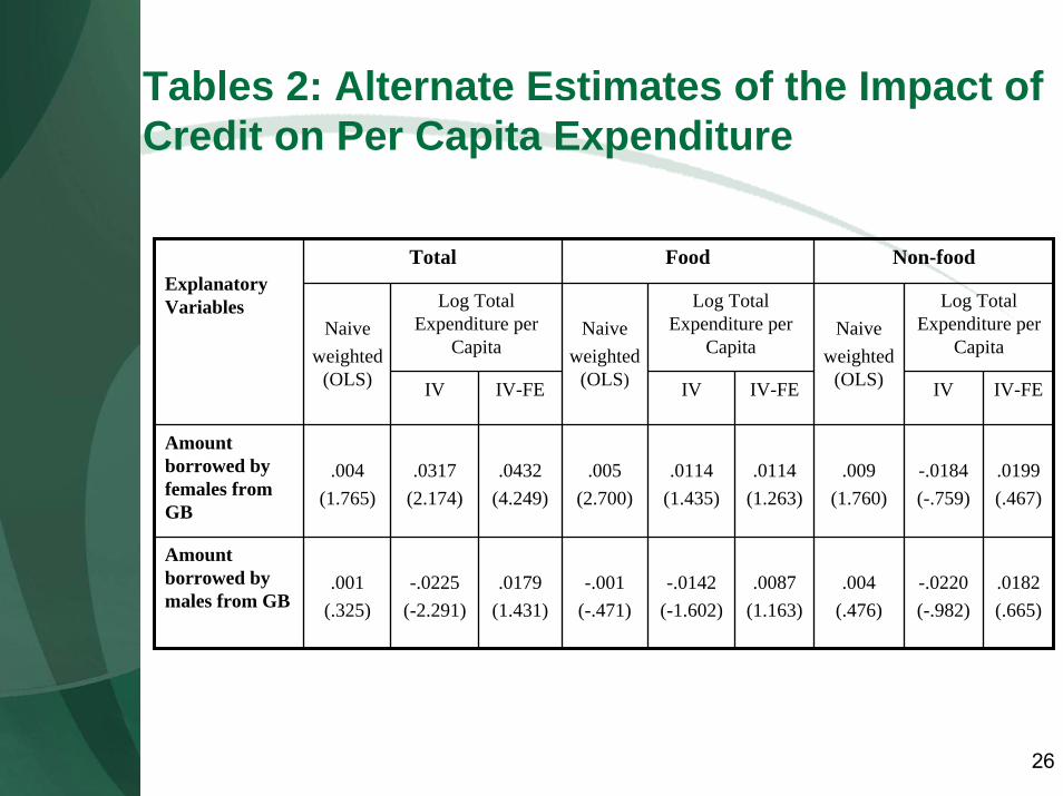
Tables 2: Alternate Estimates of the Impact of Credit on Per Capita Expenditure

Total Food Non-food

Log Total Expenditure per

Capita

Log Total Expenditure per

Capita

Log Total Expenditure per

Capita

IV IV-FE IV IV-FE IV IV-FE

Amount borrowed by females from GB

.004(1.765)

.0317(2.174)

.0432(4.249)

.005(2.700)

.0114(1.435)

.0114(1.263)

.009(1.760)

-.0184(-.759)

.0199(.467)

Amount borrowed by males from GB

.001(.325)

-.0225(-2.291)

.0179(1.431)

-.001(-.471)

-.0142(-1.602)

.0087(1.163)

.004(.476)

-.0220(-.982)

.0182(.665)

Naive weighted

(OLS)

Naive weighted

(OLS)

Naive weighted

(OLS)

Explanatory Variables

27

Alternative Models for Estimation

(--) Ordinary Least Squares (OLS) estimation of outcome equation with no correction for weights;

(-) OLS on outcome equation with correction for sampling weights;

(+) IV (2-stage) estimation of outcome equation with weights correction;

(++) IV, weights, village fixed effects.

28

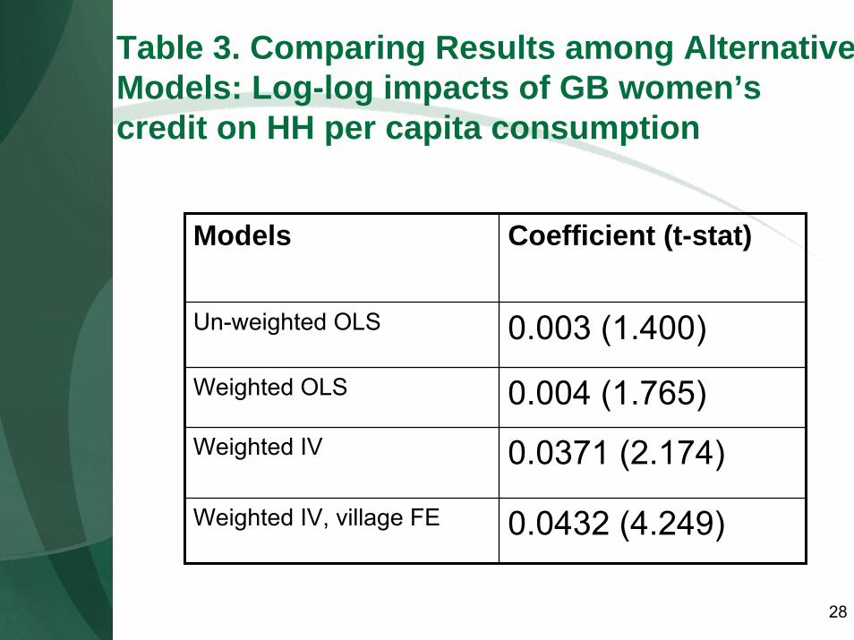
Table 3. Comparing Results among AlternativeModels: Log-log impacts of GB women’s credit on HH per capita consumption

Models Coefficient (t-stat)

Un-weighted OLS 0.003 (1.400)

Weighted OLS 0.004 (1.765)Weighted IV 0.0371 (2.174)

Weighted IV, village FE 0.0432 (4.249)

29

Conclusions

• Participants are observed to consume less on average than counterpart non-participants –does this mean program does not matter?

• Econometric estimation shows participation has indeed caused some 18 percent return to consumption for female and 11 percent for male borrowing

• IV-FE > IV > OLS

30

IV’s in Program Evaluation

• Very hard to find appropriate instrumental variables ex post

• Can build IVs into design of program

• Two Cases:– Problematic Randomization– Randomization not feasible despite best

attempts

31

IV’s in Program Evaluation• Problematic Randomization• Two Groups: Treatment (T=1) and

Control (T = 0)• Noticed

– Some people in T=1 did not get the treatment!

– Some people in T=0 did get the treatment• So, people who received the treatment

(RT for Received Treatment) is different from people chosen: RT ≠ T

• Don’t throw up hands in despair!– T is a valid IV for RT

32

IV’s in Program Evaluation• Randomization not feasible• Working with NGO to evaluate new program • Suggest quasi-experimental program design• NGO to require to follow eligibility criteria

based on observables such as landholding, gender, poverty, etc

• Construct two-groups: Z=1 and Z=0• Let NGO choose treated households

– BUT ensure more treatment samples in Z=1 than Z=0

• Use Z as instrumental variable

33

Recall classic assumption of OLS

• Assuming we can find valid IVs, we can overcome endogeneity (X is a choice variable correlated with the error):

– Simulteneity: X and Y cause each other– Omitted Variables: X is picking up the effect of

other variables– Measurement Error: X is not measured precisely

34

Caution….

• Bad instruments: if corr (Z , ε) ≠ 0, we are in trouble!– we must ensure that corr (Z , ε) = 0 – this is not always easy! We use theory and

common sense