Efficient semiparametric instrumental variable estimation 1

Feng Yao Junsen ZhangDepartment of Economics Department of EconomicsWest Virginia University The Chinese University of Hong KongMorgantown, WV 26505 USA Shatin, N.T., Hong Kongemail: feng.yao@mail.wvu.edu email: jszhang@cuhk.edu.hkVoice: + 1 304 293 7867 Voice: + 852 2609 8186

July, 2010

Abstract. We consider the estimation of a semiparametric regression model where data is inde-pendently and identically distributed. Our primary interest is on the estimation of the parametervector, where the associated regressors are correlated with the errors and contain both continuousand discrete variables. We propose three estimators by adapting Robinson’s (1988) and Li andStengos’ (1996) framework and establish their asymptotic properties. They are asymptotically nor-mally distributed and correctly centered at the true value of the parameter vector. Among a class ofsemiparametric IV estimators with conditional moment restriction, the first two are efficient underconditional homoskedasticity and the last one is efficient under heteroskedasticity. They allow thereduced form to be nonparametric, are asymptotically equivalent to semiparametric IV estimatorsthat optimally select the instrument and reach the semiparametric efficiency bounds in Chamber-lain (1992). A Monte Carlo study is performed to shed light on the finite sample properties of thesecompeting estimators. Its applicability is illustrated with an empirical data set.Keywords and Phrases. Instrumental variables, semiparametric regression, efficient estimation.

JEL Classifications. C14, C21

1We thank Carlos Martins-Filho for careful reading and constructive comments that greatly improved the paper.

We also thank Qi Li for valuable suggestions . We also receive helpful comments from seminar participates at Texas

A& M, West Virginia.

1 Introduction

There is now a vast and increasing literature on nonparametric and semiparametric estimation ofstructural models with endogenous regressors (Blundell and Powell (2001) and references). Non-parametric and semiparametric approaches relax tight parametric assumptions on the functionalforms of the structural equations or the error term distribution, thus estimation and inference arerobust to potential model misspecification.

Here, we specifically consider the literature on nonparametric and semiparametric extensionsof the classical simultaneous equations models. In these models, endogenous and predeterminedvariables are related through a system of equations, so endogeneity arises from the feedback of thedependent variable to the explanatory variable. Many recent works consider nonparametric andsemiparametric generalization of the two-stage least squares estimation to account for the endo-geneity, see Matzkin(1994, 2008), Imbens and Newey (2009) and the references cited therein foridentification and different estimation methods.

In this paper, we consider a semiparametric additive regression model

Yt = g(Z1t, Xt, εt) = m(Z1t) +Xtβ + εt, t = 1, · · · , n. (1)

We denote the endogenous explanatory variables explicitly by X′t = (Xt,1, · · · , Xt,K)′ ∈ RK , the

included exogenous variable by Z′1t = (Z1t,1, · · · , Z1t,l1)

′ ∈ Rl1 , and the excluded exogenous variableby Z′

2t ∈ Rl2 , with l1 + l2 = l. We assume the exogenous variables enter this equation of the modelvia a nonparametric function m(·), and the endogenous variables Xt influence Yt in a linear fashion.We explicitly consider continuous and discrete variables in Xt = (Xc

t , Xdt ), where Xc

t′ ∈ RKc are

the continuous variables, Xdt′ ∈ RKd discrete variables, Kc + Kc = K. Similarly Z1t = (Zc

1t, Zd1t),

Z2t = (Zc2t, Z

d2t), where Zc

1t′ ∈ Rl1c , Zc

2t′ ∈ Rl2c are the continuous variables, Zd

1t′ ∈ Rl1d and

Zd2t

′ ∈ Rl2d discrete variables.The general model of g(Z1t, Xt, εt) does not require additivity in Z1t, Xt and ε. The flexibility

is desirable in many economic applications and many results are now available ( Matzkin(1994,2008), Imbens and Newey (2009) and their references). However, identification of the parameterof interest does require further restriction on the structure of g(Z1t, Xt, ε) or the nature of theendogeneity of Xt, i.e., through the conditional distribution of εt given Xt and Zt. Many papersconsider nonparametric estimation of the structural function g(Z1t, Xt) when only εt enters themodel additively such that g(Z1t, Xt, εt) = g(Z1t, Xt) + εt, see e.g. Das (2005), Newey and Powell(1989), Dorolles et al. (2000), Newey et al. (1999), Ng and Pinkse (1995), Pinkse (2000) and Florenset al. (2008). Being robust to misspecification, the nonparametric approach is however associatedwith “curse of dimensionality” or slower convergence rate in multivariate regression. Furthermore,it is not a trivial task to incorporate both continuous and discrete variables as in Das (2005), Neweyand Powell (1989), Dorolles et al. (2000). In the control function approach considered by Newey etal. (1999), Ng and Pinkse (1995), Pinkse (2000) and Florens et al. (2008), an important assumptionis on the control variable V = X−E(X|Z). The fact that X and V are functionally related generallyrequires that endogenous components X and V be continuously distributed with unbounded support,conditionally on Z. The requirement that X is continuously distributed limits the application of thecontrol function approach.

The partially linear model in (1) provides much needed flexibility through the nonparametriccontrol function m(Z1t), while the endogenous variables Xt enter the model parametrically, allowingeasy interpretation, implementation and faster convergence rate. As a first example, consider thefixed coefficient endogenous dummy variable models of Heckman (1978), Heckman and Robb (1985),which model the impact of job training, unions status, occupational choice, schooling, the choiceof region of residence, as well as other variables on earnings. The observed outcome Yt (earnings)

1

depends on the dummy endogenous variable Xt that represents the program participation decision,and other control variables Z1t. The program participation decision is represented by a dummyvariable Xt = I(v(Zt) − ut > 0), determined by the underlying utility function v(Zt) − ut. HereI(·) is the indicator function, v(Zt) is a function of the observed characteristic vector Zt and ut

is unobserved disturbance term. β in equation (1) represents the constant impact of the program.Xt is endogenous through the correlation between u and ε. Under normality or other parametricdistributional assumptions the model can be estimated by maximum likelihood or other likelihood-based methods (for example, Heckman’s two-step estimator). It is desirable to consider distributionfree estimation of β since likelihood based methods can produce inconsistent estimators for thefixed coefficient dummy endogenous variable model if the error distribution is misspecified, see Chen(1999). At the same time, it is also desirable to allow the control functionm(Z1t) to be flexible, sincemisspecification of m(Z1t) might lead to inconsistent estimation of β as well. As a second example,consider the problem of estimating returns to schooling in Card (1993). Consider structural formestimation of an earnings model that treat experience (potential experience) as exogenous, whereYt is the log of wage, Xt is the years of schooling, and Z1t includes experience, indicators for race,southern residence, and residence in standard metropolitan statistical area. One might hesitate ininterpreting β as return to schooling since Xt is not randomly assigned or endogenous. Card usesthe proximity to a four year college as IV for education and concludes with 2SLS estimation thatOLS estimate for return to schooling might underestimate the return to schooling. Here we noticethat the control function m(Z1t) is linear. Furthermore, the reduced form of Xt is linear in theinstrumental variable and other exogenous control variables. β might be estimated inconsistently ifm(Z1t) is misspecified, and the estimation might be inefficient if reduced form is not linear.

The semiparametric regression model in (1) without endogenous variables is familiar in the liter-ature, see Robinson (1988) and Speckman (1988) under i.i.d. assumption with continuous regressors,Delgado and Mora (1995) for discrete regressor and weaker conditions than those in Robinson (1988).Theoretical results on semiparametric estimation without endogenous variables are available for de-pendent data, see Aneiros and Quintela (2001), Aneiros-Perez and Quintela-del-Rio (2002), and themonograph on partially linear models by Hardle, Liang and Gao (2000).

With endogenous variables, the precision of the estimators for β is a concern, since the restrictionimposed on m(Z1t) and on the reduced form E(Xt|Zt) are so weak. Newey (1990, 1993) consider ef-ficient estimation of a parametrically specified structural model with conditional moment restriction,see also Rilstone (1992). Newey proposes efficient estimation under conditional homoskedasticityusing nearest neighbor and series estimators. Under conditional heteroskedasiticity, Newey (1993)’sestimator reaches the semiparametric efficiency bound. However, the structural model is only para-metric. Ai and Chen (2003) consider a more general semiparametric model with conditional momentrestriction, where sieve estimation is employed and the parametric component estimator reaches thesemiparametric efficiency bound. There are relatively fewer results on dependent data semiparamet-ric instrumental variable estimation. Li and Stengos (1996), Li and Ullah (1998), Berg et al. (2000),Baltagi and Li (2002) consider the instrumental variable estimation of semiparametric dynamic paneldata model. They consider efficient estimation with non iid data.

In this paper we consider the semiparametric instrumental variable regression model in (1). Weexplicitly allow the endogenous and exogenous variables to be discrete or continuous and focuson iid data for simplicity and applicability in the cross sectional data analysis. The structuralfunction characterized by β and m(·) are easily identified with the assumptions. We propose threeestimators for β and obtain their asymptotic properties. They are shown to be consistent andasymptotically normally distributed. In a class of semiparametric IV estimators with conditionalmoment restriction, the first two are efficient under conditional homoskedasticity and are robustunder heteroskedasticity. The last estimator is efficient under heteroskedasticity. They all allow the

2

reduced form or E(Xt|Zt) to be nonparametric and are asymptotically equivalent to semiparametricIV estimators that optimally select instrument. We further show they reach the semiparametricefficiency bounds in Chamberlain (1992).

Besides the introduction, we introduce the semiparametric model and propose three estimators insection 2, provide the asymptotic properties in section 3, perform a Monte Carlo study to investigatethe finite sample performance of the estimators and to compare with other alternatives in section 4,illustrate the empirical applicability of the estimators in section 5 and conclude in section 6.

2 Semiparametric Model

Consider model (1) and assume the existence of instrumental variables Zt = (Z1t, Z2t) withE(εt|Zt) =E(εt|Z1t) = 0, for all t. To motivate the estimation, suppose we know the true conditional expecta-tion E(Yt|Z1t) = m(Z1t) + E(Xt|Z1t)β. So we could subtract E(Yt|Z1t) from (1) to obtain

Yt −E(Yt|Z1t) = (Xt −E(Xt|Z1t))β + εt. (2)

The conditional expectations are generally unknown, but we could replace them with nonpara-metric conditional mean estimators E(Yt|Z1t) and E(Xt|Z1t). However, due to correlation betweenε and X, we can not apply Robinson’s estimator by regressing Yt − E(Yt|Z1t) on Xt − E(Xt|Z1t).

Following Davidson and MacKinnon (2004) and adapting to the current notation, we couldestimate β by

β = (Q′X)−1Q′Y .

using the instrument variables Q = Q′1, Q

′2, · · · , Q′

n′if Q′t ∈ <K and Qt contain Z1t, Z2t. Here

X =

X1 − E(X1 |Z11)· · ·

Xn − E(Xn |Z1n)

, Y =

Y1 − E(Y1|Z11)· · ·

Yn − E(Yn|Z1n)

.

Li and Stengos (1996)’s estimator sets Qt = Z2t − E(Z2t|Z1t) in handling the endogeneity in thepartially linear panel data models. In the case that Qt ∈ <K+q for some positive integer q, inspiredby (8.29) in Davidson and MacKinnon, we consider the estimator of the form

β = (X′Q(Q′Q)−1Q′X)−1X′Q(Q′Q)−1Q′Y .

Estimators considered in Baltagi and Li (2002), Berg et al. (2000), Li and Ullah (1998) are inspirit similar to β using Qt = Z2t − E(Z2t|Z1t), Qt = Z2t or some other variables in the subspaces(Z) spanned by the columns of Z = (Z′

1, Z′2, · · · , Z′

n)′, where Zt = (Z1t, Z2t). As noted in Baltagiand Li (2002), setting Qt = Z2t − E(Z2t|Z1t) is equivalent to using Qt = Z2t since E(Z2t|Z1t) isorthogonal to Xt −E(Xt|Z1t). The above cited papers investigate the partially linear panel data ordynamic panel data model and they essentially consider variables in s(Z) as instrumental variablesQ. More generally, we could utilize Zt = (Z1t, Z2t) as instrumental variables since they are bydefinition exogenous. Hence we consider

β = (X′Z(Z′Z)−1Z′X)−1X′Z(Z′Z)−1Z′Y . (3)

In (3), X is projected onto the subspace s(Z) through the projection operator Z(Z′Z)−1Z′

and Z(Z′Z)−1Z′X estimates the conditional expectation E(Xt −E(Xt|Z1t)|Zt) (in Li and Stengos’

3

estimator, one could interpret X being projected parametrically onto the subspace spanned byZ2t − E(Z2t|Z1t)n

t=1). If the conditional expectation of X given Z or the reduced form is notlinear in Z, and since conditional mean is the optimal predictor of X given Z in the mean squaresense, we expect gains in efficiency by replacing the projection Z(Z′Z)−1Z′X with a nonparametricestimate.

As indicated in Robinson (1988, p. 945), a valid instrument for Xt − E(Xt|Z1t) is a vector offunction of Zt that includes Z1t and is independent of εt, such that the covariance matrix in thelimiting distribution of the n

12 consistent estimator of β exists. One candidate for the instrument is

E(Xt|Zt) − E(Xt|Z1t), where E(Xt|Zt) is a nonparametric estimator of E(Xt|Zt). We note that itcan estimate E(Xt − E(Xt|Z1t)|Zt) consistently even if E(Xt − E(Xt|Z1t)|Zt) is not linear in Zt.When m(Z1t) is absent but Xt has a nonparametric reduced form, this estimator is similar to thosein Newey (1990, 1993) and Rilstone (1992) for nonlinear equations with known structural form butunknown reduced form. We note this approach has not been pursued formally in the literature.

The conditional expectation is generally of unknown form if the structural form of Yt and Xt

contains nonlinearities in the endogenous and/or exogenous variables of unknown form, or even if theform of nonlinearity is known but information onXt’s conditional distribution given Zt is insufficientto parameterize E(Xt|Zt). Motivated by this observation, we propose two estimators for β.

Define the density of Z1t at z10 as f1(z10), and the density of Zt at z0 f(z0). We estimate themwith the Rosenblatt density estimators with both continuous and discrete variables, and we use theNadaraya-Watson estimators for E(A|z10), and E(A|z0). They are specifically

f1(z10) =1

nhl1c

1

n∑

t=1

K1(Zc

1t − zc10

h1)I(Zd

1t = zd10).

E(A|z10) =

1

nhl1c1

∑nt=1K1(

Zc1t−zc

10

h1)I(Zd

1t = zd10)At

f1(z10)

f(z0) =1

nhl1c+l2c

2

n∑

t=1

K2(Zc

1t − zc10

h2,Zc

2t − zc20

h2)I(Zd

1t = zd10, Z

d2t = zd

20).

E(A|z0) =

1

nhl1c+l2c2

∑nt=1K2(

Zc1t−zc

10

h2,

Zc2t−zc

20

h2)I(Zd

1t = zd10, Z

d2t = zd

20)At

f(z0).

where h1 and h2 are bandwidths which go to zero as n → ∞. K1(·), K2(·), and I(·) are the kerneland indicator functions. Let

W =

W1

W2

...

Wn

=

W1,1 W1,2

... W1,K

W2,1 W2,2 · · · W2,K

· · ·...

......

Wn,1 Wn,2 · · · Wn,K

, Wt,k = E(Xt,k|Zt) − E(Xt,k|Z1t),

where Xt,k is the kth element of random vector Xt. Define Y = (Y1, · · · , Yn)′, ~Z = (Z1 , · · · , Zn)′,~Z1 = (Z11, · · · , Z1n)′ and E(Y | ~Z1) = (E(Y1|Z11), E(Y2|Z12), · · · , E(Yn|Z1n))′. We propose the firstestimator as

4

β = (W ′W )−1W ′(Y − E(Y | ~Z1)). (4)

In constructing β, we first replace the unknown in Xt − E(Xt|Z1t) by the Nadaraya-Watson es-timator E(Xt|Z1t). Then we further estimate the conditional expectation E(Xt − E(Xt|Z1t)|Zt).Geometrically, we project Xt − E(Xt|Z1t) onto M(Zt), the closed linear subspace of L2 consistingof measurable function of Zt with finite second moments. Since E(Xt|Z1t) is already in M(Zt), weonly replace Xt with its conditional expectation estimator E(Xt|Zt). So in spirit, this is like Theil’s(1953) version of two stage least square estimator for simultaneous equations.

The second estimator we consider is

β = (W ′W )−1W ′(E(Y | ~Z) − E(Y | ~Z1)). (5)

where E(Y | ~Z) = (E(Y1|Z1), E(Y2|Z2), · · · , E(Yn|Zn))′. In essence, relative to the first estimator, wefurther project Yt onto M(Zt) nonparametrically. So it is in the spirit of the traditional two stageleast square estimator by Basmann (1959).

The first two estimators are shown in next section to be consistent and asymptotically efficient inTheorems 1-3 under conditional homoskedasticity and consistent under heteroskedasticity. However,they do not exploit the structure of heteroskedasticity if it’s present. To properly account for theinformation provided by heteroskedasticity, it is important to estimate the conditional variancecorrectly. We provide our third estimator βE in two steps. To simplify the analysis, we focuson the case that heteroskedasiticity depends only on the included exogenous variables, that is,E(ε2t |Zt) = σ2(Z1t) as in A6(1) below. First, the estimated residual based on β is εt = Yt−E(Y |Z1t)−(Xt− E(X|Z1t))β. The conditional variance is nonparametrically estimated as σ2(Z1t) = E(ε2|Z1t).

The conditional covariance matrix Ω(~Z1) is estimated with Ω(~Z1), which is a diagonal matrix withthe t − th element as σ2(Z1t). Second, inspired by the generalized least squares estimator, weconstruct the feasible efficient estimator as

βE = (W ′Ω−1(~Z1)W )−1W ′Ω−1(~Z1)(E(Y | ~Z) − E(Y | ~Z1)). (6)

In some application of the kernel regression estimators, E(A|z0) and E(A|z10) could cause tech-

nical difficulty due to the random denominator f(z10) and f(z0), which could be small. We could

follow Robinson (1988), Bickel (1982) and Manski (1984) to “trim” out small f(z10) and f(z0), orreplace them with small but positive constant. We expect this will not change the asymptotic resultsso we will not introduce it in the definition. Alternatively we could follow Li and Stengos (1996)or Powell, Stock and Stoker (1989) to estimate a density-weighted relationship and we expect theasymptotic results will be different. Using an indicator function to account for the discrete variableshas been considered in other contexts by Delgado and Mora (1995), Fan et al. (1998), Camlong-Viotet al. (2006). One could also follow Racine and Li (2004) to introduce more delicated estimatorfor the discrete variables for improved finite sample performance, but in this case one does need toconsider the selection of additional smoothing parameters.

3 Asymptotic properties

As in parametric instrumental variable estimation, our semiparametric instrumental variable es-timators are likely to be biased. We investigate their asymptotic properties with the followingassumptions. We let c denote a generic constant below, which can vary from one place to another.A1: (1)Yt, Xt, Ztn

t=1 is an independent and identically distributed sequence of random vectorsrelated as in (1).

5

(2) E(εt|Zt) = 0 for all t.(3) Let Wt = E(Xt|Zt) − E(Xt|Z1t), EW

′tWt is a symmetric and positive definite matrix.

A2: (1) Denote the density of Z1t at z1 by f1(zc1, z

d1), which is s times continuously differentiable

with respect to (w.r.t.) zc1. Furthermore, the sth order derivative is uniformly continuous on Gc

1.

G1 = Gc1 ×Gd

1 ⊂ <l1 , G1 compact. We adopt the notation that j = (j1, j2, · · · , jl1c)′, |j| =

∑l1c

i=1 ji.The |j|th order partial derivative w.r.t. zc

1 is

∂j

∂(zc1)

jf1(z

c1, z

d1) ≡ ∂|j|f1(zc

1 , zd1)

∂(zc1,1)

j1∂(zc1,2)

j2 · · ·∂(zc1,l1c

)jl1c

and supz1∈G1| ∂j

∂(zc1)

j f1(zc1, z

d1)| <∞, where |j| = 1, 2, · · ·, s. For future purpose, we denote

∑

0≤|j|≤s =∑

|j|=0 +∑

|j|=1 + · · ·+∑|j|=s, j! = j1!× j2!× · · ·× jl1c!, (zc

1)j = (zc

1,1)j1 × (zc

1,2)j2 × · · ·× (zc

1,lc)jl1c .

(2) 0 < c < f1(zc1, z

d1) <∞, for all z1 ∈ G1.

(3) Xt,k = E(Xt,k|Z1t) + Xt,k − E(Xt,k|Z1t) = g1,k(Z1t) + e1,kt, ∀zd1 ∈ Gd

1, g1,k(z1) is s1 timescontinuously differentiable w.r.t. zc

1, s1 > s, with the sth and s1th order derivative uniformly

continuous on Gc1. The |j|th order derivative w.r.t. zc

1 is ∂j

∂(zc1)

j g1,k(zc1, z

d1) defined similarly as in

A2(1) and supz1∈G1| ∂j

∂(zc1)

j g1,k(zc1, z

d1)| <∞, where |j| = 1, 2, · · · , s1. The conditional density of Z1t

given e1,kt is bounded, and the conditional density of Xt,k given Z1t is continuous around Zc1t.

(4) Denote the density of Zt at z by fz(zc1 , z

d1 , z

c2, z

d2) = fz(z), which is s1 times continuously

differentiable w.r.t. zc = (zc1, z

c2) with the sth and s1th order derivative uniformly continuous on

Gc1 ×Gc

2. G = Gc1 ×Gd

1 ×Gc2 ×Gd

2 ⊂ <l, G2 = Gc2 ×Gd

2 compact. The |j|th order derivative w.r.t.zc is

∂j

∂(zc)jfz(z) ≡ ∂|j|fz(z

c1 , z

d1 , z

c2, z

d2)

∂(zc1,1)

j1∂(zc1,2)

j2 · · ·∂(zc1,l1c

)jl1c∂(zc2,1)

jl1c+1∂(zc2,2)

jl1c+2 · · ·∂(zc2,l2c

)jl1c+l2c

and supz∈G | ∂j

∂(zc)j fz(zc1, z

d1 , z

c2, z

d2)| <∞, where |j| = 1, 2, · · · , s1.

(5) 0 < c < fz(z) <∞, for all z ∈ G.(6) Xt,k = E(Xt,k|Zt)+Xt,k−E(Xt,k|Zt) = gk(Zt)+ekt, gk(z) is s1 times continuously differentiablew.r.t. zc = (zc

1, zc2), s1 ≥ s, with the sth and s1th order derivative uniformly continuous on Gc

1 ×Gc

2. The |j|th order derivative w.r.t. zc is ∂j

∂(zc)j gk(zc, zd) defined similarly as in A2(4) and and

supz∈G | ∂j

∂(zc)j gk(zc, zd)| < ∞, where |j| = 1, 2, · · · , s1. The conditional density of Zt given ekt is

bounded, and the conditional density of Xt,k given Zt is continuous around Zct .

(7) m(z1) is s1 times continuously differentiable w.r.t. zc1 with its sth and s1th order derivative

uniformly continuous on Gc1. We denote the |j|th order derivative as ∂j

∂(zc1)

j m(z1), defined similarly

as in A2(1) and supz1∈G1| ∂j

∂(zc1)

j m(z1)| <∞, where |j| = 1, 2, · · · , s1.A3: (1) For x ∈ <d, d = l1c or l2c, the kernel function K(x)(K1(x) or K2(x)) is bounded withbounded support, and it is of order 3s1.(2) |uiK(u) − viK(v)| ≤ Ck||u− v||, |i| = 0, 1, 2, · · · , s1.A4: (1) For some δ > 0, E(X2+δ

t,k |Zt), E(X2+δt,k |Z1t) <∞,

|gk(Zt)|, |g1,k(Z1t)| <∞ almost everywhere.(2) E(ε2+δ

t |Zt), E(ε2+δt |Z1t) <∞.

(3) E(ε2t |Zt) = σ2(Zt).(4) The conditional density of Z1t given εt is bounded, and the conditional density of εt given Z1t

is continuous around Zc1t. The conditional density of Zt given εt is bounded, and the conditional

density of εt given Zt is continuous around Zct .

6

A5: (1) nh2l1c

1 → ∞. (2) nh2(l1c+l2c)2 → ∞. (3) nh

2(s+1)1 , nh

2(s1+1)2 → 0.

A6: (1) E(ε2t |Zt) = E(ε2t |Z1t) = σ2(Z1t). 0 < c < σ2(Z1t) < ∞, σ2(Z1t) is s1 times contin-uously differentiable w.r.t. zc

1 with its sth and s1th order derivative uniformly continuous on

Gc1. We denote the |j|th order derivative as ∂j

∂(zc1)

j σ2(Z1t), defined similarly as in A2(1) and

supz1∈G1| ∂j

∂(zc1)j σ

2(Z1t)| <∞, where |j| = 1, 2, · · · , s1.(2) E( 1

σ2(Z1t)W ′

tWt) is a symmetric and positive definite matrix.

(3) E(X4+δt,k |Z1t) <∞, E(X2

t,k|Z1t) is uniformly continuous at Zc1t and E(ε4+δ

t |Z1t) <∞.

A7: (1) E(X4t,k|Zt) <∞. (2) E(ε4t |Zt) <∞. (3) σ2(Z1t) is continuous at Zc

1t.

Note that in A1(2), we require the conditional expectation of the error term εt given Zt to bezero, but we allow εt’s and Xt’s to be possibly correlated, thus Zt play the role of instrumentalvariables. A1(3) is the identification assumption for β, similar to the identification assumption inRobinson (1988). From equation (1) and A1(2),

E(Yt|Zt) −E(Yt|Z1t) = [E(Xt|Zt) − E(Xt|Z1t)]β = Wtβ

So we pre-multiply both sides by W ′t and take expectation, we have with A1(3)

E(W ′t (E(Yt|Zt) − E(Yt|Z1t))) = E(W ′

tWt)β

⇒ β = (EW ′tWt)

−1E(W ′t (E(Yt|Zt) −E(Yt|Z1t))).

Since conditional expectations are identified, β is identified with A1(3). First, X can’t containconstant. Second, it implies that E(X|Z) 6= E(X|Z1). Since Z = (Z1, Z2), any element of X can’tbe perfectly a.s. predictable by Z1, i.e., X can’t be some function of Z1 only. Obviously Z2 can’t besimply linear combination of Z1, so Z2 need to contain variables that are linearly independent of Z1.A1(3) forbids more general forms of dependence. Third, since Wt can’t be a.s. zero, no elements ofE(X|Z) − E(X|Z1) are multicollinear. This fails if X is collinear.

Assumption A2(1),(2),(4),(5),(7) require the densities f1(z1), fz(z) and m(z1) to be continuouslydifferentiable w.r.t. its continuous components and bounded. These assumptions are commonly usedin nonparametric kernel regression, enabling the use of Taylor expansion (Martins-Filho and Yao(2007)). They are similar in spirit to the smoothness and boundedness condition in Definition 2 ofRobinson (1988), or assumption A1 of Li and Stengos (1996). A2(3) and (6) explicitly assume therelationship between Xt and Z1t and between Xt and Zt. Similar assumptions have been maintainedin Aneiros and Quintela (2001) and Speckman (1988) in the fixed design case. Assumption A3 re-quires the kernel function to be smooth and bounded (Martins-Filho and Yao (2007)). Asymptoticdistributions are established using Liapunov’s central limit theorem, with conditional moments as-sumption of εt and Xt given Zt or Z1t in A4. The bandwidth assumptions A5(1) and (2) are in linewith those used in the literature (Martins-Filho and Yao (2007)). A3 together with A5(3) specifiesthe kernel properties and the rate of decay for the bandwidths. They are used to control the bias in-troduced in the nonparametric regression, which is similar to assumptions, for example, in Robinson(1988), Li and Stengos (1996). However, A5(3) is stronger than those maintained in Li and Stengos,Li and Ullah or Robinson. As our estimators involve estimation of Wt, the bias arises not only fromestimation of E(Xt|Z1t), but also from estimation of E(Xt|Zt). A5 requires choice of higher orderkernel to eliminate the bias asymptotically. Results in Theorem 1-3 are obtained for general het-eroskedasticity structure in A4(3). For efficient estimation, we restrict the structure of E(ε2t |Zt) tobe σ2(Z1t) in A6(1) for simplicity, so the heteroskedasticity depends only on the included exogenous

7

variables. Assumption A6 provides higher moments and additional smoothness conditions, enablingus to obtain the asymptotic results for βE , which involves estimation of the conditional covariancematrix of ε. The asymptotic results for β are obtained with additional moments conditions in A7.Theorem 1 Let Φ0 be a K×K positive definite matrix with the (i, j)th element E[σ2(Zt)(gi(Zt)−EZ2τ |Z1t

(gi(Z1t, Z2τ)))(gj(Zt) − EZ2τ |Z1t(gj(Z1t, Z2τ )))], where EZ2τ |Z1t

(.) denotes the conditionalexpectation of Z2τ given Z1t. With assumption A1-A5, we have

√n(β − β)

d→ N(0, (EW ′tWt)

−1Φ0(EW′tWt)

−1)

β is relatively easier to construct as it does not involve further projecting Yt onto M(Zt) andis in spirit like Theil’s two stage least square estimator. But we notice that Wt,k estimate Wt

nonparametrically, so the simplicity in Theil’s original estimator disappears. In finite samples, βas well as β are not unbiased. Furthermore, compared to β, we find in Theorem 2’s proof that theasymptotic expansion of β−β involves more stochastic terms, whose magnitudes need to be furthercontrolled to obtain the asymptotic distribution. However, we do find the asymptotic distributionof β to be the same as that of β. The finite sample performance of the two proposed estimators isinvestigated in the simulation section and it indicates β always outperforms β.Theorem 2 Let Φ0 be defined in Theorem 1. With assumption A1-A5 and A7, we have

√n(β − β)

d→ N(0, (EW ′tWt)

−1Φ0(EW′tWt)

−1)

From Theorem 1 and 2, we note β and β are consistent and asymptotically normal with gen-eral conditional variance structure specified in A4(3). When ε is conditionally homoskedastic, i.e.,V (εt|Zt) = σ2

0 , it is straightforward to compare the asymptotic properties of the proposed estimatorswith β, since they are consistent and all converge to a normal distribution at rate

√n. We find the

asymptotic variance of β is always greater or equal to that of the two proposed estimators, i.e., thedifference is a positive semidefinite matrix. So β and β are asymptotically efficient relative to β.Theorem 3 If V (εt|Zt) = σ2

0, then the asymptotic variance of β is greater than or equal to that of

β or β.To illustrate the point, we first observe in Φ0,

EZ2τ |Z1t(gj(Z1t, Z2τ)) = EZ2τ |Z1t

(E(Xt,j |(Z1t, Z2τ))) = E(Xt,j |Z1t).

So (EW ′tWt)

−1Φ0(EW′tWt)

−1 = σ20(EW

′tWt)

−1. For the estimator β defined in equation (3), supposethe estimated items are replaced by the true values, we obtain with equation (2),

βTr = ((XTr)′ ~Z(~Z′ ~Z)−1 ~Z′XTr)−1(XTr)′ ~Z(~Z′ ~Z)−1 ~Z′Y Tr

= β + ((XTr)′ ~Z(~Z′ ~Z)−1 ~Z′XTr)−1(XTr)′ ~Z(~Z′ ~Z)−1 ~Z′~ε

where XTr = Xt − E(Xt|Z1t)nt=1, Y

Tr = Yt − E(Yt|Z1t)nt=1, and ~ε = εtn

t=1. We expect theasymptotic distribution of β to be the same as that of βTr , if the unknown conditional expectations

are estimated with nonparametric kernel estimates. Suppose that 1nZ′~ε

p→ 0, which follows from

the assumption of Z being instrumental variables. Assume further that 1n ((XTr)′Z)

p→ E[(Xt −E(Xt|Z1t))

′Zt] = A, and 1nZ

′Zp→ E(Z′

tZt) = B, A has rank K and B is positive definite. We have1nV (~Z′~ε) = σ2

0B, since ε is conditionally homoskedastic. Then we expect

√n(βTr − β)

d→ N(0, σ20(AB

−1A′)−1).

The theorem is proved if σ20(AB

−1A′)−1 − σ20(EW

′tWt)

−1 is positive semidefinite.

8

Above claim is equivalent to EW ′tWt − AB−1A′ being positive semidefinite. We note

A = E[(Xt −E(Xt|Z1t))′Zt] = E[(E(X′

t|Zt) − E(X′t|Z1t))Zt] = E(W ′

tZt)

So EW ′tWt −AB−1A′ = E(W ′

tWt) −E(W ′tZt)(EZ

′tZt)

−1E(Z′tWt)

= E[W ′t(Wt − Zt(EZ

′tZt)

−1E(Z′tWt))]

= E[(Wt − Zt(EZ′tZt)

−1E(Z′tWt))

′(Wt − Zt(EZ′tZt)

−1E(Z′tWt))]

which is positive semidefinite. The last equality is true as

E[(Zt(E(Z′tZt))

−1E(Z′tWt))

′(Wt − Zt(E(Z′tZt))

−1E(Z′tWt))]

= E(W ′tZt)(E(Z′

tZt))−1E(Z′

tWt)−E(W ′

tZt)(E(Z′tZt))

−1E(Z′tZt)(E(Z′

tZt))−1E(Z′

tWt)= 0.

When ε is conditionally heteroskedastic as in A6(1), we consider the feasible estimator βE , which

is based on first stage estimation with β. We did not consider β since it’s outperformed by β in thesimulation study in section 4. The asymptotic property of βE is provided in Theorem 4.Theorem 4 If we assume A1-A6, then

√n(βE − β)

d→ N(0, (E1

σ2(Z1t)W ′

tWt)−1).

To shed light on the theoretical results above, let’s consider a class of semiparametric IV es-timators based on model (1) that satisfy the conditional moment restriction E(εt|Zt) = 0, where

εt = εt(β) = Yt −E(Yt|Z1t) − (Xt −E(Xt|Z1t))β as in (2). Then β and β are asymptotically equiv-alent to the semiparametric IV estimator that optimally selects instrument variables. Thus β andβ are efficient among this class of semiparametric IV estiamtors in the sense that their asymptoticvariance is smallest. To see this, suppose E(Yt|Z1t) and E(Xt|Z1t) are known, or can be consistentlyestimated at certain rate, then let H(Zt) denote a h× 1 vector of functions of Zt, h ≥ K. By law ofiterated expectation we have E(H(Zt)εt(β)) = 0. Following Newey (1993), we could construct theIV estimators using the method of moments estimator. It is defined as

βMIV = argminβ gn(β)′P gn(β), gn(β) =1

n

n∑

t=1

H(Zt)εt(β),

for h×h positive semidefinite matrix P , which may be random. Since εt(β) is linear in β, by solvingthe minimization problem we easily obtain,

√n(βMIV − β) = [ 1

n

∑

t(Xt − E(Xt|Z1t))′H(Zt)

′P 1n

∑

t H(Zt)(Xt − E(Xt|Z1t))]−1

× 1n

∑

t(Xt −E(Xt|Z1t))′H(Zt)

′P√n 1

n

∑

t H(Zt)εt,

Assume Pp→ P , P positive semi-definite, 1

n

∑

t H(Zt)(Xt −E(Xt|Z1t))p→ −E(H(Zt)

∂εt(β)∂β

) = −Gand define V = EH(Zt)εtε

′tH(Zt)

′ = Eσ2(Zt)H(Zt)H(Zt)′, then

√n(βMIV − β)

d→ N(0, (G′PG)−1G′PV P ′G(G′PG)−1),

9

Under conditional homoskedasticity, σ2(Zt) = σ2, so the asymptotic variance of β is σ2(EW ′tWt)

−1.

Let A = G′PH(Zt)εt(β), B = −[E(Xt −E(Xt|Z1t)|Zt)]′ εt(β)

σ2 , then

(G′PG)−1G′PV P ′G(G′PG)−1) − σ2(EW ′tWt)

−1

= E(EAB′)−1[A− (EAB′)(EBB′)−1B][A′ − B′(EBB′)−1(EBA′)](EBA′)−1

which is a quadratic form, so the difference is positive semidefinite. We note the asymptotic vari-

ances will be the same if we let the optimal instrumental variable to be H(Zt) = −W ′t

σ2 . So asymp-

totically, β and β behave like an optimal semiparametric IV estimator. Under conditional het-eroskedasticity specified in A6(1), we could follow similar argument above to show the differencebetween (G′PG)−1G′PV P ′G(G′PG)−1 and (E 1

σ2(Z1t)W ′

tWt)−1) is positive semidefinite. Here the

two asymptotic variances will be the same if we let H(Zt) = − W ′t

σ2(Z1t), so asymptotically βE behaves

similarly as an optimal semiparametric IV estimator under heteroskedasticity.We further compare the theoretical results in Theorem 1-4 with the semiparametric efficiency

bound derived in Chamberlain (1992). Our model (1) and assumption A1(2) consider the estimationof β in model of εt = Yt−m(Z1t)−Xtβ with the conditional moment restriction E(εt|Zt) = 0. Since∂ε∂β′ = −X, define D0(Z) ≡ E( ∂ε

∂β′ |Z) = −E(X|Z),Σ0(Z) ≡ E(εε′|Z) = σ2(Z), H0(Z) ≡ E( ∂ε∂r |Z) =

−1 for r = m(x). The Fisher information bound for β is

J0 = EE(D′0Σ

−10 D0|Z1) −E(D′

0Σ−10 H0|Z1)[E(H ′

0Σ−10 H0|Z1)]

−1E(H ′0Σ

−10 D0|Z1).

It is easy to show that under homoskedasticity Σ0(Z) = σ2 and

J0 =1

σ2EW ′

tWt = [(EW ′tWt)

−1Φ0(EW′tWt)

−1]−1

as in Theorem 1 and 2. Under the heteroskedasticiy structure imposed in A4(3), Σ0(Z) = σ2(Z1),

we have J0 = E( 1σ2(Z1t)

W ′tWt), as in Theorem 4. So we conclude the estimators β, β and βE reach

the semiparametric efficiency bound.

4 Monte Carlo Study

In this section, we perform a Monte Carlo study to implement our efficient semiparametric instru-mental variable estimators and illustrate their finite sample performance. For ease of comparison,we consider the data generating process in Baltagi and Li (2002) adapted to the iid set up as

Yt = βXt + α1Z1t + α2Z21t + εt, and Xt = gi(Z1t, Z2t) + Ut.

Here the nonlinear function m(Z1t) is α1Z1t + α2Z21t and we fix β = α1 = α2 = 1. We generate Z1t

and Z2t independently from a standard normal distribution, truncated to [−1, 1]. Conditional onZt, εt and Ut are generated from a bivariate normal distribution with zero mean, variance σ2

i (Zt),and correlation θ. We truncate εt and Ut to [−1, 1] × [−1, 1]. We consider σ2

1(Zt) = 1 for thehomoskedasticity case, and σ2

2(Zt) = Z21t for the heteroskedasticity case. We choose θ = 0.2, 0.5, 0.8.

As θ increases, the correlation between Xt and εt increases, thus endogeneity is magnified. Weselect two functions for gi, with g1(Z1t, Z2t) = γ1Z1t + γ2Z2t and g2(Z1t, Z2t) = γ1Z

21t + γ2Z

22t, with

γ1 = γ2 = 1. So with g1, Xt depends on Zt linearly, while in g2, Xt relates to Zt in a nonlinearfashion. It is easy to verify that assumptions maintained in A1, A2 and A4 are satisfied. We considertwo sample sizes n = 100 and 200 and perform 1000 repetitions for each experimental design.

10

To implement our estimators β, β and βE , we need to select the bandwidth sequences h1 andh2. We select the bandwidth h1 using the rule-of-thumb data driven plug-in method of Ruppert,Sheather and Wand (1995). We select h2 using 1.25SD(Zt)n

−1/6, where SD(Zt) is the standarddeviation of Zt. We choose a second order Epanechnikov kernel, which satisfies our assumption A3.With the choice of bandwidth and kernel, our assumption A5 is violated. So we investigate therobustness of our estimators against popular kernel function with lower order. From our asymptoticanalysis in Theorem 1 and 2 as well as the comments before Theorem 1, β and β might have higherfinite sample bias.

Besides the two estimators we proposed, we also include the semiparametric estimator β1 withoutconsidering the endogenous variable as in Robinson, estimator β2 as in Li and Stengos with instru-mental variable Qt = Z2t− E(Z2t|Z1t) using the density weighted estimation, and β in equation (3).β1 serves as the benchmark since it ignores the endogeneity problem. We evaluate the performanceof each estimator using bias (B), standard deviation (S) and root mean squared error (R) as criteria.The results of the experiments with σ2

1(Zt) = 1 are summarized in Table 1 for g1 and Table 2 forg2, and the results with σ2

2(Zt) = Z21t are provided in Table 3 and 4.

We observe that β and β2 generally has negative bias under g1, while other estimators producepositive bias. As sample size n increases, the estimators’ performance generally improve in terms ofsmaller bias, standard deviation and root mean squared error. This observation is consistent withour asymptotic results in Theorem 1, 2 and 4 that β, β and βE are consistent. Exceptions occurwith β1 whose bias does not seem to drop with large sample. Exceptions also exist with β2 and βin data generating process g2. This observation is consistent with the fact that in g2, E(Xt|Zt) isnot linear in Zt, while β2 and β implicitly assume E(Xt|Zt) is linear in Zt.

As θ increases, the endogeneity problem is magnified. β1’s bias increases. Though its standarddeviation drops slightly, the drop in standard deviation is dominated by the increase in bias, andthe root mean squared error also increases. This is expected since β1 does not take endogeneityinto consideration. We notice the bias of all estimators generally increase with θ. For β and βE

in the homoskedasticity experiments, their standard deviation drop with θ, though their root meansquared error increase.

When g1 is in the data generating process and homoskedasticity is present, we note E(Xt|Zt)is linear in Zt. In terms of relative performance, β1 carries the largest bias, smallest standarddeviation. As expected, its root mean squared error is largest with θ = 0.5 or 0.8. Among the restestimators that take endogeneity into account, β2’s or β’s bias is smallest, followed by β, by βE andby β. The relatively large bias of β, βE and β might be explained as we use a second order kernelfunction which violates our assumption A5, while it is permitted in Li and Stengos. However, β isthe best using standard deviation as criterion, followed by βE and β which is better for large θ orby β, while β2 carries the largest standard deviation. This result is consistent with our Theorem 3,which indicates the asymptotic variance of β, βE and β is smaller than or equal to β. Though withthe same asymptotic distribution, β’s standard deviation is larger than β’s. This is consistent withour observation before Theorem 2. The asymptotic expansion of β−β involves additional stochasticterms. Though their magnitudes are controlled asymptotically, their presence does influence thefinite sample performance. β’s performance is generally best in terms of root mean squared error,followed by β and βE , by β2 and β, with exceptions at θ = 0.2 where β performs best. β’s goodperformance is expected since with g1, β correctly assumes E(Xt|Zt) to be linear in Zt. Whenthe heteroskedasticity assumption is in place, we notice the best estimator is βE in terms of bias,standard deviation and root mean squared error. The reduction of standard deviation relative to βis well over 10%. The conclusion we draw for the performance of the rest estimators is similar to thatin the homoskedasticity case, except we notice β2 performs much better, outperformed only by βE atleast in terms of root mean squared error. Since βE properly take into account the heteroskedasticity

11

structure, the observation confirms our theoretical result in previous section that βE reaches thesemiparametric efficiency bound.

When g2 and homoskedasticity are in the data generating process, we note E(Xt|Zt) is notlinear in Zt. β1 carries the smallest standard deviation with relatively large bias, while its rootmean squared error is generally larger than β, βE and β. Among the rest estimators, β, βE and βare the best in terms of small bias and standard deviation, especially when the endogeneity problemis more severe. It is quite obvious that β has the smallest root mean squared error. βE performssimilarly well, followed by β. β2 and β are outperformed by the others, due to the fact that E(Xt|Zt)is not linear in the data generating process. This again confirms our results in Theorem 3. When theheteroskedasticity situation is considered, we notice again, βE performs best among all estimators.The comments about the other estimators in the homoskedasticity case continue to be valid.

To summarize, under homoskedasticity, we conclude that when E(Xt|Zt) is linear in Zt, allestimators taking endogeneity into account perform better than β1. β is the best in this case with β,βE and β2 being competitive alternatives. When E(Xt|Zt) is not linear in Zt, estimators β, βE and βperform best, since they estimate E(Xt|Zt) nonparametrically, avoiding potential misspecification.

We generally recommend the use of β over β due to better finite sample performance. Underheteroskedasticity, however, the best estimator is βE , which properly accounts for the informationin the variance structure. β continues to be a competitive alternative, though less efficient.

5 Empirical Illustration

We illustrate the applicability of our proposed estimators using the return to schooling data setfrom Card (1995). Using 3010 observations from the National Longitudinal Survey of Young Menin 1976, Card considers the regression model

logwage = β0 +β1educ +β2exper +β3exper2

OLS 0.074 0.084 −0.2242SLS 0.132 0.107 −0.228

+β4black +β5south +β6smsa + ε−0.190 −0.125 0.161−0.131 −0.105 0.131

where logwage is the log of 1976 hourly wage in cents, educ is years of schooling, exper is thepotential experience constructed as age−educ−6. black, south, and smsa (Standard MetropolitanStatistical Area) are dummy variables, see Card for detailed data description and analysis. TheOLS estimate for β1 is 0.074 with standard error of 0.004, however, due to the fact that educ isnot randomly assigned or endogenous, it is hard to argue it to be the return to schooling. Carduses the proximity to a four year college as an instrumental variable for educ. Since being locatedclose to a college might reduce the cost of investing in education, one might get more education.The 2SLS estimate for β1 is 0.132 with standard error of 0.049. Thus the return to schooling mightbe underestimated in OLS, even though OLS estimate carries a much smaller standard error. Wenotice the specification might be restrictive, i.e., experience enters the control function as a quadraticfunction and the dummy variables carry fixed coefficients. The larger value of β1 in 2SLS might bedue to the restrictive control function form. So we consider semiparametric estimation of β in themodel

logwage = βeduc +m(exper, black, south, smsa) + residuals

12

using the two estimators proposed in the paper, β and β. Since the 2SLS results reported in Card arequite stable for treating experience as either exogenous or endogenous, we simply treat experienceas exogenous variable for illustration purpose. We adopt the proximity to a four year college as theIV for educ and choose the kernel function and bandwidths as in the Monte Carlo study. When βis used, one can construct estimate for m(·) as

m(Z1t) = E(Y |Z1t) − E(X|Z1t)β

The estimated residual is εt = Yt −Xtβ− m(Z1t). Based on our Theorem 1, we can easily estimatethe variance for β as (W ′W )−1 1

n

∑nt=1 ε

2t , if ε is conditionally homoskedastic. If not, the heterosked-

asiticity consistent variance estimate is constructed as (W ′W )−1W ΩW ′(W ′W )−1 following White(1980), where Ω is a diagonal matrix with ε2t as its diagonal term. Similar estimate could be obtained

for the variance of β as well using Theorem 2.We obtain β = 0.048 with standard error of 0.019, and β = 0.091 with standard error of 0.019.

The heteroskedasticity robust standard error is 0.016 for both estimates. It suggests that the returnto schooling obtained in 2SLS might be too big, due to its restrictive control function form. To furtherillustrate the difference, we provide the estimated m(exper, black, south, smsa) using β in Figure1 for all combinations of the race and location status, except for (black, south, smsa) = (1, 0, 0)which has only 5 occurences in the sample. The estimated control function using 2SLS is alsoprovided in Figure 2 for comparison purpose. Figure 2 shows all m(·) are quadratic functionswith different intercepts, with the difference between each of the two m(·)′s being fixed. On theother hand, Figure 1 gives quite different estimation results. For example, the quadratic controlfunction assumption might be reasonable for a non-black person in the northern metropolitan area( (black, south, smsa) = (0, 0, 1)), but it is unlikely to be the case for a black person located in thesouthern non-metropolitan area ( (black, south, smsa) = (1, 1, 0)). The gap between their expectedincome is indeed largest as in Figure 2, but the gap changes across different experience. Furthermore,the intercepts of m(·) in Figure 1 are higher than those in Figure 2, which follows since β estimateis smaller. To get an overall picture of the difference of two estimation procedures (semiparametricIV with β and 2SLS) in capturing logwage, we plot the predicted logwage against the realizedlogwage. A solid line is superimposed to indicate perfect prediction. Both estimates seem tooverestimate logwage when it is small, but underestimate logwage when it is large. Furthermore,semiparametic IV estimates’s variability seems to be smaller.

Since the potential experience is closely related to the education, exper might be endogenousfor the same reason that education is endogenous. To check the robustness of above findings, weconsider the alternative model as

logwage = βeduc+m(age, black, south, smsa) + residuals,

which replaces exper in the control function by age. We repeat the semiparametric IV estimationprocedures with proximity to four-year college as IV for educ. We obtain β = 0.024 with standarderror of 0.019, and β = 0.039 with standard error of 0.019. The heteroskedasticity robust standarderror is 0.017 for both estimates. Though the estimates change, we still conclude that 2SLS estimatefor return to schooling might be too big.

6 Conclusion

In this paper we consider the efficient estimation of a semiparametric regression model where the en-dogenous variables enter parametrically. We allow the endogenous as well as the exogenous variables

13

to be either discrete or continuous. We propose three estimators for the parametric parameters andwe show they are consistent and asymptotically normal. The first two estimators are efficient relativeto previously considered estimators under homoskedasticity and are consistent under heteroskedas-ticity. The third estimator incorporates the potential heteroskedasticity information into estimation,and is more efficient under heteroskedasticity. They allow the reduced form to be nonparametric andare asymptotically equivalent to semiparametric IV estimators that optimally select the instrumentunder conditional moment restriction. They reach the semiparametric efficiency bounds in Cham-berlain (1992). We investigate the finite sample performance in a Monte Carlo study and illustrateits empirical applicability using the return to schooling data in Card (1993).

Appendix 1

Lemma 1 Define

Sn,j(z0) =1

n

n∑

i=1

Kh(Zci − zc

0)

(Zc

i − zc0

h

)j

I(Zdi = zd

0)g(Ui)w(Zci − zc

0; z0), |j| = 0, 1, · · · , J,

where Zi, Ui are iid, Zci ∈ Rlc , Zd

i ∈ Rld , Kh(·) = 1hlcK( ·

h ), and K(·) is a kernel function defined

on Rlc . Here similar to notations in A2(1), j = (j1, j2, · · · , jlc), Zci = (Zc

i,1, Zci,2, · · · , Zc

i,lc), zc

0 =

(zc0,1, z

c0,2, · · · , zc

0,lc), and

(Zc

i −zc0

h

)j

=(

Zci,1−zc

0,1

h

)j1× · · · ×

(Zc

i,lc−zc

0,lc

h

)jlc

. Assume

L1. K(.) is bounded with compact support and for Euclidean norm ||.||,

|ujK(u) − vjK(v)| ≤ cK ||u− v||, for 0 ≤ |j| ≤ J.

L2. g(Ui) is a measurable function of Ui and E|g(Ui)|s <∞ for s > 2.L3. For G a compact subset of <lc+ld , define the joint density of Zi and Ui at (z0 , u) as f(z0 , u),conditional density of Zi and Ui given Ui at Zi = z0 and Ui = u as fz|u(z0). Assumesupz0∈G

∫|g(u)|sfz,u(z0 , u)du <∞, fz|u(z0) <∞, and fz,u(z0, u) is continuous around zc

0.

L4. w(Zci − zc

0; z0) is a function of Zci − zc

0 and z0. |w(Zci − zc

0; z0)| < c <∞, |w(Zci − zc

0; zc0, z

d0) −

w(Zci − zc

k; zck, z

d0)| ≤ c||zc

0 − zck|| almost everywhere.

L5. nhlc → ∞.

Then for z0 = (zc0, z

d0) ∈ G = Gc ×Gd, Gc and Gd compact subsets of Rlc and Rld respectively,

supz0∈G

|Sn,j(z0) −E(Sn,j(z0))| = Op

((nhlc

ln(n)

)− 12

)

.

Proof. Let’s define

SBn,j(z0) =

1

n

n∑

i=1

Kh(Zci − zc

0)

(Zc

i − zc0

h

)j

I(Zdi = zd

0 )g(Ui)w(Zci − zc

0; z0)I(|g(Ui)| ≤ Bn),

where B1 ≤ B2 ≤ · · · such that∑∞

i=1 B−si < ∞ for some s > 0. Since Gc × Gd is compact, we

could cover G by a finite number ln of lc dimensional cubes Ik with center zk, k = 1, 2, · · · , ln andlength rn. We could choose ln sufficiently large such that rn is sufficiently small and each cube Ikcorresponds to one fixed possible value of zd

0 , i.e., zd0 = zd

k if z0 ∈ Ik. Since G is compact, lnrlcn = c,

c a constant. Suppose we let ln =(

nln(n)hlc+2

) lc2

, then rn = c/l1lcn . Since

14

supz0∈G |SBn,j(z0) −E(SB

n,j(z0))|= max1≤k≤ln supz0∈Ik∩G |SB

n,j(z0) −E(SBn,j(z0))|

= max1≤k≤ln supz0∈Ik∩G |SBn,j(z

c0 , z

dk) −E(SB

n,j(zc0, z

dk))|

= max1≤k≤ln supzc0∈Ik∩Gc |SB

n,j(zc0, z

dk) − SB

n,j(zk)

+SBn,j(zk) −ESB

n,j(zk) +ESBn,j(zk) −ESB

n,j(zc0, z

dk)|

≤ max1≤k≤ln supzc0∈Ik∩Gc |SB

n,j(zc0, z

dk) − SB

n,j(zk)|+max1≤k≤ln |SB

n,j(zk) − ESBn,j(zk)|

+max1≤k≤ln supzc0∈Ik∩Gc |ESB

n,j(zk) − ESBn,j(z

c0, z

dk)|

= I1 + I2 + I3

The lemma is proved if we can show(1) I0 = supz0∈G |Sn,j(z0) − E(Sn,j(z0)) − [SB

n,j(z0) − E(SBn,j(z0))]| = Oa.s.(B

1−sn ) for B1−s

n =

O((

ln(n)nhlc

) 12

),∑∞

i=1B−si <∞.

(2) I1 = Oa.s.((

ln(n)nhlc

) 12

). (3) I2 = Op((

ln(n)nhlc

) 12

). (4) I3 = Oa.s.((

ln(n)nhlc

) 12

).

(1) I0 ≤ supz0∈G |Sn,j(z0) − SBn,j(z0)| + supz0∈G |E(Sn,j(z0) − SB

n,j(z0))| = I01 + I02. We note

I01 = supz0∈G

| 1n

n∑

i=1

Kh(Zci − zc

0)

(Zc

i − zc0

h

)j

I(Zdi = zd

0 )g(Ui)w(Zci − zc

0; z0)I(|g(Ui)| > Bn).

By Chebychev’s inequality,∑∞

i=1 P (|g(Ui)| > Bi) ≤ ∑∞i=1

E|(g(Ui)|sBs

i

< c∑∞

i=1 B−si ≤ ∞, by

construction of Bi and L2. By the Borel-Cantelli Lemma, P (|g(Ui)| > Bi i.o.) = 0. To see thisP (|g(Ui)| > Bi i.o.) = limi→∞ P (∪∞

m=iω : |g(Um)| > Bm) ≤ limi→∞∑∞

m=i P (ω : |g(Um)| >Bm) = 0 since

∑∞i=1 P (ω : |g(Ui)| > Bi) <∞. So ∀ε > 0, there exists i′ > 0 such that ∀i > i′,

P (∪∞m=iω : |g(Um)| > Bm) < ε, or P (∩∞

m=iω : |g(Um)| ≤ Bm) > 1 − ε.

So ∀m > i′, P (|g(Um)| ≤ Bm) > 1 − ε or |g(Um)| ≤ Bm for sufficiently large m. Since Bi is anincreasing sequence, w.p.1, |g(Um)| ≤ Bn for m ≥ i′ and n ≥ m.

When i = 1, 2, · · ·, i′, P (|g(Ui)| ≤ Bn) > 1 − ε. To see this, ∀ε > 0, and sufficiently large n,

P (|g(Ui)| > Bn) < E|g(Ui)|sBs

n< c

Bsn< ε, since E|g(Ui)|s <∞ and Bi is an increasing sequence. So in

all, ∀ε > 0, and for n sufficiently large, we have I(|g(Ui)| > Bn) = 0 w.p.1.. So I01 = 0 a.s.

I02 = supz0∈G |EKh(Zci − zc

0)(

Zci −zc

0

h

)j

I(Zdi = zd

0 )g(Ui)w(Zci − zc

0; z0)I(|g(Ui)| > Bn). LetZc

i −zc0

h =

(Zc

i,1−zc0,1

h , · · · , Zci,lc

−zc0,lc

h ) = Ψi = (Ψi,1, · · · ,Ψi,lc), so Zci = zc

0,1 + hΨi,1, · · · , zc0,lc

+ hΨi,lc . So we

write Zci = zc

0 + hΨi. Furthermore, | ∂zci

∂Ψi| = hlc . By change of variable,

I02 = supz0∈G |∑Zdi=zd

0

∫K(Ψi)Ψ

ji

∫w(hΨi; z0)g(Ui)I(|g(Ui)| > Bn)

×fz,u(zc0 + hΨi, z

d0 , Ui)dUidΨi|

≤ c∫|K(Ψi)Ψ

ji |dΨi supz0∈G

∫|g(Ui)|fz,Ui

(z0, Ui)I(|g(Ui)| > Bn)dUi

≤ c supz0∈G[∫|g(Ui)|sfz,Ui

(z0, Ui)dUi]1s [∫I(|g(Ui)| > Bn)fz,Ui

(z0 , Ui)dUi]1−1

s

≤ c[EUi(I(|g(Ui)| > Bn)fz|Ui

(z0))]1−1

s

≤ c[EUi(I(|g(Ui)| > Bn)]1−

1s = c[P (|g(Ui)| > Bn)]1−

1s

≤ c[E|g(Ui)|sBs

n]1−

1s ≤ cB

1− 1s

n .

15

where to obtain the first inequality we use L4, the second we use L1 and Holder’s inequality, thethird and fourth we use L3, and the last inequality we use Chebychev’s inequality again and L2.

(2) |SBn,j(z

c0, z

dk) − SB

n,j(zk)|= | 1

nhlc

∑

i[Kh(Zci − zc

0)(

Zci −zc

0

h

)j

w(Zci − zc

0; zc0, z

dk)

−Kh(Zci − zc

k)(

Zci −zc

k

h

)j

w(Zci − zc

k; zk)]I(Zdi = zd

k)g(Ui)I(|g(Ui)| ≤ Bn)|

≤ 1nhlc

∑

i[|[K(Zc

i−zc0

h )(

Zci −zc

0

h

)j

−K(Zc

i −zck

h )(

Zci −zc

k

h

)j

]w(Zci − zc

0; zc0, z

dk)|

+|K(Zc

i −zck

h )(

Zci −zc

k

h

)j

(w(Zci − zc

0; zc0, z

dk) −w(Zc

i − zck; zk))|]

×I(Zdi = zd

k)g(Ui)I(|g(Ui)| ≤ Bn)|≤ 1

nhlc

∑

i[c||Zc

k−zc0||

h + c||Zck − zc

0||]|g(Ui)| by L1 and L4,

since z0 ∈ Ik for some k, ||Zck − zc

0|| ≤ crn and with L4,I1 ≤ c rn

hlc+11n

∑

i |g(Ui)|, by L2 and Kolmogorov’s Theorem,

1

n

∑

i

|g(Ui)| a.s.→ E|g(Ui)| <∞.

So I1 ≤ c rn

hlc+1 = chlc+1 ( n

ln(n)hlc+2 )−12 = c( ln(n)

nhlc)

12 a.s.

Similarly, it can be shown that I3 = Oa.s.

(ln(n)nhlc

) 12

.

(3) It is sufficient to show that there exists a constant ∆ > 0 and N > 0 such that ∀ε > 0 and

n > N , P ((

ln(n)nhlc

) 12

I2 ≥ ∆) < ε.

Let εn =(

ln(n)nhlc

)12

∆, then P (I2 ≥ εn) ≤∑lnk=1 P (|SB

n,j(zk) −ESBn,j(zk)| ≥ εn). We note

|SBn,j(zk) − ESB

n,j(zk)|= | 1n

∑ni=1[

1hlcK(

Zci −zc

k

h )(

Zci −zc

k

h

)j

I(Zdi = zd

k)g(Ui)w(Zci − zc

k; zk)I(|g(Ui)| ≤ Bn)

− 1hlcEK(

Zci −zc

k

h )(

Zci −zc

k

h

)j

I(Zdi = zd

k)g(Ui)w(Zci − zc

k; zk)I(|g(Ui)| ≤ Bn)]|= | 1n

∑ni=1Win|.

Since EWin = 0, |Win| ≤ 2cBn

hlcby L1 and L4, and Winn

i=1 is an independent sequence, byBernstein’s inequality,

P (|SBn,j(zk) −ESB

n,j(zk)| ≥ εn) < 2exp(

−nhlcε2n2hlc σ2+ 2

3Bnεn

)

,

where σ2 = 1n

∑

i V (Win) = EW 2in = I21 − I2

22

= 1h2lc

EK2(Zc

i −zck

h )((

Zci −zc

k

h

)j

)2I(Zdi = zd

k)g2(Ui)w(Zci − zc

k; zk)2I(|g(Ui)| ≤ Bn)]|

−[

1hlcEK(

Zci −zc

k

h )(

Zci −zc

k

h

)j

I(Zdi = zd

k)g(Ui)w(Zci − zc

k; zk)I(|g(Ui)| ≤ Bn)]

]2

.

I22 =∑

Zdi=zd

k

∫K(Ψ)Ψj

i g(Ui)w(hΨi; zk)I(|g(Ui)| ≤ Bn)fz,u(zck + hΨi, Z

di , Ui)dΨidUi

≤ c∫|K(Ψ)Ψj

i ||g(Ui)|fz,u(Zck + hΨi, Z

dk , Ui)dψidUi

→ c∫|K(Ψ)Ψj

i |dΨi

∫|g(Ui)|fz,u(zk, Ui)dUi <∞, with L1, L3 and L4.

Similarly hlcI21 = O(1). So 2hlc σ2 < ∞. If Bnεn < ∞, then Cn = 2hlc σ2 + 23Bnεn < ∞, then

P (I2 ≥ εn) ≤ ln2exp(

−nhlcε2n2hlc σ2+ 2

3Bnεn

)

16

=(

nln(n)hlc+2

) lc2

2exp

−nhlc

((ln(n)

nhlc

) 12 ∆

)2

Cn

=2n

lc2 −∆2

Cn

(ln(n))lc2 h

lc+l2c2

→ 0.

The zero limit follows since Cn < ∞ and by letting ∆2 ≥ Cn(1 + lc), then2n

lc2 −∆2

Cn

(ln(n))lc2 h

lc+l2c2

≤2

(ln(n))lc2 (nhlc )

1+lc2

→ 0 by L5.

If we let Bn = n1s+δ for s > 2 and δ > 0, then Bnεn < ∞ for sufficiently large s. To see

this, Bnεn = n1s+δ∆( ln(n)

nhlc)

12 . By L5, we could let (nhlc)−

12 = n− 1

2+δ1 for 12 > δ1 > 0, then

Bnεn = n1s− 1

2+δ+δ1∆(ln(n))12 . If we let s > [ 1

2− δ − δ1]

−1, then Bnεn → 0.

It is easy to see that for Bn = n1s+δ , we easily have

∑∞i=1 B

−si <∞. Furthermore B1−s

n < n12−δ, so

B1−sn = O

(ln(n)nhlc

) 12

.

Theorem 1: Proof. Note E(Y |Zt)− E(Y |Z1t) = Wtβ + E(m(z1)|Zt)− E(m(z1)|Z1t)+ E(ε|Zt)−E(ε|Z1t), so we could write

β − β = [( 1nW ′W )−1 − (EW ′

tWt)−1 + (EW ′

tWt)−1]

× 1

nW ′(E(m(z1)| ~Z) − E(m(z1)| ~Z1) + E(ε| ~Z) − E(ε| ~Z1))

︸ ︷︷ ︸

C

.

Let’s denote E(Xk|Zt) = gk(Zt) and E(Xk|Z1t) = g1,k(Z1t), then Wt,k = gk(Zt)−gk(Zt)+g1,k(Z1t)−g1,k(Z1t) + gk(Zt) − g1,k(Z1t), then (i, j)th element of 1

nW′W is

1n

∑nt=1 Wt,iWt,j

= 1n

∑

t[gi(Zt) − gi(Zt)][gj(Zt) − gj(Zt)]+ 1

n

∑

t[gi(Zt) − gi(Zt)][g1,j(Z1t) − g1,j(Z1t)]+ 1

n

∑

t[gi(Zt) − gi(Zt)][gj(Zt) − g1,j(Z1t)]+ 1

n

∑

t[g1,i(Z1t) − g1,i(Z1t)][gj(Zt) − gj(Zt)]+ 1

n

∑

t[g1,i(Z1t) − g1,i(Z1t)][g1,j(Z1t) − g1,j(Z1t)]+ 1

n

∑

t[g1,i(Z1t) − g1,i(Z1t)][gj(Zt) − g1,j(Z1t)]+ 1

n

∑

t[gi(Zt) − g1,i(Z1t)][gj(Zt) − gj(Zt)]+ 1

n

∑

t[gi(Zt) − g1,i(Z1t)][g1,j(Z1t) − g1,j(Z1t)]+ 1

n

∑

t[gi(Zt) − g1,i(Z1t)][gj(Zt) − g1,j(Z1t)]= A1 +A2 + · · ·+ A9

Similarly, for k = 1, 2, · · ·, K, the kth element of C isCk = 1

n

∑nt=1 Wt,k(E(m(z1)|Zt) − E(m(z1)|Z1t) + E(ε|Zt) − E(ε|Z1t))

= 1n

∑

t[gk(Zt) − gk(Zt)][E(m(z1)|Zt) − E(m(z1)|Z1t)]

+ 1n

∑

t[g1,k(Z1t) − g1,k(Z1t)][E(m(z1)|Zt) − E(m(z1)|Z1t)]

+ 1n

∑

t[gk(Zt) − g1,k(Z1t)][E(m(z1)|Zt) − E(m(z1)|Z1t)]

+ 1n

∑

t[gk(Zt) − gk(Zt)][E(ε|Zt) − E(ε|Z1t)]

+ 1n

∑

t[g1,k(Z1t) − g1,k(Z1t)][E(ε|Zt) − E(ε|Z1t)]

+ 1n

∑

t[gk(Zt) − g1,k(Z1t)][E(ε|Zt) − E(ε|Z1t)]= C1k + C2k + · · ·+C6k

We show below (1) Ai = op(1), i = 1, · · · , 8,

A9 − E[gi(Zt) − g1,i(Z1t)][gj(Zt) − g1,j(Z1t)] = op(1),

17

so together we have 1nW

′W − EW ′tWt = op(1). By A1(3) and Slutsky’ Theorem, ( 1

nW′W )−1 −

(EW ′tWt)

−1 = op(1).

(2)C1k = [Op((nh

l1c+l2c2

ln(n) )−12 )+O(hs1+1

2 )][Op((nh

l1c−2

1

ln(n) )−12 )+Op((

nhl1c+l2c−2

2

ln(n) )−12 )+O(hs+1

1 )+O(hs2+12 )].

C2k = [Op((nh

l1c1

ln(n) )− 1

2 ) +O(hs+11 )][Op((

nhl1c−2

1

ln(n) )−12 ) + Op((

nhl1c+l2c−2

2

ln(n) )−12 ) +O(hs+1

1 ) + O(hs2+12 )].

C3k = Op(h2(nh

l1c+l2c2

ln(n))−1) + Op(h

s1+12 (

nhl1c+l2c2

ln(n))−

12 ) + Op(h1(

nhl1c1

ln(n))−1)

+Op(hs+11 (

nhl1c1

ln(n) )− 1

2 ) + O((n2hl1c−21 )−

12 ) +O(hs+1

1 ) + O((n2hl1c+l2c−22 )−

12 ) + O(hs1+1

2 ).

C4k = [Op((nh

l1c+l2c2

ln(n) )−12 ) +O(hs1+1

2 )][Op((nh

l1c+l2c2

ln(n) )−12 ) +Op((

nhl1c1

ln(n) )− 1

2 )].

C5k = [Op((nh

l1c1

ln(n) )− 1

2 ) +O(hs+11 )][[Op((

nhl1c+l2c2

ln(n) )−12 ) + Op((

nhl1c1

ln(n) )− 1

2 )].

For C6 = [C61, C62, · · · , C6K]′,√nC6

d→ N(0,Φ0), where Φ0 is defined in Theorem 1.

Since√nC1k = [Op((

(nh2(l1c+l2c)

2 )12

ln(n) )−12 ) +O(n

14hs1+1

2 )]

×[Op(h1((nh

2l1c1 )

12

ln(n) )−12 ) + Op(h2(

(nh2(l1c+l2c)

2 )12

ln(n) )−12 ) + O(n

14hs+1

1 ) + O(n14hs1+1

2 )] = op(1) with A5.

Similar arguments could be used with A5 to show√nCik = op(1) for i = 2, 3, 4, 5. Note the relatively

strong assumption A5(3) are used specifically in C3k to make the bias disappear asymptotically.Combining results in (1) and (2) and using A1(3), we conclude

√n(β − β)

d→ N(0, (EW ′tWt)

−1Φ0(EW′tWt)

−1).

(1) (a) We first show supz10∈G1|f1(z10) − f1(z10)| = Op((

nhl1c1

ln(n) )− 1

2 ) +O(hs1).

We apply Lemma 4 with Sn,0(z10) = 1

nhl1c1

∑ni=1K1(

Zc1i−zc

10

h1)I(Zd

1i = zd10), so

supz10∈G1

|f1(z10) − Ef1(z10)| = Op((nhl1c

1

ln(n))−

12 ).

Condition L1 is satisfied with A3, L2 is satisfied since g(u) = 1, L3 is true with A2(1) and (2), L4

is satisfied since w(z) = 1. Since the data are iid in A1(1),

Ef(z10) =∫

1

hl1c1

K1(Zc

1i−zc10

h1)f1(Z

c1i, z

d10)dZ

c1i, with Ψi =

Zc1i−zc

10

h1,

=∫K1(Ψi)f1(z

c10 + h1Ψi, z

d10)dΨi, with A2(1)

=∫K1(Ψi)[f1(z

c10, z

d10) +

∑s−1|j|=1

h|j|1

j!∂jf1(zc

10,zd10)

∂(zc10)

j Ψji +

∑

|j|=shs1

j!∂jf1(zc

10∗,zd10)

∂(zc10)

j Ψji ]dΨi

= f1(z10) +O(hs1) uniformly ∀z10 ∈ G1 by A3, A2(1) and Dominated Convergence Theorem, where

zc10∗ is between zc

10 and zc1i∗. So supz10∈G1

|Ef1(z10) − f1(z10)| = O(hs1).

(b) Similarly, we obtain supz0∈G |f(z0) − fz(z0)| = Op((nh

l1c+l2c2

ln(n))−

12 ) + O(hs1

2 ) with A2(4), (5)

and A3.

(c) We show supz10∈G1| 1

nhl1c1

∑ni=1K1(

Zc1i−zc

10

h1)I(Zd

1i = zd10)[Xi,k − g1,k(z10)]| = Op((

nhl1c1

ln(n))−

12 )+

O(hs+11 ).

Since Xi,k = g1,k(Z1i) + e1,ki, we have1

nhl1c1

∑ni=1K1(

Zc1i−zc

10

h1)I(Zd

1i = zd10)e1,ki

+ 1

nhl1c1

∑ni=1K1(

Zc1i−zc

10

h1)I(Zd

1i = zd10)[g1,k(Z1i) − g1,k(z10)] = I1 + I2.

18

We apply Lemma 4 again with Sn,0(z10) = I1, g(Ui) = e1,ki, and w(z) = 1. L2 is implied byA4(1) and L3 is implied by A2(3). Since E(e1,ki|Z1i) = E(Xi − E(Xi|Z1i)|Z1i) = 0, EI1 = 0 and

supz0∈G |I1| = Op((nh

l1c1

ln(n) )− 1

2 ).

I2 = 1

nhl1c1

∑ni=1K1(

Zc1i−zc

10

h1)I(Zd

1i = zd10)∑s

|j|=1∂j

∂(zc10)

j g1,k(z10)(Zc

1i−Zc10)

j

j!

+ 1

nhl1c1

∑ni=1K1(

Zc1i−zc

10

h1)I(Zd

1i = zd10)∑

|j|=s[∂j

∂(zc10)

j g1,k(zc10∗, z

d10) − ∂j

∂(zc10)

j g1,k(z10)]

× (Zc1i−Zc

10)j

j!= I21 + I22.

Consider for 1 ≤ |k| ≤ s,

I211 = 1

nhl1c1

∑ni=1K1(

Zc1i−zc

10

h1)I(Zd

1i = zd10)∑

|j|=|k|∂j

∂(zc10)

j g1,k(z10)(Zc

1i−Zc10)

j

j! ,

with A2(3) and by Lemma 4, supz10∈G1|I211 −EI211| = Op(h

|k|1 (

nhl1c1

ln(n) )− 1

2 ).

EI211 =∑

|j|=|k|∂j

∂(zc10)

j g1,k(z10)∫K1(Ψi)

(h1Ψi)j

j![f1(z10)

+∑s−1

|m|=1∂m

∂(zc10)

m f1(z10)(h1Ψ)m

m! +∑

|m|=s∂m

∂(zc10)

m f1(zc10∗, z

d10)

(h1Ψ)m

m! ]dΨi,

where zc10∗ is between zc

10 and zc1i. Since by A3, the kernel function is of order 3s1, and by A2(3),

∫K1(Ψi)Ψ

j+mi

∂m

∂(zc10)

m f1(zc10∗, z

d10)dΨi

→ ∂m

∂(zc10)

m f1(z10)∫K1(Ψi)Ψ

j+mi dΨi < ∞, so EI211 = O(hs+k

1 ), and supz10∈G1|I21| = O(hs+1

1 ) +

Op(h1(nh

l1c1

ln(n) )− 1

2 ).

EI22 = hs1

∑

|j|=s1j!

∫K1(Ψi)Ψ

ji [

∂j

∂(zc10)

j g1,k(zc10+λh1Ψi, z

d10)− ∂j

∂(zc10)

j g1,k(z10)]f1(zc10+h1Ψi, z

d10)dΨi,

by A2(3), ∂j

∂(zc10)

j g1,k(z10) is uniformly continuous around zc10 ∈ Gc

1,

≤ hs+11

∑

|j|=s1j!

∫|K1(Ψi)Ψ

ji |cλ||Ψi||f1(zc

10 + h1Ψi, zd10)dΨi = Op(h

s+11 ) by A2(2) and A3(1).

By applying Lemma 4 with w(Zc1i − zc

10; z0) = ∂j

∂(zc10)

j g1,k(zc10∗, z

d10) − ∂j

∂(zc10)

j g1,k(z10), by A2(3)

|w(Zc1i − zc

10; z0)| <∞, and|w(Zc

1i − zc10; z0) − w(Zc

1i − zc1k; zc

k, zd0)|

≤ | ∂j

∂(zc10)

j g1,k(zc10 + λ(Zc

1i − zc10), z

d10) − ∂j

∂(zc10)

j g1,k(zc1k + λ(Z1i − Zc

1k), zd10)|

+| ∂j

∂(zc10)

j g1,k(zc1k, z

d10) − ∂j

∂(zc10)

j g1,k(zc10, z

d10)|

≤ ||(1− λ)(zc10 − zc

1k)|| + ||zc10 − zc

1k|| ≤ (2 − λ)||z10 − z1k||,so supz10∈G1

|I22 − EI22| = Op(hs1(

nhl1c1

ln(n))−

12 ) and supz10∈G1

|I22| = O(hs+11 ) + Op(h

s2(

nhl1c1

ln(n))−

12 ). So

in all, supz10∈G1|I2| = O(hs+1

1 ) + Op(h1(nh

l1c1

ln(n) )− 1

2 ).

(d) We show supz10∈G1|g1,j(z10) − g1,j(z10)| = Op((

nhl1c1

ln(n) )− 1

2 ) + O(hs+11 ).

supz10∈G1|g1,j(z10) − g1,j(z10)| = supz10∈G1

| 1

nhl1c1

∑ni=1K1(

Zc1i−zc

10

h1)

×I(Zd1i = zd

10)[Xi,j − g1,j(z10)][f1(z10)−f1(z10)

f1(z10)f1(z10)+ 1

f1(z10)]|

By A2(2), f1(z10) > 0. infz10∈G1 f1(z10) ≥ infz10∈G1 [f1(z10) − f1(z10)] + infz10∈G1f1(z10) > 0,

since in (a), supz10|f1(z10) − f1(z10)| = Op((

nhl1c1

ln(n) )− 1

2 ) + Op(hs1), infz10∈G1 [f1(z10) − f1(z10)] ≤

infz10∈G1 |f1(z10) − f1(z10)| ≤ supz10∈G1|f1(z10) − f1(z10)| = op(1).

So supz10∈G1|g1,j(z10)− g1,j(z10)| = [Op((

nhl1c1

ln(n) )− 1

2 )+O(hs+11 )][Op((

nhl1c1

ln(n) )− 1

2 )+Op(hs1)+ 1

f1(z10)] =

Op((nh

l1c1

ln(n))−

12 ) + O(hs+1

1 ).

19

Furthermore, supz10∈G1|g1,j(z10)−g1,j(z10)− 1

nhl1c1 f1(z10)

∑ni=1K1(

Zc1i−zc

10

h1)I(Zd

1i = zd10)[Xi,j−g1,j(z10)]| =

Op((nh

l1c1

ln(n) )−1) +O(h2s+1

1 ) +Op(hs1(

nhl1c1

ln(n) )− 1

2 ).

(e) We can show similarly supz0∈G | 1

nhl1c+l2c2

∑ni=1K2(

Zc1i−zc

10

h2,

Zc2i−zc

20

h2)I(Zd

i = zd0)[Xi,k−gk(z0)]| =

Op((nh

l1c+l2c2

ln(n) )−12 ) + O(hs1+1

2 ) with A2(4)-(6), A3, A4(1) and Lemma 4.

(f) We show supz0∈G |gj(z0) − gj(z0)| = Op((nh

l1c+l2c2

ln(n))−

12 ) +O(hs1+1

2 ).

supz0∈G |gj(z0) − gj(z0)| = supz0∈G |[ 1

nhl1c+l2c2

∑ni=1K2(

Zc1i−zc

10

h2,

Zc2i−zc

20

h2)

×I(Zdi = zd

0)[Xi,j − gj(z0)][f(z0)−f(z0)

f(z0)f(z0)+ 1

f(z0) ]|

= [Op((nh

l1c+l2c2

ln(n) )−12 ) +O(hs1+1

2 )][Op((nh

l1c+l2c2

ln(n) )−12 ) +Op(h

s1

2 ) + 1f(z0)

]

= Op((nh

l1c+l2c2

ln(n) )−12 ) + O(hs1+1

2 ).

Furthermore, supz0∈G |gj(z0) − gj(z0) − 1

nhl1c+l2c2 fz(Z0)

∑ni=1K2(

Zc1i−zc

10

h2,

Zc2i−zc

20

h2)I(Zd

i = zd0 )[Xi,j −

gj(z0)]| = Op((nh

l1c+l2c1

ln(n) )−1) +O(h2s1+12 ) + Op(h

s1

2 (nh

l1c+l2c1

ln(n) )−12 ).

A1 = 1n

∑

t[gi(Zt) − gi(Zt)][gj(Zt) − gj(Zt)]

= Op((nh

l1c+l2c2

ln(n))−1) +O(h

2(s1+1)2 ) +Op(h

s1+12 (

nhl1c+l2c2

ln(n))−

12 ) = op(1) with result in (f) and A5.

Similarly, we use results in (d) and (f) to show A2, A4 and A5 are op(1).A3 ≤ supz0∈G |gi(z0) − gi(z0)| 1n

∑

t |gj(Zt) − g1,j(Z1t)| = op(1) 1n

∑

t |gj(Zt) − g1,j(Z1t)|, since Zt is

iid, by Khinchin’s theorem, 1n

∑

t |gj(Zt) − g1,j(Z1t)|p→ E|gj(Zt) − g1,j(Z1t)|, provided E|gj(Zt) −

g1,j(Z1t)| < ∞. Since E|gj(Zt) − g1,j(Z1t)| = E|E(Xt,j|Zt) −E(Xt,j |Z1t)| < 2E(|Xt|) < ∞ by A4,A3 = op(1). Similar arguments show that A6, A7 and A8 are op(1).

By Khinchin’s theorem, A9p→ E[gi(Zt) − g1,i(Z1t)][gj(Zt) − g1,j(Z1t)], which is the (i, j)th element

of EW ′tWt, provided E[gi(Zt) − g1,i(Z1t)][gj(Zt) − g1,j(Z1t)] <∞.

E[gi(Zt)− g1,i(Z1t)][gj(Zt)− g1,j(Z1t)] ≤ E|gi(Zt)gi(Zt)|+E|gi(Zt)g1,j(Z1t)|+E|g1,i(Z1t)gj(Zt)|+E|g1,i(Z1t)g1,j(Z1t)| ≤ ∞ by Cauchy-Schwartz inequality and A4(1).

(2) (a) We first show

supZ1t∈G1| 1

nhl1c1

∑ni=1K1(

Zc1i−Zc

1t

h1)I(Zd

1i = Zd1t)[m(Z1i −m(Z1t)]

Op(h1(nh

l1c1

ln(n) )− 1

2 )+O(hs+11 ), following similar arguments as in (1)(c) I2, using A2(7), A3 and Lemma

4.

(b) We can show similarly supZ1t∈G1|E(m(z1)|Z1t) −m(Z1t)|

= supZ1t∈G1| 1

nhl1c1

∑ni=1K1(

Zc1i−Zc

1t

h1)I(Zd

1i = Zd1t)[m(Z1i −m(Z1t)]

×[ f1(Z1t)−f1(Z1t)

f1(Z1t)f1(Z1t)+ 1

f1(Z1t)]|

= [Op(h1(nh

l1c1

ln(n))−

12 )+O(hs+1

1 )][Op((nh

l1c1

ln(n))−

12 )+Op(h

s1)+ 1

f1(Z1t)] with A2(1)-(2), A3, Lemma 4 and

(2)(a),

= Op(h1(nh

l1c1

ln(n))−

12 ) +O(hs+1

1 ).

Similarly, we obtain supZ1t∈G1|E(m(z1)|Z1t) −m(Z1t)

20

− 1

f1(Z1t)nhl1c1

∑ni=1K1(

Zc1i−Zc

1t

h1)I(Zd

1i = Zd1t)[m(Z1i −m(Z1t)]|

= [Op(h1(nh

l1c1

ln(n) )− 1

2 ) + O(hs+11 )][Op((

nhl1c1

ln(n) )− 1

2 ) + Op(hs1)]

= Op(h1(nh

l1c1

ln(n))−1) + O(h2s+1

1 ) + Op(hs+11 (

nhl1c1

ln(n))−

12 ).

(c) We show

supZt∈G | 1

nhl1c+l2c2

∑ni=1K2(

Zc1i−Zc

1t

h2,

Zc2i−zc

2t

h2)I(Zd

i = Zdt )[m(Z1i −m(Z1t)]

Op(h2(nh

l1c+l2c2

ln(n) )−12 ) + O(hs1+1

2 ), following similar arguments as in (1)(c) I2, using A2(7), A3 and

Lemma 4.

(d) We can show similarly supZt∈G |E(m(z1)|Zt) −m(Z1t)|= supZt∈G | 1

nhl1c+l2c2

∑ni=1K2(

Zc1i−Zc

1t

h2,

Zc2i−zc

2t

h2)I(Zd

i = Zdt )[m(Z1i −m(Z1t)]

×[ f(Zt)−f(Zt)

f(Zt)f(Zt)+ 1

f(Zt)]|

= [Op(h2(nh

l1c+l2c2

ln(n) )−12 )+O(hs1+1

2 )][Op((nh

l1c+l2c2

ln(n) )−12 )+Op(h

s12 )+ 1

f(Zt)] with A2(4)-(5), A3, Lemma

4 and (2)(a),

= Op(h2(nh

l1c+l2c2

ln(n) )−12 ) +O(hs1+1

2 ).

Similarly, we obtain supZt∈G |E(m(z1)|Zt) −m(Z1t)

− 1

f(Zt)nhl1c+l2c2

∑ni=1K2(

Zc1i−Zc

1t

h2,

Zc2i−zc

2t

h2)I(Zd

i = Zdt )[m(Z1i −m(Z1t)]|

= [Op(h2(nh

l1c+l2c2

ln(n) )−12 ) + O(hs1+1

2 )][Op((nh

l1c+l2c2

ln(n) )−12 ) + Op(h

s1

2 )]

= Op(h2(nh

l1c+l2c2

ln(n) )−1) + O(h2s1+12 ) + Op(h

s1+12 (

nhl1c+l2c2

ln(n) )−12 ).

(e) With (2)(b) and (d), supZt∈G |E(m(z1)|Zt) − E(m(z1)|Z1t)|≤ supZt∈G |E(m(z1)|Zt) −m(Z1t)| + supZt∈G |m(Z1t) − E(m(z1)|Z1t)|= Op(h2(

nhl1c+l2c2

ln(n))−

12 ) +O(hs1+1

2 ) + Op(h1(nh

l1c1

ln(n))−

12 ) +O(hs+1

1 ).

Also denote I3 = 1

f1(Z1t)nhl1c1

∑ni=1K1(

Zc1i−Zc

1t

h1)I(Zd

1i = Zd1t)[m(Z1i) −m(Z1t)],

I4 = 1

f(Zt)nhl1c+l2c2

∑ni=1K2(

Zc1i−Zc

1t

h2,

Zc2i−zc

2t

h2)I(Zd

i = Zdt )[m(Z1i −m(Z1t)],

supZt∈G |E(m(z1)|Zt) − E(m(z1)|Z1t) + I3 − I4|≤ supZt∈G |E(m(z1)|Zt) −m(Z1t) − I4| + supZ1t∈G1

|E(m(z1)|Z1t) −m(Z1t) − I3|= Op(h2(

nhl1c+l2c2

ln(n))−1) + O(h2s1+1

2 ) + Op(hs1+12 (

nhl1c+l2c2

ln(n))−

12 ) + Op(h1(

nhl1c1

ln(n))−1)

+O(h2s+11 ) + Op(h

s+11 (

nhl1c1

ln(n))−

12 ).

(f) supZt∈G |E(ε|Zt)|= supZt∈G | 1

nhl1c+l2c2

∑ni=1K2(

Zc1i−Zc

1t

h2,

Zc2i−zc

2t

h2)I(Zd

i = Zdt )εi[

f(Zt)−f(Zt)

f(Zt)f(Zt)+ 1

f(Zt)]|

= Op((nh

l1c+l2c2

ln(n) )−12 ) with Lemma 4, A1(2), A2(4),(5), A3 and A4(2).

Similarly, we have supZ1t∈G1|E(ε|Z1t)| = Op((

nhl1c1

ln(n))−

12 ).

C1k ≤ supZt∈G |gk(Zt) − gk(Zt)|[E(m(z1)|Zt) − E(m(z1)|Z1t)]

21

= [Op((nh

l1c+l2c2

ln(n) )−12 ) +O(hs1+1

2 )][Op(h2(nh

l1c+l2c2

ln(n) )−12 ) + O(hs1+1

2 )

+Op(h1(nh

l1c1

ln(n) )− 1

2 ) +O(hs+11 )] by (1)(f) and (2)(e).

C2k ≤ supZ1t∈G1|g1,k(Z1t) − g1,k(Z1t)|[E(m(z1)|Zt) − E(m(z1)|Z1t)]

= [Op((nh

l1c1

ln(n))−

12 ) +O(hs+1

1 )][Op(h2(nh

l1c+l2c2

ln(n))−

12 ) + O(hs1+1

2 )

+Op(h1(nh

l1c1

ln(n) )− 1

2 ) +O(hs+11 )] by (1)(d) and (2)(e).

C3k = 1n

∑

t[gk(Zt) − g1,K(Zt)][E(m(z1)|Zt) − E(m(z1)|Z1t) + I3 − I4]− 1

n

∑

t[gk(Zt) − g1,K(Zt)]I3 + 1n

∑

t[gk(Zt) − g1,K(Zt)]I4= C31k − C32k + C33k

= Op(h2(nh

l1c+l2c2

ln(n) )−1) + O(h2s1+12 ) + Op(h

s1+12 (

nhl1c+l2c2

ln(n) )−12 ) + Op(h1(

nhl1c1

ln(n) )−1)

+O(h2s+11 ) + Op(h

s+11 (

nhl1c1

ln(n) )− 1

2 ) +O((n2hl1c−21 )−

12 ) + O(hs+1

1 )

+O((n2hl1c+l2c−22 )−

12 ) + O(hs1+1

2 ).As in (1) item A3, 1

n

∑

t |gk(Zt) − g1,K(Zt)| = Op(1), so we use (2)(e) to obtain

C31k ≤ 1n

∑

t gk(Zt) − g1,K(Zt)| supZt∈G |E(m(z1)|Zt) − E(m(z1)|Z1t) + I3 − I4|= Op(h2(

nhl1c+l2c2

ln(n) )−1) + O(h2s1+12 ) + Op(h

s1+12 (

nhl1c+l2c2

ln(n) )−12 ) + Op(h1(

nhl1c1

ln(n) )−1)

+O(h2s+11 ) + Op(h

s+11 (

nhl1c1

ln(n))−

12 ).

C32k = 1

n2hl1c1

∑

t 6=i

∑

i

gk(Zt) − g1,K(Z1t)

f1(Z1t)K1(

Zc1i − Zc

1t

h1)I(Zd

1i = Zd1t)[m(Z1i) −m(Z1t)]

︸ ︷︷ ︸

Ψ(Zi,Zt)

= 1

2n2hl1c1

∑

t 6=i

∑

i[Ψ(Zi, Zt) + Ψ(Zt, Zi)] = 1

2n2hl1c1

∑

t 6=i

∑

i φ(Zi, Zt).

Let’s define Eφ(Zi, Zt) =∫φ(Zi, Zt)f(Zi)dZi +

∫φ(Zi, Zt)f(Zt)dZt − Eφ(Zi, Zt), and Φ(Zi, Zt) =

φ(Zi, Zt)− Eφ(Zi, Zt). Note Φ(Zi, Zt) is symmetric and has conditional mean zero by construction.Eφ(Zi, Zt) is the U-statistics projection.C32k = 1

n2hl1c1

∑

t<i

∑

i(Φ(Zi, Zt) + Eφ(Zi, Zt)). By cr inequality

EC232k ≤ c

n4h2lc1

[E(∑

t<i

∑

i Φ(Zi, Zt))2 +E(

∑

t<i

∑

i Eφ(Zi, Zt))2]

= c

n4h2l1c1

(C32ak +C32bk).

If t, i, t′, i′ are different, C32ak =∑

t

∑

i

∑

t′∑

i′,t<i,t′<i′ EΦ(Zi, Zt)Φ(Zi′ , Zt′) = 0, since the condi-tional mean of Φ(Zi, Zt) is zero.If only three of the four indices in the sum are different, for example, t, i, t′ are different, C32ak =∑

t

∑

i

∑

t′,t<i,t′<t EΦ(Zi, Zt)Φ(Zt, Zt′) = 0.If only two of the four indices in the sum are different,

C32ak =∑

t

∑

i,t<iEΦ2(Zi, Zt) = n(n−1)2

EΦ2(Zi, Zt).

EΦ2(Zi, Zt) = E[φ(Zi, Zt) −∫φ(Zi, Zt)f(Zi)dZi −

∫φ(Zi, Zt)f(Zt)dZt + Eφ(Zi, Zt)]

2

≤ cr[Eφ2(Zi, Zt) + 3

∫ ∫φ2(Zi, Zt)f(Zi)f(Zt)dZidZt], by cr inequality and Cauchy-Schwartz in-

equality,Eφ2(Zi, Zt) ≤ 2[EΨ2(Zi, Zt) +EΨ2(Zt, Zi)] by cr inequality again,

EΨ2(Zi, Zt) = E(gk(Zt)−g1,K(Zt))

2

f21 (Z1t)

K21 (

Zc1i−Zc

1t

h1)I(Zd

1i = Zd1t)[m(Z1i) −m(Z1t)]

2

≤ hl1c

1

∑

Zdt

∫ (gk(Zt)−g1,K(Zt))2

f21 (Z1t)

K21 (Ψi)[

∂m(Zc1t∗,Zd

1t)∂Zc

1t

h1Ψi]2

22

×f1(Zc1t + hΨi, Z

d1t)f(Zt)dΨidZ

c1tdZ

c2t = O(hl1c+2

1 ), by A2(1), (2),(7), A3 and A4(1), for Zc1t∗

between Zc1t and Zc

1i. So Eφ2(Zi, Zt) = O(hl1c+21 ).

Since Z′is are IID by A1(1),

∫ ∫φ2(Zi, Zt)f(Zi)f(Zt)dZidZt = Eφ2(Zi, Zt) = O(hl1c+2

1 ).

In all, we have C32ak = O(n2hl1c+21 ).

C32bk = 4E[∑

t

∑

i,t<i Eφ(Zi, Zt)]2 = 4[

∑

t

∑

i,t<iE(Eφ(Zi, Zt))2

+∑

t

∑

i,t<i

∑

t′∑

i′,t′<i′,(t,i) 6=(t′,i′)E(Eφ(Zi, Zt))(Eφ(Zi′ , Zt′))]

= 4[C32b1k +C32b2k]

C32b1k =∑

t

∑

i,t<iE[∫φ(Zi, Zt)f(Zi)dZi +

∫φ(Zi, Zt)f(Zt)dZt − Eφ(Zi, Zt)]

2

≤ cn2[E(∫φ(Zi, Zt)f(Zi)dZi)

2 + E(∫φ(Zi, Zt)f(Zt)dZt)

2 +E2φ(Zi, Zt)]= cn2[2E(

∫φ(Zi, Zt)f(Zi)dZi)

2 + E2φ(Zi, Zt)].

∫φ(Zi, Zt)f(Zi)dZi =

∫Ψ(Zi, Zt)f(Zi)dZi +

∫Ψ(Zt, Zi)f(Zi)dZi

=gk(Zt)−g1,K(Zt)

f1(Z1t)O(hl1c+s+1

1 ) +O(hl1c+s+11 ). it follows from results below.

∫Ψ(Zi, Zt)f(Zi)dZi = hl1c

1gk(Zt)−g1,K(Zt)

f1(Z1t)[∫K1(Ψi)(

∑s|j|=1

∂j

∂(Zc1t

)j m(Z1t)(h1Ψi)

j

j! )

×(f1(Z1t) +∑s−1

|m|=1∂m

∂(Zc1t

)m f1(Z1t)(h1Ψi)

m

m! +∑

|m|=s∂m

∂(Zc1t

)m f1(Zc1t∗, Z

d1t)

(h1Ψi)m

m! )dΨ

+∫K1(Ψi)

∑

|j|=s(∂j

∂(Zc1t

)jm(Zc1t∗, Z

d1t) − ∂j

∂(Zc1t

)jm(Z1t))(h1Ψi)

j

j!f1(Z

c1t + hΨi, Z

d1t)dΨi]

=gk(Zt)−g1,K(Zt)

f1(Z1t)O(hl1c+s+1

1 ) by A2(1), (7) and A3 using similar arguments as in (1)(c).∫

Ψ(Zt, Zi)f(Zi)dZi

= hl1c

1

∑

Zd2i

∫[gk(Z1t,Z2i)−g1,K(Z1t)

f1(Z1t)+∑s

|j|=1∂j

∂(Zc1t

)j

gk(Z1t,Z2i)−g1,K(Z1t)f1(Z1t)

(−h1Ψi)j

j!

+∑

|j|=s(∂j

∂(Zc1t

)j

gk(Zc1t∗,Zd

1t,Z2i)−g1,K(Zc1t∗,Zd

1t)

f1(Zc1t∗,Zd

1t)

− ∂j

∂(Zc1t

)j

gk(Z1t,Z2i)−g1,K(Z1t)f1(Z1t)

) (−h1Ψi)j

j! ]

×[∑s

|m|=1∂m

∂(Zc1t

)mm(Z1t)(−h1Ψi)

m

m! +∑

|m|=s(∂m

∂(Zc1t

)mm(Zc1t∗, Z

d1t) − ∂m

∂(Zc1t

)mm(Z1t)(−h1Ψi)

m

m! ]

×K1(Ψi)[f(Z1t, Z2i) +∑s−1

|l|=1∂l

∂(Zc1t

)l f(Zc1t, Z

d1t, Z2i)

(−h1Ψi)l

l!

+∑

|l|=s∂l

∂(Zc1t

)l f(Zc1t∗, Z

d1t, Z2i)

(−h1Ψi)l

l! ]dΨidZc2i = O(hl1c+s+1

1 ).

Above results are obtained using

(i)∑

Zd2i

∫ gk(Z1t,Z2i)−g1,K(Z1t)f1(Z1t)

[∑s

|m|=1∂m

∂(Zc1t

)mm(Z1t)(−h1Ψi)

m

m! ]

×K1(Ψi)[f(Z1t, Z2i) +∑s−1

|l|=1∂l

∂(Zc1t

)l f(Zc1t, Z

d1t, Z2i)

(−h1Ψi)l

l!

+∑

|l|=s∂l

∂(Zc1t

)l f(Zc1t∗, Z

d1t, Z2i)

(−h1Ψi)l

l! ]dΨidZc2i = O(hs+1

1 ) using A2(2),(4),(5),(7), A3 and A4(1).

(ii)∑

Zd2i

∫ gk(Z1t,Z2i)−g1,K(Z1t)f1(Z1t)

[∑

|m|=s(∂m

∂(Zc1t

)mm(Zc1t∗, Z

d1t) − ∂m

∂(Zc1t

)mm(Z1t))(−h1Ψi)

m

m! )]

×K1(Ψi)f(Zc1t − h1Ψi, Z

d1t, Z2i)dΨidZ

c2i = O(hs+1

1 ) by A2(2), (4), (5),(7),A3, and A4(1).

(iii)∑

Zd2i

∫ ∑s|j|=1

∂j

∂(Zc1t

)j

gk(Z1t,Z2i)−g1,K(Z1t)f1(Z1t)

(−h1Ψi)j

j! [∑s

|m|=1∂m

∂(Zc1t

)mm(Z1t)(−h1Ψi)

m

m! ]

×K1(Ψi)[f(Z1t, Z2i) +∑s−1

|l|=1∂l

∂(Zc1t

)l f(Zc1t, Z

d1t, Z2i)

(−h1Ψi)l

l!

+∑

|l|=s∂l

∂(Zc1t

)l f(Zc1t∗, Z

d1t, Z2i)

(−h1Ψi)l

l! ]dΨidZc2i = O(hs+2

1 ) using A2, A3 and A4(1).

(iv)∑

Zd2i

∫ ∑s|j|=1

∂j

∂(Zc1t

)j

gk(Z1t,Z2i)−g1,K(Z1t)f1(Z1t)

(−h1Ψi)j

j![∑

|m|=s(∂m

∂(Zc1t

)mm(Zc1t∗, Z

d1t)− ∂m

∂(Zc1t

)mm(Z1t))(−h1Ψi)

m

m!)]×

K1(Ψi)f(Zc1t − h1Ψi, Z

d1t, Z2i)dΨidZ

c2i = O(hs+2

1 ).

(v)∑

Zd2i

∫ ∑

|j|=s(∂j

∂(Zc1t

)j

gk(Zc1t∗,Zd

1t,Z2i)−g1,K(Zc1t∗,Zd

1t)

f1(Zc1t∗,Zd

1t)

− ∂j

∂(Zc1t

)j

gk(Z1t,Z2i)−g1,K(Z1t)f1(Z1t)

)(−h1Ψi)

j

j! ]

×(m(Z1t) −m(Zc1t − h1Ψi, Z

dqt))K1(Ψi)f(Z

c1t − h1Ψi, Z

d1t, Z2i)dΨidZ

c2i = O(hs+1

1 ).

E(∫φ(Zi, Zt)f(Zi)dZi)

2 ≤ 2[E(∫

Ψ(Zi, Zt)f(Zi)dZi)2 + E(

∫Ψ(Zt, Zi)f(Zi)dZi)

2]

23

= 2E(gk(Zt)−g1,K(Zt)

f1(Z1t))2O(h

2(l1c+s+1)1 ) + O(h

2(l1c+s+1)1 ) = O(h

2(l1c+s+1)1 ) by A4(1).

E2φ(Zi, Zt) = [∫ ∫

φ(Zi, Zt)f(Zi)dZif(Zt)dZt]2 = O(h

2(l1c+s+1)1 ).

So C32b1k = O(n2h2(l1c+s+1)1 ).

If t, i, t′, i′ are all different, C32b2k ≤ n4E[∫φ(Zi, Zt)f(Zi)dZi+

∫φ(Zt, Zi)f(Zi)dZi−E(φ(Zi, Zt))][

∫φ(Zi′ , Zt′)f(Zi′ )dZi′+∫

φ(Zt′ , Zi′)f(Zi′ )dZi′ − E(φ(Zi′ , Zt′))]= n4[E(

∫φ(Zi, Zt)f(Zi)dZi)(

∫φ(Zi′ , Zt′)f(Zi′ )dZi′)

+2E(∫φ(Zi, Zt)f(Zi)dZi)(

∫φ(Zi′ , Zt′)f(Zi′ )dZi′)

+E(∫φ(Zt, Zi)f(Zi)dZi)(

∫φ(Zt′ , Zi′)f(Zi′ )dZi′) − 3E2(φ(Zi′ , Zt′))]

≤ n4[E(∫φ(Zi, Zt)f(Zi)dZi)

2E(∫φ(Zi′ , Zt′)f(Zi′ )dZi′)

2]12

+2[E(∫φ(Zi, Zt)f(Zi)dZi)

2E(∫φ(Zi′ , Zt′)f(Zi′ )dZi′)

2]12

+[E(∫φ(Zt, Zi)f(Zi)dZi)

2E(∫φ(Zt′ , Zi′)f(Zi′ )dZi′)

2]12 − 3E2(φ(Zi′ , Zt′))

= O(n4h2(l1c+s+1)1 ) by Cauchy-Schwartz inequality.

If only three indices, say, t, i, t′ are different, C32b2k = O(n3h2(l1c+s+1)1 ). If there are only two distinct

indices, t < i, then C32b2k = O(n2h2(l1c+s+1)1 ). So in all we have C32b2k = O(n4h

2(l1c+s+1)1 ) and

C32bk = O(n4h2(l1c+s+1)1 ).

Since E2C32k ≤ c

4n4h2lc1

(C32ak +C32bk) = O((n2hl1c−21 )−1) +O(h

2(s+1)1 ), so

√nC32k = Op((nh

l1c−21 )−

12 ) + Op((nh

2(s+1)1 )

12 ) = op(1).

C33k = 1

n2hl1c+l2c2

∑

t 6=i

∑

igk(Zt)−g1,K(Z1t)

f(Zt)K2(

Zc1i−Zc

1t

h2,

Zc2i−Zc

2t

h2)I(Zd

i = Zdt )[m(Z1i) −m(Z1t)]. With

assumption A2 that g1,k(Z1t), f(Zt), gk(Zt) andm(Z1t) are s1 times continuously differentiable withthe s1th order derivative uniformly continuous, with uniformly bounded derivatives, we similarlyobtainE2C33k = O((n2hl1c+l2c−2

2 )−1) + O(h2(s1+1)2 ), so√

nC33k = Op((nhl1c+l2c−22 )−

12 ) + Op((nh

2(s1+1)2 )

12 ) = op(1).

C4k ≤ supZt∈G |gk(Zt) − gk(Zt)||E(ε|Zt) − E(ε|Z1t)|= [Op((

nhl1c+l2c2

ln(n) )−12 ) +O(hs1+1

2 )][Op((nh

l1c+l2c2

ln(n) )−12 ) +Op((

nhl1c1

ln(n) )− 1

2 )] with (1)(f) and (2)(f).

C5k ≤ supZt∈G |g1,k(Z1t) − g1,k(Z1t)||E(ε|Zt) − E(ε|Z1t)|= [Op((

nhl1c1

ln(n))−

12 ) +O(hs+1

1 )][Op((nh

l1c+l2c2

ln(n))−

12 ) + Op((

nhl1c1

ln(n))−

12 )] with (1)(d) and (2)(f).

C6k = 1n

∑

t[gk(Zt) − g1,k(Z1t)][E(ε|Zt) − E(ε|Z1t)]

= 1n

∑

t[gk(Zt) − g1,k(Z1t)][ f(Zt)−f(Zt)

f(Zt)f(Zt)+ 1

f(Zt)]

×[ 1

nhl1c+l2c2

∑ni=1K2(

Zc1i−Zc

1t

h2,

Zc2i−zc

2t

h2)I(Zd

i = Zdt )εi]

−[ f1(Z1t)−f1(Z1t)

f1(Z1t)f1(Z1t)+ 1

f1(Z1t)][ 1

nhl1c1

∑ni=1K1(

Zc1i−Zc

1t

h2)I(Zd

1i = Zd1t)εi]

= 1n2

∑

t

∑

i[gk(Zt) − g1,k(Z1t)] 1f(Zt)

1

hl1c+l2c2

K2(Zc

1i−Zc1t

h2,

Zc2i−zc

2t

h2)I(Zd

i = Zdt )εi

− 1f1(Z1t)

1

hl1c1

K1(Zc

1i−Zc1t

h2)I(Zd

1i = Zd1t)εi1 + op(1) where Si = (Zi, εi), with (1)(a), (b), and A2(2)

and (5),= 1

n2

∑

t

∑

i Ψ(Si, St)1 + op(1) = 12n2

∑

t

∑

i(Ψ(Si, St) + Ψ(St, Si))1 + op(1)= 1

2n2

∑

t

∑

i φ(Si, St)1 + op(1), where φ(Si, St) is symmetric,

24

= [ 12n2

∑

t φ(St, St) + 1n2

∑

t

∑

i,t<i φ(Si, St)]1 + op(1)= [C61k +C62k]1 + op(1).

Eφ2(St, St) = E([gk(Zt) − g1,k(Z1t)]2( cεt

hl1c+l2c2 f(Zt)

− cεt

hl1c1 f1(Z1t)

)2

= O(h−2(l1c+l2c)2 ) + O(h−2l1c

1 ), by A4(1) and (3).

So C61k = Op((nhl1c+l2c

2 )−1) + Op((nhl1c

1 )−1).

C62k = 1n2

∑

t

∑

i,t<i [φ(Si, St) − Eφ(Si, St)]︸ ︷︷ ︸

Φ(Si,St)

+ 1n2

∑

t

∑

i,t<i Eφ(Si, St)

= C621k +C622k

where Eφ(Si, St) = E(φ(Si, St)|St)+E(φ(Si , St)|Si)−Eφ(Si, St) = E(φ(Si, St)|St)+E(φ(Si, St)|Si)since Eφ(Si, St) = 0.EC2

621k = 1n4E(

∑

t

∑

i,t<i Φ(Si, St))2 = 1

n4

∑

t

∑

i,t<i

∑

t′∑

i′,t′<i′ EΦ(Si, St)Φ(Si′ , St′).

If t, i, t′, i′ are all different, EC2621k = 0.

If only three of the four indices in the sum are different, EC2621k = 0.

If only two of the four indices in the sum are different,

EC2621k = 1

n4

∑

t

∑

i,t<iEΦ2(Si, St) = 1n4

n(n−1)2

EΦ2(Si, St).

Since EΦ2(Si, St) = E(φ(Si, St) −E(φ(Si, St)|St) − E(φ(Si, St)|Si))2 ≤ cEφ2(Si, St),

Eφ2(Si, St) ≤ c[EΨ2(Si, St) +EΨ2(St, Si)] = 2cEΨ2(Si, St).

EΨ2(Si, St) ≤ c[E(gk(Zt)−g1,k(Z1t))

2

h2(l1c+l2c)

2 f2(Zt)K2

2 (Zc

1i−Zc1t

h2,

Zc2i−zc

2t

h2)I(Zd

i = Zdt )ε2i

+E(gk(Zt)−g1,k(Z1t))

2

h2l1c1 f2

1 (Z1t)K2

1 (Zc

1i−Zc1t

h1)I(Zd

1i = Zdt )ε2i ]

by A4(3), E(ε2i |Zt, Zi) <∞, and also by A4(1), A3, A2(2) and (5),

Eφ2(Si, St) = O(h−(l1c+l2c)2 ) + O(h−l1c

1 ), so EC2621k = O(n−2(h

−(l1c+l2c)2 + h−l1c

1 )) and C621k =

O(n−1(h− (l1c+l2c)

22 + h

− l1c2

1 )).

√nC622k =

√n 1

n2

∑

t

∑

i,t<i[E(φ(Si, St)|St) + E(φ(Si, St)|Si)]

=√n 1

n2

∑

t

∑

i,t 6=iE(φ(Si, St)|St) = n−1n

∑nt=1

1√nStn = n−1

n

∑nt=1 Stn, where

Stn = εt[∫ gk(Zi)−g1,k(Z1i)

hl1c+l2c2 fz(Zi)

K2(Zc

1t−Zc1i

h2,

Zc2t−zc

2i

h2)I(Zd

t = Zdi )fz(Zi)dZi

−∫ (gk(Zi)−g1,k(Z1i)

hl1c1 f1(Z1i)

K1(Zc

1t−Zc1i

h1)I(Zd

1t = Zd1i)fz(Zi)dZi].

Note that Stn forms am independent triangular array, EStn = 0, and∑n

t=1ES2tn = V (Stn) = Eσ2(Zt)[gk(Zt) − EZ2i|Z1t

(gk(Z1t, Z2i))]2 + o(1).

By Liapounov’s Central Limit Theorem, provided limn→∞∑n

t=1 E| Stn

(∑

tES2

tn)12|2+δ = 0 for some

δ > 0, we have∑

t Stnd→ N(0, Eσ2(Zt)[gk(Zt) − EZ2i|Z1t

(gk(Z1t, Z2i))]2).

∑nt=1E| Stn

(∑

tES2

tn)12|2+δ = (

∑

tES2tn)−1−δ

2 n− δ2E|Stn|2+δ,

E|Stn|2+δ

≤ cE[E(|εt|2+δ|Zt)|∫ gk(Zi)−g1,k(Z1i)

hl1c+l2c2 fz(Zi)

K2(Zc

1t−Zc1i

h2,

Zc2t−zc

2i

h2)I(Zd

t = Zdi )fz(Zi)dZi|2+δ]

25

+E[E(|εt|2+δ|Zt)|∫ gk(Zi)−g1,k(Z1i)

hl1c1 f1(Z1i)

K1(Zc

1t−Zc1i

h1)I(Zd

1t = Zd1i)fz(Zi)dZi|2+δ]

Since E(|εt|2+δ|Zt) <∞ by A4(3), and

E|∫ (gk(Zi)−g1,k(Z1i)

hl1c+l2c2 fz(Zi)

K2(Zc

1t−Zc1i

h2,

Zc2t−zc

2i

h2)I(Zd

t = Zdi )fz(Zi)dZi|2+δ

→ E|gk(Zt) − g1,k(Z1t)|2+δ ≤ 2EX2+δt,k , and similarly,

E|∫ (gk(Zi)−g1,k(Z1i)

hl1c1 f1(Z1i)

K1(Zc

1t−Zc1i

h1)I(Zd

1t = Zd1i)fz(Zi)dZi|2+δ

→ E|EZ2i|Z1t(gk(Z1t, Z2i) − g1,k(Z1t)|2+δ = 0,

So in all we have E|Stn|2+δ <∞ and limn→∞∑n

t=1 E| Stn

(∑

tES2

tn)12|2+δ = 0.

Finally with Cramer-Rao device, we obtain

√nC6

d→ N(0,Φ0).

Theorem 2: Proof.Similar to Theorem 1.Theorem 4: Proof.Let’s define the infeasible estimatorβE = (W ′Ω−1(~Z1)W )−1W ′Ω−1(~Z1)(E(Y | ~Z)−E(Y | ~Z1)), where the true σ2(Z1t) is known in Ω−1(~Z1).In the following we show

(1)√n(βE − β)

d→ N(0, (E 1σ2(Z1t)

W ′tWt)

−1).

(2) supZ1t∈G1|σ2(Z1t) − σ2(Z1t)| = Op((

nhl1c1

ln(n) )− 1

2 ) + Op(hs+11 ) + op(n

− 12 ).

Result (2) might be of use by itself. Here repeated use of (2) enables us to obtain(3)

√n(βE − βFE) = op(1).

The conclusion of Theorem 4 follows from (1) and (3).

(1) βE − β = [( 1nW

′Ω−1(~Z1)W )−1 − (E 1σ2(Z1t)

W ′tWt)

−1 + (E 1σ2(Z1t)

W ′tWt)

−1]

× 1

nW ′Ω−1(~Z1)(E(Y | ~Z) − E(Y | ~Z1))

︸ ︷︷ ︸

C

(a) The (i, j)th element of 1nW

′Ω−1(~Z1)W )−1 is

1n

∑nt=1

1σ2(Z1t)

Wt,iWt,j

= 1n

∑

t1

σ2(Z1t)[gi(Zt) − gi(Zt)][gj(Zt) − gj(Zt)]

+ 1n

∑

t1

σ2(Z1t)[gi(Zt) − gi(Zt)][g1,j(Z1t) − g1,j(Z1t)]

+ 1n

∑

t1

σ2(Z1t)[gi(Zt) − gi(Zt)][gj(Zt) − g1,j(Z1t)]

+ 1n

∑

t1

σ2(Z1t)[g1,i(Z1t) − g1,i(Z1t)][gj(Zt) − gj(Zt)]

+ 1n

∑

t1

σ2(Z1t)[g1,i(Z1t) − g1,i(Z1t)][g1,j(Z1t) − g1,j(Z1t)]

+ 1n

∑

t1

σ2(Z1t)[g1,i(Z1t) − g1,i(Z1t)][gj(Zt) − g1,j(Z1t)]

+ 1n

∑

t1

σ2(Z1t)[gi(Zt) − g1,i(Z1t)][gj(Zt) − gj(Zt)]

+ 1n

∑

t1

σ2(Z1t)[gi(Zt) − g1,i(Z1t)][g1,j(Z1t) − g1,j(Z1t)]

+ 1n

∑

t1

σ2(Z1t)[gi(Zt) − g1,i(Z1t)][gj(Zt) − g1,j(Z1t)]

= A1 +A2 + · · ·+ A9

Since Z1t is iid, 1n

∑

t1

σ2(Z1t)

p→ E 1σ2(Z1t)

<∞ by A6(1), we follow the proof of Theorem 1 to obtain

Ai = op(1), i = 1, · · · , 8,

26

A9 −E1

σ2(Z1t)[gi(Zt) − g1,i(Z1t)][gj(Zt) − g1,j(Z1t)] = op(1),

provided E 1σ2(Z1t)

[gi(Zt) − g1,i(Z1t)][gj(Zt) − g1,j(Z1t)] <∞, which is true given A6(1) and A4(1).

So together we have 1nW ′Ω−1(~Z1)W − E 1

σ2(Z1t)W ′

tWt = op(1). By A6(2) and Slutsky’ Theorem,

( 1nW ′Ω−1(~Z1)W )−1 − (E 1

σ2(Z1t)W ′

tWt)−1 = op(1).

(b) Similarly, for k = 1, 2, · · · , K, the kth element of C is

Ck = 1n

∑nt=1

1σ2(Z1t)

Wt,k(E(m(z1)|Zt) − E(m(z1)|Z1t) + E(ε|Zt) − E(ε|Z1t))

= 1n

∑

t1

σ2(Z1t)[gk(Zt) − gk(Zt)][E(m(z1)|Zt) − E(m(z1)|Z1t)]

+ 1n

∑

t1

σ2(Z1t)[g1,k(Z1t) − g1,k(Z1t)][E(m(z1)|Zt) − E(m(z1)|Z1t)]

+ 1n

∑

t1

σ2(Z1t)[gk(Zt) − g1,k(Z1t)][E(m(z1)|Zt) − E(m(z1)|Z1t)]

+ 1n

∑

t1

σ2(Z1t)[gk(Zt) − gk(Zt)][E(ε|Zt) − E(ε|Z1t)]

+ 1n

∑

t1

σ2(Z1t)[g1,k(Z1t) − g1,k(Z1t)][E(ε|Zt) − E(ε|Z1t)]

+ 1n

∑

t1

σ2(Z1t)[gk(Zt) − g1,k(Z1t)][E(ε|Zt) − E(ε|Z1t)]

= C1k + C2k + · · ·+C6k

Since 1n

∑

t1

σ2(Z1t)

p→ E 1σ2(Z1t)

< ∞, we follow proof of Theorem 1 to obtain Cik = op(n− 1

2 ) for

i = 1, 2, 3, 4, 5 with the additional assumption A6(1).

C6k = 1n2

∑

t

∑

i[gk(Zt)−g1,k(Z1t)]

σ2(Z1t) 1

f(Zt)1

hl1c+l2c2

K2(Zc

1i−Zc1t

h2,

Zc2i−zc

2t

h2)I(Zd

i = Zdt )εi

− 1f1(Z1t)

1

hl1c1

K1(Zc

1i−Zc1t

h2)I(Zd

1i = Zd1t)εi1 + op(1)

where Si = (Zi, εi), with (1)(a), (b), and A2(2) and (5),= 1

n2

∑

t

∑

i Ψ(Si, St)1 + op(1) = 12n2

∑

t

∑

i φ(Si, St)1 + op(1),where φ(Si, St) = Ψ(Si, St) + Ψ(St, Si) is symmetric,= [ 1

2n2

∑

t φ(St, St) + 1n2

∑

t

∑

i,t<i φ(Si, St)]1 + op(1)= [C61k +C62k]1 + op(1).

C61k = Op((nhl1c+l2c

2 )−1) + Op((nhl1c

1 )−1) as in Theorem 1 by A4(1) and (3) and A6(1).

C62k = 1n2

∑

t

∑

i,t<i [φ(Si, St) − Eφ(Si, St)]︸ ︷︷ ︸

Φ(Si,St)

+ 1n2

∑

t

∑

i,t<i Eφ(Si, St)

= C621k +C622k

where Eφ(Si, St) = E(φ(Si, St)|St) + E(φ(Si, St)|Si) since Eφ(Si, St) = 0.

C621k = O(n−1(h− (l1c+l2c)

22 + h

− l1c2

1 )) as in Theorem 1 with A6(1).

√nC622k =

√n 1

n2

∑

t

∑

i,t<i[E(φ(Si, St)|St) + E(φ(Si, St)|Si)]

=√n 1

n2

∑

t

∑

i,t 6=iE(φ(Si, St)|St) = n−1n

∑nt=1

1√nStn = n−1

n

∑nt=1 Stn, where

Stn = εt[∫ gk(Zi)−g1,k(Z1i)

hl1c+l2c2 σ2(Z1i)fz(Zi)

K2(Zc

1t−Zc1i

h2,

Zc2t−zc

2i

h2)I(Zd

t = Zdi )fz(Zi)dZi

−∫ gk(Zi)−g1,k(Z1i)

hl1c1 σ2(Z1i)f1(Z1i)

K1(Zc

1t−Zc1i

h1)I(Zd

1t = Zd1i)fz(Zi)dZi].

Note that Stn forms am independent triangular array, EStn = 0, and

27

∫ gk(Zi)−g1,k(Z1i)

hl1c+l2c2 σ2(Z1i)fz(Zi)

K2(Zc

1t−Zc1i

h2,

Zc2t−zc

2i

h2)I(Zd

t = Zdi )fz(Zi)dZi

→ gk(Zt)−g1,k(Z1t)σ2(Z1t)

uniformly ∀Zt ∈ G with A2(3) and (6) and A6(1),

∫ gk(Zi)−g1,k(Z1i)

hl1c1 σ2(Z1i)f1(Z1i)

K1(Zc

1t−Zc1i

h1)I(Zd

1t = Zd1i)fz(Zi)dZi

→ Egk(Z1t,Z2i)−g1,k(Z1t)

σ2(Z1t)= 0 uniformly ∀Z1t ∈ G1 with A2(3) and (6) and A6(1),

∑nt=1ES

2tn = V (Stn) = E

[gk(Zt)−g1,k(Z1t)]2

σ2(Z1t)+ o(1).

By Liapounov’s Central Limit Theorem, provided limn→∞∑n

t=1 E| Stn

(∑

tES2

tn)12|2+δ = 0 for some

δ > 0, we have∑

t Stnd→ N(0, E

[gk(Zt)−g1,k(Z1t)]2

σ2(Z1t)).

∑nt=1E| Stn

(∑

tES2

tn)12|2+δ = (

∑

tES2tn)−1−δ

2 n− δ2E|Stn|2+δ,

E|Stn|2+δ

≤ cE[E(|εt|2+δ|Zt)|∫ gk(Zi)−g1,k(Z1i)

hl1c+l2c2 σ2(Z1i)fz(Zi)

K2(Zc

1t−Zc1i

h2,

Zc2t−zc

2i

h2)I(Zd

t = Zdi )fz(Zi)dZi|2+δ]

+E[E(|εt|2+δ|Zt)|∫ gk(Zi)−g1,k(Z1i)

hl1c1 σ2(Z1i)f1(Z1i)

K1(Zc

1t−Zc1i

h1)I(Zd

1t = Zd1i)fz(Zi)dZi|2+δ]

Since E(|εt|2+δ|Zt) <∞ by A4(3), and

E|∫ gk(Zi)−g1,k(Z1i)

hl1c+l2c2 σ2(Z1i)fz(Zi)

K2(Zc

1t−Zc1i

h2,

Zc2t−zc

2i

h2)I(Zd

t = Zdi )fz(Zi)dZi|2+δ

→ E| gk(Zt)−g1,k(Z1t)σ2(Z1t)

|2+δ ≤ 2EX2+δt,k , and similarly,

E|∫ gk(Zi)−g1,k(Z1i)

hl1c1 σ2(Z1i)f1(Z1i)

K1(Zc

1t−Zc1i

h1)I(Zd

1t = Zd1i)fz(Zi)dZi|2+δ

→ E|EZ2i|Z1t(

gk(Z1t,Z2i)−g1,k(Z1t)σ2(Z1t)

)|2+δ = 0,

So in all we have E|Stn|2+δ <∞ and limn→∞∑n

t=1 E| Stn

(∑

tES2

tn)12|2+δ = 0.

Finally with Cramer-Rao device, for C6 = [C61, C62, · · · , C6K]′, we obtain

√nC6

d→ N(0, E1

σ2(Z1t)W ′

tWt).

So combine results in (a) and (b), we obtain the claim in (1).

(2) (a) We first note since β − β = Op(n− 1

2 ),

εt = m(Z1t) − E(m(z1)|Z1t) + εt − E(ε|Z1t) + (Xt − E(X|Z1t))(β − β)

= m(Z1t) − E(m(z1)|Z1t) + εt − E(ε|Z1t) + (Xt − E(X|Z1t))Op(n− 12 )

Since Xt − E(X|Z1t) = Xt −E(X|Z1t) +E(X|Z1t)− E(X|Z1t) = Xt −E(X|Z1t)+ op(1) uniformlyin Z1t ∈ G1, so consider the kth element in X −E(X|Z1t), which is Xk − E(Xk|Z1t),

E(Xk − E(Xk|Z1)|Z1t)

= [ f1(Z1t)−f1(Z1t)

f1(Z1t)f1(Z1t)+ 1

f1(Z1t)] 1

nhl1c1

∑ni=1K1(

Zc1i−Zc

1t

h1)I(Zd

1i = Zd1t)(Xi,k − g1,k(Z1i))

= Op((nh

l1c1

ln(n) )− 1

2 ) + O(hs+11 ) as in Theorem 1, (1)(a) and (c).

28

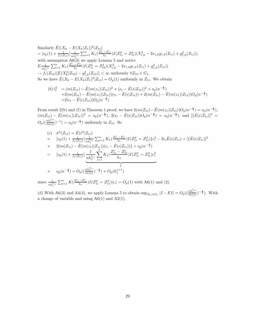
Similarly E((Xk −E(Xk|Z1))2|Z1t)

= [op(1) + 1f1(Z1t)

] 1

nhl1c1

∑ni=1K1(

Zc1i−Zc

1t

h1)I(Zd

1i = Zd1t)(X

2i,k − 2xi,kg1,k(Z1i) + g2

1,k(Z1i)),

with assumption A6(3) we apply Lemma 5 and notice

E 1

nhl1c1

∑ni=1K1(

Zc1i−Zc

10

h1)I(Zd

1i = Zd10)(X

2i,k − 2xi,kg1,k(Z1i) + g2

1,k(Z1i))

→ f1(Z10)[E(X2k |Z10) − g2

1,k(Z10)] <∞ uniformly ∀Z10 ∈ G1.

So we have E(Xk −E(Xk|Z1)2|Z1t) = Op(1) uniformly in Z1t. We obtain

(b) ε2t = (m(Z1t) − E(m(z1)|Z1t))2 + (εt − E(ε|Z1t))

2 + op(n− 1

2 )

+2(m(Z1t) − E(m(z1)|Z1t))(εt − E(ε|Z1t)) + 2(m(Z1t) − E(m(z1)|Z1t))Op(n− 1

2 )

+2(εt − E(ε|Z1t))Op(n− 1

2 )

From result 2(b) and (f) in Theorem 1 proof, we have 2(m(Z1t)−E(m(z1)|Z1t))Op(n− 1

2 ) = op(n− 1

2 ),

(m(Z1t) − E(m(z1)|Z1t))2 = op(n

− 12 ), 2(εt − E(ε|Z1t))Op(n

− 12 ) = op(n

− 12 ), and [E(ε|Z1i)]

2 =

Op((nh

l1c1

ln(n) )−1) = op(n

− 12 ) uniformly in Z1t. So

(c) σ2(Z1t) = E(ε2|Z1t)

= [op(1) + 1f1(Z1t)

] 1

nhl1c1

∑ni=1K1(

Zc1i−Zc

1t

h1)I(Zd

1i = Zd1t)ε2i − 2εiE(ε|Z1i) + [E(ε|Z1i)]

2

+ 2(m(Z1i) − E(m(z1)|Z1i))(εi − E(ε|Z1i)) + op(n− 1

2 )

= [op(1) + 1f1(Z1t)

]1

nhl1c

1

n∑

i=1

K1(Zc

1i − Zc1t

h1)I(Zd

1i = Zd1t)ε

2i

︸ ︷︷ ︸

I

+ op(n− 1

2 ) +Op((nh

l1c1

ln(n) )− 1

2 ) + Op(hs+11 )

since 1

nhl1c1

∑ni=1K(

Zc1i−Zc

1t

h1)I(Zd

1i = Zd1t)|εi| = Op(1) with A6(1) and (2).

(d) With A6(3) and A4(4), we apply Lemma 5 to obtain supZ1t∈G1|I −EI| = Op((

nhl1c1

ln(n) )− 1

2 ). With

a change of variable and using A6(1) and A2(1),

29

EI =∫K1(Ψ)σ2(Zc

1t + h1ψ, Zd1t)f1(Z

c1t + h1ψ, Z

d1t)dψ

=∫K1(Ψ)[σ2(Z1t) +

∑s|j|=1

∂j

∂(Zc1t

)j σ2(Z1t)

h|j|1 Ψj

j!

+∑

|j|=s(∂j

∂(Zc1t

)j σ2(Zc

1t∗, Zd1t) − ∂j

∂(Zc1t

)j σ2(Z1t))

h|j|1 Ψj

j! ][f1(Z1t) +∑s

|l|=1∂l

∂(Zc1t

)l f1(Z1t)h|l|1 Ψl

l!

+∑

|l|=s(∂l

∂(Zc1t

)l f1(Zc1t∗, Zd

1t) − ∂l

∂(Zc1t

)l f1(Z1t))h|l|

1 Ψl

l!]dΨ

= σ2(Z1t)f1(Z1t) + σ2(Z1t)∑s

|j|=1∂j

∂(Zc1t

)j σ2(Z1t)

h|j|1

j!

∫K(1Ψ)ΨjdΨ

+ σ2(Z1t)∑

|j|=s

∫K1(Ψ)( ∂l

∂(Zc1t

)l f1(Zc1t∗, Zd

1t) − ∂l

∂(Zc1t

)l f1(Z1t))h|l|1 Ψl

l! dΨ

+∑s

|j|=1∂j

∂(Zc1t

)j σ2(Z1t)

h|j|1

j!f1(Z1t)

∫K1(Ψ)ΨjdΨ

+∑s

|j|=1∂j

∂(Zc1t

)j σ2(Z1t)

h|j|1

j!(∑s

|l|=1∂l

∂(Zc1t

)l f1(Z1t)h|l|1

l!

∫K1(Ψ)Ψj+ldΨ)

+∑s

|j|=1∂j

∂(Zc1t

)j σ2(Z1t)

h|j|1

j! (∑

|l|=sh|l|1

l!

∫K1(Ψ)( ∂l

∂(Zc1t

)l f1(Zc1t∗, Zd

1t) − ∂l

∂(Zc1t

)l f1(Z1t))Ψj+ldΨ)

+ f1(Z1t)∑

|j|=sh|j|1

j!

∫K1(Ψ)( ∂j

∂(Zc1t

)j σ2(Zc

1t∗, Zd1t) − ∂j

∂(Zc1t

)j σ2(Z1t))Ψ

jdΨ

+∑

|j|=s

∑s|l|=1

∂l

∂(Zc1t

)l f1(Z1t)h|l|1

l!

h|j|1

j!

∫K1(Ψ)( ∂j

∂(Zc1t

)j σ2(Zc

1t∗, Zd1t) − ∂j

∂(Zc1t

)j σ2(Z1t))Ψ

j+ldΨ

+∑

|j|=s

∑

|l|=sh|l|1

l!

h|j|1

j!

∫K1(Ψ)( ∂l

∂(Zc1t

)l f1(Zc1t∗, Zd

1t) − ∂l

∂(Zc1t

)l f1(Z1t))

× ( ∂j

∂(Zc1t

)j σ2(Zc

1t∗, Zd1t) − ∂j

∂(Zc1t

)j σ2(Z1t))Ψ

j+ldΨ

= σ2(Z1t)f1(Z1t) +O(hs+11 ), with the additional assumption A6(1).

The claim in (2) follows from (a)-(d).

(3)√n(βE − βFE)

=√n[(W ′Ω−1(~Z1)W )−1 − (W ′Ω−1(~Z1)W )−1]W ′Ω−1(~Z1)(E(Y | ~Z) − E(Y | ~Z1))

+ (W ′Ω−1(~Z1)W )−1W ′[Ω−1(~Z1) − Ω−1(~Z1)](E(Y | ~Z) − E(Y | ~Z1))So we show

(a) ( 1nW

′Ω−1(~Z1)W )−1 − ( 1nW

′Ω−1(~Z1)W )−1 = op(1).

(b)√n 1

nW′[Ω−1(~Z1) − Ω−1(~Z1)](E(Y | ~Z) − E(Y | ~Z1)) = op(1).

Since in (1) we have√n 1

nW′Ω−1(~Z1)(E(Y | ~Z)−E(Y | ~Z1)) = Op(1), and with (a) ( 1

nW′Ω−1(~Z1)W )−1 p→

(E 1σ2(Z1t)

W ′tWt)

−1, E 1σ2(Z1t)

W ′tWt is positive definite, the claim of (3) follows from (a) and (b).

We first note supZ1t∈G1| 1σ2(Z1t)

− 1σ2(Z1t)

|≤ [infZ1t∈G1 σ

2(Z1t) infZ1t∈G1 σ2(Z1t)]

−1 supZ1t∈G1|σ2(Z1t) − σ2(Z1t)|.

With result (1) and A6(1), for large n, infZ1t∈G1 σ2(Z1t) > 0, so

supZ1t∈G1

| 1

σ2(Z1t)− 1

σ2(Z1t)| = Op((

nhl1c

1

ln(n))−

12 ) + Op(h

s+11 ) + op(n

− 12 ).

(a) Since 1nW ′Ω−1(~Z1)W

p→ E 1σ2(Z1t)

W ′tWt, which is positive definite, so by Slutsky’s Theorem,

( 1nW ′Ω−1(~Z1)W )−1 p→ (E 1

σ2(Z1t)W ′

tWt)−1.

If (a′) 1nW

′(Ω−1(~Z1) − Ω−1(~Z1))W = op(1), then 1nW

′Ω−1(~Z1)Wp→ E 1

σ2(Z1t)W ′

tWt as well, and

( 1nW

′Ω−1(~Z1)W )−1 p→ (E 1σ2(Z1t)

W ′tWt)

−1 so we have the claim in (a). So we only need to show

(a′).

30

The (i, j)th element in 1nW

′(Ω−1(~Z1) − Ω−1(~Z1))W is

1n

∑nt=1 Wt,i(

1σ2(Z1t)

− 1σ2(Z1t)

)Wt,j

= 1n

∑

t[1

σ2(Z1t)− 1

σ2(Z1t)][gi(Zt) − gi(Zt)][gj(Zt) − gj(Zt)]

= 1n

∑

t[1

σ2(Z1t)− 1

σ2(Z1t)][gi(Zt) − gi(Zt)][g1,j(Z1t) − g1,j(Z1t)]

= 1n

∑

t[1

σ2(Z1t)− 1

σ2(Z1t)][gi(Zt) − gi(Zt)][gj(Zt) − g1,j(Z1t)]

= 1n

∑

t[1

σ2(Z1t)− 1

σ2(Z1t)][g1,i(Z1t) − g1,i(Z1t)][gj(Zt) − gj(Zt)]

= 1n

∑

t[1

σ2(Z1t)− 1

σ2(Z1t)][g1,i(Z1t) − g1,i(Z1t)][g1,j(Z1t) − g1,j(Z1t)]

= 1n

∑

t[1

σ2(Z1t)− 1

σ2(Z1t)][g1,i(Z1t) − g1,i(Z1t)][gj(Zt) − g1,j(Z1t)]

= 1n

∑

t[1

σ2(Z1t)− 1

σ2(Z1t)][gi(Zt) − g1,i(Z1t)][gj(Zt) − gj(Zt)]

= 1n

∑

t[1

σ2(Z1t)− 1

σ2(Z1t)][gi(Zt) − g1,i(Z1t)][g1,j(Z1t) − g1,j(Z1t)]

= 1n

∑

t[1

σ2(Z1t)− 1

σ2(Z1t)][gi(Zt) − g1,i(Z1t)][gj(Zt) − g1,j(Z1t)]

= A1 + · · ·+ A9

Since supZ1t∈G1| 1σ2(Z1t)

− 1σ2(Z1t)

| = op(1), we follow Theorem 1 (1) to have Ai = op(1) for

i = 1, · · · , 9. So we have the claim in (a′) and (a).

(b) The kth element in 1nW ′[Ω−1(~Z1) − Ω−1(~Z1)](E(Y | ~Z) − E(Y | ~Z1)) is

Ck = 1n

∑

t[1

σ2(Z1t)− 1

σ2(Z1t)][gk(Zt) − gk(Zt)][E(m(z1)|Zt) − E(m(z1)|Z1t)]

= 1n

∑

t[1

σ2(Z1t)− 1

σ2(Z1t)][g1,k(Z1t) − g1,k(Z1t)][E(m(z1)|Zt) − E(m(z1)|Z1t)]

= 1n

∑

t[1

σ2(Z1t)− 1

σ2(Z1t)][gk(Zt) − g1,k(Z1t)][E(m(z1)|Zt) − E(m(z1)|Z1t)]

= 1n

∑

t[1

σ2(Z1t)− 1

σ2(Z1t)][gk(Zt) − gk(Zt)][E(ε|Zt) − E(ε|Z1t)]

= 1n

∑

t[1

σ2(Z1t)− 1

σ2(Z1t)][g1,k(Z1t) − g1,k(Z1t)][E(ε|Zt) − E(ε|Z1t)]

= 1n

∑

t[1

σ2(Z1t)− 1

σ2(Z1t)][gk(Zt) − g1,k(Z1t)][E(ε|Zt) − E(ε|Z1t)]

With supZ1t∈G1| 1σ2(Z1t)

− 1σ2(Z1t)

| = Op((nh

l1c1

ln(n) )− 1

2 ) + Op(hs+11 ) + op(n

− 12 ), and Theorem 1 proof

(1)(d), (f), (2)(b),(f), we easily have√nCk = op(1), thus we obtain the claim in (b).

31

Appendix 2

Table 1 Bias(×0.1)(B), Standard deviation(S) and Root MeanSquared Error(R) for estimators with g1 and σ2

1

n = 100 θ = 0.2 θ = 0.5 θ = 0.8estimators B S R B S R B S R

β1 .963 .073 .121 2.469 .066 .256 3.947 .052 .398

β2 .050 .119 .119 .062 .124 .124 -.104 .127 .128

β -.022 .107 .107 -.011 .110 .110 -.109 .113 .113

β .879 .107 .139 1.360 .108 .174 1.789 .104 .207

β .262 .095 .099 .663 .094 .115 .991 .088 .133

βE .266 .101 .105 .685 .100 .121 1.030 .093 .139

n = 200 θ = 0.2 θ = 0.5 θ = 0.8estimators B S R B S R B S R

β1 .988 .050 .111 2.461 .047 .251 3.959 .035 .397

β2 .051 .079 .079 -.007 .082 .082 -.021 .079 .079

β -.031 .073 .073 -.060 .074 .074 -.076 .071 .072

β .768 .073 .106 1.117 .075 .134 1.448 .069 .161

β .159 .068 .070 .404 .067 .079 .627 .062 .088

βE .160 .070 .072 .413 .069 .081 .644 .064 .091

Table 2 Bias(B), Standard deviation(S) and Root MeanSquared Error(R) for estimators with g2 and σ2

1

n = 100 θ = 0.2 θ = 0.5 θ = 0.8estimators B S R B S R B S R

β1 .152 .091 .177 .384 .079 .392 .630 .058 .632

β2 .525 10.177 10.185 .294 9.011 9.011 .285 24.627 24.617

β .182 3.589 3.592 .178 12.492 12.487 .532 1.906 1.978

β .215 .209 .300 .353 .205 .409 .504 .215 .548

β .093 .152 .178 .204 .141 .248 .333 .118 .353

βE .099 .160 .188 .214 .150 .261 .342 .126 .364

n = 200 θ = 0.2 θ = 0.5 θ = 0.8estimators B S R B S R B S R

β1 .155 .066 .168 .390 .051 .393 .627 .039 .628

β2 .629 20.838 20.838 3.628 57.572 57.657 4.768 157.262 157.255

β .183 3.215 3.218 .393 3.078 3.101 .599 2.416 2.488

β .221 .151 .268 .325 .146 .356 .436 .150 .461

β .073 .118 .138 .156 .108 .189 .237 .092 .255

βE .076 .121 .143 .160 .111 .194 .241 .093 .259

32

Table 3 Bias(×0.1)(B), Standard deviation(S) and Root MeanSquared Error(R) for estimators with g1 and σ2

2

n = 100 θ = 0.2 θ = 0.5 θ = 0.8

estimators B S R B S R B S R

β1 .345 .058 .067 1.028 .054 .116 1.674 .052 .175

β2 .033 .054 .054 .049 .054 .054 -.005 .057 .057

β -.124 .060 .062 -.096 .059 .060 -.120 .062 .063

β .376 .062 .073 .594 .062 .086 .741 .064 .098

β .038 .058 .058 .221 .056 .060 .346 .056 .066

βE .012 .038 .038 .076 .037 .038 .106 .038 .040

n = 200 θ = 0.2 θ = 0.5 θ = 0.8

estimators B S R B S R B S R

β1 .385 .039 .055 1.051 .037 .111 1.719 .035 .175

β2 .045 .035 .035 .022 .037 .037 .030 .036 .036

β -.071 .039 .039 -.095 .042 .043 -.086 .041 .042

β .406 .041 .058 .509 .044 .067 .655 .043 .078

β .033 .039 .039 .105 .041 .042 .209 .039 .044

βE .003 .024 .024 .017 .024 .024 .033 .024 .024

Table 4 Bias(B), Standard deviation(S) and Root MeanSquared Error(R) for estimators with g2 and σ2

2

n = 100 θ = 0.2 θ = 0.5 θ = 0.8

estimators B S R B S R B S R

β1 .097 .093 .134 .242 .084 .256 .397 .069 .403

β2 .208 10.796 10.792 .353 8.366 8.370 .844 13.184 13.204β .076 2.955 2.954 .227 2.620 2.629 .197 2.703 2.709

β .115 .143 .183 .177 .141 .226 .242 .141 .280

β .063 .107 .125 .112 .100 .151 .170 .092 .194

βE .016 .075 .076 .037 .079 .087 .063 .082 .104

n = 200 θ = 0.2 θ = 0.5 θ = 0.8

estimators B S R B S R B S R

β1 .093 .065 .113 .251 .055 .257 .407 .043 .409

β2 -.036 24.853 24.840 .199 16.715 16.708 .302 6.619 6.623

β .131 2.197 2.200 .155 2.211 2.215 .341 1.546 1.582

β .118 .095 .151 .172 .094 .196 .219 .093 .238

β .042 .071 .083 .085 .071 .111 .123 .066 .140

βE .075 .044 .045 .015 .045 .047 .030 .044 .053

33

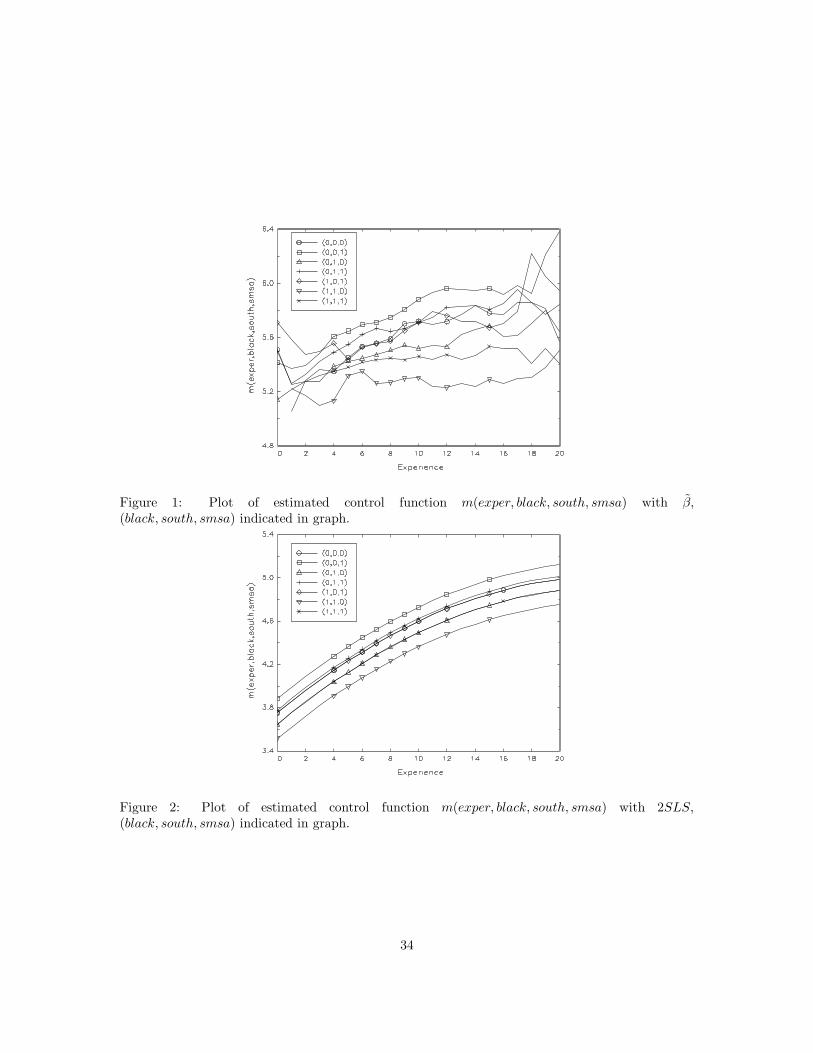
Figure 1: Plot of estimated control function m(exper, black, south, smsa) with β,(black, south, smsa) indicated in graph.

Figure 2: Plot of estimated control function m(exper, black, south, smsa) with 2SLS,(black, south, smsa) indicated in graph.

34

Figure 3: Plot of estimated log(wage) using β and 2SLS against realized log(wage).

35

References

[1] Ai, C. and X. Chen, 2003, Efficient estimation of models with conditional moment restrictionscontaining unknown functions. Econometrica, 71, 1975-1843.

[2] Aneiros, G. and A. Quintela, 2001, Asymptotic properties in partial linear models under depen-dence. Test, 10, 333-355.

[3] Aneiros-Perez, G. and A. Quintela-del-Rio, 2002, Plug-in bandwidth choice in partial linearmodels with autoregressive errors. Journal of Statistical Planning and Inference, 100, 2348.

[4] Baltagi, B. H. and Q. Li, 2002, On instrumental variable estimation of semiparametric dynamicpanel data models. Economics letters, 76, 1-9.

[5] Basmann, R. L., A generalized classical method of linear estimation of coefficients in a structuralequation. Econometrica, 25, 77-83.

[6] Bickel, P., 1982, On adaptive estimation. Annals of statistics, 10, 647-671.

[7] Berg, M. D., Q. Li, and A. Ullah, 2000, Instrumental variable estimation of semiparametricdynamic panel data models: Monte Carlo results on several new and existing estimators. Nonsta-tionary panels, panel cointegration and dynamic panels, 15, 297-315, Elsevier science Inc..

[8] Blundell,R., and Powell, J.L., 2001, Endogeneity in nonparametric and semiparametric regres-sion models. Centre for Microdata Methods and Practice, Institute for Fiscal Studies, CeMMAPworking papers with number CWP09/01.

[9] Camlong-Viot, C., Rodrguez-Poo,J.M., and Vieu, P., 2006, Nonparametric and semiparametricestimation of additive models with both discrete and continuous variables under dependence. Theart of semiparametrics, 155-178, Physica-Verlag HD.

[10] Card, D., 1995, Using geographic variation in college proximity to estimate the return to school-ing, in Aspects of labour market behavior: essays in honour of John Vanderkamp. Ed. L. N.Christophides, E. K. Grant and R. Swidinsky, 201-222. Toronto: University of Toronto Press.

[11] Chamberlain, G., 1992, Efficiency bounds for semiparametric regression. Econometrica, 60,567-596.

[12] Chen, S., 1999, Distribution-free estimation of the random coefficient dummy endogenous vari-able model. Journal of Econometrics, v 91, 171-199.

[13] Das, M., 2005, Instrumental variable estimation of models with discrete endogenous regressors.Journal of Econometrics, v 124, 335-361.

[14] Darolles, S., J.-P. Florens, and E. Renault, 2003, Nonparametric Instrumental Regression.Working Paper, Toulouse University.

[15] Davidson, R., and J. G. MacKinnon, 2004, Econometric theory and methods. Oxford universitypress, New York.

[16] Delgado, M.A., and J. Mora, 1995, Nonparametric and semiparametric estimation with discreteregressors. Econometrica, 63, 1477-1484.

36

[17] Fan, J., Hardle, W. and Mammen, E.,1998, Direct estimation of low dimensional componentsin additive models. The Annals of Statistics, 26, 943-971.

[18] Florens, J. P., J. J. Heckman, C. Meghir, and E. Vytlacil, 2008, Identification of treatmenteffects using control functions in models with continuous, endogenous treatment and heterogeneouseffects. Econometrica, 76, 11911206.

[19] Hardle, W., Liang, H. and J. Gao (2000), Partially linear models. Physica-Verlag.

[20] Heckman, J. J., 1978, Dummy endogenous variables in a simultaneous equation system. Econo-metrica, 46, 931-959.

[21] Heckman, J. J. and R. Robb, 1985, Alternative methods for evaluating the impact of inter-ventions, in Longitudinal analysis of labor market data, ed. by J. J. Heckman and B. Singer.Cambridge, England: Cambridge University Press.

[22] Imbens and Newey, 2009, Identification and estimation of triangular simultaneous equationsmodels without additivity, forthcoming in Econometrica.

[23] Li, Q., and Stengos, T., 1996, Semiparametric estimation of partially linear panel data models.Journal of Econometrics, 71, 389-397.

[24] Li, Q. and A. Ullah, 1998, Estimating partially linearl panel data models with one-way errorcomponents. Econometric reviews, 17, 145-166.

[25] Martins-Filho, C. and F. Yao, 2007,Nonparametric frontier estimation via local linear regression.Journal of Econometrics, 141/1, 283-319.

[26] Matzkin, R.L.,1994, Restrictions of economic theory in nonparametric methods. In Handbook ofEconometrics: vIV, edited by R. F. Engle, and D. L. McFadden, Elsevier Science, North Holland.

[27] Matzkin, R.L.,2008, Identification in nonparametric simultaneous equations, forthcoming inEconometrica.

[28] Manski, C. F., 1984, Adaptive estimation of nonlinear regression models. Econometric reviews,3, 145-194.

[29] Newey, W. K., 1990, Efficient instrumental variable estimation of nonlinear models. Economet-rica, 58, 809-837.

[30] Newey, W. K., 1993, Efficient estimation of models with conditional moment restrictions. InHandbook of Statistics, v 11, 419-454, G.S. Maddala, C.R. Rao, and H.D. Vinod, eds., Amsterdam:North-Holland.

[31] Newey, W.K. and J.L. Powell, 1989, Nonparametric Instrumental Variables Estimation, MITworking paper.

[32] Newey, W. K., J. L. Powell, and F. Vella, 1999, Nonparametric estimation of triangular simul-taneous equations models. Econometrica, 67, 565603.

[33] Newey, W. K., J. L. Powell and J. R. Walker, 1990, Semiparametric estimation of selectionmodels: some empirical results. The american economic review, 80, No. 2, papers and proceedingsof the hundred and second annual meeting of the american economic association, 324-328.

37

[34] Ng, S. and J. Pinkse, 1995, Nonparametric two step estimation of unknown regression func-tion when the regressors and the regressor error are not independent. Manuscript, University ofMontreal.

[35] Pinkse, J., 2000, Nonparametric two-step regression functions when regressors and error aredependent. Canadian Journal of Statistics, 28, 289300.

[36] Powell, J. L., J. H. Stock and T. M. Stoker, 1989, Semiparametric estimation of the indexcoefficients. Econometrica, 57, 1403-1430.

[37] Racine, J. and Li, Q., 2000, Nonparametric estimation of regression functions with both cate-gorical and continuous data. Journal of Econometrics, 119, 99-130.

[38] Rilstone, P., 1992, Semiparametric IV estimation with parameter dependent instruments.Econometric Theory, 8, 403-406.

[39] Robinson, P., 1987, Root-n-consistent semiparametric regression. Econometrica, 56, 931-954.

[40] Speckman, P., 1988, Kernel smoothing in partial linear models. Journal of the Royal StatisticalSociety, Series B, 50, 413-436.

[41] Ruppert, D., S. J. Sheather, M. P. Wand, 1995, An effective bandwidth selector for local leastsquares regression. Journal of the American Statistical Association, 90, 1257-1270.

[42] Theil, H., 1953, Repeated least squares applied to complete equation systems. The Hague:central planning bureau.

[43] White, H., 1980, A heteroskedasticity-consistent covariance matrix estimator and a direct testfor heteroskedasticity. Econometrica, 48, 817-38.

38