January 03 LASERS 51

Imaging with two lenses• Graphical methods

– Parallel-ray method, find intermediate image, use as object for next lens

– Virtual objects– Oblique-ray method, lens-to-lens, no need to find

intermediate image

• Mathematical methods– Find intermediate image, use as object for next lens– lens-to-lens (sequential raytracing)-later in semester

• Combinations of thin lenses– In contact– Separated

January 03 LASERS 51

Example, two separated positive lenses

• Needed information– focal lengths of lenses– location of lenses– location of object

L1 L2

F1F1'

F2

F2'Object

January 03 LASERS 51

Parallel-ray method - step 1

• Ignore second lens• Trace at least two of the rays shown from tip of object

– tip of image found from intersection of rays– exactly as we did in previous module– NOTE: all rays from tip of object intersect at tip of image we

have chosen three only because they are easy to trace!– Image is real in this case, but method is exactly the same if it

is virtual WHENEVER NEEDED YOU MAY EXTEND OBJECT-SPACE OR IMAGE-SPACE RAYS TO INFINITY IN EITHER DIRECTION

L1

F1F1'

Object

Image

January 03 LASERS 51

Parallel-ray method - step 2

• Image from step 1 becomes Object for step 2– After producing this object, lens1 one can be ignored– object can be real or virtual (virtual in this case)– object can be real even if image from lens 1 is virtual

• Trace any two of the three rays shown through tip of object to find tip of final image– Final image may be real or virtual (real in this case)

L2

F2

F2'

Object(virtual)

Image(real)

January 03 LASERS 51

Reminder about real and virtual objects and images

• Positive distances correspond to real objects and real images– Object distance positive when it is to the left of the lens– Image distance positive when it is to the right of the lens– This is the common situation for a single positive image

forming an image on a screen, Examples- viewgraph machine, camera, eye, etc.

• Negative distances correspond to virtual objects and virtual images– Object to the right or image to the left of the lens

Remember: For purposes of calculations, light travels from left to right (not necessarily in real life, of course)

January 03 LASERS 51

Oblique-ray method• Is it really necessary to find the image due to the first lens?• Any ray can be traced through the lens system using the

oblique-ray method• For example, trace the axial ray

– point of intersection with axis in image space gives image location

L1 L2

F1F1'

F2

F2'Object

parallel

axial ray

Image

parallel

secondfocal planeof lens1

secondfocal planeof lens2

January 03 LASERS 51

Imaging through multiple lenses -mathematical

• Apply imaging formula to first lens to find image in that lens

• Find object distance for second lens (negative means virtual object)

• Use imaging formula again to find final image

L1 L2

F1F1'

F2

F2'Object

s1 s1'-s2d

s2'

Fina

l Im

age

Inte

rmed

iate

Imag

e

11

111 fs

fss−

=′

12 sds ′−=

22

222 fs

fss−

=′

Given, f1, f2, d, and s1 find s2’

January 03 LASERS 51

Magnification with multiple lenses• The magnification is by definition the image size

divided by the object size• For the second lens in a system the object size is

the image size for the first lens

1112 yMyy =′=• The image size after the second lens is found by

multiplying the second lens magnification by the size of the object for the second lens

121222 yMMyMy ==′• The system magnification is the final image size

divided by the original object size

21MMMsystem =

January 03 LASERS 51

Symbols for thin lenses

• Arrows symbolize the outline of the glass at the edge

January 03 LASERS 51

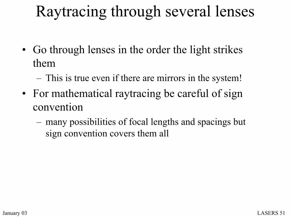
Raytracing through several lenses

• Go through lenses in the order the light strikes them– This is true even if there are mirrors in the system!

• For mathematical raytracing be careful of sign convention– many possibilities of focal lengths and spacings but

sign convention covers them all

January 03 LASERS 51

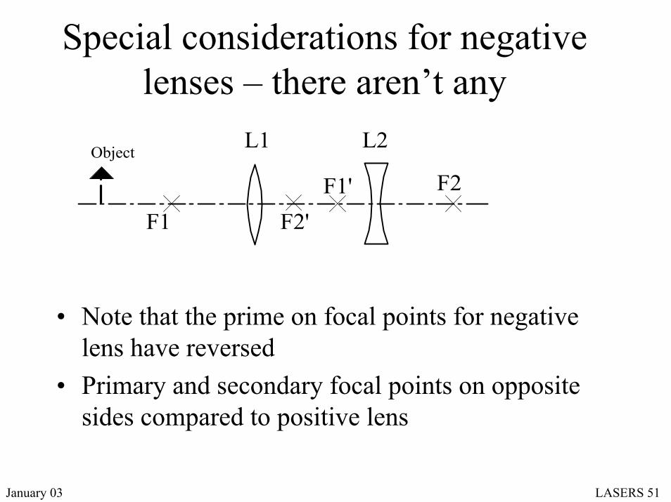
Special considerations for negative lenses – there aren’t any

L1 L2

F1F1'

F2'

F2Object

• Note that the prime on focal points for negative lens have reversed

• Primary and secondary focal points on opposite sides compared to positive lens

January 03 LASERS 51

Principal planes and focal lengths of multi-lens systems

secondprincipalplane

secondfocalpoint

• Defined exactly the same as for thick lens

January 03 LASERS 51

Thin lenses in contact

21

111fff

+= 21 PPP +=

• Can be applied to multiple thin lenses in contact as well

• As always, be careful with sign convention

January 03 LASERS 51

Dispersion-Abbe V number

• Index of refraction changes with wavelength

• Usually decreases for longer wavelengths• Small, but important effect

Index of refraction of Quartz

1.454

1.456

1.458

1.460

1.462

1.464

1.466

1.468

1.470

1.472

350 400 450 500 550 600 650 700

Wavelength (nm)

Refra

ctiv

e In

dex

CdF

nC=1.45646nd=1.45857

nF=1.46324

Blue Green RedGlass designationQuartz, 459676BK7, 517642

Abbe V number-Definition

CF

dd nn

nV−−

=1

For Quartz, Vd=67.6

January 03 LASERS 51

Glass map - index/dispersion of glasses

January 03 LASERS 51

Chromatic aberration of thin lenses

f_Cf_d

f_F

−−=

21

11)1(RR

nP FF

−−=

21

11)1(RR

nP CC

( )d

d

d

dCFcFCF V

Pn

PnnRR

nnPP =−

−=

−−=−

111)(

21

• Called longitudinal chromatic aberration– This is the only chromatic aberration possible in a

single thin lens with the stop at the lens

January 03 LASERS 51

Achromatic doubletsPositivehigh indexlow dispersion

Negativelow index

high dispersion

ddd PPP −+ +=

To achieve the desired focal length requires

Many choices of powers satisfy this

( ) ( )d

d

d

dCFCFCF V

PVPPPPPPP

−

−

+

+−−++ +=−+−==− 0

We can also choose the powers to make chromatic zero

• Two radii used to get each power, one can be freely chosen• One is usually chosen to make inner surfaces have the

same curvature (cemented doublet)• Remaining radius chosen to minimize spherical aberration

January 03 LASERS 51

Thin lenses separated• Two positive thin

lenses are weaker in combination when separated than when in contact

• Use of these equation in solving homework problems is discouraged

d

F

FB

2121

111ffd

fff−+= 2121 PdPPPP −+=

Ffd

PfdFB

−=

−=

11

111

Back focal length

dPPFFB 1−=−

Second lens to principal plane

January 03 LASERS 51

Principal plane locations for thin lens combinations

• c1 is power of first lens• f2 is focal length of second

lens• Focal length of

combination is kept constant at 100 mm

Second principal plane

First principal plane