image classi cation: a study in age-related macular

Image Classification: A Study in Age-related

Macular Degeneration Screening

Thesis submitted in accordance with the requirements ofthe University of Liverpool for the degree of Doctor in Philosophy

byMohd Hanafi Ahmad Hijazi

July 2012

To my family, especially to my wife, Mariati, and mychildren, Aidil and Dina.

Abstract

This thesis presents research work conducted in the field of image mining. More specif-

ically, the work is directed at the employment of image classification techniques to

classify images where features of interest are very difficult to distinguish. In this con-

text, three distinct approaches to image classification are proposed. The first is founded

on a time series based image representation, whereby each image is defined in terms of

histograms that in turn are presented as “time series” curves. A Case Based Reason-

ing (CBR) mechanism, coupled with a Time Series Analysis (TSA) technique, is then

applied to classify new “unseen” images. The second proposed approach uses statisti-

cal parameters that are extracted from the images either directly or indirectly. These

parameters are then represented in a tabular form from which a classifier can be built

on. The third is founded on a tree based representation, whereby a hierarchical decom-

position technique is proposed. The images are successively decomposed into smaller

segments until each segment describes a uniform set of features. The resulting tree

structures allow for the application of weighted frequent sub-graph mining to identify

feature vectors representing each image. A standard classifier generator is then applied

to this feature vector representation to produce the desired classifier. The presented

evaluation, applied to all three approaches, is directed at the classification of retinal

colour fundus images; the aim is to screen for an eye condition known as Age-related

Macular Degeneration (AMD). Of all the approaches considered in this thesis, the tree

based representation coupled with weighted frequent sub-graph mining produced the

best performance. The evaluation also indicated that a sound foundation has been

established for future potential AMD screening programmes.

ii

Acknowledgement

First and Foremost, praise be to God, the Most Gracious and Most Merciful, for giv-

ing me the strength, and the wonderful people that surround me, that have kept me

standing and believing that my efforts would bear fruit.

Of all the fantastic and fabulous people involved, I am fully indebted (and would

like to express my deepest gratitude) to my first supervisor Dr. Frans Coenen who has

been abundantly helpful and has offered invaluable assistance, support and guidance

throughout my Ph.D. study and which has made it one of the most enjoyable and

unforgettable experience ever. It is my privileged to have worked with him. Deepest

gratitude is also due to my second supervisor Dr. Yalin Zheng without whose knowledge

and assistance this research would not have been successful. I will surely miss our once

a month coffee session at the hospital!

Special thanks also go to my former Ph.D. colleagues, Chuntao Jiang (Geof) for

our collaborative research work, and Ashraf Elsayed for giving me some ideas during

the first year of my research. Special thanks also to all the staff in the Department

of Computer Science at The University of Liverpool and the St. Paul’s Eye Unit at

the Royal Liverpool University Hospital that have been helpful whenever needed. Not

forgetting my fellow colleagues in Room 2.11 who always encouraged each other either

directly or indirectly; my prayers go to all of you to succeed in everything that you do.

I would also like to convey thanks to the Malaysian Government, more specifically

to the Ministry of Higher Education and Universiti Malaysia Sabah, for providing me

with the opportunity and financial means to conduct my Ph.D. study.

Last, but not least, love and gratitude to my beloved family; especially to my parent,

my wife and my two wonderful children, for their understanding and constant support,

without whom the completion of my Ph.D. would have not been possible.

iii

Contents

Abstract ii

Acknowledgement iii

Contents iii

List of Figures ix

List of Tables xii

Abbreviations xv

1 Introduction 1

1.1 Overview . . . . . . . . . . . . . . . . . . . . . . . . . . . . . . . . . . . 1

1.2 Motivation . . . . . . . . . . . . . . . . . . . . . . . . . . . . . . . . . . 2

1.3 Research Objectives . . . . . . . . . . . . . . . . . . . . . . . . . . . . . 4

1.4 Research Contributions . . . . . . . . . . . . . . . . . . . . . . . . . . . 5

1.5 Research Methodology . . . . . . . . . . . . . . . . . . . . . . . . . . . . 6

1.6 Criteria for Success . . . . . . . . . . . . . . . . . . . . . . . . . . . . . . 7

1.7 Published Work . . . . . . . . . . . . . . . . . . . . . . . . . . . . . . . . 11

1.8 Structure of Thesis . . . . . . . . . . . . . . . . . . . . . . . . . . . . . . 14

2 Image Datasets 15

2.1 Introduction . . . . . . . . . . . . . . . . . . . . . . . . . . . . . . . . . . 15

2.2 The Human Eye Anatomy . . . . . . . . . . . . . . . . . . . . . . . . . . 15

2.3 Age-related Macular Degeneration . . . . . . . . . . . . . . . . . . . . . 17

2.4 Retinal Image Datasets . . . . . . . . . . . . . . . . . . . . . . . . . . . 18

2.4.1 ARIA Dataset . . . . . . . . . . . . . . . . . . . . . . . . . . . . 19

2.4.2 STARE Dataset . . . . . . . . . . . . . . . . . . . . . . . . . . . 20

2.5 Summary . . . . . . . . . . . . . . . . . . . . . . . . . . . . . . . . . . . 20

3 Literature Review and Previous Work 21

3.1 Introduction . . . . . . . . . . . . . . . . . . . . . . . . . . . . . . . . . . 21

iv

3.2 Digital Image Representation . . . . . . . . . . . . . . . . . . . . . . . . 22

3.2.1 Image Quality . . . . . . . . . . . . . . . . . . . . . . . . . . . . 24

3.2.2 Image Storage Formats . . . . . . . . . . . . . . . . . . . . . . . 24

3.2.3 Colour Models . . . . . . . . . . . . . . . . . . . . . . . . . . . . 25

3.3 Knowledge Discovery in Databases . . . . . . . . . . . . . . . . . . . . . 27

3.3.1 The Knowledge Discovery in Databases Process . . . . . . . . . . 28

3.3.2 Data Mining . . . . . . . . . . . . . . . . . . . . . . . . . . . . . 29

3.3.3 Issues in Knowledge Discovery in Databases . . . . . . . . . . . . 30

3.4 The Image Classification Process . . . . . . . . . . . . . . . . . . . . . . 32

3.4.1 Image Acquisition (Domain Understanding and Data Selection) . 33

3.4.2 Image Pre-processing (Data Pre-processing) . . . . . . . . . . . . 33

3.4.3 Feature Extraction and Selection (Data Transformation) . . . . . 33

3.4.4 Classifier Generation (Data Mining) and Classification . . . . . . 35

3.5 Image Representation for Data Mining . . . . . . . . . . . . . . . . . . . 36

3.5.1 Time Series Image Representation . . . . . . . . . . . . . . . . . 36

3.5.1.1 Colour Histograms as Image Features . . . . . . . . . . 38

3.5.2 Tabular Image Representation . . . . . . . . . . . . . . . . . . . 40

3.5.2.1 Statistical Parameters as Image Features . . . . . . . . 41

3.5.3 Tree Image Representation . . . . . . . . . . . . . . . . . . . . . 43

3.5.3.1 Frequent Sub-trees as Image Features . . . . . . . . . . 47

3.6 Review of Selected Classification Techniques . . . . . . . . . . . . . . . . 49

3.6.1 Bayesian Networks . . . . . . . . . . . . . . . . . . . . . . . . . . 49

3.6.2 Support Vector Machines . . . . . . . . . . . . . . . . . . . . . . 50

3.6.3 k-Nearest Neighbours . . . . . . . . . . . . . . . . . . . . . . . . 52

3.6.4 Image Classification Applications . . . . . . . . . . . . . . . . . . 53

3.7 Case Based Reasoning for Image Classification . . . . . . . . . . . . . . 53

3.7.1 Overview of Case Based Reasoning . . . . . . . . . . . . . . . . . 54

3.7.2 Similarity Measures . . . . . . . . . . . . . . . . . . . . . . . . . 55

3.7.3 Applications of Case Based Reasoning for Image Classification . 55

3.8 Image Classification for the Screening of Age-related Macular Degeneration 56

3.9 Summary . . . . . . . . . . . . . . . . . . . . . . . . . . . . . . . . . . . 57

4 Image Pre-Processing 59

4.1 Introduction . . . . . . . . . . . . . . . . . . . . . . . . . . . . . . . . . . 59

4.2 Image Enhancement . . . . . . . . . . . . . . . . . . . . . . . . . . . . . 60

4.2.1 Region of Interest Identification using Image Mask . . . . . . . . 62

4.2.2 Colour Normalisation . . . . . . . . . . . . . . . . . . . . . . . . 63

4.2.3 Illumination Normalisation . . . . . . . . . . . . . . . . . . . . . 67

4.2.4 Contrast Enhancement . . . . . . . . . . . . . . . . . . . . . . . . 69

4.3 Image “Noise” Removal . . . . . . . . . . . . . . . . . . . . . . . . . . . 71

v

4.4 Summary . . . . . . . . . . . . . . . . . . . . . . . . . . . . . . . . . . . 74

5 Time Series Based Image Representation for Image Classification 76

5.1 Introduction . . . . . . . . . . . . . . . . . . . . . . . . . . . . . . . . . . 76

5.2 Features Extraction . . . . . . . . . . . . . . . . . . . . . . . . . . . . . 79

5.2.1 Colour Histogram Generation . . . . . . . . . . . . . . . . . . . . 79

5.2.2 Colour Histogram Generation without Optic Disc . . . . . . . . . 82

5.2.2.1 The Optic Disc Segmentation and Removal . . . . . . . 82

5.2.3 Spatial-Colour Histogram Generation . . . . . . . . . . . . . . . 87

5.3 Features Selection . . . . . . . . . . . . . . . . . . . . . . . . . . . . . . 88

5.4 Classification Technique . . . . . . . . . . . . . . . . . . . . . . . . . . . 89

5.4.1 Dynamic Time Warping . . . . . . . . . . . . . . . . . . . . . . . 90

5.4.2 Time Series Case Based Reasoning for Image Classification . . . 92

5.4.2.1 Image Classification using a Single Case Base . . . . . . 92

5.4.2.2 Image Classification using Two Case Bases . . . . . . . 94

5.5 Evaluation and Discussion . . . . . . . . . . . . . . . . . . . . . . . . . . 96

5.5.1 Experimental Set Up . . . . . . . . . . . . . . . . . . . . . . . . . 96

5.5.2 Experiment 1: Comparison of Classification Performances using

Different W Values . . . . . . . . . . . . . . . . . . . . . . . . . . 98

5.5.2.1 Discussion of Experiment 1 Results . . . . . . . . . . . 99


Different Numbers of Case Bases . . . . . . . . . . . . . . . . . . 100


5.5.4 Experiment 3: Comparison of Performances using Different Val-

ues of T . . . . . . . . . . . . . . . . . . . . . . . . . . . . . . . . 104


5.5.5 Overall Discussion . . . . . . . . . . . . . . . . . . . . . . . . . . 107

5.6 Summary . . . . . . . . . . . . . . . . . . . . . . . . . . . . . . . . . . . 108

6 Tabular Based Image Representation for Image Classification 110

6.1 Introduction . . . . . . . . . . . . . . . . . . . . . . . . . . . . . . . . . . 111

6.2 Features Extraction . . . . . . . . . . . . . . . . . . . . . . . . . . . . . 111

6.3 Features Selection . . . . . . . . . . . . . . . . . . . . . . . . . . . . . . 116

6.4 Classifier Generation . . . . . . . . . . . . . . . . . . . . . . . . . . . . . 119

6.5 Classification Strategies for Multiclass Classification . . . . . . . . . . . 120




Strategy S1 and S2 . . . . . . . . . . . . . . . . . . . . . . . . . . 123

6.6.2.1 Classification Results using the BD Dataset . . . . . . . 123

vi

6.6.2.2 Classification Results using the MD Dataset . . . . . . . 125


6.6.3 Experiment 2: Comparison of Different Values of T . . . . . . . . 129

6.6.3.1 Classification Results using the BD Dataset . . . . . . . 129

6.6.3.2 Classification Results using the MD Dataset . . . . . . . 134


6.6.4 Overall Discussion . . . . . . . . . . . . . . . . . . . . . . . . . . 139

6.7 Summary . . . . . . . . . . . . . . . . . . . . . . . . . . . . . . . . . . . 139

7 Tree Based Image Representation for Image Classification 141

7.1 Introduction . . . . . . . . . . . . . . . . . . . . . . . . . . . . . . . . . . 141

7.2 Image Decomposition for Tree Generation . . . . . . . . . . . . . . . . . 142

7.2.1 Termination Criterion . . . . . . . . . . . . . . . . . . . . . . . . 147

7.3 Feature Exraction . . . . . . . . . . . . . . . . . . . . . . . . . . . . . . 148

7.3.1 Frequent Sub-graph Mining . . . . . . . . . . . . . . . . . . . . . 148

7.3.2 Weighted Frequent Sub-graph Mining . . . . . . . . . . . . . . . 150

7.4 Feature Selection . . . . . . . . . . . . . . . . . . . . . . . . . . . . . . . 154

7.5 Classification Technique . . . . . . . . . . . . . . . . . . . . . . . . . . . 154




Various Dmax Values . . . . . . . . . . . . . . . . . . . . . . . . . 156


7.6.3 Experiment 2: Comparison of Different Values of K . . . . . . . 161


7.7 Summary . . . . . . . . . . . . . . . . . . . . . . . . . . . . . . . . . . . 167

8 Comparison Between Different Approaches 169

8.1 Comparison of the Proposed Approaches in Terms of AMD Classification 169

8.2 Statistical Comparison of the Proposed Approaches . . . . . . . . . . . . 172

8.3 Summary . . . . . . . . . . . . . . . . . . . . . . . . . . . . . . . . . . . 176

9 Conclusion 179

9.1 Summary . . . . . . . . . . . . . . . . . . . . . . . . . . . . . . . . . . . 179

9.2 Main Findings and Contributions . . . . . . . . . . . . . . . . . . . . . . 180

9.3 Future Work . . . . . . . . . . . . . . . . . . . . . . . . . . . . . . . . . 182

Bibliography 184

Index 201

vii

Appendix 201

A Studentised Range Statistic Table 202

B F Distribution Table 204

viii

List of Figures

1.1 Example of a retinal image . . . . . . . . . . . . . . . . . . . . . . . . . 4

1.2 Confusion matrix . . . . . . . . . . . . . . . . . . . . . . . . . . . . . . . 8

1.3 An example of ROC curves . . . . . . . . . . . . . . . . . . . . . . . . . 10

2.1 The anatomy of human eye [2] . . . . . . . . . . . . . . . . . . . . . . . 16

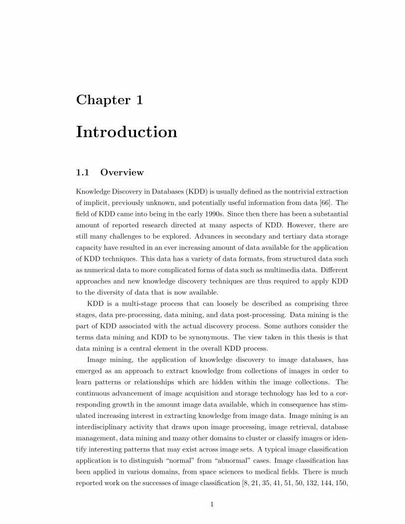
2.2 Example of: (a) normal, (b) early AMD, and (c) advanced neovascular

AMD retinal images . . . . . . . . . . . . . . . . . . . . . . . . . . . . . 18

2.3 Vision of (a) a normal people and (b) an AMD patient (taken from

http://www.nei.nih.gov/health/maculardegen/armdfacts.asp) . . . . . . 19

2.4 Example of retinal images acquired from ARIA (top row) and STARE

(bottom row) datasets . . . . . . . . . . . . . . . . . . . . . . . . . . . . 19

3.1 Example of an 8×8 image with its corresponding 2-D array representa-

tion [175] . . . . . . . . . . . . . . . . . . . . . . . . . . . . . . . . . . . 23

3.2 Example of (a) RGB, (b) grey-scale and (c) binary image data types . . 25

3.3 (a) The RGB model cube and (b) the HSI model [74] . . . . . . . . . . . 27

3.4 KDD process functional steps [56, 130] . . . . . . . . . . . . . . . . . . . 29

3.5 Image classifier generation process [9] . . . . . . . . . . . . . . . . . . . . 32

3.6 An example of grey-scale retinal images represented as time series . . . 37

3.7 Example of images represented in a tabular form . . . . . . . . . . . . . 40

3.8 Example of two different 2-D array represented images that have identi-

cal global colour mean values . . . . . . . . . . . . . . . . . . . . . . . . 41

3.9 Examples of: (a) complete, (b) regular, (c) cycle, and (d) labelled graphs. 45

3.10 Examples of (a) labelled ordered tree, and (b) sub-tree of (a) . . . . . . 45

3.11 An example of images represented in the form of tree data structure . . 46

3.12 Block diagram of CBR cycle . . . . . . . . . . . . . . . . . . . . . . . . . 54

4.1 Illustration of the enhancement of a retinal image: (a) original image, (b)

image mask for image in (a), (c) reference image, (d) image in (a) after

colour normalisation, (e) image in (d) after illumination normalisation

and (f) image in (e) after contrast enhancement . . . . . . . . . . . . . . 61

ix

4.2 Example of the colour normalisation task as adopted in this thesis: (a)

target image pixel intensity values, (b) target image colour histogram

extracted from (a), (c) reference image colour histogram, (d) target im-

age colour histogram after histogram specification, and (e) target image

pixel intensity values after histogram specification . . . . . . . . . . . . 66

4.3 Example of retinal images and their corresponding colour histograms

for colour normalisation: (a) unnormalised retinal image; (b) reference

image; (c) image in (a) after colour normalisation; (d), (e) and (f) the

RGB histograms of the images in (a), (b) and (c) respectively . . . . . . 68

4.4 Example of the illumination normalisation technique applied to a retinal

image: (a) colour normalised retinal image, (b) the identified background

pixels of the image in (a), (c) the green channel luminosity estimate

image, and (d) the image in (a) after illumination normalisation . . . . 70

4.5 Noise removal tasks: (a) green channel of the enhanced colour image, (b)

retinal blood vessels segmented and (c) image mask and retinal blood

vessels pixels removed . . . . . . . . . . . . . . . . . . . . . . . . . . . . 74

5.1 The CB construction process for the proposed time series based image

classification using different forms of feature extraction: (a) colour his-

tograms, (b) colour histograms without optic disc information and (c)

spatial-colour histograms. . . . . . . . . . . . . . . . . . . . . . . . . . . 78

5.2 Example of time series sequences, (a) before normalisation and (b) after

normalisation . . . . . . . . . . . . . . . . . . . . . . . . . . . . . . . . . 81

5.3 Block diagram of the optic disc segmentation process . . . . . . . . . . . 83

5.4 Example of horizontal axis projection: (a) green channel image, (b) the

projected horizontal axis . . . . . . . . . . . . . . . . . . . . . . . . . . . 85

5.5 Example of vertical axis projection: (a) the projected vertical axis, (b)

green channel image with vertical sliding window . . . . . . . . . . . . . 86

5.6 Example of retinal image with the optic disc: (a) localised and (b) seg-

mented and removed . . . . . . . . . . . . . . . . . . . . . . . . . . . . . 86

5.7 The spatial-colour histogram image partitioning process . . . . . . . . . 87

5.8 Example of (a) DTW alignment between time series S and Z, and (b)

global constraint using warping window . . . . . . . . . . . . . . . . . . 93

5.9 Block diagram of the proposed image classification using two case bases 95

6.1 An example of image and its corresponding co-occurrence matrix (P = 0◦)113

6.2 Position operator values . . . . . . . . . . . . . . . . . . . . . . . . . . . 113

6.3 Block diagram of features extraction steps . . . . . . . . . . . . . . . . . 117

6.4 Ordering of sub-regions produced using a quad-tree image decomposition

of depth 2 . . . . . . . . . . . . . . . . . . . . . . . . . . . . . . . . . . . 118

x

6.5 Comparison of average (a) accuracy and (b) AUC results for image clas-

sification using k-NN and the non-partitioning (S1) and partitioning (S2)

strategies using the BD dataset . . . . . . . . . . . . . . . . . . . . . . . 124

6.6 Comparison of average (a) accuracy and (b) AUC results for image clas-

sification using k-NN and the non-partitioning (S1) and partitioning (S2)

strategies using the MD dataset . . . . . . . . . . . . . . . . . . . . . . . 127

6.7 Average accuracy ((a) and (c)) and AUC ((b) and (d)) results of image

classification using the BD dataset and k-NN with a range of T and d

values . . . . . . . . . . . . . . . . . . . . . . . . . . . . . . . . . . . . . 130

6.8 Average accuracy ((a) and (c)) and AUC ((b) and (d)) results of image

classification using the MD dataset and k-NN with a range of T and d

values . . . . . . . . . . . . . . . . . . . . . . . . . . . . . . . . . . . . . 135

7.1 Classifier generation block diagram of the proposed image classification

approach . . . . . . . . . . . . . . . . . . . . . . . . . . . . . . . . . . . . 142

7.2 An example of: (a) the angular and circular image decomposition, and

(b) the associate tree data structure. . . . . . . . . . . . . . . . . . . . . 144

7.3 An example of calculating graph weights using the proposed weighted

graph mining algorithm . . . . . . . . . . . . . . . . . . . . . . . . . . . 152

7.4 Average classification accuracy using (a) NB and BD, (b) SVM and BD,

(c) NB and MD and (d) SVM and MD . . . . . . . . . . . . . . . . . . . 157

7.5 Average classification AUC using (a) NB and BD, (b) SVM and BD, (c)

NB and MD and (d) SVM and MD . . . . . . . . . . . . . . . . . . . . . 159

A.1 Studentised range statistic table with q.95 (α = 0.05) [174] . . . . . . . . 203

B.1 F distribution table with F.995 (α = 0.005) [174] . . . . . . . . . . . . . 205

xi

List of Tables

1.1 An example of images in a test set sorted according to their estimated

probability . . . . . . . . . . . . . . . . . . . . . . . . . . . . . . . . . . 10

3.1 Basic terminologies . . . . . . . . . . . . . . . . . . . . . . . . . . . . . . 22

3.2 Notations used in this thesis . . . . . . . . . . . . . . . . . . . . . . . . . 23

3.3 Common image file format [74, 184] . . . . . . . . . . . . . . . . . . . . 26

4.1 Histogram equalisation transformation values, s, generated from the

original intensity values of the target image . . . . . . . . . . . . . . . . 64

4.2 Transformation function, G, for the reference image intensity values . . 65

4.3 Mappings from i to zq . . . . . . . . . . . . . . . . . . . . . . . . . . . . 65

5.1 Average classification results obtained using CBH , different W values

and the BD dataset . . . . . . . . . . . . . . . . . . . . . . . . . . . . . . 98

5.2 Average classification results obtained using CBH , different W values

and the MD dataset . . . . . . . . . . . . . . . . . . . . . . . . . . . . . . 99

5.3 Average classification results obtained using CBH and CBH separately

applied to the BD dataset . . . . . . . . . . . . . . . . . . . . . . . . . . 101

5.4 Average classification results obtained using CBH and CBH separately

applied to the MD dataset . . . . . . . . . . . . . . . . . . . . . . . . . . 101

5.5 Average classification results obtained using two CBs (CBH and CBHcombined) and the BD dataset . . . . . . . . . . . . . . . . . . . . . . . 102

5.6 Average classification results obtained using two CBs (CBH and CBHcombined) and the MD dataset . . . . . . . . . . . . . . . . . . . . . . . 103

5.7 Average classification results obtained using CBH

, different T values and

the BD dataset . . . . . . . . . . . . . . . . . . . . . . . . . . . . . . . . 105

5.8 Average classification results obtained using CBH

, different T values and

the MD dataset . . . . . . . . . . . . . . . . . . . . . . . . . . . . . . . . 106

5.9 Summary of average best classification results obtained using the pro-

posed approaches and the BD dataset . . . . . . . . . . . . . . . . . . . 108

5.10 Summary of average best classification results obtained using the pro-

posed approaches and the MD dataset . . . . . . . . . . . . . . . . . . . 108

xii

6.1 Average results based on best accuracies for retinal image classification

generated using S1 and S2, k-NN and the BD dataset . . . . . . . . . . . 124

6.2 Average results obtained using S1 and S2, NB and the BD dataset . . . 125

6.3 Average results obtained using S1 and S2, SVM and the BD dataset . . 125

6.4 Average results based on best accuracies for retinal image classification

generated using S1 and S2, k-NN, and the MD dataset . . . . . . . . . . 126

6.5 Average results obtained using S1 and S2, NB and the MD dataset . . . 126

6.6 Average results obtained using S1 and S2, SVM and the MD dataset . . 127

6.7 Average classification results obtained using S1 with a range of T values,

k-NN and the BD dataset . . . . . . . . . . . . . . . . . . . . . . . . . . 131


NB and the BD dataset . . . . . . . . . . . . . . . . . . . . . . . . . . . 131


SVM and the BD dataset . . . . . . . . . . . . . . . . . . . . . . . . . . 131

6.10 Average classification results obtained using S2 with a range of d and T

values, k-NN and the BD dataset . . . . . . . . . . . . . . . . . . . . . . 132


values, NB and the BD dataset . . . . . . . . . . . . . . . . . . . . . . . 133


values, SVM and the BD dataset . . . . . . . . . . . . . . . . . . . . . . 133


k-NN and the MD dataset . . . . . . . . . . . . . . . . . . . . . . . . . . 136


NB and the MD dataset . . . . . . . . . . . . . . . . . . . . . . . . . . . 136


SVM and the MD dataset . . . . . . . . . . . . . . . . . . . . . . . . . . 136


values, k-NN and the MD dataset . . . . . . . . . . . . . . . . . . . . . . 137


values, NB and the MD dataset . . . . . . . . . . . . . . . . . . . . . . . 137


values, SVM and the MD dataset . . . . . . . . . . . . . . . . . . . . . . 138

6.19 Average best results of all evaluation metrics by k-NN, NB, SVM and

the BD dataset . . . . . . . . . . . . . . . . . . . . . . . . . . . . . . . . 139

6.20 Average best results of all evaluation metrics by k-NN, NB, SVM and

the MD dataset . . . . . . . . . . . . . . . . . . . . . . . . . . . . . . . . 140

7.1 Average classification results obtained using BD and NB . . . . . . . . . 163

7.2 Average classification results obtained using BD and SVM . . . . . . . . 164

7.3 Average classification results obtained using MD and NB . . . . . . . . . 165

xiii

7.4 Average classification results obtained using MD and SVM . . . . . . . . 166

8.1 The best average classification performances obtained using the BD dataset170

8.2 The best average classification performances obtained using the MD dataset170

8.3 Data for statistical testing generated from the BD dataset . . . . . . . . 175

8.4 Data for statistical testing generated from the MD dataset . . . . . . . . 177

8.5 Summary of the ANOVA test for the MD dataset . . . . . . . . . . . . . 178

8.6 Summary of the Tukey test for the BD dataset . . . . . . . . . . . . . . 178

8.7 Summary of the Tukey test for the MD dataset . . . . . . . . . . . . . . 178

xiv

Abbreviations

k-NN k-Nearest Neighbour.

2-D Two Dimensional.

AMD Age-related Macular Degeneration.

ANOVA Analysis Of Variance.

AUC Area Under the receiver operating Curve.

CBIR Content-Based Image Retrieval.

CBR Case Based Reasoning.

CB Case Base.

DM Data Mining.

FSM Frequent Sub-graph Mining.

HS Histogram Specification.

KDD Knowledge Discovery in Databases.

NB Naıve Bayes.

OD Optic Disc.

RGB Red, Green and Blue Colour Model.

ROI Region Of Interest.

SVM Support Vector Machine.

TCV Ten-fold Cross Validation.

TSA Time Series Analysis.

WFSM Weighted Frequent Sub-graph Mining.

WFST Weighted Frequent Sub-Tree.

xv

Chapter 1

Introduction

1.1 Overview

Knowledge Discovery in Databases (KDD) is usually defined as the nontrivial extraction

of implicit, previously unknown, and potentially useful information from data [66]. The

field of KDD came into being in the early 1990s. Since then there has been a substantial

amount of reported research directed at many aspects of KDD. However, there are

still many challenges to be explored. Advances in secondary and tertiary data storage

capacity have resulted in an ever increasing amount of data available for the application

of KDD techniques. This data has a variety of data formats, from structured data such

as numerical data to more complicated forms of data such as multimedia data. Different

approaches and new knowledge discovery techniques are thus required to apply KDD

to the diversity of data that is now available.

KDD is a multi-stage process that can loosely be described as comprising three

stages, data pre-processing, data mining, and data post-processing. Data mining is the

part of KDD associated with the actual discovery process. Some authors consider the

terms data mining and KDD to be synonymous. The view taken in this thesis is that

data mining is a central element in the overall KDD process.

Image mining, the application of knowledge discovery to image databases, has

emerged as an approach to extract knowledge from collections of images in order to

learn patterns or relationships which are hidden within the image collections. The

continuous advancement of image acquisition and storage technology has led to a cor-

responding growth in the amount image data available, which in consequence has stim-

ulated increasing interest in extracting knowledge from image data. Image mining is an

interdisciplinary activity that draws upon image processing, image retrieval, database

management, data mining and many other domains to cluster or classify images or iden-

tify interesting patterns that may exist across image sets. A typical image classification

application is to distinguish “normal” from “abnormal” cases. Image classification has

been applied in various domains, from space sciences to medical fields. There is much

reported work on the successes of image classification [8, 21, 35, 41, 51, 50, 132, 144, 150,

1

175, 194]. In many examples where image classification has been successfully implied

it can be argued that the classification was fairly straight forward in the sense that the

task could easily have been conducted by humans (were in not for the resource that

this would entail). For some applications the support provided by image classification

techniques is more essential in that the image data considered cannot be readily cate-

gorised by human interpretation. One area of application where this is the case can be

found in the domain of medical imaging, where differences between images associated

with different class labels are sometimes hardly noticeable. Image classification in this

latter case represents a more challenging task.

The work described in this thesis addresses a number of research issues (see Sec-

tion 1.3 below for more detail) concerned with the employment of image classification

techniques to classify images where features or objects of interests are poorly defined,

or are very difficult to distinguish. The thesis proposes several different approaches

to address such problems. To act as a focus for the research, and so as to evaluate

the ideas suggested, retinal image screening was used as an exemplar application do-

main; more specifically the screening of Age-related Macular Degeneration (AMD) by

classifying images as being either “AMD”, “normal” or “other disease”. An example

image is given in Figure 1.1. AMD is diagnosed at an early stage (in most cases)

through the identification of drusen, sub-retinal deposits formed by retinal waste that

are typically located within the central area of the retina (an area referred to as the

Macula). Currently drusen is identified by the inspection of retinal images by trained

clinicians. However, with respect to these images, drusen tends to have soft boundaries

and often blends into the background of the retinal image. In addition drusen also

varies in size. The classification of retinal images according to whether they are AMD,

normal or feature some other abnormality, therefore provides a real life example of an

image classification domain where the classification task presents a significant challenge

because the distinctions between images are not easily discernable.

The rest of this introductory chapter is organised as follows. The research motiva-

tion is described in Section 1.2. Sections 1.3 and 1.4 itemise the research objectives of

the work and the expected contributions, while the research methodology adopted is

described in Section 1.5. The strategy to evaluate the success of the proposed solutions

to the classification of poorly defined images is considered in Section 1.6. Section 1.7

provides details of the published work as a result of the research described in this thesis.

Section 1.8 describes the organisation of the rest of this thesis.

1.2 Motivation

Classifying images according to their content is common in image mining [8, 41, 65],

image retrieval [157, 179, 202] and object detection [215]. The classification is typically

conducted according to some feature, or set of features, contained across the image set.

2

The most common types of feature used are colour [8, 31, 41], texture [9, 74, 93, 122, 150]

and shape [51, 21, 144, 199] or combinations of these [35, 150, 152, 212]. All of this work

was mostly applied to classification applications where the features used were sufficient

to allow for the differentiation of image classes.

Some of the current image classification approaches require separation of foreground

objects from the background. This can typically be achieved through object identifi-

cation and segmentation if the edges of the objects are clear or the colour variation

consistently different between objects. For example, images that feature different ob-

ject appearances (e.g. fruit and car images) allow for direct classification of those

images, although some pre-processing might be needed to remove noise and enhanced

the visibility of the edges. A similar observation could be applied with respect to im-

ages that have different colour themes for different classes. However, identification or

segmentation of objects, by whatever means (colour, shapes and/ or textures) is inap-

propriate for images with features that are very similar between different classes, or if

the object of interest is poorly defined due to the low quality of the image data.

The motivation for the work described in this thesis is thus a desire to be able

to effectively classify image sets where the images do not include features that can

be readily used to distinguish between classes. Instead the available features must

be processed in such a way so that the desired discrimination can take place. An

exemplar application domain (as already noted in Section 1.1) is AMD screening. The

motivations for selecting this application domain as a “driver” for the research described

in this thesis are as follows:

1. Given the increasing incidence of AMD across the world, attempts have been

made in many countries to establish screening programmes. However, the manual

processing of retinal images is labour intensive. The accuracy of the screening is

also subject to the graders’ or medical experts’ abilities [104], there is therefore

potential for human error resulting in different diagnosis results being produced

by different medical experts. Technology to support an automated screening

system is thus desirable. Even if it only reduces the number of images requiring

consideration by experts to (say) 50% this would still reduce the overall cost of

screening. The significant of using automated screening so as to reduce the costs

involved is well argued in [59].

2. Little work has been conducted with respect to AMD screening; most reported

work is directed at the grading of AMD, which in turn requires the identification

(segmentation) of individual drusen [5, 14, 23, 33, 119, 118, 158, 171]. Accurate

mechanisms for conducting segmentation remain the subject of on-going research.

A particular issue is that it is often difficult to automatically localising the com-

mon retinal structures, such as the optic disc and the fovea (see Figure 1.1), and

3

to detect small lesions. Techniques that avoid the need for segmentation therefore

seem to be desirable. This view is supported by the observation that effective

classification using software does not require a representation that is interpretable

by humans.

3. The number of retinal images that require interpretation is constantly increasing

through as the technology for acquiring retinal images become more and more

widely available, affordable and portable. To cope with this increasing volume of

data, the employment of automated and semi-automated screening tools is highly

desirable.

Retinal blood vessels

Optic disc Fovea

Macula

Retina

Figure 1.1: Example of a retinal image

1.3 Research Objectives

Given the research motivation presented in Section 1.2 the main research question

constituted in this thesis is: Are there classification approaches that can meaningfully

be applied to image data, where the images associated with different class labels have few

distinguishing features, that do not require recourse to image segmentation techniques?

This research question gives rise to the resolution of three subsidiary questions:

4

1. What is the most appropriate image representation to support the desired classi-

fication? The nature of the image data to be considered does not readily allow

for successful direct application of any data mining techniques. An appropriate

representation is thus required for the extraction of appropriate image features.

2. Once an appropriate image representation has been identified, what is the best

way to extract features that would permit the application of image classification

techniques? Some image representations may allow for the direct application

of image classification techniques. However, it was expected that some form of

feature extraction would be required so as to obtain a more effective classification.

3. Given a set of identified features, what are the most effective classification tech-

niques that can be applied? Different feature representations may be suited to

different classifications techniques. It was envisaged that a number of classifica-

tion techniques would be required given different feature representations.

Derived from the above, four research objectives were identified:

1. To research and identify image representation formats that best represent images

with few distinguishable features so as to permit the extraction of appropriate

features. Note that the representation does not necessarily need to support any

enhanced form of visual inspection.

2. To investigate and identify feature extraction techniques that can be applied to

the formats identified in (1).

3. To research, identify and analyse approaches that can be used to select the most

appropriate features identified as a result of (2), without compromising classifi-

cation accuracy.

4. To investigate, identify and evaluate the nature of the most appropriate classi-

fication techniques that can be used to classify images represented according to

the formats identified in (1) and (2).

With respect to the above research objectives, research objectives 1 and 4 were

specifically designed to answer the above listed subsidiary questions 1 and 3 respectively,

while research objectives 2 and 3 were designed to answer subsidiary question 2.

1.4 Research Contributions

Based on the research objectives stated in the previous section, a number of contri-

butions were expected from this research. These are categorised with respect to two

domains of study: (i) contributions to the computer science field of study and (ii)

5

contributions to the medical image analysis field of study. With respect to computer

science the contributions were:

1. An approach to decomposed images into a tree data structure using interleaved

circular and angular partitioning.

2. An effective approach to image classification that works well on images with two

or more class labels using tree represented images coupled with the application

of a weighted frequent sub-graph mining algorithm.

3. An approach to classify images using a time series representation coupled with

CBR and using DTW to identify the similarity between the given image and the

images in the case base.

4. An approach to retinal image classification using a combination of different sta-

tistical features extracted from the images and presented in a tabular format.

The research contributions with respect to medical applications, specifically AMD

screening, were as follows:

1. An alternative approach to AMD screening that bypasses the complexity of drusen

segmentation.

2. A foundation for future automated AMD screening systems.

1.5 Research Methodology

To achieve the research objectives of the work promoted in this thesis, the broad

adopted research methodology was to consider a number of different mechanisms to

achieve the desired image classification. These mechanisms were founded on three par-

ticular image representation formats: (i) time series, (ii) tabular and (iii) tree data

structures. Thus the investigation naturally fell into a three phase programme of work,

to which an additional preliminary phase was added.

The preliminary phase was directed at data collection and pre-processing. It is gen-

erally acknowledged that the quality of acquired images is affected by colour variations

and image noise. With respect to the image data used in this thesis, these variations

were removed by means of a colour and illumination normalisation process. The retinal

blood vessels (deemed as “noise” because they are a common structure that exists in

all images) were removed using an image segmentation technique. Details of the image

pre-processing adopted in this thesis are given in Chapter 4.

Each of the following three phases was directed at the investigation of a particular

mechanism as mentioned above. Each of these three phases comprised the following:

6

1. Investigation and application of various feature extraction techniques to extract

relevant features from the selected image representation.

2. Analysis of the transformation techniques that may be applied, once features

were extracted, to translate the images into a form that permits the application

of machine learning techniques (e.g. Support Vector Machine and Naıve Bayes),

case based techniques (e.g. Case Based Reasoning) or any combination of both

that might be developed.

3. Experimentations to evaluate the performances of the selected image represen-

tation based on the chosen feature extraction techniques and classification algo-

rithms.

4. Refinement of the results generated by experiments conducted in (3) to enhance

the effectiveness of the proposed technique.

The refined results produced in step (4) of each iteration constituted the best clas-

sification results produced by each of the selected image representation formats. At

the end of the programme of work, an overall comparison, that compared not only the

results produced by the individual approaches proposed in this thesis, but also other

approaches reported in the literature, was conducted. Through this comparison, the

best image classification approach applicable to poorly defined images was identified.

1.6 Criteria for Success

The focus of the work proposed in this thesis was aimed at identifying the “best ap-

proach” that would allow for the effective classification of images with few distinguish-

able features, while avoiding the need for object segmentation (as described in Section

1.2). To evaluate the proposed approaches, they were applied to two pre-labelled reti-

nal image datasets, ARIA1 and STARE2. For the purposes of evaluation two datasets

were formed, one to support binary classification (BD) and one to support multiclass

classification (MD). The BD dataset consists of the AMD and normal images. The MD

dataset comprised AMD, normal and other disease images to form a three class dataset.

The reported evaluation was conducted by:

1. Measuring the performances of each approach using four evaluation metrics: sen-

sitivity, specificity, accuracy and Area Under the receiver operating Curve (AUC).

2. Identifying the overall best approach using the Analysis of Variance (ANOVA)

test.

1http://www.eyecharity.com/aria online2http://www.ces.clemson.edu/∼ ahoover/stare

7

P N

Ṕ

Ń

TP FP

FN TN

Actual class

Prediction

Figure 1.2: Confusion matrix

Sensitivity, specificity and accuracy are typically calculated using a “confusion ma-

trix” of the form presented in Figure 1.2. In the figure P represents the actual positive

images and N the negative images. P and N correspond to the predicted positive and

negative images. Positive images that are correctly predicted as positive are referred

to as “True Positives” (TP ), while negative images that are erroneously predicted as

positive are referred to as “False Positives” (FP ). Positive images that are erroneously

predicted as negative are referred to as “False Negatives” (FN) and negative images

that are correctly predicted as negative are referred to as “True Negatives” (TN).

Sensitivity, specificity and accuracy are then defined as follows:

sensitivity = number of positive images labelled c classified as cnumber of actual positive images labelled c

=TP

TP + FN

(1.1)

where c is some class label.

specificity = number of negative (normal) images classified as negativenumber of actual negative (normal) images

=TN

FP + TN

(1.2)

accuracy = number of images correctly classifiedtotal number of images

=TP + TN

TP + FP + FN + TN

(1.3)

The other evaluation metric, AUC, is derived from Receiver Operating Character-

istic (ROC) curves, a tool that compares classification performances by showing the

trade-off between the true positive rate (TPR) and the false positive rate (FPR) [83].

The ROC measure has long been used in signal detection and medical decision making,

and is increasingly used in the context of data mining [55]. TPR is the number of

positive images correctly classified against the total number of positive images (thus

the same as sensitivity). FPR is the proportion of negative images incorrectly classified

8

as positive with respect to the total number of negative images, which is equivalent

to 1 - specificity. An example of a TPR vs. FPR graph is shown in Figure 1.3. The

graph plots the trade-off between TPR and FPR, whereby an increase in TPR will be

at a cost of an increase in FPR, and vice versa. To compare two different classifiers,

the size of the area under the projected ROC curve (AUC) must be computed. A good

performing classifier will have a ROC curve positioned towards the top left corner of the

graph, thus generated a higher value of AUC. In Figure 1.3 the classifier that produced

ROC1 has a better performances associated with it than the classifier that produced

ROC2. As also shown in Figure 1.3, ROC3 represents a curve generated by an entirely

random model (AUC = 0.5). The main advantage of ROC curve and AUC analysis

over accuracy is that they are insensitive to class distribution [55], which is appropriate

when evaluating classifier performances with respect to unbalance image sets such as

those used in the work described in this thesis. The AUC is typically computed using

the Mann-Whitney-Wilcoxon statistic, described in [84], as follow:

AUC =S0 − n0(n0 + 1)/2

n0n1(1.4)

S0 =∑

ri (1.5)

where ri is the rank of the ith positive image in a test set, sorted in ascending order

according to their estimated probability of belonging to the positive class [100], while

n0 and n1 are the numbers of positive and negative images in the test set respectively.

Table 1.1 shows an example of test images sorted according to their respective estimated

probability. The first column labelled as r represents the image rank, and the rank of

positive image i, ri, is indicated by the value of r in bold fonts. The values of n0

and n1 are six and four respectively. The AUC for the example shown in the table

is (1+4+6+8+9+10)−6(6+1)/26×4 = 18

24 = 0.75. With respect to the multiclass classification

problem presented in this thesis, the computation of AUC values is reduced to a binary

classification problem using the one-vs-all mechanism; for a given test set that has n

class labels, thus an AUC value is generated for each n. The overall AUC is then

computed by calculating the average of the generated AUCs.

With regard to the work described in this thesis, the described sensitivity was used

to measure the effectiveness of a classifier in identifying only positive images (unhealthy

retinal images), thus with respect to the retina application used as a focus for the

work described in this thesis, as either “AMD” or “other disease”. Specificity on the

other hand tries to measure the effectiveness of the classifier in distinguishing normal

images by not falsely classifying the normal images as unhealthy. Accuracy was used to

measure the overall performance of the classifiers in term of classifying images correctly

according to their actual classes. Finally the AUC measure was used to determine how

9

0 0.1 0.2 0.3 0.4 0.5 0.6 0.7 0.8 0.9 1

1

0.9

0.8

0.7

0.6

0.5

0.4

0.3

0.2

0.1

0

FPR (1 - specificity)

TPR

(se

nsi

tivi

ty)

ROC1

ROC2

ROC3

Figure 1.3: An example of ROC curves

Table 1.1: An example of images in a test set sorted according to their estimatedprobability

r i Class label Estimated probability

1 1 + 0.012 − 0.053 − 0.204 2 + 0.255 − 0.306 3 + 0.307 − 0.408 4 + 0.529 5 + 0.6110 6 + 0.87

10

good a classifier was at identifying positive images by computing the trade-off between

TPR and FPR.

With respect to the medical point of view, clinicians were expected to be more inter-

ested in AMD image classification approaches that had low error rates associated with

them, thus a low False Negative Rate (FNR). This can be derived from the computed

sensitivity value as follows:

FNR = 1− sensitivity (1.6)

An AMD image classification approach that has a low FNR associated with it indicates

that the approach is reliable and thus unlikely to filter out any AMD images during

screening. For the work described in this thesis the FNR value is used to identify which

of the proposed approach produced the most reliable results (see Chapter 8).

A Ten-fold Cross Validation (TCV) technique, which has been widely utilised to

evaluate the performances of machine learning and data mining techniques, was used to

perform the evaluation on the proposed approaches. The dataset was randomly divided

into equal sized tenths; the number of AMD and non-AMD (other-disease and normal)

images were distributed equally across the tenths so that each “sub-dataset” had a

similar number of AMD and non-AMD images. On each TCV iteration, one of the ten

sub-dataset was used as the test set, while the remainder was used as the training set.

At the end of each TCV run, the average of the evaluation metrics across the TCV

runs was computed. To obtain a more reliable results, TCV was repeated five times

(5×TCV). The average of each evaluation metric generated by different TCV sets was

then generated.

To compare classification performances between different approaches, the ANOVA

test [174, 214], a statistical test that measures the statistical significant differences

between image classification approaches, was employed. If significant differences are

found the approach that produced the highest accuracy was deemed to be the better

image classification approach.

It was also deemed desirable that the identified best approach was compared with

other available image classification approaches, more specifically established AMD

screening or classification approaches. However, it was found that it was not possible

to undertake such comparisons due to access restriction associated with the datasets

used by these other approaches. Therefore, comparison with these other methods could

only be undertaken with reference to reported results in the literature.

1.7 Published Work

Some of the work described in this thesis has been published previously in a number

of refereed publications as follows:

11

1. Book Chapters

(a) M.H.A. Hijazi, F. Coenen and Y. Zheng, “Image mining approaches to the

screening of age-related macular degeneration”. Retinopathy: New research,

Nova Science Publishers (in press). This book chapter was an extended and

revised version of (b) below that included substantially more detail of the

background to the work described previously. The reported evaluation used

both the ARIA and STARE datasets.

2. Journal Papers

(b) M.H.A. Hijazi, F. Coenen and Y. Zheng, “Data mining techniques for the

screening of age-related macular degeneration”. Knowledge Based Systems

(2011), Vol. 29, pp. 83-92. An extended, updated and revised version of

(f) that included a comparison of the time series based image classification

technique described in (f) and the tree based approach presented in (g).

Both approaches were applied to the ARIA dataset only.

(c) Y. Zheng, M.H.A. Hijazi and F. Coenen, “Automated disease/ no disease

grading of age-related macular degeneration by an image mining approach”.

Submitted to The Investigative Ophthalmology and Visual Science (IOVS)

Journal (2012). Journal paper presenting the tree based approach from a

clinical point of view that emphasised how the proposed approach could be

extended to the grading of AMD. A quad-tree image decomposition was

employed to decompose the images. The reported evaluation was conducted

using both the ARIA and STARE datasets used previously.

3. Conference Papers

(d) M.H.A. Hijazi, F. Coenen and Y. Zheng, “Image classification using his-

tograms and time series analysis: A study of age-related macular degener-

ation screening in retina image data”. Proceedings of 10th Industrial Con-

ference on Data Mining (2010), pp. 197-209. This paper built on work

described in (i) and included the application of image enhancement and

noise removal prior to the extraction of histograms from the images. Com-

binations of two best performing histograms found in (i) was used to classify

the images. The ARIA dataset was used for evaluation purposes.

(e) M.H.A. Hijazi, F. Coenen and Y. Zheng, “Retinal image classification using

a histogram based approach”. Proceedings of International Joint Conference

on Neural Networks (2010), pp. 3501-3507. This paper described an ex-

tension of the work presented in (c) where two case bases were employed

12

for image classification. The first case base used the same case based as

described in (c) while the second case base used a histogram with the optic

disc pixels removed.

(f) M.H.A. Hijazi, F. Coenen and Y. Zheng, “Retinal image classification for

the screening of age-related macular degeneration”. Proceedings of the 30th

BCS-SGAI International Conference on Artificial Intelligence (2010), pp.

328-338. In this paper, spatial-colour histograms that captured both the

colour and spatial information of pixels was proposed. The experiments

using the ARIA dataset, as reported in the evaluation section of this paper,

showed that the spatial-colour histograms produced better results than the

colour histograms.

(g) M.H.A. Hijazi, F. Coenen and Y. Zheng, “Image classification for age-

related macular degeneration screening using hierarchical image decompo-

sitions and graph mining”. ECML PKDD (2011), Part II, pp. 65-80. The

paper reported a technique to decompose images using an interleaved circu-

lar and angular partitioning to form a tree, and applied a weighted frequent

sub-graph mining algorithm to extract features. The work was applied to

both: the STARE dataset and ARIA dataset (with some additional images

included) used previously.

(h) A. Elsayed, M.H.A. Hijazi, F. Coenen, M. Garcia-Finana, V. Sluming and

Y. Zheng, “Time Series Case Based Reasoning for Image Categorisation”.

International Conference on Case Based Reasoning (2011), pp. 423-436.

This paper presented the application of time series based image classification

on two problems, MRI scan and retinal image classification. With respect to

the retinal image classification, the comparison of classification performances

between the work described in (e) and (f) were presented and discussed in

the evaluation section of the paper. The reported evaluation was conducted

using the ARIA dataset used in (g).

4. Conference Posters

(i) M.H.A. Hijazi, F. Coenen and Y. Zheng, “A histogram approach for the

screening of age-related macular degeneration”. Proceedings of Medical Im-

age Understanding and Analysis (2009), pp. 154-158. This poster reported

on some initial work concerning the proposed time series based image clas-

sification approach. Analysis of the results from using the histograms con-

structed from the Red, Green and Blue (RGB) colour channels and Hue,

Saturation and Intensity (HSI) components separately were presented and

discussed. The work was applied to the ARIA dataset.

13

1.8 Structure of Thesis

The rest of the thesis is organised as follows. Chapter 2 describes the problem applica-

tion domain (AMD screening) that represents the focus of this thesis, and to which the

proposed image classification approaches described later in this thesis will be applied

for evaluation purposes. The background to the work described is then introduced in

Chapter 3. The necessary image pre-processing that was applied to the retinal image

datasets is explained in Chapter 4. The proposed image classification approaches (time

series, tabular and tree data structures) are then described in detail in the following

three chapters, Chapters 5, 6 and 7 respectively. Chapter 8 presents a comparison

between the different approaches. Finally, some conclusions and suggestions for future

work are provided in Chapter 9.

14

Chapter 2

Image Datasets

2.1 Introduction

This chapter presents an overview of the AMD screening exemplar domain and intro-

duces the data sets which were used to evaluate the proposed solutions to the problem

of image classification where features are similar between different classes. The data

sets comprised colour retinal fundus images, also referred to as retinal images (the lat-

ter term will be used throughout the rest of this thesis). This chapter commences,

with an overview of the human eye anatomy in Section 2.2; this is necessary so that

the reader can more precisely understand the problem domain. Age-related Macular

Degeneration (AMD) is then described in the following section (Section 2.3). Section

2.4 then provides a description of the two retinal image datasets used with respect to

the evaluation reported in this thesis. Finally the chapter is summarised in Section 2.5.

2.2 The Human Eye Anatomy

The anatomy of the human eye is presented in Figure 2.1. The figure illustrates a cross

sectional view of the human eye with various ocular structures indicated. Basically,

the human eye functions in a sequential manner. Firstly, the lights perceived will pass

through the cornea and pupil to the lens (which is surrounded by the iris). Secondly, the

lens will focus the lights onto the retina. Thirdly, the captured light is converted into

signals. Finally the signals are transmitted to the brain, through the optic nerve, where

the signals are perceived as images. With respect to the work described in this thesis,

the author is only interested in a small number of the anatomical parts illustrated in

Figure 2.1, these are highlighted in the figure using red coloured labels.

The retina is a thin layer located on the inside wall at the back of human eye,

between the choroid and the vitreous body [162] (the vitreous body is a clear gel

posterior to the lens [2]). The retina is composed of photoreceptors (rods and cones)

and neural tissues [2] that receives light, converts it into neural signals, and sends the

signals to the optic nerve. The proposed solutions presented in this thesis are concerned

15

Conjunctiva

Ora serrata

Schlemm’s canal

Anterior chamber

Lens

Cornea

Posterior chamber

Iris

Ciliary body

Lateral rectus

Sclera

Choroid

Retina

Fovea

Central retinal artery

Central retinal vein

Optic nerve

Medial rectus

Retinal blood vessels

Macula

Figure 2.1: The anatomy of human eye [2]

with the screening for diseases related to the retina. The anatomical nature of the retina

is therefore of particular interest. The main structures of the retina are the optic disc

and the macula (see Figure 2.1).

The optic disc is where the retinal blood vessels (central retinal artery and central

retinal vein as shown in Figure 2.1) converge and communicate perceived signals to

the brain through the optic nerve. Its horizontal and vertical “diameters” are approxi-

mately 1.7 mm and 1.9 mm respectively [162]. The optic disc contains no photoreceptor

and thus represents a “psychological blind spot” [162]. The optic disc is clearly visible

within retinal images as shown in Figure 2.2 where the optic disc is the bright yellow

circle from which veins and arteries can be seen to emanate. The optic disc’s location

within an image, together with the blood vessels, can be used to indicate whether the

image is of a left or right eye (the optic disc is located next to the subject’s nose). Note

that the blood vessels are responsible for providing the nutrients required by the inner

parts of the retina.

The macula is a small area at the centre of the retina where high concentration

of photoreceptors can be found. In a healthy retinal image, the macula appears as a

darkened circular region (see Figure 2.2). It has a diameter of approximately 5.5 mm

[162]. The macula allows a person to perform tasks that require central vision such

as reading, writing and recognition of colours. At the very centre of the macula is

located the fovea, it is a concave central retinal depression of approximately 1.5 mm

in diameter where the highest concentration of photoreceptors are located; no blood

16

vessels are located here. The fovea is responsible for human acute central and colour

vision.

2.3 Age-related Macular Degeneration

The delicate cells of the macula may become damaged and stop functioning properly for

various reasons. One condition is known as Age-related Macular Degeneration (AMD)

if it takes place later in life [103]. AMD is the leading cause of adult blindness in the

UK [134]. AMD typically affects people who are aged 50 years and over. In 2020, it

is estimated that this age group will comprise a population of 25 million people (the

number at risk) in the UK and more than 7% of them are projected to be affected [134].

AMD is currently incurable and causes total blindness. There are new treatments that

may stem the onset of AMD if detected at a sufficiently early stage [127]. At the

moment, what causes AMD is unknown but it is conjectured to be related with risk

factors such as older age, history of smoking, female gender, lighter pigmentation, high-

fat diet and a genetic component [145].

The diagnosis of AMD is typically undertaken through the careful inspection of the

macula by trained clinicians. In most cases, the first indicator of AMD is the presence of

drusen, yellowish-white subretinal deposits, which are identified by examining patients

retinal images. The presence of some drusen is expected with the onset of old age.

However, the presence of larger and more numerous amounts drusen are recognised as

an early sign of AMD. Drusen are often categorised into two types: (i) hard and (ii) soft

drusen. Hard drusen have a well defined border, while soft drusen have boundaries that

often blend into the retina background. The latter are therefore much more difficult to

detect.

AMD is categorised in terms of three stages: (i) early, (ii) intermediate, and (iii)

advanced [103]. Early stage AMD is characterized by the existence of several small (<63

µm in diameter) or a few medium (63 to 124 µm) sized drusen, as shown in Figure 2.2(b)

(Figure 2.2(a) shows an example of a normal retinal image). The presence of at least one

large (>124 µm) and numerous medium sized drusen characterise intermediate AMD.

There are two types of advanced AMD, which are non-neovascular and neovascular.

Advanced non-neovascular (dry) AMD exists when drusen are present at the center

of the macula. Choroidal neovascularisation characterises advanced neovascular (wet)

AMD, as demonstrated in Figure 2.2(c). Neovascular AMD, which causes bleeding and

scaring of the retina, is less common but is more severe than the non-neovascular AMD.

The majority of AMD patients who suffer vision loss have the neovascular form of the

disease.

Damage to the macula causes vision distraction such as distortion in central vision,

blurry vision, intermittent shimmering lights, a central blind spot [145] or full blindness.

Figure 2.3 shows an example of the same scene viewed by a normal person and an AMD

17

(a) (b)

(c)

Figure 2.2: Example of: (a) normal, (b) early AMD, and (c) advanced neovascularAMD retinal images

patient. The screening of AMD can be done by using what is known as the Amsler grid

test (to detect early changes in vision) or through screening programmes. The latter

involves the acquisition of subjects’ retinal images and review by experts for disease

identification.

2.4 Retinal Image Datasets

To evaluate the proposed approaches described in this thesis, two publicly available

retinal image datasets that contain AMD, normal (control) and other disease images

were utilised: (i) the ARIA1 and (ii) the STructured Analysis of the Retina2 (STARE)

datasets. For evaluation purpose the two image datasets were merged to produce a sin-

gle large dataset comprising 394 images, 165 that featured AMD, and 229 that did not

(131 featured diabetic retinopathy and 98 normal images). Note that a normal image

is one where no eye disease has been detected in the image. The resulting dataset was

then used to form two sets of data: the first dataset, BD, was used to evaluate the per-

formances of the proposed approaches with respect to binary classification; the second

dataset, MD, was used to evaluate the same approaches in the context of multiclass

1http://www.eyecharity.com/aria online.2http://www.ces.clemson.edu/∼ahoover/stare.

18

(a) (b)

Figure 2.3: Vision of (a) a normal people and (b) an AMD patient (taken fromhttp://www.nei.nih.gov/health/maculardegen/armdfacts.asp)

Normal AMD DR

Figure 2.4: Example of retinal images acquired from ARIA (top row) and STARE(bottom row) datasets

classification. The BD dataset consisted of the AMD and normal images, while the

MD dataset comprised AMD, normal and other disease images. This section presents

some details concerning both datasets. The ARIA dataset is described in Subsection

2.4.1 and the STARE dataset in Subsection 2.4.2. Figure 2.4 shows examples of retinal

images acquired from both datasets.

2.4.1 ARIA Dataset

ARIA is an online retinal image archive produced as part of a joint research project

between St Paul’s Eye Unit at the Royal Liverpool University Hospital and the De-

partment of Eye and Vision Science (previously part of School of Clinical Sciences) at

the University of Liverpool. The images were acquired using a Zeiss FF450+ fundus

19

camera at a 50◦ field of view with a resolution of 576 × 768 pixels. ARIA has a total

of 220 manually labelled images. Of these, 101 were AMD, 60 were normal and 59

featured Diabetic Retinopathy (DR). It should be noted that the evaluation presented

later in this thesis is (to the best knowledge of the author) the first occasion where data

mining techniques have been applied to the ARIA dataset. Examples of ARIA images

are shown in Figure 2.4 (top row).

2.4.2 STARE Dataset

The STARE dataset was part of a joint project between the Shiley Eye Center at the

University of California and the Veterans Administration Medical Center (both located

in San Diego, USA). A total of 174 images were acquired for the work described in this

thesis. Of these, 64 featured AMD, 38 normal and 72 DR. The images were taken

using a TopCon TRV-50 fundus camera at a 35◦ field of view, and a resolution of 605 ×700 pixels. There is a substantial body of reported research, encompassing both image

processing techniques and classification, which has been applied to the STARE dataset

(a list of publications can be found on STARE website). Examples of images contained

in the STARE dataset are depicted in Figure 2.4 (bottom row).

2.5 Summary

In this chapter an overview of the exemplar problem domain (AMD screening) and

the data sets used to evaluate the approaches proposed later in this thesis have been

described. A total number of 394 retinal images were identified and selected to form an

image dataset that featured AMD, other disease (DR) and non-AMD (normal) images.

20

Chapter 3

Literature Review and PreviousWork

3.1 Introduction

Knowledge Discovery in Databases (KDD) is a systematic and automatic process to

analyse and discover hidden knowledge (or patterns) from databases. The general

process of KDD commences with the acquisition of relevant data, followed by pre-

processing, feature extraction, patterns discovery and finally communication of the

identified patterns to the user. A large number of different techniques have been de-

veloped to perform KDD. These techniques can be very broadly divided into three

categories based on how the discovered patterns will be used, namely frequent pat-

tern identification, clustering and classification. The work described in this thesis is

focused on classification, specifically the classification of image data (the term image

mining will be used throughout this thesis to indicate the application of data mining

techniques to image data, and the term image classification to indicate the application

of classification techniques to image data).

There are two main research issues associated with image classification. The first

is concerned with the identification of image representations that capture the salient

features required for classification, while at the same time ensuring tractability. Three

distinct image representations are considered in this thesis: (i) time series, (ii) tabular

and (iii) tree based. The second issue is concerned with the identification of techniques

to facilitate the desired image classification. Two are considered in this thesis: (i) Data

Mining (DM) and (ii) Case Based Reasoning (CBR). This chapter presents a discussion

of the background to the above. To assist in the understanding of the material presented

in this thesis, Tables 3.1 and 3.2 list the terminology and notation used in this chapter

and throughout the rest of this thesis.

The remainder of this chapter is organised as follows. An overview of the basic

concepts of digital image representation is provided in Section 3.2. The generic KDD

process is then considered in Section 3.3 followed, more specifically, in Section 3.4 by

21

the image classification process. Image representations used for storage and display

purposes are not well suited to incorporation into classification algorithms. For this

purpose alternative representations are required. With reference to the work described

in this thesis a number of representations are reviewed in Section 3.5. This is followed

in Section 3.6 by a review of a number of classification algorithms that are used for

evaluation purposes later in this thesis and in Section 3.7 by a review of CBR. Previous

work concerning the problem domain addressed with respect to the work described in

this thesis is presented in Section 3.8. Finally, a summary of this chapter is presented

in Section 3.9.

Table 3.1: Basic terminologies

Term Description

Classifier A model used to predict classes.

Colour histogram A representation of the colour distribution of an image.

Feature A measurable quantity (q) that make images ofdifferent classes distinct from each other [191].

Feature vector A b-dimensional numerical vector that identifies a single image;each element of the vector describes some measurement(feature) associated with the image [184] (e.g Q = (q1, q2, . . . , qb)).

Feature space A b-dimensional space spanned by feature vectors [184]such that each point in the feature space representssome element of a feature vector representation.

Histogram bin A cell in a colour histogram.

Object of interest An object in an image that can be used to discriminate imagesof different classes.

Region of interest (ROI) A region of an image within which an object of interest canbe found.

Pixel Abbreviation of “picture element”, a pixel is the smallestelement in a digital image that carries colour (or intensity)information [184].

Intensity The colour brightness of an image pixel ranging from black (0)to white (1).

Statistical parameter A real-valued data item generated by applying statisticalmeasures to a selected image representation.

Time series A sequence of real-valued data points measured at uniformtime intervals.

3.2 Digital Image Representation

The term digital image, or simply image, describes a collection of data items that

possess spatial and intensity information [184]. The spatial information describes the

22

Table 3.2: Notations used in this thesis

Notation Description

Ij An image j in image database I.

I Intensity value of a pixel.

X × Y Size of an image in terms of pixels, where X and Ycorresponds to the number of pixel in columns and rows respectively.

I(x, y) A pixel in an image, such that x ∈ X and y ∈ Y .

d(i, j) A similarity measure (distance) between elements i and j.

BD A binary class image set that contains the AMD and normal images.

MD A multiclass image set that contains the AMD, normal and DR images.

Figure 3.1: Example of an 8×8 image with its corresponding 2-D array representation[175]

location of objects of interest in an image, while intensity indicates colour information

(defined by the amount of light reflected from the object in the image, varied from

black to grey and finally to white) [83]. With respect to the work described in this

thesis, the definition of intensity is taken to mean a colour’s strength specified in terms

of a numerical value, with the lowest value (weakest) representing black and the highest

(strongest) white. At the very basic level image spatial information can be represented

by a two dimensional (2-D) array (x, y) [74, 175, 184] of X rows and Y columns, where

(x, y) are discrete coordinates. A pixel, the smallest element in an image, is referred

to by its corresponding 2-D index. Each pixel in an image, denoted as I(x, y), carries

one or more integer value(s) describing (say) its intensity or colour. The origin of an

image is usually defined by the I(0, 0) coordinate pair (top left corner of the image),

but this may vary depending on the imaging systems used [74, 184]. Figure 3.1 shows

an example of an image together with the 8 × 8 sized intensity grid that might be

used to represent it. The following two sub-sections present some discussion of image

quality (Sub-section 3.2.1) and storage formats (Sub-section 3.2.2). Sub-section 3.2.3

then provides an overview of the available colour models.

23

3.2.1 Image Quality

The quality of an image is usually defined by its spatial and intensity resolutions [74,

175, 184]. Spatial resolution describes the size of the image in the form of column ×row pixels. For example, an image that has 256 columns and 128 rows is denoted as

a 256 × 128 pixel image. Intensity resolution describes how well an acquired image

represents the actual colours of the subject in terms of the number of different colours

included. The higher the intensity resolution (number of colours) the nearer the image

representation is to the true colour. Intensity resolution is usually prescribed in terms

of powers of two (4, 8, 16, . . . ), we refer to image representations as being “8 bit” or “16

bit”, with the most common being 8 bit [74, 175]. An 8 bit representation allows for

256 (ranging from 0 to 255) different intensity values, with 0 being the darkest (black)

and 255 the brightest (white). The example image given in Figure 3.1 has a spatial

resolution of 8×8 pixels, and an intensity resolution of 8 bits. A better quality image will

be recorded using higher values of both spatial and intensity resolution. Lower spatial

resolution images will tend to incorporate checkerboard effects [74, 165, 175], while

images with lower intensity resolution will tend to produce false contouring [74, 165].

In [74] the authors suggest that the lowest spatial and intensity resolutions for an image,

that are reasonably free of checkerboard and false contouring effects, is 256×256 pixels

with a 6 bit intensity resolution. This resolution, with regard to the application dataset

described in this thesis, was found not to be sufficient. Thus, higher image resolution

was used (see Section 2.4).

3.2.2 Image Storage Formats

Images can be stored using several different forms of data type and format. The most

appropriate depends on how the images are to be exploited and the size of the available

storage capacity. Four types of image data type were outlined in [184] as follows:

1. Binary. The binary image data type is a 2-D data type that requires the least

amount of storage space. It assigns one integer value from the set {0, 1}, which

correspond to the colours black and white respectively, to each pixel in a given

image. An example of binary image is shown in Figure 3.2(c), this was generated

by applying an intensity threshold to the grey-scale image given in Figure 3.2(b).

2. Grey-scale. The grey-scale data type is also a 2-D data type. The grey-scale data

type assigns one integer value, that is limited by the adopted intensity resolution,

to each pixel in a given image [74]. An example of a grey-scale image is presented

in Figure 3.2(b).

3. True colour. The true colour data type is a 3-D image data type which is also

known as the RGB (Red-Green-Blue) data type. Using the true colour data

24

(a) (b) (c)

Figure 3.2: Example of (a) RGB, (b) grey-scale and (c) binary image data types

type three integer values are used to represent each pixel, whereby each value

corresponds to the red, green and blue colour channel respectively. Therefore,

true colour images in fact consist of three distinct 2-D arrays. The intensity value

assigned to each pixel (of each colour channel) is also bounded by the intensity

resolution. An example of a 24 bit RGB image is given in Figure 3.2(a) (8 bits

for each red, green and blue channel).

4. Floating-point image. The floating-point data type is similar to the other image

data types, but the intensity value will be denoted in the form of a floating-point

number. In some cases, the stored value may correspond to a measurement value

instead of an intensity value [184].

To allow access to digital images, they must be stored in some standard and under-

standable format. There are a number of common formats available. What all these

formats have in common is that they attempt to store images in such a way as to mini-

mize the storage requirements, we say that they compress the image. These formats can

thus be divided into lossless and lossy compressions. Table 3.3 lists the most common

image formats used in image processing. Lossy image formats compresses (reduce the

size of the image) the images by means of removing “redundant” information from the

image. This is achieved for example by removing some intensity values that are not

noticeable by human vision [184]. Lossless image formats on the other hand preserve

all the image information, regardless of their significance.

3.2.3 Colour Models

As mentioned above, the colour of an image is determined by the intensity values of

its pixels (both for binary and grey-scale images), or combinations of colour channels

(for true colour images). The mechanism by which this colour information is stored is

referred to as the colour space, or colour model (the latter is used in this thesis) [74, 184].

A number of distinct colour models are available; the most common are RGB and

HSI (Hue-Saturation-Intensity). In the RGB model, an image is represented by three

25

Table 3.3: Common image file format [74, 184]

Format Name Description

BMP Bit Map Picture Basic format, lossless and used foruncompressed image storage.

GIF Graphic Interchange Format Lossless compression image storageformat for 1 to 8 bit images.

PNG Portable Network Graphic Lossless compression format that usesup to 48 bits per pixel.

JPEG Joint Photographic Expert Group Lossy compression, widely used.

TIF/TIFF Tagged Image (File) Format A flexible, detailed and uncompressedfile format that also supports variousimage compression formats.

PPM Portable Pix Map Lossless and uncompressed old imageformat that store the colour informationof an image in a plain text file.

component images representing the red, green and blue colour channels respectively

[74]. These three channels are combined to give the actual colour captured from the

objects in the original image. Each pixel in a 2-D array image, I(x, y), consists of an

array that represents the (red, green, blue) values. Figure 3.3(a) shows the RGB colour

cube. If we assume that the colour values are normalised, the cube index of (0, 0, 0),

(1, 1, 1) and (1, 0, 0) will projected black, white and red respectively (as depicted

in Figure 3.3(a)). True colour images are usually referred to as a 24-bit RGB colour

images [74], 8 bits for each colour channel. The total number of different colours that

can be represented by a 24-bit colour image is thus (28)3 = 16,777,216 (more than the

human eye can distinguish).

In the HSI model, true colour images are represented in a manner that is more

natural to a human view of colour [74, 184]. Similar to the RGB model, HSI uses an

array of (hue, saturation, intensity) values to represent the colour information of each

pixel. Hue defines the pure colour (e.g. red, green or blue) and is measured in the form

of an angle between 0◦ and 360◦. Saturation defines the amount of white light diluted

with the pure colour, while intensity is the brightness of the colour [74, 184]. Both the

saturation and intensity values range between [0, 1]. Each H, S, and I component is

generated from the original RGB colour using the following equations [74]:

H =

{θ if B ≤ G360− θ if B > G

(3.1)

where:

θ = cos−1

{0.5[(R−G) + (R−B)]

[(R−G)2 + (R−B)(G−B)]1/2

}(3.2)

26

(a) (b)

Figure 3.3: (a) The RGB model cube and (b) the HSI model [74]

S = 1− 3

(R+G+B)[min(R,G,B)] (3.3)

I =1

3(R+G+B) (3.4)

A similar colour model to HSI is HSV (Hue-Saturation-Value). The difference

between the HSI and HSV colour is how the I and V values are calculated. Instead

of using the average RGB intensity values (as in equation (3.4)), a pixel’s V value is

represented by its corresponding maximum RGB value (V = max(R,G,B)). Figure

3.3(b) shows the HSI colour space. A particular advantage of the HSI model is that it

separates the colour information (the H and S component) from the light information

(the I component). This makes HSI an ideal colour model with respect to image

segmentation [74, 184]. However, in [74], an example of an image segmentation where

the RGB model outperformed the HSI model was presented.

3.3 Knowledge Discovery in Databases

KDD, as defined in [66], is the nontrivial extraction of implicit, previously unknown,

and potentially useful information from data. In [66] a knowledge discovery frame-

work is also proposed consisting of domain knowledge, a database, discovery processes

(methods, searches and evaluation) and a user interface to communicate the discovered

knowledge. In [56] the above definition of KDD was refined as a process that involves

using a database together with any required selection, pre-processing, subsampling,

and transformations; applying DM methods (algorithms) to identify patterns within it;

and evaluating the result of the DM to identify the subset of the enumerated patterns

27

deemed to describe new knowledge. The advances of secondary1 and tertiary2 storage

capacity have resulted in much more data being gathered. The size of a repository can

reach up to terabytes, with a variety of data formats from structured data, such as nu-

merical data, to more complicated types such as multimedia data. There is considerable

interest in mining this data to discover new knowledge.

This section presents an overview of KDD commencing in Sub-section 3.3.1, with

the general KDD process. Sub-section 3.3.2 then considers the DM KDD sub-process

in some further detail. Some current general issues concerning KDD are then discussed

in Sub-section 3.3.3.

3.3.1 The Knowledge Discovery in Databases Process

Lots of KDD process models have been proposed to provide guidance for KDD practi-

tioners. The very first model was proposed by [56] before it was improved or modified

by others. The author of [40] has made an effort to compare a number of models orig-

inating from within academia and industry. Most models have a similar sequence of

steps: (i) selecting and understanding the application domain, (ii) understanding the

data, (iii) preparation of data, (iv) DM, (v) post-processing of the discovered knowledge

and (vi) deployment of results. It is worth noting that this process is iterative and time

consuming with many loops. Figure 3.4 shows the functional steps in the KDD process

as suggested in [56, 130]. With reference to this model each step is described in more

detail below according to the descriptions presented in [24, 56, 130]:

1. Selecting and understanding the application domain. Learn the relevant prior

knowledge or business objectives and requirements in order to understand the

goals of the end user of the discovered knowledge. The output of this stage is the

end goals expected by end users.

2. Data selection. Select the appropriate subset of data according to the identified

end user goals.

3. Data pre-processing. Improve the quality of the data using basic operations,

including noise removal and the handling of missing values.

4. Data transformation. Recast the input data into a form appropriate for the ap-

plication of DM. This can be achieved through several operations such as feature

extraction, selection and attribute transformation. The outcome of this stage is a

set of feature vectors extracted from the pre-processed data in a form that allows

DM techniques to be directly applied.

1Secondary storage is a storage other than the computer memory (e.g. hard disks and flash drive).2Tertiary storage is a third level storage used to store a mass and archive data. The data access

speed is much slower than the secondary storage (e.g. magnetic tape).

28

Selected data

Data

Preprocessed data

Transformed data

Pattern

Knowledge

Data selection

Data preprocessing

Data transformation

Data mining

Interpretation/ visualisationtion

Figure 3.4: KDD process functional steps [56, 130]

5. Data mining (DM). Apply DM methods and/or algorithms to the identified fea-

tures to discover patterns of interest. Examples of methods that may be used

for pattern extraction include neural networks, clustering and rule generation.

Examples of the sorts of patterns that may be identified include association rules

and decision trees.

6. Interpretation and visualisation. Analyse the discovered knowledge in terms of

“interestingness”, verify the discovered patterns using domain experts and possi-

bly the use of visualisation tools. As a consequence it may be necessary to return

to any one of steps 1 through to 5.

7. Put the discovered knowledge into use. Incorporate the newly discovered knowl-

edge into the existing domain (and document it).

3.3.2 Data Mining

Data Mining (DM) is a generic term used to describe processes for extracting knowledge

from large amounts of data. Some authors consider DM to be synonymous to KDD,

while others see it as a step in KDD process [56, 83]. In this thesis, DM is viewed as

an essential step within the overall KDD process (see Figure 3.4). DM may be applied

to different domains, such as business, medical and telecommunications; or to single or

multiple databases; with different goals. Thus, different types of DM techniques have

been identified to reflect the nature of their domains of application, hence web mining,

multimedia mining, graph mining and so on. The work described in this thesis is focused

29

on image mining. The earliest work on object recognition in image databases included

SKICAT and JARtool [57]. However, the term “image mining” was first introduced in

[147] where a DM algorithm was presented to find association rules according to image

content. In the remainder of this thesis, the term image mining is used to represent

the application of DM techniques to image data.

From the literature we can identify a number of different DM objectives, the most

common are: frequent patterns mining, clustering and classification. Frequent patterns

mining is directed at the identification of patterns that occur frequently across a data

set [83]. It plays an important role in the discovery of interesting relationships between

data [82] and especially in Association Rule Mining (ARM).

Clustering is concerned with the grouping of data into “clusters” so as to maximise

the similarity between data within a cluster, while at the same time minimising the

similarity between data in different clusters. Examples of learning algorithms that

perform clustering include k-Means, where data is assigned to one of the k clusters,

and DBSCAN [53] where the number of clusters is not pre-specified.

Classification is directed at generating a representative model of the given data,

called a classifier, that can be used to assign class labels to new data. As such classifier

generation (learning) requires training data that has class labels associated with it. It

is interesting to note that cluster definitions can also be used for classification pur-

poses, however clustering does not require the provision of pre-labelled training data.

Classification is therefore sometimes referred to as supervised learning, while clustering

is sometimes referred to as unsupervised learning. A great many classification algo-

rithms have been proposed using many different techniques including artificial neural

networks and decision trees. The work described in this thesis is directed at classifica-

tion, particularly image classification and this is therefore discussed further in Section

3.4.

3.3.3 Issues in Knowledge Discovery in Databases

There are many KDD issues that have been explored and discussed by other researchers.

The input to a knowledge discovery system is some data repository, either a conven-

tional relational database or some alternative less conventional form of data such as

text, graphs or images. The quality of the output from any KDD process is dependent

on the quality of the input. Real world databases are usually dynamic, and may con-

sist of hundreds of fields and tables and large numbers of records; but are likely to be

incomplete and contain noise and errors. Most importantly, the data used for KDD

should be accurate and as cohesive as possible. Listed below are the most significant

KDD issues with respect to the work described in this thesis [24, 56, 66, 83]:

1. Data quality. In real world KDD scenarios, integration of distributed databases

is a common requirement. Matching records across different databases to form

30

a single record poses a serious concern. Data verification and validation has to

be conducted to ensure the mixing of these records is correct. With respect to

image data, the image acquisition process may affect the colour variation of the

image due to factors such as lighting and/or the subject’s movement. A pre-

processing task to remove such variations can be used to (at least partially) solve

this problem.

2. Noise and errors. Noise is a random error or variance in a measured variable

[83]. It is commonly caused by attributes values that are apparently random.

Examples of noise, with respect to image data, include common objects that exist

in different classes, such that by removing the objects from the images would not

affect the classification performance. As for errors, which might be caused by

internal or external factors, the simplest solution is to filter them out.

3. Relative values. With respect to image datasets (the focus of the work described

in this thesis) no absolute values can be provided as different images may produce

the same value for an attribute but with different meaning, as the value will be

dependent on the context of the image. For example, a grey-scale value of 50

may appear darker than a grey-scale value of 70 if the surrounding contexts are

all very bright [97].

4. High dimensionality. Today multi-gigabyte databases are commonplace. These

databases consist of large numbers of records, fields and attributes. The problem

with high dimensionality in databases is that the search space will grow expo-

nentially with the increase in the number of attributes [56]. This may affect the

KDD performance in terms of time. There are also possibilities that irrelevant or

invalid patterns are discovered by the DM process. One solution to this issue is

to apply dimensionality reduction methods that use prior knowledge to filter out

irrelevant attributes [56].

5. Knowledge filtering. Overfitting is one common problem in the context of clas-

sification. It happens when a classification algorithm generates a model from a

limited set of data such that the model is too precisely fitted to the data [56].

This problem can be at least partially resolved by adapting pruning and statistical

strategies.

With respect to the work described in this thesis, a number of necessary measures

have been taken to solve the above listed issues. Measures to reduce the negative effect

of low data quality, noise and relative values are described in details in Chapter 4

(Image pre-processing). Various actions to counter the effect of high dimensionality

and knowledge filtering are presented in Chapters 5, 6 and 7.

31

Classifier generation

Image pre-processing

Feature extraction &

selection

Image acquisition

Image dataset Enhanced images

……… ……… ………………

Features

Test set

Training set Classifier

Image classification

Learning step

Evaluation step

Figure 3.5: Image classifier generation process [9]

3.4 The Image Classification Process

This section describes the image classifier generation process in terms of the generic

KDD process described in the foregoing section. The process is presented in Figure 3.5.

The process commences with the acquisition of images (domain understanding and

data selection); followed by pre-processing, feature extraction (data transformation)

and classifier generation (data mining); and ends with the application of the generated

classifier. Each stage is described in more detail in the following four sub-sections.

The classifier generation process comprises two elements, the learning step and the

evaluation step. The upper half of Figure 3.5 (separated by a dotted line) represents

the learning step, while the evaluation step is depicted in the lower half. The goal

of the learning step is to extract a classifier that describes (models) the data. The

goal of the evaluation step is to determine the quality of the generated classifier. The

input to the classifier generator is a labelled database with m attributes (or features),

{A1, A2, . . . , Am}. Each tuple (or individual record in the database), T , thus has m

values, T = {t1, t2, . . . , tm}, and a class label c (a discrete value) taken from the set

of labels C (c ∈ C). When generating a classifier (the learning step) the tuples are

typically divided into two groups. The first group, the training set, is used to generate

the classifier. The aim is to generate a classifier that can separate the data classes,

C, so that, given a tuple T the classifier will be able to predict the associated class

label for T . The solid arrows in Figure 3.5 show the training set data flow. The second

group, the test set, is then used to obtain a measure of the effectiveness of the generated

classifier. The flow of the test set is represented by the dashed arrows in Figure 3.5.

Here the classifier is used to predict the class label of each record in the test set and

then the predicted class labels are compared to the known class labels so as to get an

overall measure of the classifier’s effectiveness. If the quality of the generated classifier

is found to be appropriate it can then be applied to “unseen” data.

32

3.4.1 Image Acquisition (Domain Understanding and Data Selection)

The process of generating an image classifier commences with the acquisition of images

and converting them into a digital format. The image data should be annotated with

appropriate class labels [8, 9, 21, 31, 33, 35, 51, 122, 144, 150, 156]. To achieve this, the

involvement of domain experts is required. The acquired images can be stored either in

a lossless or lossy image format (see Table 3.3). With respect to image classification, the

lossless image format is more desirable as it maintains all the original information. The

lossy image format is usually deemed inappropriate as significant features or objects in

the image set may be lost as a result of the compression.

3.4.2 Image Pre-processing (Data Pre-processing)

It is common that the acquired real world images may not satisfy the requirements

of users in terms of appearance quality. For example, images may be underexposed

(too dark) or overexposed (too bright). Although appearance is not of primary concern

with respect to classification colour variations and the presence of noise will impede the

classification process. Therefore, image pre-processing is important so as to enhance

the image quality and potentially improve the quality of the classifiers generated [83]. A

number of different subtasks may be implemented as part of the pre-processing phase.

The most common include image cleaning and enhancement.

Image cleaning may be applied to removes noise, but may also be applied to remove

unwanted objects (common objects that exist in an image set that are not consid-

ered significant with respect to the classification problem). Common image cleaning

techniques include frequency filtering [4, 74], intensity thresholding [81] and object

identification and segmentation [50, 156, 210].

Image enhancement is typically performed with an aim of increasing the clarity of

edges so as to aid the identification of objects of interest. Again, various techniques

have been proposed, these include: the exploitation of colour histograms [9, 167, 177]

and image frequency filtering [4, 58, 195].

3.4.3 Feature Extraction and Selection (Data Transformation)

In the context of image classification feature extraction is the task of identifying or gen-

erating significant features that best define the content of an image so as to discriminate

images of different classes [175]. It typically involves the transformation of the image

data into an appropriate structured representation (e.g. a 2-D matrix or a tree data

structure) that permits the application of data mining in the subsequent phase. With

respect to image classification features may be divided into low level (colour, texture

etc.) or high level (shape, blob etc.) features. The most common types of features used

are colour, texture, shape or combinations of these, as follows.

33

Colour: Colour information is the most obvious feature of an image that can be used

for classification. For many applications colour has a high discriminatory power

[41]. The extraction of colour features does not require complex computation;

it can simply be extracted from each pixel individually. Colour information is

also robust against object changes in term of shape and position within images.

Examples of the use of colour information, and colour histograms in particular,

for image classification can be found in [8, 31, 41]. There is evidence that suggests

that the use of colour as the feature of interest gives good classification results

with respect to image sets where appearance is sufficient to distinguish images of

different classes (see for example [41]).

Texture: Texture is defined in terms of image properties such as smoothness, coarse-

ness and regularity [74]. Texture features describe regular patterns in images and

are useful for classifying images where particular patterns (textures) are associ-

ated with particular classes [150]. Unlike colour features, texture features are

extracted from groups of pixels using statistical (colour means, skewness etc.),

structural (regular pattern) or spectral (Fourier spectrum) methods [74]. Tex-

ture features have been employed in various applications, examples include: (i)

the classification of mammography images [9], (ii) the categorization of radiogra-

phy images of different human body parts [122] and (iii) image retrieval [93].

Shape: Shape based information can be extracted using contour based image segmen-

tation techniques. The most common method for acquiring shape information

is by detecting the edges of the shape of interest. The use of shape features is

most suited to images that have clear contour information. For example the use

of shape features associated with leaf images, computed using a centroid-contour

distance curve, eccentricity and angle code histograms, is described in [199] to

identify plants that leaves belong to (in effect classifying the leaf). In [21] his-

tograms of edge orientation gradients were used to define shapes in images; while

in [51] a threshold was applied to identify shapes of interest before extracting

the shape information and transforming it into a time series representation for

use with a classification system. In [144] the properties of image shapes (e.g.

eccentricity and solidity) were utilised for image retrieval and classification.

Combination of two or more of the above: Different types of image information

may be combined in order to gain a more informative set of features. For example

[150] used both shape and texture based features to classify images into 30 classes

that include animals, fruits and cars. Other reported work has considered the

application of shape and texture based feature extraction from segmented image

objects to classify biological cell images [152] and to detect abnormalities in retinal

images [212]. Work described in [35], on the other hand, used colour and texture

34

information of local regions in an image as features.

Low level features are simple to generate but tend to be less informative. For

example, a group of pixels (of same location) of two images may describe the same

colour information but for different shapes. In this case, using only colour information,

both images will be incorrectly classified as belonging to the same class. This problem

however can be resolved if shape (high level feature) information is included. The

extraction of high level features involves some form of computational reasoning to

describe the properties of objects, for instance the meaning of the objects, location

and size. However, generating such features is highly dependent on the quality of the

images.

Regardless of the feature extraction strategy adopted, the resulting set of features

usually includes irrelevant and redundant features [26, 27, 64]. The next step is thus

to remove these unwanted features and subsequently reduces the size of the overall

feature space by means of some feature selection strategy. By selecting only those

features that have strong discriminatory power between classes, the computational cost

of the classification will be reduced while at the same time maximising the classification

accuracy [26]. Common feature selection methods are founded on the χ2 statistic,

mutual information and odds ratio [27, 64]. Approaches that employ feature ranking

for feature selection using Support Vector Machines (SVM) have been proposed in

[30, 34, 39].

With respect to the research motivation presented in Section 1.2; it was considered

important, with respect to the work described in this thesis, for any proposed solution

to be founded on an appropriate set of image features in order to provide an effective

answer to the research question presented in Section 1.3. Therefore, the work described

in this thesis has focused more on the feature generation task (which encompasses

the selection of image representations, as well as feature extraction and selection).

More details of image representation and feature extraction and selection methods are

provided in Section 3.5 below.

3.4.4 Classifier Generation (Data Mining) and Classification

The output of the classifier generation phase is a classifier that can be applied to un-

seen data. Various approaches to classification in general, and image classification in

particular, can be identified within the literature. With respect to this thesis two ap-

proaches to image classification are considered. The first is a traditional DM approach

that involves the extraction of patterns such as support vectors. Examples of relevant

work where this approach has been employed includes the classification of medical im-

ages using k-Nearest Neighbour (k-NN) [122, 144], neural networks [9, 150, 216] and

SVMs and random forests [21]. Section 3.6 provides further discussion concerning DM

techniques for image classification.

35

The second approach adopts a strategy whereby new unseen images are classified

according to labels associated with previous images that are most similar to a current

image. This approach is known as Case Based Reasoning (CBR), a technique directed

at adapting previous solutions and reusing them to solve new problems [1, 116]. This

idea is based on the assumption that similar problems may have similar solutions [173].

One significant issue in CBR is the selection of the similarity criteria to be used for

the retrieval of the most similar previous case(s) [153]. Various similarity measures

have been proposed in previous studies, the most common are distance measures such

as the Euclidean [41] and Mahalanobis distance measures [153]. Other distance mea-

sures reported in the literature include: the Heterogeneous Euclidean-Overlap Metric

(HEOM) [136], weighted frequency bands generated using wavelet transforms [141] and

the customised Bellman equation [68]. Further discussion of CBR, in the context of

the objectives of this thesis, are presented in Section 3.7.

3.5 Image Representation for Data Mining

Various methods for representing images for storage and display purposes were de-

scribed in Section 3.2. Using these methods images are typically represented in the

form of 2-D arrays (three for true colour images). However, these array representations

are not suited to input to image classification algorithms. Alternative image represen-

tations are therefore required. These representation need to be considered such that

they allow for the inclusion of salient image features while at the same time allowing

for the effective application of classification techniques. The proposed solutions pre-

sented in this thesis consider three image representation approaches: (i) time series, (ii)

tabular and (iii) tree based. For each of these a different mechanism was adopted for

generating the associated features: (i) histograms, (ii) statistical parameters and (iii)

frequent sub-trees. The following three sub-sections discuss in more detail each image

representation in the context of existing work that has been reported in the literature.

3.5.1 Time Series Image Representation

A time series, T = (t1, t2, . . . , tm), is an ordered set of m real-valued variables [112],

where the variables are indexed according to the order they are occur in time [42]. There

has been much reported work on Time Series Analysis (TSA) [176, 176, 188]. TSA was

traditionally directed at forecasting and event comparison [188]. Exemplar application

domains include stock market and weather forecasting. With respect to classification,

TSA has been successfully used to extract patterns from data [71]. According to [200]

time series classification is concerned with the mapping of unlabelled time series onto

some predefined set of classes. The basic concept of time series classification is to

represent data in the form of curves or sequences and then attempt to match these

36

Images Image colour histograms Image database

Figure 3.6: An example of grey-scale retinal images represented as time series

curves (using similarity measure such as Euclidean distance) so as to classify the new

data.

TSA does not necessarily imply that the data to be considered must have some tem-

poral dimension. It is often useful to represent data, that does not naturally represent

a time series (such as images), using curves. The most basic approach whereby images

can be represented as time series is using colour histograms [8, 126]. Histograms can

be conceptualised as time series where the X-axis represents the sequential histogram

“bin” numbers, and the Y-axis the size of the bins (number of pixels contained in each

bin). An example of this can be observed in Figure 3.6. The histograms (based on the

grey-scale values) are generated from each image and the resulting histograms are kept

in an image database. Further analysis (such as classification or image retrieval) can

then be applied on the generated histograms (instead of the actual images). There are

many examples where images have been represented using the notion of histograms.

In [8], a similar approach to extracting time series was utilised, but in this case the

time series were represented using Symbolic Aggregate approXimation (SAX) [125] in

order to reduce the size of the feature space. However, for many applications the usage

of colour descriptors alone is not sufficient to capture all the salient characteristics of

an image and thus in [126] texture and colour histograms were combined. This was

achieved by first extracting colour histograms from the RGB colour channels, using 256

bins for each, and concatenated them to form a single sequence of length 768 (256 ×3) bins. Then, Gabor wavelet filters, of different scales and orientations, were applied

before generating a texture histogram of 256 bins for each image. The colour and tex-

ture histograms were then concatenated into a single 1024 bin histogram to form the

desired image “signature”.

A number of studies have employed TSA to match images where time series were

37

extracted from the shapes contained in the input image sets [3, 51, 112, 115]. In [115]

shape modelling using the centroid-radii model was adopted [190]. Using this model,

the distances between several points on each shape to its centroid, at regular radii inter-

vals, was measured and interpreted as the Y-axis (time-line) of a time series [115]. This

model was found to be able to differentiate distinct shapes provided a sufficient number

of radii were used [190]. One particular issue of using shapes as features is the need

to represent the shapes in a manner that is rotation invariant [3, 115]. To overcome

this problem in [3] a multi-scale shape representation was proposed for a single closed

contour, where for each contour point, the contour convexity/ concavity information

was captured. The approach was invariant with respect to some transformations. How-

ever, the computational cost was found to be expensive at O(N3), where N was the

number of contour points, for each shape comparison. In [115] a different strategy was

proposed to achieve rotation invariance. In this work, time series were extracted from

shapes using the method described in [190]. To achieve rotation invariant matching

of two shapes, the second shape was rotated, and then the minimum distance of all

possible rotations computed (the first shape was held in a fixed position) to identify the

best matching shape. Region Of Interest (ROI) based image classification to classify

brain Magnetic Resonance Images (MRIs), based on the shape of an object of interest,

was presented in [51] where the time series was derived based on the boundary line

delineating the shape. Here, a Minimum Bounding Rectangle (MBR) was employed to

circumscribe the ROI. Each point on the Y-axis represented the length of the intersec-

tion of the identified ROI pixels with the radii line projected from the midpoint of the

lower edge of the MBR.

3.5.1.1 Colour Histograms as Image Features

As noted in Section 1.2, the nature of the images of interest (retinal images) does not

permit the accurate identification and extraction of image features based on shapes.

Thus colour information in the form of colour histograms was considered, because (i)

it has been successfully applied in image classification problems, and (ii) the colour

histograms themselves can be immediately interpreted as time series so that TSA can

be applied.

Colour histograms are considered to be the simplest way of representing the charac-

teristics of an image in terms of colour distribution, and to be an effective representa-

tion for identifying objects in images [187]. Colour histograms are robust and invariant

against object changes in terms of shape and position [187], although they are not good

at capturing spatial relationships [198]. The main advantage of colour histograms is

their uncomplicated nature [25, 187] and that for many applications they provide for

effective discrimination [41]. Colour histograms are basically created by dividing the

colour space into equal sized bins (or colour values), and then counting the number

38

of pixels that fall into each bin [73]. Much work on using colour histograms, with

respect to image classification and various domains and problems, have been reported

[28, 41, 73, 96, 105].

A simple and computationally cheap image retrieval method using colour histograms

has been described in [28]. Here each image was assigned three histograms correspond-

ing to the R, G and B streams in the RGB colour model. Each histogram comprised

48 bins and each was normalised. In [105] a vector quantisation method was embed-

ded in the generation of colour histograms. Here the HSV colour model was used and

transformed into Gaussian components. This was achieved by quantising each of the

colour components (H, S and V ) into 16, 8 and 4 colours respectively, based on the

“codebook” generated by a Gaussian mixture vector quantisation. Histograms of the

Gaussian components were then extracted for each image and formed into a feature

space to provide support for image retrieval. In [41], the S and V components (of

the HSV colour model) were both divided into three sections. The H component was

further quantised into two: (i) 18 sections of 20◦ each, and (ii) 24 sections of 15◦ each.

These were then formed two HSV histograms of 162 (18× 3× 3) and 216 (24× 3× 3)

dimensions respectively. Each image in the image dataset was represented by these

histograms. A different colour model, Hue, Value and Chroma (HVC) was utilised in

[73]. Here the colours were reduced into only 11 colours, based on human perceptual

natures (e.g. red, yellow and cyan), before the generation of the histograms.

As noted above one particular disadvantage of the colour histograms representation

occurs when two (or more) images with different appearances having similar colour

histograms [198, 202, 215]. To address this issue the use of spatial-colour histogram

techniques has been proposed [96, 146] so as to add a spatial element into the colour

histogram generation process. For example [96] used two colour histograms to select

colour attributes. The first represented the colour distribution of the image background,

while the second described a specific image object. Colours were then selected accord-

ing to whether they occupied a significant percentage of either the image background

or the object. Then, using the identified colours, the regions containing the colours

were extracted through an image decomposition based approach. Another approach,

that applied a similar image representation technique, was reported in [146]. However,

instead of using two different histograms, a single colour histogram that represented

an image colour distribution was utilised to identify the dominant colours (measured

according to the number of pixels per colour). In [73] a region based colour histogram

approach was also proposed where each image was partitioned into nine equal sized

regions and a local histogram generated for each region. Similar approaches to ex-

tract colour histograms by regions have been proposed in [197, 202]. An alternative

approach is described in [198] where Local Feature Regions (LFRs) were first identified

(using a Harris-Laplace detector) before constructing colour histograms for each LFR.

39

Attribute1 Attribute2 Attribute3

Image1

Image2

Image3

Image4

Image5

ImageM-1

ImageM

Attributeb-1 Attributeb

• • • • •

• • • • •

• • • • •

• • • • •

• • • • •

• • • • •

• • • • •

• • • • •

• • • • •

• • • • •

Figure 3.7: Example of images represented in a tabular form

A template based method, that preserved object texture and shape, was described in

[215] where k-th order spatial histograms (or spatiograms) were generated. Another

approach that has utilised colour histograms coupled with a morphological operator to

retrieve objects that exists in the image (or video) is described in [218]. The morpho-

logical operation was used to neutralise the rotation angle of the queried object in the

input image. Segmentation of the object of interest was however required before the

matching process could be performed.

One of the proposed solution presented in this thesis (see Chapter 5 for details)

employs a strategy that is founded on ideas described in [73, 197, 202] due to its

efficacy and low computational complexity.

3.5.2 Tabular Image Representation

Most work on image classification found in the literature is founded on tabular input

where features are extracted directly from either the basic 2-D array image representa-

tion [9] or by applying image transformations such as wavelets and the Discrete Cosine

Transform (DCT) to the array. In the resulting tables each row typically represents

an image and each column some attribute (feature) that exists across the image set

including the class label. One example is shown in Figure 3.7 where an image dataset

containing M images with b attributes is presented. An alternative interpretation is

that each row in the table describes a feature vector, each element of which corresponds

to a numerical value associated with one of the identified set of attributes/features.

There are various mechanisms whereby each feature can be described, the most com-

mon mechanisms use statistical parameters. Different types of statistical parameters

that have been used to express features are considered and described in the following

sub-section.

40

0 0 0 0 0 0 0 0

0 0 50 50 0 0 0 0

0 50 80 80 80 50 0 0

0 80 120 120 120 80 50 0

0 80 120 150 120 80 50 0

0 80 120 120 120 80 50 0

0 0 80 80 80 50 0 0

0 0 0 0 0 0 0 0

0 0 0 0 100 100 180 200

0 0 0 0 30 100 180 180

0 0 0 0 0 30 100 100

0 0 0 0 0 0 30 100

0 30 30 0 0 0 0 0

30 100 100 30 0 0 0 0

100 180 100 30 0 0 0 0

180 100 30 0 0 0 0 0

(a) (b)

Figure 3.8: Example of two different 2-D array represented images that have identicalglobal colour mean values

3.5.2.1 Statistical Parameters as Image Features

Considering the two example 2-D array representations, each measuring 8 × 8 pixels,

given in Figure 3.8 there are various numerical values that can be derived to signify

colour, texture or even shape information. The most basic information is the global

mean colour which can be used to describe the general state of the image colour (for

example dark, bright, reddish, etc.). In the case of image retrieval applications this

information may be used as an early indicator so as to filter the number of images to

be retrieved from the image database. However, for many classification applications

using global features is unlikely to give useful results. For example, assume that the

2-D array image representation shown in Figure 3.8(a) and 3.8(b) are labelled as “ball”

and “river” respectively. Using the global mean colour description, both images will

produce an identical value of 38.6! One possible solution is to consider local features,

whereby an image is partitioned into several non-redundant regions, and calculate each

region’s mean colour.

From the literature we can identify a number of different mechanisms whereby

statistical parameters have been used to define a feature space and the consequent

feature vectors associated with individual images. These mechanisms include: (i) the

extraction of global features describing an entire image [122], (ii) the extraction of

local features from image regions as stated above [9, 11], (iii) the generation of both

global and local features [7, 35] and (iv) the identification of interesting objects before

generating features from the identified objects [150, 132]. Each is discussed further in

the remainder of this sub-section.

An example of image classification using statistical global features can be found

in [122], where a system to classify radiography images into more than 80 categories

was presented. The proposed approach encoded each image according to its content

using Information Retrieval in Medical Images (IRMA) codes comprised of technical,

41

directional, anatomical and biological indicators. The IRMA code was used to define

the categories. Two types of features were used, texture features and scaled image

representations extracted from the whole image. The texture features used were the

Tamura features [189], fractal dimension, DCT coefficients and edge information. The

images were also rescaled into r×r sizes, where r ∈ (8, 16, 24, 32), to extract the rescaled

features.

In [9] an approach to classifying mammogram images as either normal or abnormal

using local features was proposed. Each image was partitioned into sixteen regions.

Then, for each region, texture features were extracted (namely mean, variance, skewness

and kurtosis) and combined with two additional features (the type of tissue and the

position of the breast) from the original database. These features were then combined

into a table and neural networks and association rule mining applied to generate the

desired classifier. Experiments demonstrated that good classification results could be

obtained using this representation. In [11] the authors applied a geometrical image

decomposition to partition images into different geometrical regions. Two types of

features were used, colour and texture. The texture features used were computed from

image wavelet coefficients, and used to classify textured images. The colour features

were employed to classify non-textured images.

The use of combinations of both global and local features was presented in [7, 35]. In

[7] the global features (such as variance, skewness and kurtosis) were extracted from the

whole image while the local features (energy, entropy, contrast, homogeneity and corre-

lation) were generated from an image co-occurrence matrix. In [35], colour histograms

and a measure that describes the edge information of local textures (which can also be

applied on the whole image), named Local Edge Pattern (LEP) histograms, were used.

To extract local features, each image was partitioned into regions using a splitting and

merging mechanism. Both colour and LEP histograms were then generated from each

region. One of the proposed solutions promoted in this thesis utilises global and local

features for image classification.

Approaches that applied image segmentation prior to feature extraction were de-

scribed in [132, 144, 150]. In [132], the object of interest (potato chip) was first identified

before the colour and texture features were extracted. Features based on co-occurrence

matrices [85] were used to define the image textures. In [144], the shape information

of the identified objects was used as features. Seven discriminative features were se-

lected and extracted from the identified objects in each image, these included area

ratio, perimeter-area ratio, eccentricity and the invariant moment. In [150], the ob-

jects of interest (identified by image segmentation) were resized and normalised. The

feature extraction consisted of three steps: (i) wavelet transformation to emphasise

the shape of the object, (ii) conversion from the RGB colour model to the HSI colour

model and (iii) extraction of texture features (such as contrast, diagonal moment and

42

energy) using the “I” component of the HSI colour model and a sliding windows mech-

anism. Using this approach 49 different texture features were used to describe images.

The evaluation reported in [150] indicated that good results were produced when the

technique was applied to various types of images, particularly by the diagonal moment

feature. However, difficulties were found using images (of different classes) that have

similar shape and texture, and also when complex shapes and textures occur.

A comparison of various features, using mostly statistical measures, for image re-

trieval and classification can be found in [44]. Note that all of the work described

above used statistical parameters as feature vectors. These feature vectors were then

represented in a tabular form as shown in Figure 3.7. The proposed solution described

in Chapter 6 of this thesis employs statistical parameters as feature vectors for image

classification.

3.5.3 Tree Image Representation

To define a tree, a basic understanding of the concept of a graph is required. A graph,

G, is a structure that consists of a set of vertices (or nodes) V , and a set of edges edges

(or links) E, and is usually denoted as G = (V,E) [77, 78, 193]. The term “node”

will be used in the rest of this thesis to represents graph vertices because this is the

terminology usually used on the context of trees (we talk of root, body, and leaf nodes;

and of child and sibling nodes). The following presents the definition of some graph

terminology that is significant to the work described in this thesis [77, 78, 193]:

Null graph: A graph that has neither node(s) nor edge(s).

Complete graph: A graph where every node is connected to every other node. In

other words a graph is connected if there exist a path (represented by edges)

between every pair of nodes in the graph. An example of a complete graph is

depicted in Figure 3.9(a).

Regular graph: A graph where each node is of equal degree (has the same number

of edges associated with it). Figure 3.9(b) shows an example of a regular graph.

Cycle graph: A graph where “self-loops” are allowed, or all the nodes are connected

to form a single cycle (see Figure 3.9(c)). Note that for this to be the case each

node must have two edges associated with it.

Labelled graph: A graph that can be represented as G = {V,E, LV , LE , φ} where

V is the set nodes, E is the set of edges, LV and LE are sets of labels for the

nodes and edges respectively, and φ defines a label mapping function [107]. Figure

3.9(d) depicts an example of a labelled graph.

43

Tree: A tree, T, is a connected graph with no cycles, where each pair of nodes in T is

connected by exactly one edge [77]. A tree will have q − 1 edges, where q is the

number of nodes.

Rooted tree: A tree that has one node designated as the root node, and each edge is

directed away from the root [77]. The distance between a node v to its root is

called the depth, with depth 0 referring to the root node.

Ordered tree: A rooted tree whereby the children of each node are assigned a left-

to-right ordering.

Labelled ordered tree: An ordered tree whereby each node is assigned a unique

label. It can be represented as T = (V,E,B, v0, φ), where V is set of nodes, E is

set of edges, B is the binary relation that indicates a left-to-right ordering among

the children, v0 is the root node, and φ is a labelling function of V [10]. Figure

3.10(a) shows an example of labelled ordered tree.

Sub-tree: A sub-tree of T is a rooted tree (excluding the root node of T) such that

its root node and all of its descendants are a subset of T [193]. An example of

this is shown in Figure 3.10(b) where nodes H, I, N , O and P are descendants

of D. Along with its descendants, D can form a tree, TD , such that TD ∈ T.

Thus, TD is a sub-tree of T.

Leaf: A node that has no child nodes.

With reference to Figures 3.9 and 3.10, it should be noted that nodes are represented

by circles and edges by lines. It should also be noted that all of the graphs in Figure

3.9 are connected graphs.

Tree data structures have been widely applied in various domains, such as image

segmentation [47, 168, 185, 207], image sub-band coding [72, 108, 109, 142], image

classification [38, 107, 50] and image retrieval [49, 79, 178, 203]. One main advantage

of this type of data structure is its ability to focus on the “interesting” parts (sub-

trees) of the input data, thus permitting an efficient representation of the problem and

consequently improving the execution time [169].

Tree data structures to represent images can be constructed in various ways, of

which image decomposition is one of the most popular methods. Figure 3.11 depicts

an example of an image represented using a tree data structure. A common image de-

composition method is that founded on the notion of a quad-tree [13]; a tree structure

where every node, except the leaf nodes, has exactly four child nodes. Here the decom-

position commences by first splitting the image into four equal sized quadrants, with

the root of the quad-tree [169] representing the entire image. The splitting process

continues by further decomposing each quadrant to generate further sub-quadrants,

44

(a) (b)

(c)

A

B

C

D

e1

e2 e3

e4

(d)

Figure 3.9: Examples of: (a) complete, (b) regular, (c) cycle, and (d) labelled graphs.

A

F E

D

L

B C

M K J

I H G

P O N

D

I H

P O N

(a) (b)

Figure 3.10: Examples of (a) labelled ordered tree, and (b) sub-tree of (a)

45

Image1

ImageM

•

•

•

•

•

•

Database

Figure 3.11: An example of images represented in the form of tree data structure

and terminates when a certain level of granularity is reached or all sub-quadrants are

in some sense homogeneous. A quadrant is homogeneous if it contains only similar

pixels values. An example can be found in [72] where instead of checking all regions

for splitting, only the region with the largest splitting gain was further partitioned; the

process was repeated until a pre-defined maximum number of regions was arrived at.

In the context of medical image segmentation the application of image decomposition

has been reported in [47]. Coupled with a finite difference operator, the approach pro-

duced good results when compared with other techniques. In [50] quad-tree structures

were employed to represent MRI brain scan images for classification purpose, while [13]

employed quad-trees as an image decomposition method to support image registration.

Quad-trees have also been applied in image database indexing [49].

Another well-known image decomposition technique is Binary Space Partitioning

(BSP) [69]. The BSP decomposition process operates in a similar manner to the

quadtree decomposition, commencing with a binary partition of the entire image, and

recursively partitioning the resulting regions until some termination criterion is reached

to produce a BSP tree [138]. Each node in a binary tree must have only one parent

node (except the root node) and at most two child nodes. BSP has been applied in

various application domains, such as image registration [13], image compression [37],

3-D building object modelling [183] and colour image retrieval [155]. The main concern

with BSP trees is the computational cost; a significant amount of time is required to

evaluate the partitioning if the most satisfactory partitions are to be identified.

46

An alternative image decomposition approach that uses region merging to construct

a binary partition tree was proposed in [168]. Here a bottom-up strategy was used

whereby an image is first partitioned into some predefined number of regions, similar

adjacent regions are then merged in an iterative manner until no more merging can take

place. In [79] a “nona-tree” image decomposition was proposed whereby nine overlap-

ping sub-segments of equal size were generated at each decomposition; evaluation with

two other approaches (quad- and quin-trees) demonstrated that the nona-trees out-

performed both in terms of image retrieval efficiency. The computational complexity

due to the size of the generated nona-trees can be offset by applying a suitable feature

indexing technique [79]. A two level tree image representation was described in [38]

where the root node represents the whole image and holds a global feature (in the form

of a colour histogram of the entire image). The child nodes were assigned local features

which included the colour moment, texture, size and shape.

An important feature of hierarchical image decomposition is the selection of a ter-

mination criterion which defines the homogeneity of a particular region. A common

termination criterion is the distance between the highest and lowest intensity values of

pixels in a particular region [47]. If the distance is less than a predefined homogene-

ity threshold, no further decomposition will be undertaken. Another common method

considers the colour homogeneity of a region, for example the decomposition may be

terminated when a region consists of more than 90% white (or black) pixels [49, 50, 169],

or by imposing a mean colour threshold with respect to colour images [155]. In [72] the

use of two termination criterion was proposed. The first used classification gain [108],

while the other looked at how well the “energy” of the child regions was represented by

the parent. An almost similar approach to determine whether further decomposition of

region was required, using the distance between a parent and its child, was reported in

[79]. In [168] the merging of two sub-regions was determined by using a homogeneity

criterion defined using colour or motion similarity between regions; while [13] used a

mutual information ratio, computed by normalising the mutual information of colour

histograms describing a particular region in an image, to terminate the partitioning

of that region. In [203], based on a Self-Organising Map (SOM) algorithm, a parent

(represented by a neuron) spawns four child “neurons” if the number of inputs (as a

result of training the SOM) assigned to it exceeds a predefined input threshold value.

An approach to using either the size of the regions (too small) or an approximation

error value (sufficiently small) to end the decomposition has been employed in [37].

3.5.3.1 Frequent Sub-trees as Image Features

Frequent Sub-graph Mining (FSM) is concerned with the discovery of “interesting” sub-

graphs. Interestingness is usually defined in terms of a frequency count (f), such that a

sub-graph has a “support” of f . An interesting frequent sub-graph is one whose support

47

exceeds some user specified support threshold. FSM may be applied to both graphs

and trees, however the advantage offered by trees is that the FSM is more straight

forward. From the literature two types of FSM can be identified, single graph mining

and transaction graph mining [107]. Single graph mining aims to discover frequently

occurring sub-graphs contained in a single large graph (such as a social network), while

transaction graph mining aims to discover frequently occurring sub-graphs that exist

across a collection of graphs. The work proposed in this thesis is concerned with the

latter.

FSM algorithms can be divided into two basic approaches: apriori-based and pattern-

growth [82]. The apriori approach comprises an iterative process that traverses the

search space in a level-by-level manner starting with one-edge sub-graphs, then two

edge sub-graphs, and so on [101, 121]. In each iteration the frequency of the candidate

frequent sub-graphs is calculated and those that do not meet the support threshold are

pruned. The process continues until no further candidates can be generated. Exam-

ples of apriori based approaches to FSM include: AGM [101] and FSG [121]. AGM

is directed at finding all frequent “induced” sub-graphs [101]. In AGM, the candidate

generation was done by joining together two frequent graphs of size k. An enhanced

version of AGM to enable FSM to be applied to directed and undirected graphs, la-

belled and unlabelled graphs and even loops (including self-loops) was presented in

[102]. On the other hand, FSG used an edge based candidate generation method, with

the aim of identify all frequent “connected” sub-graphs [121]. The size of the candi-

date frequent sub-graphs was increased by one edge in each iteration. The candidate

frequent sub-graphs of size k+ 1 were generated by joining together two k size frequent

sub-graphs having the common sub-graph of size (k− 1).

The pattern growth based approach, on the other hand, uses a Depth First Search

(DFS) strategy where the process tries to find every possible frequent sub-graphs prior

to pruning [208, 196]. Examples of pattern growth based approaches are TreeMiner

[213], gSpan [208] and SPIN [98]. TreeMiner [213] generates candidate frequent k-

sub-trees by combining two frequent (k − 1)-sub-trees. It utilised a vertical scope-list

tree representation for fast support counting. gSpan [208] used a canonical labelling,

a unique code that represents graph nodes and edges in an ordered sequential manner

so as to label each graph using a DFS lexicographical ordering. Pruning was done

by removing the graphs with non-minimal DFS codes in order to avoid redundancy.

Another algorithm, SPIN [98], was proposed to discover only maximal frequent sub-

graphs, sub-graphs that are not part of any other frequent sub-graphs. SPIN comprises

two steps, the first mines all frequent sub-graphs from the graph database, followed

by the identification of all maximal sub-graphs from the mined frequent sub-graphs.

This approach was intended to increase the computational efficiency of FSM. In [36], a

comparison of a number of available FSM algorithms was presented; it was concluded

48

that there was no single best tree mining algorithm available suited to all types of tree

data. A review of several FSM algorithms can also be found in [82].

In FSM all the identified frequent sub-graphs are assumed to have equal signifi-

cance. In the case of image mining this assumption is not necessarily true as some

parts in an image may be more informative than other parts. Using a quad-tree im-

age representation for instance, nodes nearer to the root cover larger area than nodes

nearer the leaves, thus a different level of significance may be attached to these nodes

[107]. Weighted Frequent Sub-graph Mining (WFSM) algorithms distinguish between

the relative importance of graph nodes by assigning weights to nodes and/or edges. Ex-

amples of work on WFSM can be found in [48, 107, 143, 217]. In [48], the weights were

used to post-process the frequent sub-graphs, which were priory identified by means

of FSM. Other reported work used weight based constraints in the mining of frequent

sub-graphs [217]. In [107], a different strategy was introduced where the weightings

were integrated into the mining process; here the weight of an edge e was measured by

counting the probability of e existing in a graph dataset. An approach to generating

arbitrary weights using the boosting algorithm [120] was proposed to generate graph

weights in [143]. WFSM mining has not only been successfully applied to the image

classification problems [50, 107, 143] but has also been shown to be computationally ef-

ficient [107]. A proposed solution described later in this thesis (see Chapter 7) utilise a

WFSM mining algorithm that is similar to the one presented in [107] to extract feature

vectors in the form of frequent sub-trees.

3.6 Review of Selected Classification Techniques

To analyse the proposed retinal image classification mechanisms described later in this

thesis a number of established classification techniques, taken from the domain of data

mining, were used. Namely: Bayesian networks, SVM and k-NN. These algorithms are

therefore described in some detail in the following three sub-sections.

3.6.1 Bayesian Networks

A Bayesian network is a probabilistic graphical model. It can be used to predict the

probability that a given example belongs to a particular class, in this case the network is

referred to as a Bayesian classifier. Bayesian classifiers are derived from Bayes theorem,

thus if T is a data tuple and H is a hypothesis that T belongs to class C, then:

P (H|T ) =P (T |H)P (H)

P (T )(3.5)

where P (H|T ) is the posterior probability of H given T (i.e. it is a measure of how

confident we can be that H is true given that we know T is true). Similarly, P (T |H)

is the posterior probability of T given H. P (H) is the prior probability of H and P (T )

49

is a prior probability of T . The most straight forward Bayesian classifier are founded

on the Naıve Bayes assumption [75, 83]:

1. Assume a training set with T tuples and m attributes, A1, A2, . . . , Am. Suppose

also there are n classes, C1, C2, . . . , Cn. Given a tuple, T , the classifier will classify

T to class Ci if and only if:

P (Ci|T ) > P (Cj |T ) for 1 ≤ j ≤ n, j 6= i (3.6)

where P (Ci|T ) is calculated using Bayes’ theorem as defined in equation (3.5),

P (Ci|T ) =P (T |Ci)P (Ci)

P (T )(3.7)

2. Based on equation (3.7), the probabilities P (A1, A2, . . . , Am|Ci) have to be com-

puted in order to get P (T |Ci). Using Naıve Bayes it is assumed that the at-

tributes, A1, A2, . . . , Am, are independent of one another given any class label.

Thus:

P (T |Ci) = P (A1|Ci)× P (A2|Ci)× . . .× P (Am|Ci)

=∏ms=1 P (As|Ci)

(3.8)

3. A tuple, T , belongs to class Ci if and only if:

P (T |Ci)P (Ci) > P (T |Cj)P (Cj) for 1 ≤ j ≤ n, j 6= i (3.9)

P (T ) as in equation (3.7) is omitted from the calculation as it is constant for all

classes.

3.6.2 Support Vector Machines

A SVM is a classification system that tries to separate data of different classes by

fitting a hyperplane (decision boundary), which maximise the “distance” between data

representing two different classes provided the data is linearly separable [83]. Any new

data may then be mapped onto the same space and classified according to which side

of the hyperplane it falls. Given a dataset, D = {(X1, C1), (X2, C2), . . . , (X|D|, C|D|)},where X is the training data and C is the set of class labels with value {+1, -1}, linear

SVM is constructed as follows [83]:

1. Find the optimal separating hyperplane, known as the Maximum Marginal Hyper-

plane (MMH) that maximally separates tuples of different classes in the space.

Identification of MMH encompasses a number of steps:

50

a. Find separating hyperplane, which is defined as:

W ·X + b = 0 (3.10)

where W is the weight vector and b is a scalar value known as the bias, b may

be thought of as an additional weight w0. The hyperplanes that describe

each side of the separating “gap” are defined as:

H1 : W1X1 + W2X2 + . . .+ W|D|X|D| + w0 ≥ 1 for Ci = +1,

H2 : W1X1 + W2X2 + . . .+ W|D|X|D| + w0 ≤ 1 for Ci = −1.(3.11)

where |D| is the number of tuples in the dataset D. Equation (3.11) shows

that any data item that falls on or above H1 belongs to class +1, and any

tuple that falls on or below H2 belongs to class -1. Training tuples that fall

on H1 or H2 are known as support vectors. Equation (3.11) can be rewritten

as:

Ci(W1X1 + W2X2 + . . .+ W|D|X|D| + w0)− 1 ≥ 0 ∀i. (3.12)

b. Find MMH. To obtained MMH, the problem is to minimise ||W||, subject

to the constraint specified in equation (3.11). ||W|| is the Euclidean norm

of W. By minimising ||W||, which is equivalent to minimising 12 ||W||

2, the

distance between H1 and H2 will be maximised. This is achieved using

an optimisation algorithm with Lagrangrian formulation and Karush-Kuhn-

Tucker (KKT) conditions. Further details on how the MMH is derived can

be found in [22]. Once identified, the MMH can be defined as a decision

boundary:

D(XX ) =sv∑i=1

CiαiXiX + b0 (3.13)

where sv is the total number of support vectors, Ci is the class label for

the support vector (or training tuple) Xi, X is a test tuple, αi and b0 are

parameters determined by the optimisation algorithm.

2. Classify the test tuple. To achieve this, a test tuple, X , is applied to equation

(3.13). If the sign of the computed results is positive, X is classified as +1. If the

sign is negative, X belongs to the class −1.

The above process is used to train linear SVMs, where the training data is assumed

to be linearly separable. This algorithm can be extended to learn nonlinearly separable

training tuples by first transforming the nonlinear tuples into a higher dimensional

space using a nonlinear kernel function. Three common nonlinear kernel functions are:

51

Polynomial: K(Xi,Xj) = (Xi ·Xj + 1)h

Radial basis function: K(Xi,Xj) = e−γ||Xi−Xj ||2

Sigmoid: K(Xi,Xj) = tanh(kXi ·Xj − δ)

Next, the constraint in equation (3.12) is rewritten to allow errors as follow [15]:

Ci(W1X1 + W2X2 + . . .+ W|D|X|D| + w0)− 1 + ξi ≥ 0 ∀i. (3.14)

where ξ ≥ 0 is called the slack variable that allow margin errors (the hyperplanes do

not separate the training tuples of different classes correctly) and misclassification. To

penalise the margin error and misclassification, subject to the constraint introduced in

equation (3.14), a “soft parameter” C > 0 is used to minimise 12 ||W||

2 as follow:

min1

2||W||2 + C

L∑i=1

ξi (3.15)

where L is the number of different classes. The optimisation algorithm to obtain the

MMH and classification of test tuples as in case of the linear SVM can then be applied

to classify test images.

3.6.3 k-Nearest Neighbours

A nearest neighbour classifier uses the most similar (closest) neighbouring object to

label a new object [75, 83]. To identify the closest neighbouring objects, the distances

between a new object and all other known objects are measured and the smallest se-

lected. Distance can be measured by means of any distance metrics such as Manhattan

or Euclidean distances. Generally, k-NN works in the following manner:

1. Assume a set of labelled training tuples, T , with m attributes (features), A1, A2,

. . . , Am, that form a feature (or pattern) space with n classes, C1, C2, . . . , Cn.

2. Given a test tuple, X , calculate the distance between X and all tuples in T . Dis-

tance can be computed using any distance measures. If the Manhattan distance

is used, the distance between X and a training tuple, Ti ∈ T , is defined as:

d(X , Ti) =m∑j=1

|AXj −ATij | (3.16)

where AXj and ATij are values of attribute Aj of test tuple X and training tuple

Ti respectively.

52

3. Having computed the distance between X and all training tuples in T , given as

distance(X , T ) = {d(X , T1), d(X , T2), . . . , d(X , T||T ||)}, where ||T || is the number

of training tuples, sort distance(X , T ) in ascending order.

4. The test tuple, X , is classified based on its k closest (neighbours) training tuples,

neighbours(X ), using some voting mechanism. Note that the size of neighbours(X )

is defined by the value of k. Thus, X is belongs to class Ca if and only if:

4Ca > 4Cb, 1 ≤ a, b ≤ n, a 6= b (3.17)

where 4Ca denotes the occurrence of class Ca in neighbours(X ).

3.6.4 Image Classification Applications

DM, or specifically image mining, has been applied widely to the classification of images.

In the medical domain it has been applied to the diagnosis and grading of diseases, as

well as categorisation. There are many examples. In [7] a statistical based classification

approach was applied to identify grades of Anal Intraepithelial Neoplasia (AIN), a

condition that may precede anal cancer. An approach for tumour classification using

mammogram images was presented in [9]. In [152] image mining was applied to the

classification of HEp-2 cells, cells that are used to identify autoantibodies that are

useful to diagnose autoimmune related diseases. In [122] image mining was used to

categorise various body parts within radiography images, while techniques to classify

MRI brains scan images to identify human characteristics based on the shape of the

corpus callosum were presented in [50].

Other domains where image mining for image classification has been applied include:

remote sensing [128, 149, 186], the identification of flare state solar images [20, 175],

the appearance and quality of potato chips [132] and others [8, 21, 144, 150]. In [128],

various image classification techniques for remote sensing image classification were re-

viewed and compared. For the classification of solar images, three techniques were

applied, namely Multilayer Perceptron (MLP), Radial Basis Function (RBF) network

and SVM [175]. In [132], the quality characterisation for classification of commercial

potato chip images using Principal Component Analysis (PCA) and Linear Discrim-

inant Analysis (LDA) was promoted. Neural networks were applied in [150] for the

classification of images of various objects, while k-NN was employed to classify images

of various “scenes” in [8].

3.7 Case Based Reasoning for Image Classification

Other than the classification algorithms identified in the previous section, Case Based

Reasoning (CBR) has also been adopted with respect to the work described in this

53

New case

Case Base

Problem

Proposed solution

New case and solution

Case Based Reasoner

Figure 3.12: Block diagram of CBR cycle

thesis. This section therefore presents an overview of the concept of CBR, as well as

examples of its applications to image classification. The section is organized as follows.

Sub-section 3.7.1 provides an overview of CBR. Similarity measurement, an essential

component of CBR used to identify the most similar case, are considered in Sub-section

3.7.2. Finally, some examples of previous work where CBR has been applied to the

classification problem, including the image classification problem, are presented in Sub-

section 3.7.3.

3.7.1 Overview of Case Based Reasoning

CBR [116, 117] is a technique that attempts to replicate the human approach to solving

new problems whereby a solution is derived by considering similar problems that have

been encountered in the past. Figure 3.12 illustrates the CBR cycle. The past cases

are stored in what is termed a “Case Base” (CB), hence CBR. Thus, given a new

problem the task is to identify (and retrieve) the most similar case (or cases) in the

CB. From Figure 3.12 this is done by the “Case Based Reasoner”. The solution(s) for

the identified case(s) is then adopted (reused) to solve the new case. The new case,

and its solution, can then be added to the CB so that it is immediately available for

reuse [1].

A CBR system learns from experience, it is suggested that learning from experience

is easier than generalising from it [1]. CBR is also argued to be scalable, and readily

understandable in that the solutions produced are presented in a form that is easily

understandable by humans. CBR is not typically considered to be a classification

mechanism. However, the same principle can be adopted whereby we use the class

label associated with a most similar previous case (contained in the CB) to classify

new cases. CBR is used in this context with respect to one of the techniques proposed

later in this thesis.

CBR has a wide field of application, examples include signal and image interpre-

54

tation [153], health science [18], decision and treatment support [141, 136, 135] and

medicine [91]. For example in [153] a CBR strategy was introduced with respect to

signal interpretation systems that are required to adapt to environmental changes. In

the medical domain, CBR has been used in [172], where it was used for the prognosis

of disease, and in [136] where it was used to support the treatment of renal failure. In

[17] the role of CBR in the context of health sciences was discussed. In [70] the use

CBR, coupled with knowledge discovery, to find sequences of patterns extracted from

respiratories of sinus arrhythmia patients was described. In [68] CBR was applied to

time series so as to enable the identification of critical situations in automatic labo-

ratory alerting systems based on changes in the pathology over time. Application of

CBR with respect to image classification are considered in Sub-section 3.7.3.

3.7.2 Similarity Measures

One particular issue for CBR is the identification of most similar cases. This is typi-

cally achieved using similarity measures (also known as distance functions). There are

a number of similarity measures that may be adopted, the most common similarity

measure is Euclidean distance. The Euclidean distance between two objects, described

by a single point each, is defined by the length of the line connecting the two points.

Given two objects, u = (u1, u2, . . . , um) and v = (v1, v2, . . . , vm) of m attributes, using

the Euclidean similarity measure, the distance between objects u and v are defined as:

d(u, v) =√

(u1 − v1)2 + (u2 − v2)2 + . . .+ (um − vm)2

=

√√√√ m∑i=1

(ui − vi)2 (3.18)

As can be seen in equation (3.18), the resulting distance, d(u, v), has the following

properties: (i) it is a non-negative number, (ii) it will output 0 for the distance to

itself, and (iii) it is symmetric given that d(u, v) = d(v, u) [83]. Later in this thesis a

similarity measure based on Dynamic Time Warping (DTW) [166] will be described.

3.7.3 Applications of Case Based Reasoning for Image Classification

CBR has been applied to image classification in a number of domains. For example, the

detection of land-use changes using Synthetic Aperture Radar (SAR) images has been

described in [124]. Object segmentation was first applied to the SAR images, before

features were extracted from the identified objects. Images of unchanged land-use were

then selected to form the case base. CBR with k-NN was then applied to detect changes

on the new image.

In the medical domain, CBR has been employed in MRI brain scan image classifi-

cation [51]. In this case the process commenced with the segmentation of the object of

55

interest and extraction of shape information using histograms. CBR was then applied

to the generated histograms using a TSA approach. In [76], a two layer CBR (one case

base for each layer) was considered for Computer Tomography (CT) image interpreta-

tion (by means of classification). In the first layer, image segments were labelled, while

in the second layer the whole image interpretation was conducted by considering the

labels assigned to each segment (from the first layer). In both layers, CBR was used

to identify the appropriate labels (classes). Another applications of CBR for image

classification is the classification of maritime objects, such as small-touring vessels and

waves, identified from images extracted from maritime surveillance video [80].

3.8 Image Classification for the Screening of Age-relatedMacular Degeneration

This penultimate section of this chapter considers previous work on AMD classification.

The earliest work reported in the literature concerning the diagnosis of AMD is that

of [171] who used mathematical morphology to detect drusen. Other work on the

identification of drusen in retina images has focuses on segmentation coupled with

image enhancement approaches [118, 119, 158]. The work described in [158] adopted

a multilevel histogram equalisation technique to enhance the image contrast followed

by drusen segmentation using both global and local thresholds. A different concept,

founded on the use of histograms for AMD screening is proposed in this thesis. In

[118, 119], a two phased approach was proposed involving inverse drusen segmentation

within the macular area. For the first phase a region growing technique was used to

identify “healthy” pixels by applying a threshold on the colour intensity levels [118].

Once this was done, the second phase involved using the inverse of the segmented image

to generate the segmentation of the drusen. A similar inverse segmentation approach,

supported by statistical information, was adopted in [119]; where healthy Characteristic

Images (CIs) were compared to new Sample Images (SIs) and a predetermined threshold

applied to classify the SI. In [67] another approach, based on a non-parametric technique

for anomaly detection, was described that used a Support Vector Data Description

(SVDD) to segment anomalous pixels.

The above reported existing work has been mostly focused on the segmentation or

identification of drusen. Of the reported work found in the literature that the author

is aware of, only three reports [5, 23, 33] extend drusen detection and segmentation

to distinguish retinal images with and without AMD features. A wavelet analysis

technique to extract drusen patterns, and a multilevel classification (pixels, regions,

areas and image levels) for drusen categorisation were described in [23]. In each level,

a set of different rules, determined using statistical information generated from the

images, were applied to the images to identify potential drusen pixels. In [5] a signal

based approach, namely Amplitude-Modulation Frequency-Modulation (AM-FM) [6,

56

14], was proposed to generate multi-scale features to represent drusen signatures. To

achieve this, the images were decomposed into different bands of frequencies. Then,

the localisation of the macula ROI was conducted and seven features extracted (four

statistical and three histograms based features). The process also partitions each image

into 202 sub-regions of size 140 × 140 pixels each. Image features were then extracted

and concatenated from each sub-region. The sub-regions were then clustered using

the k-means algorithm, and the resulting clusters used to describe the images feature

vectors. Partial least squares were used to classify the images. In [33], a Content-Based

Image Retrieval (CBIR) technique was employed to get a probability of the presence

of a particular pathology. Segmentation of objects was first conducted. Low level

features such as object texture, shape and colour content were then extracted from the

identified objects. Once the features were extracted, probabilities for the existence of

pathologies were computed using Bayesian posterior probability coupled with a Poisson

formulation. A confidence threshold was then applied to the generated probabilities to

predict the retinal image’s class. The distinctions between the techniques described in

this thesis and the above three methods are: (i) drusen identification is not required

in order to perform AMD screening, (ii) novel forms of retinal image representations

(histograms and trees) are employed, and (iii) image mining approaches are applied so

as to allow the discovery of patterns (or knowledge) that indicate if AMD is featured

within retinal images.

3.9 Summary

This chapter has presented the background knowledge associated with the work de-

scribed in this thesis. The chapter commenced with a general overview of digital images.

The fields of KDD and DM were then discussed, followed by the image classification

process. Next, various approaches whereby images can be represented in ways that

classification techniques may be applied were considered. Then a number of image

classification algorithms (used later in this thesis) were described followed by a discus-

sion of CBR (also applied later in this thesis). Finally, some previous work related to

image classification for AMD screening was presented.

Based on the literature review presented in this chapter it can be noted that most

of the reported relevant work on image classification: (i) has been applied to images

where object appearance in terms of colour, texture or shape are used to differentiate

between classes; (ii) has required the segmentation of objects of interest as part of the

image pre-processing task before feature vectors could be extracted from the identified

objects; and (iii) with respect to AMD screening, has relied on the generation of feature

vectors by analysing the characteristics of drusen. Existing work will perform well given

two conditions: (i) that features between images of different classes are distinguishable

and (ii) that the edges and contours associated with the objects of interest (e.g. drusen)

57

are visible and traceable (to allow segmentation). However, this is not always the case;

with respect to the retina images of interests in this thesis the features of interest are

often poorly defined. It is the objective of the work described in this thesis to investigate

several approaches to image classification designed specifically to tackle this problem

with respect to AMD screening.

58

Chapter 4

Image Pre-Processing

4.1 Introduction

The nature of image data is such that it is not always of the best quality, due to factors

such as lighting effects, colour variations and noise. Therefore, image pre-processing is

necessary to correct and enhance the appearance of images prior to the application of

analysis techniques (such as data mining techniques). With respect to retinal images,

the appearance quality of such images may be adversely affected by several factors that

are difficult to control, namely: (i) pupil dilation, (ii) subject’s eye movement during the

image acquisition process, (iii) photographer’s skills and tiredness and (iv) the presence

of other retinal pathologies (such as cataracts) that block the lights from reaching the

retina. These factors can adversely affect the quality of the images, the most common

forms of image distortion (defects) are: (i) non-uniform illumination [63, 148] and (ii)

variations in colour appearance [148]. Colour variation within retinal images cause

difficulties in distinguishing drusen from the retinal backgrounds; in some cases the

drusen may appear darker than or similar to the retinal background colour [148], as

opposed to the more normal lighter colouring associated with drusen. Consequently,

images where drusen exist may be erroneously classified as normal images, and vice

versa. This chapter describes a number of image pre-processing tasks that have been

applied to retinal data with respect to the work described in this thesis. The aim here

is to enhance the image presentation as well as removing unnecessary objects from the

images. In this chapter the pre-processing is considered under two headings: image

enhancement and noise removal. The first is directed at correcting defects caused by

the factors mentioned above and includes four distinct image pre-processing operations,

namely:

1. Region Of Interest (ROI) identification.

2. Colour normalisation.

3. Illumination normalisation.

59

4. Contrast enhancement.

As described in Chapter 2, the resolutions of the images from the two datasets

used in this thesis are different. With respect to the work presented in this thesis,

however, it is conjectured that the differences in image resolution will not influence the

classification results because the colour information (on which the time series, tabular

and tree representations were based) extracted from the image ROIs was normalised to

the total number of pixels in the ROI. Other than that, the diameter of the ROIs for

all the images (described in Section 4.2.1) was similar, ranging from 610 to 660 pixels.

Image enhancement, in terms of these four processes, is considered in detail in

Section 4.2. “Noise” removal is specifically directed at retinal blood vessels, as these

are common structures that exist both in AMD and non-AMD images and therefore do

not aid the detection of AMD. Section 4.3 describes the blood vessel removal process

in detail. A summary of this chapter is then provided in Section 4.4.

4.2 Image Enhancement

The retinal image enhancement process is illustrated in Figures 4.1(a) to (f). Inspection

of Figures 4.1(a) and 4.1(c) (neither of which have had any enhancement applied)

indicates that retinal images typically display some variations in colour (the colour of

the image in Figure 4.1(c) is more vivid than that given in Figure 4.1(a)). Also note that

the peripheral area of the retina images is darker than the central part. In the context

of the desired AMD screening this will hamper the detection of drusen as well as the

identification and localisation of retinal blood vessels. Therefore, normalisations of both

retinal image colour and illumination variations are required. Contrast enhancement

is also desirable as this will improve the visibility of objects (such as drusen and blood

vessels) in the images. The image enhancement task adopted in this thesis consists of

three steps:

1. ROI identification. Before any enhancement can be applied to the retinal

images, the ROI (the retina) must be identified. The reason for this is that the

enhancement should only be applied to the ROI and not the dark background

(the dark background occurs as a result of the image acquisition process, and is

not part of the actual retina). The retina comprises mostly “colour” pixels, while

the surrounding background comprises mostly black (or dark coloured) pixels (see

Figure 4.1(a)). ROI identification can be achieved by applying an image mask to

the retinal image. This is explained in detail in Sub-section 4.2.1 below, however

Figure 4.1(b) shows a typical image mask (in binary format) generated from the

retinal image presented in Figure 4.1(a). The mask is then used to identify and

remove the dark background pixels from the original coloured retinal image.

60

(a)

(c) (d)

(e) (f)

(b)

Figure 4.1: Illustration of the enhancement of a retinal image: (a) original image,(b) image mask for image in (a), (c) reference image, (d) image in (a) after colournormalisation, (e) image in (d) after illumination normalisation and (f) image in (e)after contrast enhancement

61

2. Colour normalisation. Once the ROI has been identified, the next step is

to normalise the colour variations. To achieve this, a reference image is used

as a standard measure (with respect to colour distribution) for all images in a

given dataset. Identification of an appropriate reference image requires a domain

expert (clinician). Figure 4.1(c) shows the reference image used in this case and

Figure 4.1(d) shows the image produced from that given in Figure 4.1(a) after

colour normalisation has been applied. The adopted colour normalisation process

is described in Sub-section 4.2.2.

3. Illumination normalisation and contrast enhancement. The next task is

to normalise the luminosity variations and to apply contrast enhancement. Figure

4.1(e) and (f) shows the retinal image given in Figure 4.1(d) after illumination

normalisation and contrast enhancement respectively. The illumination normal-

isation method employed in this thesis is described in Sub-section 4.2.3, while

Sub-section 4.2.4 describes the contrast enhancement process.

4.2.1 Region of Interest Identification using Image Mask

As shown in Figure 4.1(a), a typical retinal image consists of the retina surrounded by a

dark background. However, only the retina (the ROI) should be considered during the

diagnosis of any retina related diseases. Thus, the separation of ROI and background

pixels is essential. To accomplish this task, a mechanism that makes use of an image

mask, that assigns a zero value to the background pixels and a value of one to the ROI

pixels, was developed. An approach to the generation of image masks that employs

morphological operators proposed in [81] was incorporated into the mechanism. The

image mask was created in the following steps:

1. Apply an intensity threshold, t, to the red channel (using the RGB colour model)

of the retinal image. A value in the range of 20% ≤ t ≤ 35% of the average

intensity level of an image was used on images employed in the work described in

this thesis. Some images required lower t values in order to distinguish the ROI

and the background pixels, in particular images where most of the ROI pixels have

low intensity values. Thus, manual adjustment of the t value may be required.

With respect to the work described in this thesis t = 35% was mostly used. We

now have a “threshold image”, describes a collection of candidate ROI pixels,

some of which will need to be removed. Note that the candidate ROI pixels were

represented by white coloured pixels.

2. Apply a morphological opening operation using a 3 × 3 square shaped kernel to

the threshold image. This will remove any white pixel (converted to black colour)

identified in step 1 that was surrounded by black pixels.

62

3. Apply a morphological closing operation on the opened image (generated in step

2) using the same kernel to fill up gaps between the remaining white pixels.

4. Apply a morphological erosion operation on the closed image (generated in step 3)

using the same kernel as in step 2. The resulted white coloured pixels represent the

retinal image ROI, while the background was represented by the black coloured

pixels.

5. Remove pixels at the ROI boundary from the eroded image (as a result of step

4) by n pixels (shrink the ROI). This is necessary because of the high derivative

values (transition from ROI to background of a retinal image) assigned to pixels

near the ROI-background border that do not reflect the actual colour of the ROI

and should not be considered [81]. Therefore, shrinking the ROI by n pixels will

remove these unwanted pixels. In this thesis, the value of n was set to 5.

These steps (1 to 5) were applied on each retinal image. The resulting image masks

were of the form shown in Figure 4.1(b), and could then be applied to the colour retinal

images to remove the background pixels while at the same time leaving the ROI pixels

untouched.

4.2.2 Colour Normalisation

Having identified the ROI, colour normalisation was applied next. The aim was to stan-

dardise the colours across the set of retinal images. Colour normalisation was achieved

using the Histogram Specification (HS) approach described in [74]. This approach op-

erates by mapping the colour histograms of each image to the reference image colour

histograms [74, 148]. The task commenced with the selection of a reference image that

represents the best colour distribution determined through visual inspection on the set

of retinal images by a trained clinician. Next, the RGB channel histograms of the

reference image were generated. Finally, the RGB histograms of other images were

extracted and each of these histograms was tuned to match the reference image’s RGB

histograms. The colour normalisation process used in this thesis consists of four steps,

which are enumerated below [74]. Figure 4.2 illustrates this process.

1. Extract histograms for both the reference, hr, and target, ht images. Both his-

tograms shared the same definition as follow:

h(i) = α (4.1)

where i = {0, 1, 2, ..., I − 1}, I is the number of different intensity values (I =

256 with respect to the 24-bit RGB colour scheme used for the work described in

this thesis), and α is the occurrences of i in the corresponding image (reference

63

Table 4.1: Histogram equalisation transformation values, s, generated from the originalintensity values of the target image

i ht P (ht) si0 10 0.28 1.96 → 21 10 0.28 3.92 → 42 4 0.11 4.69 → 53 3 0.08 5.25 → 54 3 0.08 5.81 → 65 2 0.06 6.23 → 66 3 0.08 6.79 → 77 1 0.03 7.00 → 7

image for hr or target image for ht). Figure 4.2(a) shows an example of a 6 ×6 size target image with its corresponding pixel intensity values and I = 8. The

extracted target image colour histogram, ht, is shown in Figure 4.2(b), while the

reference image colour histogram is depicted in Figure 4.2(c).

2. Compute the cumulative Probability Density Function (PDF) of ht to obtain the

value of s, which is then normalised to the total number of intensity levels. PDF

is the probability of intensity value i appearing in a particular image. The s

value is defined as:

si = (I− 1)i∑

x=0

P (ht(x))

= (I− 1)

i∑x=0

ht(x)

MN

(4.2)

where P (ht) is the PDF of intensity value w, and MN is the size of the target

image ROI in pixels. Table 4.1 shows the conversion of the original target image

intensity values to s values for the example depicted in Figure 4.2(a). Column

two represents the histogram values of w. All of the s values are rounded up to

the nearest integer in the range [0, W - 1].

3. Compute the transformation function, G, from the reference image histogram,

hr:

G(zq) = (I− 1)

q∑y=0

P (hr(y))

= (I− 1)

q∑y=0

hr(y)

MN

(4.3)

64

Table 4.2: Transformation function, G, for the reference image intensity values

z hr P (hr) G(z)

0 2 0.06 0.42 → 01 2 0.06 0.84 → 12 4 0.11 1.61 → 23 8 0.22 3.15 → 34 13 0.36 5.67 → 65 7 0.19 7.00 → 76 0 0 7.00 → 77 0 0 7.00 → 7

Table 4.3: Mappings from i to zq

i→ si → zq → z

0 2 2 21 4 3 32 5 6 43 5 6 44 6 6 45 6 6 46 7 7 57 7 7 5

where q = {0, 1, 2, ..., I−1}, P (hr) is the PDF of intensity value z and MN is the

size of the reference image ROI in pixels. Round all G values to an integer value

in the range [0, I - 1]. Column four in Table 4.2 shows the transformed values of

the original reference image intensity values, z (see column one of Table 4.2). The

corresponding histogram curve of the reference image is shown in Figure 4.2(c).

4. For each si, find the matching zq value so that G(zq) = si. If more than one

zq values satisfy the si, the smallest zq value will be selected. If none of the

G(zq) match the si, than the nearest and lowest G(zq) will be used to get the zq

value. Table 4.3 shows the full mapping from the original target image intensity

values, i, to their equalised intensity values, s, and finally to the corresponding

intensity values in the reference image, z. The first and second columns were taken

from the first and fourth columns of Table 4.1. The third and fourth columns

were generated from the fourth and first columns of Table 4.2. The original pixel

value, i, in the target image is then replaced by its matching pixel value, z, in the

reference image. Thus, the transformed (normalised) ht image (see Figure 4.2(d))

will now have a similar histogram curve as hr and consequently the colours within

the target image will be closer to the reference image colours. Figure 4.2(e) shows

the changes to the target image pixel intensity values after colour normalisation

(the original intensity values are shown in Figure 4.2(a)).

65

0 0 1 1 1 0

0 2 3 4 2 1

0 3 6 7 4 1

1 3 6 6 4 1

1 2 5 5 2 0

0 0 1 1 0 0

2 2 3 3 3 2

2 4 4 4 4 3

2 4 5 5 4 3

3 4 5 5 4 3

3 4 4 4 4 2

2 2 3 3 2 2

(a) (b)

(c) (d)

(e)

Figure 4.2: Example of the colour normalisation task as adopted in this thesis: (a) tar-get image pixel intensity values, (b) target image colour histogram extracted from (a),(c) reference image colour histogram, (d) target image colour histogram after histogramspecification, and (e) target image pixel intensity values after histogram specification

66

Figure 4.3(a) depicts an actual example of an original retinal image with its corre-

sponding RGB histograms shown in Figure 4.3(d). The horizontal axis represents the

histogram intervals (histogram bins) and represents the colour intensity values ranging

from 0 to 255. Figure 4.3(b) and (e) shows the reference image selected by the clinician

and its RGB histograms respectively. The colour normalised retinal image given in

Figure 4.3(a) is presented in Figure 4.3(c) and the corresponding RGB histograms are

shown in Figure 4.3(f). Note that a dark coloured image is produced if most of its pixels

occur on the left hand side of the histogram, and will get brighter if the distribution of

the pixels moves towards the right hand side. This is shown in Figure 4.3(a) where the

green channel histogram (histogram curve in green colour) covers only the left half of

the histogram, while the red channel histogram (red colour curve) is evenly distributed

across the histogram bins. Thus, a dark and reddish retinal image is produced (the

retinal image presented in Figure 4.3(a)). A darker blue colour is desired as the author

would like to maintain the original colour of the retina, which is more likely to be as

depicted by the reference image (Figure 4.3(b)). As we can see, the reference image

green histogram is distributed more evenly across the histogram bins, while the red

pixels occur to the right half of the histogram. This combination produced a better

and more desirable retinal image colour (see retinal image in Figure 4.3(b)). The HS

approach then maps the colour histograms of Figure 4.3(a) to the one shown in Figure

4.3(b). As a result, the green channel of the retinal image in Figure 4.3(a) now covers

most of the histogram bins, while the red channel histogram has been moved towards

the right half of the histogram (see Figure 4.3(c)). A brighter and better represented

colour retinal image is therefore produced, as shown in Figure 4.3(c), that has a similar

colour to the reference image presented in Figure 4.3(b).

4.2.3 Illumination Normalisation

Colour normalisation does not eliminate illumination variation. In most of the acquired

retinal images, the region at the centre of the retina is brighter than those that are

closer to the retina periphery. Figure 4.3(c) shows that the colour normalised image

still preserves luminosity variations; the upper right hand side of the retinal image is

brighter than most other parts of the image. Illumination variation is of less importance

for AMD screening as drusen tends to appear in the macula region (centre of the retina),

however luminosity normalisations will enhance the detection of retinal structures such

as blood vessels [209, 211, 110]. The importance of detecting retinal blood vessels in

the context of the example application with respect to this thesis is discussed in Section

4.3. Illumination normalisation was conducted using an approach that was originally

proposed by [63], that estimates luminosity (and contrast) variations according to the

retinal image colours, in the following manners:

1. Distinguish the ROI background and foreground pixels. Foreground pixels in-

67

(a) (b) (c)

(d) (e) (f)

Figure 4.3: Example of retinal images and their corresponding colour histograms forcolour normalisation: (a) unnormalised retinal image; (b) reference image; (c) imagein (a) after colour normalisation; (d), (e) and (f) the RGB histograms of the images in(a), (b) and (c) respectively

clude the retinal blood vessels, optic disc and drusen (or other abnormalities)

pixels. The extraction of a background pixels set is necessary as it will be used

to estimates the luminosity variation, EL. The background pixels were extracted

by computing the mean and standard deviation of each pixel in image I within

a neighbourhood of N pixels. Thus, given a pixel I(x, y) (the I(x, y) notation

is defined in Section 3.2), compute µN (I(x, y)) and σN (I(x, y)) representing its

mean and standard deviation respectively, from the neighbourhood of N pixels.

I(x, y) belongs to background pixel set if the Mahalanobis distance, dM (I(x, y)),

between its intensity value, IV (I(x, y)), and µN (I(x, y)) is lower than some pre-

determined threshold, tL. The assumption made was that all the background

pixels in the neighbourhood N have intensity values that are significantly dif-

ferent from the foreground pixels, and covers at least 50% of the pixels in the

neighbourhood N [63]. Thus, I(x, y) is a background pixel if dM (I(x, y)) is lower

than tL, which indicates that IV (I(x, y)) is similar to other pixels in neighbour-

hood N . The distance, dM , is defined as:

dM (I(x, y)) =

∣∣∣∣IV (I(x, y))− µN (I(x, y))

σN (I(x, y))

∣∣∣∣ (4.4)

As proposed in [63], the threshold, tL, was set to 1. Figure 4.4(b) illustrates

the identified background pixels (indicated by the white coloured region) associ-

ated with the retinal image shown in Figure 4.4(a). In this thesis, the adopted

68

background pixel set extraction process was applied to the green channel of the

retinal image, as this has been found to be more informative than other channels

[32, 158].

2. Estimates the luminosity, EL, and contrast, EC , drifts by computing the back-

ground pixel mean and standard deviation values in a window size of N (in this

thesis, N was set to 50), for all pixels in the image I. Figure 4.4(c) shows the

green channel luminosity estimates for the image presented in Figure 4.4(a).

3. Estimates the illumination and contrast variation free image, I, as follows [63]:

I (x, y) =I (x, y)− EL (x, y)

EC (x, y), (4.5)

where I is the observed image, and EL and EC are the estimations of luminosity

and contrast respectively. The disadvantage of this approach is that it tends to

“smooth” drusen that are larger than the window size N . However, the effect

of this drawback could be limited by excluding the contrast estimation element.

This was done by setting the EC value to 1.

The illumination normalisation was applied on all RGB colour channels individually.

Figure 4.1(e) shows the resulting illumination normalised version of the retinal image

shown in Figure 4.1(a). From the figure it can be seen that the luminosity is now even

throughout the retinal image.

4.2.4 Contrast Enhancement

The final image enhancement pre-processing operation is contrast enhancement. A

common technique that can be used to enhanced contrast is Histogram Equalisation

(HE). HE adjusts the distribution of colour intensities by effectively spreading out the

most frequent intensity values to produce a better colour distribution of an image. It

improves the contrast globally but unfortunately it may cause bright parts of the image

to be further brightened and consequently cause edges to become less distinct. Thus, a

variation of HE that locally equalises the colour histograms, named Contrast Limited

Adaptive Histogram Equalisation (CLAHE) [154, 219], was applied in this thesis. The

implementation of CLAHE consists of three steps:

1. Segment the given image into regions, and compute local colour histograms for

each region. The number of regions used in this thesis was 64 (8 × 8 regions).

2. Clip the generated histograms using a pre-determined clipping threshold, CL,

that defined the maximum height of the histograms. Distribute excess pixels

(acquired from bins that have numbers of pixels greater than the CL value)

69

(a) (b)

(c) (d)

Figure 4.4: Example of the illumination normalisation technique applied to a retinalimage: (a) colour normalised retinal image, (b) the identified background pixels of theimage in (a), (c) the green channel luminosity estimate image, and (d) the image in (a)after illumination normalisation

70

evenly across the histogram bins that have lower (< CL) numbers of pixels. This

will limit the slope of the transformation function (cumulative PDF as in equation

(4.2)) that will be used to perform HE, thus limiting the contrast [154]. With

respect to the work described in this thesis, the CL value was defined as:

CL = minCL+ (normCL× (||P|| −minCL)) (4.6)

minCL =||P||

number of bins(4.7)

where ||P|| is the number of pixels in the corresponding region and normCL is a

number in the range [0 1] that will determine the size of the CL. In this thesis,

normCL was set to 0.01.

3. Perform HE (using the transformation function in equation (4.2)) on each local

histogram individually.

An empirical experiment conducted by the author demonstrated that CLAHE per-

formed better than other histogram based contrast enhancement techniques, with re-

spect to enhancing images to assist in the identification of retinal blood vessel pixels

[87]. Figure 4.1(f) presents the retinal image given in Figure 4.1(a) after contrast

enhancement.

4.3 Image “Noise” Removal

The localisation of common retinal anatomical structures is often necessary before any

identification of pathological entities can be carried out [151, 158], because: (i) they

can be used as reference points for the detection of lesions, or (ii) they are common

and confounding features (which are considered to be “noise” in this thesis) that need

to be removed. In the context of the work described in this thesis retinal blood vessels

were considered to fall into the latter category. Thus, the author wished to remove

blood vessel pixels from the retinal images. The removal of retinal blood vessels com-

mences with the segmentation of the blood vessels. Various techniques have been

proposed for retinal blood vessel segmentation, which include: (i) the use of classi-

fiers to classify pixels as vessels or non-vessels [131, 163, 177, 181], (ii) model based

fitting [139], (iii) matched filters [32, 182] and (iv) threshold probing [92]. In this

thesis, an approach that uses wavelet features and a supervised classification tech-

nique as suggested in [181, 180] was employed because: (i) it produced good results

compared to other approaches, and (ii) the Matlab1 implementation package of the

retinal blood vessels segmentation is readily available and can be downloaded from

1http://www.mathworks.com/products/matlab

71

http://sourceforge.net/projects/retinal/files/mlvessel/. For each image, two types of fea-

tures were used, the green channel intensity value and the generated multi-scale Gabor

responses. The following describe the steps taken to identify the blood vessels:

1. Extract feature vector, v, for each pixel of image I. The pixel green channel

intensity value, IG, is taken as one of the features. The other features were

generated using the 2-D Continuous Wavelet Transform (CWT) applied on the

inverted green channel of the retinal image. The 2-D CWT, Tψ(b, a, θ), is defined

as [180]:

Tψ(b, a, θ) = C−1/2ψ

1

a

∫ψ∗(a−1r−θ(x− b))f(x)d2x (4.8)

where Cψ is the normalisation constant, ψ and ψ∗ is the analysing (or mother)

wavelet and its complex conjugate, r−θ is the usual 2-D rotation, x is the pixel

spatial position in an image, while b, a and θ denote the displacement vector, scal-

ing parameter and rotation angle respectively. The analysing wavelet employed

in this work was a 2-D Gabor wavelet, which is defined as:

ψG(x) = exp(jk0x)exp(−1

2|Ax|2) (4.9)

where j =√−1, A = [ε−1 0; 0 1] is a 2 × 2 matrix that defines the anisotropy of

the wavelet filter and k0 denotes the complex exponential basic frequency. For

each a value, the Gabor response with maximum modulus value, Mψ(b, a), over

the specified orientations were kept. Mψ(b, a) is defined as:

Mψ(b, a) = maxθ|Tψ(b, a, θ)| (4.10)

Each pixel was then represented by a set of features:

v = {IG,Mψ(b, a1),Mψ(b, a2), ...,Mψ(b, ab)} (4.11)

where b is the number of Gabor based features (determined by the number of

different a values). Each feature (for each pixel) was then normalised as follow:

vi =vi − µiσi

(4.12)

where vi is the value of the ith feature of a pixel, and µi and σi are its corre-

sponding mean and standard deviation over all pixels in the image I.

72

2. A pixel was then classified as being either vessel or non-vessel using a Bayesian

Gaussian mixture model classifier. A Bayesian classifier was defined in equation

(3.7), and is rewritten as:

P (Ci|v) =P (v|Ci)P (Ci)

P (v)(4.13)

where v is the observed feature vector (generated in equation (4.12)) for two class

problems, which were C1 (vessel) and C2 (non-vessel). As defined in equation

(3.9), v is belongs to C1 if and only if P (v|C1)P (C1) > P (v|C2)P (C2); otherwise

v belongs to C2. Suppose Ci value is fixed, P (v|Ci), or the likelihood of v belongs

to Ci, was computed using a Gaussian mixture model as follow:

P (v|Ci) =

g∑j=1

wj · p(v|ζj) (4.14)

where g is the number of different Gaussian distributions; and p(v|ζj), wj and

ζj are the weight and parameters of the Gaussian distribution j respectively. A

Gaussian distribution, p(v|ζj), was defined as:

p(v|ζj) =1√2πξj

exp(−1

2(v − µj)T ξ−1

j (v − µj)) (4.15)

where ζj = (µj , ξj), µj and ξj are the mean and covariance matrix values for

Gaussian j. The Gaussian parameters, ζj , and weights, wj , were optimised using

the Expectation-Maximization (EM) algorithm [83]. The classifier was trained

using a set of twenty retinal images, taken randomly from the ARIA image dataset

(see Chapter 2 for details of this dataset), where the blood vessels had been

manually segmented and labelled by experts.

The parameter settings for the retinal blood vessels segmentation approach applied

to the retinal images considered in this thesis were: (i) a ranging from 2 to 5 pixels,

(ii) θ spanning from 0◦ to 170◦ with 10◦ intervals, (iii) ε set to 4, (iv) k0 set to [0,

3], (v) g set to 5, (vi) training samples of 1,000,000 pixels and (vii) w initialised to1g (these settings were used as the default parameter values in the implementation

software of [180]). Using these settings, five features were generated for each pixel;

one for the green channel intensity and four for the Gabor based features (one feature

for each a value). Finally, the identified retinal blood vessel pixels, with respect to

each image, were removed from the image set. The process is illustrated in Figure 4.5.

Figure 4.5(a) shows the “green channel” of a retinal image. Figure 4.5(b) shows the

blood vessels mask identified using the above process (the blood vessels are indicated

73

(a) (b) (c)

Figure 4.5: Noise removal tasks: (a) green channel of the enhanced colour image, (b)retinal blood vessels segmented and (c) image mask and retinal blood vessels pixelsremoved

by white coloured pixels), and Figure 4.5(c) shows the result on the green channel

when the mask is applied. The same process was also applied to the “red” and “blue”

channels images.

Another common retinal structure that could be removed from retinal images is

the Optic Disc (OD). Numerous approaches to OD localisation have been proposed. In

[177] the intensity variance of adjacent pixels to localise the centre of the OD was used.

A model based detection of the OD using PCA, that identifies the OD candidate area as

the brightest grey level, was described in [123]. In [139] another model based approach

was proposed that used a set of model points, fitted onto the retinal image, to identify

the OD (and other structures). Other approaches have used Hough Transforms [81]

and the orientation of the blood vessels to locate the optic disc [62, 211]. However, a

series of experiments conducted by the author established that it is difficult to achieve

high OD localisation accuracy in the case of images featuring severely damaged retina

or images of low appearance quality. Thus, the routine localisation and removal of the

OD was omitted from the image pre-processing task with respect to the work proposed

in this thesis. However, the removal of the OD appears to produce some improvement

with regard to image classification performance as indicated by initial experiments

conducted in [89]. As will be seen later in this thesis (Chapter 5), one of the proposed

approaches does adopt OD removal under certain conditions.

4.4 Summary

In this chapter descriptions of the operations applied so as to pre-process retinal im-

ages (in the context of the work described in this thesis) have been presented. The

discussion included the identification of ROIs, normalisation of retinal images colour

and luminosity variations and contrast enhancement; and concluded with considera-

tion of noise removal (retinal blood vessels). The resulting enhanced retinal images

74

contain only the retina (which includes the OD, macula and fovea) and pathologies

(e.g drusen) information which are conjectured to be useful with respect to the extrac-

tion of discriminative image feature vectors to support AMD classification. Although

the techniques adopted and described in this chapter have been established elsewhere,

the novel element of the work described is how these different techniques have been

“chained” together in the context of the retinal image classification problem (the focus

of the work described in this thesis).

75

Chapter 5

Time Series Based ImageRepresentation for ImageClassification

This chapter presents the first image classification method proposed in this thesis,

founded on a time series based representation derived from colour histograms. Case

Based Reasoning (CBR) coupled with Time Series Analysis (TSA) were employed as

the classification mechanism. Two CBR approaches are considered. The first utilises

a single Case Base (CB), while the second uses two CBs. The rest of this chapter is

organised as follows. An overview of the proposed approaches is presented in Section

5.1. The associated feature extraction and selection strategies are then described in

Sections 5.2 and 5.3 respectively. The application of CBR for retinal image classification

is explained in Section 5.4. Section 5.5 presents the experiments and results obtained,

while a summary is provided in Section 5.6.

5.1 Introduction

In the context of the work presented in this chapter, colour histograms were used as

image features. The colour histograms of interest were initially generated by simply

counting the number of pixel occurrences of each colour value in a given image. Several

colour models can be used to represent colours, such as Red-Green-Blue (RGB), Hue-

Saturation-Intensity (HSI) and Cyan-Magenta-Yellow-Key (CMYK). Initial reported

work by the author, related to that described in this chapter [86], employed the RGB

and HSI colour models to determine which colour channels produced the best AMD

screening results. Some previously published results suggested that the green channel

(using the RGB model) and the saturation component (using the HSI model) his-

tograms tended to produce best results [86, 87, 89]. However, more recent and com-

prehensive experiments have indicated that the utilisation of all channels in the RGB

model produces better results than when using individual colour channels when ap-

76

plied to the ARIA dataset (see Chapter 2 for details of the dataset) [88]. Thus, the

RGB colour model was adopted as the basis for the generation of the desired colour

histograms, one per image.

The CB construction process coupled with the three different strategies for fea-

ture extraction proposed in this chapter: (i) colour histograms, (ii) colour histograms

without optic disc information and (iii) spatial-colour histograms are shown in Figure

5.1(a), (b) and (c) respectively. The generated features are kept in three different case

bases, CBH , CBH and CBH

. All images were first pre-processed using the image pre-

processing method described in Chapter 4 of this thesis. The first strategy extracted

colour histograms directly from the images and stored them in CBH with their labels

(Figure 5.1(a)). The removal of irrelevant objects that are common in images may

improve the classification performance. Earlier findings [52, 88] indicated that, with

respect to the retinal images used in this thesis, the optic disc can obscure the presence

of drusen. It is technically possible to remove the pixels representing the optic disc

in the same way that blood vessel pixels were removed (see Chapter 4 for details of

retinal blood vessel pixels removal). To achieve this identification and segmentation of

the optic disc are required. Once this is done the pixel values associated with the optic

disc may be replaced with null values. This method of feature extraction is depicted in

Figure 5.1(b). A different set of colour histograms, from the one described above, are

then extracted for each image and stored in CBH with their labels.

As mentioned in Chapter 3, using global features might cause identical colour his-

tograms generated from images that are different in appearances. Thus, using colour

information alone may not be sufficient for image classification. A spatial-colour his-

togram [96, 146] based approach was therefore also considered, a technique that features

the ability to maintain spatial information between groups of pixels [19]. A region based

approach is advocated in this chapter, whereby the images are subdivided into regions

and histograms generated for each region. Figure 5.1(c) shows this process. In this

thesis, such histograms are called spatial-colour histograms; once generated these are

stored in CBH

each with their class label. Feature selection was also applied to each set

of spatial histograms to eliminates less discriminative regions and reduce the number

of spatial-colour histograms.

All the generated histograms were conceptualised as time series where the X-axis

represents the histogram “bin” number, and the Y-axis the size of the bins (number of

pixels contained in each). Section 5.2 gives detail of the generation of histogram based

features. As already noted, to facilitate the desired classification, a CBR approach was

adopted [117], whereby a collection of labelled cases was stored in a CB. A new case to

be classified (labelled) is compared with the cases contained in the CB and the label

associated with the most similar case selected. In this chapter, two CBR approaches,

for image classification are proposed:

77

Pre-processed images

Colour histogram extraction

Optic disc removal


𝑪𝑩𝑯 𝑪𝑩𝑯

Image partitioning


𝑪𝑩𝑯

(a) (b) (c)

Optic disc removed images

Partitioned images

Figure 5.1: The CB construction process for the proposed time series based imageclassification using different forms of feature extraction: (a) colour histograms, (b)colour histograms without optic disc information and (c) spatial-colour histograms.

78

1. The first approach uses a single CB for classification. Experiments were conducted

using the three different kinds of CB identified above (CBH , CBH

and CBH).

2. The second approach uses two CBs, a primary CB and a secondary CB. The

idea here is that the secondary CB acts as an additional source for classification

to be used if the primary CB does not produce a sufficiently confident decision

with respect to identifying a new case label. Details of the approach are provided

in Section 5.4. For the work described in this chapter CBH was used as the

primary CB, and CBH as the secondary CB. The intuition here was that one

drawback of histograms that exclude the optic disc pixels is that it may result in

the removal of pixels representing drusen; especially where the drusen are close

to, or superimposed over it. To reduce the effect of such error on the classification

performance, the utilisation of CBH was thus limited to the secondary CB only.

Given that the histograms can be conceptualised as time series, a Dynamic Time

Warping (DTW) technique [16, 137] was adopted to determine the similarity between

“curves”. DTW was selected as it has been shown to be one of the most effective

time series classification techniques [206] and has been successfully applied in wider

applications [16, 68, 114, 161]. This is also described further in Section 5.4.

5.2 Features Extraction

As stated above, the RGB colour model was used to generate the desired histograms.

The following sub-sections describe in further detail the three methods for extracting

histograms introduced above. Sub-section 5.2.1 presents the generation of colour his-

tograms, while the extraction of colour histograms with the optic disc pixels removed

is presented in Sub-section 5.2.2. Sub-section 5.2.3 describes the extraction of spatial-

colour histograms.

5.2.1 Colour Histogram Generation

The length (number of bins) of a histogram representing a single channel using the RGB

colour model (for example the green channel) is directly proportional to the number

of different intensities available in that channel. In the RGB colour model, there are

256 different intensity values for each colour channel (which produced a total of W =

2563 = 16, 777, 216 different colours). It was considered that generating histograms

of such length (one bin per colour) would have introduced an unacceptable overhead.

Colour quantisation was therefore employed to reduce the number of colours. To achieve

this, the minimum variance quantisation technique proposed in [205] was applied. The

implementation of this approach was achieved using the rgb2ind Matlab1 function. The

1http://www.mathworks.com

79

minimum variance quantisation reduces the number of image colours to a predetermined

number by clustering pixels into groups based on the variance between pixel intensity

values. Note that a careful selection of the W value is important here as it will affect

the quality of the generated histograms [88]. If the selected value for W is too small an

unacceptable amount of information will be lost, if it is too large unacceptable overheads

will be incurred. The colour quantisation was applied first to a pre-processed reference

image (see Chapter 4) to generate a new global colour map. Other images were then

referenced to this colour map in order to standardise the colour mapping across the

entire image set. One problem encountered when reducing the number of colours is the

inaccurate representation of colours as a result of colour banding. To overcome this, a

technique to estimate colours that are not available in the new colour map, by means

of diffusing the quantisation error of a pixel to its neighbouring pixels, called Floyd-

Steinberg dithering [61] was used. This method is also available in Matlab rgb2ind

function.

Given an image I after quantisation, a colour histogram, h, for I is defined as:

h(w) = α (5.1)

where α is the occurrences of w-th (0 ≤ w < W ) colour in image I. The complete set

of colour histograms representing the image set is then defined as:

H = {h1, h2, . . . , hM} (5.2)

where M is the total number of images in the image set.

As advocated earlier in this thesis, a TSA approach was used to compute the dis-

tance between two time series sequences. Thus, the constructed colour histograms

(which are considered to be time series) were normalised to avoid the misinterpretation

of the distances between the points on two time series caused by different offsets in the

Y-Axis [111, 160]. Assume a test sequence, TS1, and two further sequences, TS2 and

TS3, contained in a CB as shown in Figure 5.2. Without normalisation (see Figure

5.2(a)), the points in TS2 have a lower average distance to the points in TS1 although

TS1 is clearly more similar to TS3. After normalisation (Figure 5.2(b)), the actual

similarities between these three time series becomes clearer [111, 160]. With regard to

the work described in this chapter, a given time series sequence, h ∈ H, was normalised

so that it had a mean of zero and a standard deviation of one [126], as follow:

hnorm =h− µσ

(5.3)

where µ and σ are the mean and standard deviation of h. All time series sequences

(histograms) of H were normalised in this manner.

80

(a)

(b)

𝒙

𝒙

𝒚

𝒚

Figure 5.2: Example of time series sequences, (a) before normalisation and (b) afternormalisation

81

5.2.2 Colour Histogram Generation without Optic Disc

To generate colour histograms with the optic disc pixels removed, identification and

segmentation of the optic disc are required. There is a significant amount of reported

work that has been conducted to identify the optic disc. The reported approaches

tended to founded on four different mechanisms for locating the optic disc: (i) colour

appearance [177], (ii) model fitting [123, 139], (iii) template based [140] and (iii) retinal

blood vessels structure based [62, 211]. With respect to the work described in this

chapter, an approach to localise the optic disc by projecting the 2-D retinal image onto

two 1-D signals (representing the horizontal and vertical axis of the retinal image),

similar to that proposed in [129] and [118] was adopted. This approach has been shown

[129] to be fast and achieved a comparable accuracy to other approaches. The following

sub-section describes the procedure employed to identify the optic disc.

5.2.2.1 The Optic Disc Segmentation and Removal

To identify the optic disc (OD detection), the numbers of horizontal and vertical edges

together with the sum of the intensity value of a region in a retinal image were used

as features. Figure 5.3 shows a block diagram of the optic disc localisation process.

Details of the processing steps are given below [129]:

1. Generate horizontal and vertical edge images. This was conducted by applying a

gradient operator [1 0 -1] and its transpose to the pre-processed green channel of

image I, Igreen, to generate the vertical, EV , and horizontal, EH , edge images of

image Igreen. Note that the author in [129] used the original image to perform

OD detection. In the context of the work described in this thesis pre-processed

images were used so as to enhance the visibility of objects in the images (OD,

blood vessels and pathologies). Green channel images were selected because they

tend to display the highest contrast between the retinal objects (blood vessels,

fovea and etc.) and the background [32, 158]. The generated horizontal and

vertical edge images were of the same size as the initial Igreen image.

2. Compute “edge difference” and “sum” images. Both these images are also as the

same size to the Igreen image. The edge difference image, Ediff , between EV and

EH , and the edge sum image, Esum, were calculated as follows:

Ediff = |EV | − |EH | (5.4)

Esum = |EH |+ |EV | (5.5)

82

Green channel image

Generate 𝐸𝑉 and 𝐸𝐻 images

Generate 𝐸𝑑𝑖𝑓𝑓

and 𝐸𝑠𝑢𝑚 images

Project horizontal axis

Project vertical axis

Localise optic disc

Segment and remove optic

disc

𝐸𝑉 and 𝐸𝐻 images

𝐸𝑑𝑖𝑓𝑓 and 𝐸𝑠𝑢𝑚

images

Horizontal axis projected

Vertical axis projected

Optic disc localised

Optic disc segmented

Figure 5.3: Block diagram of the optic disc segmentation process

83

3. Project the horizontal axis, Hprojection. The projection was carried out using a

rectangle window of size $× image height centered at horizontal point x. Pa-

rameter $ is equivalent to twice of the thickness (in pixels) of the identified main

retinal vessel. The resulting window was then slid over the Ediff and Igreenimages from left to right and for each point x the following was computed:

• Fhorz = sum of Ediff inside the window.

• Ghorz = sum of pixels intensities inside the window.

• Hprojection(x) = Fhorz/Ghorz.

The “peak” of the Hprojection indicates the candidate horizontal location of the

optic disc, Hcand. Figure 5.4(a) and (b) show an example of a green channel image

and its corresponding Hprojection and horizontal sliding window. Looking at the

horizontal sliding window in Figure 5.4(a), a larger number of vertical edges and

low horizontal edges occur in this area (the optic disc) than any other area on

the image, thus representing the maximum value of Fhorz. With respect to the

intensity value, a large number of retinal vessel pixels on the optic disc results in

an average or low value of Ghorz. Thus, the Hprojection has a maximum value at

this location. From the figure, Hcand is identified at location xi on the X-axis.

4. Project the vertical axis, Vprojection. The projection was conducted in a similar

manner to that described for the horizontal axis. A rectangular window of size

ϕ × ϕ, where ϕ is the optic disc diameter, centred at horizontal line Hcand was

defined. This window was then slid over the Esum and Igreen images individually

from top to bottom. Then for each vertical location y the following was computed:

• Fvert = sum of Esum inside the window.

• Gvert = sum of pixel intensities inside the window.

• Vprojection(y) = Fvert ×Gvert.

The “peak” of the Vprojection represents the candidate vertical location of the optic

disc, Vcand. Figure 5.5(a) shows an example of the Vprojection and the vertical

sliding window. The bright region in the image in Figure 5.5(b) is where the

vertical sliding window scanned the image from top to bottom. The optic disc

contains a large number of vertical and horizontal edges, as well as producing the

maximum sum of the intensity values (as most of the bright pixels occur in this

area). This then defines the peak of the Vprojection. As shown in the figure, the

projection peak, Vcand, is located at point yi on the Y -axis.

5. Identify the central location of the optic disc. The centre of the optic disc,

ODcentre, is located at the image point (xi, yi). Figure 5.6(a) shows an exam-

ple of retinal image with the optic disc localised (the centre of the optic disc is

84

Sliding direction

𝑥𝑖

(a)

(b)

𝑥𝑖

Figure 5.4: Example of horizontal axis projection: (a) green channel image, (b) theprojected horizontal axis

85

Sliding direction

𝒚𝒊

(a) (b)

𝒚𝒊

Figure 5.5: Example of vertical axis projection: (a) the projected vertical axis, (b)green channel image with vertical sliding window

marked with white coloured ‘+’). For illustrative purposes the retinal image in

Figure 5.6(a) was deliberately darkened so as to enhance the visibility of the optic

disc centre mark.

+

(a) (b)

Figure 5.6: Example of retinal image with the optic disc: (a) localised and (b) seg-mented and removed

6. Segment and remove the optic disc. Once the centre of the optic disc was localised,

the optic disc location could be estimated using a template with a prescribed

radius, ρ, whose value was dependent on the image size (see Figure 5.6(b)). A

circular optic disc boundary was thus drawn centred on ODcentre with radius ρ,

and the pixel values within this boundary replaces with null values (indicated by

the white circle in Figure 5.6(b)).

86

Figure 5.7: The spatial-colour histogram image partitioning process

Note that the dark background was excluded from the optic disc localisation process.

Once the optic disc was identified and removed, the generation of colour histograms

without the optic disc information and time series normalisation were conducted using

a similar method to that described in Sub-section 5.2.1.

5.2.3 Spatial-Colour Histogram Generation

As stated above, the loss of spatial information between pixels and colours is the main

disadvantage of colour histograms; images with similar colour histograms may have

different appearances [202, 215]. To generate the desired spatial-colour histogram the

following process was adopted: partition each given image into a set of regions, R; then

generate a colour histogram for each region in R. A related process was described in

[202]. The size of the colour histogram for each region is determined by the number of

colours, W . Therefore, each image will require a W ×|R| storage capacity, where |R| isthe total number of regions. A careful selection of W is thus necessary to generates a

computationally effective spatial-colour histogram without compromising the informa-

tion carried. Colour quantisation using a minimum variance quantisation approach, as

described in the foregoing sub-section, was applied to reduce the number of colours.

Once the colour quantisation was complete each image was partitioned into the

desired |R| similar sized regions, R = {r1, r2, ..., r|R|}. Each image was partitioned into

nine (3× 3) equal sized regions. The proposed partitioning is illustrated in Figure 5.7.

The required spatial-colour histograms were then generated for each region.

Given an image I, the set of spatial-colour histograms, Sh, for I is defined as:

87

Sh = {rh1, rh2, ..., rh|R|} (5.6)

where rhk is the histogram generated for region k, (1 ≤ k ≤ |R|) in image I with

a number of colours corresponding to W . The histogram value for w-th colour in a

particular region k is then given by:

rhk(w) = β (5.7)

where β is the number of occurrences of the w-th colour in region k of image I. The size

of the spatial-colour histogram representation for each image is equivalent to W × |R|;the number of colours, W , multiplied by the number of regions, |R|. The complete set

of spatial-colour histograms, H, representing an entire image set is then defined as:

H = {Sh1, Sh2, . . . , ShM} (5.8)

where M is the total number of images in the image set. Each element of H thus

initially comprised nine feature histograms each of which was viewed as a time series

normalised using equation (5.3).

5.3 Features Selection

The next step with respect to the spatial-colour histogram based approach was to reduce

the number of generated histograms; the aim being to prune the “features space” so

as to maximise both the classification efficiency and the classification accuracy. There

has been much reported work on feature selection strategies. Some common feature

selection techniques include use of the χ2 measure, mutual information, Odds Ratio

and Principal Component Analysis [27, 64]. The aim of the feature selection was thus

to identify and remove less discriminative region histograms from the generated spatial-

colour histograms, Sh, and subsequently reduce the size of spatial-colour histograms

to be considered.

In the context of the image sets used for evaluation purposes in this thesis (retinal

images), the assumption was that some parts of the retinal images may not be relevant

to, or even worsen, the classification performance. A feature selection method to filter

the generated histograms was thus applied. More specifically a “class separability”

method [26] that estimates the effectiveness of a feature to separates (distinguish)

classes using the Kullback-Leibler (KL) divergence, a distance measure used to measure

discrepancy between two distributions, was used. KL distance was employed as it allows

direct application of the feature selection process to the time series based features and

thus reduced the computational cost. A two stage process was adopted. First an

88

average “signature” spatial-colour histogram, γ, was generated for each region with

respect to each class as follow:

γak =1

z

z∑j=1

rhkj (5.9)

where k is the region identifier, a is a class label and z is the number of training set

images labelled as class a. The class separability, cs, for each region was then calculated

by:

csk =

d∑a=1

d∑b=1

δk(a, b) a 6= b (5.10)

where d is the number of classes and δk(a, b) is the KL distance, between histograms

of γk corresponding to classes a and b, described as:

δk(a, b) =W∑i=1

P (γak(i))log

(P (γak(i))

P (γbk(i))

)(5.11)

where W is the number of colours in the histogram, and P (γak(i)) is the probability

that the k-th region takes a value equivalent to the i-th colour value of the signature

spatial-colour histogram γk given a class a, and was calculated by dividing each bin

count of γk(i) by the total number of elements in γk.

The resulting cs value in each case indicated the “contradictions” of a feature (time

series associated with a region in the given image) between two different classes. These

values were then used to rank the features in a descending order. With respect to

the solution described in Sub-section 5.2.3 in this chapter, the top T regions with the

highest cs score were selected. The other regions were omitted from further processing.

Thus, the size of spatial-colour histogram representation is now indicated by W × T .

5.4 Classification Technique

A CBR method, that uses the previous known cases as references to classify new cases,

was adopted to facilitate the classification of unseen retinal images. The application

of the CBR process first required the generation of an appropriate case base. From

the foregoing three distinct mechanisms are suggested whereby the case base images

can be represented: (i) colour histogram, (ii) colour histogram with the optic disc

removed and (iii) spatial-colour histogram (as described in Sub-sections 5.2.1, 5.2.2

and 5.2.3 respectively). Regardless of which representation was used the case base was

constructed in a similar manner. The given labelled image sets were divided into a

training and a test set (the later used so that a confidence measure could be derived).

The training set images were used to form a case base C, defined as:

89

C = {cb0, cb1, . . . , cb|C|} (5.12)

where |C| is the total number of cases in C. The test set images then described a set of

“new” cases, N to be classified; where N is defined as:

N = {nc0, nc1, . . . , ncE} (5.13)

where E = M − |C| (M is the total number of images in the image dataset). All

histograms in C and N were conceptualised in terms of time series sequences. Once

C was constructed, the next step is obtain a measure of its classification performance

capability using the test set. As noted in Chapter 3, a similarity measure is required

in order to apply CBR. In this thesis a TSA technique, called Dynamic Time Warping

(DTW), was employed for this purpose. The following two sub-sections provide details

of DTW and how it was used to achieve the desired classification.

5.4.1 Dynamic Time Warping

DTW is a technique to measure similarity between two time series sequences. It was first

introduced in [166] for speech recognition, but subsequently has enjoyed much wider

applications [16, 68, 114, 161, 200]. DTW uses a dynamic programming approach to

align two time series, and then generates what is known as a “warping path” that

maps (aligns) the two sequences onto each other. One advantage of DTW is that it

does not require the two time series to be compared to be of equal length. In [206]

DTW was shown to be one of the most effective time series classification techniques.

The operation of DTW is best described by considering an example. Given two time

series, S and Z, of length M and N as follow:

S = {s1, s2, . . . , sM}Z = {z1, z2, . . . , zN} (5.14)

to map the two time series a M-by-N matrix, D, must first be constructed, where the

(ith, jth) grid point corresponds to the alignment or distance between points si and

zj on the respective curves. The warping path, W, is then the set of matrix elements

that define a mapping between S and Z, defined as W = {wp1, wp2, . . . wpK}, where

max(M, N) ≤ K < M+ N− 1. The warping path is subjected to several constraints [113]:

Boundary conditions: The warping path must start at one corner and end at the

opposite corner along the matrix diagonal, thus wp1 ≡ (1, 1) and wpK ≡ (M, N)

Continuity: The following locations in the warping path are restricted to adjacent

cells only; thus given wpk = (i, j) and wpk−1 = (i′, j′), then i − i′ ≤ 1 and

j − j′ ≤ 1.

90

Monotonicity: The points in W must be monotonically spaced; thus given wpk =

(i, j) then wpk−1 = (i′, j′) then i− i′ ≥ 0 and j − j′ ≥ 0.

Figure 5.8 shows an example of the alignment of two time series, S = {2, 2, 4, 5, 6, 7,7, 8, 5, 4} and Z = {1, 3, 3, 4, 4, 5, 7, 6, 6, 5}, using DTW. Generally, DTW operates in

the following manner:

1. Generate a matrix D. The value of the first grid point D(1, 1) is set to the local

distance of s1 and z1, d(1, 1). For the work described in this thesis the local

distance was computed using the Euclidean distance measure (absolute value of

distance between two points) as follows:

d(i, j) = |si − zj | (5.15)

As shown in Figure 5.8, D(1, 1) = |2− 1| = 1.

2. Compute D(i, 1) for 1 < i ≤ M by accumulating the distance between all points

of S to the first point of Z as follow:

D(i, 1) = d(i, 1) +D(i− 1, 1) (5.16)

Thus for examples D(2, 1) = |2− 1|+ 1 = 2 and D(3, 1) = |4− 1|+ 2 = 5. Then,

compute D(1, j) for 1 < j ≤ N in a similar manner as follow:

D(1, j) = d(1, j) +D(1, j − 1) (5.17)

3. Compute D(i, j) for grid points other than the above. This was achieved by

computing the accumulated distance between si and zj , Dist(i, j) as follow:

D(i, j) = Dist(i, j) (5.18)

Dist(i, j) = d(i, j) + min{D(i− 1, j − 1), D(i, j − 1), D(i− 1, j)} (5.19)

As shown in equation (5.19), Dist(i, j) represents the global distance accumulated

from grid point (1, 1) up to (i, j) of matrix D. Dist(i, j) is calculated by adding

the local distance d(i, j) to the minimum accumulated distance of the grid point

at either (i − 1, j − 1), (i, j − 1) or (i − 1, j). For examples, D(2, 2) = |2 − 3| +min{1, 2, 2} = 2 and D(3, 2) = |4− 3|+ min{2, 5, 2} = 3.

91

4. Generate warping path W. Figure 5.8(a) illustrates the mapping of the example

time series S and Z and its corresponding warping path (connected grey colour

grids). As stated above, the first wp is always grid point (1, 1), wp1 = (1, 1). The

subsequent wp is selected from amongst the grid points in an order of (i+1, j+1),

(i+ 1, j) or (i, j + 1) according to minimal distance.

5. The overall distance between S and Z is the value stored in grid point (M, N) of

matrix D, and is formalised as:

DTW (S,Z) = D(M, N) (5.20)

With respect to the example shown in Figure 5.8, the total distance between S

and Z, DTW (S,Z), is 8.

The computational cost of aligning two sequences using DTW is O(M × N). To

improve the computational cost, a global constraint in the form of a warping window

can be applied, whereby the computation of the possible warping path will consider only

the matrix grids squares closest to the diagonal line. Figure 5.8(b) shows an example of

the global constraint proposed by [166] and employed in this chapter. The width of the

warping window is limited by the predefined threshold r, such that j−r ≤ i ≤ j+r. The

mapping between points within different sequences will be undertaken by considering

only points in the shaded region. This will improve the cost to approximately O((M +

N)× r) [160]. The implication of applying constraints to the computation of DTW are

[159, 161]: (i) the generated warping path will stay close to the diagonal line and (ii)

avoid pathological matching, where small portions of a sequence map to large portions

of the other.

5.4.2 Time Series Case Based Reasoning for Image Classification

Two approaches to time series CBR are proposed in this chapter. The first approach

utilises a single CB, while the second uses two CBs (a primary CB and secondary CB).

The two approaches are described in Sub-sections 5.4.2.1 and 5.4.2.2 below.

5.4.2.1 Image Classification using a Single Case Base

The aim of CBR based classification is to identify which of the known cases in the CB

is most similar to the new unknown case and then use the label associated with the

most similar case to classify the new case. In the first CBR approach a single CB was

used, and a simple one to one comparison was employed. Given a new case, nc, this

will be compared with every case cb ∈ C using the DTW procedure described above. A

list of cbs and their corresponding similarity value for each nc is then generated, thus:

92

40 24 24 17 17 12 10 8 8 8

37 23 23 17 17 11 7 6 7 7

33 21 21 16 16 11 5 6 7 9

26 16 16 12 12 8 4 5 6 7

20 12 12 9 9 6 4 5 5 6

14 8 8 6 6 4 4 4 4 5

9 5 5 4 4 3 5 6 7 7

5 3 3 3 3 4 7 9 11 12

2 2 3 5 7 10 15 19 23 26

1 2 3 5 7 10 15 19 23 26

(1, 1)

(M,N) S

Z

wp1

wp2

wpK

Matrix D

(a)

𝑟

(b)

𝑟

Figure 5.8: Example of (a) DTW alignment between time series S and Z, and (b)global constraint using warping window

93

sim(nc) = {(cb1, δ1), (cb2, δ2), . . . , (cb|C|, δ|C|)} (5.21)

δi = DTW (nc, cbi) (5.22)

The new case, nc, is then classified as belong to the same class as the most similar case

in the CB (the cb with the lowest δ value in sim(nc)).

5.4.2.2 Image Classification using Two Case Bases

With respect to the second approach, the process (Figure 5.9) comprises two stages

involving two CBs, CBH (primary) and CBH (secondary). Given an “unseen” retinal

images I, described by its associated colour histogram, this is passed to the “Case

Based Reasoner” which interacts with CBH to find the most similar case in the case

base using the DTW technique described above. A list of cb ∈ CBH and their simi-

larity values (calculated according to equation (5.21)) was again generated. However,

instead of classifying nc as belonging to the same class of the most similar case cb as

described above, the approach looked at the top two most similar cases, cbA and cbB,

and determined the difference diff(cbA, cbB) between these two, defined as:

diff(cbA, cbB) =|δB − δA|

δA(5.23)

Note that only the top two similar cases were considered because inspections of the

results produced in the initial experiments, as presented in [89], demonstrated that

at most only two cases were found to have similar δ. If there is a clear “winner”

(diff(cbA, cbB) ≥ τ or cbA and cbB have identical class labels) the label associated

with the most similar cb will be selected and the classification process ended. If:

1. diff(cbA, cbB) is less than a predefined threshold τ ; and

2. cbA and cbB have different associated class labels,

the process proceeds to stage two. The current unlabelled image, I, is processed fur-

ther and the optic disc removed, before generating the histograms, (the procedure is

presented in Sub-section 5.2.2) and forming nc. This was then passed to the second

“Case Based Reasoner” which interacts with CBH . Using the same DTW technique

as in the first stage, a list of cb ∈ CBH with the associated similarity values is again

generated in the same manner as before (see equation (5.21)).

sim(nc) = {(cb1, δ1), (cb2, δ2), . . . , (cb|C|, δ|C|)} (5.24)

94

New unseen image, 𝐼

Extract histogram

New case sequence, 𝑛𝑐 ∈ 𝒩

Case Based Reasoner 𝐶𝐵𝐻

Cases with high similarity?

Extract histogram with optic disc

removed

Case Based Reasoner 𝐶𝐵𝐻

𝐼 classified

Y N

New case sequence, 𝑛𝑐 ∈ 𝒩

Figure 5.9: Block diagram of the proposed image classification using two case bases

95

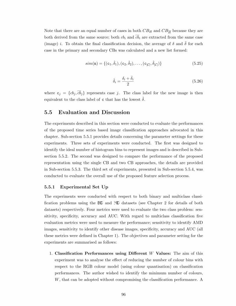
Note that there are an equal number of cases in both CBH and CBH because they are

both derived from the same source; both cbi and cbi are extracted from the same case

(image) i. To obtain the final classification decision, the average of δ and δ for each

case in the primary and secondary CBs was calculated and a new list formed:

sim(n) = {(c1, δ1), (c2, δ2), . . . , (c|C|, δ|C|)} (5.25)

δi =δi + δi

2(5.26)

where cj = {cbj , cbj} represents case j. The class label for the new image is then

equivalent to the class label of c that has the lowest δ.

5.5 Evaluation and Discussion

The experiments described in this section were conducted to evaluate the performances

of the proposed time series based image classification approaches advocated in this

chapter. Sub-section 5.5.1 provides details concerning the parameter settings for these

experiments. Three sets of experiments were conducted. The first was designed to

identify the ideal number of histogram bins to represent images and is described in Sub-

section 5.5.2. The second was designed to compare the performance of the proposed

representation using the single CB and two CB approaches, the details are provided

in Sub-section 5.5.3. The third set of experiments, presented in Sub-section 5.5.4, was

conducted to evaluate the overall use of the proposed feature selection process.

5.5.1 Experimental Set Up

The experiments were conducted with respect to both binary and multiclass classi-

fication problems using the BD and MD datasets (see Chapter 2 for details of both

datasets) respectively. Four metrics were used to evaluate the two class problem: sen-

sitivity, specificity, accuracy and AUC. With regard to multiclass classification five

evaluation metrics were used to measure the performance; sensitivity to identify AMD

images, sensitivity to identify other disease images, specificity, accuracy and AUC (all

these metrics were defined in Chapter 1). The objectives and parameter setting for the

experiments are summarised as follows:

1. Classification Performances using Different W Values: The aim of this

experiment was to analyse the effect of reducing the number of colour bins with

respect to the RGB colour model (using colour quantisation) on classification

performances. The author wished to identify the minimum number of colours,

W , that can be adopted without compromising the classification performance. A

96

sequence of values of W was used: 8, 16, 32, 64, 128 and 256. A maximum value

of W = 256 was selected because: (i) the computational complexity increases

when higher values of W are used, and (ii) initial experiments presented in [88]

shows that W > 256 did not produce significant improvement on the overall

classification performance. For comparison, a green channel histogram of length

256 bins was also considered (it was included because the green channel is the

most informative channel of the RGB colour model with respect to retinal image

analysis).

2. Classification Performances using Different Number of Case Bases: The

aim of this experiment was to analyse the performance of the two proposed CBR

approaches; the first used a single CB, while the other used two CBs. Two types

of feature, colour histograms and colour histograms with the optic disc removed,

were used to construct CBs with respect to the first approach, known as CBH

and CBH respectively. For the second approach, primary and secondary CBs as

described in Sub-section 5.4.2.2 were employed. For segmentation of the optic

disc (see Sub-section 5.2.2.1), three parameters, $, ϕ and ρ, have to be defined.

From the literature, the width of the retinal blood vessels (with an average retinal

fundus images size of 550× 600 pixels) ranged from less than a pixel to 12 pixels

[12, 32, 139, 182]. Thus, $ was set to 12 pixels. With respect to the size of the

optic disc, the diameter ranges from 60 to 105 pixels [12, 140, 148]. Therefore,

ϕ = 131 pixels (to ensure all possible candidates are counted in the identification

of the optic disc centre) and ρ = 45 pixels were selected. A sequence of values

for the threshold τ (to determine if a clear “winner” is identified by the primary

case base) was used: 0.01, 0.05 and 0.1.

3. Classification Performances using Different T Values: The aim of the last

experiment was to determine the optimum T value to be used for feature selection

as described in Section 5.3. Recall that the spatial-colour histograms were gen-

erated by tessellating each image into nine regions and representing each region

with an individual colour histogram and then selecting T of these to represent the

image. For this experiment, the spatial-colour histograms were generated using

a set of W values: 32, 64, 128 and 256. The values of T were ranged from 1 to 9.

The warping window size (for the global constraint used with respect to the DTW

as described in Sub-section 5.4.1) was set to 10% of the longest time series as suggested

in [159]. As described in Sub-section 1.6, all the experiments reported in this section

were conducted using 5 repetitions of TCV. With respect to CBR using a single a CB,

if more than one cb with different class labels have identical δ values, the next closest

cb was taken into account and a voting mechanism used to determine a winner. The

software code to extract the image features, feature selection and classification of the

97

images were designed using Matlab. All experiments were performed using 1.86GHz

Intel(R) Core(TM)2 PC with 2 GB RAM.

5.5.2 Experiment 1: Comparison of Classification Performances usingDifferent W Values

The results of experiments directed at comparing the classification performance using

colour histograms with different numbers of bins, W , is presented and discussed in this

sub-section. Table 5.1 and 5.2 show the results produced using the BD and MD datasets.

The column labels in Table 5.1, starting from the left-hand side, should be interpreted as

follows: (i) W indicates the number of histogram bins, (ii) “Sens” is the sensitivity, (iii)

“Spec” is the specificity, (iv) “Accuracy” is the classification accuracy and (v)“AUC” is

the Area Under the receiver operating Curve (AUC) value. In Table 5.2, the columns

labelled “Sens-AMD” and “Sens-other” represent the sensitivity with respect to the

identification of AMD and other disease images respectively. In each column, two

values are recorded, each of which correspond to the average and standard deviation (in

brackets) of the results generated using five sets of Ten-fold Cross Validation (TCV).

The highest value obtained for each evaluation metric is indicated in bold font. All

results were produced using colour histograms extracted from the RGB colour model

for each image with the number of different colours reduced to W colours, except for

the results in the last row in the tables where the results were generated using only a

green channel histogram of length 256 bins.

Table 5.1: Average classification results obtained using CBH , different W values andthe BD dataset

W Sens (%) Spec (%) Accuracy (%) AUC (%)

8 71.1(1.3) 58.5(0.5) 66.3(0.8) 75.7(0.6)16 64.4(1.0) 60.1(0.7) 62.8(0.8) 77.7(0.7)32 70.9(1.3) 56.2(1.3) 65.4(0.7) 76.5(0.4)64 66.7(1.5) 63.6(1.5) 65.5(1.1) 77.7(0.4)128 69.3(2.4) 55.0(1.5) 64.0(1.5) 74.7(0.8)256 74.0(1.5) 57.4(1.5) 67.8(0.6) 73.9(0.8)

green-256 60.4(1.7) 55.6(1.4) 58.6(1.5) 82.3(0.7)

From Table 5.1 where the BD dataset was used, it can be seen that the best sen-

sitivity (74.0%), specificity (63.6%) and accuracy (67.8%) values were generated using

colour histograms extracted from all three colour channels combined (after colour quan-

tisation). Both the best sensitivity and accuracy were obtained using W = 256, while

the best specificity was produced when W = 64. The individual green channel his-

togram produced the best AUC of 82.3%. Considering the results produced using the

MD dataset presented in Table 5.2, the best sensitivity of 57.0% and the highest accu-

racy of 50.2% for AMD images identification were achieved using W = 256. The best

98

Table 5.2: Average classification results obtained using CBH , different W values andthe MD dataset

W Sens-AMD (%) Sens-other (%) Spec (%) Accuracy (%) AUC (%)

8 45.1(1.2) 39.8(1.8) 43.5(1.0) 42.7(0.7) 65.4(0.3)16 42.1(1.4) 48.2(1.7) 44.2(0.9) 44.7(0.8) 69.4(0.4)32 51.9(0.9) 38.4(2.7) 46.7(0.4) 46.2(1.1) 70.6(0.6)64 52.2(2.8) 45.6(3.0) 47.3(2.9) 48.8(1.4) 72.7(0.9)128 49.5(1.9) 42.9(1.1) 37.9(1.4) 44.5(0.9) 72.8(0.4)256 57.0(2.0) 46.2(1.1) 43.9(2.4) 50.2(0.6) 71.2(0.1)

green-256 44.0(1.3) 64.3(7.6) 29.5(3.2) 47.2(1.9) 70.7(1.2)

recorded sensitivity for the identification of other disease was 64.3% using green channel

histograms. Other best results (specificity and AUC) recorded were 47.3% (W = 64)

and 72.8% (W = 128) respectively. From the experiments, it can be summarised that

most of the best results were achieved using 64 ≤W ≤ 256.

5.5.2.1 Discussion of Experiment 1 Results

Observation of the results obtained using the two class dataset, BD, presented in Table

5.1 indicates that comparable results (between different values of W ) with respect to

accuracy and AUC were produced using histograms generated using all three colour

channels (the accuracy and AUC value obtained were greater than 60% and 70% re-

spectively). The green channel histogram produced the lowest accuracy of 58.6%, but it

performed the best with respect to AUC (82.3%). The results generated across the dif-

ferent sets of TCV runs indicated that consistent results were produced, with standard

deviations of less than 2% for accuracy and less than 1% for AUC.

The results generated from the multiclass dataset, MD, presented in Table 5.2 show

that the overall accuracy is low (the best was just above 50%). Better AUC values

were however produced (greater than 65% for all values of W ) with a recorded best of

72.8%. Inspection of the standard deviations demonstrated that similar accuracy and

AUC results were produced across the different TCV runs, with a standard deviation

of less than 2% for both metrics. Note that CBH was used in these experiments.

The results shown in both tables indicate that the histograms extracted from all

three RGB channels, combined and quantised to W colours, produced better overall

results than using histograms generated from the green channel alone. The suggested

explanation for this results is that histograms representing all channels are more in-

formative, and therefore more discriminative (in the context of image classification),

than the green channel histogram alone. With respect to the W parameter, the results

clearly indicate that the higher the W value, up to W = 256 in the reported exper-

iments, the better the classification accuracy, with the exception of W = 128 where

a slight drop in accuracy was observed compared to W = 64. A similar pattern can

99

be observed with respect to the AUC values, where the AUC values produced were

better when the length of the histograms was increased up to W = 128. This was to

be expected as low numbers of colour bins will tend to group different coloured pixels

into the same bin, and consequently reduce the discriminatory power of the colour rep-

resentation. However, as stated before, increasing the value of W resulted in a higher

computational cost with minimal improvement in classification performances (less than

2% for accuracy and AUC). Thus, the maximum value of W was limited to 256 (note

that the original number of different colours produced by the RGB colour model is

16,777,216 as stated in Sub-section 5.2.1). The presented results show that:

1. Using the BD dataset, the best classification accuracy and AUC were 67.8% (W =

256) and 82.3% (using the green channel histograms) each.

2. Using the MD dataset, the best classification accuracy and AUC were 50.2%

(W = 256) and 72.8% (W = 128) respectively.

3. The selection of parameter W did affect the classification performances whereby

W ≥ 32 tended to produce better overall (accuracy and AUC) results.

4. Using all three RGB channels combined as features produced a better performance

overall than when using the green channel alone.

5. Performance is relatively stable, as the recorded standard deviation is small (less

than 2% for both BD and MD datasets).

6. Better results were produced using the two class dataset, BD.

Based on the above findings, the histograms used in the following experiments were

extracted using all three RGB channels with 32 ≤W ≤ 256.

5.5.3 Experiment 2: Comparison of Classification Performances usingDifferent Numbers of Case Bases

The results of experiments presented in this sub-section compared the performances

of image classification using a single CB and two CBs. To achieve this, two sets of

experiments were conducted. The first set using CBH only (single CB), while the

second used CBH and CBH combined (two CBs) as described in Sub-section 5.4.2.2.

Tables 5.3 and 5.4 show the results produced from the experiments using a single

CB. For comparison purpose, the results of using CBH , as presented in the foregoing

sub-section, are also included in the tables. The results generated using two CBs are

presented in Tables 5.5 and 5.6.

The average classification results presented in Tables 5.3 and 5.4 allow for a compar-

ison of the performance using CBH and CBH (this has been presented and discussed

in sub-section 5.5.2). The results presented in Table 5.3, obtained using the dataset

100

Table 5.3: Average classification results obtained using CBH and CBH separatelyapplied to the BD dataset

WSens (%) Spec (%) Accuracy (%) AUC (%)CBH CBH CBH CBH CBH CBH CBH CBH

3269.1 70.9 54.6 56.2 63.6 65.4 73.8 76.5(1.1) (1.3) (1.1) (1.3) (1.0) (0.7) (0.7) (0.4)

6476.0 66.7 55.7 63.6 68.4 65.5 76.5 77.7(1.2) (1.5) (2.0) (1.5) (1.2) (1.1) (0.7) (0.4)

12872.2 69.3 60.1 55.0 67.7 64.0 72.2 74.7(0.9) (2.4) (0.7) (1.5) (0.6) (1.5) (1.2) (0.8)

25673.4 74.0 58.6 57.4 67.9 67.8 69.6 73.9(1.4) (1.5) 1.6 (1.5) (0.4) (0.6) (1.1) (0.8)

Table 5.4: Average classification results obtained using CBH and CBH separatelyapplied to the MD dataset

WSens-AMD (%) Sens-other (%) Spec (%) Accuracy (%) AUC (%)CBH CBH CBH CBH CBH CBH CBH CBH CBH CBH

3255.2 51.9 41.5 38.4 42.1 46.7 47.3 46.2 69.6 70.6(1.0) (0.9) (2.8) (2.7) (0.8) (0.4) (0.7) (1.1) (0.5) (0.6)

6459.0 52.2 37.9 45.6 40.7 47.3 47.4 48.8 71.2 72.7(0.8) (2.8) (1.5) (3.0) (2.2) (2.9) (0.6) (1.4) (0.6) (0.9)

12850.9 49.5 39.0 42.9 45.0 37.9 45.6 44.5 70.8 72.8(1.6) (1.9) (1.4) (1.1) (2.1) (1.4) (0.6) (0.9) (0.2) (0.4)

25657.8 57.0 41.4 46.2 47.3 43.9 49.8 50.2 68.7 71.2(1.6) (2.0) (1.1) (1.1) (2.8) (2.4) (0.9) (0.6) (0.4) (0.1)

101

Table 5.5: Average classification results obtained using two CBs (CBH and CBH com-bined) and the BD dataset

τ W Sens (%) Spec (%) Accuracy (%) AUC (%)

0.01

32 70.5(1.2) 55.4(1.3) 64.9(0.4) 76.3(0.6)64 68.3(1.4) 61.8(1.3) 65.8(1.0) 77.5(0.3)128 69.5(2.1) 57.2(1.5) 64.9(1.2) 74.4(0.8)256 74.3(1.7) 57.2(1.5) 67.9(0.7) 73.6(0.8)

0.05

32 68.3(0.9) 55.8(2.2) 63.6(0.7) 75.9(0.6)64 68.5(1.3) 61.2(1.3) 65.8(1.0) 78.0(0.7)128 70.9(1.3) 59.1(1.1) 66.5(0.9) 73.9(0.9)256 74.4(1.6) 59.2(2.4) 68.7(0.9) 73.1(1.1)

0.1

32 69.5(0.6) 56.8(2.0) 64.8(0.6) 76.4(0.7)64 70.0(1.4) 60.4(1.0) 66.4(1.0) 77.9(0.4)128 71.7(1.2) 59.7(1.1) 67.3(0.8) 74.0(1.1)256 74.5(1.6) 60.4(1.4) 69.3(0.5) 73.2(1.4)

BD, show that CBH produced the best sensitivity and accuracy (76.0% and 68.4%),

while CBH performed better with respect to specificity and AUC (63.6% and 77.7%).

For the multiclass dataset MD the generated results are shown in Table 5.4, CBH per-

formed better with respect to two of the evaluation metrics, sensitivity for AMD images

(59.0%) and specificity (47.3%). The best sensitivity to identify other diseases, overall

accuracy and AUC were 46.2%, 50.2 % and 72.8% respectively, produced using CBH .

The performance of the proposed two CBs image classification approach is presented

in Tables 5.5 and 5.6. The left-most column in the tables represents the threshold, τ ,

that was used to determine if the secondary CB, CBH , need to be consulted to classify

an image (where the classifier failed to identify a clear winner using the primary CB,

CBH). For dataset BD the results are shown in Table 5.5, the best sensitivity and

accuracy of 74.5% and 69.3% respectively, were obtained using τ = 0.1 and W = 256.

The best specificity was 61.8% (τ = 0.01 and W = 64) and AUC was 78.0% (τ = 0.05

and W = 64). As shown in Table 5.6, the best sensitivity for AMD identification and

AUC obtained using dataset MD were 56.9% and 73.6%. Both were achieved when τ

was set to 0.01. The other best results were: (i) a sensitivity to identify retinal images

with other disease of 45.3%, (ii) a specificity of 48.8% and (iii) an accuracy of 49.8%.

These results were produced when τ was set to 0.1.


Similar to the results discussed in Sub-section 5.5.2, the application of the proposed

approaches (single and two CBs) on the two class problem (dataset BD) produced

better results than when using multiclass (dataset MD). This is to be expected as the

probability of a correct prediction is significantly reduced given a multiclass problem.

102

Table 5.6: Average classification results obtained using two CBs (CBH and CBH com-bined) and the MD dataset

τ W Sens-AMD (%) Sens-other (%) Spec (%) Accuracy (%) AUC (%)

0.01

32 51.8(0.9) 38.6(2.5) 45.5(1.5) 45.8(0.9) 70.7(0.4)64 50.3(1.5) 42.8(1.2) 47.8(1.9) 47.2(0.6) 73.6(0.1)128 49.6(1.8) 43.8(1.2) 39.9(1.6) 45.3(0.7) 73.0(0.5)256 56.9(1.9) 44.6(1.6) 43.7(2.2) 49.6(0.7) 71.2(0.2)

0.05

32 51.5(0.7) 40.1(1.9) 48.6(2.5) 47.0(1.1) 70.9(0.4)64 51.6(2.2) 44.5(1.4) 48.4(1.4) 48.4(0.9) 73.2(0.4)128 49.7(1.5) 42.2(2.0) 43.2(2.1) 45.7(0.8) 72.9(0.4)256 56.4(1.9) 40.8(1.0) 45.7(3.1) 48.6(0.7) 70.6(0.3)

0.1

32 52.0(1.0) 37.7(2.5) 48.2(2.5) 46.2(1.0) 71.1(0.4)64 54.1(1.4) 45.3(1.2) 48.8(1.5) 49.8(0.8) 73.0(0.3)128 50.7(1.7) 41.3(2.1) 44.2(2.1) 46.1(0.8) 72.4(0.3)256 55.6(2.0) 41.4(1.2) 46.3(2.7) 48.6(0.7) 70.5(0.3)

For the two class problem, the generated accuracies and AUCs were both greater than

60% and 70% each for all parameter settings used with respect to both approaches.

For the multiclass problem, low accuracies were produced (less than 55%) while higher

AUCs were generated (greater than 65%) on the single CB approach. For the two CBs

approach (see Table 5.6), the AUC values produced improved to 73.6% compared to

when a single CB was used. However, the comparison also shows that the accuracy

was negatively affected as it was decreased to 49.8% when using the two CBs. With

regard to the type of features used, CBH produced the best accuracy using the BD

dataset, and both accuracy and AUC for the MD dataset (as shown in Table 5.3 and

5.4). The consistency of the results across the different sets of TCVs was good, with

respect to accuracy and AUC. The standard deviations using either the single or two

CBs approach were less than 1.5% for both accuracy and AUC.

The results presented can be summarised as follow:

1. Using the BD dataset, the best classification accuracy and AUC were 69.3% and

78.0% (both were produced using the two CBs approach).

2. Using the MD dataset, the best classification accuracy and AUC were 50.2% (using

CBH) and 73.6% (using the two CBs approach).

3. The two CBs approach tends to performed better than the single CB approach

when using the BD dataset. However, the two CBs approach incurred higher

computational cost.

4. With regard to the CBs used, better performances were likely to be generated

using CBH than CBH .

103

Based on these results, only colour histograms were used as the base with which

to generate spatial-colour histograms with respect to experiment 3 reported in the

following sub-section.

5.5.4 Experiment 3: Comparison of Performances using Different Val-ues of T

The results with respect to experiment 3 presented in this sub-section were used to

analyse the effect of using various T values (recall that the T value was used to de-

termine the number of regions in an image to be considered when constructing time

series). T = “All” indicates that all features (regions) were used for classification. Ta-

bles 5.7 and 5.8 show the classification performances generated using CBH

, a case base

comprised of spatial-colour histograms, when applied to datasets BD and MD respec-

tively. The second column from the left-hand side, with label T , indicates the number

of regions involved in the generation of the histograms. Note that when W = 256 the

selected T values range between 1 and 5 (1 ≤ T ≤ 5). These values were chosen because

inspection on the results produced with W < 256 indicated that the results tended to

either: (i) decreased when T > 5, or (ii) produce only a slight classification accuracy

improvement at the cost of significantly higher computational cost. Thus, the decision

was made to stop the classification process for W = 256 when T > 5.

For the two class problem (Table 5.7), the best recorded values, for each evaluation

metric used, was as follow: (i) a sensitivity of 76.1% (when T = 7 and W = 32), (ii) a

specificity of 64.1% (when T = 8 and W = 64), (iii) an accuracy of 68.4% (when T = 6

and W = 64), and (iv) an AUC of 73.5% (when T = 1 and W = 128). All the best

results were produced using W < 256. The highest classification performances, with

respect to both accuracy and AUC, were generated using T ≤ 7 for all values of W .

With regard to the multiclass problem (Table 5.8), the best results for each evaluation

metrics were as follow: (i) a sensitivity to identify AMD images of 57.9% (when T = 7

and W = 32), (ii) a sensitivity to identify other disease images of 51.8% (when T =

All), (iii) a specificity of 50.5% (when T = 6), (iv) an accuracy of 52.4% (when T = 6)

and (v) an AUC of 72.7% (when T = 3). These best results, except the sensitivity

value to identify AMD images, were produced using W = 64. For all values of W , it

may be observed that most of the classification performances, with respect to accuracy

and AUC, increased when higher values of T was used up to T = 6. This is reflected

by the results in the table whereby the highest accuracy and AUC for each W were

achieved using T ≤ 6.


Inspection of Tables 5.7 and 5.8 show that the proposed approach performed better

when applied to the two class problem. As shown in Table 5.7, the generated accuracies

104

Table 5.7: Average classification results obtained using CBH

, different T values andthe BD dataset

W T Sens (%) Spec (%) Accuracy (%) AUC (%)

32

1 70.6(3.9) 50.5(4.8) 63.1(3.7) 71.6(2.0)2 65.9(1.9) 57.6(4.3) 62.8(2.1) 73.2(0.6)3 67.9(1.3) 54.1(1.5) 62.7(1.0) 70.5(0.5)4 69.8(0.9) 56.3(4.2) 64.8(2.1) 71.7(1.2)5 72.9(1.3) 55.7(2.8) 66.5(1.3) 72.6(0.6)6 75.1(1.5) 55.2(2.6) 67.7(1.2) 71.9(0.6)7 76.1(0.8) 55.1(2.4) 68.3(1.2) 71.6(0.3)8 73.8(1.0) 54.3(2.2) 66.5(1.0) 72.0(0.4)All 74.5(1.6) 55.2(1.7) 67.3(0.8) 71.8(0.9)

64

1 72.0(3.2) 54.0(2.2) 65.3(2.5) 72.1(0.7)2 66.7(3.3) 55.0(3.8) 62.3(2.6) 70.6(2.3)3 72.4(1.5) 57.9(3.9) 67.0(1.9) 71.1(1.1)4 68.9(2.9) 57.9(2.4) 64.8(2.0) 71.6(0.7)5 71.7(1.6) 60.8(2.4) 65.8(4.8) 71.0(1.3)6 72.3(1.5) 61.8(2.8) 68.4(0.9) 70.9(1.3)7 67.1(1.9) 61.7(2.5) 65.0(0.3) 70.5(1.5)8 69.4(0.9) 64.1(2.7) 67.4(0.7) 71.5(1.5)All 70.4(1.8) 60.9(2.2) 66.8(0.7) 71.0(1.2)

128

1 75.8(1.2) 50.7(0.9) 66.4(1.0) 73.5(0.8)2 69.2(2.0) 49.1(0.7) 61.7(1.1) 72.0(1.0)3 71.0(2.0) 52.8(2.7) 64.2(1.5) 72.2(1.8)4 73.2(1.7) 54.0(2.4) 66.1(0.7) 71.0(1.2)5 72.4(1.5) 53.9(2.2) 65.5(0.8) 70.5(1.5)6 70.3(2.5) 53.2(2.9) 63.9(0.8) 70.5(1.4)7 70.3(1.6) 56.2(3.1) 65.0(1.2) 70.6(1.3)8 71.0(1.2) 58.4(3.4) 66.3(1.4) 72.1(1.5)All 70.8(1.8) 57.7(1.3) 65.9(1.5) 72.2(1.4)

256

1 68.1(2.2) 52.9(1.7) 62.4(1.4) 66.2(2.1)2 67.2(1.5) 54.7(2.8) 62.5(0.8) 65.2(2.1)3 65.4(4.7) 55.1(3.7) 61.5(3.4) 65.5(1.2)4 64.1(2.0) 56.9(2.8) 61.3(0.7) 66.4(1.6)5 63.9(4.1) 54.8(2.7) 60.5(3.3) 66.2(1.5)

105

Table 5.8: Average classification results obtained using CBH

, different T values andthe MD dataset

W T Sens-AMD (%) Sens-other (%) Spec (%) Accuracy (%) AUC (%)

32

1 49.1(4.9) 42.5(2.9) 38.0(5.4) 44.1(2.0) 69.1(0.8)2 48.1(2.6) 39.6(3.0) 47.1(2.4) 45.0(1.5) 70.2(0.9)3 50.8(2.0) 40.2(2.7) 48.5(2.2) 46.6(0.7) 69.7(0.3)4 53.7(1.4) 41.9(1.8) 45.9(2.0) 47.8(0.6) 69.1(0.4)5 55.2(1.2) 45.4(0.9) 48.9(2.2) 50.4(0.3) 69.0(0.5)6 57.9(2.6) 43.9(1.8) 48.4(2.6) 50.9(1.2) 68.2(0.6)7 57.9(1.5) 44.1(1.0) 48.4(2.7) 50.9(1.3) 67.6(0.3)8 53.5(1.4) 43.6(1.2) 46.0(3.2) 48.3(0.9) 67.5(0.4)All 49.1(7.7) 35.4(3.9) 50.0(2.8) 44.8(3.9) 66.0(1.9)

64

1 53.0(4.2) 44.9(3.2) 42.6(3.2) 47.7(2.0) 71.6(0.6)2 50.6(3.0) 48.8(1.3) 39.8(2.2) 47.2(1.0) 72.0(0.4)3 54.6(2.2) 48.9(1.0) 46.3(3.2) 50.6(1.5) 72.7(0.6)4 53.8(1.9) 47.6(3.0) 46.8(3.7) 50.0(1.5) 72.3(0.3)5 55.7(1.9) 49.2(1.1) 48.1(4.0) 51.6(1.6) 72.0(0.5)6 57.0(1.9) 48.0(1.4) 50.5(3.1) 52.4(1.3) 70.7(0.2)7 53.4(1.3) 46.5(1.2) 48.8(3.0) 49.9(0.8) 70.9(0.4)8 56.4(1.3) 46.4(1.3) 45.2(2.8) 50.3(0.7) 70.8(0.2)All 56.2(1.9) 51.8(1.1) 43.1(2.5) 51.5(0.4) 70.2(0.4)

128

1 55.6(2.2) 47.7(2.3) 37.8(3.0) 48.6(0.7) 71.0(0.4)2 55.7(2.0) 46.6(1.1) 35.1(1.4) 47.6(1.1) 71.2(0.4)3 54.8(2.0) 43.6(0.7) 39.5(2.3) 47.4(1.2) 70.6(0.7)4 56.6(1.8) 39.7(1.3) 43.6(3.4) 47.8(0.5) 69.6(0.4)5 54.7(1.6) 44.3(3.3) 42.7(3.3) 48.3(1.1) 68.8(0.3)6 54.2(1.0) 43.9(0.8) 42.0(4.8) 47.7(1.3) 68.5(0.4)7 48.9(1.9) 43.7(2.1) 45.5(2.9) 46.4(1.4) 68.4(0.6)8 53.6(1.2) 39.0(1.4) 43.5(2.8) 46.2(0.7) 69.1(0.6)All 54.0(1.9) 40.9(1.0) 43.4(1.5) 46.9(0.9) 69.4(0.5)

256

1 50.8(0.2) 45.2(3.4) 41.3(1.0) 46.6(1.5) 65.5(0.5)2 47.4(3.1) 39.3(3.7) 42.5(2.9) 43.5(2.5) 63.9(0.8)3 48.6(4.8) 41.5(2.4) 44.5(3.5) 45.3(2.2) 63.5(0.5)4 48.3(1.8) 37.8(3.2) 47.8(3.1) 44.6(1.2) 63.7(0.5)5 47.9(2.5) 38.9(3.7) 45.7(3.8) 44.3(1.6) 63.1(1.7)

106

and AUC values were greater than 60% and 65% each for the BD dataset, while the

MD dataset produced accuracies of less than 55% and AUCs of greater than 60%.

Consistent results were produced across the different sets of TCV runs, where the

standard deviation calculated with respect to accuracy and AUC, were less than 5%

and 3% (BD dataset) and less than 3% and 2% (MD dataset) respectively.

The results indicated that by applying feature selection to spatial-colour histograms

improved the classification performances with respect to all evaluation metrics used,

with the exception of the sensitivity to identify other disease images. With regard to

the T values, an ideal T value was not identifiable, though most of the best results

(indicated in bold font) were achieved using T ≥ 3.

Based on the results presented in Tables 5.7 and 5.8, the following summary can be

made (for both the BD and MD datasets):

1. Using the BD dataset, the best accuracy and AUC were 68.4% (W = 64 and

T = 6) and 73.5% (W = 128 and T = 1) respectively.

2. Using the MD dataset, the best accuracy was 52.4% (W = 64 and T = 6) and the

best AUC was 72.7% (W = 64 and T = 3).

3. The highest performance achieved for each value of W , with regard to classifica-

tion accuracy, was recorded using T ≤ 7.

4. T < 4 tends to produce the best AUC value for each W .

5. In terms of the size of spatial-colour histograms (W×T ), the best accuracies were

produced when the length of the spatial-colour histograms was within the range

of 200 to 600 bins.

6. The overall best results with respect to all the evaluation metrics used tended to

be produced using W ≤ 64.

5.5.5 Overall Discussion

A summary of the results generated by the experiments reported in this chapter is

shown in Tables 5.9 and 5.10. In the tables each row represents the results produced by

the best performing parameter settings, with respect to the best classification accuracy

generated. The aim was to compare the performances of the three different proposed

time series based image classification approaches advocated in this chapter. All features

were extracted from the RGB colour model of the images. The left-most column labelled

“Ap.” represents the nature of the CB used to generate the results. The first three rows

present the results generated using a single CB approach, while the last row presents

the results produced using two CBs.

107

Table 5.9: Summary of average best classification results obtained using the proposedapproaches and the BD dataset

Ap. Sens (%) Spec (%) Accuracy (%) AUC (%)

CBH 74.0(1.5) 57.4(1.5) 67.8(0.6) 73.9(0.8)CBH 76.0(1.2) 55.7(2.0) 68.4(1.2) 76.5(0.7)CB

H72.3(1.5) 61.8(2.8) 68.4(0.9) 70.9(1.3)

CBH + CBH 74.5(1.6) 60.4(1.4) 69.3(0.5) 73.2(1.4)

Table 5.10: Summary of average best classification results obtained using the proposedapproaches and the MD dataset

Ap.Sens- Sens-

Spec (%) Accuracy (%) AUC (%)AMD(%) other(%)

CBH 57.0(2.0) 46.2(1.1) 43.9(2.4) 50.2(0.6) 71.2(0.1)CBH 57.8(1.6) 41.4(1.1) 47.3(2.8) 49.8(0.9) 68.7(0.4)CB

H57.0(1.9) 48.0(1.4) 50.5(3.1) 52.4(1.3) 70.7(0.2)

CBH + CBH 54.1(1.4) 45.3(1.2) 48.8(1.5) 49.8(0.8) 73.0(0.3)

As can be seen from Table 5.9, use of CBH produced the best results with respect

to sensitivity and AUC, the best specificity was produced using the CBH

, while the

two CBs approach produced the highest accuracy. From Table 5.10 it can be seen that

the use of CBH

produced the highest results with respect to three of the evaluation

metrics used (sensitivity to identify other disease, specificity and accuracy), while use

of CBH and the two CBs approaches produced the highest sensitivity to identify AMD

images and AUC respectively. Based on the results, histograms that capture both

colour and spatial information, spatial-colour histograms (stored in case base CBH

),

performed the best when the MD dataset was used, while histogram without the optic

disc information performed better with respect to the BD dataset. With regard to

the appropriate number of histogram bins, with respect to the results shown in Tables

5.9 and 5.10, W = 64 tends to produce the best results. Identification of the most

appropriate T value to adopt to obtain the best performance was not conclusive, but

most of the best results were obtained using T ≥ 3. Using two CBs, as shown in

the table, produced comparable results to a single CB approach but with a higher

computational cost.

5.6 Summary

Approaches to classify images using a time series based representation derived from

colour histograms, coupled with TSA and CBR, have been described in this chapter. A

number of different types of colour histograms were advocated, including spatial-colour

histograms that capture both colour and spatial pixel information. Two approaches to

108

classify images using CBR were described, the first used a single CB while the second

utilised two CBs. Evaluation of the proposed approaches resulted in the following main

findings:

1. The single CB approach produced most of the best results compared to the two

CBs approach.

2. Best results were most likely to be produced using W ≤ 64.

3. An ideal value for T was not identifiable though good results tended to be pro-

duced using T ≥ 3.

4. The generated classification results indicated that the utilisation of colour his-

togram as image features, coupled with TSA and CBR, was not sufficient for

multiclass classification (at least in the case of retinal image datasets used in this

thesis).

The following chapter presents a different image representation, founded on a tabu-

lar based image representation, that outperforms the time series approach described in

this chapter. However, the time series representation does provide a benchmark with

which other approaches described later in this thesis can be compared.

109

Chapter 6

Tabular Based ImageRepresentation for ImageClassification

This chapter presents the second proposed image classification method, founded on a

tabular representation, that utilises the basic 2-D array image format. The evaluation

section in the foregoing chapter demonstrated that the combination of colour and spa-

tial information tends to produced better classification performance than when using

colour information alone. Therefore, the proposed tabular representation presented in

this chapter utilised both colour and spatial information to identify image features com-

prised of statistical parameters which can be extracted either directly or indirectly from

the representation. These direct and indirect parameters can be extracted according to

two strategies, either globally from the entire image, or as a result of partitioning the

image to some level of decomposition (d) and extract the parameters on a region by

region basis. We refer to the first strategy (S1) as the non-partitioning strategy and the

second (S2) as the partitioning strategy. In the case of the S2 strategy the number of

parameters will depend on the level of decomposition. In both cases a feature selection

process is applied where the top T features are selected, partly so that the most discrim-

inating parameters are used for the classification and partly so that the overall number

of parameters to be considered is reduced. The rest of this chapter is arranged as fol-

lows. Section 6.1 presents a more detailed overview of the proposed method. Sections

6.2 and 6.3 provide the details of how the parameter extraction and feature selection

processes are conducted. The adopted classification mechanism is described in Section

6.4, while the classification strategy to achieve multiclass classification is considered

in Section 6.5. Section 6.6 discusses the experiments used to evaluate the proposed

method and reports on the results obtained. The evaluation includes consideration of

the most appropriate value for T to be used for both S1 and S2, and the best level of

decomposition (d) to be used with respect to S2. Finally, a summary of this chapter is

given in Section 6.7.

110

6.1 Introduction

As discussed in the literature review (see Sub-section 3.5), the 2-D array image repre-

sentation is the most common method used to represent images in a way that permits

both the general application of learning algorithms and the extraction of statistical

measures for purposes such as image classification. In most cases, the features used

are derived statistically from the colour, texture or shape information. For the work

described in this chapter, only colour and texture information were considered as we

are interested in composition of the entire image and not individual shapes within it.

Two mechanisms for feature extraction were adopted. The first extracts statistical fea-

ture information directly from the 2-D image colour representation. Examples include

colour, histogram and co-occurrence matrix features. The second applies a transform to

the basic colour representation to produce a frequency based representation, from which

features can then be extracted. The Discrete Wavelet Transform (DWT) was used for

this later purpose (an alternative might have been the Discrete Cosine Transform).

Thus the features used with respect to the proposed solution presented in this chapter

were extracted using both the basic and a transformed 2-D array image representations.

As already noted, two alternative tabular based image representation strategies were

adopted: (S1) extraction of features from the whole image, and (S2) partitioning of each

image into equal sized sub-regions and then extracting features from each sub-region.

For S1 the number of extracted features was 15, which comprised various image proper-

ties that encompass colour (6 features), histogram (2 features), co-occurrence matrix (3

features) and wavelet (4 features) based features. For the second strategy, the identical

15 features were generated but from each sub-region of the image. The total num-

ber of possible features in this later case was thus 15 ×R, where R is the number of

sub-regions, which in turn is dictated by the level of decomposition (d). Details of the

features used in the image representation are described in the following section.

6.2 Features Extraction

The fifteen features used in the proposed tabular based image representation may be

categorised as follows:

1. Features generated directly from the pixel colour information con-

tained in the image (six features). The six colour features extracted were

the average values for each of the RGB colour channels (red, green and blue) and

the HSI components (hue, saturation and intensity). These values were computed

directly from the 2-D array colour representation of each image.

2. Features generated from a “colour histogram” representing the colour

information contained in the image (two features). The two histogram

111

based features were: (i) histogram spread and (ii) histogram skewness. Only the

green channel colour histogram was used as this has been demonstrated to be

more informative than the other channels in the context of retina image analysis

[32, 158]. Once extracted, each histogram was normalised with respect to the

total number of pixels of the ROI in the image. The histogram spread (also

known as variance), hspread, and skewness, hskew, were computed as follow:

hspread =1

|h|

|h|∑i=1

(hi − h)2 (6.1)

hskew =1

|h|

|h|∑i=1

(hi − h)3 (6.2)

where |h| is the number of histogram bins, h is the normalised histogram and h

is the normalised histogram mean.

3. Features generated from the co-occurrence matrices representing the

image (three features). A co-occurrence matrix is a matrix that represents im-

age texture information in the form of the number of occurrences of immediately

adjacent intensity values that appear in a given direction P [74, 85]. Figure 6.1

shows an example of a 6×6 image I and its corresponding co-occurrence matrix,

L. To construct L, a position operator, P, has to be defined. Four possible differ-

ent directions can be used to define P: 0◦, 45◦, 90◦ or 135◦ (see Figure 6.2 where X

is the pixel of interest). With reference to the co-occurrence matrix, L, in Figure

6.1, the number of different intensity values is in the range of [0 7], thus a matrix

of 8× 8 size is produced. P is defined as 0◦, which means that the neighbour of a

pixel is the adjacent pixel to its right. As shown in L, the position (2, 1) contains

a value of 2 as there are two occurrences of pixels with an intensity value of 1

positioned immediately to the right of a pixel with an intensity value of 2 (as

indicated by oval shapes in the figure) in I. The same applies to the element (6,

4) of L that holds a value of 1 as there is only one pixel with an intensity value

of 6 with a pixel with an intensity value of 4 immediately to its right in I, and so

on. With respect to the approach described in this chapter, four co-occurrence

matrices (one for each P direction) were generated for each image. Three textural

features were then extracted from each matrix: (i) correlation, (ii) energy and

(iii) entropy:

Correlation: Measure of how correlated a pixel is to its neighbours over the

entire image. The range of values is [-1, 1], corresponding to negative or

positive correlation. Correlation, corr, for a |L| × |L| matrix is defined as:

112

2 3 3 2 1 5

4 2 7 6 0 0

5 7 7 2 2 1

0 7 6 5 6 4

3 3 0 0 0 0

0 0 0 0 0 0

9 0 0 0 0 0 0 1

0 0 0 0 0 1 0 0

0 2 1 1 0 0 0 1

1 0 1 2 0 0 0 0

0 0 1 0 0 0 0 0

0 0 0 0 0 0 1 1

1 0 0 0 1 1 0 0

0 0 1 0 0 0 2 1

Image I Co-occurrence matrix L

0

1

2

3

4

5

6

7

0 1 2 3 4 5 6 7

Figure 6.1: An example of image and its corresponding co-occurrence matrix (P = 0◦)

X 0o

135o

90o

45o

Figure 6.2: Position operator values

113

corr =

|L|∑x=x+1

|L|∑y=y+1

(x− µrow)(y − µcol)Pxyσrowσcol

, σrow 6= 0;σcol 6= 0 (6.3)

where µrow and µcol are the means of the rows and columns of L respectively,

while σrow and σcol are the standard deviations of L computed along its rows

and columns. Pxy is the element (x, y) normalised to the sum of elements of

L.

Energy: Measure of the uniformity of elements of L. The computed value is in

the range of [0, 1], where energy is 1 for a constant image. Energy, E , is

defined as:

E =

|L|−1∑x=1

|L|−1∑y=1

P 2xy (6.4)

Entropy: Measure of the randomness of the elements of L; the computed value

is in the range of [0, 2log2|L|]. Entropy is 0 if all Pxy are zero and maximum

if all Pxy are equal. Entropy, entr, is defined as:

entr = −|L|∑

x=x+1

|L|∑y=y+1

Pxylog2Pxy (6.5)

The average values of corr, E and entr were then computed across the generated

co-occurrence matrices (of different P values) to form the three co-occurrence

based features.

4. Features generated using a wavelet transform (four features). A sin-

gle level 2-D Discrete Wavelet Transform (DWT) was employed to generate the

four wavelet based features used. The features were extracted by computing the

average of four types of DWT coefficient:

(a) Wϕ(j0,m, n).

(b) WHψ (j,m, n).

(c) W Vψ (j,m, n).

(d) WDψ (j,m, n).

The first wavelet based feature (feature 1) is a scale based DWT; while features

2, 3 and 4 correspond to the wavelet response to intensity variations in three

different directions: horizontal, vertical and diagonal respectively. To generate

114

Wϕ(j0,m, n) and W iψ(j,m, n) (i ∈ {H,V,D}), assume an image f(x, y) of size

row × col. The DWTs were then computed as follows [74]:

Wϕ(j0,m, n) =1√

row × col

row−1∑x=0

col−1∑y=0

f(x, y)ϕj0,m,n(x, y) (6.6)

W iψ(j,m, n) =

1√row × col

row−1∑x=0

col−1∑y=0

f(x, y)ψij,m,n(x, y) (6.7)

where j = 0, 1, . . . , J − 1 is the scaling value, m = n = 0, 1, . . . , 2j − 1 are the

translation parameters, ϕj0,m,n and ψij,m,n are the scaling and translation basis

functions respectively. Both functions are defined as [74]:

ϕj0,m,n = 2j/2ϕ(2jx−m, 2jy − n) (6.8)

ψij,m,n = 2j/2ψ(2jx−m, 2jy − n) (6.9)

The 2-D scaling, ϕ(x, y), and translation, ψi(x, y), functions were derived from

their corresponding 1-D functions as follows [74]:

ϕ(x, y) = ϕ(x)ϕ(y) (6.10)

ψH(x, y) = ψ(x)ϕ(y) (6.11)

ψV (x, y) = ϕ(x)ψ(y) (6.12)

ψD(x, y) = ψ(x)ψ(y) (6.13)

The values of ϕ(t) and ψ(t) were determined by the types of wavelet filters used.

In this chapter, the most common Haar wavelet filter was employed and defined

as:

ϕ(t) =

{1, 0 ≤ t < 10, otherwise

(6.14)

ψ(t) =

1 0 ≤ t < 0.5−1 0.5 ≤ t < 10 otherwise

(6.15)

115

The overall feature generation process is illustrated by the block diagram presented

in Figure 6.3. Each of the pre-processed colour images (see Chapter 4 for details of the

image pre-processing method employed in this thesis) was first represented in a 2-D

array form. The size of the array is equivalent to the size of the image it represents;

each element of the array contains a pixel intensity value. The colour based features

were extracted directly from this array. The other categories of feature (histograms, co-

occurrence matrix and wavelet) were extracted from the green channel representation of

the images. Thus, a 2-D array of the green channel image representation was generated

from each image. The colour (green channel) histogram, co-occurrence matrix and

wavelet based features were then extracted from this array. The resulting features were

kept in a tabular form where each column represents a feature, and each row an image.

In the second strategy, where images were partitioned into R sub-regions using

a quad-tree image decomposition technique, the features were generated from each

sub-region. Note that in the context of the work presented in this chapter, the decom-

position of an image will be performed until it reaches a predefined depth, d. Since

quad-trees are more suited to square images, the image size was first expanded so that

both the height and width of the images were identical. In the context of the work

described in this thesis, the dimensions of each retinal image was fixed to 768×768 pix-

els. This was achieved by expanding the images with zero valued pixels. The extracted

feature vectors were then arranged according to the order of the sub-regions that they

represent in an ascending manner, such that the features of the first sub-region formed

the first 15 features, the second sub-region formed the next 15 features, while the Rth

sub-region formed the last 15 features. Figure 6.4 shows the sub-region ordering of an

image using a quad-tree of depth, d = 2. The value of R is thus determined by the

value of d such that R = 4d.

6.3 Features Selection

The next step is to reduce the number of extracted features; the aim being to prune the

feature space so as to increase the classification efficiency (through removal of redundant

or insignificant features) while at the same time maximising the classification accuracy.

A feature selection based method to filter the generated statistical parameters was thus

applied.

The proposed feature selection method comprises a feature ranking strategy based

on the discriminatory power of each feature and selecting the top T . By doing this, only

the most appropriate features were selected for the classification task and consequently a

better classification result could be produced. The feature ranking mechanism employed

used SVM weights to rank features [30]. The main advantage of this approach was

its implementational simplicity and effectiveness in identifying relevant features, as

demonstrated in [30].

116

2-D array colour image

representation

Represent images in 2-D array

Colour image

dataset

Extract colour information features

2-D array green channel image representation

Extract green channel information

Extract colour (green channel) histogram

features

Extract co-occurrence matrix

features

Extract wavelet features

Colour features

Colour histogram features

Co-occurrence

features

Wavelet features

Tabular image representation

Figure 6.3: Block diagram of features extraction steps

Algorithm 1: Feature Ranking using SVM

Data: Training sets F and cResult: Sorted features list sortedF

1 C ← GetParameter(F, c) ; // Find best parameter for SVM

2 listF ← TrainModel(F,C) ; // Get weight of each feature

3 sortedF ← Sort(listF );4 return sortedF

117

0 1

2 3

4 5

6 7

8 9

10 11

12 13

14 15

Figure 6.4: Ordering of sub-regions produced using a quad-tree image decompositionof depth 2

Note that a C-Support Vector Classification (C-SVC) [22, 94] type of SVM was

used in the work described in this thesis. C-SVC solves the optimisation problem as

presented in equation 3.15 (in Chapter 3). For a training set that is linearly separable,

a linear kernel function is used to map the original data into a higher dimensional space

as follows [94]:

K(Xi,Xj) = XTi ·Xj (6.16)

Algorithm 1 [30] describes the feature ranking process. The input, F , is the set

of identified features presented in the form of a feature vector, and the output is a

ranked list of the features, sortedF , sorted according to their weights. The algorithm

commences with the selection of the best penalty parameter, C, for the SVM (the

GetParameter function in line 1). To determine C, a SVM based parameter selection

tool [29], a tool that trains the SVM with various parameter settings and performs

classification on the training set using n-fold cross validation, was applied to the input

set F . A range of c values, such that C = 2c, and F were supplied to the GetParameter

function. The best c value was then identified in the following manner:

1. Split F into training and test sets.

2. Train the SVM using the supplied c value on a linear kernel.

3. Perform classifications on the test set and get the results.

4. Repeat from step 2 until all c values are used.

Steps 1 to 3 of the above process were repeated n times, thus n-fold cross validation.

The C value that produced the highest classification accuracy was then selected as the

parameter for the SVM to generate feature weights (to be used in the ranking) in

the TrainModel function (line 2). The L2-regularised with L2-loss function SVM with a

118

linear kernel (provided in the LIBLINEAR library [54]) was employed (a one-versus-the

rest strategy was utilised for the MD dataset). A linear kernel was chosen for the ranking

of the features due to its superiority in selecting significant features as reported in [30].

The resulting model, listF , contains a weight value for each feature. With respect

to the MD dataset, three weight values for each feature were computed (as there are

three classes that exist in the dataset). The average weight of each feature was then

calculated and used to sort the features in descending order, sortedF (function Sort in

line 3). The feature selection process was concluded by selecting the top T features

from sortedF for the classification task. The identified features were then arranged

in a tabular form that defined the feature space of interest. Each row represents an

individual image, and its corresponding features are defined by the columns.

6.4 Classifier Generation

The final stage of the solution proposed in this chapter is the classification stage. The

nature of the tabular feature space representation permits the application of many dif-

ferent classification algorithms. In the context of the work described in this chapter,

three classification algorithms were used: instance based k-NN, parameterless Naıve

Bayes (NB) and a SVM. k-NN was selected because of its simplicity. NB was selected

because: (i) it has been shown to work well on various types of dataset and is com-

parable (with regard to reported classification accuracy with respect to a variety of

applications) to other classification techniques such as decision trees [46], and (ii) it

does not require user defined parameters (unlike k-NN and SVM). SVM was selected

because it is recognised as one of the most effective classification methods in machine

learning. To implement NB, a package available in Weka [201] was used. For the SVM,

a package available in the LibSVM [29] library with the C-SVC type of SVM and RBF

kernel were employed, thus a C parameter has to be defined. With respect to the RBF

kernel, an additional parameter, γ, has to be identified. A similar process to parameter

selection as in the GetParameter function in Algorithm 1 was employed. Instead of

identifying only the best C, the function was also used to find the best γ value. Two

sets of c and g values, such that C = 2c and γ = 2g were supplied. The SVM was then

trained. The n-fold cross validation was used for every pair of C and γ. The pair of C

and γ values that produced the best classification result were selected as the parameters

with which to train the SVM classifier (with a RBF kernel). k-NN performs classifica-

tion by identifying the closest k neighbours (in the training sets) for each record in the

test data. A voting mechanism is then used to determine class label of a new record.

With respect to the work described in this thesis, the distance between a test image, u,

and a training image, v, was computed using a weighted Euclidean distance formula:

119

d(u, v) =

√√√√ A∑i=1

wi(ui − vi)2 (6.17)

where w is the weight of an individual feature (attribute) computed by the feature

ranking algorithm as described in Section 6.3.

6.5 Classification Strategies for Multiclass Classification

The solutions proposed in this thesis were evaluated on binary and multiclass image

classification problems. With respect to the latter, the number of different classes was

three (see Chapter 1 Section 1.1). Some classification techniques are able to perform

classification on multiclass problems directly, examples are k-NN and decision trees.

Some however requires a mechanism to reduce the multiclass problem to binary clas-

sification problem. Two such mechanisms are “one-against-all” and “one-against-one”

[95, 133, 164].

In the one-against-all strategy the generated classifiers are designed to distinguish

images belonging to one class from all remaining classes. The number of “base” clas-

sifiers required is equivalent to the number of classes. Thus three base classifiers are

required to solve the M = 3 class image classification problem: (i) class 1 against the

rest, (ii) class 2 against the rest, and (iii) class 3 against the rest. Thus, each classi-

fier corresponds to the probability of an image, X , belonging to one of the predefined

classes. A record X is allocated to a class according to a maximum scoring (probability)

system.

The one-against-one strategy (also called all-pairs or all-against-all) performs a

pairwise comparison between two classes at a time. Thus, for an M class problem, to

classify an image, X , M(M−1)2 base classifiers are required for the classification. For

example, a three (M = 3) class problem will require three classifiers, each performing

a pairwise class comparison: (i) class 1 against class 2, (ii) class 1 against class 3

and (iii) class 2 against class 3 respectively. Each classifier will predict a class for

X . To decide which class X belongs to, two strategies can be applied [29, 95]: (i)

voting or (ii) probability estimate. Voting mechanisms determine the class of X such

that the vote for class 1 is increased by one if X is classified as class 1 by any of

the relevant classifier. The class with the most votes is the winner. Classification

based on probability estimates, on the other hand, uses the estimated pairwise class

probabilities to generate the overall probability for each class; in this case the class that

has the highest computed probability is the winner.

120


This section describes the experimental setup for the experiments conducted to evaluate

the tabular approach proposed in this chapter, and also discusses the results. Details of

the experimental settings are presented in Sub-section 6.6.1. Two sets of experiments

were conducted. The first to compare strategy S1 with S2, and the second to evaluate

the use of the proposed feature selection process. The first is described in Sub-section

6.6.2, and the second in Sub-section 6.6.3.


To evaluate the tabular based image representation presented in this chapter it was

applied to the retinal image datasets described in Chapter 2. Two sets of data were

derived from the image data set; the first, BD, consists of AMD and normal images

only; while the second, MD, consists of AMD and normal images as well as other disease

images. The former was used to evaluate the performance of the proposed approaches

in terms of binary classification, while the latter was used to conduct evaluation in

terms of multiclass classification. Four evaluation metrics were used to measure the

classification performance using the BD dataset; sensitivity, specificity, accuracy and

AUC. With respect to the MD dataset, five evaluation metrics were used; sensitivity to

identify AMD images, sensitivity to identify other disease images, specificity, accuracy

and AUC (see Chapter 1 for details). The objectives of the two sets of experiments

were as follows:

1. Identification of the feature extraction strategy that gives the best

performance: To compare the operation of the non-partitioning (S1) and parti-

tioning (S2) strategies described in Section 6.2 using various classifier generators.

For the second strategy, the depths of image decomposition, d, were set to 2, 3

and 4. Thus four variations of the tabular representation were compared. The

size of the feature space for the first (non-partitioning) strategy was 15. For the

second strategy, the feature space size, using d = 2, 3 and 4, were 240, 960 and

3840 respectively.

2. Number of selected features (T ): To observe and determine the most appro-

priate setting for the T parameter, the thresholds used to define the minimum

number of features required to produce the best classification results. Two sets of

T values were used, one for each feature extraction strategy. For the first strategy,

T was set to a minimum value of 8 and maximum of 14, with a step interval of

1. For the second strategy, the values of T was set to 50, 100, 200, 400, 1000 and

2000.

121

Prior to feature selection and classification, the feature vectors were scaled to within

the range [-1, +1]. This was done to avoid features that have a more extensive range

dominating over features that do not, and consequently exert a greater influence over

the classification performance [94]. Some parameters needed to be defined for the

feature extraction process as described in Section 6.2. For the histogram based features,

the number of bins, h, was set to 256 (the original number of different intensity levels

of a true colour image). To generate the co-occurrence vectors, the size of the co-

occurrence matrix must neither be too small (to avoid loss of information) nor too

large (to reduce computational cost). In this chapter, the number of intensity levels

was reduced to 32, scaled to the minimum and maximum intensity values contain in the

image. Thus, the dimensional size, |L| × |L|, of the co-occurrence matrix was 32× 32.

Finally, with respect to wavelet features, a single level wavelet transform (J = 1) was

employed.

As mentioned in Sections 6.3 and 6.4, a parameter selection tool [29] was employed

to find the best C and γ values (for the SVM classifier) for each generated feature

space. To achieve this, a range of c and g values (only c values were required for

Section 6.3) were applied; −5 ≤ c ≤ 15 and −15 ≤ g ≤ 3 respectively, with a step of

2 between intervals. This process was repeated five times (five-fold cross validation).

A pair of C and γ value, such that C = 2c and γ = 2g, that produced the best

classification accuracy (with regards to the parameter selection process) was selected

for the classification process. For k-NN, the number of neighbours, k, was set to

a minimum of 1 and maximum of 20. With respect to the multiclass classification

strategy, a one-against-one method was used with respect to the SVM classifier as this

method has been proven to be competitive for SVM based classification [95]. The

strategy to determine the winner using probability estimates as described in [204] was

applied. For Naıve Bayes (NB), the computed posterior class probability was used

directly to determine the class label. With respect to k-NN, a voting mechanism was

employed whereby the class that occurs the most frequently in the k closest neighbours

of a test image is declared the winner. In case of ties, the average distance of the

tied classes to the test image was used to determine the winner. Note that all results

shown were obtained using the average of sequences of results produced using five sets

of TCV (details can be found in Sub-section 1.6). The results shown are generated

by calculating the average and standard deviation of the results obtained from the

five sets of TCV. The code to extract the image features was designed using Matlab.

Standard classification techniques available in Weka were used to perform the image

classification. All experiments were conducted using 1.86GHz Intel(R) Core(TM)2 PC

with 2 GB RAM.

122

6.6.2 Experiment 1: Comparison of Classification Performances usingStrategy S1 and S2

The results of experiments directed at comparing the partitioning (S1) and non-parti-

tioning (S2) strategies are presented in this sub-section. The proposed approaches were

evaluated using the BD and MD datasets. Sub-section 6.6.2.1 and 6.6.2.2 present the

results.

6.6.2.1 Classification Results using the BD Dataset

To show the performances of image classification using various k values for k-NN, with

respect to the accuracy and AUC evaluation metrics, plots as shown in Figure 6.5

was utilised. To compare the performance of different classification techniques, the

classification results obtained using k-NN, NB and SVM, as shown in Tables 6.1, 6.2

and 6.3 respectively, were used. Note that Table 6.1 presents results based on the best

accuracy achieved by each strategy only, while Tables 6.2 and 6.3 include the full results

produced by the corresponding classification techniques.

The classification performances achieved using five TCV runs when applying the

proposed tabular representations to the retinal image data (BD dataset) and building

the desired classification using k-NN is shown in Figure 6.5. Figure 6.5(a) shows plots

of values for k against accuracy. Figure 6.5(b) shows plots of values for k against AUC

values. Recall that three different depths of decomposition were used with respect to

S2: 2, 3 and 4. From the figure, the best accuracy and AUC produced using S1 were

79.4% (using k = 16) and 83.1% (using k = 15 and 17). Other evaluation metrics

obtained for S1 (not shown in the figure) were sensitivity of 88.9% (using k = 6) and

specificity of 72.2% (using k = 9). With respect to strategy S2, the best accuracy

and AUC were 76.8% (using d = 2 and k = 3) and 83.1% (using d = 2 and k = 14)

respectively. The best sensitivity for S2 was 95.9% (using d = 3 and k = 20) while

the best specificity was 74.3% (using d = 4 and k = 1 and 2). S1 produced the best

performance with respect to accuracy for all k when 3 ≤ k ≤ 20.

Tables 6.1, 6.2 and 6.3 present the classification results obtained using k-NN, NB

and SVM respectively on the BD dataset. Two values are recorded in each column, cor-

responding to the average and standard deviation (in bracket) of the results obtained.

The column labels should be interpreted as follow: (i) “Strategy” defines the feature

extraction strategy used to generate the results, (ii) “Sens” is the classifier sensitivity,

(iii) “Spec” is the average classifier specificity, (v) “Accuracy” is the average accuracy

and (vi) “AUC” is the average AUC value obtained. The best results for each evalua-

tion metric are indicated in bold font, except for results generated using k-NN (shown

in Table 6.1) where only best results (with respect to accuracy) have been selected for

presentation here.

Inspection on the results presented in Table 6.1 and Figure 6.5 show that no single

123

(a)

(b)

Figure 6.5: Comparison of average (a) accuracy and (b) AUC results for image classifi-cation using k-NN and the non-partitioning (S1) and partitioning (S2) strategies usingthe BD dataset

Table 6.1: Average results based on best accuracies for retinal image classificationgenerated using S1 and S2, k-NN and the BD dataset

Strategy Sens (%) Spec (%) Accuracy (%) AUC (%)

S1 87.1(1.6) 66.3(1.7) 79.4(1.7) 83.0(0.3)

S2d2 88.5(0.7) 38.6(3.7) 69.9(1.2) 70.6(1.3)d3 92.8(1.0) 30.3(1.0) 69.5(0.9) 70.2(0.9)d4 79.4(1.5) 72.4(1.2) 76.8(0.9) 81.5(0.6)

124

Table 6.2: Average results obtained using S1 and S2, NB and the BD dataset


S1 64.6(1.4) 76.6(1.5) 69.1(1.0) 76.5(0.8)

S2d2 67.0(0.6) 73.7(0.7) 69.5(0.6) 75.7(0.6)d3 72.3(1.1) 70.5(1.9) 71.6(1.0) 75.6(0.8)d4 76.6(0.8) 63.8(1.5) 71.9(0.7) 74.5(0.4)

Table 6.3: Average results obtained using S1 and S2, SVM and the BD dataset


S1 87.9(1.4) 69.3(2.8) 81.0(1.6) 88.6(1.0)

S2d2 88.4(0.8) 64.7(3.8) 79.5(1.5) 85.3(0.7)d3 88.6(1.2) 69.2(2.1) 81.4(1.1) 86.4(0.9)d4 88.7(0.3) 66.5(2.2) 80.4(0.8) 88.1(0.4)

best k value can be identified. The results for strategy S1 were produced using k = 16,

while for strategy S2 the results were obtained using k = 15 (for S2-d2), k = 8 (for

S2-d3) and k = 3 (for S2-d4). The results also indicate that S1 performed better than

S2 when the k-NN classifier was employed. This pattern of results was not replicated

when NB and SVM classifiers were used, where the S2 strategy was found to produce

the best performances. For the NB classifier, no “best” d value was found. The best

accuracy and AUC, achieved, using strategy S2, were 71.9% (d = 4) and 75.7% (d = 2)

as indicated in Table 6.2. With regard to the SVM classifier, the best accuracy was

recorded using strategy S2 (81.4% using d = 3), while the best AUC was achieved by

S1 (88.6%).

The results using the BD dataset can be summarised as follows:

1. The best classification accuracy and AUC using the BD dataset were 81.4% (strat-

egy S2 and d = 2) and 88.6% (strategy S1). Both were produced using SVM.

2. Strategy S2 produced the best classification accuracy, while S1 produced the best

classification AUC.

3. No single value for k (for k-NN) that produced the best classification results with

respect to both strategies S1 and S2 was identified.

4. The best performing d value was also not conclusive.

6.6.2.2 Classification Results using the MD Dataset

Similar to the foregoing sub-section, the image classification performance using various

k values with k-NN, with respect to the accuracy and AUC evaluation metrics using

the MD dataset, are plotted in Figure 6.6. Tables 6.4, 6.5 and 6.6 show the results

125

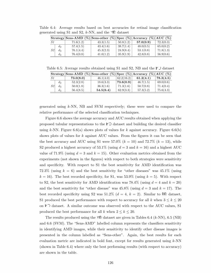
Table 6.4: Average results based on best accuracies for retinal image classificationgenerated using S1 and S2, k-NN, and the MD dataset

Strategy Sens-AMD (%) Sens-other (%) Spec (%) Accuracy (%) AUC (%)

S1 71.6(1.2) 43.3(1.5) 50.8(1.2) 57.0(0.9) 72.3(0.3)

S2d2 57.4(1.5) 43.4(1.6) 38.7(1.4) 48.0(0.5) 65.0(0.2)d3 76.1(4.4) 45.3(2.3) 24.9(8.4) 53.1(0.8) 71.8(1.3)d4 76.4(0.8) 41.0(1.2) 35.9(1.9) 42.8(0.8) 56.9(0.6)

Table 6.5: Average results obtained using S1 and S2, NB and the MD dataset


S1 73.0(8.0) 46.1(4.0) 62.2(16.2) 61.2(4.1) 78.3(4.5)

S2d2 52.3(2.8) 18.6(3.3) 73.6(0.9) 46.7(1.5) 69.0(0.6)d3 50.0(1.8) 36.3(1.6) 71.3(1.6) 50.7(0.8) 71.4(0.4)d4 56.4(8.5) 54.5(6.4) 62.9(3.3) 57.3(5.2) 75.6(4.3)

generated using k-NN, NB and SVM respectively; these were used to compare the

relative performance of the selected classification techniques.

Figure 6.6 shows the average accuracy and AUC results obtained when applying the

proposed tabular representations to the MD dataset and building the desired classifier

using k-NN. Figure 6.6(a) shows plots of values for k against accuracy. Figure 6.6(b)

shows plots of values for k against AUC values. From the figures it can be seen that

the best accuracy and AUC using S1 were 57.0% (k = 10) and 72.7% (k = 13), while

S2 produced a highest accuracy of 53.1% (using d = 3 and k = 16) and a highest AUC

value of 71.9% (using d = 3 and k = 15). Other evaluation metrics obtained from the

experiments (not shown in the figures) with respect to both strategies were sensitivity

and specificity. With respect to S1 the best sensitivity for AMD identification was

72.3% (using k = 6) and the best sensitivity for “other diseases” was 45.1% (using

k = 16). The best recorded specificity, for S1, was 53.9% (using k = 5). With respect

to S2, the best sensitivity for AMD identification was 78.4% (using d = 4 and k = 20)

and the best sensitivity for “other disease” was 45.8% (using d = 3 and k = 17). The

best recorded specificity using S2 was 51.2% (d = 4, k = 2). Similar to BD dataset,

S1 produced the best performance with respect to accuracy for all k when 3 ≤ k ≤ 20

on MD dataset. A similar outcome was observed with respect to the AUC values, S1

produced the best performance for all k when 2 ≤ k ≤ 20.

The results produced using the MD dataset are given in Tables 6.4 (k-NN), 6.5 (NB)

and 6.6 (SVM). The “Sens-AMD” labelled column represents the classifiers sensitivity

in identifying AMD images, while their sensitivity to identify other disease images is

presented in the column labelled as “Sens-other”. Again, the best results for each

evaluation metric are indicated in bold font, except for results generated using k-NN

(shown in Table 6.4) where only the best performing results (with respect to accuracy)

are shown in the table.

126

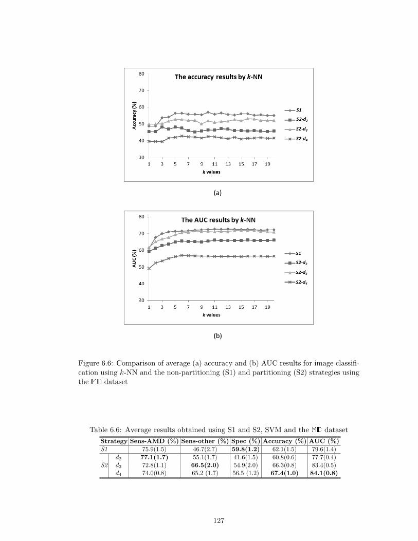
(a)

(b)

Figure 6.6: Comparison of average (a) accuracy and (b) AUC results for image classifi-cation using k-NN and the non-partitioning (S1) and partitioning (S2) strategies usingthe MD dataset

Table 6.6: Average results obtained using S1 and S2, SVM and the MD dataset


S1 75.9(1.5) 46.7(2.7) 59.8(1.2) 62.1(1.5) 79.6(1.4)

S2d2 77.1(1.7) 55.1(1.7) 41.6(1.5) 60.8(0.6) 77.7(0.4)d3 72.8(1.1) 66.5(2.0) 54.9(2.0) 66.3(0.8) 83.4(0.5)d4 74.0(0.8) 65.2 (1.7) 56.5 (1.2) 67.4(1.0) 84.1(0.8)

127

Inspection of the results shown in Table 6.4 (and Figure 6.6) indicated that, similar

to the results produced using the BD dataset, no single best value for k could be

identified. The k-NN results displayed in Table 6.4 were generated using different k

values based on the best accuracy achieved by each strategy and d (for strategy S2

only); the results for S1 were obtained using k = 10, while the results for S2-d2, S2-d3

and S2-d4 were generated using k = 5, 16 and 6 respectively. As noted above, Figure

6.6(a) indicated that strategy S1 performed better than strategy S2 when using k-NN

classification with respect to classification accuracy. This result is corroborated by the

results presented in Table 6.4. A similar pattern was produced using NB as shown

in Table 6.5. However, when using a SVM, strategy S2 yielded the best accuracy

as indicated in Table 6.6. With respect to AUC, again k-NN and NB produced the

best result using strategy S1; 72.7% (see Figure 6.6(b)) and 78.3% (see Table 6.5)

respectively. SVM produced the best AUC value of 84.1% using strategy S2 and d = 4.

Overall, the results produced can be summarised as follows:

1. The best classification accuracy and AUC for the MD dataset were 67.4% and

84.1% (using S2 and d = 4).

2. The best results using both k-NN and NB were generated using S1, while SVM

performed the best using S2. However, the overall best results were produced

using strategy S2.

3. No single value of k (for k-NN) has been found to produce the best classification

results with respect to both strategies S1 and S2.


All the classification algorithms produced good AUC results; the best for each were

all greater than 70%. Lower accuracy (compared to AUC) was produced, in particular

the results produced using the MD dataset. Such results (low accuracy and high AUC)

are likely to be caused by the imbalance image sets used for evaluation throughout

the work described in this thesis. Overall, the proposed approaches performed signifi-

cantly better when applied to the BD dataset compared to the MD dataset (multiclass

classification is always more challenging than binary class classification). Inspection

of the standard deviations of the results indicate that similar accuracy and AUC were

produced by all classification algorithms across different sets of TCV, with a standard

deviation of less than 6% (accuracy) and 5% (AUC) respectively for the MD dataset.

The BD dataset produced even more consistent results, with standard deviations of

less than 2% for accuracy and AUC. Based on the classification results produced by all

the classification techniques employed, dataset BD produced the best sensitivity and

accuracy using S2, while the best specificity and AUC were produced using S1. On

the other hand, S2 outperformed S1, with respect to all the evaluation metrics used

128

when all the features were utilised for image classification using the MD dataset. It is

conjectured that through generalisation (which was achieved using the SVM classifier),

the features extracted from smaller regions of an image are more informative than fea-

tures that were generated from the whole image as they represent information (colour

or texture) of pixels that are spatially close to each other, which may in turn indicate

some specific characteristic (such as dark, bright or smooth texture) of a particular

area of an image. With respect to the three classification algorithms used for the ex-

periments, k-NN produced most of the best results using strategy S1. One explanation

of such performance, with regard to k-NN, is the possible redundancy (or insignificant)

of features generated by S2.

6.6.3 Experiment 2: Comparison of Different Values of T

The results of experiments designed to compare the effect of using various T values

(the T value determined the number of features to be kept after feature selection)

are presented in this sub-section. Sub-section 6.6.3.1 and 6.6.3.2 present the results

obtained using the BD and MD datasets respectively.

6.6.3.1 Classification Results using the BD Dataset

This sub-section reports on the results generated by the second set of experiments ap-

plied to the BD dataset. Figure 6.7 depicts the classification performances, with respect

to accuracy and AUC, generated by k-NN using different k and T values, using both

strategies S1 and S2. Tables 6.7, 6.8 and 6.9 compare the performances of different clas-

sification techniques, k-NN, NB and SVM, with respect to features extracted using S1.

Comparison of classification performances obtained when the classification techniques

were used in conjunction with S2 are given in Tables 6.10 (k-NN), 6.11 (NB) and 6.12

(SVM). As in the foregoing sub-section, the k-NN results in Tables 6.7 and 6.10 show

only the results selected according to the best classification accuracy achieved by each

strategy.

Figure 6.7 shows the classification accuracy and AUC generated using k-NN and

strategy S1 (Figures 6.7(a) and (b)) and S2 (Figures 6.7(c) and (d)) with various T

values using dataset BD. The legends used in the figure defined the values of d and T ;

“d2 − 50” corresponds to d = 2 and T = 50. The best accuracy and AUC achieved by

strategy S1 were 79.3% (using k = 12) and 83.1% (using k = 15). Both were produced

using T = 14. Other results obtained using k-NN (not shown in the figure) include:

(i) a best sensitivity of 88.6% (T = 14 and k = 12) and (ii) a best specificity of 72.2%

(T = 14 and k = 9). With respect to strategy S2, the best accuracy was 75.3% (d = 2,

T = 50 and k = 11) while the best AUC was 80.2% (d = 2, T = 50 and k = 17).

Other best results were: (i) a sensitivity of 98.9% (d = 4, T = 50 and k = 20) and (ii)

a specificity of 64.7% (d = 2, T = 50 and k = 1 and 2). From Figures 6.7(a) and (b),

129

T = 14 produced higher accuracy and AUC for most of the k values; indicating that

using strategy S1 high classification performances were produced when the number of

features used was large. On the other hand, strategy S2 tends to performed the best

when low numbers of features were used. This was indicated in Figure 6.7(c) and (d)

where most of the best results were generated using d = 2 and T = 50. The results

produced by strategies S1 and S2, using the k-NN classifier, were lower than the results

produced using all features as presented in the foregoing sub-sections, with regard to

the BD dataset.

(a) (b)

(c) (d)

Figure 6.7: Average accuracy ((a) and (c)) and AUC ((b) and (d)) results of imageclassification using the BD dataset and k-NN with a range of T and d values

Tables 6.7 (k-NN), 6.8 (NB) and 6.9 (SVM) show the average classification results

generated using S1 after feature selection was applied. The results shown in Table

6.7 were based on the best accuracy achieved by each T value. Comparing the three

130

tables, the best accuracy and AUC were produced by the SVM classifier. SVM also

consistently produced a high classification accuracy and AUC (> 80%) for all T values.

The best accuracy was 81.4% (T = 8), while the best AUC was 88.6% (T = 11). Other

best recorded performances were: (i) a sensitivity of 88.3% (using SVM and T = 8)

and (ii) a specificity of 78.0% (using NB and T = 14). With respect to NB and SVM,

the best classification accuracy and AUC were produced using T < 12.

Table 6.7: Average classification results obtained using S1 with a range of T values,k-NN and the BD dataset

T Sens (%) Spec (%) Accuracy (%) AUC (%)

8 78.9(1.1) 59.5(2.6) 71.7(0.8) 76.0(0.8)9 82.1(1.1) 62.2(1.9) 74.7(0.9) 77.6(1.4)10 82.1(1.1) 62.2(1.9) 74.7(0.9) 77.6(1.4)11 82.1(1.1) 62.2(1.9) 74.7(0.9) 77.6(1.4)12 87.3(0.6) 61.2(2.4) 77.6(0.8) 78.5(1.6)13 82.6(0.7) 68.4(0.9) 77.4(0.5) 82.0(0.6)14 86.3(1.0) 67.5(2.4) 79.3(1.1) 82.6(0.4)

Table 6.8: Average classification results obtained using S1 with a range of T values,NB and the BD dataset


8 70.1(1.0) 72.9(1.3) 71.1(0.9) 76.7(0.5)9 67.8(1.3) 76.0(1.0) 70.8(1.1) 76.7(0.5)10 68.7(0.4) 77.0(0.4) 71.7(0.3) 77.8(0.4)11 70.1(1.0) 74.8(0.4) 71.8(0.7) 77.3(0.6)12 66.4(0.9) 77.6(0.8) 70.5(0.4) 77.4(0.7)13 65.6(1.3) 78.0(1.0) 70.2(0.7) 77.4(0.7)14 62.9(0.8) 78.0(0.7) 68.5(0.6) 76.7(0.7)

Table 6.9: Average classification results obtained using S1 with a range of T values,SVM and the BD dataset


8 88.3(1.4) 69.8(1.5) 81.4(0.9) 88.5(1.0)9 87.9(1.4) 69.7(2.2) 81.2(1.3) 88.5(1.1)10 88.1(1.5) 69.8(1.6) 81.2(1.1) 88.5(1.0)11 87.7(1.5) 69.8(1.7) 81.0(1.3) 88.6(1.0)12 88.2(1.6) 69.7(2.5) 81.3(1.7) 88.6(1.0)13 87.8(1.6) 69.9(1.4) 81.2(1.4) 88.6(1.0)14 88.2(1.1) 68.3(1.1) 80.8(0.8) 88.5(1.0)

Tables 6.10, 6.11 and 6.12 show the results obtained using strategy S2 and k-NN, NB

131

and SVM respectively. With regard to the T values for S2 specified in Sub-section 6.6.1,

the maximum value of T for each d was limited to the actual size of its corresponding

feature space size (without feature selection). Thus the maximum value of T for d = 2

and 3 was 200 and 400 respectively (the original numbers of features were 240 and

960 each). The maximum value of T for d = 4 was set to 2000 as it was found that

the classification performance was decreased when T > 1000 (as indicated in Tables

6.10, 6.11 and 6.12). The results shown in Table 6.10 were based on the best accuracy

achieved by each pair of d and T values. The best results for each evaluation metric

are indicated using bold font. From the tables, the best accuracy and AUC were 87.3%

and 93.2% respectively. Both were achieved using the SVM classifier and d = 4 and

T = 200. SVM also recorded the best sensitivity of 92.3% using the same parameter

setting. The best specificity was 81.1% produced by NB using d = 3 and T = 200.

Table 6.10: Average classification results obtained using S2 with a range of d and Tvalues, k-NN and the BD dataset

d T Sens (%) Spec (%) Accuracy (%) AUC (%)

250 90.4(0.8) 49.8(2.8) 75.3(1.1) 78.0(0.5)100 95.8(0.8) 11.2(2.2) 64.3(0.5) 68.4(1.4)200 87.9(0.7) 26.0(3.4) 64.8(1.7) 67.8(1.1)

3

50 96.0(0.8) 29.7(1.1) 71.3(0.4) 72.8(0.8)100 90.8(1.4) 37.3(1.5) 70.8(0.7) 73.1(1.7)200 94.6(1.3) 23.7(0.7) 68.2(1.1) 62.4(1.3)400 91.7(1.1) 23.4(1.9) 66.2(0.7) 67.5(1.6)

4

50 85.1(1.6) 44.4(1.7) 69.9(1.3) 70.1(0.8)100 95.5(0.8) 28.1(0.9) 70.4(0.4) 70.6(0.4)200 84.3(0.8) 44.3(2.4) 69.4(0.7) 70.1(1.0)400 90.9(0.6) 28.3(1.7) 67.6(0.9) 67.4(0.9)1000 91.2(1.6) 34.4(1.0) 70.1(1.4) 72.3(1.2)2000 81.5(0.7) 46.1(2.8) 68.4(0.6) 66.8(1.2)

Based on the presented results, it can be summarised that using the BD dataset:

1. With respect to S1, there was no single best performing T value identified.

2. For S2, the best results, with respect to all the evaluation metrics considered,

were achieved using T = 200.

3. With respect to the d value, most of the best results were achieved using d = 3

and 4.

4. SVM produced the best overall accuracy (87.3%) and AUC (93.2%) using S2.

132

Table 6.11: Average classification results obtained using S2 with a range of d and Tvalues, NB and the BD dataset


250 68.4(0.6) 78.2(1.0) 72.0(0.7) 81.3(0.3)100 67.4(0.7) 78.8(0.8) 71.6(0.6) 79.0(0.7)200 65.5(0.7) 76.0(0.5) 69.4(0.6) 75.9(0.4)

3

50 83.5(0.8) 71.7(1.3) 79.1(0.7) 84.4(0.4)100 77.0(1.4) 78.4(0.8) 77.5(1.0) 85.3(0.4)200 70.6(0.5) 81.1(1.2) 74.5(0.5) 82.3(0.6)400 66.7(0.4) 76.2(1.5) 70.2(0.7) 77.8(0.7)

4

50 83.4(0.8) 42.1(1.4) 68.0(0.6) 73.3(0.5)100 77.4(0.6) 56.6(1.6) 69.6(0.8) 80.3(0.7)200 81.3(0.4) 73.3(1.0) 78.3(0.4) 83.6(0.8)400 77.6(1.2) 76.5(1.2) 77.2(0.5) 82.0(0.8)1000 74.7(0.8) 76.5(0.7) 75.4(0.4) 80.8(0.7)2000 73.0(0.7) 70.8(2.3) 72.2(1.1) 76.0(0.7)

Table 6.12: Average classification results obtained using S2 with a range of d and Tvalues, SVM and the BD dataset


250 88.9(0.6) 68.5(2.2) 81.3(0.9) 89.2(1.0)100 89.7(1.2) 68.7(3.3) 81.9(1.6) 88.4(1.6)200 88.3(0.8) 63.0(1.6) 78.9(0.7) 85.6(0.7)

3

50 90.6(1.1) 76.9(0.9) 85.5(0.5) 92.4(0.3)100 89.9(1.2) 77.7(0.8) 85.4(1.0) 90.9(0.5)200 88.9(1.4) 71.6(1.7) 82.4(1.2) 88.3(0.9)400 89.3(1.1) 70.1(2.4) 82.2(1.4) 87.5(0.8)

4

50 90.3(1.0) 63.5(2.0) 80.3(0.5) 86.1(0.8)100 90.4(1.3) 70.8(2.5) 83.1(1.2) 90.5(0.7)200 92.3(0.6) 78.7(2.0) 87.3(0.7) 93.2(0.9)400 91.1(1.1) 77.8(2.4) 86.2(0.6) 92.6(0.6)1000 89.0(0.9) 72.4(1.8) 82.8(0.7) 90.0(0.7)2000 88.7(0.7) 67.3(2.6) 80.7(1.0) 88.3(0.5)

133

6.6.3.2 Classification Results using the MD Dataset

This sub-section presents the classification results generated using the MD dataset.

Figure 6.8 depicts the classification performances, with respect to accuracy and AUC,

generated by k-NN using different k and T values, using both strategies S1 and S2. Ta-

bles 6.13, 6.14 and 6.15 compare the performances of different classification techniques,

k-NN, NB and SVM, on features extracted using S1. Comparison of classification per-

formances obtained when the classification techniques are applied in the context of S2

is shown in Tables 6.16 (k-NN), 6.17 (NB) and 6.18 (SVM). Note that Tables 6.13

and 6.16 show only the results selected according to the best classification accuracy

achieved by each strategy.

Figure 6.8 depicts the average accuracy and AUC of image classification using the

MD dataset and k-NN with respect to S1 (Figures 6.8(a) and (b)) and S2 (Figures 6.8(c)

and (d)) strategies with various T values. Inspection of Figure 6.8(a) reveals that k-NN

performed poorly with respect to accuracy (a similar observation resulted from the first

set of experiments); the best accuracy was 54.5% (T = 9 and k = 16). k-NN recorded

the highest AUC of 71.0% (using T = 8, 11 and 14, k = 16). Other results obtained

using k-NN (not shown in the figure) for S1 were: (i) a best sensitivity for AMD image

identification of 72.1% (T = 8 and k = 14), (ii) a best sensitivity for other disease

image identification of 44.8% (T = 13 and k = 1), and (iii) a best specificity of 56.0%

(T = 14, k = 3). The best accuracy obtained by strategy S2 was 57.4% (d = 3, T = 50

and k = 6) as depicted in Figure 6.8(c). Figure 6.8(d) shows that the highest AUC

obtained was 73.7% (d = 3, T = 50 and k = 8). Other results (also not shown in

the figure) for S2 were: (i) a best sensitivity for AMD identification of 80.0% (d = 4,

T = 50 and k = 16), (ii) a best sensitivity for other disease identification of 54.6%

(d = 3, T = 50 and k = 3), and (iii) a best specificity of 51.5% (d = 4, T = 1000 and

k = 1 and 2). As shown in Figures 6.8(a) and (c), a higher accuracy was produced

using S2 for most of the k values. A similar patter can be observed with respect to

the recorded AUC values as depicted in Figures 6.8(b) and (d). With regard to T , for

most of the k values, 8 ≤ T ≤ 9 dominated the highest accuracies and AUCs for S1.

For strategy S2, the best accuracies and AUCs were produced using T = 50.

The average classification results obtained when applying feature selection to the

features generated using S1 and k-NN, NB and SVM with various T values, are given

in Tables 6.13, 6.14 and 6.15 respectively. The results shown in Table 6.13 were based

on the best average accuracy achieved by each T value. From Table 6.13, it can be

observed that comparable results, with respect to accuracy and AUC, were produced

by k-NN on all T values. A similar pattern of results was also produced by NB with

regard to the AUC values (Table 6.14). From these three tables the best accuracy was

62.0% produced using the SVM classifier (T = 14). The SVM classifier also achieved

the best: (i) sensitivity for AMD identification of 73.8% (T = 14) and (ii) AUC of

134

(a) (b)

(c) (d)

Figure 6.8: Average accuracy ((a) and (c)) and AUC ((b) and (d)) results of imageclassification using the MD dataset and k-NN with a range of T and d values

135

78.7% (T = 14). NB produced the best: (i) sensitivity for other disease identification

of 49.3% (T = 13) and (ii) specificity of 61.8% (T = 14). Inspection of Tables 6.13,

6.14 and 6.15 show that the best results (sensitivity for AMD identification, specificity,

accuracy and AUC), irrespective of the classification techniques used, tended to be

produced using T = 14.

Table 6.13: Average classification results obtained using S1 with a range of T values,k-NN and the MD dataset

T Sens-AMD (%) Sens-other (%) Spec (%) Accuracy (%) AUC (%)

8 70.4(1.0) 37.4(0.6) 50.0(2.3) 54.3(0.6) 70.8(0.4)9 70.0(1.2) 39.5(1.2) 48.3(2.4) 54.5(1.0) 70.8(0.5)10 70.2(1.3) 39.1(1.1) 46.3(2.6) 53.9(1.0) 70.6(0.7)11 70.3(0.8) 36.3(0.6) 48.3(1.8) 53.4(0.6) 70.7(0.6)12 69.5(1.6) 39.7(1.2) 46.0(1.8) 53.8(1.1) 70.8(0.3)13 70.3(1.5) 36.9(2.0) 50.2(2.1) 54.2(1.2) 70.5(0.5)14 71.8(0.8) 37.2(0.4) 48.3(0.7) 54.4(0.6) 70.6(0.7)

Table 6.14: Average classification results obtained using S1 with a range of T values,NB and the MD dataset


8 71.0(3.8) 43.5(9.8) 59.4(15.2) 59.0(3.7) 77.3(4.1)9 71.9(5.3) 49.3(8.5) 57.6(12.0) 61.0(5.4) 76.7(3.9)10 70.1(5.4) 43.4(12.4) 59.2(1.6) 58.5(4.5) 77.0(4.1)11 69.8(7.2) 46.8(6.3) 60.6(1.2) 59.8(4.3) 77.2(3.7)12 70.2(7.7) 49.2(3.0) 56.8(2.8) 59.8(3.7) 77.2(3.5)13 69.4(9.1) 49.3(2.8) 60.9(4.2) 60.5(5.0) 77.7(4.2)14 70.6(8.0) 48.3(4.7) 61.8(2.0) 61.0(4.4) 77.9(4.9)

Table 6.15: Average classification results obtained using S1 with a range of T values,SVM and the MD dataset


8 73.5(1.8) 48.0(4.1) 58.0(1.1) 61.2(1.7) 78.5(1.5)9 72.9(1.7) 48.4(3.8) 60.2(0.8) 61.6(2.0) 77.8(1.3)10 72.9(1.9) 46.4(2.2) 59.9(1.5) 60.8(1.5) 77.9(1.3)11 72.7(2.1) 47.2(2.8) 61.4(1.1) 61.4(1.7) 77.8(1.5)12 73.1(1.5) 46.5(3.5) 58.9(0.8) 60.7(1.7) 77.6(1.5)13 73.3(1.7) 47.9(3.1) 59.6(1.9) 61.4(1.7) 77.9(1.8)14 73.8(1.3) 48.2(3.6) 60.7(1.9) 62.0(1.6) 78.7(2.1)

Tables 6.16, 6.17 and 6.18 show the results obtained using strategy S2 and k-NN,

NB and SVM respectively. The results shown in Table 6.16 were based on the best

accuracy achieved by each pair of d and T values. From the tables, the best sensitivity

136

for AMD identification was 83.3%, generated using d = 3 and T = 50 and NB. NB also

produced the best result of 75.2% for specificity (d = 2 and T = 100). SVM generated

the best results for sensitivity to identify other disease (77.7%, d = 4 and T = 50),

accuracy (69.7%, d = 4 and T = 200) and AUC (85.7%, d = 3 and T = 100). Thus,

there was no single T value that was able to produced the best results with respect to

all evaluation metrics used in the conducted experiment.

Table 6.16: Average classification results obtained using S2 with a range of d and Tvalues, k-NN and the MD dataset

d T Sens-AMD (%) Sens-other (%) Spec (%) Accuracy (%) AUC (%)

250 73.3(1.2) 43.6(2.9) 35.4(1.6) 54.0(0.7) 69.8(0.2)100 67.5(0.7) 38.9(2.3) 32.3(2.4) 49.3(1.2) 66.8(0.9)200 60.1(1.7) 41.7(2.7) 42.2(1.9) 49.5(1.2) 65.4(0.6)

3

50 77.3(0.9) 50.9(3.0) 32.8(3.1) 57.4(0.4) 73.5(0.3)100 74.0(0.8) 45.7(2.0) 28.4(1.7) 53.3(0.4) 71.3(0.3)200 69.0(2.2) 48.5(1.5) 38.9(2.0) 54.6(1.1) 70.0(0.5)400 74.7(2.0) 45.5(2.5) 28.6(0.7) 53.5(1.0) 70.2(0.6)

4

50 70.5(2.8) 51.0(1.3) 42.8(1.3) 57.2(1.4) 72.0(0.7)100 78.0(1.5) 48.8(1.0) 26.0(1.1) 55.4(0.5) 72.6(0.7)200 77.2(1.0) 47.1(1.7) 25.3(1.3) 54.2(0.8) 70.0(0.3)400 78.2(1.0) 46.9(1.8) 25.3(2.6) 54.6(1.4) 71.0(0.6)1000 75.7(2.6) 48.5(3.1) 25.4(1.2) 54.1(1.4) 70.3(0.6)2000 77.6(2.1) 45.4(1.6) 25.0(1.5) 53.8(0.9) 70.8(0.3)

Table 6.17: Average classification results obtained using S2 with a range of d and Tvalues, NB and the MD dataset


250 58.3(0.6) 40.2(2.0) 70.9(1.0) 55.4(0.9) 73.6(0.5)100 61.0(1.0) 24.8(1.5) 75.2(0.5) 52.5(0.6) 74.9(1.0)200 51.3(1.3) 27.9(1.1) 71.8(2.0) 48.6(0.8) 70.7(0.4)

3

50 83.3(1.3) 48.2(1.5) 28.4(0.8) 58.0(1.2) 78.5(0.2)100 75.1(0.8) 52.4(2.8) 53.69(1.3) 62.3(0.9) 80.1(0.5)200 66.3(0.6) 53.4(1.2) 63.7(1.6) 61.4(0.8) 79.8(0.5)400 63.9(1.1) 32.5(1.6) 69.8(0.8) 55.0(0.3) 77.1(0.5)

4

50 76.2(3.3) 56.2(11.4) 27.4(10.0) 57.4(5.0) 75.7(3.5)100 75.8(1.4) 58.1(9.1) 28.1(7.6) 58.1(4.5) 76.6(3.7)200 71.4(2.4) 69.0(2.2) 34.8(6.3) 61.5(3.2) 80.2(2.3)400 69.5(3.5) 70.6(1.7) 56.5(2.2) 66.6(1.1) 82.2(1.4)1000 64.7(4.9) 60.8(3.4) 61.9(1.9) 62.7(2.7) 79.8(2.3)2000 64.2(3.2) 57.0(5.4) 58.1(1.4) 60.3(2.9) 77.9(3.3)

From the experiments, the results produced using the MD dataset can be sum-

marised as follows:

1. Most of the best results, with respect to S1, were produced using T = 14.

137

Table 6.18: Average classification results obtained using S2 with a range of d and Tvalues, SVM and the MD dataset


250 72.2(1.1) 42.3(1.3) 57.5(0.6) 58.6(0.4) 76.3(0.4)100 71.6(1.4) 52.0(1.2) 51.7(2.0) 60.1(0.7) 76.9(0.6)200 77.0(0.5) 56.5(1.4) 44.3(1.8) 62.0(0.8) 78.3(0.2)

3

50 75.2(0.9) 76.3(1.9) 37.9(1.5) 66.3(0.6) 83.4(0.3)100 71.9(1.3) 72.5(2.2) 55.9(1.1) 68.2(1.2) 85.7(0.3)200 72.2(1.1) 70.5(1.9) 59.5(1.0) 68.4(0.7) 85.0(0.5)400 72.4(1.9) 69.1(0.7) 57.5(2.3) 67.6(0.5) 84.1(0.7)

4

50 71.9(1.5) 77.7(1.3) 41.2(3.5) 66.2(1.3) 83.1(0.5)100 76.2(1.3) 76.6(0.5) 44.7(1.6) 68.6(0.9) 84.5(0.4)200 77.3(1.3) 75.3(1.5) 49.2(2.3) 69.7(1.4) 84.7(0.9)400 75.0(0.9) 71.0(3.6) 58.6(2.4) 69.5(1.7) 85.6(0.6)1000 74.8(1.0) 70.2(1.8) 59.7(1.9) 69.5(1.0) 85.6(0.7)2000 74.5(2.4) 67.2(1.4) 57.0(2.2) 67.7(1.5) 84.7(0.7)

2. For S2, a single T value that generated the best results was not identifiable.

3. With respect to the d value, most of the best results were achieved using d = 3

and 4.

4. SVM produced the best accuracy (69.7%) and AUC (85.7%) using S2.


Similar to results obtained from the first set of experiment, k-NN performed poorly with

respect to accuracy using the MD dataset; the best accuracy was less than 60%. Better

AUC results were produced by all classification techniques (the best were greater than

70% for each technique) using both datasets. The variation of results across different

sets of TCV produced by the MD dataset, indicated by the standard deviation, in

particular the best average accuracy and AUC, was low (less than 2%) for S2, though

it was a bit higher (less than 5%) for S1. With regard to the BD dataset, the results

generated by the k-NN and SVM classifiers were consistent with standard deviation of

less or equal to 2% (accuracy) and less than 3% (AUC) for S1 and S2. The variation

of accuracy and AUC produced by NB were however quiet high (less than 6% for both

strategies and datasets). This indicates that consistent classification accuracy and AUC

values were produced by the classifiers, in particular k-NN and SVM.

With respect to the value of d, most of the best overall results were achieved by

d = 3 and d = 4. This was demonstrated in Tables 6.17 and 6.18, where two metrics

recorded the best results using d = 3 (sensitivity for AMD identification by NB and

AUC by SVM) for the MD dataset. The best sensitivity for other disease and accuracy

were recorded using the SVM with d = 4. With respect to the BD dataset, the best

performance recorded for each evaluation metric was achieved using d = 4.

138

With respect to parameter T , no definitive evidence was found to identify a single

best performing T value for strategy S1, although most of the best results using the

MD dataset were achieved using T = 14. With regard to S2, the best classification

performances tended to be generated using 50 ≤ T < 400.

6.6.4 Overall Discussion

Overall comparison of the results produced by all (Sub-section 6.6.2) and a reduced

(Sub-section 6.6.3) set features, extracted using strategies S1 and S2, is discussed in this

sub-section. Tables 6.19 and 6.20 show only the results obtained by k-NN, NB and SVM

using the best performing parameter settings. With respect to S1, using all features

(“Full S1” in the table) produced a better performance, with regards to accuracy and

AUC, than when using a reduced number of features (“Reduced S1”). However, with

respect to strategy S2, using a reduced number of features (“Reduced S2”) produced

the best performance with respect to all the considered evaluation metrics (as shown

in bold font in the tables). Overall, strategy S2 performed better than S1, irrespective

of the classification algorithms used. These findings support the assumption made in

Subsection 6.6.2, that S2 should perform better than S1 as the features extracted are

likely to be more informative. However, the determination of which T value produced

the best results was not conclusive. With respect to d values, the classification tends

to performed the best when d = 3 and d = 4.

Table 6.19: Average best results of all evaluation metrics by k-NN, NB, SVM and theBD dataset

Features ClassifierSens Spec Accuracy AUC(%) (%) (%) (%)

Full S1k-NN 87.1(1.6) 66.3(1.7) 79.4(1.7) 83.0(0.3)NB 64.6(1.4) 76.6(1.5) 69.1(1.0) 76.5(0.8)

SVM 87.9(1.4) 69.3(2.8) 81.0(1.6) 88.6(1.0)

Reduced S1k-NN 86.3(1.0) 67.5(2.4) 79.3(1.1) 82.6(0.4)NB 70.1(1.0) 74.8(0.4) 71.8(0.7) 77.3(0.6)

SVM 88.3(1.4) 69.8(1.5) 81.4(0.9) 88.5(1.0)

Full S2k-NN 79.4(1.5) 72.4(1.2) 76.8(0.9) 81.5(0.6)NB 76.6(0.8) 63.8(1.5) 71.9(0.7) 74.5(0.4)

SVM 88.6(1.2) 69.2(2.1) 81.4(1.1) 86.4(0.9)

Reduced S2k-NN 90.4(0.8) 49.8(2.8) 75.3(1.1) 78.0(0.5)NB 83.5(0.8) 71.7(1.3) 79.1(0.7) 84.4(0.4)

SVM 92.3(0.6) 78.7(2.0) 87.3(0.7) 93.2(0.9)

6.7 Summary

In this chapter, an approach to classify retinal images using a tabular representation has

been described. The tabular representation incorporated a number of statistical based

139

Table 6.20: Average best results of all evaluation metrics by k-NN, NB, SVM and theMD dataset

Features ClassifierSens-AMD Sens-other Spec Accuracy AUC

(%) (%) (%) (%) (%)

Full S1k-NN 71.6(1.2) 43.3(1.5) 50.8(1.2) 57.0(0.9) 72.3(0.3)NB 73.0(8.0) 46.1(4.0) 62.2(16.2) 61.2(4.1) 78.3(4.5)

SVM 75.9(1.5) 46.7(2.7) 59.8(1.2) 62.1(1.5) 79.6(1.4)

Reduced S1k-NN 70.0(1.2) 39.5(1.2) 48.3(2.4) 54.5(1.0) 70.8(0.5)NB 71.9(5.3) 49.3(2.8) 61.8(2.0) 61.0(4.4) 77.9(4.9)

SVM 73.9(1.3) 48.4(3.8) 61.4(1.1) 62.0(1.6) 78.7(2.1)

Full S2k-NN 76.1(4.4) 45.3(2.3) 24.9(8.4) 53.1(0.8) 71.8(1.3)NB 56.4(8.5) 54.5(6.4) 73.6(0.9) 57.3(5.2) 75.6(4.3)

SVM 77.1(1.7) 66.5(2.0) 56.5(1.2) 67.4(1.0) 84.1(0.8)

Reduced S2k-NN 77.3(0.9) 50.9(3.0) 32.8(3.1) 57.4(0.4) 73.5(0.3)NB 83.3(1.3) 70.6(1.7) 75.2(0.5) 66.6(1.1) 82.2(1.4)

SVM 77.3(1.3) 77.7(1.3) 59.7(1.9) 69.7(1.4) 85.7(0.3)

features that represent both colour and texture based features. Two feature extraction

strategies were considered. The first (S1) extracts features with respect to the whole

image. The second strategy (S2) applied image decomposition to partition an image

into sub-regions; features were then extracted from each sub-region. A feature ranking

mechanism was employed where by the top T feature were selected. The evaluation of

the proposed tabular method resulted in the following main findings:

1. S2 was found to give a better overall performance than S1.

2. The best T value for S2 was in the range of 50 ≤ T ≤ 400, while no ideal value

of T for S1 was conclusively identifiable.

3. SVM produced the best classification results, with respect to accuracy and AUC,

over the two sets of experiments reported in this chapter.

4. The classification results produced, although not unreasonable, indicated that the

tabular method was not sufficiently appropriate for classifying images with more

than two class labels (at least in the case of retinal images).

The following chapter presents a different image representation, founded on a tree

based image representation, that outperforms the tabular based image representation

described in this chapter.

140

Chapter 7

Tree Based Image Representationfor Image Classification

This chapter presents the third image classification method proposed in this thesis,

founded on a tree based representation. The approach commenced with the generation

of hierarchical trees to represent images. A weighted graph mining algorithm was then

applied on the generated trees to identify frequent sub-trees, which then formed the

image features. Naıve Bayes and SVM were then employed to generate the desired clas-

sifier. The rest of this chapter is organised as follows. Section 7.1 presents an overview

of the proposed approach. The tree generation process is presented in Section 7.2, and

the associated feature extraction and selection strategies are presented in Section 7.3

and 7.4 respectively. The generation of classifiers using the proposed approach and the

classification process are explained in Section 7.5. Section 7.6 presents an experimental

analysis of the approach, and a summary is given in Section 7.7.

7.1 Introduction

An overview of the proposed tree based approach to the generation of AMD classifiers

is presented in Figure 7.1. The approach is founded on the idea of a hierarchical

decomposition of the image space that preserves the spatial information of the colour

distributions within images. This representation was deemed appropriate (at least for

the image sets used in this thesis) as the utilisation of spatial based features tends to

produced a better classification performances (as shown in Chapters 5 and 6). The

approach commences with the generation of hierarchical trees to represent images.

This was done by decomposing the image into regions that satisfied some condition,

which then resulted in a collection of tree represented images (one tree per image).

Then, a weighted frequent sub-graph (sub-tree) mining algorithm was applied to the

tree represented image data in order to identify a collection of weighted sub-trees that

frequently occur across the image dataset. The identified frequent sub-trees then define

the elements of a feature space that is used to encode the individual input images in

141

Pre-processed retinal images

Image decomposition Trees

Features: Frequent sub-

trees

Reduced features

Classifier

Weighted frequent graph mining

Feature selection

Classifier generation

Figure 7.1: Classifier generation block diagram of the proposed image classificationapproach

the form of feature vectors itemising the frequent sub-trees that occur in each image. A

feature selection task is then applied to the identified set of frequent sub-trees making

up the reduced feature space so as to make the proposed approach more tractable. The

pruned feature space is then used to define the image input dataset in terms of a set of

feature vectors, one per image. Once the feature vectors were generated, any one of a

number of established classification techniques could be applied. With respect to the

work described in this chapter, two classification algorithms were used; Naıve Bayes

(NB) and SVM.

7.2 Image Decomposition for Tree Generation

There are a number of image decomposition techniques available as described in Chap-

ter 3 (Sub-section 3.5.3) of this thesis. With respect to the work described in this

chapter, a new image decomposition technique is proposed. The proposed image de-

composition approach is performed in a recursive and hierarchical manner as commonly

used by other established image decomposition techniques [72, 169, 185]. The novelty

of the proposed approach is that a circular partitioning, interleaved with an angular

142

partitioning, is used. In angular partitioning, the decomposition is defined by two radii

(spokes) and an angle describing an arc on the circumference of the image “disc”. Cir-

cular decomposition is defined by a set of concentric circles with different radii radiating

out from the centre of the retinal disc. Individual regions identified during the decom-

position are thus delimited by a tuple comprising a pair of radii and a pair of arcs. The

main advantage of this technique (with regard to retinal images) is that more image

detail is captured from the central part of the retina disc image that is likely to contain

most of the relevant image information (therefore contributing to the production of a

better classifier) with respect to AMD screening. Figure 7.2(a) shows an example of the

proposed partitioning; Figure 7.2(b) shows the associated tree storage structure. Note

that a numbering convention is used to label individual regions described by nodes in

the tree structure. The decomposition commences with an angular decomposition to

divide the image into four equal sectors. If the pixels making up a sector have approx-

imately uniform colour intensity no further decomposition is undertaken (for example

the sector labelled ‘0’ in the upper left hand side of the decomposition shown in Figure

7.2(a) has not been decomposed any further). All further decomposition is undertaken

in a binary form by alternating between circular and angular decomposition. In the

example, sectors that are to be decomposed further are each divided into two regions

by applying a circular decomposition. The decomposition continues in this manner by

alternatively applying angular and circular partitioning until uniform sub-regions are

arrived at, or a desired maximum level of decomposition, Dmax, is reached.

Algorithm 2 shows how the interleaved circular and angular partitioning is per-

formed. Before the partitioning is commenced, the centre of the retina disc has to

be defined. To achieve this, the GetCentroids method in line 4 uses the retinal image

mask, M , to identify the centroid of the retina disc (centre of the circle in the tree de-

composition). The GetImageBackground method in line 5 generates a binary format

background image, imbg, to be used to distinguish the background (areas outside of

the field of view of the fundus) pixels and the blood vessel pixels, RV , from the retinal

pixels. Both the generation of the image mask, M , and the blood vessel pixels image,

RV , were described in detail in Chapter 4. The image background, imbg, is defined as:

imbg = M ∩RV (7.1)

M(x) =

{1, if x is a retinal pixel0, otherwise

(7.2)

RV (x) =

{0, if x is a blood vessels pixel,1, otherwise

(7.3)

143

ROI

0 1 2 3

10 11 20 21 30 31

100 101 110 111 310 311

1000 1001 1100 1101

(a)

(b)

0

20

21

101

111 1000 1001

1100

1101

30

310

311

Figure 7.2: An example of: (a) the angular and circular image decomposition, and (b)the associate tree data structure.

144

Algorithm 2: ImageDecomposition

Data: Coloured retinal fundus image I, retinal image mask M , retinal bloodvessels binary image RV and Dmax

Result: Image decomposition tree Tfinal1 c count← 1;2 a count← 1;3 T ← {null, null, null};4 centroid← GetCentroid(M);5 imbg ← GetImageBackground(M,RV );6 roi← GetROI(imbg, centroid);7 for k ← 0 to 2 do // Generate trees for each colour channel

8 for i← 1 to maxDepth do // Generate trees for each tree level

9 if mod(i/2) = 0 then10 t← CircularPartitioning(roi, imbg, c count, centroid);11 c count← c count+ 1;

12 else13 t← AngularPartitioning(roi, imbg, a count, centroid);14 a count← a count+ 1;

15 end16 tree← UpdateTree(tree, t);

17 end18 Tk ← tree;

19 end20 Tfinal ←MergeTrees(T0, T1, T2);

145

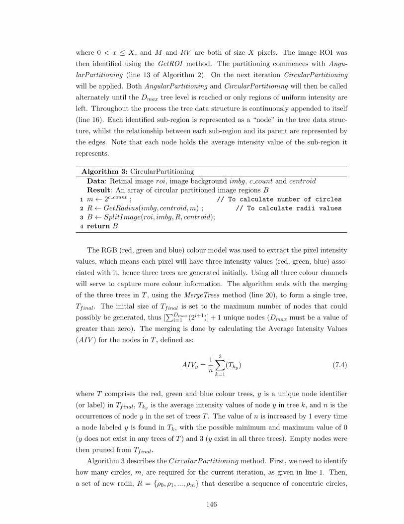
where 0 < x ≤ X, and M and RV are both of size X pixels. The image ROI was

then identified using the GetROI method. The partitioning commences with Angu-

larPartitioning (line 13 of Algorithm 2). On the next iteration CircularPartitioning

will be applied. Both AngularPartitioning and CircularPartitioning will then be called

alternately until the Dmax tree level is reached or only regions of uniform intensity are

left. Throughout the process the tree data structure is continuously appended to itself

(line 16). Each identified sub-region is represented as a “node” in the tree data struc-

ture, whilst the relationship between each sub-region and its parent are represented by

the edges. Note that each node holds the average intensity value of the sub-region it

represents.

Algorithm 3: CircularPartitioning

Data: Retinal image roi, image background imbg, c count and centroidResult: An array of circular partitioned image regions B

1 m← 2c count ; // To calculate number of circles

2 R← GetRadius(imbg, centroid,m) ; // To calculate radii values

3 B ← SplitImage(roi, imbg,R, centroid);4 return B

The RGB (red, green and blue) colour model was used to extract the pixel intensity

values, which means each pixel will have three intensity values (red, green, blue) asso-

ciated with it, hence three trees are generated initially. Using all three colour channels

will serve to capture more colour information. The algorithm ends with the merging

of the three trees in T , using the MergeTrees method (line 20), to form a single tree,

Tfinal. The initial size of Tfinal is set to the maximum number of nodes that could

possibly be generated, thus [∑Dmax

i=1 (2i+1)] + 1 unique nodes (Dmax must be a value of

greater than zero). The merging is done by calculating the Average Intensity Values

(AIV ) for the nodes in T , defined as:

AIVy =1

n

3∑k=1

(Tky) (7.4)

where T comprises the red, green and blue colour trees, y is a unique node identifier

(or label) in Tfinal, Tky is the average intensity values of node y in tree k, and n is the

occurrences of node y in the set of trees T . The value of n is increased by 1 every time

a node labeled y is found in Tk, with the possible minimum and maximum value of 0

(y does not exist in any trees of T ) and 3 (y exist in all three trees). Empty nodes were

then pruned from Tfinal.

Algorithm 3 describes the CircularPartitioning method. First, we need to identify

how many circles, m, are required for the current iteration, as given in line 1. Then,

a set of new radii, R = {ρ0, ρ1, ..., ρm} that describe a sequence of concentric circles,

146

is calculated using the GetRadius method. A set of new additional nodes, B, are then

generated (if necessary) using the SplitImage method (line 3) and returned. Note that a

“termination criterion” is used in the SplitImage method to determine if nodes splitting

is required. Details of the termination criterion used in this chapter are presented in

Sub-section 7.2.1.

The AngularPartitioning method, described in Algorithm 4, begins by identifying

the number of radii (m) that are required (line 1). The radii define the angular parti-

tions which in turn are presented in terms of a set of circular arcs A = {α0, α1, . . . , αm}.Each arc α is defined by an angle θ = 2π/m, used in the GetTheta method (line 2).

As in the case of the CircularPartitioning algorithm, the SplitImage method is called

to decompose the image, as indicated, to produce an appropriate set of nodes B.

Algorithm 4: AngularPartitioning

Data: Retinal image roi, image background imbg, a count and centroidResult: An array of angular partitioned image regions B

1 m← 2× 2a count ; // To calculate number of angular lines

2 θ ← GetTheta(m) ; // To calculate the angle between angular lines

3 B ← SplitImage(roi, imbg,m, θ, centroid);4 return B

7.2.1 Termination Criterion

As noted in the above, the nature of the termination criterion is important in any image

decomposition technique. For the work described here a similar termination criterion

as described in [72] was adopted. However, colour intensity values were considered

instead of energy (extracted from the image texture information) due to the difficulties

in identifying drusen. Therefore, the homogeneity of a parent region, ω, was defined

according to how well a parent region represents its child regions’ intensity values. If

the intensity value, which is derived from the average intensity values of all pixels in a

particular region, of a parent is similar (less than a predefined homogeneity threshold,

τ) to all of its child regions, the parent region is regarded as being homogeneous and is

not decomposed further. Otherwise, it will be further partitioned. Calculation of the

ω value for a child region i of a parent region p can be formalised as:

ωi =|(µp − µi)|

µp(7.5)

where µp is the average intensity value for the parent region and µi is the average

intensity value for child region i. Note that a lower τ value will make the decomposition

process more sensitive to colour intensity variations in the image, and will produce a

larger tree as more nodes will be kept (but it is limited to the maximum number of

147

nodes that can be produced by a predefined tree’s maximum level of depth, Dmax).

The decomposition process is performed iteratively until it has reached the Dmax value

or all sub-regions are homogeneous.

7.3 Feature Exraction

In this section the application of a graph mining technique, employed to extract the im-

age features from the trees generated by the image decomposition process, is described.

The generated tree (representing an image) was conceptualised as a labelled graph (see

Chapter 3, Sub-section 3.5.3), thus T = {V,E, LV , LE , φ}, where LV and LE are sets

of labels for the nodes and edges in T respectively, while φ defines the label mapping

function [107]. With respect to the image representation described in this section, a set

LV of three node labels was defined as LV = {equal, high, low}. A node label is deter-

mined by computing the difference between itself and its parent. Edges on the other

hand was labelled according to the relative spatial relationship between the parent and

child nodes connected by each edge, LE = {nw, sw, ne, se, inner, outer}. The aim of

the feature extraction process, in the context of this chapter, was to identify frequent

sub-graphs (the definition of a sub-graph was given in Chapter 3, Sub-section 3.5.3).

This was achieved using a Weighted Frequent Sub-graph Mining (WFSM) algorithm.

Sub-section 7.3.1 provides an overview of the gSpan Frequent Sub-graph Mining (FSM)

algorithm, on which the proposed WFSM algorithm is founded. The proposed WFSM

algorithm, that considers both node and edge weights to identify frequent sub-trees, is

described in Sub-section 7.3.2.

7.3.1 Frequent Sub-graph Mining

As stated in Chapter 3 (see Sub-section 3.5.3.1), FSM is concerned with the discovery

of frequent (interesting) sub-graphs. A sub-graph, g, is interesting if it support (occur-

rence count), sup(g), in a graph dataset is greater than a predefined support threshold,

σ (0 < σ ≤ 1). Given a graph dataset, D, the support of a sub-graph g in dataset D is

formalised as:

supD(g) =freqD(g)

|D|(7.6)

freqD(g) = |{Gi ∈ D|g ⊆ Gi}| (7.7)

where |.| is the cardinality of a set and sub-graph g is a portion of one or more of

the graphs contained in D. A sub-graph g is frequent if and only if sup(g) ≥ σ. The

FSM problem is directed at finding all frequent sub-graphs in D. There are a number

of different FSM algorithms that can be found in the literature. With respect to the

148

work described in this chapter, the popular gSpan [208] FSM algorithm was used as the

foundation for the proposed WFSM algorithm. Before describing the WFSM algorithm

the gSpan algorithm will be considered first. The gSpan algorithm, as proposed in [208],

is presented in Algorithm 5.

Algorithm 5: gSpan(D, σ)

Data: D = a graph dataset, σ = minimum support thresholdResult: F = frequent sub-graphs

1 Sort the labels of nodes and edges in D by their frequency;2 Remove infrequent nodes and edges;3 Relabel the remaining nodes and edges;4 F1 ← all frequent 1-edge graphs in D;5 Sort F1 in DFS lexicographic order;6 F ← F1;7 for ∀e ∈ F1 do8 c← e;9 subGraphMining(c, σ,D,F);

10 D ← D − c;11 if |D| < σ then12 break;13 end

14 end

Line 1 to 3 in Algorithm 5 performed a number of preliminary tasks required be-

fore the identification of frequent sub-graphs can commence. These preliminary tasks

include the removal of all the infrequent labels and edges, and relabeling the remain-

ing ones. Then, the seeds (1-edge graphs) that will be used to generate candidate

sub-graphs are identified in line 4. Once these are identified, the subsequent task is

to identify the frequent sub-graphs by determining the support of the candidate sub-

graphs. This is performed by the subGraphMining procedure in line 9 (details of this

procedure are presented in the following paragraph). The searching of frequent sub-

graphs will terminate once all frequent 1-edge graphs have been processed (line 11).

Using canonical labelling and DFS lexicographic ordering, the subGraphMining pro-

cedure prunes any duplicate sub-graphs and their descendants [208]. The procedure

then recursively grows the current frequent sub-graphs, c, by one edge and decides if

further growth is necessary (line 6 to 10). Note that the right-most extension shown in

line 6 guarantees that the complete set of frequent sub-graphs is generated in DFS lex-

icographic order [208]. Although gSpan produced a competitive performance to other

algorithms, it was found that it does not operates well on large graph datasets with a

small number of labels [106]. To address this issue, WFSM was employed with respect

to the work described in this chapter.

149

Procedure subGraphMining(c, σ,D,F)

1 if c 6= min(c) then2 return;3 end4 F ← F ∪ c;5 G← �;6 Scan D once, find every edge e such that c can be right-most extended to

frequent c ∪ e; G← c ∪ e;7 Sort G in DFS lexicographic order;8 for ∀g ∈ G do9 if sup(g) ≥ σ then

10 subGraphMining(g, σ,D,F);11 end

12 end

7.3.2 Weighted Frequent Sub-graph Mining

The idea behind the proposed WFSM algorithm is the observation that some objects

in an image can generally be assumed to be more important than other objects. With

respect to the work presented in this thesis it was conjectured that, nodes that are

some “distance” away from their parent are more informative than those that are not.

In the context of the work described here, such distance is measured by considering the

difference of average colour intensity between a parent and its child nodes, normalised

to the average colour intensity of the parent, which is equivalent to equation (7.5)

above. The intuition here is that normal retinal pixels have similar colour intensity,

while a substantial difference in intensity may indicate the presence of drusen. Thus,

the quality of the information in the un-weighted tree representation can be improved

by assigning weights to nodes and edges according to this distance measure.

The specific graph weighting scheme adopted with regard to the WFSM algorithm

advocated in this chapter is based on the work described in [107]. In the context of the

proposed approach, two weights are assigned to each sub-graph g:

1. Nodes weight: Since abnormalities in retinal images (AMD and other disease)

commonly appear to be brighter than normal retina, higher value weights are

assigned to such nodes (as these nodes are deemed to be more important).

2. Edges weight: The edge weight (that defines the relationship between a child

and its parent) is defined by the distance as described above.

Given a graph dataset, D = {G1, G2, . . . , Gz}, each node of a graph contains an average

intensity value for a region within the image I it represents.

Definition 7.1. Given a graph dataset D = {G1, G2, . . . , Gz} and image set I =

{I1, I2, . . . , Iz}, a graph Gi that represents an image Ii contains a set of nodes {v1, v2,

150

. . . , vp} and edges {e1, e2, . . . , eq}. Each node vj represents a region in image Ii. The

nodes are assigned a set of values {a1, a2, . . . , ap} where each aj corresponds to the

average intensity value of vj.

A scheme to compute graph weights similar to that described in [107] was adopted

with respect to the work described in this chapter. The node (and edge) weights for g

are calculated by dividing the sum of the average node (and edge) weights in the graphs

that contain g with the sum of the average node (and edge) weights of all graphs in D.

Thus:

Definition 7.2. Given a graph dataset D = {G1, G2, . . . , Gz}, Gi becomes a weighted

graph by assigning: (i) {nw1 , nw2 , . . . , nwp} to its nodes {v1, v2, . . . , vp}, and (ii) {e1, e2,

. . . , eq} to its edges {lw1 , lw2 , . . . , lwq} respectively; the average weights associated with

Gi are then defined as:

Wavg n(Gi) =

∑pj=1 nwj

p(7.8)

Wavg e(Gi) =

∑qj=1 lwj

q(7.9)

where lwj is as defined in equation (7.5) and nwj is defined as the average intensity

value of the corresponding node. The sum of the weights within D are calculated as

follows:

Wsum n(D) =z∑i=1

Wavg n(Gi) (7.10)

Wsum e(D) =z∑i=1

Wavg e(Gi) (7.11)

Using equations (7.8), (7.9), (7.10) and (7.11), the nodes and edges weights of a

sub-graph g can be computed using equation (7.12) and (7.13) respectively.

Definition 7.3. Given a graph dataset D = {G1, G2, . . . , Gz}, and a sub-graph g, let

the set of graphs where g occurs be given by 4D(g). Then, the weights of g with respect

to D are defined as:

ND(g) =

∑Gi∈4D(g)Wavg n(Gi)

Wsum n(D)(7.12)

ED(g) =

∑Gi∈4D(g)Wavg e(Gi)

Wsum e(D)(7.13)

151

d

c s

x

d s

x

s d

c c s

x

c d

c s d

(g) (G1) (G2) (G3)

0.3

0.5 0.4

0.3

0.8

0.7 0.5

0.3 0.6

0.4

0.7

0.4

0.6

0.3 0.5

e1 e2

e3

e1 e2

e3 e4

e1 e2

e3 e4 e5

Figure 7.3: An example of calculating graph weights using the proposed weighted graphmining algorithm

It is suggested that the utilisation of node and edge weights together can reduce

the computational cost of FSM, as less frequent sub-graphs will be identified. To

extract frequent sub-trees (image features) that are useful for classification, a WFSM

algorithm, an extension of the well-known gSpan algorithm [208], was defined. The

WFSM algorithm operated in a similar manner to that described in [107], but took both

node and edge weightings into consideration (rather than node or edge weightings).

Definition 7.4. A sub-graph g is weighted frequent, with respect to D, if it satisfies

the following two conditions:

(C1)ND(g)× sup(g) ≥ σ, (C2)ED(g) ≥ λ (7.14)

where σ denotes a predefined weighted minimum support threshold and λ denotes the

weighted minimum edge threshold.

Example. Consider a graph set D = {G1, G2, G3} in Figure 7.3 where each node

consists of a label (symbol inside a node) and an average intensity value of the region

in the image it represents (a real valued number located next to it). The symbol next

to each edge indicates the edge label. The weight of each node is equivalent to the node

average intensity value. Thus, for example, the weight of the first node, node ‘x’, in

G1, nw1(G1) = 0.3 while the second node (‘d’) nw2(G1) = 0.5. Given an edge label e1

of G1, the edge weight is computed as lw1(G1) = |0.3−0.5|0.3 = 0.6667. Thus, the weights

of the other edges, with respect to each graph, are as follows:

• Graph G1 : lw2(G1) = |0.3−0.4|0.3 = 0.3333, lw3(G1) = |0.4−0.3|

0.4 = 0.25.

• Graph G2 : lw1(G2) = |0.8−0.7|0.8 = 0.125, lw2(G2) = |0.8−0.5|

0.8 = 0.375, lw3(G2) =|0.5−0.3|

0.5 = 0.4, lw4(G2) = |0.5−0.6|0.5 = 0.2.

152

• Graph G3 : lw1(G3) = |0.4−0.7|0.4 = 0.75, lw2(G2) = |0.7−0.4|

0.7 = 0.4286, lw3(G2) =|0.4−0.6|

0.4 = 0.5, lw4(G2) = |0.6−0.5|0.6 = 0.1667, lw5(G2) = |0.6−0.3|

0.6 = 0.5.

The average node and edge weights are then computed; Wavg n(G1) = 0.3+0.5+0.4+0.34 =

0.375,Wavg n(G2) = 0.8+0.7+0.5+0.3+0.65 = 0.58,Wavg n(G3) = 0.4+0.7+0.4+0.6+0.5+0.3

6 =

0.4833,Wavg e(G1) = 0.6667+0.3333+0.253 = 0.4167,Wavg e(G2) = 0.125+0.375+0.4+0.2

4 =

0.275,Wavg e(G3) = 0.75+0.4286+0.5+0.1667+0.55 = 0.4691. Thus, Wsum n(D) = 0.375 +

0.58 + 0.4833 = 1.4383,Wsum e(D) = 0.4167 + 0.275 + 0.4691 = 1.1608. Given a

sub-graph g, which occurs in G2 and G3, ND(g) = 0.58+0.48331.4383 = 0.7393, ED(g) =

0.275+0.46911.1608 = 0.641 and supD(g) = 2/3 = 0.6667.

To apply the proposed graph weighting scheme, a modification on the gSpan algo-

rithm presented above was necessary. This was done by replacing the ‘subGraphMin-

ing‘ procedure with the ‘weightedSubGM‘ procedure described below. The “weighted

minimum support” threshold, σ, and “weighted minimum edge” threshold, λ, were

introduced to replace the initial minimum support threshold (σ).

Procedure weightedSubGM(c, σ,D,F)

1 if c 6= min(c) then2 return;3 end4 if ND(c) ≥ σ ∧ ED(c) ≥ λ then5 F ← F ∪ c;6 end7 G← �;8 Scan D once, find every edge e such that c can be right-most extended to

frequent c ∪ e; G← c ∪ e;9 Sort G in DFS lexicographic order;

10 for ∀g ∈ G do11 if ND(g) ≥ σ ∧ ED(g) ≥ λ then12 weightedSubGM(g, σ,D,F);13 end

14 end

The output of the application of the weighted frequent sub-graph mining algorithm

was then a set of Weighted Frequent Sub-Trees (WFSTs). In order to allow the applica-

tion of existing classification algorithms to the identified WFSTs, feature vectors were

built from them. The approach presented in this chapter is similar to that described

in [107]. The identified set of WFSTs was first used to define a feature space. Each

image was then represented by a single feature vector comprised of some subset of the

WFSTs in the feature space. In this manner the input set can be translated into a two

dimensional binary-valued table of size z×h; of which the number of rows, z, represents

the number of images and h the number of identified WFSTs. An additional class label

column was added.

153

The number of features discovered by the WFST mining algorithm is determined

by both σ and λ values. Previous work conducted by the author, and presented in [90],

shows that relatively low σ and λ values were required in order to generate a sufficient

number of WFSTs. Setting low threshold values however results in large numbers of

WFSTs, of which many were found to be redundant and/or ineffective in terms of

the desired classification task. Thus, a feature selection process was applied to the

discovered features. This is discussed in the following section.

7.4 Feature Selection

Feature selection was conducted by means of a feature ranking strategy using a SVM

as described in Chapter 5 (see Section 5.3). The input to the feature ranking algo-

rithm was a set of identified WFSTs and a range of c values (used to identify the best

penalty parameter C), and the output was a ranked list of WFSTs sorted in descending

order according to their weights. The feature selection process was then concluded by

selecting the top K WFSTs, consequently the size of the feature space was reduced by

a factor of h−K.

7.5 Classification Technique

The final stage of the proposed tree based retinal image classification process is the

classification stage. As described above, each image was represented by a feature vector

of WFSTs. Any appropriate classification technique could then be applied. In the

context of the work described in this chapter, Naıve Bayes (NB) and SVM were used.

These techniques were selected because they are either parameterless (NB) or have

been shown to be effective (SVM), as well as for their superior performances in the

experiments presented in Chapter 6. The nature of the NB and SVM mechanisms

adapted with respect to the work described in this chapter was similar to that described

in Chapter 6.


This section presents the experimental setup for the experiments conducted to evaluate

the tree based approach proposed in this chapter, and discusses the results produced.

Details of the experimental set up are given in Sub-section 7.6.1.

Two sets of results were produced and discussed:

1. Comparison of image classification performances generated using different levels

of depth decomposition are presented and discussed in Sub-section 7.6.2.

2. Comparison of performances with and without feature selection are presented and

discussed in Sub-section 7.6.3.

154


To evaluate the tree based representation demonstrated in this chapter, it was applied

to the retinal image datasets as described in Chapter 2. The proposed approaches

were tested to solve both binary and multiclass classification problems. Recall that

the binary problem dataset, BD, consisted of AMD and normal images, while the

multiclass dataset, MD, consisted of AMD, DR and normal images. As in the case of

the evaluations reported in Chapters 5 and 6, four evaluation metrics were again used to

measure the performances of the proposed approaches on the BD dataset: sensitivity,

specificity, accuracy and AUC. Similarly with respect to the MD dataset, the same

five evaluation metrics as used previously were adopted: sensitivity to identify AMD,

sensitivity to identify other disease, specificity, accuracy and AUC. The objectives of

the conducted experiments were:

1. Identification of the most appropriate depth of decomposition param-

eter (Dmax): To analyse the effect of different Dmax values, applied using the

image decomposition technique described in Section 7.2, on the classification per-

formances. For the experiments, the Dmax value was set to 5, 6 and 7 and the

node splitting threshold, τ , was set to 1%, 2.5% and 5%.

2. Identification of the most appropriate WFST parameter (K): To analyse

the performance of the proposed tree based techniques with respect to the size of

the feature space. In the conducted experiments, the value of K was set to 50,

100, 200, 400, 1,000, 4,000, 10,000, 12,000 and 20,000. The feature selection was

applied to the WFSTs identified using Dmax = 6 and 7, as this had already been

found to produce good classification performances with respect to both classifiers

as presented in the first experiment. It was anticipated that the classification

results would be improved by using only the most significant features.

To generate the WFSTs, two support thresholds, σ and λ, were applied. For both

experiments, a range of σ values from 10% to 90% was used (incremented in steps of

10%), and a range of λ values from 20% to 80% (incremented in steps of 20%) were

used.

To find the best parameters, C and γ (C = 2c and γ = 2g), for the SVM classifier,

similar settings as described in Chapter 6 were employed. A range of c and g values

were tested; −5 ≤ c ≤ 15 and −15 ≤ g ≤ 3 with a step of 2 between intervals. This

process was repeated five times (the training and test sets were randomly generated).

With respect to the multiclass classification evaluations, a one-against-one method was

used with respect to the SVM classifier, whereby probability estimates, as proposed in

[204], was employed to determine the winner. The posterior class probability, computed

using NB algorithm, was used directly to determine the class label for the NB classifier.

155

All the reported experiments in this chapter were carried out using five sets of TCV

(see Sub-section 1.6 for details). The presented results were generated by computing

the average and standard deviation of all results produced using the different TCV

sets. The codes to decompose the images into the tree representation and the feature

extraction were designed using Matlab. The classification techniques available in Weka

were used to perform the desired image classification. All experiments were conducted

using 1.86GHz Intel(R) Core(TM)2 PC with 2 GB RAM.

7.6.2 Experiment 1: Comparison of Classification Performances usingVarious Dmax Values

The results of the experiments used to compare the performances of image classification

using different tree depth levels, Dmax, are presented in this sub-section. Figures 7.4

and 7.5 show the results obtained based on the best accuracy and AUC for each σ. The

legends used in Figure 7.4 give the values of Dmax and τ ; thus “D5T1” corresponds to

Dmax = 5 and τ = 1%. Figures 7.4(a) and (b) show the accuracies generated by the

BD dataset, while Figures 7.4(c) and (d) show the accuracies obtained using the MD

dataset. Figures 7.5(a) and (b) depict the AUC produced using BD, while Figures 7.5(c)

and (d) show the AUCs using MD. The number of WFSTs, determined by the values

of the input parameters and generated by the approach described in Sub-section 7.3.2,

ranged from between 56,421 to 58 (BD dataset) and 57,914 to 55 (MD dataset). The

specific λ values that produced the best performance for each σ are not shown in the

figure, so as to make the presentation of the results more explicit and understandable.

The corresponding λ values will be stated instead in the supporting text.

Inspection of Figure 7.4 shows that the best accuracy achieved, with respect to the

binary class classification problem, using the BD set, was 71.6% using SVM, Dmax = 6,

τ = 1%, σ = 10%, λ = 40%; the number of WFSTs was 4,829. The best accuracy

recorded using NB on the same dataset was 65.2% using Dmax = 7, τ = 1%, σ = 20%,

λ = 20% and the number of WFSTs was 16,717. Most of the best accuracies, obtained

using different experiment settings, with respect to BD, were produced using Dmax = 6

and τ = 1%. With respect to MD, again SVM produced better results than its NB

counterpart, with a best accuracy of 57.1% achieved by the former, while the latter

scored 53.8% (both were produced using Dmax = 7, τ = 1%, σ = 20%, λ = 20%;

and the number of WFSTs was 16,717). The best performing Dmax value for MD

was not identifiable, although Dmax = 6 with τ = 1% tended to produce the best

accuracies using the NB classifier. The results presented in Figure 7.4 also indicate

that higher accuracies were obtained for the binary classification problem than the

multiclass classification problem.

Inspection of the results presented in Figure 7.5 shows that the best AUC for BD

was 66.6%, obtained using NB, Dmax = 6, τ = 1%, σ = 10%, λ = 40%; the number

156

(a)

(b)

(c)

(d)

Figure 7.4: Average classification accuracy using (a) NB and BD, (b) SVM and BD, (c)NB and MD and (d) SVM and MD

157

of WFSTs was 4,829. The best AUC for SVM was 65.6%, which was achieved using

Dmax = 7, τ = 5%, σ = 10%, λ = 40%; the number of WFSTs was 31,451. Most of

the best AUCs produced by NB using other parameters setting were recorded using

Dmax = 6 and τ = 1%, while no similar evidence were found with respect to the SVM

classifier (see Figure 7.5(a) and (b)). With regards to MD dataset, again NB produced

better AUC values compared to SVM. The best was 67.9%, achieved using Dmax = 7,

τ = 1%, σ = 10%, λ = 20%; the number of WFSTs was 40,592. SVM recorded the best

AUC of 66.1% using Dmax = 7, τ = 1%, σ = 20%, λ = 20%; the number of WFSTs was

15,749. Similar to the case of the BD dataset, usage of Dmax = 6 and τ = 1% tended

to produce higher AUCs for NB using the MD dataset, as shown in Figure 7.5(c). No

clear winner (with respect to the best Dmax value) was found using the SVM classifier

(see Figure 7.5(d)).

With regards to the other evaluation metrics used, the results are as follows (these

results are not shown in both Figures 7.4 and 7.5):

• Experiments on the BD dataset produced the following results:

– The best sensitivity was 100% using SVM. Such sensitivity was achieved

using a number of different parameter settings. With respect to NB, the

best sensitivity was 88.9% achieved using Dmax = 5, τ = 1%, σ = 90%,

λ = 20%; the number of and WFSTs was 58.

– The best specificity was 61.7%, obtained using NB, Dmax = 6, τ = 1%,

σ = 30%, λ = 20%; the number of WFSTs was 1,950. SVM produced the

best specificity of 47.8% using Dmax = 7, τ = 5%, σ = 10%, λ = 40%; the

number of WFSTs was 31,451.

• Experiments on the MD dataset produced the following results:

– The best sensitivity to identify AMD was 100% using SVM, Dmax = 7,

τ = 1%, σ = 80%, λ = 20%; the number of WFSTs was 1,037. The best

sensitivity to identify AMD using NB was 79.3% (Dmax = 5, τ = 1%,

σ = 90%, λ = 20%; the number of WFSTs was 56).

– The best sensitivity to identify other disease was 65.4%, achieved using NB,

Dmax = 7, τ = 1%, σ = 10%, λ = 20%; the number of WFSTs was 40,592.

SVM produced the best sensitivity to identify other disease of 58.0% using

Dmax = 7, τ = 1%, σ = 20%, λ = 20%; the number of WFSTs was 15,749.

– The best specificity was 57.7% achieved using NB, Dmax = 5, σ = 10%,

λ = 20%; the number of WFSTs was 2,470. SVM produced a low specificity

of 39.5% using Dmax = 7, τ = 1%, σ = 10%, λ = 20%; the number of

WFSTs was 40,592.

158

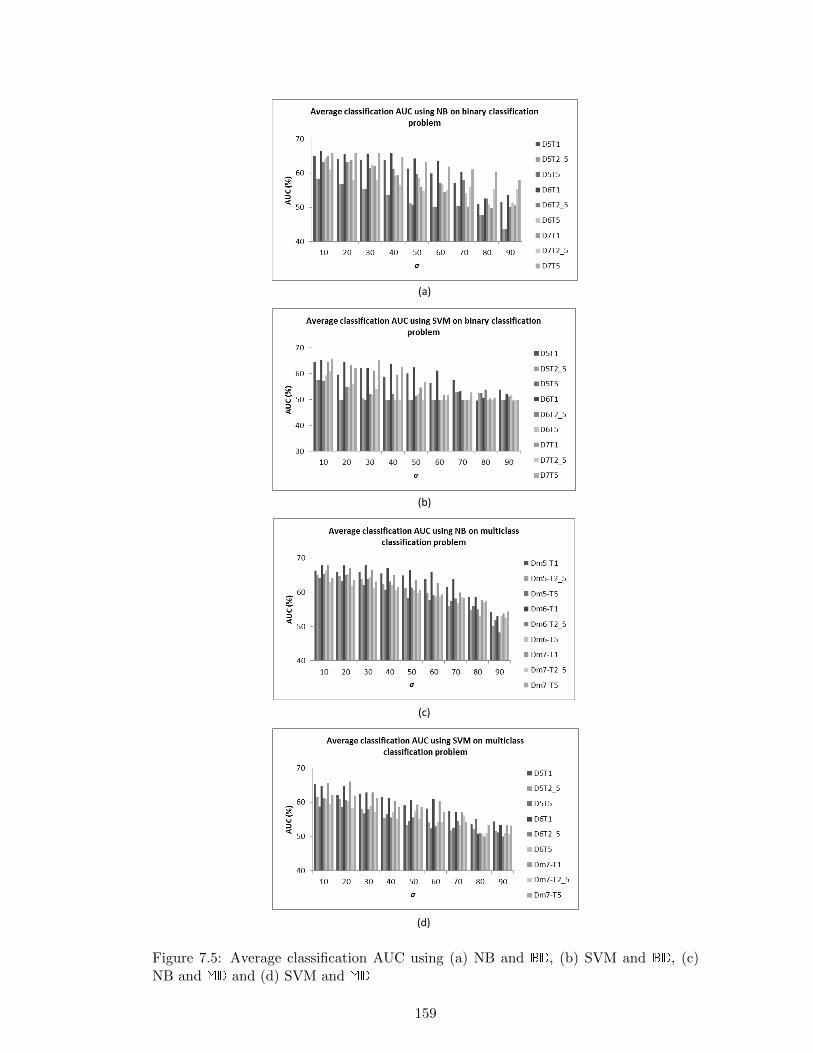
(a)

(b)

(c)

(d)

Figure 7.5: Average classification AUC using (a) NB and BD, (b) SVM and BD, (c)NB and MD and (d) SVM and MD

159

Based on the results presented in this sub-section, the main findings can be sum-

marised as follows:

1. The best classification accuracies for the BD dataset were 71.6% (SVM) and 65.2%

(NB), while the best for the MD dataset were 57.1% (SVM) and 53.8% (NB).

2. The best classification AUCs for the BD dataset were 66.6% (NB) and 65.6%

(SVM), while the MD dataset recorded 67.9% (NB) and 66.1% (SVM).

3. Most of the best results (with respect to accuracy and AUC) were produced using

Dmax = 6.

4. Most of the best accuracies and AUCs were also produced using lower σ (< 30%)

and λ (< 50%).

5. The node splitting threshold τ = 1% tended to produce the best classification

results compared to other τ values used in the experiments.

6. The proposed approach performed better on the BD dataset than the MD dataset.

7. The classification accuracy and AUC decreased when the value of σ was increased.


Both classification algorithms, NB and SVM, produced comparable results with respect

to the datasets used (greater than 60% for the BD dataset and greater than 50% for

MD). Inspection of the standard deviations for the results indicate that similar accuracy

and AUC were produced across the different sets of TCV, with an average of less than

2% for the MD dataset and less than 3% for BD (irrespective of the classifiers used

and the parameter settings). Looking back at Figures 7.4 and 7.5, the performance

of the proposed approach decreased when the σ value was increased. When higher

values of σ were used more FSTs (which may include relevant and informative FSTs)

were pruned. A similar effect was produced by λ, where most of the best results

were generated using λ < 50%. The results reported also indicated that Dmax = 6

produced better accuracies and AUCs compared to Dmax = 7. This was unexpected

as the assumption was that higher Dmax values would produce better results because

they were expected to encapsulate a greater proportion of the information in the input

images. It was conjectured that the reason for the unexpected result was that when

using a high Dmax value many irrelevant WFSTs were included in the feature space

and that this had a consequent adverse effect on classification performances. Therefore,

it was expected that the feature selection approach stated in Section 7.4 would remedy

this situation. This was evaluated in the following reported experiments. Note that the

following section presents only the results generated using Dmax = 6 and 7 as Dmax = 5

did not serve to enhance classification performances. With respect to parameter τ , the

160

reported results in this section indicate that best results were mostly produced using

τ = 1% or 5%. Thus, τ = 2.5% was not considered in the following experiments. The

σ value was limited to 50% as it had been found that larger values did not produce a

significant improvement in the classification results.

7.6.3 Experiment 2: Comparison of Different Values of K

The results of experiments presented in this sub-section compared the results produced

using various K values (the K value determined the number of WFSTs to be kept

for classification after feature selection). As stated in Sub-section 7.6.1, experiments

were conducted using different K values: 50, 100, 200, 400, 1,000, 4,000, 10,000, 12,000

and 20,000. However, only the results using K values of 50, 1,000 and 4,000 are

presented in the tables because these produced the best classification performances

with respect to both classifiers. Tables 7.1 and 7.2 show the results produced using NB

and SVM respectively when applied to the BD dataset. The results generated using

the same classifiers when applied to the MD dataset are given in Tables 7.3 and 7.4.

The first column of the tables labelled “Data”, defines the Dmax, τ and σ values used

to generate the features; thus the label “D6T1σ10” corresponds to Dmax = 6, τ = 1%

and σ = 10%. Each σ value was tested against all λ values, however in the tables only

the best performing λ value associated with each σ value (with respect to classification

accuracy) is included. The definition of other column labels in Tables 7.1 and 7.2

are as follow: (i) “Sens” represents sensitivity, (ii) “Spec” corresponds to specificity,

(iii) “Acc” represents accuracy and (iv) AUC. With regards to Tables 7.3 and 7.4, the

column labels “Sens1” and “Sens2” represent sensitivity to identify AMD and other

disease images respectively. Two values are recorded in each column (except in the

first column), corresponding to the average and standard deviation (in bracket) of the

results obtained across five sets of TCV. Note that the tables include some missing

values because the number of WFSTs for the corresponding entries were less than the

specified K value.

Inspection of Tables 7.1 and 7.2 show that high accuracies were achieved (all were

greater than 60%) using both classifiers; the best were 98.4% (Dmax = 7, τ = 1%, σ =

10% and λ = 20%) for NB, and 99.9% (Dmax = 7, τ = 5%, σ = 10% and λ = 20%) for

SVM. These were produced using K = 4, 000. The best AUCs were 99.6% (Dmax = 7,

τ = 1%, σ = 10%, λ = 20% and K = 1, 000) and 99.9% (Dmax = 7, τ = 5%, σ = 10%,

λ = 20% and K = 4, 000) for NB and SVM respectively. With respect to the results

produced when feature selection was not undertaken (presented in the foregoing sub-

section), application of feature selection produced an average improvement of more than

30% for both accuracy and AUC. These results show that feature selection significantly

improved the classification performances. Further inspection of both tables reveals that

K = 1, 000 and 4,000 produced comparable results, where the difference between the

161

best accuracies and AUCs produced using both K values, irrespective of the classifiers

used, was less than 1%. The presented results also show that the classifiers tended

to perform the best, with respect to the BD dataset, using Dmax = 7 and σ = 10%.

No evidence was obtained concerning the best λ value, although the best accuracy

and AUC were generated using λ = 20%. The results of the other evaluation metrics

produced, when applying the proposed approach to the BD dataset, were as follows:

• The best sensitivities were 99.3% (Dmax = 7, τ = 1%, σ = 10%, λ = 20% and

K = 4, 000) for NB and 100% (this was achieved using a number of different

parameter settings) for SVM.

• The best specificities were 96.9% (produced using the same parameter settings as

the best sensitivity) for NB and 100% (Dmax = 7, τ = 5%, σ = 10%, λ = 20%

and K = 4, 000) for SVM.

Observation of Tables 7.3 and 7.4 indicate that SVM performed better than NB by

producing the highest accuracy and AUC. The best accuracy and AUC produced by

SVM were 98.1% and 98.5% (both were produced using Dmax = 7, τ = 1%, σ = 10%,

λ = 40% and K = 4, 000) respectively. With respect to NB, the best accuracy and AUC

were 86.3% and 96.3% each (both were generated using Dmax = 7, τ = 1%, σ = 10%,

λ = 20% and K = 1, 000). Looking back at the results presented in the previous

sub-section, it can be observed that by selecting only the K most relevant WFSTs,

a better average performance of 38% (accuracy) and 30% (AUC) was achieved using

all WFSTs (with respect to the MD dataset). Similar to the results obtained using

the BD dataset, Dmax = 7 and σ = 10% tended to produce the best classification

performances. The results also show that τ = 1% performed batter than τ = 5%.

Further inspection on the tables reveals that λ = 20% consistently produced good

results. However, the best accuracy and AUC, with respect to the MD dataset, were

obtained using λ = 40%. Thus, it is conjectured that better classification results would

be produced using λ ≤ 40%. The performances with respect to the other evaluation

metrics considered, when the proposed approach was applied to the MD dataset, were

as follows:

• The best sensitivity to identify AMD was 88.0% (Dmax = 7, τ = 1%, σ = 10%,

λ = 20% and K = 1, 000) for NB and 100% (this occurred using several different

parameter setting combinations) for SVM.

• The best sensitivity to identify other disease was 85.7% (produced using the same

parameter settings as the best sensitivity to identify AMD) for NB and 97.1%

(Dmax = 7, τ = 1%, σ = 10%, λ = 40% and K = 4, 000) for SVM.

Based on the results presented in Tables 7.1, 7.2, 7.3 and 7.4, the main findings of

the evaluation regarding feature selection can be summarised as follows:

162

Table 7.1: Average classification results obtained using BD and NB

DataK = 50 K = 1, 000 K = 4, 000

λ Sens Spec Acc AUC λ Sens Spec Acc AUC λ Sens Spec Acc AUC

D6T1σ10 4089.4 74.8 84.0 90.9

2092.1 79.3 87.4 93.4

2079.2 67.8 75.0 77.6

(1.0) (2.2) (0.9) (0.7) (0.8) (0.6) (0.8) (0.8) (2.2) (0.7) (1.6) (0.7)

D6T1σ20 2088.0 74.8 83.2 88.0

2084.0 67.9 78.0 82.3

- - - - -(0.6) (1.4) (0.3) (0.4) (1.2) (1.5) (0.6) (1.2)

D6T1σ30 2088.4 66.8 80.4 87.0

2074.4 66.5 71.4 74.7

- - - - -(0.9) (1.6) (0.5) (1.4) (2.8) (1.1) (1.9) (1.0)

D6T1σ40 6085.4 70.2 79.8 84.3

6069.7 60.5 66.1 68.0

- - - - -(0.8) (1.2) (0.8) (0.5) (2.8) (2.3) (2.1) (1.1)

D6T1σ50 2087.5 66.8 79.8 82.0

- - - - - - - - - -(1.1) (1.0) (1.1) (1.0)

D6T5σ10 2082.3 75.6 79.6 88.5

2088.2 85.4 87.1 94.8

2075.2 66.1 71.9 78.0

(0.8) (1.8) (1.1) (0.4) (0.6) (1.4) (0.6) (0.4) (1.0) (1.8) (1.1) (1.2)

D6T5σ20 2084.1 74.1 80.3 86.0

2080.3 73.0 77.6 84.5

- - - - -(0.7) (1.1) (0.7) (1.0) (1.4) (0.9) (0.9) (1.2)

D6T5σ30 2080.8 66.9 75.6 84.0

2073.4 61.1 68.9 73.5

- - - - -(1.2) (1.6) (1.0) (0.7) (1.2) (1.3) (0.7) (1.3)

D6T5σ40 6082.8 64.5 76.0 80.5

6066.6 49.9 60.4 61.8

- - - - -(0.9) (0.7) (0.7) (0.6) (2.0) (2.0) (1.4) (1.6)

D6T5σ50 2083.0 61.2 74.8 82.5

- - - - - - - - - -(0.8) (2.1) (0.8) (0.4)

D7T1σ10 6088.6 73.7 83.2 91.0

2098.3 96.5 97.6 99.6

2099.3 96.9 98.4 99.5

(1.2) (1.3) (0.5) (0.5) (0.2) (0.8) (0.4) (0.1) (0.2) (1.2) (0.4) (0.1)

D7T1σ20 6088.6 73.7 83.2 91.0

2098.7 94.8 97.3 99.2

2095.6 84.8 91.6 95.1

(1.2) (1.3) (0.5) (0.5) (0.2) (0.9) (0.5) (0.2) (1.3) (1.7) (1.2) (1.1)

D7T1σ30 6088.6 73.7 83.2 91.0

6096.3 88.6 93.4 98.2

2087.7 69.5 80.8 85.9

(1.2) (1.3) (0.5) (0.5) (0.9) (1.1) (0.8) (0.6) (2.6) (0.2) (1.8) (1.7)

D7T1σ40 2088.3 76.3 83.9 90.8

2094.3 85.3 91.0 97.3

2075.3 53.6 67.2 70.1

(1.1) (1.1) (0.7) (0.7) (1.2) (2.1) (1.0) (0.6) (2.5) (3.5) (2.6) (2.4)

D7T1σ50 2086.5 72.0 81.2 87.7

2089.7 73.5 83.7 92.6 - - - - -

(0.6) (0.9) (0.6) (0.9) (0.6) (1.4) (0.3) (1.0)

D7T5σ10 2084.9 84.3 84.7 91.7

4093.7 93.4 93.6 98.8

2095.8 97.0 96.2 98.5

(0.7) (1.0) (0.6) (0.4) (0.5) (1.6) (0.5) (0.2) (0.6) (0.6) (0.6) (0.1)

D7T5σ20 6080.9 75.9 78.9 87.2

2093.5 92.6 93.1 98.2

2091.6 86.5 89.6 94.6

(0.8) (0.8) (0.4) (0.6) (0.9) (1.0) (0.9) (0.1) (1.0) (1.9) (1.1) (0.3)

D7T5σ30 2088.4 73.6 82.8 90.3

2090.1 84.4 87.9 96.0

2084.1 74.2 80.3 86.7

(1.4) (1.1) (1.0) (0.8) (0.5) (0.4) (0.4) (0.2) (1.7) (1.3) (1.5) (1.2)

D7T5σ40 2087.5 75.0 82.8 90.4

2085.7 82.5 84.5 92.5

2076.7 66.9 73.0 77.7

(0.9) (2.2) (1.2) (0.8) (0.7) (1.4) (1.1) (0.6) (2.7) (2.2) (2.4) (1.6)

D7T5σ50 2085.0 65.9 78.0 86.2

2087.3 75.5 82.7 89.5

2071.5 57.9 66.3 68.3

(0.6) (0.8) (0.5) (0.3) (1.8) (1.3) (1.4) (1.5) (2.4) (2.6) (2.1) (1.5)

163

Table 7.2: Average classification results obtained using BD and SVM

DataK = 50 K = 1, 000 K = 4, 000

λ Sens Spec Acc AUC λ Sens Spec Acc AUC λ Sens Spec Acc AUC

D6T1σ1080 91.1 55.7 78.0 73.4

20100.0 98.4 99.4 99.2

2097.0 78.3 90.0 87.7

(1.0) (0.9) (0.8) (0.9) (0.0) (0.5) (0.2) (0.3) (0.6) (1.9) (1.0) (1.2)

D6T1σ2080 91.1 55.7 78.0 73.4

2098.7 53.1 81.8 75.9

- - - - -(1.0) (0.9) (0.8) (0.9) (0.5) (1.4) (0.7) (0.9)

D6T1σ3020 94.1 55.6 79.7 74.9

2093.9 65.4 83.5 79.7

- - - - -(1.2) (1.8) (1.1) (1.3) (0.9) (0.9) (0.3) (0.4)

D6T1σ4020 93.2 58.2 80.3 75.7

6089.1 44.4 72.6 66.7

- - - - -(0.8) (1.7) (0.9) (1.0) (1.9) (1.4) (1.7) (1.5)

D6T1σ5080 91.1 55.7 78.0 73.4

- - - - - - - - - -(1.0) (0.9) (0.8) (0.9)

D6T5σ1060 92.4 50.8 76.9 71.6

2099.0 92.9 96.7 96.0

2094.2 79.2 88.6 86.7

(1.6) (1.2) (1.1) (1.0) (0.5) (2.8) (0.8) (1.2) (1.2) (2.9) (1.4) (1.8)

D6T5σ2060 92.4 50.8 76.9 71.6

2096.2 86.3 92.5 91.2

- - - - -(1.6) (1.2) (1.1) (1.0) (0.6) (2.2) (1.0) (1.3)

D6T5σ3060 92.4 50.8 76.9 71.6

6095.0 19.0 66.7 57.0

- - - - -(1.6) (1.2) (1.1) (1.0) (0.6) (1.6) (0.7) (0.8)

D6T5σ4020 100.0 0.0 62.8 50.0

20100.0 0.0 62.8 50.0

- - - - -(0.0) (0.0) (0.0) (0.0) (0.0) (0.0) (0.0) (0.0)

D6T5σ5020 100.0 0.0 62.8 50.0

- - - - - - - - - -(0.0) (0.0) (0.0) (0.0)

D7T1σ1060 99.9 20.5 70.3 60.2

60100.0 98.4 99.4 99.2

4099.5 97.3 98.7 98.4

(0.2) (1.8) (0.6) (0.9) (0.0) (0.9) (0.3) (0.4) (0.2) (0.8) (0.4) (0.5)

D7T1σ2060 99.9 20.5 70.3 60.2

60100.0 98.4 99.4 99.2

2099.5 82.9 93.3 91.2

(0.2) (1.8) (0.6) (0.9) (0.0) (0.9) (0.3) (0.4) (0.2) (1.9) (0.7) (1.0)

D7T1σ3060 99.9 20.5 70.3 60.2

60100.0 98.4 99.4 99.2

2098.5 87.5 94.4 93.0

(0.2) (1.8) (0.6) (0.9) (0.0) (0.9) (0.3) (0.4) (0.3) (2.4) (0.8) (1.1)

D7T1σ4080 96.5 21.2 68.4 58.9

2099.8 99.4 99.6 99.6

2090.0 56.8 77.6 73.4

(0.4) (1.9) (0.9) (1.1) (0.3) (0.5) (0.2) (0.3) (0.9) (3.8) (1.7) (2.2)

D7T1σ5080 96.5 21.2 68.4 58.9

2098.4 83.9 93.1 91.2

- - - - -(0.4) (1.9) (0.9) (1.1) (0.5) (1.1) (0.6) (0.7)

D7T5σ1080 95.7 35.0 73.0 65.4

6099.8 98.6 99.3 99.2

2099.9 100.0 99.9 99.9

(0.8) (2.5) (1.2) (1.5) (0.3) (0.5) (0.2) (0.2) (0.2) (0.0) (0.1) (0.1)

D7T5σ2080 95.7 35.0 73.0 65.4

6099.8 98.6 99.3 99.2

2099.8 85.1 94.2 92.4

(0.8) (2.5) (1.2) (1.5) (0.3) (0.5) (0.2) (0.2) (0.3) (3.1) (1.1) (1.5)

D7T5σ3080 95.7 35.0 73.0 65.4

6099.8 98.6 99.3 99.2

2099.2 92.6 96.7 95.9

(0.8) (2.5) (1.2) (1.5) (0.3) (0.5) (0.2) (0.2) (0.3) (1.5) (0.6) (0.8)

D7T5σ4080 95.7 35.0 73.0 65.4

2099.6 98.0 99.0 98.8

2094.5 70.8 85.5 82.6

(0.8) (2.5) (1.2) (1.5) (0.3) (1.3) (0.5) (0.7) (0.7) (0.7) (0.5) (0.5)

D7T5σ5080 95.7 35.0 73.0 65.4

2099.3 86.1 94.2 92.7

2092.3 32.0 69.8 62.1

(0.8) (2.5) (1.2) (1.5) (0.3) (2.5) (1.0) (1.3) (1.3) (1.8) (1.3) (1.4)

164

Table 7.3: Average classification results obtained using MD and NB

DataK = 50 K = 1, 000 K = 4, 000

λ Sens1 Sens2 Spec Acc AUC λ Sens1 Sens2 Spec Acc AUC λ Sens1 Sens2 Spec Acc AUC

D6T1σ10 2063.4 69.4 56.7 63.9 81.6

2063.9 72.5 65.6 67.2 81.9

2046.4 67.3 62.2 57.3 72.9

(1.5) (0.9) (2.1) (0.5) (0.2) (0.7) (0.5) (0.9) (0.4) (0.2) (1.9) (0.9) (0.9) (0.9) (0.2)

D6T1σ20 2064.9 67.8 48.2 61.8 79.4

2055.5 65.1 58.9 59.5 75.2

- - - - - -(0.7) (1.2) (1.4) (0.7) (0.5) (1.4) (0.5) (0.7) (0.5) (0.2)

D6T1σ30 2068.1 67.0 49.5 63.1 79.0

2050.2 61.9 58.5 56.2 71.4

- - - - - -(0.4) (1.1) (0.7) (0.4) (0.5) (2.5) (0.7) (1.8) (1.5) (0.2)

D6T1σ40 2061.2 65.8 57.2 61.8 77.4

6048.9 58.2 52.6 52.9 67.6

- - - - - -(1.3) (0.6) (1.7) (0.7) (0.2) (1.2) (1.2) (1.6) (0.4) (0.2)

D6T1σ50 2059.5 57.3 48.9 56.2 72.6

- - - - - - - - - - - -(1.1) (1.5) (1.4) (1.1) (0.8)

D6T5σ10 4067.7 65.6 50.0 62.6 79.7

2065.8 70.5 63.8 66.8 84.0

2049.4 61.4 55.8 55.0 72.6

(1.6) (1.3) (1.7) (1.0) (0.6) (1.6) (2.2) (2.1) (0.5) (0.5) (0.8) (0.6) (1.9) (0.7) (0.5)

D6T5σ20 2069.2 57.5 53.6 61.4 77.6

2051.3 61.6 57.7 56.4 75.0

- - - - - -(0.5) (1.5) (1.0) (0.4) (0.4) (1.5) (1.6) (3.1) (0.6) (0.3)

D6T5σ30 2068.1 47.3 46.8 55.9 74.5

2050.5 58.2 48.8 52.7 69.6

- - - - - -(1.6) (1.9) (1.6) (0.4) (0.5) (0.9) (0.8) (1.4) (0.7) (0.6)

D6T5σ40 2065.1 49.3 49.1 55.9 70.9

2047.0 49.7 39.3 46.0 63.4

- - - - - -(0.7) (1.4) (3.3) (1.3) (0.2) (2.5) (1.0) (1.8) (0.9) (0.8)

D6T5σ50 2058.8 54.7 47.4 54.6 73.0

- - - - - - - - - - - -(0.9) (1.6) (2.2) (0.6) (0.4)

D7T1σ10 2072.7 72.2 54.8 68.1 83.6

2088.0 85.7 84.0 86.3 96.3

2081.6 84.4 80.5 82.3 92.4

(0.7) (0.9) (1.0) (0.5) (0.4) (1.4) (0.8) (0.5) (0.5) (0.2) (1.2) (0.7) (1.2) (0.5) (0.4)

D7T1σ20 2073.7 66.7 57.1 67.3 83.4

2079.6 79.5 77.4 79.1 91.9

2070.2 72.8 69.2 70.8 83.5

(1.2) (1.7) (1.4) (1.3) (0.5) (0.6) (0.8) (1.3) (0.6) (0.3) (1.6) (0.6) (1.3) (0.9) (0.4)

D7T1σ30 2070.8 68.9 50.9 65.2 81.4

2077.9 75.3 69.9 75.1 88.2

2059.9 65.7 57.7 61.3 76.8

(1.1) (1.1) (0.9) (0.5) (0.2) (1.4) (1.6) (1.6) (1.3) (0.4) (1.9) (1.1) (1.7) (0.4) (0.5)

D7T1σ40 2069.6 61.9 49.7 62.1 80.1

2071.1 70.2 61.8 68.5 83.4

2053.8 60.5 45.5 54.0 68.7

(1.6) (1.2) (1.1) (0.9) (0.4) (1.2) (0.9) (1.9) (0.6) (0.5) (1.6) (0.7) (2.4) (1.2) (0.7)

D7T1σ50 8064.7 68.6 44.6 61.0 77.4

2069.1 64.4 53.9 63.8 79.1

- - - - - -(1.6) (2.1) (1.9) (0.9) (0.8) (1.9) (1.1) (1.8) (1.3) (0.7)

D7T5σ10 2073.9 71.3 34.3 63.2 78.5

2085.5 84.4 78.4 83.4 94.8

2083.4 83.9 76.5 81.8 93.9

(0.8) (1.3) (1.0) (0.7) (0.4) (0.6) (1.5) (1.5) (0.5) (0.3) (0.3) (0.8) (2.1) (0.6) (0.1)

D7T5σ20 2071.8 65.8 38.1 61.3 78.4

2082.0 75.9 67.4 76.4 91.7

2073.7 68.6 62.6 69.3 85.4

(1.3) (1.0) (2.2) (0.6) (0.2) (1.6) (1.2) (1.3) (1.0) (0.2) (0.7) (1.2) (0.9) (0.3) (0.4)

D7T5σ30 6065.4 62.4 50.1 60.6 78.2

2074.8 69.6 63.8 70.4 86.4

2068.3 55.7 56.3 61.1 77.8

(0.8) (0.3) (1.0) (0.6) (0.6) (1.4) (1.3) (1.5) (1.0) (0.3) (0.8) (1.4) (2.1) (0.5) (0.3)

D7T5σ40 2066.6 62.8 46.3 60.3 78.9

2072.8 58.6 61.1 65.2 82.8

2057.7 50.3 47.0 52.6 69.8

(1.3) (0.8) (1.9) (0.7) (0.7) (1.2) (1.4) (1.0) (0.5) (0.3) (1.0) (2.9) (1.7) (1.1) (0.4)

D7T5σ50 2065.8 58.8 58.3 61.5 79.3

2068.6 57.8 52.6 61.0 77.8

2048.8 46.4 35.2 44.7 62.6

(1.1) (2.0) (1.0) (0.6) (0.6) (1.0) (1.0) (1.2) (0.6) (0.6) (1.6) (1.7) (1.8) (1.3) (0.5)

165

Table 7.4: Average classification results obtained using MD and SVM

DataK = 50 K = 1, 000 K = 4, 000

λ Sens1 Sens2 Spec Acc AUC λ Sens1 Sens2 Spec Acc AUC λ Sens1 Sens2 Spec Acc AUC

D6T1σ10 2089.2 59.0 0.0 57.0 64.1

2096.1 94.2 87.8 93.4 94.9

2088.8 78.2 67.1 79.9 84.2

(1.0) (1.6) (0.0) (0.8) (0.6) (1.1) (0.4) (0.9) (0.3) (0.2) (1.6) (1.0) (0.7) (0.8) (0.6)

D6T1σ20 8088.3 38.5 4.9 51.0 58.9

2080.7 71.3 43.6 68.4 74.5

- - - - - -(1.3) (3.1) (0.9) (1.2) (1.1) (1.0) (1.8) (1.5) (0.5) (0.4)

D6T1σ30 2089.9 42.8 0.0 51.9 59.4

2074.8 67.4 53.2 67.0 74.0

- - - - - -(0.7) (1.8) (0.0) (0.6) (0.5) (1.1) (1.2) (2.3) (0.8) (0.6)

D6T1σ40 8088.3 38.5 4.9 51.0 58.9

6067.3 49.0 32.9 52.7 62.3

- - - - - -(1.3) (3.1) (0.9) (1.2) (1.1) (2.0) (1.3) (1.9) (0.9) (0.7)

D6T1σ50 8088.3 38.5 4.9 51.0 58.9

- - - - - - - - - - - -(1.3) (3.1) (0.9) (1.2) (1.1)

D6T5σ10 20100.0 0.0 0.0 41.9 50.0

4090.9 67.1 20.1 65.3 71.2

2083.7 58.2 4.5 55.5 63.2

(0.0) (0.0) (0.0) (0.0) (0.0) (0.8) (1.4) (1.9) (1.1) (0.8) (0.8) (1.2) (0.8) (0.8) (0.6)

D6T5σ20 2098.9 8.5 0.0 44.2 52.2

2085.4 81.5 63.9 78.7 83.3

- - - - - -(0.4) (1.2) (0.0) (0.5) (0.4) (1.6) (1.7) (2.8) (1.2) (0.9)

D6T5σ30 20100.0 0.0 0.0 41.9 50.0

2086.8 45.7 2.2 52.1 60.1

- - - - - -(0.0) (0.0) (0.0) (0.0) (0.0) (0.4) (2.2) (0.8) (0.8) (0.6)

D6T5σ40 2067.3 49.0 43.4 55.2 64.6

2073.8 44.5 13.6 49.1 58.9

- - - - - -(2.1) (2.2) (1.5) (0.8) (0.6) (1.1) (1.6) (1.5) (0.4) (0.3)

D6T5σ50 20100.0 0.6 0.0 42.1 50.2

- - - - - - - - - - - -(0.0) (0.3) (0.0) (0.1) (0.1)

D7T1σ10 20100.0 0.0 0.0 41.9 50.0

4097.8 91.9 84.3 92.5 94.2

4099.5 97.1 96.8 98.1 98.5

(0.0) (0.0) (0.0) (0.0) (0.0) (0.8) (0.6) (1.0) (0.5) (0.4) (0.5) (0.3) (0.7) (0.3) (0.2)

D7T1σ20 20100.0 0.0 0.0 41.9 50.0

6092.9 78.4 15.3 68.8 73.9

2090.5 84.9 38.0 75.7 80.0

(0.0) (0.0) (0.0) (0.0) (0.0) (0.7) (1.5) (1.9) (0.3) (0.3) (0.9) (0.4) (2.1) (0.6) (0.5)

D7T1σ30 20100.0 0.0 0.0 41.9 50.0

2094.5 85.9 34.3 76.7 80.8

2087.2 74.6 52.6 74.4 79.6

(0.0) (0.0) (0.0) (0.0) (0.0) (0.6) (1.7) (1.2) (0.6) (0.4) (0.6) (2.1) (1.6) (0.7) (0.6)

D7T1σ40 2096.4 25.3 0.0 48.7 56.4

2095.3 94.5 86.6 92.8 94.3

2070.8 60.1 40.9 59.9 68.6

(0.6) (1.5) (0.0) (0.5) (0.4) (0.4) (0.6) (2.7) (0.4) (0.4) (2.1) (2.7) (0.8) (1.4) (1.0)

D7T1σ50 20100.0 0.0 0.0 41.9 50.0

8085.1 61.2 9.5 58.4 65.6

- - - - - -(0.0) (0.0) (0.0) (0.0) (0.0) (0.9) (1.1) (0.7) (0.6) (0.5)

D7T5σ10 20100.0 0.0 0.0 41.9 50.0

8099.8 3.8 0.0 43.0 51.0

6094.1 40.0 1.8 53.1 60.6

(0.0) (0.0) (0.0) (0.0) (0.0) (0.3) (0.9) (0.0) (0.4) (0.3) (0.7) (1.8) (0.4) (0.6) (0.5)

D7T5σ20 20100.0 0.0 0.0 41.9 50.0

20100.0 12.8 0.0 46.1 53.7

2095.0 77.8 31.1 73.4 77.9

(0.0) (0.0) (0.0) (0.0) (0.0) (0.0) (1.3) (0.0) (0.4) (0.4) (0.5) (1.7) (1.6) (0.5) (0.4)

D7T5σ30 2095.1 42.0 0.0 53.8 60.8

2093.9 90.7 84.4 90.5 92.5

2093.3 88.2 71.2 86.1 89.1

(0.9) (2.1) (0.0) (1.0) (0.8) (0.4) (1.8) (1.3) (0.6) (0.5) (0.9) (1.1) (1.1) (0.8) (0.6)

D7T5σ40 20100.0 0.0 0.0 41.9 50.0

2093.3 66.0 33.9 69.4 74.8

2081.8 60.5 41.9 64.8 71.8

(0.0) (0.0) (0.0) (0.0) (0.0) (0.5) (1.5) (1.7) (0.7) (0.6) (0.9) (1.8) (1.8) (1.3) (1.0)

D7T5σ50 20100.0 0.0 0.0 41.9 50.0

2096.3 31.2 1.0 50.9 58.4

2079.5 42.1 13.5 50.6 59.7

(0.0) (0.0) (0.0) (0.0) (0.0) (0.6) (1.0) (0.6) (0.5) (0.4) (1.0) (1.6) (1.9) (0.8) (0.6)

166

1. The best classification accuracies for the BD dataset were 99.9% (SVM) and 98.4%


2. The best classification AUCs for the BD dataset were 99.9% (SVM) and 99.6%


3. Dmax = 7 produced better results than Dmax = 6.

4. All best results were obtained using σ = 10% and λ ≤ 40%.

5. Comparable classification performances were produced for both the BD and MD

datasets, where the best accuracy and AUC for both datasets were greater than

85%.

6. Better and comparable results were produced using K = 1, 000 and 4,000.

7. Overall, the application of feature selection produced a better performance than

when feature selection was not used (as presented in the foregoing sub-section).


The results presented in the foregoing sub-section show that the proposed tree based

approach produced good classification performances, where the best accuracy and AUC

were greater than 98% (SVM) and greater than 85% (NB) with respect to both the

binary and multiclass classification problems. Inspection on the tables also revealed

that similar results were produced across different sets of TCV, with an average stan-

dard deviation of less than 2% for both datasets and classifiers. It is conclusive that

the best results were generated using Dmax = 7 and σ = 10%, more image information

will be represented by a “deeper” tree. Coupled with an appropriate feature selection

technique, better classification performances can be produced. This was manifested by

the results presented in this sub-section and in Sub-section 7.6.2, where the classifi-

cation performances produced using Dmax = 7 was significantly improved upon after

feature selection was applied. The best λ value was however not identifiable. With

regards to the number of WFSTs, K = 1, 000 and 4,000 were comparable in producing

high accuracy and AUC. It is however suggested that a lower K value is more desirable

as it entails a lower computational cost. Overall, the utilisation of feature selection

significantly improved the classification performances.

7.7 Summary

In this chapter, an approach to classifying retinal images using a tree based image rep-

resentation, coupled with a weighted graph mining technique has been described. The

approach commences with the decomposition of the images into a tree representation

167

using a combination of circular and angular partitioning. The resulting decomposition

was represented as a tree data structure to which node and edge weightings were at-

tached. A weighted frequent sub-graph mining algorithm was then applied in order

to identify weighted frequent sub-trees. These were then used to generate a feature

space to which a feature selection strategy was applied, where the top K features were

selected. The resulting set of features was then used to represent the input image set

in term of a set of feature vectors. Two established classification techniques were em-

ployed to perform image classification, namely Naıve Bayes and SVM. The evaluation

of the proposed tree based method resulted in the following main findings:

1. A lower node splitting threshold, τ , value (for the image decomposition process)

contributed to better classification results.

2. A higher levels of tree decomposition (up to level 7 in this chapter), coupled

with lower threshold values (for feature extraction) produced better results after

feature selection.

3. Feature selection significantly improved the classification performances, where

the best suggested K value was 1,000 (with respect to the image sets used in this

thesis).

4. Both classifiers produced high and comparable results, indicated that the ex-

tracted features were appropriate for used with respect to retinal screening pro-

grammes.

The reported evaluation shows that the tree based image representation gave the best

overall performance with respect to the three mechanisms (the other two were described

in Chapter 5 and 6) considered in this thesis.

168

Chapter 8

Comparison Between DifferentApproaches

This chapter presents a comparison between the three different approaches advocated

in this thesis. Section 8.1 provides a comparison in the context of the AMD detection

application on which the work in this thesis is focused, and Section 8.2 in the context of

a statistical analysis using Analysis Of Variance (ANOVA) and Tukey testing. Section

8.3 conclude this chapter.

8.1 Comparison of the Proposed Approaches in Terms ofAMD Classification

The evaluation of the three image classification approaches, as reported in the foregoing

chapters, was conducted in the context of retinal images where a medical condition,

namely AMD, may or may not exist. This section presents an overall comparison

between these approaches in terms of this application. Note that the results provided

in the foregoing chapters were generated using different sets of parameters, classifiers

and variations of the approaches. In this section, however, only the results generated

by the best parameter settings (based on the highest classification accuracy achieved),

for each approach, are presented. Table 8.1 presents the best results obtained using the

binary class, BD, dataset, whilst the best results produced using the multiclass, MD,

dataset are given in Table 8.2.

The TS, TB and TR rows shown in Tables 8.1 and 8.2 represent the best classifica-

tion results produced by the time series, tabular and tree based approaches respectively.

The right most column shows the False Negative Rate (FNR) produced by the proposed

approaches. The best results are indicated in bold font. From Table 8.1 it can be seen

that the TB and TR approaches produced high classification performances of greater

than 85% accuracy and greater than 90% AUC. From the results, the best accuracy

and AUC were both 99.9%. The FNR value was low at 1.0%. These were obtained

using the TR approach. These are excellent results. The best sensitivity and specificity

169

Table 8.1: The best average classification performances obtained using the BD dataset

Ap. Sens Spec Acc AUC FNR

TS 74.5 60.4 69.3 73.2 25.5TB 92.3 78.7 87.3 93.2 7.7TR 99.0 100.0 99.9 99.9 1.0

Table 8.2: The best average classification performances obtained using the MD dataset

Ap. Sens-AMD Sens-other Spec Acc AUC FNR

TS 57.0 48.0 50.5 52.4 70.7 43.0TB 77.3 75.3 49.2 69.7 84.7 22.7TR 99.5 97.1 96.8 98.1 98.5 0.5

were also produced by the TR approach. TS produced the worst results.

With respect to the multiclass dataset, MD, it can be observed from Table 8.2

that all the approaches produced lower classification performances compared to the

results shown in Table 8.1 when all the performance measures are collectively taken

into consideration, with exceptions to the sensitivity to identify AMD images and FNR.

Out of the three advocated approaches, only the TR approach produced an accuracy

of greater than 90%. The best accuracy and AUC achieved using TR were 98.1% and

98.5% respectively. Although not as good as the results obtained using the BD dataset,

these are still excellent results. However, higher sensitivity and FNR of 99.5% and 0.5%

respectively were recorded. Similar to the results for the BD dataset, the TR approach

outperformed the TS and TB approaches with respect to all the evaluation metrics

used. These results indicate that using the proposed tree representation, coupled with

a weighted frequent sub-graph mining algorithm, is the most appropriate with respect

to the classification of images where the features are not easily distinguishable (at least

in the case of the retinal images used as the focus for the research described in this

thesis). The TR approach also produced the most reliable results with a low FNR value

that would avoid AMD patients mistakenly screened as being healthy.

In the context of AMD identification, as reported in the literature (Chapter 3), most

of the related work emphasised the identification of drusen with the aim of grading the

severity of AMD. Out of these, only three instances could be extended to the screening

of AMD: (i) Brandon and Hoover [23], (ii) Chaum et al. [33] and (iii) Agurto et al. [5].

Details of these approaches can be found in Chapter 3 (Section 3.8) of this thesis. A

summary of the reported analysis of these systems is as follows:

1. The reported evaluation of the work proposed by Brandon and Hoover [23] was

applied not only to AMD screening (AMD v. non-AMD), but also to grade the

detected AMD. The reported overall accuracy obtained was 90%.

170

2. The work of Chaum et al. [33] was applied in a multiclass setting. The overall

reported classification accuracy was 91.3%. In their evaluation, 48 images (12.2%

of the total images used) were classified as “unknown” and excluded from the

accuracy calculation. If this number was included as miss-classifications, the

accuracy will be lower.

3. The evaluation of the work promoted by Agurto et al. [5] reported an AUC of 84%

to identify AMD images (against normal images) that contain several pathologies,

including drusen. They also presented the results of applying their approach on

AMD images with drusen only, as a result of which the recorded AUC value was

decreased to 77%. No classification accuracy was reported.

As stated in Chapter 1 (Section 1.6), it is impossible to conduct a direct comparison

between the proposed approaches and the ones described above due to data privacy

issue. Thus, all the reported classification performances provided above were gener-

ated from different sets of retinal images. However, based on these results, it can be

suggested that the proposed approaches presented in this thesis, in particular the tree

based approach, performed better than that associated with the existing work found

in the literature.

The results presented above show the potential for automated or semi-automated

AMD screening system (no such systems are in used at present), which could:

(i) provide for the large scale early detection of AMD with respect to the global aging

population,

(ii) allow for early intervention to slow down the loss of vision process associate with

AMD, and

(iii) significantly reduces the overall resource required to conduct screening programmes

(clinician would not be required to inspect every image).

Recent evidence, gathered with respect to the screening of Diabetic Retinopathy (DR)

patients using colour fundus photographs reported in [60], has shown the success of

the semi-automated screening system used in the study in reducing vision loss (in the

context of DR). The only problem with the system was the high number of false positives

(although cost-effectiveness and a reduction in the overall workload was successfully

achieved) [60]. An advantage of the approaches proposed in this thesis is that they

produced high classification performances, using the dataset described in Chapter 2,

with respect to all the evaluation metrics used.

171

8.2 Statistical Comparison of the Proposed Approaches

The comparison with respect to AMD screening reported in the foregoing section shows

that the best classification performance was produced by the third approach, TR. In

this section, a statistical analysis is presented to demonstrate that this result is indeed

significant. With respect to the work described in this thesis, where three classification

approaches were applied on two sets of data (BD and MD), the ANOVA test, coupled

with the Tukey test [192], was employed to compare the approaches.

The statistical tests reported in this section were designed to measure if two or more

“treatments” are significantly different [170]. In a machine learning domain, statistical

tests have been adopted to compare the performances of different classifiers on a given

dataset [170]. An analysis reported in [43] shows that such statistical tests have been

increasingly applied by researchers in order to validate their classification results. The

objective of these statistical tests was to support or reject the “null” hypothesis (H0)

that there is no statistical difference between the results produced by two or more com-

parable approaches to some problem [214]. In the context of classifier comparison, the

null hypothesis corresponds to the condition where two or more classification algorithms

produced the same error rates, in other words there is no statistical difference between

them [45]. Generally, this kind of statistical test commences by applying different clas-

sification algorithms to some dataset, and obtaining the error rates produced by each

algorithm. The resulting error rates are then tested against the null hypothesis. If the

result of the test causes the null hypothesis to be rejected, the compared classifiers are

said to be significantly different. There are numerous statistical tests that are described

in the literature, such as the McNemar’s test, the paired t-test and the 5×2cv (cross

validation) t-test [43, 45]. These tests are directed at the comparison of classifiers that

are applied to a single dataset. With respect to the comparison of classifiers applied to

multiple datasets, as conducted in the work described in this thesis, appropriate meth-

ods include the Analysis of Variance (ANOVA) and the Friedman test [174, 214]. The

latter was suggested in [43] in preference over the former, however it will only perform

well when a large number of data samples (n) and classifiers (k) are used (n > 10 and

k > 5). Thus, the ANOVA test was employed with respect to the work described in

this thesis.

The ANOVA test operates in terms of the mean of the “accuracies” produced by

the different considered classifiers. If they are roughly equivalent the null hypothesis

is said to be true, thus H0 : µ1 = µ2 = . . . = µk, where µi represents the mean of the

accuracy produced by classifier i. The ANOVA test computes the between classifiers

variability, between sample variability and within classifier variability [43, 174]. The

means of the accuracies of the compared classifiers are said to be different if the between

classifiers variability is significantly larger than the within classifiers variability; thus, if

this is the case, the null hypothesis can be rejected. This is indicated by the resulting p

172

value; in the context of the work presented in this thesis, the p value corresponds to the

probability that all classifiers produced the same mean. From the literature, classifiers

were deemed to be significantly different if p ≤ 0.05 [170]. In order to identify which

classifiers actually differ, the Tukey post hoc test can be applied. A Tukey test performs

multiple pairwise classifier comparisons by calculating the differences between means

of the compared classifiers. The best performing classifier is then identified if the

computed differences are large enough.

Assuming a number of k classifiers with n samples each, the ANOVA test can be

described as follows [174, 214]:

1. Compute the total sum of squares, SST :

SST =∑

X2T −

(∑XT )2

N(8.1)

where N =∑k

i=1 ni is the total number of samples, ni is the number of samples

in classifier i,∑X2T is the sum of squared scores of all samples and

∑XT is the

sum of all scores of all samples.

2. Compute the between classifiers sum of squares, SSB, as follows:

SSB =

k∑j=1

[(∑Xj)

2

nj

]− (∑XT )2

N(8.2)

where∑Xj is the total scores of samples in classifier j.

3. Compute the within classifiers sum of squares, SSW :

SSW = SST − SSB (8.3)

4. Compute the between classifiers variance, MSB:

MSB =SSBdfB

(8.4)

where dfB = k − 1 represents the between classifiers degrees of freedom.

5. Compute the within classifiers variance, MSW :

MSW =SSWdfW

(8.5)

where dfW = N − k is the within classifiers degrees of freedom.

173

6. Compute the test statistic F -ratio as follows:

F =MSBMSW

(8.6)

7. Get the critical value for the F(α,dfB ,dfW ) from the F distribution table (see Ap-

pendix B), where α is the significance level. An α of 0.05 is commonly used to

reject or accept the null hypotheses [214]. If the identified critical value is smaller

than the computed F ratio in equation (8.6), it indicates that the probability, p,

of the classifiers producing the same mean values is less or equal to α and thus

the null hypothesis can be rejected.

If the null hypothesis is rejected, as mentioned above, the Tukey post hoc test can

be applied to identify the Critical Difference (CD) between pairs of classifiers as follows:

CD = q(k,dfW )

√MSWn

(8.7)

where the value of q(k,dfW ) can be identified from the Studentised Range Distribution

[214] (see Appendix A). If the difference of the means of the compared classifiers is

greater than the identified CD value, it can be concluded that the compared classifiers

are significantly different.

In this chapter, the ANOVA test was used to compare the classification perfor-

mances of the proposed approaches. As stated in Chapter 1, the evaluation of the

proposed approaches was conducted using Ten Cross Validation (TCV). The TCV was

repeated five times; the training and test images for each TCV were randomised. The

generated accuracy for each run of the cross validation was taken as a sample for the

statistical tests described here. Thus, the number of samples used, n, was 10× 5 = 50

for each classifier. Tables 8.3 and 8.4 show the accuracies generated by each run with

respect to the BD and MD datasets respectively.

With respect to Table 8.3, the total sum of squares, SST , the between approaches

sum of squares, SSB, and the within approaches sum of squares, SSW , with respect to

the BD dataset were computed as follows:

SST = (243, 357.3975 + 383, 869.6413 + 499, 292.96)− (3,463.1+4,364.2+4,996.4)2

50+50+50

= 30, 198.73

SSB = (3,463.12

50 + 4,364.22

50 + 4996.42

50 )− (3,463.1+4,364.2+4,996.4)2

150= 23, 751.6

SSW = 30, 198.73− 23, 751.6= 6, 447.131

174

Table 8.3: Data for statistical testing generated from the BD dataset

ApproachesTS TB TR

X1 X21 X2 X2

2 X3 X23

75.0 5625 78.6 6173.469388 100.0 1000055.6 3086.9136 85.2 7256.515775 100.0 1000074.1 5486.3649 92.6 8573.388203 100.0 1000077.8 6049.7284 92.6 8573.388203 100.0 1000073.1 5340.6864 96.2 9245.56213 100.0 1000073.1 5340.6864 80.8 6523.668639 100.0 1000065.4 4274.5444 73.1 5340.236686 100.0 1000073.1 5340.6864 92.3 8520.710059 100.0 1000048.0 2304 96.0 9216 100.0 1000072.0 5184 88.0 7744 100.0 1000071.4 5102.2449 82.1 6747.44898 96.4 9292.9677.8 6049.7284 96.3 9272.97668 100.0 1000055.6 3086.9136 96.3 9272.97668 100.0 1000066.7 4444.8889 92.6 8573.388203 100.0 1000069.2 4792.7929 69.2 4792.899408 100.0 1000065.4 4274.5444 80.8 6523.668639 100.0 1000065.4 4274.5444 84.6 7159.763314 100.0 1000073.1 5340.6864 92.3 8520.710059 100.0 1000076.0 5776 92.0 8464 100.0 1000072.0 5184 80.0 6400 100.0 1000071.4 5102.2449 89.3 7971.938776 100.0 1000063.0 3963.9616 81.5 6639.231824 100.0 1000059.3 3511.7476 85.2 7256.515775 100.0 1000066.7 4444.8889 81.5 6639.231824 100.0 1000073.1 5340.6864 88.5 7825.443787 100.0 1000076.9 5916.6864 88.5 7825.443787 100.0 1000061.5 3787.1716 88.5 7825.443787 100.0 1000096.2 9244.8225 88.5 7825.443787 100.0 1000064.0 4096 92.0 8464 100.0 1000068.0 4624 84.0 7056 100.0 1000071.4 5102.2449 82.1 6747.44898 100.0 1000063.0 3963.9616 92.6 8573.388203 100.0 1000066.7 4444.8889 100.0 10000 100.0 1000066.7 4444.8889 92.6 8573.388203 100.0 1000057.7 3328.1361 88.5 7825.443787 100.0 1000073.1 5340.6864 76.9 5917.159763 100.0 1000080.8 6523.7929 84.6 7159.763314 100.0 1000073.1 5340.6864 100.0 10000 100.0 1000072.0 5184 92.0 8464 100.0 1000072.0 5184 76.0 5776 100.0 1000075.0 5625 100.0 10000 100.0 1000059.3 3511.7476 63.0 3964.334705 100.0 1000070.4 4951.9369 92.6 8573.388203 100.0 1000081.5 6638.9904 88.9 7901.234568 100.0 1000069.2 4792.7929 84.6 7159.763314 100.0 1000050.0 2500 88.5 7825.443787 100.0 1000080.8 6523.7929 92.3 8520.710059 100.0 1000073.1 5340.6864 92.3 8520.710059 100.0 1000068.0 4624 88.0 7744 100.0 1000060.0 3600 80.0 6400 100.0 10000∑

Xi 3463.1 4364.2 4996.4∑X2i 243357.3975 383869.6413 499292.96

Xi 69.3 87.3 99.9

175

The degree of freedom for SSB was dfB = 3 − 1 = 2, while the degree of freedom for

SSW was dfW = 150 − 3 = 147. The between and within approaches variance were

then computed, MSB = 23,751.62 = 11, 875.8 and MSW = 6,447.131

147 = 43.858. Finally,

F = 11,875.843.858 = 270.778 was computed. The computed F value was tested against

the critical value of F with α = 0.005 (see Appendix B). Since the critical value for

dfW = 147 is not available in the distribution table, the closest dfW was used instead,

which was dfW = 120. Therefore, the critical value for this test F(0.005,2,147) ≈ 5.54.

Since the test value of F = 270.778 was greater than 5.54, the null hypothesis was

thus rejected at p < 0.005 with respect to the BD dataset. Note that Xi in the table

represents the mean of all samples in approach i.

The summary for the ANOVA test on the MD dataset is given in Table 8.5. From

the table, the F value was F = MSBMSW

= 658.313. Since the critical value for F(0.005,2,147)

(see Appendix B) was less than 5.54, the null hypothesis was also rejected at p < 0.005

for the MD dataset.

To identify which approaches performed differently, the CD value was identified

using the Tukey test. The value of q(3, 147), taken at α = 0.05 from the Studentised

range statistic table in Appendix A was 3.31. The CD value for the BD dataset was

thus CDBD = 3.31√

43.85850 = 3.1. The value of CD for MD dataset was CDMD =

3.31√

34.68350 = 2.7568. Summaries of the results produced using the Tukey test when

applied to the BD and MD datasets are presented in Tables 8.6 and 8.7 respectively.

From the tables, the differences between the approaches were all greater than the

computed CDBD and CDMD values. Thus, it can be concluded that the difference

between the approaches, for both datasets BD and MD, is statistically significant.

8.3 Summary

In this chapter, comparisons between the proposed approaches were reported with re-

spect to the classification performances and statistical differences. The third approach,

TR, produced the best classification performances (with regard to the classification

accuracy) while the TS approach performed the worst for both datasets BD and MD.

The differences between the proposed approaches, according to the ANOVA test, were

highly significant such that the null hypothesis was rejected at p < 0.005 for both

datasets. The TR approach performed the best compared to the other two approaches

according to the conducted Tukey test, where greater difference was recorded when

these approaches were applied to the MD dataset. The TB approach performed better

than the TS approach, where the difference between these two approaches were higher

when applied to the BD dataset. Thus, in conclusion, the conducted comparisons clearly

demonstrated that the proposed TR approach outperformed the other two approaches

(at least in the context of the AMD application considered in this thesis).

176

Table 8.4: Data for statistical testing generated from the MD dataset

ApproachesTS TB TR

X1 X21 X2 X2

2 X3 X23

55.0 3025 75.0 5625 100.0 1000042.5 1806.25 75.0 5625 87.5 7656.2557.5 3306.25 75.0 5625 95.0 902552.5 2756.25 75.0 5625 90.0 810064.1 4108.81 74.4 5529.257068 94.9 9000.65746248.7 2373.6384 61.5 3786.982249 100.0 1000041.0 1683.4609 64.1 4109.138725 87.2 7600.26298543.6 1900.0881 76.9 5917.159763 94.9 9000.65746256.4 3182.0881 71.8 5154.503616 100.0 1000043.6 1900.0881 51.3 2629.848784 92.3 8520.71005962.5 3906.25 72.5 5256.25 97.5 9506.2552.5 2756.25 72.5 5256.25 97.5 9506.2545.0 2025 75.0 5625 95.0 902567.5 4556.25 72.5 5256.25 97.5 9506.2566.7 4444.448889 61.5 3786.982249 94.9 9000.65746248.7 2373.43378 66.7 4444.444444 100.0 1000046.2 2130.173254 71.8 5154.503616 94.9 9000.65746248.7 2373.43378 64.1 4109.138725 92.3 8520.71005941.0 1683.099855 64.1 4109.138725 87.2 7600.26298548.7 2373.43378 56.4 3182.117028 92.3 8520.71005950.0 2500 60.0 3600 97.5 9506.2562.5 3906.25 75.0 5625 97.5 9506.2552.5 2756.25 70.0 4900 90.0 810057.5 3306.25 67.5 4556.25 92.5 8556.2551.3 2629.85378 64.1 4109.138725 94.9 9000.65746253.8 2899.413254 64.1 4109.138725 92.3 8520.71005941.0 1683.099855 74.4 5529.257068 92.3 8520.71005951.3 2629.85378 71.8 5154.503616 94.9 9000.65746251.3 2629.85378 69.2 4792.899408 97.4 9493.75410953.8 2899.413254 71.8 5154.503616 94.9 9000.65746252.5 2756.25 77.5 6006.25 97.5 9506.2555.0 3025 77.5 6006.25 97.5 9506.2565.0 4225 67.5 4556.25 100.0 1000045.0 2025 70.0 4900 87.5 7656.2546.2 2130.173254 74.4 5529.257068 94.9 9000.65746259.0 3477.979855 66.7 4444.444444 97.4 9493.75410948.7 2373.43378 69.2 4792.899408 97.4 9493.75410951.3 2629.85378 61.5 3786.982249 92.3 8520.71005943.6 1900.061946 69.2 4792.899408 100.0 1000048.7 2373.43378 79.5 6318.211703 92.3 8520.71005960.0 3600 72.5 5256.25 95.0 902552.5 2756.25 67.5 4556.25 90.0 810065.0 4225 72.5 5256.25 92.5 8556.2560.0 3600 80.0 6400 95.0 902551.3 2629.85378 74.4 5529.257068 97.4 9493.75410946.2 2130.173254 66.7 4444.444444 94.9 9000.65746253.8 2899.413254 64.1 4109.138725 94.9 9000.65746243.6 1900.061946 53.8 2899.408284 100.0 1000053.8 2899.413254 71.8 5154.503616 94.9 9000.65746259.0 3477.979855 71.8 5154.503616 94.9 9000.657462∑

Xi 2617.6 3473.1 4741.2∑X2i 139538.2664 243231.1062 450197.1524

Xi 52.352 69.462 94.824

177

Table 8.5: Summary of the ANOVA test for the MD dataset

Source of variation SS df MS

Total 50762.22 149Between 45663.89 2 22831.94Within 5098.329 147 34.683

Table 8.6: Summary of the Tukey test for the BD dataset

ComparisonXA −XBA vs. B

TR vs. TB 99.9 - 87.3 = 12.6TR vs. TS 99.9 - 69.3 = 30.6TB vs. TS 87.3 - 69.3 = 18

Table 8.7: Summary of the Tukey test for the MD dataset

ComparisonXA −XBA vs. B

TR vs. TB 94.8 - 69.5 = 25.4TR vs. TS 94.8 - 52.4 = 42.5TB vs. TS 69.5 - 52.4 = 17.1

178

Chapter 9

Conclusion

This chapter presents a summary of the proposed AMD image classification approaches,

the main findings, contributions of the research, and some possible future research

directions. Section 9.1 gives the summary of the proposed approaches, while Section

9.2 presents the main findings and contributions of the work. The further potential

research directions are considered in Section 9.3.

9.1 Summary

Three distinct image classification approaches were proposed in this thesis and applied

to retinal colour fundus images to identify AMD, an eye related disease that causes

blindness in human vision. The evaluation of the proposed approaches indicates that

some of these approaches work well, not only on binary classification problems, but

also with respect to images that have more than two class labels (three class labels

were used in the work described in this thesis). The utilisation of image sets that

have more than two class labels, with respect to AMD screening, was to identify the

applicability of the proposed approaches for the detection of different eye diseases, or

multi-severity scale detection of AMD. All three approaches commenced with an image

pre-processing stage, during which image enhancement and noise removal took place.

The images were then represented in the form of time series, tables or trees. Fea-

ture extraction and selection was then applied, with different types of features being

generated: histograms, statistical parameters and frequent sub-trees. The classifica-

tion process was then commenced. The nature of this classification was dependent on

the nature of the representation. In the case of the time series representation a Case

Bases Reasoning (CBR) approach was advocated. For the tabular and tree based rep-

resentations a standard feature vector encoding was derived to which more established

classification techniques could be applied.

The first approach was founded on a time series analysis based concept. This was

achieved by extracting colour histograms and expressing them in the form of time series.

Use of a number of different types of histogram was advocated, including spatial-colour

179

histograms that capture both the colour and spatial pixel information in the images.

The identified histograms were then described in the form of time series and stored

in a case base. A CBR mechanism was used to classify unseen images. A time series

analysis method, Dynamic Time Warping (DTW), was employed to identify similar

cases. The reported evaluation indicated that the proposed time series approach was

not sufficiently effective for classifying images that have more than two class labels, at

least with respect to the retinal images used in this thesis.

The second approach was founded on a tabular representation. Statistical features

were extracted directly or indirectly from the basic 2-Dimensional (2-D) array image

format, which included the colour intensity average, co-occurrence matrix and wavelet

based features. Two feature extraction strategies were introduced. The first strategy

extracted features from the whole images, while the second strategy decomposed the

images into sub-regions and extracted features from each sub-region. The resulting set

of features was then used to represent the input image set in terms of a set of feature

vectors. Standard classifiers such as SVM and k-NN were applied to classify the images.

The reported evaluation indicated that the second strategy produced better classifica-

tion performances than the first. The proposed tabular approach also performed better

than the suggested time series approach.

The third approach was founded on the concept of graph mining. It commenced

with a hierarchical image decomposition, whereby a combination of circular and angular

partitioning was conducted. The resulting decomposition was represented using a tree

data structure to which node and edge weightings were attached. A weighted frequent

sub-graph mining algorithm was then applied in order to identify Weighted Frequent

Sub-Trees (WFST). The identified WFSTs were used to define a feature space. Each

image was represented by a single feature vector comprised of some subset of the WFSTs

contained in the feature space. Standard classifier generation techniques were applied

to generate classifiers, which were then used to classify unseen images. The reported

evaluation in the foregoing chapter indicated that the proposed tree based approach

worked well on both binary and multiclass classification problems, and also produced

the best results in comparison with the other two proposed approaches.

9.2 Main Findings and Contributions

This section considers the main findings and contributions of the reported research in

the context of the research question and issues identified in Section 1.3. Each identified

research issues is considered in turn and the manner in which the proposed research

work addresses each issue considered.

1. “What is the most appropriate image representation to support the desired clas-

sification?”

180

The proposed approach described in Chapter 7 shows that the tree based im-

age representation was able to produce the best classification accuracy and AUC

values on the image datasets used for evaluation purposes in this thesis. The

tabular representation reported in Chapter 6 also produced high classification

performances but only with respect to the binary dataset.

2. “Once an appropriate image representation has been identified, what is the best

way to extract features that would permit the application of image classification

techniques?”

According to Chapters 5, 6 and 7, the decomposition of images into sub-regions,

followed by the extraction of features from each sub-region, tends to produce bet-

ter classification results than when using features extracted from the whole image.

With respect to the tree based approach described in Chapter 7, best performing

features were identified using a weighted graph mining algorithm. The result-

ing features not only permitted the effective application of image classification

techniques but also produced the best classification performances.

3. “Given a set of identified features, what is the most effective classification tech-

nique that can be applied?”

As reported in Chapters 5, 6 and 7, the application of classification algorithms

that generate classifiers, and used them to classify new images, was more effec-

tive than the instance or case based classification techniques considered. Specifi-

cally, the best results were produced using the SVM classifier with respect to the

datasets used in this thesis.

Returning to Chapter 1, the main research questions was : “Are there classification

approaches that can meaningfully be applied to image data, where the images associated

with different class labels have few distinguishing features, that do not require recourse

to image segmentation techniques?” The approaches described in Chapter 5, 6 and in

particular 7 clearly indicate that the answer is that, given the proposed image rep-

resentations and feature extraction strategies, coupled with the appropriate classifier

generation techniques, such images can be classified effectively.

The main contributions of the work described in this thesis are thus summarised as

follows:

1. An approach to decomposed images into a tree data structure using interleaved

circular and angular partitioning.

2. An effective approach to retinal image classification that works well on images

with two or more class labels using tree represented images coupled with the

application of a weighted frequent sub-graph mining algorithm.

181

3. An approach to classify images using a time series representation coupled with

CBR and using DTW to identify the similarity between the given image and the

images in the case base.

4. An approach to retinal image classification using a combination of different sta-

tistical features extracted from the images and presented in a tabular format.

5. An alternative approach to AMD screening that bypasses the complexity of drusen

segmentation.

6. A foundation for future automated AMD screening systems (that may also be

extended to DR screening).

9.3 Future Work

In this section, some identified potential future research directions are listed.

1. Application of foveal detection and image registration. The proposed

circular and angular image decomposition was referenced to the centre of the

retinal images and did not considers the location of the fovea. A more meaningful

node structure might be generated if the decomposition is centred with reference

to the fovea (located at the centre of the macula where drusen tends to occur). To

achieve this, foveal detection and some form of image registration will be required.

2. Visualisation and reasoning facilities. To make the results obtained more

meaningful, visualisation and reasoning facilities may be desirable to enable clin-

icians to gain additional benefits from the classification results. Useful features

might include: (i) the display of images according to their predicted class, (ii) an

explanation generator to indicate why a particular classification was arrived at

and (iii) a “zoom” capability so that clinician can inspect particular regions in

the image that caused a particular classification decision.

3. Classification of volumetric image datasets. The work described in this the-

sis was applied to 2-D images. It might be of benefit if the proposed approaches

could be extended to classify 3-D images such as 3-D Optical Coherence Tomog-

raphy (OCT) [99] image data (volumetric data). Some suggested extensions are

as follows:

• 3-D image decomposition for tree generation. The proposed 2-D image de-

composition approach utilised circular and angular partitioning. To extend

to 3-D images, a sphere and cross sectional partitioning on the 3-D OCT

retinal images may worth investigation.

182

• 3-D tree representation. The work described in this thesis used a binary rep-

resentation coupled with quad-tree representation. There is other existing

work [50] founded on the quad-tree representation of 2-D images. It is sug-

gested that these tree representations can be extended to 3-D by adopting

(say) an oct-tree representation.

• 3-D tabular representation. The generation of features from 2-D space, as

proposed in this thesis, can be extended to 3-D space. With respect to retinal

OCT images, this can be achieved by extracting features from each cross

sectional images (B-scans). The resulting features can then be represented

in a tabular form as proposed in this thesis.

4. Application on alternative image datasets. The proposed approaches were

evaluated using retinal fundus images to identify AMD. It would be of interest

to investigate if these approaches can be applied with respect to other applica-

tions. An example application where this might be relevant is the classification

of sun solar images so as to identify “flare” and “non-flare” state images; or the

classification of planet images.

183

Bibliography

[1] A. Aamodt and E. Plaza. Case-based reasoning: foundational issues, method-

ological variations, and system approaches. AI Communications, 7:39–59, 1994.

[2] M. Aaron, W. Solley, and G. Broocker. Primary care ophthalmology, chapter

General eye examination, pages 1–23. Elsevier, 2005.

[3] T. Adamek and N. O’Connor. A multiscale representation method for nonrigid

shapes with a single closed contour. IEEE Transactions on Circuits and Systems

for Video Technology, 14(5):742–753, 2004.

[4] S. Agaian, B. Silver, and K. Panetta. Transform coefficient histogram-based

image enhancement algorithms using contrast entropy. IEEE Transactions on

Image Processing, 16(3):741–758, 2007.

[5] C. Agurto, E. Barriga, V. Murray, S. Nemeth, R. Crammer, W. Bauman,

G. Zamora, M. Pattichis, and P. Soliz. Automatic detection of diabetic retinopa-

thy and age-related macular degeneration in digital fundus images. Investigative

Ophthalmology & Visual Science, 52:5862–5871, 2011.

[6] C. Agurto, V. Murray, E. Barriga, S. Murillo, M. Pattichis, H. Davis, S. Russell,

M. Abramoff, and P. Soliz. Multiscale AM-FM methods for diabetic retinopathy

lesion detection. IEEE Transactions on Medical Imaging, 29(2):502–512, 2010.

[7] H. Ahammer, J. Kropfl, C. Hackl, and R. Sedivy. Image statistics and data mining

of anal intraepithelial neoplasia. Pattern Recognition Letters, 29:2189–2196, 2008.

[8] Z. Al-Aghbari. Effective image mining by representing color histograms as time

series. Journal of Advanced Computational Intelligence and Intelligent Informat-

ics, 13(2):109–114, 2009.

[9] M. Antonie, O. Zaiane, and A. Coman. Application of data mining techniques for

medical image classification. In Proceedings of the Second International Workshop

on Multimedia Data Mining, pages 94–101, 2001.

184

[10] T. Asai, H. Arimura, T. Uno, and S. Nakano. Discovering frequent substructures

in large unordered trees. In Proceedings of the 6th International Conference on

Discovery Science, pages 47–61, 2003.

[11] J. Aujol and T. Chan. Combining geometrical and textured information to per-

form image classification. Journal of Visual Communication and Image Repre-

sentation, 17(5):1004–1023, 2006.

[12] S. Balasubramaniam, A. Sagar, G. Saradhi, and V. Chandrasekaran. Automatic

localization and segmentation of blood vessels, optic disc, and macula in digital

fundus images, chapter 37, pages 543–564. Springer, 2008.

[13] A. Bardera, I. Boada, M. Feixas, J. Rigau, and M. Sbert. Multiresolution image

registration based on tree data structures. Graphical Models, 73:111–126, 2011.

[14] E. Barriga, V. Murray, C. Agurto, M. Pattichis, S. Russell, M. Abramoff,

H. Davis, and P. Soliz. Multi-scale AM-FM for lesion phenotyping on age-related

macular degeneration. In IEEE International Symposium on Computer-Based

Medical Systems, pages 1–5, 2009.

[15] A. Ben-Hur and J. Weston. A user’s guide to support vector machines. Methods

in Molecular Biology, 609:223–239, 2010.

[16] D. Berndt and J. Clifford. Using dynamic time warping to find patterns in time

series. In AAAI Workshop on Knowledge Discovery in Databases, pages 229–248,

1994.

[17] I. Bichindaritz. Case-based reasoning in the health sciences: why it matters for

the health sciences and for CBR. In Proceedings of the 9th European Conference

on Advances in Case-Based Reasoning, pages 1–17, 2008.

[18] I. Bichindaritz and C. Marling. Case-based reasoning in the health science: what’s

next? Artificial Intelligence in Medicine, 36(2):127–135, 2006.

[19] S. Birchfield and S. Rangarajan. Spatial histograms for region-based tracking.

ETRI Journal, 29(5):697–699, 2007.

[20] R. Borda, P. Mininni, C. Mandrini, D. Gomez, O. Bauer, and M. Rovira. Au-

tomatic solar flare detection using neural network techniques. Solar Physics,

206:347–357, 2002.

[21] A. Bosch, A. Zisserman, and X. Munoz. Image classification using random forests

and ferns. In IEEE 11th International Conference on Computer Vision, pages

1–8, 2007.

185

[22] B. Boser, I. Guyon, and V. Vapnik. A training algorithm for optimal margin

classifiers. In Proceedings of Fifth Annual Workshop on Computational Learning

Theory, 1992.

[23] L. Brandon and A. Hoover. Drusen detection in a retinal image using multi-level

analysis. In Proceedings of Medical Image Computing and Computer-Assisted

Intervention, pages 618–625. Springer-Verlag, 2003.

[24] I. Bruha. From machine learning to knowledge discovery: survey of preprocessing

and postprocessing. Journal of Intelligent Data Analysis, 4(3):363–374, 2000.

[25] R. Brunelli and O. Mich. Histograms analysis for image retrieval. Pattern Recog-

nition Letters, 34:1625–1637, 2001.

[26] E. Cantu-Paz. Feature subset selection, class separability, and genetic algorithms.

In Proceedings of Genetic and Evolutionary Computation Conference, pages 959–

970, 2004.

[27] E. Cantu-Paz, S. Newsam, and C. Kamath. Feature selection in scientific ap-

plications. In Proceedings of 2004 ACM SIGKDD International Conference on

Knowledge Discovery and Data Mining, pages 788–793, 2004.

[28] R. Chakravarti and X. Meng. A study of color histogram based image retrieval.

In Sixth International Conference on Information Technology: New Generations,

2009.

[29] C. Chang and C. Lin. LIBSVM: A library for support vector machines. ACM

Transactions on Intelligent Systems and Technology, 2:27:1–27:27, 2011. Software

available at http://www.csie.ntu.edu.tw/~cjlin/libsvm.

[30] Y. Chang and C. Lin. Feature ranking using linear SVM. In WCCI2008, pages

53–64, 2008.

[31] O. Chapelle, P. Haffner, and V. Vapnik. Support vector machines for histogram-

based image classification. IEEE Transactions on Neural Networks, 10(5):1055–

1064, 1999.

[32] S. Chaudhuri, S. Chatterjee, N. Katz, M. Nelson, and M. Goldbaum. Detection

of blood vessels in retinal images using two-dimensional matched filters. IEEE

Transactions on Medical Imaging, 8(3):263–269, 1989.

[33] E. Chaum, T. Karnowski, V. Govindasamy, M. Abdelrahman, and K. Tobin.

Automated diagnosis of retinopathy by content-based image retrieval. Retina,

28(10):1463–1477, 2008.

186

[34] Y. Chen and C. Lin. Combining SVM with various feature selection strategies,

volume 207 of Feature Extraction: Foundations and Applications, pages 315–324.

Springer, 2006.

[35] Y. Cheng and S. Chen. Image classification using color, texture and regions.

Image and Vision Computing, 21:759–776, 2003.

[36] Y. Chi, S. Nijssen, R. Muntz, and J. Kok. Frequent subtree mining - an overview.

Fundamenta Informaticae - Advances in Mining Graphs, Trees and Sequences,

66:161–198, 2005.

[37] G. Chopra and A. Pal. An improved image compression algorithm using binary

space partition scheme and geometric wavelets. IEEE Transactions on Image

Processing, 20:270–275, 2011.

[38] T. Chow and M. Rahman. A new image classification technique using tree-

structured regional features. Neurocomputing, 70:1040–1050, 2007.

[39] W. Chu, S. Keerthi, C. Ong, and Z. Ghahramani. Bayesian support vector ma-

chines for feature ranking and selection, pages 403–408. Features Extraction:

Foundations and Applications. Springer, 2006.

[40] K. Cios, R. Swiniarski, W. Pedrycz, and L. Kurgan. Data mining: a knowledge

discovery approach. Springer, 2007.

[41] A. Conci and E. Mathias M. Castro. Image mining by content. Expert System

with Applications, 23:377–383, 2002.

[42] J. Cryer and K. Chan. Time series analysis: with applications in R. Springer,

2008.

[43] J. Demsar. Statistical comparisons of classifiers over multiple data sets. Journal

of Machine Learning Research, 7:1–30, 2006.

[44] T. Deselaers, T. Weyand, D. Keysers, W. Macherey, and H. Ney. Features for

image retrieval: an experimental comparison. Information Retrieval, 11:77–107,

2008.

[45] T. Dietterich. Approximate statistical tests for comparing supervised classifica-

tion learning algorithms. Neural Computation, 10:1895–1923, 1998.

[46] P. Domingos and M. Pazzani. On the optimality of the simple bayesian classifier

under zero-one loss. Journal of Machine Learning, 29:103–130, 1997.

[47] S. Dua, N. Kandiraju, and P. Chowriappa. Region quad-tree decomposition

based edge detection for medical images. The Open Medical Informatics Journal,

4:50–57, 2010.

187

[48] F. Eichinger, K. Bohm, and M. Huber. Mining edge-weighted call graphs to lo-

calise software bugs. In Proceedings of the 2008 European Conference on Machine

Learning and Knowledge Discovery in Databases, pages 333–348, 2008.

[49] E. El-Qawasmeh. A quadtree-based representation technique for indexing and

retrieval of image databases. Journal of Visual Communication and Image Rep-

resentation, 14:340–357, 2003.

[50] A. Elsayed, F. Coenen, C. Jiang, M. Garcia-Finana, and V. Sluming. Corpus cal-

losum MR image classification. Knowledge Based Systems, 23(4):330–336, 2010.

[51] A. Elsayed, F. Coenen, C. Jiang, M. Garcia-Finana, and V. Sluming. Region of

interest based image classification using time series analysis. In IEEE Interna-

tional Joint Conference on Neural Networks, pages 3465–3470, 2010.

[52] A. Elsayed, M. Hijazi, F. Coenen, M. Garcia-Finana, V. Sluming, and Y. Zheng.

Time series case based reasoning for image categorisation. In Ashwin Ram and

Nirmalie Wiratunga, editors, Case Based Reasoning Research and Development,

LNAI 6880, pages 423–436, 2011.

[53] M. Ester, H. Kriegel, J. Sander, and X. Xu. A density-based algorithm for discov-

ering clusters in large spatial databases with noise. In Proceedings of the Second

International Conference on Knowledge Discovery and Data Mining, pages 226–

231, 1996.

[54] R. Fan, K. Chang, C. Hsieh, X. Wang, and C. Lin. LIBLINEAR: a library for

large linear classification. Journal of Machine Learning Research, 9:1871–1874,

2008.

[55] T. Fawcett. An introduction to ROC analysis. Pattern Recognition Letters,

27:861–874, 2006.

[56] U. Fayyad, G. Piatetsky-Shapiro, and P. Smyth. From data mining to knowledge

discovery in databases. AI Magazine, 17(3):37–54, 1996.

[57] U. Fayyad, P. Smyth, N. Weir, and S. Djorgovski. Automated analysis and

exploration of image databases: Results, progress, and challenges. Journal of

Intelligent Information Systems, 4:7–25, 1995.

[58] P. Feng, Y. Pan, B. Wei, W. Jin, and D. Mi. Enhancing retinal image by the

contourlet transform. Pattern Recognition Letters, 28:516–522, 2007.

[59] A. Fleming, K. Goatman, S. Philip, G. Prescott, P. Sharp, and J. Olson. Auto-

mated grading for diabetic retinopathy: a large-scale audit using arbitration by

clinical experts. The British Journal of Ophthalmology, 94(12):1606–1610, 2010.

188

[60] A. Fleming, S. Philip, K. Goatman, G. Prescott, P. Sharp, and J. Olson. The evi-

dence for automated grading in diabetic retinopathy screening. Current Diabetes

Reviews, 7:246–252, 2011.

[61] R. Floyd and L. Steinberg. An adaptive algorithm for spatial greyscale. Society

for Information Display, 17(2):75–77, 1976.

[62] M. Foracchia, E. Grisan, and A. Ruggeri. Detection of optic disc in retinal images

by means of geometrical model of vessel structure. IEEE Transactions on Medical

Imaging, 23:1189–1195, 2004.

[63] M. Foracchia, E. Grisan, and A. Ruggeri. Luminosity and contrast normalization

in retinal images. Medical Image Analysis, 9:179–190, 2005.

[64] G. Forman. An extensive empirical study of feature selection metrics for text

classification. Journal of Medical Learning Research, 3:1289–1305, 2003.

[65] P. Foschi, D. Kolippakkam, H. Liu, and A. Mandvikar. Feature extraction for

image mining. In International Workshop on Multimedia Information Systems,

pages 103–109, 2002.

[66] W. Frawley, G. Piatetsky-Shapiro, and C. Matheus. Knowledge discovery in

databases: an overview. AI Magazine, 13(3):57–70, 1992.

[67] D. Freund, N. Bressler, and P. Burlina. Automated detection of drusen in the

macula. In Proceedings of the Sixth IEEE International Conference on Symposium

on Biomedical Imaging: From Nano to Macro, pages 61–64, 2009.

[68] L. Fritsche, A. Schlaefer, K. Budde, K. Schroeter, and H. Neumayer. Recognition

of critical situations from time series of laboratory results by case-based reasoning.

Journal of the American Medical Informatics Association, 9:520–528, 2002.

[69] H. Fuchs, Z. Kedem, and B. Naylor. On visible surface generation by a priori tree

structures. ACM SIGGRAPH Computer Graphics, 14(3):124–133, 1980.

[70] P. Funk and N. Xiong. Case-based reasoning and knowledge discovery in medical

applications with time series. Computational Intelligence, 22:238–253, 2006.

[71] P. Geurts. Pattern extraction for time series classification. In Principles of Data

Mining and Knowledge Discovery, pages 115–127, 2001.

[72] F. Golchin and K. Paliwal. Quadtree-based classification in subband image cod-

ing. Digital Signal Processing, 13:656–668, 2003.

[73] Y. Gong, C. Chuan, and G. Xiaoyi. Image indexing and retrieval based on color

histograms. Multimedia Tools and Applications, 2:133–156, 1996.

189

[74] R. Gonzalez and R. Woods. Digital image processing. Pearson Prentice Hall,

2008.

[75] F. Gorunescu. Data mining concepts, models and techniques. Springer, 2011.

[76] M. Grimnes and A. Aamodt. A two layer case-based reasoning architecture for

medical image understanding. In Proceedings of The third European Workshop

on CBR, pages 164–178, 1996.

[77] J. Gross and J. Yellen. Graph theory and its application. Chapman & Hall/CRC,

2006.

[78] J. Gross and J. Yellen. Handbook of graph theory. CRC Press, 2006.

[79] J. Guo, A. Zhang, E. Remias, and G. Sheikholeslami. Image decomposition and

representation in large image databse systems. Journal of Visual Communication

and Image Representation, 8(2):167–181, 1997.

[80] K. Gupta, D. Aha, and P. Moore. Case-based collective inference for maritime

object classification. In Proceedings of the Eighth International Conference on

Case-Based Reasoning, pages 443–449, 2009.

[81] F. Haar. Automatic localization of the optic disc in digital colour images of the

human retina. Master’s thesis, Utrecht University, 2005.

[82] J. Han, H. Cheng, D. Xin, and X. Yan. Frequent pattern mining: current status

and future directions. Data Mining and Knowledge Discovery, 15:55–86, 2007.

[83] J. Han, M. Kamber, and J. Pei. Data mining: concepts and techniques. The Mor-

gan Kaufmann Series in Data Management Systems. Morgan Kaufmann, 2011.

[84] D. Hand and R. Till. A simple generalisation of the area under the ROC curve

for multiple class classification problems. Machine Learning, 45:171–186, 2001.

[85] R. Haralick, K. Shanmugam, and I. Dinstein. Texture features for image classi-

fication. IEEE Transactions on Systems, Man and Cybernetics, SMC-3:610–621,

1973.

[86] M. Hijazi, F. Coenen, and Y. Zheng. A histogram approach for the screening of

age-related macular degeneration. In Medical Image Understanding and Analysis

2009, pages 154–158. BMVA, 2009.

[87] M. Hijazi, F. Coenen, and Y. Zheng. Image classification using histograms and

time series analysis: A study of age-related macular degeneration screening in

retinal image data. In Proceedings of 10th Industrial Conference on Data Mining,

pages 197–209, 2010.

190

[88] M. Hijazi, F. Coenen, and Y. Zheng. Retinal image classification for the screening

of age-related macular degeneration. In The 30th SGAI International Conference

on Innovative Techniques and Applications of Artificial Intelligence, pages 325–

338, 2010.

[89] M. Hijazi, F. Coenen, and Y. Zheng. Retinal image classification using a his-

togram based approach. In Proceedings of International Joint Conference on Neu-

ral Network 2010 (World Congress on Computational Intelligence 2010), pages

3501–3507, 2010.

[90] M. Hijazi, C. Jiang, F. Coenen, and Y. Zheng. Image classification for age-related

macular degeneration screening using hierarchical image decompositions and

graph mining. In Dimitrios Gunopulos, Thomas Hofmann, Donato Malerba, and

Michalis Vazirgiannis, editors, Proceedings of ECML PKDD 2011 Machine Learn-

ing and Knowledge Discovery in Databases, volume 2, pages 65–80. Springer,

2011.

[91] A. Holt, I. Bichindaritz, R. Schmidt, and P. Perner. Medical applications in

case-based reasoning. The Knowledge Enginering Review, 20:289–292, 2005.

[92] A. Hoover, V. Kouznetsova, and M. Goldbaum. Locating blood vessels in reti-

nal images by piece-wise threshold probing of a matched filter response. IEEE


[93] P. Howarth and S. Ruger. Evaluation of texture features for content-based image

retrieval. In P. Enser, editor, CIVR, LNCS 3115, pages 326–334, 2004.

[94] C. Hsu, C. Chang, and C. Lin. A practical guide to support vector classification.

Bioinformatics, 1(1):1–16, 2010.

[95] C. Hsu and C. Lin. A comparison of methods for multiclass support vector

machines. IEEE Transactions on Neural Networks, 13(2):415–425, 2002.

[96] W. Hsu, S. Chua, and H. Pung. An integrated color-spatial approach to content-

based image retrieval. In Proceedings of the Third International Conference on

Multimedia, pages 305–313, 1995.

[97] W. Hsu, M. Lee, and J. Zhang. Image mining: trends and developments. Intel-

ligent Information Systems, 19(1):7–23, 2002.

[98] J. Huan, W. Wang, J. Prins, and J. Yang. SPIN: mining maximal frequent sub-

graphs from graph databases. In Proceeding of 2004 ACM SIGKDD International

Conference on Knowledge Discovery in Databases, pages 581–586, 2004.

191

[99] D. Huang, E. Swanson, C. Lin, J. Schuman, W. Stinson, W. Chang, M. Hee,

T. Flotte, K. Gregory, and C. Puliafito. Optical coherence tomography. Science,

254:1178–1181, 1991.

[100] J. Huang and C. Ling. Using AUC and accuracy in evaluating learning algorithms.

IEEE Transactions on Knowledge and Data Engineering, 17(3):299–310, 2005.

[101] A. Inokuchi, T. Washio, and H. Motoda. An apriori-based algorithm for mining

frequent substructures from graph data. In Proceeding of the 2000 European

Symposium on the Principle of Data Mining and Knowledge Discovery, pages

13–23, 2000.

[102] A. Inokuchi, T. Washio, and H. Motoda. Complete mining of frequent patterns

from graphs: mining graph data. Machine Learning, 50:321–354, 2003.

[103] R. Jager, W. Mieler, and J. Mieler. Age-related macular degeneration. The New

England Journal of Medicine, 358(24):2606–2617, 2008.

[104] S. Jain, S. Hamada, W. Membrey, and V. Chong. Screening for age-related

macular degeneration using nonstereo digital fundus photographs. Eye, 20:471–

475, 2006.

[105] S. Jeong, C. Won, and R. Gray. Image retrieval using color histograms generated

by Gauss mixture vector quantization. Journal of Computer Vision and Image

Understanding, 94:44–66, 2004.

[106] C. Jiang. Frequent subgraph mining algorithms on weighted graphs. PhD thesis,

University of Liverpool, 2010.

[107] C. Jiang and F. Coenen. Graph-based image classification by weighting scheme.

In AI2008, pages 63–76, 2008.

[108] R. Joshi, H. Jafarkhani, J. Kasner, T. Fischer, N. Farvardin, M. Marcelin, and

R. Bamberger. Comparison of different methods of classification in subband

coding of images. IEEE Transactions on Image Processing, 6:1473–1486, 1997.

[109] A. Kassim, W. Lee, and D. Zonoobi. Hierarchical segmentation-based image

coding using hybrid quad-binary trees. IEEE Transactions on Image Processing,

18(6):1284–1291, 2009.

[110] T. Kauppi and H. Kalviainen. Simple and robust opic disc localisation using

colour decorrelated templates. In J. Blanc-Talon, S. Bourennane, W. Philips,

D. Popescu, and P. Scheunders, editors, ACIVS 2008, LNCS, pages 719–729.

Springer-Verlag Berlin Heidelberg, 2008.

192

[111] E. Keogh and S. Kasetty. On the need for time series data mining benchmarks:

a survey and empirical demonstration. Data Mining and Knowledge Discovery,

7(4):349–371, 2003.

[112] E. Keogh, J. Lin, S. Lee, and H. Herle. Finding the most unusual time series

subsequence: algorithms and applications. Knowledge and Information Systems,

11(1):1–27, 2006.

[113] E. Keogh and M. Pazzani. Scaling up dynamic time warping to massive datasets.

In Proceedings of the 3rd European Conference on Principles of Data Mining and

Knowledge Discovery, pages 1–11, 1999.

[114] E. Keogh and M. Pazzani. Derivative dynamic time warping. In First SIAM

International Conference on Data Mining, 2001.

[115] E. Keogh, L. Wei, X. Xi, S. Lee, and M. Vlachos. Lb keogh supports exact

indexing of shapes under rotation invariance with arbitrary representations and

distance measures. In VLDB’06, 2006.

[116] J. Kolodner. An introduction to case-based reasoning. Artificial Intelligence

Review, 6:3–34, 1992.

[117] J. Kolodner. Case-based reasoning. Morgan Kaufmann, 1993.

[118] C. Kose, U. Sevik, and O. Gencalioglu. Automatic segmentation of age-related

macular degeneration in retinal fundus images. Computers in Biology and

Medicine, 38:611–619, 2008.

[119] C. Kose, U. Sevik, and O. Gencalioglu. A statistical segmentation method for

measuring age-related macular degeneration in retinal fundus images. Journal of

Medical Systems, 34(1):1–13, 2008.

[120] T. Kudo, E. Maeda, and Y. Matsumoto. An application of boosting to graph

classification. In Neural Information Processing Systems, 2004.

[121] M. Kuramochi and G. Karypis. An effcient algorithm for discovering frequent

subgraphs. IEEE Transactions on Knowledge and Data Engineering, 16:1038–

1051, 2004.

[122] T. Lehmann, M. Guld, T. Deselaers, D. Keysers, H. Schubert, K. Spitzer, H. Ney,

and B. Wein. Automatic categorization of medical images for content-based re-

trieval and data mining. Computerized Medical Imaging and Graphics, 29:143–

155, 2005.

193

[123] H. Li and O. Chutatape. Automated feature extraction in color retinal images

by a model based approach. IEEE Transactions on Biomedical Engineering,

51(2):246–254, 2004.

[124] X. Li, A. Yeh, J. Qian, B. Ai, and Z. Qi. A matching algorithm for detecting

land use changes using case-based reasoning. Photogrammetric Engineering and

Remote Sensing, 75:1319–1332, 2009.

[125] J. Lin, E. Keogh, S. Lonardi, and B. Chiu. A symbolic representation of time

series, with implications for streaming algorithms. In Proceedings of the 8th

ACM SIGMOD Workshop on Research Issues in Data Mining and Knowledge

Discovery, pages 2–11. ACM, 2003.

[126] J. Lin, M. Vlachos, E. Keogh, and D. Gunopulos. Multiresolution clustering of

time series and application to images, chapter 4, pages 58–79. Springer, 2007.

[127] A. Loewenstein. The significance of early detection of age-related macular degen-

eration. The Journal of Retinal and Vitreous Diseases, 27(7):873–878, 2007.

[128] D. Lu and Q. Weng. A survey of image classification methods and techniques for

improving classification performance. International Journal of Remote Sensing,

28:823–870, 2007.

[129] A. Mahfouz and A. Fahmy. Ultrafast localisation of the optic disc using dimen-

sionality reduction of the search space. In proceedings of Medical Image Comput-

ing and Computer-Assisted Intervention, pages 985–992, 2009.

[130] O. Maimon and L. Rokach. Data mining and knowledge discovery handbook, chap-

ter Introduction to knowledge discovery and data mining, pages 1–18. Springer,

2010.

[131] D. Marın, A. Aquino, M. Gegundez-Arias, and J. Bravo. A new supervised

method for blood vessel segmentation in retinal images by using gray-level

and moment invariants-based features. IEEE Transactions on Medical Imaging,

30:146–158, 2011.

[132] F. Mendoza, P. Dejmek, and J. Aguilera. Colour and image texture analy-

sis in classification of commercial potato chips. Food Research International,

40(9):1146–1154, 2007.

[133] J. Milgram, M. Cheriet, and R. Sabourin. ’One-against-one’ or ’one-against-all’:

which one is better for handwriting recognition with SVMs? In 10th International

Workshop on Frontiers in Handwriting Recognition, 2006.

194

[134] D. Minassian and A. Reidy. Future sight loss UK (2): an epidemiological and

economic model for sight loss in the decade 2010-2020. Technical report, Royal

National Institute of Blind People, 2009.

[135] S. Montani. Exploring new roles for case-based reasoning in heterogeneous AI

systems for medical decision support. Applied Intelligence, 28(3):275–285, 2008.

[136] S. Montani, L. Portinale, G. Leonardi, R. Bellazi, and R. Bellazzi. Case-based

retrieval to support the treatment of end stage renal failure patients. Artificial

Intelligence in Medicine, 37:31–42, 2006.

[137] C. Myers and L. Rabiner. A comparative study of several dynamic time-warping

algorithms for connected word recognition. The Bell System Technical Journal,

60(7):1389–1409, 1981.

[138] B. Naylor. Constructing good partitioning trees. In Proceedings of Graphics

Interface, pages 181–191, 1993.

[139] M. Niemeijer, M. Abramoff, and B. Ginneken. Segmentation of the optic disc,

macula and vascular arch in fundus photographs. IEEE Transactions on Medical

Imaging, 26:116–127, 2007.

[140] M. Niemeijer, M. Abramoff, and B. Ginneken. Fast detection of the optic disc and

fovea in color fundus photographs. Medical Image Analysis, 13:859–870, 2009.

[141] M. Nilsson, P. Funk, E. Olsson, B. Scheele, and N. Xiong. Clinical decision-

support for diagnosing stress-related disorders by applying psychophysiological

medical knowledge to an instance-based learning system. Artificial Intelligence

in Medicine, 36:159–176, 2006.

[142] B. Ning, D. Qinyun, H. Daren, and F. Ji. Image coding based on multiband

wavelet and adaptive quad-tree partition. Journal of Computation and Applied

Mathematics, 195:2–7, 2006.

[143] S. Nowozin, K. Tsuda, T. Uno, T. Kudo, and G. Bakir. Weighted substructure

mining for image analysis. In Proceedings of the 2007 Conference on Computer

Vision and Pattern Recognition, pages 1–8, 2007.

[144] J. Nunes, P. Moreira, and J. Tavares. Shape based image retrieval and classifica-

tion. In 5th Iberian Conference on Information Systems and Technologies, pages

1–6, 2010.

[145] T. Olsen. Primary care ophthalmology, chapter Retina, pages 149–187. Elsevier,

2005.

195

[146] B. Ooi, K. Tan, T. Chua, and W. Hsu. Fast image retrieval using color-spatial

information. The International Journal of Very Large Data Bases, 7(7):115–128,

1998.

[147] C. Ordonez and E. Omiecinski. Image mining: a new approach for data mining.

Technical report, Georgia Institute of Technology, 1998.

[148] A. Osareh. Automated identification of diabetic retinal exudates and the optic

disc. PhD thesis, University of Bristol, UK, 2004.

[149] M. Pal and P. Mather. An assessment of the effectiveness of decision tree methods

for land cover classification. Remote Sensing of Environment, 86:554–565, 2003.

[150] S. Park, J. Lee, and S. Kim. Content-based image classification using a neural

network. Pattern Recognition Letters, 25:287–300, 2004.

[151] N. Patton, T. Aslam, and T. MacGillivray. Retinal image analysis: concepts,

applications and potential. Progress in Retinal and Eye Research, 25:99–127,

2006.

[152] P. Perner. Image mining: issues, framework, a generic tool and its application to

medical-image diagnosis. Engineering and Applications of Artificial Intelligence,

15:205–216, 2002.

[153] P. Perner. Introduction to case-based reasoning for signals and images. Studies

in Computational Intelligence, 73:1–24, 2008.

[154] S. Pizer, E. Amburn, J. Austin, R. Cromartie, A. Geselowitz, T. Greer,

B. Romeny, J. Zimmerman, and K. Zuiderveld. Adaptive histogram equalization

and its variations. Computer Vision, Graphics, and Image Processing, 39(3):355–

368, 1987.

[155] G. Qiu and S. Sudirman. Color image coding, indexing and retrieval using binary

space partitioning tree. In IEEE International Conference on Image Processing,

pages 682–685, 2001.

[156] M. Qu, F. Shih, J. Jing, and H. Wang. Automatic solar flare detection using

MLP, RBF, and SVM. Solar Physics, 217:157–172, 2003.

[157] A. Rao, R. Srihari, and Z. Zhang. Spatial color histograms for content-based

image retrieval. In 11th IEEE International Conference on Tools with Artificial

Intelligence, pages 183–186, 1999.

[158] K. Rapantzikos, M. Zervakis, and K. Balas. Detection and segmentation of drusen

deposits on human retina: potential in the diagnosis of age-related macular de-

generation. Medical Image Analysis, 7:95–108, 2003.

196

[159] C. Ratanamahatana and E. Keogh. Three myths about dynamic time warping

data mining. In SIAM International Conference on Data Mining, pages 506–510,

2005.

[160] C. Ratanamahatana, J. Lin, D. Gunopulos, E. Keogh, M. Vlachos, and G. Das.

Data mining and knowledge discovery handbook, chapter Mining time series data,

pages 1049–1080. Springer, 2010.

[161] T. Rath and R. Manmatha. Word image matching using dynamic time warping.

In Proceedings of IEEE Computer Society Conference on Computer Vision and

Pattern Recognition, pages 521–527, 2003.

[162] L. Remington. Clinical anatomy of the visual system. Elsevier, 2005.

[163] E. Ricci and R. Perfetti. retinal blood vessel segmentation using line operators and

support vector classification. IEEE Transactions on Medical Imaging, 26:1357–

1365, 2007.

[164] R. Rifkin and A. Klautau. In defense of one-vs-all classification. Journal of

Machine Learning Research, 5:101–141, 2004.

[165] J. Russ. The image processing handbook: sixth edition. CRC Press, 2011.

[166] H. Sakoe and S. Chiba. Dynamic programming algorithm optimization for spoken

word recognition. IEEE Transactions on Acoustics, Speech, and Signal Process-

ing, ASSP-26:43–49, 1978.

[167] N. Salem and A. Nandi. Novel and adaptive contribution of the red channel

in pre-processing of colour fundus images. Journal of the Franklin Institute,

344:243–256, 2007.

[168] P. Salembier and L. Garrido. Binary partition tree as an efficient representation

for image processing, segmentation, and information retrieval. IEEE Transactions

on Image Processing, 9(4):561–576, 2000.

[169] H. Samet. The quadtree and related hierarchical data structures. ACM Comput-

ing Surveys, 16(2):187–260, 1984.

[170] S. Sazlberg. On comparing classifiers: pitfalls to avoid and a recommended ap-

proach. Data Mining and Knowledge Discovery, 1:317–328, 1997.

[171] Z. Sbeh, L. Cohen, G. Mimoun, and G. Coscas. A new approach of geodesic

reconstruction for drusen segmentation in eye fundus images. IEEE Transactions

on Medical Imaging, 20(12):1321–1333, 2001.

197

[172] R. Schmidt and L. Gierl. Temporal abstractions and case-based reasoning for

medical course data: two prognostic applications. In P. Perner, editor, Machine

Learning and Data Mining in Pattern Recognition, LNCS, pages 23–34, 2001.

[173] R. Schmidt, S. Montani, R. Bellazi, L. Portinale, and L. Gierl. Cased-based

reasoning for medical knowledge-based systems. International Journal of Medical

Inofrmatics, 64:355–367, 2001.

[174] D. Sheskin. Handbook of parametric and nonparametric statistical procedures.

Chapman & Hall/ CRC, third edition, 2004.

[175] F. Shih. Image processing and pattern recognition: fundamentals and techniques.

Wiley, 2010.

[176] R. Shumway and D. Stoffer. Time series analisys and its applications with R

examples. Springer, 2011.

[177] C. Sinthanayothin, J. Boyce, H. Cook, and T. Williamson. Automated localisation

of the optic disc, fovea, and retinal blood vessels from digital colour fundus images.

British Journal of Ophthalmology, 83:902–910, 1999.

[178] J. Smith and S. Chang. Quad-tree segmentation for texture-based image query.

In ACM 2nd International Conference on Multimedia, pages 279–286, 1994.

[179] J. Smith and S. Chang. VisualSEEk: a fully automated content-based image

query system. In 4th ACM international Conference on Multimedia, pages 87–

98, 1996.

[180] J. Soares and R. Cesar Jr. Automated image detection of retinal pathology, chapter

8. Segmentation of retinal vasculature using wavelets and supervised classifica-

tion: Theory and implementation, pages 221–269. CRC Press, 2010.

[181] J. Soares, J. Leandro, R. Cesar Jr., H. Jelinek, and M. Cree. Retinal vessel

segmentation using the 2-D gabor wavelet and supervised classification. IEEE


[182] M. Sofka and C. Stewart. Retinal vessel centerline extraction using multiscale

matched filters, confidence and edge measures. IEEE Transactions on Medical

Imaging, 25(12):1531–1546, 2006.

[183] G. Sohn, X. Huang, and V. Tao. Using a binary space partitioning tree for recon-

structing polyhedral building models from airborne lidar data. Photogrammetric

Engineering and Remote Sensing, 74:1425–1438, 2008.

[184] C. Solomon and T. Breckon. Fundamentals of digital image processing: a practical

approach with examples in matlab. Wiley-Blackwell, 2011.

198

[185] M. Spann and R. Wilson. A quad-tree approach to image segmentation which

combines statistical and spatial information. Pattern Recognition, 18:257–269,

1985.

[186] A. Stein. Modern developments in image mining. Science in China, 51:13–25,

2008.

[187] M. Swain and D. Ballard. Color indexing. International Journal of Computer

Vision, 7(1):11–31, 1991.

[188] B. Tabachnick. Time series analysis, chapter 18, pages 18(1)–18(63). Pearson,

2007.

[189] H. Tamura, S. Mori, and T. Yamawaki. Textural features corresponding to visual

perception. IEEE Transactions on Systems, Man and Cybernetics, SMC-8:460–

473, 1978.

[190] K. Tan, B. Ooi, and L. Thiang. Indexing shapes in image databases using the

centroid-radii model. Data and Knowledge Engineering, 32:271–289, 2000.

[191] S. Theoridis and K. Koutroumbas. Pattern recognition. Elsevier, fourth edition,

2009.

[192] J. Tukey. Comparing individual means in the analysis of variance. Biometrics,

5:99–114, 1949.

[193] C. Vasudev. Graph theory with applications. New Age International Publishers,

2006.

[194] A. Veronig, M. Steinegger, W. Otruba, A. Hanslmeier, M. Messerotti, M. Tem-

mer, G. Brunner, and S. Gonzi. Automatic image segmentation and feature de-

tection in solar full-disk images. In 1st Solar and Space Weather Euroconference,

pages 455–458, 2000.

[195] V. Vishwakarma, S. Pandey, and M. Gupta. Adaptive histogram equalization and

logarithm transform with rescaled low frequency DCT coefficients for illumination

normalization. International Journal of Recent Trends in Engineering, 1:318–322,

2009.

[196] C. Wang, M. Hong, J. Pei, H. Zhou, W. Wang, and B. Shi. Efficient pattern-

growth methods for frequent tree pattern mining. In Proceedings of the 8th

Pacific-Asia Conference on Knowledge Discovery and Data Mining, pages 441–

451, 2004.

199

[197] J. Wang, J. Li, and G. Wiederhold. SIMPLIcity: semantics-sensitive integrated

matching for picture libraries. IEEE Transactions on Pattern Analysis and Ma-

chine Intelligence, 23(9):947–963, 2001.

[198] X. Wang, J. Wu, and H. Yang. Robust image retrieval based on color histogram

of local feature regions. Multimedia Tools and Applications, 49:323–345, 2010.

[199] Z. Wang, Z. Chi, and D. Feng. Shape based leaf image retrieval. In IEEE

Proceedings of Visual Image Processing, pages 34–43, 2003.

[200] L. Wei and E. Keogh. Semi-supervised time series classification. In Proceedings of

the 12th ACM SIGKDD International Conference on Knowledge Discovery and

Data Mining, pages 748–753, 2006.

[201] I. Witten, E. Frank, and M. Hall. Data mining: practical machine learning tools

and techniques. Morgan Kaufmann, 2011.

[202] H. Wu and C. Chang. An image retrieval method based on color-complexity and

spatial-histogram features. Fundamenta Informaticae, 76:481–493, 2007.

[203] S. Wu, M. Rahman, and T. Chow. Content-based image retrieval using growing

hierarchical self-organizing quadtree map. Pattern Recognition, 38:707–722, 2005.

[204] T. Wu, C. Lin, and R. Weng. Probability estimates for multi-class classification

by pairwise coupling. Journal of Machine Learning Research, 5:975–1005, 2004.

[205] X. Wu. Graphic gems II, chapter Efficient statistical computations for optimal

color quantization, pages 126–133. Morgan Kaufmann, 1994.

[206] X. Xi, E. Keogh, C. Shelton, L. Wei, and C. Ratanamahatana. Fast time series

classification using numerosity reduction. In Proceedings of the 23rd International

Conference on Machine Learning, pages 133–1040, 2006.

[207] Y. Xu and E. Uberbacher. 2D image segmentation using minimum spanning

trees. Image and Vision Computing, 15:47–57, 1997.

[208] X. Yan and J. Han. gSpan: graph-based substructure pattern mining. In IEEE

Conference on Data Mining, pages 721–724, 2002.

[209] A. Youssif, A. Ghalwash, and A. Ghoneim. Comparative study of contrast en-

hancement and illumination equalization methods for retinal vasculater segmen-

tation. In Cairo International Biomedical Engineering Conference, pages 21–24,

2006.

[210] A. Youssif, A. Ghalwash, and A. Ghoneim. A comparative evaluation of prepro-

cessing methods for automatic detection of retinal anatomy. In Fifth International

Conference on Informatics and Systems, pages 24–30, 2007.

200

[211] A. Youssif, A. Ghalwash, and A. Ghoneim. Optic disc detection from normal-

ized digital fundus images by means of a vessel’s direction matched filter. IEEE


[212] X. Yu, W. Hsu, W. Lee, and T. Lozano-Peres. Abnormality detection in retinal

images. Electronic, 2004.

[213] M. Zaki. Efficiently mining frequent trees in a forest: algorithms and applications.

IEEE Transactions on Knowledge and Data Engineering, 17(8):1021–1035, 2005.

[214] J. Zar. Biostatistical analysis. Pearson, fifth edition, 2010.

[215] H. Zhang, W. Gao, X. Chen, and D. Zhao. Object detection using spatial his-

tograms features. Image and Vision Computing, 24:327–341, 2006.

[216] X. Zhao, C. Xu, Z. Chi, and D. Feng. A novel shape-based image classification

method by featuring radius histogram of dilating discs filled into regular and

irregular shapes. In K. Wong, B. Sumudu, U. Mendis, and A. Bouzerdoum,

editors, ICONIP 2010, volume 64432/2010, pages 239–246, 2010.

[217] F. Zhu, X. Yan, J. Han, and P. Yu. gprune: A constraint pushing framework

for graph pattern mining. In Proceedings of 2007 Pacific-Asia Conference on

Knowledge Discovery and Data Mining, pages 388–400, 2007.

[218] T. Zin and H. Hama. A method using morphology and histogram for object-

based retrieval in image and video databases. International Journal of Computer

Science and Network Security, 7(9):123–129, 2007.

[219] K. Zuiderveld. Contrast limited adaptive histogram equalization, pages 474–485.

Academic Press Graphics Gems Series. Academic Press Professional, Inc., 1994.

201

Appendix A

Studentised Range Statistic Table

Figure A.1 shows the Studentised range statistic table used in this thesis. The dferror

label is referred to as dfW in this thesis.

202

Studentised range statistic q.95 (α = 0.05)

Figure A.1: Studentised range statistic table with q.95 (α = 0.05) [174]

203

Appendix B

F Distribution Table

Table of the F distribution F.995 (α = 0.005) is shown in Figure B.1.

204

dfB

dfW

Figure B.1: F distribution table with F.995 (α = 0.005) [174]

205

image classi cation: a study in age-related macular

Documents