naive bayes classi cation
TRANSCRIPT

Naive Bayes Classification
Professor Ameet Talwalkar
Slide Credit: Professor Fei Sha
Professor Ameet Talwalkar CS260 Machine Learning Algorithms October 6, 2015 1 / 41

Outline
1 Administration
2 Review of last lecture
3 Naive Bayes
Professor Ameet Talwalkar CS260 Machine Learning Algorithms October 6, 2015 2 / 41

Registering for Course
As mentioned on Piazza, we found a second TA and will be able toadd roughly 45 more students
We will review HW1 submissions before enrolling additional students
We will send out PTEs later this weekI Please do not email me asking for PTEs!
Professor Ameet Talwalkar CS260 Machine Learning Algorithms October 6, 2015 3 / 41

Introducing Amogh Param
Amogh is the second TA for this course
His office hours are:I Monday 11:30 AM-12:30 PMI Friday 2:30PM-3:30 PM
We have not yet decided whether he will hold a second section
Professor Ameet Talwalkar CS260 Machine Learning Algorithms October 6, 2015 4 / 41

Homework 1 and 2
HW1
Due right now
We will not circulate an answer key
Nikos will review solutions in discussion section
HW2
Will be available online later today
Due next Thursday at beginning of class (pushed back two days)
Professor Ameet Talwalkar CS260 Machine Learning Algorithms October 6, 2015 5 / 41

Outline
1 Administration
2 Review of last lecture
3 Naive Bayes
Professor Ameet Talwalkar CS260 Machine Learning Algorithms October 6, 2015 6 / 41
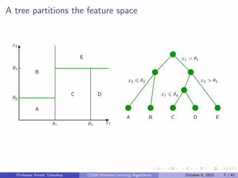
A tree partitions the feature space
A
B
C D
E
θ1 θ4
θ2
θ3
x1
x2
x1 > θ1
x2 > θ3
x1 6 θ4
x2 6 θ2
A B C D E
Professor Ameet Talwalkar CS260 Machine Learning Algorithms October 6, 2015 7 / 41
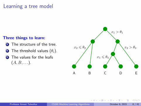
Learning a tree model
Three things to learn:
1 The structure of the tree.
2 The threshold values (θi).
3 The values for the leafs(A,B, . . .).
x1 > θ1
x2 > θ3
x1 6 θ4
x2 6 θ2
A B C D E
Professor Ameet Talwalkar CS260 Machine Learning Algorithms October 6, 2015 8 / 41
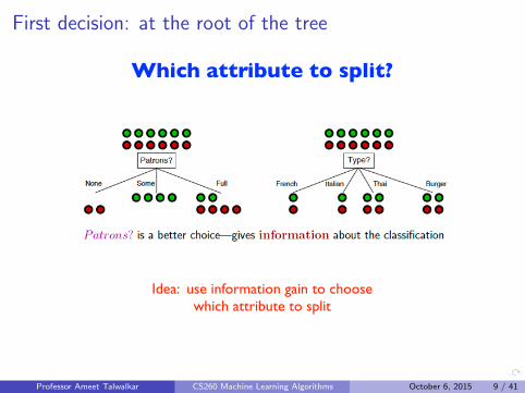
First decision: at the root of the tree
Which attribute to split?
Idea: use information gain to choose which attribute to split
Professor Ameet Talwalkar CS260 Machine Learning Algorithms October 6, 2015 9 / 41

How to measure information gain?
Idea:
Gaining information reduces uncertainty
!
Use to entropy to measure uncertainty
If a random variable X has K different values, a1, a2, ...aK, it is entropy is given by
!! H[X] = �
KX
k=1
P (X = ak) log P (X = ak)
the base can be 2 , though it is not essential (if the base is 2, the unit of the entropy is called
“bit”)
Professor Ameet Talwalkar CS260 Machine Learning Algorithms October 6, 2015 10 / 41

Examples of computing entropy
Entropy
0 1 2 3 4 50
0.2
0.4
0.6
0.8
1
Class
Probability
0 1 2 3 4 50
0.2
0.4
0.6
0.8
1
Class
Probability
0 1 2 3 4 50
0.2
0.4
0.6
0.8
1
Class
Probability
H(X) = 1.3863H(X) = 0.8360
H(X) = 0
Professor Ameet Talwalkar CS260 Machine Learning Algorithms October 6, 2015 11 / 41
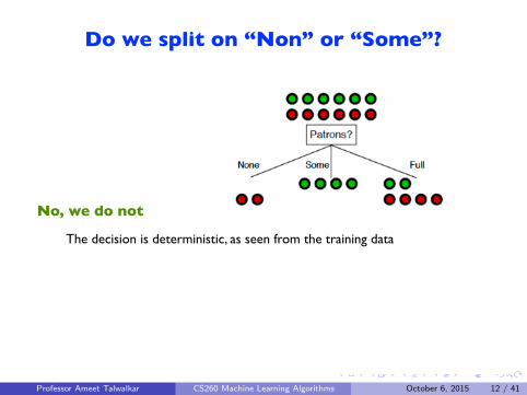
Do we split on “Non” or “Some”?
!
No, we do not
The decision is deterministic, as seen from the training data
Professor Ameet Talwalkar CS260 Machine Learning Algorithms October 6, 2015 12 / 41
What is the optimal Tree Depth?
We need to be careful to pick an appropriate tree depthI If the tree is too deep, we can overfitI If the tree is too shallow, we underfit
Max depth is a hyperparameter that should be tuned by the data
Alternative strategy is to create a very deep tree, and then to prune it(see Section 9.2.2 in ESL for details)
If leaves aren’t completely pure, we predict using majority vote
Professor Ameet Talwalkar CS260 Machine Learning Algorithms October 6, 2015 13 / 41

Example
Example
We stop after the root (first node)
!
!
!
!
!
!
!
Wait: yes Wait: noWait: no
Professor Ameet Talwalkar CS260 Machine Learning Algorithms October 6, 2015 14 / 41

Computational Considerations
Numerical Features
We could split on any feature, with any threshold
However, for a given feature, the only split points we need to considerare the the n values in the training data for this feature.
If we sort each feature by these n values, we can quickly compute ourimpurity metric of interest (cross entropy or others)
I This takes O(dn log n) time
Categorical Features
Assuming q distinct categories, there are 2q−1 − 1 possible partitionswe can consider.
However, things simplify in the case of binary classification (orregression), and we can find the optimial split (for cross entropy andGini) by only considering q − 1 possible splits (see Section 9.2.4 inESL for details).
Professor Ameet Talwalkar CS260 Machine Learning Algorithms October 6, 2015 15 / 41

Summary of learning trees
Advantages of using trees
Easily interpretable by human (as long as the tree is not too big)
Computationally efficient
Handles both numerical and categorical data
It is parametric thus compact: unlike NNC, we do not have to carryour training instances around
Building block for various ensemble methods (more on this later)
Disadvantages
Heuristic training techniquesI Finding partition of space that minimizes empirical error is NP-hardI We resort to greedy approaches with limited theoretical underpinnings
Professor Ameet Talwalkar CS260 Machine Learning Algorithms October 6, 2015 16 / 41

Outline
1 Administration
2 Review of last lecture
3 Naive BayesMotivating ExampleNaive Bayes ModelParameter Estimation
Professor Ameet Talwalkar CS260 Machine Learning Algorithms October 6, 2015 17 / 41

A daily battle
FROM THE DESK OF MR. AMINU SALEHDIRECTOR, FOREIGN OPERATIONS DEPARTMENTAFRI BANK PLCAfribank Plaza,14th Floormoney344.jpg51/55 Broad Street,P.M.B 12021 Lagos-Nigeria
Attention: Honorable Beneficiary,
IMMEDIATE PAYMENT NOTIFICATION VALUED AT US$10 MILLION
It is my modest obligation to write you this letter in regards to the authorization of your owed payment through our most respected financial institution (AFRI BANK PLC). I am Mr. Aminu Saleh, The Director, Foreign Operations Department, AFRI Bank Plc, NIGERIA. The British Government, in conjunction with the US GOVERNMENT, WORLD BANK, UNITED NATIONS ORGANIZATION on foreign payment matters, has empowered my bank after much consultation and consideration, to handle all foreign payments and release them to their appropriate beneficiaries with the help of a representative from Federal Reserve Bank.
To facilitate the process of this transaction, please kindly re-confirm the following information below:
1) Your full Name and Address:2) Phones, Fax and Mobile No. :3) Profession, Age and Marital Status:4) Copy of any valid form of your Identification:
I’m going to be rich!!
Professor Ameet Talwalkar CS260 Machine Learning Algorithms October 6, 2015 18 / 41

How to tell spam from ham?
FROM THE DESK OF MR. AMINU SALEHDIRECTOR, FOREIGN OPERATIONS DEPARTMENTAFRI BANK PLCAfribank Plaza,14th Floormoney344.jpg51/55 Broad Street,P.M.B 12021 Lagos-Nigeria
Attention: Honorable Beneficiary,
IMMEDIATE PAYMENT NOTIFICATION VALUED AT US$10 MILLION
Dear Ameet,
Do you have 10 minutes to get on a videocall before 2pm?
Thanks,
Stefano

How might we create features?
Professor Ameet Talwalkar CS260 Machine Learning Algorithms October 6, 2015 19 / 41

Intuition
Spam emails
we expect to see words like “money”, “free”, “bank account”, “viagra”
Ham emails
word usage is more spread out with few ‘spammy’ words
Q: How might a human solve this problem?
A: Simple strategy would be to look for keywords that we often associate with spam

Simple strategy: count the words
�⇧⇧⇧⇧⇧⇧⇤
free 100money 2
......
account 2...
...
⇥⌃⌃⌃⌃⌃⌃⌅
�⇧⇧⇧⇧⇧⇧⇤
free 1money 1
......
account 2...
...
⇥⌃⌃⌃⌃⌃⌃⌅
Bag-of-word representationof documents (and textual data)
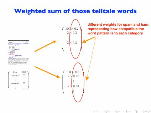
Weighted sum of those telltale words
�⇧⇧⇧⇧⇧⇧⇤
free 100money 2
......
account 2...
...
⇥⌃⌃⌃⌃⌃⌃⌅
�⇧⇧⇧⇧⇧⇧⇤
100 � 0.22 � 0.3
...2 � 0.3
...
⇥⌃⌃⌃⌃⌃⌃⌅
�⇧⇧⇧⇧⇧⇧⇤
100 � 0.012 � 0.02
...2 � 0.01
...
⇥⌃⌃⌃⌃⌃⌃⌅
different weights for spam and ham:representing how compatible the word pattern is to each category

Weighted sum of those telltale words
�⇧⇧⇧⇧⇧⇧⇤
free 100money 2
......
account 2...
...
⇥⌃⌃⌃⌃⌃⌃⌅
�⇧⇧⇧⇧⇧⇧⇤
100 � 0.22 � 0.3
...2 � 0.3
...
⇥⌃⌃⌃⌃⌃⌃⌅
�⇧⇧⇧⇧⇧⇧⇤
100 � 0.012 � 0.02
...2 � 0.01
...
⇥⌃⌃⌃⌃⌃⌃⌅
= 3.2
= 1.03
different weights for spam and ham:representing how compatible the word pattern is to each category

Our intuitive model of classification
Assign weight to each word
Compute compatibility score to “spam”
# of “free” x afree + # of “account” x aaccount + # of “money” x amoney
Compute compatibility score to “ham”:
# of “free” x bfree + # of “account” x baccount + # of “money” x bmoney
Make a decision:
if spam score > ham score then spam
else ham

How do we get the weights?
Professor Ameet Talwalkar CS260 Machine Learning Algorithms October 6, 2015 20 / 41

How do we get the weights?
Learn from experience
get a lot of spams
get a lot of hams
But what to optimize?

A probabilistic modeling perspective
Naive Bayes model for identifying spam
Class label: binary
y = {spam, ham}
Features: word counts in the document (Bag-of-word)
Ex: x = {(‘free’, 100), (‘lottery’, 10), (‘money’, 10), , (‘identification’, 1)...}
Each pair is in the format of(wi, #wi), namely, a unique word in the dictionary, and the number of times it shows up
Professor Ameet Talwalkar CS260 Machine Learning Algorithms October 6, 2015 21 / 41

Naive Bayes Model (Intuitively)
Features: word counts in the document
Ex: x = {(‘free’, 100), (‘identification’, 2), (‘lottery’, 10), (‘money’, 10), ...}
Model: Naive Bayes (NB)
p(x|spam) = p(’free’|spam)100p(’identification’|spam)2
p(’lottery’|spam)10p(’money’|spam)10 · · ·6= p(x|ham)

Naive Bayes Model (Intuitively)
Features: word counts in the document
Ex: x = {(‘free’, 100), (‘identification’, 2), (‘lottery’, 10), (‘money’, 10), ...}
Model: Naive Bayes (NB)
Parameters to be estimated are conditional probabilities: p(‘free’|spam), p(‘free’|ham),etc
p(x|spam) = p(’free’|spam)100p(’identification’|spam)2
p(’lottery’|spam)10p(’money’|spam)10 · · ·6= p(x|ham)
Naive Bayes Model
Intuitively this makes some sense (even if it seems simple)
We’ll now discuss the following:I Formal modeling assumptions for NB, and why it’s ‘naive’I NB classification rule converges to Bayes Optimal under these
assumptionsI How to estimate model parameters
Professor Ameet Talwalkar CS260 Machine Learning Algorithms October 6, 2015 22 / 41

Naive Bayes Model
These conditional probabilities are model parameters
Recall that each data point is a tuple (wi, #wi), namely, a unique dictionary word and the # of times it shows up
p(x|y) = p(w1|y)#w1p(w2|y)#w2 · · · p(wm|y)#wm
=�
i
p(wi|y)#wi

What is naive about this?
Professor Ameet Talwalkar CS260 Machine Learning Algorithms October 6, 2015 23 / 41

Strong assumption of conditional independence:
Previous example:
This assumption makes estimation much easier (as we’ll see)
p(wi, wj |y) = p(wi|y)p(wj |y)
Why is this ‘Naive’
p(x|spam) = p(’free’|spam)100p(’identification’|spam)2
p(’lottery’|spam)10p(’money’|spam)10 · · ·6= p(x|ham)

Naive Bayes classification rule
For any document x, we want to compare
p(spam|x) and p(ham|x)
Recall that Bayes Optimal classifier uses the posterior probability
f∗(x) ={
1 if p(y = 1|x) ≥ p(y = 0|x)0 if p(y = 1|x) < p(y = 0|x)
NB classification rule looks like the Bayes Optimal classifier under theassumption of conditional independence we just described
Professor Ameet Talwalkar CS260 Machine Learning Algorithms October 6, 2015 24 / 41

Naive Bayes classification rule
For any document x, we want to compare
p(spam|x) and p(ham|x)
Using Bayes rule, this gives rise to
p(spam|x) = p(x|spam)p(spam)
p(x), p(ham|x) = p(x|ham)p(ham)
p(x)
It is convenient to compute the logarithms, so we need only to compare
log[p(x|spam)p(spam)] versus log[p(x|ham)p(ham)]
as the denominators are the same
Professor Ameet Talwalkar CS260 Machine Learning Algorithms October 6, 2015 25 / 41
Classifier in the linear form
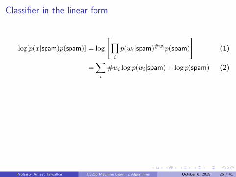
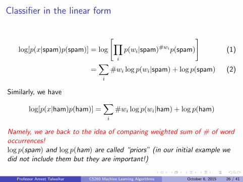
log[p(x|spam)p(spam)] = log
[∏
i
p(wi|spam)#wip(spam)
](1)
=∑
i
#wi log p(wi|spam) + log p(spam) (2)
Similarly, we have
log[p(x|ham)p(ham)] =∑
i
#wi log p(wi|ham) + log p(ham)
Namely, we are back to the idea of comparing weighted sum of # of wordoccurrences!log p(spam) and log p(ham) are called “priors” (in our initial example wedid not include them but they are important!)
Professor Ameet Talwalkar CS260 Machine Learning Algorithms October 6, 2015 26 / 41
Classifier in the linear form
log[p(x|spam)p(spam)] = log
[∏
i
p(wi|spam)#wip(spam)
](1)
=∑
i
#wi log p(wi|spam) + log p(spam) (2)
Similarly, we have
log[p(x|ham)p(ham)] =∑
i
#wi log p(wi|ham) + log p(ham)
Namely, we are back to the idea of comparing weighted sum of # of wordoccurrences!log p(spam) and log p(ham) are called “priors” (in our initial example wedid not include them but they are important!)
Professor Ameet Talwalkar CS260 Machine Learning Algorithms October 6, 2015 26 / 41

Mini-summary
What we have shownBy assuming a probabilistic model (i.e., Naive Bayes), we are able toderive a decision rule that is consistent with our intuition
Our next step is learn the parameters from dataWhat are the parameters to learn?
Professor Ameet Talwalkar CS260 Machine Learning Algorithms October 6, 2015 27 / 41
Formal definition of Naive Bayes
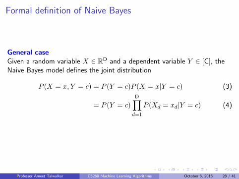
General caseGiven a random variable X ∈ RD and a dependent variable Y ∈ [C], theNaive Bayes model defines the joint distribution
P (X = x, Y = c) = P (Y = c)P (X = x|Y = c) (3)
= P (Y = c)
D∏
d=1
P (Xd = xd|Y = c) (4)
Professor Ameet Talwalkar CS260 Machine Learning Algorithms October 6, 2015 28 / 41
Special case (i.e., our model of spam emails)
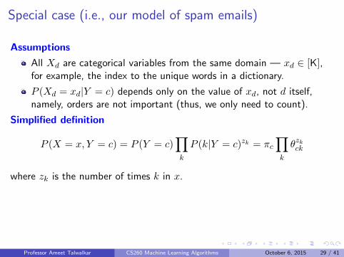
Assumptions
All Xd are categorical variables from the same domain — xd ∈ [K],for example, the index to the unique words in a dictionary.
P (Xd = xd|Y = c) depends only on the value of xd, not d itself,namely, orders are not important (thus, we only need to count).
Simplified definition
P (X = x, Y = c) = P (Y = c)∏
k
P (k|Y = c)zk = πc∏
k
θzkck
where zk is the number of times k in x.
Note that we only need to enumerate in the product, the index to the xd’spossible values. On the previous slide, however, we enumerate over d aswe do not have the assumption there that order is not important.
Professor Ameet Talwalkar CS260 Machine Learning Algorithms October 6, 2015 29 / 41

Special case (i.e., our model of spam emails)
Assumptions
All Xd are categorical variables from the same domain — xd ∈ [K],for example, the index to the unique words in a dictionary.
P (Xd = xd|Y = c) depends only on the value of xd, not d itself,namely, orders are not important (thus, we only need to count).
Simplified definition
P (X = x, Y = c) = P (Y = c)∏
k
P (k|Y = c)zk = πc∏
k
θzkck
where zk is the number of times k in x.Note that we only need to enumerate in the product, the index to the xd’spossible values. On the previous slide, however, we enumerate over d aswe do not have the assumption there that order is not important.
Professor Ameet Talwalkar CS260 Machine Learning Algorithms October 6, 2015 29 / 41
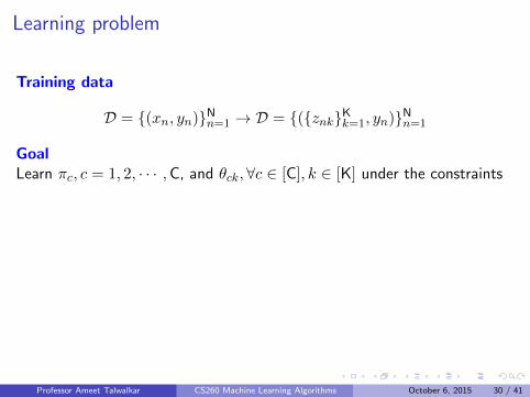
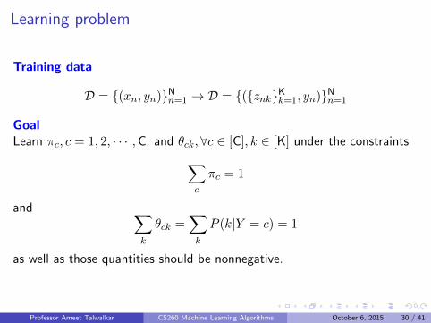
Learning problem
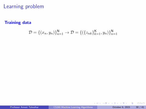
Training data
D = {(xn, yn)}Nn=1 → D = {({znk}Kk=1, yn)}Nn=1
GoalLearn πc, c = 1, 2, · · · ,C, and θck,∀c ∈ [C], k ∈ [K] under the constraints
∑
c
πc = 1
and ∑
k
θck =∑
k
P (k|Y = c) = 1
as well as those quantities should be nonnegative.
Professor Ameet Talwalkar CS260 Machine Learning Algorithms October 6, 2015 30 / 41
Learning problem
Training data
D = {(xn, yn)}Nn=1 → D = {({znk}Kk=1, yn)}Nn=1
GoalLearn πc, c = 1, 2, · · · ,C, and θck,∀c ∈ [C], k ∈ [K] under the constraints
∑
c
πc = 1
and ∑
k
θck =∑
k
P (k|Y = c) = 1
as well as those quantities should be nonnegative.
Professor Ameet Talwalkar CS260 Machine Learning Algorithms October 6, 2015 30 / 41

Our hammer: maximum likelihood estimation
Recall our joint probability
P (X = x, Y = c) = πc∏
k
θzkck
where zk is the number of times k in x.
Likelihood of the training data
D = {(xn, yn)}Nn=1 → D = {({znk}Kk=1, yn)}Nn=1
L = P (D) =N∏
n=1
πynP (xn|yn)
Professor Ameet Talwalkar CS260 Machine Learning Algorithms October 6, 2015 31 / 41

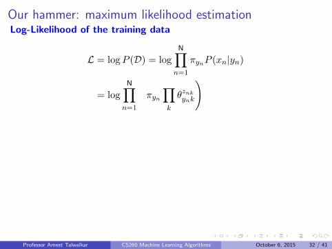
Our hammer: maximum likelihood estimationLog-Likelihood of the training data
L = logP (D) = log
N∏
n=1
πynP (xn|yn)
= log
N∏
n=1
(πyn
∏
k
θznkynk
)
=∑
n
(log πyn +
∑
k
znk log θynk
)
=∑
n
log πyn +∑
n,k
znk log θynk
Optimize it!
(π∗c , θ∗ck) = argmax
∑
n
log πyn +∑
n,k
znk log θynk
Professor Ameet Talwalkar CS260 Machine Learning Algorithms October 6, 2015 32 / 41

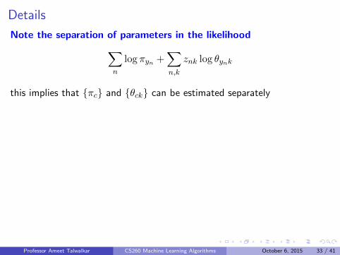
Details
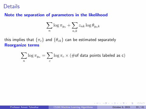
Note the separation of parameters in the likelihood
∑
n
log πyn +∑
n,k
znk log θynk
this implies that {πc} and {θck} can be estimated separatelyReorganize terms
∑
n
log πyn =∑
c
log πc × (#of data points labeled as c)
and
∑
n,k
znk log θynk =∑
c
∑
n:yn=c
∑
k
znk log θck =∑
c
∑
n:yn=c,k
znk log θck
The later implies {θck and {θc′k for c 6= c′ can be estimated independently(this is why our conditional independence assumption is so useful!).
Professor Ameet Talwalkar CS260 Machine Learning Algorithms October 6, 2015 33 / 41
Details
Note the separation of parameters in the likelihood
∑
n
log πyn +∑
n,k
znk log θynk
this implies that {πc} and {θck} can be estimated separately
Reorganize terms
∑
n
log πyn =∑
c
log πc × (#of data points labeled as c)
and
∑
n,k
znk log θynk =∑
c
∑
n:yn=c
∑
k
znk log θck =∑
c
∑
n:yn=c,k
znk log θck
The later implies {θck and {θc′k for c 6= c′ can be estimated independently(this is why our conditional independence assumption is so useful!).
Professor Ameet Talwalkar CS260 Machine Learning Algorithms October 6, 2015 33 / 41
Details
Note the separation of parameters in the likelihood
∑
n
log πyn +∑
n,k
znk log θynk
this implies that {πc} and {θck} can be estimated separatelyReorganize terms
∑
n
log πyn =∑
c
log πc × (#of data points labeled as c)
and
∑
n,k
znk log θynk =∑
c
∑
n:yn=c
∑
k
znk log θck =∑
c
∑
n:yn=c,k
znk log θck
The later implies {θck and {θc′k for c 6= c′ can be estimated independently(this is why our conditional independence assumption is so useful!).
Professor Ameet Talwalkar CS260 Machine Learning Algorithms October 6, 2015 33 / 41

Estimating {πc}
We want to maximize
∑
c
log πc × (#of data points labeled as c)
Intuition
Similar to roll a dice (or flip a coin): each side of the dice shows upwith a probability of πc (total C sides)
And we have total N trials of rolling this dice
Solution
π∗c =#of data points labeled as c
N
Professor Ameet Talwalkar CS260 Machine Learning Algorithms October 6, 2015 34 / 41
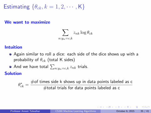
Estimating {θck, k = 1, 2, · · · ,K}
We want to maximize
∑
n:yn=c,k
znk log θck
Intuition
Again similar to roll a dice: each side of the dice shows up with aprobability of θck (total K sides)
And we have total∑
n:yn=c,k znk trials.
Solution
θ∗ck =#of times side k shows up in data points labeled as c
#total trials for data points labeled as c
Professor Ameet Talwalkar CS260 Machine Learning Algorithms October 6, 2015 35 / 41
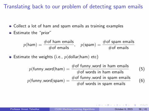
Translating back to our problem of detecting spam emails
Collect a lot of ham and spam emails as training examples
Estimate the “prior”
p(ham) =#of ham emails
#of emails, p(spam) =
#of spam emails
#of emails
Estimate the weights (i.e., p(dollar|ham) etc)
p(funny word|ham) =#of funny word in ham emails
#of words in ham emails(5)
p(funny word|spam) =#of funny word in spam emails
#of words in spam emails(6)
Professor Ameet Talwalkar CS260 Machine Learning Algorithms October 6, 2015 36 / 41

Classification rule
Given an unlabeled data point x = {zk, k = 1, 2, · · · ,K}, label it with
y∗ = argmaxc∈[C] P (y = c|x) (7)
= argmaxc∈[C] P (y = c)P (x|y = c) (8)
= argmaxc[log πc +∑
k
zk log θck] (9)
Professor Ameet Talwalkar CS260 Machine Learning Algorithms October 6, 2015 37 / 41

A short derivation of the maximum likelihood estimationTo maximize ∑
n:yn=c,k
znk log θck
We use the Lagrangian multiplier
∑
n:yn=c,k
znk log θck + λ
(∑
k
θck − 1
)
Taking derivatives with respect to θck and then find the stationary point( ∑
n:yn=c
znkθck
)+ λ = 0→ θck = − 1
λ
∑
n:yn=c
znk
Apply constraint∑
k θck = 1, plug in expression above for θck, solve for λ,and plug back into expression for θck:
θck =
∑n:yn=c znk∑
k
∑n:yn=c znk
Professor Ameet Talwalkar CS260 Machine Learning Algorithms October 6, 2015 38 / 41

Summary
You should know or be able to
What naive Bayes model isI write down the joint distributionI explain the conditional independence assumption implied by the modelI explain how this model can be used to classify spam vs ham emails
Be able to go through the short derivation for parameter estimationI The model illustrated here is called discrete/multinomial Naive BayesI HW2 asks you to apply the same principle to Gaussian naive BayesI The derivation is very similar – except there you need to estimate
Gaussian continuous random variables (instead of estimating discreterandom variables like rolling a dice)
Professor Ameet Talwalkar CS260 Machine Learning Algorithms October 6, 2015 39 / 41

Moving forward
Examine the classification rule for naive Bayes
y∗ = argmaxc log πc +∑
k
zk log θck
For binary classification, we thus determine the label based on the sign of
log π1 +∑
k
zk log θ1k −(log π2 +
∑
k
zk log θ2k
)
This is just a linear function of the features {zk}
w0 +∑
k
zkwk
where we “absorb” w0 = log π1 − log π2 and wk = log θ1k − log θ2k.
Professor Ameet Talwalkar CS260 Machine Learning Algorithms October 6, 2015 40 / 41

Naive Bayes is a linear classifier
Fundamentally, what really matters in deciding decision boundary is
w0 +∑
k
zkwk
This motivates many new methods. One of them is logistic regression, tobe discussed in next lecture.
Professor Ameet Talwalkar CS260 Machine Learning Algorithms October 6, 2015 41 / 41