image based diameter measurement and a …image based diameter measurement and ... 4.5 image...
TRANSCRIPT

IMAGE BASED DIAMETER MEASUREMENT AND
ANEURYSM DETECTION OF THE ASCENDING
AORTA
A THESIS SUBMITTED TO THE GRADUATE
SCHOOL OF APPLIED SCIENCES
OF
NEAR EAST UNIVERSITY
By
ŞERİFE KABA
In Partial Fulfillment of the Requirements for
the Degree of Master of Science
in
Biomedical Engineering
NICOSIA, 2017
IMA
GE
BA
SE
D D
IAM
ET
ER
ME
AS
UR
EM
EN
T A
ND
AN
EU
RY
SM
DE
TE
CT
ION
OF
TH
E A
SC
EN
DIN
G A
OR
TA
NE
U
2017
Ş
ER
İFE
KA
BA


IMAGE BASED DIAMETER MEASUREMENT AND
ANEURYSM DETECTION OF THE ASCENDING
AORTA
A THESIS SUBMITTED TO THE GRADUTE
SCHOOL OF APPLIED SCIENCES
OF
NEAR EAST UNIVERSITY
By
Şerife Kaba
In Partial Fulfillment of the Reguirements for the
Degree of Master of Science
in
Biomedical Engineering
NICOSIA, 2017
ŞERİFE KABA: IMAGE BASED DIAMETER MEASUREMENT AND
ANEURYSM DETECTION OF THE ASCENDING AORTA
Approval of Director of Graduate
School of Applied Sciences
Prof. Dr. Nadire ÇAVUŞ
We certify this thesis is satisfactory for the award of the degree of Masters of
Science in Biomedical Engineering
Examining Committee in Charge:
Prof. Dr. Hasan Demirel
Department of Electrical and Electronic
Engineering, EMU
Assist. Prof. Dr. Elbrus Imanov
Department of Computer Engineering,
NEU
Assist. Prof. Dr. Boran Şekeroğlu Department of Information Systems
Engineering, NEU

i
I hereby declare that all information in this document has been obtained and presented in
accordance with academic rules and ethical conduct. I also declare that, as required by these
rules and conduct, I have fully cited and referenced all material and results that are not
original to this work.
Name, Last name: Şerife Kaba
Signature:
Date:

ii
ACKNOWLEDGMENTS
Firstly, I would like to thank my supervisor Assist. Prof. Dr. Boran Şekeroğlu and co-
supervisor Assist. Prof. Dr. Hüseyin Hacı for their continuous support, help and knowledge.
Their patience, guidance and vast knowledge was extremely valuable to this work.
My deep gratitude goes to radiologist Dr. Enver Kneebone for giving me the idea for this
research topic and helping me in every possible way. This work would not have been
possible without him.
I want to acknowledge heart surgeon Assoc. Prof. Dr. Barçın Özcem and gynaecologist Dr.
Mustafa Sakallı for sharing their information.
I am grateful to “Letam Görüntüleme Merkezi’ (Medical Imaging Laboratory) and “Near
East University Hospital” for sharing the CT thorax (chest) scans from their database.
I especially thank Prof. Dr. Doğan İbrahim Akay and Dr. Umar Özgünalp for their support
and their good ideas. Also, I wish to thank all the engineering staff at Near East University.
Finally, I would like to thank my family and friends Sarah Ann Benstead, Deha Doğan,
Ahmet İlhan and Fatih Veysel Nurçin for their constant support during this work. I could not
have done this work without them.
iii
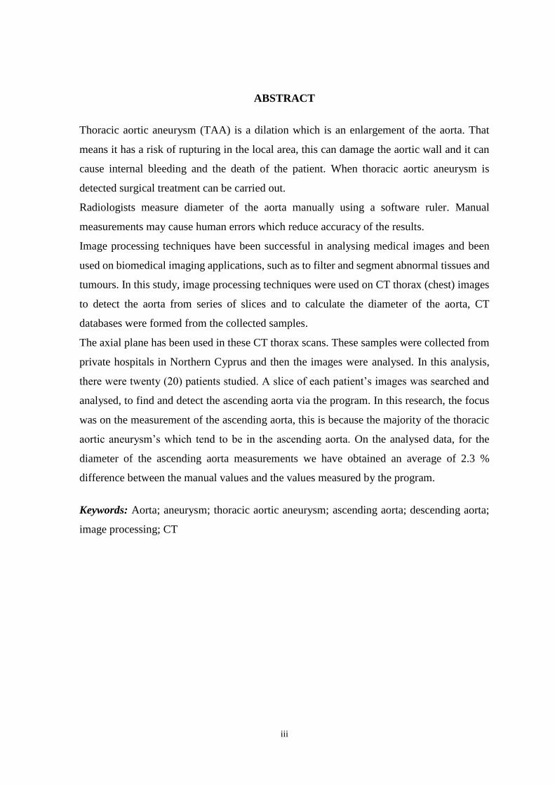
ABSTRACT
Thoracic aortic aneurysm (TAA) is a dilation which is an enlargement of the aorta. That
means it has a risk of rupturing in the local area, this can damage the aortic wall and it can
cause internal bleeding and the death of the patient. When thoracic aortic aneurysm is
detected surgical treatment can be carried out.
Radiologists measure diameter of the aorta manually using a software ruler. Manual
measurements may cause human errors which reduce accuracy of the results.
Image processing techniques have been successful in analysing medical images and been
used on biomedical imaging applications, such as to filter and segment abnormal tissues and
tumours. In this study, image processing techniques were used on CT thorax (chest) images
to detect the aorta from series of slices and to calculate the diameter of the aorta, CT
databases were formed from the collected samples.
The axial plane has been used in these CT thorax scans. These samples were collected from
private hospitals in Northern Cyprus and then the images were analysed. In this analysis,
there were twenty (20) patients studied. A slice of each patient’s images was searched and
analysed, to find and detect the ascending aorta via the program. In this research, the focus
was on the measurement of the ascending aorta, this is because the majority of the thoracic
aortic aneurysm’s which tend to be in the ascending aorta. On the analysed data, for the
diameter of the ascending aorta measurements we have obtained an average of 2.3 %
difference between the manual values and the values measured by the program.
Keywords: Aorta; aneurysm; thoracic aortic aneurysm; ascending aorta; descending aorta;
image processing; CT

iv
ÖZET
Torasik (Göğüs) ile ilgili aortik anevrizma aort damarının genişlemesinden dolayı oluşur.
Bu lokal alanda yırtılma riski olduğu anlamına gelmekle birlikte, aort duvarına zarar
verebilir ve iç kanamayla birlikte hastanın ölümüne sebep olabilir. Torasik ile ilgili aortik
anevrizmanın saptanmasında tıbbı müdahale gerçekleştirilmektedir.
Radyoloji uzmanları aort damarının çapını yazılım cetveli kullanarak el ile ölçerler. Elde
yapılan ölçümler, insan hatalarının ortaya çıkmasına neden olabilir ve bu da elde edilen
sonuçların hassasiyetini düşürür.
Medikal görüntü analizinde görüntü işleme teknikleri oldukça etkin yöntemler haline
gelmiştir. Bu teknikler biyomedikal görüntü uygulama-larında anormal dokuya sahip tümör
ve buna benzer diğer hastalıkları filtreleme ve ayırmak için kullanılmaktadır. Bu çalışmada,
görüntü işleme teknikleri CT toraks görüntüleri üzerinde aort damarını belirlemek ve çapını
hesaplamak için kullanılmış ve CT veri tabanı elde edilen örneklerle tablolandırılmıştır.
CT thorax taramalarında aksiyel kesit düzlemi kullanılmıştır. Bu örnekler Kuzey Kıbrıs`taki
özel hastanelerden toplanarak analiz edilmiştir. Bu analizlerde yirmi (20) hasta incelen-
miştir. Her hastanın görüntü kesitleri program aracılığı ile asendan (çıkan) ve desendan
(inen) aortayı belirlemek için araştırılmış ve analiz edilmiştir. Bir çok torasik ile ilgili aortik
anevrizma bu noktada oluşma eğiliminde olduğundan araştırmada odak nokta olarak
asendan aortanın ölçülmesi hedeflenmiştir. Analiz edilen veriler doğrultusunda asendan aort
çap ölçümleri için program ve manuel veriler arasında %2.3 fark belirlenmiştir.
Anahtar Kelimeler: Aorta; torasik aort; anevrizma; torasik aort anevrizma; asendan aort;
desendan aort; görüntü işleme; CT

v
TABLE OF CONTENTS
ACKNOWLEDGMENTS ……………...………………….…………………….……… ii
ABSTRACT…....……………………………………………………………………….... iii
ÖZET……………………………………………………………………………………... iv
TABLE OF CONTENTS………………………………………………………………... v
LIST OF TABLES……………………………………………………………….……. vii
LIST OF FIGURES……………………………….……………………………….…… viii
LIST OF ABBREVIATIONS…………………………………………………….……. ix
CHAPTER 1: INTRODUCTION
1.1 Aorta…….………………………….…...….………………………………………… 1
1.2 Aorta Related Diseases….……………………………………………………………. 3
1.3 Types of Aneurysm…………………………………………………………………….
1.4 Measuring the Size of Aorta.………………………………………………………….
1.5 The Aim of the Thesis………………………………………………………………….
1.6 Thesis Structure….…………………………………………………………………….
CHAPTER 2: BACKGROUND STUDY
2.1 Literature Review.………………………………………………………………….
CHAPTER 3: AORTA AND ITS BRANCHES
3.1 Anatomy of Aorta ….………………………………………………………………….
3.2 Histology of Aorta …………………………………………………………………….
3.2.1 The intima …………………………………………………………………………
3.2.2 The media …………………………………………………………………………
3.3.3 The adventitia.……………………………………………………………………
3.3 Imaging Modalities of Aorta ………………………………………………………….
CHAPTER 4: COMPUTER IMAGING AND DIGITAL IMAGE PROCESSING
4.1 Computer Imaging ...………………………………………………………………….
4.2 Image Analysis and Computer Vision ……………………………………………….
4.3 Image Processing ……………………………………………………………………...
4
6
7
7
9
15
17
18
18
19
19
22
23
23
vi
4.4 Computer Imaging Systems ………………………………………………………….
4.5 Image Formatting and Sensing ……………………………………………………….
4.6 Imaging Outside the Visible Range of the EM Spectrum …………………………...
4.7 Imaging Representation ………………………………………………………………
4.7.1 Binary images….…………………………………………………………………
4.7.2 Gray-scale images ……………………………………………………………….
4.7.3 Colour images ……………………………………………………………………
4.7.4 Multispectral images …………………………………………………………….
4.8 Digital images file formats …………………………………………………………...
CHAPTER 5: PROPOSED SYSTEM
5.1 Database…………...………………………………………………………………….
5.2 System ……………………………….………………………………………………...
5.2.1 Image binarization.………………………………………………………………...
5.2.2 Circular Hough transform ………………………………………………………....
5.2.3 Pixel to mm conversion ……………………………………………………………
CHAPTER 6: RESULTS AND DISCUSSION
6.1 Results …………………………………………………………………………………
6.2 Discussion …………………………………………………………………………….
CHAPTER 7: CONCLUSION AND SUGGESTIONS
7.1 Conclusion.……………………………………………………………………………
7.2 Suggestions…….………………………………………………………………………
REFERENCES ………………………………………………………………………….
25
26
27
29
30
30
30
31
31
33
34
35
37
40
47
58
60
61
62

vii
LIST OF TABLES
Table 1.1: Size of the Normal Adult Thoracic Aorta ……………………………………...
Table 5.1 Edge detectors available in function Edge ……………………………………
Table 6.1: Comparison of manually and automatically measured ascending aorta diameter
values and their difference ……………………………………………...........
6
42
47
viii
LIST OF FIGURES
Figure 3.1: Dorsal (back) view of the heart and its great vessels…...……………………
Figure 3.2: Segments of the aorta………………………………………………………….
Figure 3.3: Main components of the aorta…………………………………………………
Figure 3.4: Appearance of elastin sheets ………….……………………………………...
Figure 3.5: CTA images for aortic aneurysm……….…………………………………….
Figure 3.6: Axial - coronal two-dimensional images of CTA …....………………………
Figure 4.1: The hierarchical image pyramid………………………………………………
Figure 4.2a: X-ray chest image…………………………………………………………....
Figure 4.2b: Dental x-ray image………………………………………………………......
Figure 4.2c: Cell images ………………………………………………………………….
Figure 4.2d: Cell images………………………………………………………………….
Figure 4.2e: CT abdomen image ………………………………………………………….
Figure 4.3a: GOES image of North America……………………………………………...
Figure 4.3b: MRI shoulder image…………………………………………………………
Figure 5.1: Images of the database, CT Thorax (chest) patient samples ………………….
Figure 5.2: Block Diagram of the Proposed System ………………………………………
Figure 5.3: Examples of the CT thorax images for the first test patient……………………
Figure 5.4: Classical CHT voting pattern………………………………………………….
Figure 5.5: Circle detection of ascending aorta …………………………………………
Figure 5.6: Ruler and Pixel Information in CT Scans …………………………………….
Figure 5.7: Cropping of Region of Interest ………….…………………………………….
Figure 5.8: Binarization (4 cm scale) …………………………………………..................
Figure 5.9: Sobel Masks.………………………………………………………………...
Figure 5.10: Prewitt Masks……………………………………………………………….
Figure 5.11: Laplacian Masks…………………………………………………………….
Figure 5.12: Prewitt Operator Method…………………………………………………….
Figure 6.1: CT Thorax images of patient 1…………………….………………………….
Figure 6.2: Ascending Aorta Diameter Measurement for Patient 1 ………………………
Figure 6.3: CT Thorax images of patient 2……………………………………………….
Figure 6.4: CT Thorax images of patient 3……………………………………………….
16
17
18
18
20
21
26
28
28
28
28
28
29
29
33
34
36
37
39
40
41
41
42
43
43
44
50
51
55
58
ix
LIST OF ABBREVIATIONS
2D:
3D:
AAA:
AAOD:
AI:
BMP:
BSA:
CAC:
CAD:
CDC:
cm:
CT:
CTA:
EBT:
EM:
GOES:
GUI:
HT:
JPEG:
MATLAB:
mm:
MRF:
MRI:
NOAA:
PET:
RGB:
SIUE:
TAA:
TH:
UV:
Two-Dimensional
Three-Dimensional
Abdominal Aortic Aneurysm
Ascending Aortic Diameter
Artificial Intelligence
Bitmap
Body Surface Area
Coronary Artery Calcium
Coronary Artery Disease
Centres for Disease Control and Prevention
Centimetres
Computed Tomography
Coronary CT Angiography
Electron Beam Computed Tomography
Electromagnetic Spectrum
Geostationary Environment Satellite
Graphical User Interface
Hough Transform
Joint Photographic Experts Group
Matrix Laboratory
Millimetres
Markov Random Field
Magnetic Resonance Imaging
National Oceanic and Atmospheric Administration
Positron Emission Tomography
Red Green Blue
Southern Illinois University Edwardsville
Thoracic Aortic Aneurysm
Threshold
Ultraviolet

1
CHAPTER 1
INTRODUCTION
1.1 Aorta
The aorta is the widest and strongest artery in human body. It is a blood vessel which is
pumped by the heart through the lungs by oxygenated blood. The blood is delivered by
tributaries of the aorta to the whole body. It starts from to bottom part of the heart which
extends along upper part to the right up to the head, then continues down to the left lying
through the spine in the chest and upper abdomen before it is segmented into two parts for
each leg (O’Gara, 2003).
It has a three-layer wall. The wall is composed of thin inner layer or intima, the middle layer
or media which is thicker and the outer thinner layer or adventitia. The aortic intima is found
to be a very thin layer of tissue which is very fragile which means that it can be easily
damaged. The aortic intima’s structure has an endothelium-lining which is very sensitive.
The middle layer of the aorta is called the media, this media muscle is developed by the
fluent muscle action of the cells and its various layers of elastic laminae which gives it, it’s
great strength, versatility and stretching capacity, that creates its strength for the aorta to
process. The adventitia has different structures, these include collagen and vasa vasorum.
These structures aid in maintaining of the outer half of the aortic wall as well as the first
section of the media. The flexible and stretching structure of the aorta is significant for its
standard processing. The flexibility of the aorta is its valuable quality in being able to remove
any pulsing interference from the left ventricle as a systolic pulse and to control its strong
forward modulation during the diastolic pulse. Medical elastic fibres could get thinner and
break up due to aging. The lamine has a concentric structure and could be damaged because
of fragmentation of the elastic fibres. These undergoing circumstances are take place by the
increase of collagen and ground substance. The weakness of the elasticity in aorta’s wall
creates augmentation of pulse pressure mostly occurs in older people and could arise by
onward dilatation of the aorta (Goldstein et al., 2015).
The aorta should have a resisting structure for the pressure created by each heartbeat as well
as elasticity for delivering the blood to the other parts of the body. There are several

2
circumstances such as normal aging and hypertension that could damage or weakened the
wall of the aorta.
Moreover, if the gene which creates the elastic tissues is insufficient the structure of the wall
will be weak and thinner than the normal. The less common circumstances damaging the
wall could be stated as inflammation caused by certain white blood cells, infection, and
trauma. Atherosclerosis, high cholesterol that causes coronary artery disease damages the
inner part (endothelium) of the aorta and could weaken the wall. Atherosclerotic deposits
generally formed in the abdominal part just below the level of the segments lying to the
kidneys (O’Gara, 2003).
It’s important to remember that the aorta is the main artery in the human body, and so it’s
functioning ability is both as a channel for the passage of fluids as well as a storage vessel.
Its elastic properties allow it to enlarge during the systolic action of the heart and in the
recoiling of the diastolic action. It can be seen, that the left ventricular stroke volume is
stored in the ascending aorta, this can be up to fifty percent, (50 %), this action occurs at the
end of the systolic action of the aorta and the stored blood is then pushed surging forward
during the diastolic action of the aorta, into the peripheral circulation of the blood system.
This process is significant for blood flow and arterial pressure of the cardiac cycle. The
function of the reservoir is for the arterial pressure to keep a constant blood flow all the way
through the cardiac cycle, because the thoracic section of the aorta has more elastin, so it is
more able to elastically expand and carry out its many complex tasks then the abdominal
aorta. This elastic and flexible structure could diminish because of age and a disruption in
elastin and collagen depending upon several diseases. This decline of the elastic structure of
the wall could cause a rise of systolic pressure during left ventricular systole as well as an
enlargement and lengthening. The changes and disruption of the aortic wall, could be
identified by examining the volume of the aortic wall which is affected by the constant
current variations of the aortic pressure so it can be identified by its diameter or by the area
change in the cardiac cycle regarding to changes in pressure or by assessing the velocity of
the pulse wave in that specific area (Goldstein et al., 2015).
There are two main segments of the aorta which are abdominal and thoracic. The thoracic
aorta has three parts; descending, ascending and arch. The ascending aorta is between aortic
valve and innominate artery (branchiocephalictrunc). It is roughly 5 cm long and has two
specific segments. The lower segment is called aortic root which covers the sinuses of

3
Valsalva and sinotubular junction (STJ). Tubular ascending aorta is the upper segment which
starts at the STJ and reach out to the aortic arch (innominate artery).
Majority of the TAA are found at the ascending aorta which could influence both the aortic
root and tubular aortic segment (Saliba et al., 2015).
1.2 Aorta Related Diseases
There are several diseases which are directly related with aorta. One of these diseases is
aneurysm. An aneurysm is a kind of swelling in an artery. Arteries are bloods vessels that
transfer oxygen rich blood to the whole body.
Arteries have thick walls to resist normal blood pressure. These walls can be injured or
damaged by several medical problems, trauma and genetic condition. Damaged or injured
walls pressured by blood can any aneurysm. It can grow more, explode and shatter.
Serious bleeding can be cause inside the body explosion. When the layers of the artery wall
are separated into one or more layers it is called dissection. This creates a bleeding within
and along the wall layers of the artery. Explosion and dissection are often causes death
(National Heart, Lung, and Blood Institute).
Aneurysm is a serious disease which impairs the wall of the aorta. It is likely to cause, the
following disorders, smoking illnesses, gender genetic issues, age related illnesses, possibly
high blood pressure problems, disorders of the connective tissues, and the possibly family
history traits are the risk factors of having aortic aneurysm. Patients having aortic aneurysms
are generally at higher risk of aortic dissection regarding to their size, current medical
situation and genetics. An aortic dissection takes place due to layers of aorta splitting up
which leads to blood flowing into the layers. This damages aorta and may cause rupture
(Frankel Cardiovascular Center University of Michigan Health System).
Due to an occurrence of an abnormal canal within the aortic wall regarding to a deformation
of the intimal lining, aortic dissection happens. This may cause the following abnormalities:
Hypertension, cystic medial necrosis, connective tissue disorders such as Marfan syndrome,
metabolic disorders, crack cocaine use and iatrogenic are the main causes of the dissection,
atherosclerosis which is congestion of the vasa vasorum, Ehlers-Danlos syndrome and
finally pregnancy (Farelli and Dake, 2009).
When a sudden pain is felt at the midsternum, it often becomes very severe quite quickly,
this is usually due to the initial tear or even possibly due to dissection occurring at the

4
ascending aorta and usually in between the scapular area for the descending thoracic aortic
dissection. This type of pain is usually non-localised, when this occurs these symptoms
should be observed carefully because, this could be a sign of dissection extension, either as
a normal flow or a reverse flow of the aortic circulation. If the patient has an existing
aneurysm a painless dissection could occur and in the presence of a chronic aneurysm pain,
a new dissection pain could not be identified (Farelli and Dake, 2009). According to Farelli
and Dake (2009), hypotension, abdominal pain, intestinal or inferior limb ischemia and
bradycardia may have similar symptoms to dissection process.
It has been the scope of this thesis to specifically examine, research and study the ‘Ascending
type of aneurysm’.
1.3 Types of Aneurysm
There are two types of aortic aneurysm; thoracic aortic aneurysm and abdominal aortic
aneurysm (National Heart, Lung, and Blood Institute).
Abdominal aortic aneurysm is a kind of aneurysm formed in the abdominal part of the aorta.
Most aortic aneurysm is AAAs. Comparing the past these kinds of aneurysm are diagnosed
more often because of the use of computed tomography scans or CT scans. Small AAAs
does not fracture easily. But they can expand more without showing symptoms. This could
be avoided by frequent check-ups and treatments (National Heart, Lung, and Blood
Institute).
The second type of aneurysm is thoracic aortic aneurysm. This kind of aneurysm is formed
in chest area of the aorta which is on top of the diaphragm is called thoracic aneurysm (TAA).
Generally, it does not create any symptoms even when it is large. It is easily diagnosed
nowadays because of the use of chest CT scans. TAA is formed by a weakness on the wall
of aorta and an expansion of the part of aorta close to the heart. Therefore, this prevents the
valve between the heart and the aorta to close completely. So, the blood flows back into the
heart (National Heart, Lung, and Blood Institute).
An aneurysm occurs in the upper back away from the heart is a rarely seen type of TAA.
This could be generally formed from an injury of the chest such as car accident (National
Heart, Lung, and Blood Institute).
The most common aortic pathologies in relation to the thoracic aneurysm are disorders of
the connective tissues, these include Ehlers Danlors, Marfan syndrome, infection of the

5
aortic wall, also trauma, Takayasu’s arteritis, atherosclerosis, and idiopathic cystic medial
degeneration (Farelli and Dake, 2009).
In United States, TAA has ranked in the top 20 leading causes of death by its relevant
symptoms which is life threatening. (15th leading causes of death in people over 65 years
old). However, the death rate of patients carrying the symptoms of TAA has remained stable
in the last two decades compared to the patients having CAD (Saliba et al., 2015).
It is reported that possibility of having TAA is 5.9 cases in 100,000 people- years in the early
1980s however current technological equipment’s in imaging procedure, has proven that
because of aging of the population, increased use of transthoracic echocardiography and
routine screening, this ratio has been doubled. Regarding to the CDC, the ratio of patients
having ascending TAA is approximately 10 per 100,000 person-years. Gender estimation of
thoracic aortic aneurysm is equal where the age estimation at diagnosis is a decade higher in
woman (70s) than in men (60s) (Saliba et al., 2015).
Aneurysm can develop in certain parts of the thoracic aorta which includes the aortic curve
of the descending aorta in the lower section of the thoracic aorta, ascending aorta near the
heart (Mayo Clinic).
Ascending aortic aneurysms are usually leads to an aortic root dilation and infiltration of the
aortic valve in relation to insufficient oxygen where the heart could get weaker due to
insufficiency. Aortic arch aneurysms are more related to upper chest or interscapular back
pain. If it gets larger the esophagus and the airway could be compressed. The most common
signs are having difficulty in swallowing and / or hoarseness. Descending thoracic
aneurysms generally do not show any symptoms. They can cause a rare back pain (Farelli
and Dake, 2009).
Ascending aorta aneurysm is considered as a serious disease especially in overage people
since there is a high risk in medical intervention. It is a life-threatening disease which has to
be treated, and usually could not be diagnosed before dissection or rupture. Thus, early
diagnosis is always important. Most of the studies show that the risk of medical intervention
could be acceptable regarding to the possibility of death from chronic or asymptomatic
disease. The maximum diameter of an aneurysm is 6 cm and reports show that the percentage
of rupture, dissection or death from aneurysm is %14.1 (Lohse et al., 2009).

6
1.4 Measuring the Diameter of Aorta
The techniques and methods used for measuring the size of aorta as well as the size are
crucial issues for diagnosing relevant diseases. In reviewing aorta and aortic root, surgical
methods that not requires incision such as radiography, computed tomography (CT),
echocardiography and magnetic resonance imaging (MRI), are the primary diagnosing
methods before using catheter-based angiography which is a surgical operation (Boxt and
Abbara, 2015).
Diagnosing circumstances of thoracic aorta and the aortic root needs imaging in order to
measure the dimensions of the aortic annulus, assigning stenoses and the expansiveness of
the aorta, abnormal sores to the cardiac chambers or systemic vessels (Boxt and Abbara,
2015).
One of the most important issues of identifying aortic disease is the size of aorta. The
absolute distance between the left border of the trachea and the subsidiary border of the
aortic arch should not be more than 4 cm on the frontal chest radiography for adults. This
measure is generally less than 3 cm for people not older than 30 years’ age. The admissible
diameter of the ascending aorta should not be more than 4 cm on an aortogram or
tomography. An aneurysm could occur at the ascending thoracic aorta if the dimension is
more than 5 cm where an aneurysm at the descending aorta emerges if the dimension is
greater than 4 cm. Generally, the scale of the aorta of healthier people differs and increases
according to age (Boxt and Abbara, 2015).
Table 1.1: Diameter of the Normal Adult Thoracic Aorta (Boxt and Abbara, 2015)
Mean (cm) Upper Limit of Normal*(cm)
Aortic root 3.7 4.0
Ascending aorta 3.2 3.7
Descending aorta 2.5 2.8

7
1.5 The Aim of the Thesis
Aim of this thesis is to determine diameter of ascending aorta to identify aortic aneurysm.
Identification of aorta diameter is vital to treat patient according to the current situation of
the patient which includes types of treatment to be chosen or surgical intervention. The
system designed in this thesis has been created to automatically detect diameter of ascending
aorta. MATLAB environment has been used to create this system. Image processing
techniques have been carried out to perform following tasks. In first step image binarization
has been applied to convert RGB into binary image. Thus, it has been enabled for the aorta
in the image (ascending) to be seen more clearly. Then, circular Hough transform method
were used to detect and measure the diameter of the aorta. In next step, the lines on the image
that scale for 4 cm were detected by Hough transform. Then those areas cover 4 cm were
calculated in pixel values and then converted into millimetres. The aortas location was
determined by the value of the y coordinate situated in the centre point of the aorta. In the
CT thorax images, the top of the images shows the ascending aorta and the bottom shows
the descending aorta.
The main aim of this thesis is to provide a system that can obtain accurate and reliable results
while measuring the aorta automatically compared to the manual techniques which is used
by radiologists. This technique is more accurate, decreases human based errors, requires less
time, provides worldwide service through online systems especially in developing countries
and in the presence of specialist doctors creates an advantage to take necessary actions in
advance and on time.
1.6 Thesis Overview
Main parts of the thesis are as shown below:
• Chapter 1 presents the introduction to the thesis.
• Chapter 2 presents the literature review of this study.
• Chapter 3 explains anatomical information, related diseases, imaging modalities
and measurement techniques of the aorta.
• Chapter 4 gives general information related to the computer imaging and the
image processing techniques.
• Chapter 5 is the methods that were used in this thesis.

8
• Chapter 6 is the results and discussion.
• Chapter 7 is the conclusion and suggestions part of this thesis.

9
CHAPTER 2
BACKGROUND STUDY
2.1 Literature Review
In the research of Rueckert et al. (1997), deformable models have been used to observe the
cardiovascular activity of the aorta by using MR images. Through using the initial data
researches have applied multi-scale response function to measure the diameter and the
location of the aorta. An assessment has been made with the measurements obtained by the
developed method called Markov-random-field, MRF framework. As a result, the
framework has created an algorithm and accuracy as well as efficient results which
contributed clinical treatments.
A method was designed by Adame et al. (2006) for automatically detecting the vessel wall
contour and measuring the thickness of the wall of aorta through In-Vivo MR images. The
purpose of this method is to form an automatic application for observing the luman contour
and the outer surrounding of the aortic wall. The method contributes to quantification of the
thickness of the wall through axial MR images. The materials and methods include algorithm
which uses previous data of vessel wall morphology. In order to obtain an approximate
measure of the contours a geometrical method is translated and rotated. Through measuring
the gap between inner and outer contour of the wall, the thickness of the wall was calculated.
This algorithm is a strong technique for drawing the boundaries of the wall and measuring
the thickness automatically.
Kovaks et al. (2006) have created a method which automatically segments the vessel lumen
from 3D imaging of aortic dissection. According to Kovaks et al. (2006), a Computer Aided
Diagnosing system which can easily and instantly discovers different lumens is not created
yet. However, the method they have created is a first attempt for such a system which could
segment the whole aorta automatically. The method is resistive for lack of homogeneity
during distribution of contrast agent usually occurs in the dissection membrane sectioning
true and false lumen, dissected aorta, as well as high density artifacts. The method was
applied over HTs to find the exact spherical form of the aorta on the different sections which
are vertical to the vessel as well as 3D is used for adjusting the identified contour to the
aortic lumen.

10
The study by Wolak et al. (2008) emphasized the determination of normal limits for
ascending and descending thoracic aorta dimensions by aiming patients under low risk and
cases that has no significant symptoms. The diameter of the ascending and descending aorta
could be measured by gated noncontrast computed tomography scans applied for coronary
calcium assessments. The method was applied by measuring descending and ascending
thoracic aorta dimension at the level of pulmonary artery bifurcation with people having
coronary artery calcium scanning. In order to estimate the risk factors related individually
with ascending and descending thoracic aorta diameter, multiple linear regression analysis
is used. The outcome of linear regression is used to form a formula of BSA versus
nomograms of aortic diameter related to age groups where this calculates the size over age,
gender through the estimation of the aortic size. As a result, it was stated that age, BSA,
hypertension and gender were completely related with the dimensions of thoracic aorta.
Moreover, patients also having diabetics were related with ascending aorta diameter and
patients with smoking habits were associated with descending aorta diameter. This study
summarised that normal limits of descending and ascending aortic dimensions obtained by
Computed Tomography, have been examined by BSA, age, gender and regarding patients
under low risk of requiring CAC Scan.
According to Kurkure et al. (2008) the calcification of aorta is related to cardiovascular
disease. In order to measure and identify the amount of calcium in aorta a novel method has
been presented in the study for asserting and segmenting the thoracic aorta by using non-
contrast CT images. This process has been formulated as optimal path identifying problems
which are solved through the usage of dynamic programming. For segmentation and
localization of aorta, several methods have been used on Hough space. In order to evaluate
the process, comparisons have been made with manual detections over viewing volume
overlap, boundary disease and the location of the aorta. As a result of using dynamic
programming-based to localize and segment the aorta automatically, it is shown that the
process is more efficient compared to the popular method of selecting the point of global
maxima in the Hough space.
Mao et al. (2008) has introduced a study to assemble the standard metric of ascending aortic
diameter AAOD through measuring it with Electron Beam Computed Tomography (EBT)
and 64 Multi-Detector Computed Tomography (MDCT) reliant upon gender and age
differences. The results have presented an important linear relation with gender, age,

11
pulmonary artery diameter and descending aortic diameter. The diameter of ascending aorta
rises related to male gender and age. In order to separate the pathologic atherosclerotic
variations in the ascending aorta the measures of aortic diameters made though gender and
age specification are highly necessary.
Dehmeshki et al. (2009) has developed a Computer-aided detection system in order to get
more efficient results by performing automatic and accurate detections of abdominal aortic
aneurysm. Firstly, the system assigns and extracts the lumen in order to identify the location
of the abdominal aortic. The abdominal aortic lumen which has been extracted is then used
as an initial surface for segmentation of aorta to detect aneurysm. The structure of lumen
and aorta has been studied for detecting aneurysm regarding the normal expected variation
of the aorta. The results of the measurements done by the system presents, 98 % success on
detection depending on 60 CTA datasets and 95% success in segmentation.
In the study of Tokuyasu et al. (2009) an approach of detecting the region of artery with the
arterial tissues shown on tomographic images of patient has been introduced. The aim is to
provide diagnosis support system for thoracic arterial disease mostly for arch aorta aneurysm
where it is difficult to estimate the shape and the statement of aneurysm during operation for
surgeons using latest medical imaging methods.
The researchers have created an instructional report by investigating the changes in the size
of the ascending aorta by using electrocardiograph-gated multi-detector computerised
tomography which is supported by computer software. As a result, the use of CAD reduces
the variability of diameter measurements in the detection of the ascending aorta. The results
of the study show that the maximal variability gained by ECG-gated MDCT angiography
was 1.2m where this should be accounted in the measurement of thoracic aorta (Lu et al.,
2009).
The study of Al-Agamy et al. (2010) presents an algorithm to segment the ascending and
descending aorta from magnetic resonance flow images. The algorithm relies on the active
contour model including several corrections. Through this algorithm, faults in segmentation
resulted from severe image artifacts have been detected and corrected automatically. The
algorithm provides three significant advantages; it is operating fast, there is no need for
maximum user interaction and it is resistant to the changes in parameters.
Maria and Tiberiu (2013) have studied possible techniques and methods of medical imaging
to detect aortic aneurysm and dissection through image segmentation. The software called
12
MATLAB which contributes to design a new graphical user interface as well as practising
and analysing the method has been used for influential segmentation of images gained
through threshold method. This application also provides an integrated environment GUIDE
which is user friendly and the images collected through any of the recent imaging methods
could be segmented as mono or fuzzy modes while examining aortic aneurysm. This method
focuses on detecting aortic aneurysm and dissection by creating a new graphical user
interface GUI which uses the integrated development environment for graphical interfaces
GUIDE function of MATLAB software.
The study implemented by Lohou et al. (2013) has revealed a global image processing
framework for planning the treatment and providing support for ascending aorta dissections.
Computed Tomography Angiography technique was used to reveal the characteristics of the
aortic dissection. Firstly, the method has contributed the extraction of aortic dissection stages
which helped the planning of clinical treatments. Secondly, the method has provided related
visual images of the ascending aorta which can be used for assistance during clinical
surgeries.
Entezari et al. (2013) have investigated a method to examine the thoracic aorta using semi-
automated post processing tool. They have implemented a manual technique and semi-
automated software. They have also measured the time acquisition of the method developed.
The measurement results show that the vessel dimension of the thoracic aorta gained by
semi-automated method was feasible in comparison to commonly used manual technique.
The method applied was also created an advantage of reducing post-processing time.
Muraru et al. (2013) have used various imaging of two-dimensional echocardiography to
measure ascending aorta diameters on 2018 healthy people. They have found out that the
ascending aorta diameter is smaller in terms of inner edge convention. Also, the study has
proved that to estimate ascending aorta pathology values depending on gender for ascending
aorta diameter in index for body surface area should be used.
The objective of the study of Rudarakanchana et al. (2013) was to investigate and analyse
the variation in descending thoracic aortic aneurysm diameters measured on CT scans in
different area by different specialists and to find the effect on making treatment decisions.
The highest corrected measurements of diameter were smaller than axial measurements.
According to the study this could be measured by a continuous process with minimum inter-
observer variability.

13
Montes et al. (2013) have used a method in order to segmentation, extract the centreline and
localize the thoracic aorta by using cardiac computed tomography imaging technique to be
able to visualize calcification of the aorta. They have obtained efficient data by this method
on cardiac CT images which was promising.
Aorta dissection is a serious vascular disease which is formed by a tear of the tunica intima
of the vessel wall which is life threatening to the patient. One of the most common
diagnosing methods is multi-detector CT which is based on imaging of the aorta. The aim
of the study carried out by Krissian et al. (2013) was to develop semi-automatic detection
tool. They proposed two staged method. First method was semi-automatic extraction of the
aorta and its parts to segment the outer wall of the aorta by using geodesic-level set
framework. The second method was developed to detect the centre of the dissected wall
through original algorithm based on the zero crossing two vector areas. The model provides
specialist a new and interesting tool to create more attention on medical image processing.
The aim of the study established by Mera et al. (2014) was to classify thoracic aortic
aneurysm automatically using CT images. The researchers focused on the improvement of
an automatic technique to detect the calibre of the thoracic aorta. They have compared the
method with the gold standard commercial software. In terms of clinical cases a good
relationship was found between the method they use and the gold standard. And the ANOVA
(Analysis of variance) test results exhibited that there was no statistically difference where
f=1.88 and p=0.153.
Horikoshi et. al. (2014) have developed an automated recognition technique by using
thoracic Multi-Slice CT images to diagnose aorta aneurysm. This technique gives variety of
information such as the skeleton of thoracic aorta, the actual place of the aneurysm and the
diameter of each cross-section along the skeleton. The information help professionals to
design a stent and place it perfectly to the aorta aneurysm area where the original position
against the blood stream is kept by the stent. An algorithm of Successive Region Growing
has been applied to extract the 3D shape of the aorta.
Aortic size assessment and segmentation were studied by different approaches and different
techniques among researchers. Thoracic Aorta size can be measured manually by
semiautomatic diameters and double oblique short axis views from centreline investigation
in daily clinical practice. The method which is double oblique was achieved by radiologists
in advanced image processing workstations and semiautomatic diameter analysis is

14
performed in dedicated 3D imaging lab. The measurement purpose is to find largest diameter
in the thoracic aorta. All measurements are rounded to nearest mm (Quint et al., 2014).
Sobotnicka et al. (2016) have used split/merge method on computed tomography aorta
images. This method involved using image processing techniques. By using this automatic
method, it provided a way to split those elongated structures of the anatomy (in this case the
aorta) is split into smaller sections, which have regions that have pixels of the same
concentration level. The evaluated image was first processed than it was filtered. Initial
image processing is the first step of image analysis in this study. A median filter was applied
to filtrate the image. After the image filtration, binarization (thresholding) method was used.
Later the image was segmented by using split/merge method and then statistically analysed
and the image features were interpreted. Therefore, this study reflects the way an image
processing is determined, that is, first its numerically and then symbolically determined.
15
CHAPTER 3
AORTA AND ITS BRANCHES
3.1 Anatomy of Aorta
In the body, the largest artery is the aorta, it has a normal diameter of 2-3cm (about 1 inch).
At the upper part of the heart is the left ventricle, this is where the aorta begins. The heart’s
strongest muscle, it maintains a steady pumping action here, this area is referred to as the
upper ventricle chamber. The heart’s pumping action occurs from the left ventricle through
the aortic valve into the aorta. The aortic valve has three leaflets, which opens on the aortic
valve and again closes with each heartbeat. It is important to know that the hearts arterial
blood flow is only in one. The aorta is defined in the following parts;
• The ascending aorta provides blood to the heart through its divaricated coronary
arteries.
• The transfer of the blood to the head, neck and arms is made by the parts of aortic
arch which is winding over the heart.
• The descending aorta extends along to the thorax (chest) where the ribs and
certain textures of the thorax are supplied blood through small branches of
descending thoracic aorta.
• The starting point of the abdominal aorta is the diaphragm where down at the
lower abdomen it is sectioning into two parts to form iliac arteries. The parts of
the abdominal aorta provide blood to the most fundamental organs of the body
direction (Tortora and Derrickson, 2009).

16
Figure 3.1: Dorsal (back) view of the heart and its great vessels (Putz and Pabst, 2006)
In order to examine and diagnose the aortic disease, it is vital to comprehend the variabilities
of aortic anatomy as well as the entire anatomy of the aorta. The types of aortic diseases are
related with different segments of the aorta. These diseases require various imaging
techniques and are examined surgically with different modality. Each disease reveals
distinctive physiologic functions. The more detailed preview of the physiologic functions of
the aorta could be obtained by microscopic anatomy which is vital for the diagnosis of the
disease. There are various segments of the gross anatomy of the aorta; the aortic arch, the
sinotubular junction, aortic root, ascending aorta, abdominal aorta, the isthmus and
descending (thoracic) aorta.
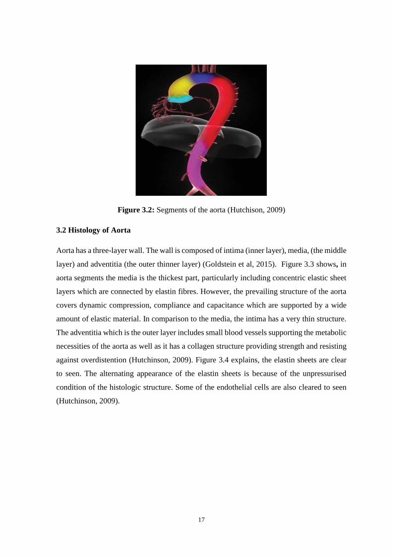
Figure 3.2 shows, the abdominal aorta (pink), the descending aorta (red), the aortic arch
(dark blue), the ascending aorta (yellow), the aortic root (light blue), the sinotubular junction
(green) (Hutchison, 2009).
Pars descendens aortae
[Aorta descendens]
Pars ascendens aortae
[Aorta ascendens]
17
Figure 3.2: Segments of the aorta (Hutchison, 2009)
3.2 Histology of Aorta
Aorta has a three-layer wall. The wall is composed of intima (inner layer), media, (the middle
layer) and adventitia (the outer thinner layer) (Goldstein et al, 2015). Figure 3.3 shows, in
aorta segments the media is the thickest part, particularly including concentric elastic sheet
layers which are connected by elastin fibres. However, the prevailing structure of the aorta
covers dynamic compression, compliance and capacitance which are supported by a wide
amount of elastic material. In comparison to the media, the intima has a very thin structure.
The adventitia which is the outer layer includes small blood vessels supporting the metabolic
necessities of the aorta as well as it has a collagen structure providing strength and resisting
against overdistention (Hutchinson, 2009). Figure 3.4 explains, the elastin sheets are clear
to seen. The alternating appearance of the elastin sheets is because of the unpressurised
condition of the histologic structure. Some of the endothelial cells are also cleared to seen
(Hutchinson, 2009).

18
Figure 3.3: Main Components of the aorta (Hutchinson, 2009)
Figure 3.4: Appearance of elastin sheets (Hutchinson, 2009)
3.2.1 The intima
The main structure of the intima includes the endothelial monolayer and the subendothelial
space. If the function is normal without any disease or trauma, the intima insists upon
thrombosis and atherosclerosis. It is generally get infected by several factors such as
smoking, diabetes, hypertension and dyslipidemia or traumatized and the intima starts to
spawn thrombi, ulcers and atherosclerotic plaques (Hutchinson, 2009).
3.2.2 The media
The main structure of the media includes elastic sheets formed by concentric layers bounded
to elastin fibrils and collagen sheets intervene with ground substance and various smooth
muscle cells. The structure of the aorta is known by the thickness of the media controlled
through layers of elastin sheets or lamellae (Hutchinson, 2009).

19
The media becomes poor due to hereditary disorders such as Marfan syndrome or bicuspid
aortic valve or diseased by a subsequent disorder like atherosclerosis or hypertension. It
becomes weak against overdistention that may cause an inability to get the stroke volume at
physiologic pressure occurring by systolic hypertension and an increase in the pulse wave
velocity. Moreover, dilation and poor functioning occur because of aneurysms, traumatic
cleavage within the layers, inducing intramural hematoma or dissection and increase in
atherosclerotic plaques causing intramural hematoma, rapture or penetration (Hutchinson,
2009).
3.2.3 The adventitia
The adventitia is the outer layer with a thin structure formed by vasa vasorum supplying
blood to the aorta and collagen. It is supportive against the metabolic necessities of the aorta
and stands as a last wall against rupture. In the existence of a disease, it supplies the
circulation of syphilitic treponemes. Moreover, if the number of vasa vasorum decreases in
the segments of aorta, the evolvement of atherosclerosis is highly possible (Hutchinson,
2009).
3. 3 Imaging Modalities of Aorta
The structure of the aorta is an elaborated geometrical shape and determining the shape as
well as the size requires various measurements. These measurements could be applied using
vertical angles to the axis of the aorta regarding to designate the diameter. The changes in
the size and shape of the aorta over time could be easily examined through constant
measurements and could reduce the possible errors is measures of arterial growth (Erbel et
al., 2014).
In order to avoid random possible error, attentive comparison of several measurements has
to be implemented preferentially with the same imaging methods. Using three-dimensional
CT scanning for measuring the exact aneurysm diameter, vertically to the centreline of the
vessel could give the best result. This technique gives an advantage of getting more certain
and producible correct measurements of the diameter of an aorta in comparison to axial
cross-section diameters especially in tortuous or kinked vessel in which the cranio-caudal
axis of the patient is not parallel to the vessel axis (Erbel et al., 2014).
20
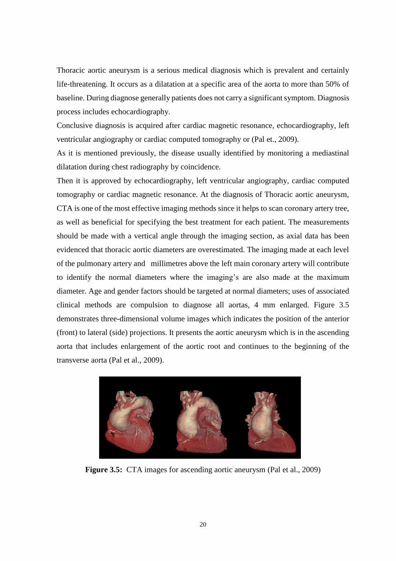
Thoracic aortic aneurysm is a serious medical diagnosis which is prevalent and certainly
life-threatening. It occurs as a dilatation at a specific area of the aorta to more than 50% of
baseline. During diagnose generally patients does not carry a significant symptom. Diagnosis
process includes echocardiography.
Conclusive diagnosis is acquired after cardiac magnetic resonance, echocardiography, left
ventricular angiography or cardiac computed tomography or (Pal et., 2009).
As it is mentioned previously, the disease usually identified by monitoring a mediastinal
dilatation during chest radiography by coincidence.
Then it is approved by echocardiography, left ventricular angiography, cardiac computed
tomography or cardiac magnetic resonance. At the diagnosis of Thoracic aortic aneurysm,
CTA is one of the most effective imaging methods since it helps to scan coronary artery tree,
as well as beneficial for specifying the best treatment for each patient. The measurements
should be made with a vertical angle through the imaging section, as axial data has been
evidenced that thoracic aortic diameters are overestimated. The imaging made at each level
of the pulmonary artery and millimetres above the left main coronary artery will contribute
to identify the normal diameters where the imaging’s are also made at the maximum
diameter. Age and gender factors should be targeted at normal diameters; uses of associated
clinical methods are compulsion to diagnose all aortas, 4 mm enlarged. Figure 3.5
demonstrates three-dimensional volume images which indicates the position of the anterior
(front) to lateral (side) projections. It presents the aortic aneurysm which is in the ascending
aorta that includes enlargement of the aortic root and continues to the beginning of the
transverse aorta (Pal et al., 2009).
Figure 3.5: CTA images for ascending aortic aneurysm (Pal et al., 2009)
21
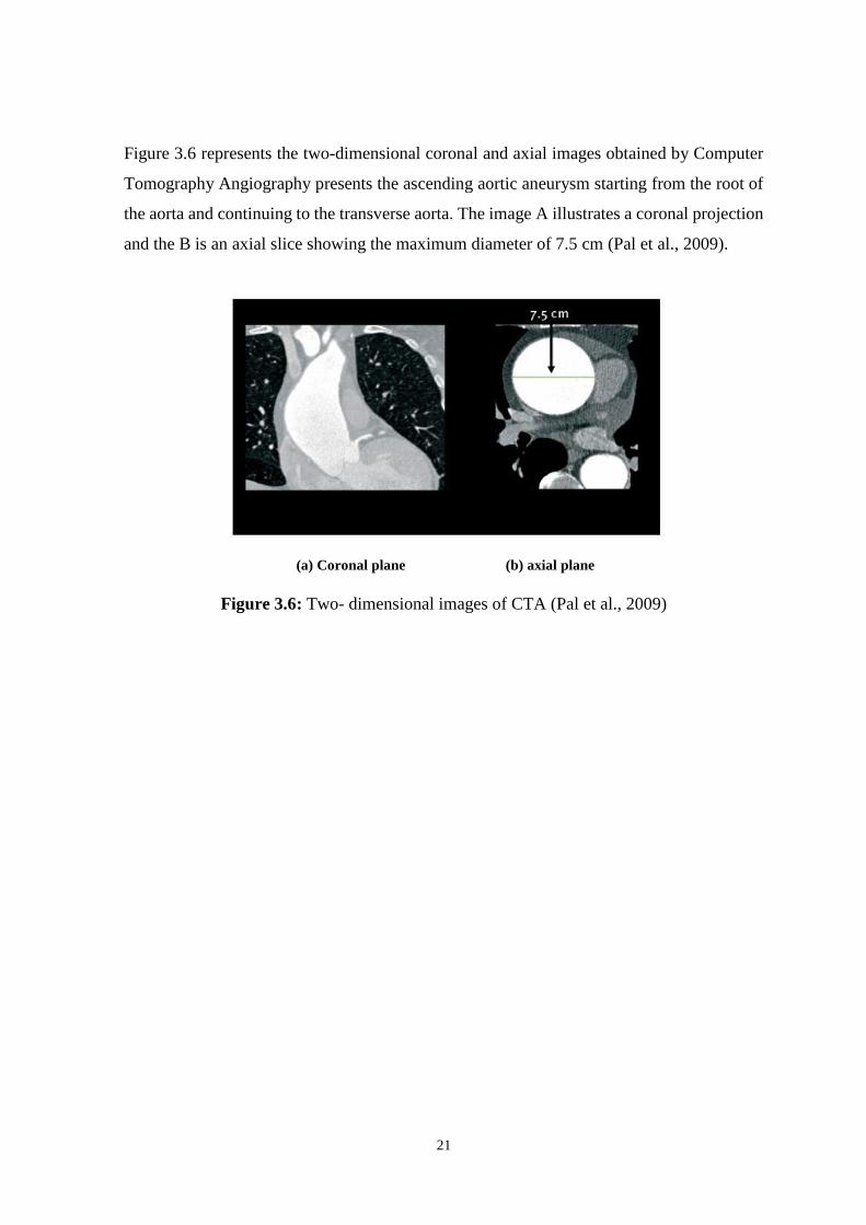
Figure 3.6 represents the two-dimensional coronal and axial images obtained by Computer
Tomography Angiography presents the ascending aortic aneurysm starting from the root of
the aorta and continuing to the transverse aorta. The image A illustrates a coronal projection
and the B is an axial slice showing the maximum diameter of 7.5 cm (Pal et al., 2009).
(a) Coronal plane (b) axial plane
Figure 3.6: Two- dimensional images of CTA (Pal et al., 2009)

22
CHAPTER 4
COMPUTER IMAGING AND DIGITAL IMAGE PROCESSING
4.1 Computer Imaging
The persistent innovations and improvements in technological equipment’s especially
computers have brought a lot of conveniences in every field of human life. The existence of
computers has contributed to practice different applications in different fields like
entertainment industry, health and insurance sectors as well as the internet which helps to
communicate with others easily, sending different data such as written documents visual
information and digital images.
Computer imaging is about gathering and processing visual information through computer.
Delivering information through images has a significant effect since the primary sense of
human being is visual and this method is known and used for centuries. By using images, it
is easier to deliver information compared to using thousands of words. In computer imaging,
huge amount of data is necessary for composing several subareas like compression and
image segmentation. Also, computer imaging creates certain top-level visual information to
receivers, human and as well as to the computers.
With this approach computer imaging can be used as two separate primary applications
which are computer vision and image processing. Analysis of images is used as primary data
in composing and arranging both applications. In computer vision, images are used by a
computer, where the images gained through images processing application are for people.
There are several limits and strengths on human visual and computer vision system where
the specialists should examine the different functions and processing of these two systems.
The process of image analysis includes the inspection of image data to sort out any
outstanding imaging problem. The methods of image analysis include the main contents of
a computer vision system which examines the images and computerise the results. So, a
computer vision application is a system which deploys images. Image analysis is vital in the
development of an image processing algorithm where images should be tested and examined
(Umbaugh, 2005).

23
4.2 Image Analysis and Computer Vision
Image analysis has several functions such as searching image data for different applications.
In general, this helps to examine raw image data more detailed, gather more information
about images and how images can be used efficiently to collect the necessary information
requested. The image analysis process is performed through various appliances such as
image segmentation, pattern classification, image transforms and feature extraction. Image
segmentation is used for distinguishing higher-level images between raw image data where
extraction carries out the process of collecting information of higher level images by shape
or colour. Feature extraction also supported by image transforms to extract dimensional
frequency information. Higher level information is carried out by pattern classification
which also designates objects within images (Umbaugh, 2005).
4.3 Image Processing
Image processing is utilised by using a special computer software system which is controlled
and directed by human. The images are carried and examined by people. The operation of
human visual system should be well understood for using these types of computer
applications. The main aspects covered by image processing are image compression,
restoration and enhancement. It is important to study how human visual perception reacts on
raw image data during the process of compressing, restoring or enhancing digital images.
Digital image is an image described as a two-dimensional function which is f (x, y), where
x and y are in a plane sequent and the extent of f at each sequent (x, y) and the vitality rates
of f are all limitless, with different quantities are called a digital image. The process of digital
image processing includes the formatting of images through a computer. A digital image is
formed by a finite number of components where each of them has a specific area and value.
These are pixels, pels, picture elements and image elements. Pixel can be described as the
components of a digital image. Images are the most specific and effective way of responding
human perception touching their senses. Imaging equipment’s include the whole
electromagnetic spectrum (EM) which differs from radio waves to gamma. The machines
help people to associate with images that are formed by other tools where human being are
not familiar. Some of these machines are electron microscopy, computer-generated images
24
and ultra-sound. However digital imaging process requires a huge amount of applications
with different fields (Gonzalez and Woods, 2002).
There are many significant and important image processing applications which are used by
medical community. Some of these include several series of diagnostic imaging. Diagnostic
imaging involves methods such as CT, MRI Scanning and PET which contributes medical
experts to examine human body without doing any surgical operation. These applications
covered by image processing are also used in different fields, for example for observing
microscopic images in biological researches. Also, entertainment sector uses image
processing for computer animations, special effects, and creating artificial scenes which are
all related to computer graphics. Image processing helps people to have an idea of how they
will be look like with a new pair of glasses, haircut or new lips. Designs made by computer
which are processed through several tools of image processing and personal computer
graphics contribute people to design a new car or house as well as explore the image either
by enlarging or reducing the size. These features of the applications could be used for
modifying interior area of a house, or building and help to see the outcome through computer
context.
Such applications that allow people to perform virtual workshops and executions are
continuously developing and by the improvements on image processing applications and
new technological innovations human life will be affected positively in many fields
(Umbaugh, 2005).
Moreover, areas like computer vision which aims the usage of computing in order to excel
human vision as well as understanding and inferring and performing on visual data. This
field is included in artificial intelligence (AI) where the target is to excel human
perceptiveness. Artificial intelligence is in its development process with the issue of the
performance which is actually lower than originally expected. The field that examines
images which also described as image understanding is in the middle the field of computer
vision and image processing. There are no certain connections in the continuum from image
processing at one end to computer vision at the other. However, another example is to pay
attention that there are three kinds of computerized processes within this continuum which
are low-mid, mid-level and high-level processes. Low-level processes include initial
processes like image pre-processing in order to decrease contrast, noise, sharpening and
enhancement. A low-level process is featured where both its inputs and outputs are formed

25
by images. Mid-level processing includes several duties like division of an image into
segments, description of these segments to decrease their amount for creating computer
processing, and classification of each segments. A mid-level process is featured by its inputs
which are usually images, however outputs are connections evaluated from those images
such as contours and edges. Lastly, higher level processing covers making sense of a
collection of selected objects, as an examination and at the last phase of continuum practicing
the comprehensive task which are normally related to the vision (Gonzalez and Woods,
2002).
4.4 Computer Imaging Systems
Computer imaging systems could vary and differ according to the applications used. Every
day depending on technological improvements, these systems are getting more efficient in
terms of speed, usage and processing. There are two main component types of computer
imaging systems which are software and hardware. The computer, display tools and the
image acquisition subsystem are categorised as hardware components.
However, software components contribute to transform or formatting images, carry out
necessary analysis and functioning image data. Moreover, it is used for controlling image
collection and process of storage.
The term digitization is used for converting a simple video signal into a digital image. Since
a simple video signal is in an analogue form, digitization is necessary where the computer
needs a sampled version of the video signal. A significant video signal includes video
information frames which connect with the full screen of visual information. These frames
may split into a number of parts and each part forms consecutive video information lines.
The image data could be acquired in a two-dimensional form where every single data is
proposed to as a pixel. The following notation will be used for digital images, I (r, c) = the
brightness of the image at the point (r, c).

26
Figure 4.1: The hierarchical image pyramid (Umbaugh, 2005)
After getting the data in digital form the software is used for processing the data. The
illustration of this processing is made by the hierarchical image pyramid used in Figure 4.1.
At the bottom level, individual pixels are processed where low level performing may be
carried out. The second level of the pyramid is the neighbourhood that includes a single pixel
and the surrounding pixel where pre-processing operations could take place in this level. The
higher level of image representation is made at the top level of the hierarchical pyramid
where there are fewer amounts of data (Umbaugh, 2005).
4.5 Image Formatting and Sensing
A device with energy interaction which allows people to carry out several measurements is
used to form digital images. These measurements are necessary in various fields across a
two-dimensional grid in the world for creating images. The devices used for these
measurements are called sensors. Sensors have features of responding to many significant
types of electromagnetic (EM) spectrum, lasers, electron beams, sound energy and any type
of signals that could be measured.
The EM spectrum is made up of infrared, visible light, x-rays, ultraviolet, radio waves,
gamma waves or microwaves. Electromagnetic radiation includes variable electric and
magnetic ranges which are vertical to each other and deploy continuously.

27
These waves move with a light speed in free space, roughly 3x10⁸ meters/second (m/s) and
are categorized according to their wavelength and frequency. The name of the bands in EM
spectrum depends to the history of discovery reasons or the way they are applied. Beside
this, EM radiation can be illustrated as a stream of massless particles which are called
photons. Photons comply with the quantum which is the minimum amount of energy that
could be measured through EM signal. Electron volts help to measure the energy of photon.
Electron volts are very small units of kinetic energy which are used by electron to accelerate
through an electronic capacity of one volt. EM shows that the increase in the frequency raises
the energy within the photon. Since the smallest frequencies are in radio waves it is safer to
be used where gamma rays are very dangerous because of consisting highest energy.
Imaging process with gamma rays performed through measuring the rays spread from the
object (Umbaugh, 2005).
4.6 Imaging Outside the Visible Range of the EM Spectrum
Positron emission tomography (PET) in nuclear medicine is performed by injecting
radioactive isotope to a patient; while it breaks gamma-rays are perceived and measured. In
medical diagnostic x-rays are used by a film which responds to x-ray energy established
between the energy source and the patient. Moreover, x-rays are used in computerized
tomography (CT), where a detector surrounds patient and operated to receive two-
dimensional slices which can be converted into three-dimensional image. Fluorescence
microscopy is done by dyes which spread visible light while ultraviolet light (UV) is
dispersed.
Figure 4.2 illustrates, X-ray and UV images: (a) X-ray of a chest with an implanted electronic
device to endorse the heart. (Image courtesy of George Dean.) (b) Dental x-ray. (c) and (d)
Cells imaged by fluorescence microscopy, performed by using visible light while ultraviolet
light was used for illumination. (Cell images courtesy of Sara Sawyer, SIUE.) (e) Patient’s
abdomen imaged by computerized tomography (CT) several 2-D images were obtained
through different angles and were accumulated for converting a 3-D image (Image courtesy
of George Dean.) (Umbaugh, 2005).

28
(a) X-ray chest image (b) Dental x-ray image
(c) Cell images (d) Cell images
(e) CT abdomen image
Figure 4.2: X-ray and UV images (Umbaugh, 2005)
Magnetic Resonance Imaging (MRI) used in medicine is done by sending radio waves to
patient’s body with short pulses through a powerful magnetic tool. Patient’s body shows a
reaction to each pulse and spreads radio waves. These radio waves are measured by the tool
to from an image of the specific body parts of the patient. There is a special antenna (receiver
coil) of MRI systems which perceives this interactivity between radio-frequency EM and
atomic nuclei in the body of the patient. There are also superconducting magnets in MRI
systems which forms fields with magnitudes from 0.1 to 3.0 Tesla (1,000 TO 30,000 Gauss)
The contrast resolution of MRI systems is efficient where they highly contribute to view
inconspicuous differences between organs and the soft tissues which could not be visualized
easily by using CT films or x-ray (Umbaugh, 2005). Figure 4.3 demonstrates the images of
multispectral and radio wave. (a) Multispectral Geostationary Environment Satellite (GOES)
image of North America, showing a large tropical storm off Baja California, a frontal system

29
over the Midwest, and tropical storm Diana off the east coast of Florida. (Courtesy of
NOAA) (b) Magnetic resonance image (MRI) of a patient’s shoulder. MRI images are
created using radio waves.
This is a single 2-D slice; various images are obtained through different angles and were
accumulated for converting a 3-D image. Image courtesy of George Dean.) (Umbaugh,
2005).
(a) GOES image of North America (b) MRI shoulder image
Figure 4.3: Multispectral and radio wave images (Umbaugh, 2005)
4.7 Image Representation
As discussed previously, imaging sensors operates by detecting image as a batch of
outspread light energy which forms an optical image. These types of images are seen in
everyday life, captured by cameras, displayed through device monitors. While analog
electrical signals are formed, these optical images are designated as video information and
used as pattern to create digital image I (r, c), where I represents digital image and r and c
represents row and column coordinates respectively.
The digital image which is called I (r, c), it is created by two-dimensional array of
information which every single pixel conforms to the illumination of the image at the point
(r, c). The image model used here which is two-dimensional array I (r, c) is considered as a
matrix and one column is named as a vector in linear algebra terms. The image data of this
model is one-colour, gray-scale which could be described as monochrome. However, there
are various types of image data which needed to be extended and modified for this model.
Frequently, these image data are multi-band images in terms of multispectral or colour,

30
which can be sampled by I (r, c) function conforming to every single information received
by the band of brightness. The images evaluated here are, multispectral, colour, binary and
gray-scale (Umbaugh, 2005).
4.7.1 Binary images
Binary images are the easiest form of images which generally includes two values, 0 and 1
or black and white. A binary image stands for 1-bit per image pixel where 1 binary digit
represents each pixel. Generally, these images are used in such applications of computer
visual where the only data needed is for outlining, information and general shape within the
task.
Threshold operation where each pixel above the value of threshold turn 1 and value below
are black contributes gray-scale images to form binary images. Despite, this process induces
losing information, the image file gained is much smaller which helps to transmit and store
the data easily.
4.7.2 Gray-scale images
Gray-scale images are one colour images which are called monochrome. There is no colour
information, only brightness information is consisted. Different brightness levels are
designated by the number of bits used for each pixel.
A simple gray-scale image includes 8-bit per pixel data which helps to gain various
brightness levels between 0-255. Regarding to human visual system’s features, this
representation gives more efficient resolution of brightness and provides a noise margin
through giving much more gray levels than expected. The noise margin is the false
information in the signal which is efficient in receiving different types of noise included
within the real systems structure. Moreover, in digital computers the standard small unit of
data is byte which corresponds to 8-bits of data in this representation.
4.7.3 Colour images
Colour images might be described as three-band monochrome where each data band pertains
to a particular colour. The real data gained through the digital image is the information of
brightness formed in every single spectral band. While the image is showed, the pertained
brightness data comes up on the screen through picture elements which spread light energy
31
relying on each colour. The basic colours of images are RGB images, green, blue and red.
Compared to the 8-bit monochrome model, corresponding colour image should be 24-bits
per pixel where it includes 8-bits for each colour red, green and blue in colour band.
In many applications, RGB colour information is converted into a mathematical space which
evaluates the colour information from the brightness information. This process is named as
a colour transform, a colour model, or matching with another colour space. After the process
is completed, the image information creates one-dimensional illumination, two-dimensional
colour space, space or luminance. There is no brightness information included within two-
dimensional colour space. However, it includes information depending on the engaged
mounts of the different colours. In this sense, another advantage of modelling the colour
information is creation of more people-oriented methods of identifying particular colours.
4.7.4 Multispectral Images
Multispectral images generally include information outside the normal human
comprehension range. These ranges contain ultraviolet, infrared, x-ray and other bands in
the EM spectrum. These could not be estimated as images where the information described
could not be visualised directly by human. However, by matching different spectral bands
to RGB components, information could be visualized. If there are more than three bands of
information within multispectral image, the dimension is decreased in order to view image
by using the main components of transform.
4.8 Digital images file formats
Since there are many types of images and applications with particular requirements digital
image file formatting is necessary. There are several standard types of file formatting exists
and the formats used here are generally in use.
A field of computer graphics are directly related to computer imaging. Computer graphics is
about reproduction of visual data by using computer which is a specialized field in computer
science. The reproduction process includes manipulation and generation of any type of
images as well as to display or print through fixing devices such as camera, monitor or printer
to a pc which provides images.
There are two main categories image data in computer graphics; vector and bitmap. Bitmap
images which are also named as raster images can be extended by the model I (r, c) where

32
there is pixel information and values of corresponding illumination kept in several file
formats. Vector images consists the procedures of curves, presenting lines and patterns by
saving the main points. These main points are necessary for defining the shapes and the
method of converting these into an image which is called rendering. This process forms
bitmap format where every single pixel has significant values related with it.
Many of the file formats explained above are in the field of bitmap images; however, some
of the formats are compressed. So, if the file is not decompressed, the I (r, c) values could
not be directly available. Generally, these images include the information of the pixel data
and the header. The image file header includes several parameters occur at the beginning of
the file and specific information such as number of rows, columns, bands, bits per pixel and
the file types should be included. Moreover, certain types of file formats could be complex
where the header may include information of compress applied and other parameters used
in creation of the image I (r, c).
The Microsoft Windows bitmap format is more widely used by computers operating under
Windows. So, imaging and graphics applications used under Windows processing system
support BMP format. The format includes elementary headers followed by the raw image
data and it is simply operating. The other most common format used is JPEG, Joint
Photographic Experts Group, compressing high number of images, mostly used on the
Internet to decrease the bandwidth and reduces the time of viewing an image (Umbaugh,
2005).
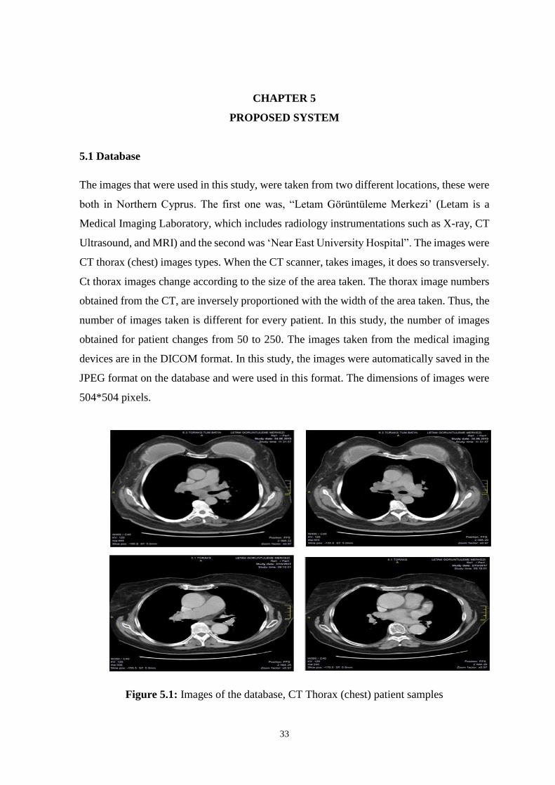
33
CHAPTER 5
PROPOSED SYSTEM
5.1 Database
The images that were used in this study, were taken from two different locations, these were
both in Northern Cyprus. The first one was, “Letam Görüntüleme Merkezi’ (Letam is a
Medical Imaging Laboratory, which includes radiology instrumentations such as X-ray, CT
Ultrasound, and MRI) and the second was ‘Near East University Hospital”. The images were
CT thorax (chest) images types. When the CT scanner, takes images, it does so transversely.
Ct thorax images change according to the size of the area taken. The thorax image numbers
obtained from the CT, are inversely proportioned with the width of the area taken. Thus, the
number of images taken is different for every patient. In this study, the number of images
obtained for patient changes from 50 to 250. The images taken from the medical imaging
devices are in the DICOM format. In this study, the images were automatically saved in the
JPEG format on the database and were used in this format. The dimensions of images were
504*504 pixels.
Figure 5.1: Images of the database, CT Thorax (chest) patient samples

34
5.2 Proposed System
A block diagram representation of the steps used in the proposed system is shown in Figure
5.2.
Figure 5.2: Block diagram of the proposed system

35
5.2.1 Image Binarization (Thresholding)
Thresholding is an image segmentation method, it is a very simple method and commonly
used. The objective of thresholding is to cause segmentation of an image into different parts
which have different interest values and to take away other areas that are not necessary.
In simplest thresholding technique, a single threshold is used to separate objects and value
anything of interest.
However, at other times the single threshold technique does not provide a correct
segmentation result for the entire image. In these cases, other threshold techniques are used,
these include variable threshold and multilevel threshold techniques, all of them are based
on measurements from various statistics. (Ritter and Wilson, 2000).
Normally a gray level image is used to create a binary image, to do this a threshold operation
must be applied. In order to do this, a threshold value must be specified. In this process, all
values will be set above the specified gray level to ‘1’, all other values must be below the
value of ‘0’. In fact, the value for ‘0’ and ‘1’ can be anything, so if you have the number 255
for this number you have to use ‘1’ and for 0 you use the value ‘0’. In using this threshold
method, the values will be sought by trial and error, and this will rely on lighting and other
objects surrounding the item in contrast to it. The best way to find an acceptable threshold
value is with good lighting and good contrast between the objects and all the background
imagery (Umbaugh,2005).
The threshold image g (x, y) can be described as
𝑔(𝑥, 𝑦) = {1 𝑖𝑓 𝑓(𝑥, 𝑦) > 𝑇
0 𝑖𝑓 𝑓(𝑥, 𝑦) ≤ 𝑇 (5.1)
Pixels labeled 1, they normally correspond to object and to convenient gray level pixels
labeled 0 correspond to the background or any other gray level not assigned to any other
objects. Whereas T depends only on f (x, y) (for gray-level values) the threshold is defined
as global (Gonzalez and Woods, 2002).
The global thresholding method is applied for remove objects of interest having values
different from the background (Ritter and Wilson, 2000).
In this study, the threshold value that determines number of pixels to be segmented was
chosen by trial and error.

36
In order to cause a better resolution in the images, several values had been tried and three of
them which caused a different degree of illumination in contrast to the background of the
images, were determined to be used. The program runs three levels of threshold values prior
to the circle detection. In this study, RGB images were used and converted into a binary
image, by using the binarization (thresholding) method. Figure 5.3, shows, how the
binarization method converts RGB images to Binary images.
(a) Original image (b) After image binarization
(c) Original image (d) After image binarization
Figure 5.3: Examples of the CT thorax images for the first test patient

37
5.2.2 Circular Hough transform
Circular Hough Transform (CHT) is used to investigate images in order to find circles, in
this process there is usually a strong noise present, and because this technique is very
effective that is the reason why this method is used, in the presence of occlusion and its
varying illumination.
CHT is not a very strong algorithm method, but because of the number of alternative
approaches which can be used and because there are three (3) main steps that is common to
all three.
1- Accumulator Array Computation.
The pixels from the foreground of high gradients are designed as a candidate pixel, which
then gives them the right to give votes in the accumulator array. In a classical CHT usage,
the candidate pixels vote in turn they form patterns these votes into a full circle by its
specified radius. Figure 5.4 (a) illustrates an example of candidate pixels which are lying on
an actual circle (solid circle) and the perfect CHT voting pattern (dashed circle) for the
candidate pixel (Mathworks).
Figure 5.4: Classical CHT voting pattern (Mathworks)

38
(5.3)
2- Center Estimation
As the candidate pixels give their votes, which are part of a circle which then comes together
as the accumulator array bin, which is relevant to the circles center. Thus, this means that
the circles center is then evaluated by calculating the peaks in the accumulator array.
Figure 5.4 (b) demonstrates an example of the candidate pixels (solid dots) which is on top
of an actual circle (solid circle) which shows their voting patterns (dashed circles) that concur
at the centre of the actual circle.
3- Radius Estimation
When you use the same accumulator array in more than one radius estimation, as it is done
regularly in the CHT algorithm, the radius of that circle has to be re-valuated as an alternative
step. (Mathworks)
When you are dealing with a circle, the equation of a circle becomes such as the following,
where a and b are the centre coordinates of the circle and d is the diameter (Umbaugh,2005).
(𝑟 − 𝑎)2 + (𝑐 − 𝑏)2 = (𝑑/2)2
In this work, after applying the image binarization, the Circular Hough Transform method
was used to automatically detect and calculate the radius of the patients’ aorta. After the
aorta is detected, the x, y coordinates of the aortas centre point are found and the aortas
radius was calculated. Then the diameter was determined by multiplying the radius by 2.
This is the widest point of the aorta that the radiologist needs to detect. The top aorta in the
patients’ image is the ascending aorta and the bottom one is called the descending (thoracic)
aorta. The program determines the aortas location by using the centre value of y coordinate
as its reference. In cases where patients do not have a fully circular formation of an aorta,
the measurements (manual and automated) may show differences. Better results can be
obtained for these patients by increasing the sensitivity value in the Circular Hough
Transform accumulator.
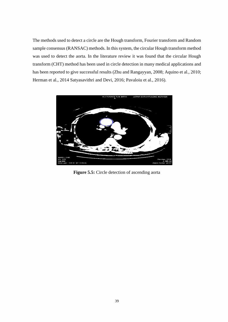
39
The methods used to detect a circle are the Hough transform, Fourier transform and Random
sample consensus (RANSAC) methods. In this system, the circular Hough transform method
was used to detect the aorta. In the literature review it was found that the circular Hough
transform (CHT) method has been used in circle detection in many medical applications and
has been reported to give successful results (Zhu and Rangayyan, 2008; Aquino et al., 2010;
Herman et al., 2014 Satyasavithri and Devi, 2016; Pavaloiu et al., 2016).
Figure 5.5: Circle detection of ascending aorta

40
5.2.3 Pixel to mm conversion factor for the image
In the images used in this work, there are 504 pixels from left to right and 504 pixels from
top to bottom resulting in 504x504 pixels in total. The pixel numbers can be seen on the
bottom left corner of Figure 5.7 (the first number shows the x axis from left to right and the
second number shows the y axis from top to bottom).
A yellow ruler line can be seen on the middle right of the image. Every step on this ruler is
1 cm. Thus, the ruler can measure up to 4cm of length. When looking at the first test patients
image, the y coordinate number on the yellow ruler is shown as 221, when looked at the ruler
line below it reads 234 pixels. Thus each 1 centimetres (cm) is equivalent to 234-221=13
pixels. As 1cm is equal to 10mm, then 1mm will be equal to 1.3 pixels.
Each image has a unique pixel value when converted to millimetres. In the patient images
taken, there is not a standard value that can be used to convert millimetres to pixels.
The ascending aorta diameter values have been automatically converted into mm by the
system. These steps are taken in this order; cropping, binarization (thresholding), edge
detection, Hough transform for line detection and Hough transform peak detection. The
reason for this process is because radiologists need to see the aorta diameter values in mm
or cm.
Figure 5.6: Ruler and Pixel Information in CT Scans

41
Cropping
In this work, for the pixel values to be converted into mm, the yellow ruler (4cm) on the
right of the patients’ images must be cropped and the scale is separated from the original
image. The coordinates values of yellow ruler are (470,210) and (495,280) for each image.
Figure 5.7: Cropping of Region of Interest
Then, cropped part of the image (4 cm scale) was converted into a binary image by using a
threshold value followed by edge detection.
Figure 5.8: Binarization (4 cm scale)

42
Edge detection
The edge detection method is one of the most commonly used image processing techniques
of medical imaging research. Medical images are made up of object edges and noise so it is
hard to tell the difference between the exact edge and the noise.
For feature extraction and feature detection the edge detection technique is essential. The
edges are formed of changes of concentration in an image (Goswami and Misra 2016).
Sobel Operator, is a system of edge detection method by which we can estimate the gradient
of the curve by a row and a column mask that will evaluate the first derivative on each side
of the graph.
Table 5.1: Edge detectors available in function Edge (Gonzalez et al., 2004)
Edge Detector
Basic Properties
Sobel Uses Sobel approximation
Prewitt Uses Prewitt approximation
Roberts Uses Roberts approximation
Laplacian of a Gaussian Zero crossing after Gaussian filtering f (x, y)
Zero crossings Zero crossing after a user specified filtering f (x, y)
Canny Finding local maxima of gradient of f (x, y)
Sobel Edge, detection mask constantly searches both up and down (vertically), also searches
sideways (horizontally), then it is able to combine this data into a single mathematical value
(Umbaugh,2005).
The masks can be described as:
|−1 −2 −1 0 0 0 1 2 1
| |−1 0 1−2 0 2−1 0 1
|
(a) Vertical Edge (b) Horizontal Edge
Figure 5.9: Sobel Masks (Umbaugh,2005)
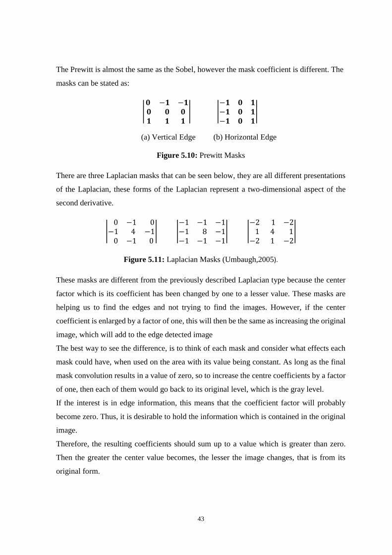
43
The Prewitt is almost the same as the Sobel, however the mask coefficient is different. The
masks can be stated as:
|𝟎 −𝟏 −𝟏 𝟎 𝟎 𝟎 𝟏 𝟏 𝟏
| |−𝟏 𝟎 𝟏−𝟏 𝟎 𝟏−𝟏 𝟎 𝟏
|
(a) Vertical Edge (b) Horizontal Edge
Figure 5.10: Prewitt Masks
There are three Laplacian masks that can be seen below, they are all different presentations
of the Laplacian, these forms of the Laplacian represent a two-dimensional aspect of the
second derivative.
| 0 −1 0−1 4 −1 0 −1 0
| |−1 −1 −1−1 8 −1−1 −1 −1
| |−2 1 −2 1 4 1−2 1 −2
|
Figure 5.11: Laplacian Masks (Umbaugh,2005).
These masks are different from the previously described Laplacian type because the center
factor which is its coefficient has been changed by one to a lesser value. These masks are
helping us to find the edges and not trying to find the images. However, if the center
coefficient is enlarged by a factor of one, this will then be the same as increasing the original
image, which will add to the edge detected image
The best way to see the difference, is to think of each mask and consider what effects each
mask could have, when used on the area with its value being constant. As long as the final
mask convolution results in a value of zero, so to increase the centre coefficients by a factor
of one, then each of them would go back to its original level, which is the gray level.
If the interest is in edge information, this means that the coefficient factor will probably
become zero. Thus, it is desirable to hold the information which is contained in the original
image.
Therefore, the resulting coefficients should sum up to a value which is greater than zero.
Then the greater the center value becomes, the lesser the image changes, that is from its
original form.

44
Another way of thinking about it, is that in extreme cases if the center coefficient becomes
very big, in comparison to the other coefficients in the mask.
The value of the pixels will be determined by their current value; however, the surrounding
pixels will only have a minimal effect upon them (Umbaugh,2005).
In this work, the commonly used Sobel, Prewitt, Roberts, Canny and Laplacian edge
detection techniques were used on the line found on the cropped images. Out of these
methods, the best results were obtained from the Prewitt operator. The line that was cropped
with the Prewitt operator method, provided the cleanest line, and its edges were easily
detected.
Figure 5.12: Prewitt operator Method (4cm scale)
Hough transform (line detection)
The way to find lines is by using the Hough transform method. This is a collection of edge
points which are used to determine a line. These edge points are usually adjacent to each
other and are usually in the same direction. The Hough transformation is an algorithm
technique which uses the collected edge points that were initially found by the edge detector
and uses an algorithm formula to plot all the points in a specifically patterned format and
this is how edge points are determined.
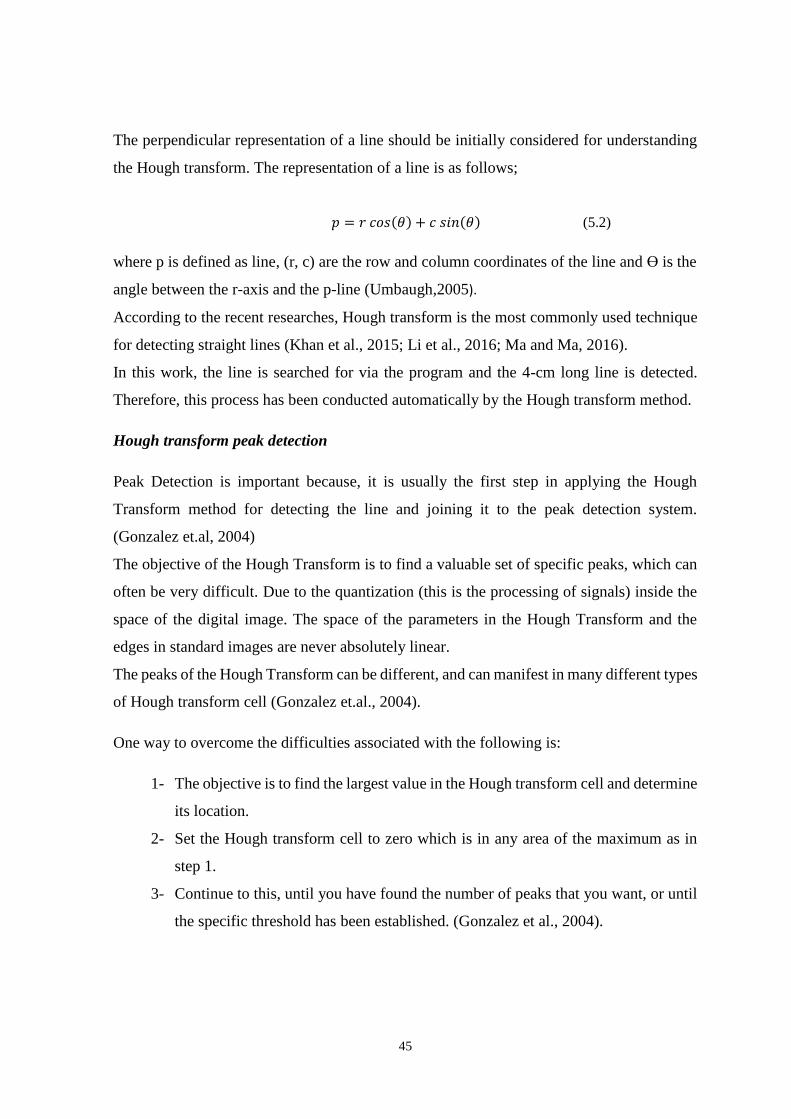
45
The perpendicular representation of a line should be initially considered for understanding
the Hough transform. The representation of a line is as follows;
𝑝 = 𝑟 𝑐𝑜𝑠(𝜃) + 𝑐 𝑠𝑖𝑛(𝜃) (5.2)
where p is defined as line, (r, c) are the row and column coordinates of the line and Ɵ is the
angle between the r-axis and the p-line (Umbaugh,2005).
According to the recent researches, Hough transform is the most commonly used technique
for detecting straight lines (Khan et al., 2015; Li et al., 2016; Ma and Ma, 2016).
In this work, the line is searched for via the program and the 4-cm long line is detected.
Therefore, this process has been conducted automatically by the Hough transform method.
Hough transform peak detection
Peak Detection is important because, it is usually the first step in applying the Hough
Transform method for detecting the line and joining it to the peak detection system.
(Gonzalez et.al, 2004)
The objective of the Hough Transform is to find a valuable set of specific peaks, which can
often be very difficult. Due to the quantization (this is the processing of signals) inside the
space of the digital image. The space of the parameters in the Hough Transform and the
edges in standard images are never absolutely linear.
The peaks of the Hough Transform can be different, and can manifest in many different types
of Hough transform cell (Gonzalez et.al., 2004).
One way to overcome the difficulties associated with the following is:
1- The objective is to find the largest value in the Hough transform cell and determine
its location.
2- Set the Hough transform cell to zero which is in any area of the maximum as in
step 1.
3- Continue to this, until you have found the number of peaks that you want, or until
the specific threshold has been established. (Gonzalez et al., 2004).

46
In this work, the peak points on the longest line (4cm-line) detected by the Hough transform
peak. Then the distance between two peak points was calculated in pixels. The calculated
distance value was converted to mm by dividing into 40 which is the conversion factor
(Conv) of the developed system.

47
CHAPTER 6
RESULTS AND DISCUSSION
6.1 Results
In this study, 20 patients CT thorax images were analysed using image processing
techniques. The ascending aorta diameter was automatically detected and measured via the
image processing techniques. The automatic and manual measurements were compared and
the difference was calculated as illustrated in the Table 6.1. The values measured
automatically by the program are close to those measured manually which is done by the
radiologist.
Table 6.1: Comparison of manually and automatically measured ascending aorta diameter
values and their difference
Manually measured
ascending aorta diameter
values by the radiologist
Automatically measured
ascending aorta diameter
values via the program
Difference
Patient 1 42.4 mm 43.1 mm 0.7 mm - 1.7 %
Patient 2 32.6 mm 32.0 mm 0.6 mm - 1.8 %
Patient 3 69.5 mm 70.0 mm 0.5 mm - 0.7 %
Patient 4 40.2 mm 38.0 mm 2.2 mm - 5.5 %
Patient 5 49.4 mm 49.7 mm 0.3 mm - 0.6 %
Patient 6 34.0 mm 34.3 mm 0.3 mm - 0.9 %
Patient 7 50.5 mm 49.8 mm 0.7 mm - 1.4%
Patient 8 33.8 mm 32.8 mm 1.0 mm - 3.0 %
Patient 9 31.7 mm 32.9 mm 1.2 mm - 3.8 %
Patient 10 34.0 mm 34.3 mm 0.3 mm - 0.9 %
Patient 11 32.0 mm 32.5 mm 0.5 mm - 1.6 %
Patient 12 48.3 mm 46.6 mm 1.7 mm - 3.5 %
Patient 13 38.1 mm 36.9 mm 1.2 mm - 3.1 %
Patient 14 42.4 mm 42.8 mm 0.4 mm - 0.9 %
Patient 15 29.0 mm 29.3 mm 0.3 mm - 1.0 %
Patient 16 36.8 mm 34.8 mm 2.0 mm - 5.4 %
Patient 17 41.5 mm 42.0 mm 0.5 mm - 1.2 %
Patient 18 27.9 mm 27.2 mm 0.7 mm - 2.5 %
Patient 19 50.4 mm 48.3 mm 2.1 mm - 4.2 %
Patient 20 37.6 mm 36.8 mm 0.8 mm - 2.1 %
Ave. = 0.9 mm - 2.3 %

48
There is an average of 2.3% and 0.9 mm difference between manual measurements and
automatic measurements. The % difference between these measurements was calculated
with the formula given in Equation 6.1.
% 𝑑𝑖𝑓𝑓𝑒𝑟𝑒𝑛𝑐𝑒 = |𝐴𝑢𝑡𝑜𝑚𝑎𝑡𝑖𝑐𝑎𝑙𝑙𝑦 𝑚𝑒𝑎𝑠𝑢𝑟𝑒𝑑 𝑣𝑎𝑙𝑢𝑒−𝑀𝑎𝑛𝑢𝑎𝑙𝑙𝑦 𝑚𝑒𝑎𝑠𝑢𝑟𝑒𝑑 𝑣𝑎𝑙𝑢𝑒
𝑀𝑎𝑛𝑢𝑎𝑙𝑙𝑦 𝑚𝑒𝑎𝑠𝑢𝑟𝑒𝑑 𝑣𝑎𝑙𝑢𝑒| 𝑋 100
The results for Patient 1 is shown in tabular form in Figure 6.1. It can be seen in the Figure
6.1 section (a), the program indicates detection of an ascending and descending aorta by
showing the word “YES “under column aorta. If ‘top’ is written in the aorta place, the
program shows the top image which is the ascending aorta and if ‘bottom’ is written it shows
the lower image which is the descending aorta. Figure 6.1 section (a), below shows 0.5 a
threshold value of the conversion of the RGB image into a binary image.
The ascending aortas diameter is measured in pixels by the program then automatically
converted to millimetres. The aorta diameter values measured by the program in pixels have
been automatically divided by the conversion factor (Conv) to be converted into mm. These
values show differences in each patient. Conversion factor represents that 1 mm is equal to
1.3 pixels for the images of the patient 1. The measured aorta diameters of patient 1 in all
images can be seen in Figure 6.2.
PATIENT 1
FILE AORTA PLACE DIAMETER(pixel) DIAMETER(mm) Conv
0.5
CT from I21.jpg YES TOP 54 41.5 1.3
CT from I22.jpg YES TOP 56 43.1 1.3
(a) Results of the program for patient 1
(6.1)

49
(b) Ascending aorta diameter value measured by the program (TH= 0.5)
(c) Ascending aorta diameter value measured by the program (TH= 0.5)

50
(d) Ascending aorta diameter values measured by the radiologist manually
Figure 6.1: CT Thorax images of patient 1
The number of images taken is different for every patient. The explanation of how many CT
scans are taken for each patient has been given. The 61 CT Thorax images of the patient
were searched by the program and the ascending aorta was automatically detected. The
ascending aortas diameter is measured by the program and the values are automatically
displayed in millimetres on the patient’s original image.
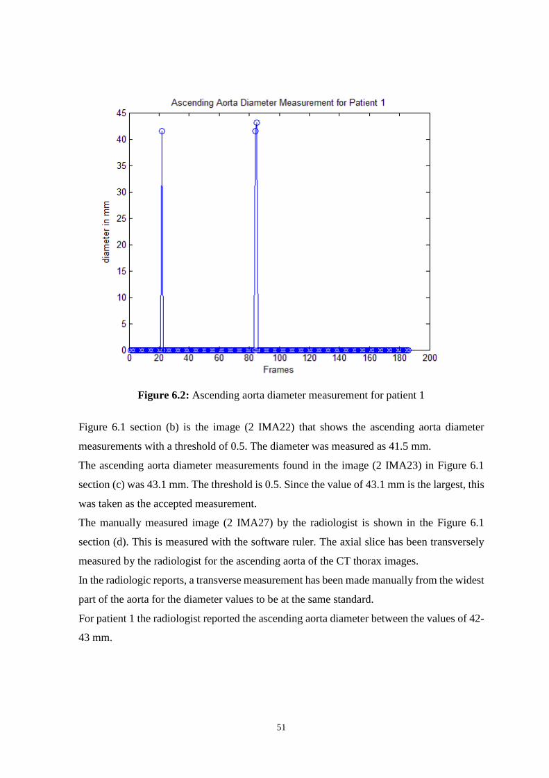
51
Figure 6.2: Ascending aorta diameter measurement for patient 1
Figure 6.1 section (b) is the image (2 IMA22) that shows the ascending aorta diameter
measurements with a threshold of 0.5. The diameter was measured as 41.5 mm.
The ascending aorta diameter measurements found in the image (2 IMA23) in Figure 6.1
section (c) was 43.1 mm. The threshold is 0.5. Since the value of 43.1 mm is the largest, this
was taken as the accepted measurement.
The manually measured image (2 IMA27) by the radiologist is shown in the Figure 6.1
section (d). This is measured with the software ruler. The axial slice has been transversely
measured by the radiologist for the ascending aorta of the CT thorax images.
In the radiologic reports, a transverse measurement has been made manually from the widest
part of the aorta for the diameter values to be at the same standard.
For patient 1 the radiologist reported the ascending aorta diameter between the values of 42-
43 mm.

52
The advantage of the program is that it automatically measures the widest values, due to
finding the centre point of the aorta, and gives a more sensitive and accurate measurement
when compared to the manual measurements done by the radiologist.
The ascending aorta diameter of this patient is greater than the normal limit because it is
more than 40 mm. This shows us that the patient ascending aorta is dilated. To prevent an
aneurysm from occurring, this patient must be closely controlled by the cardiologists.
The results for Patient 2 is shown in tabular form in Figure 6.2. The program indicates the
aorta place at the top in two images and at the bottom in two images in Figure 6.2 section
(a). The images found at the top are correctly ascending aortas. The two images where the
aorta is found at the bottom, measured the diameter of the bone instead of the diameter of
the aorta. This is an example of one of the mistakes that may form in the program however
this mistake can easily be determined and the risk can be prevented because the measured
image is shown to the user for them to verify the results. The radiologist can use the patients’
other images to obtain the correct aorta measurements.
PATIENT 2
FILE AORTA PLACE DIAMETER(pixel) DIAMETER(mm) Conv
0.5
CT from I29.jpg YES TOP 40 32 1.25
CT from I31.jpg YES TOP 40 32 1.25
0.6
CT from I44.jpg YES BOTTOM 40 32 1.25
CT from I64.jpg YES BOTTOM 56 44.8 1.25
(a) Results of the program for patient 2
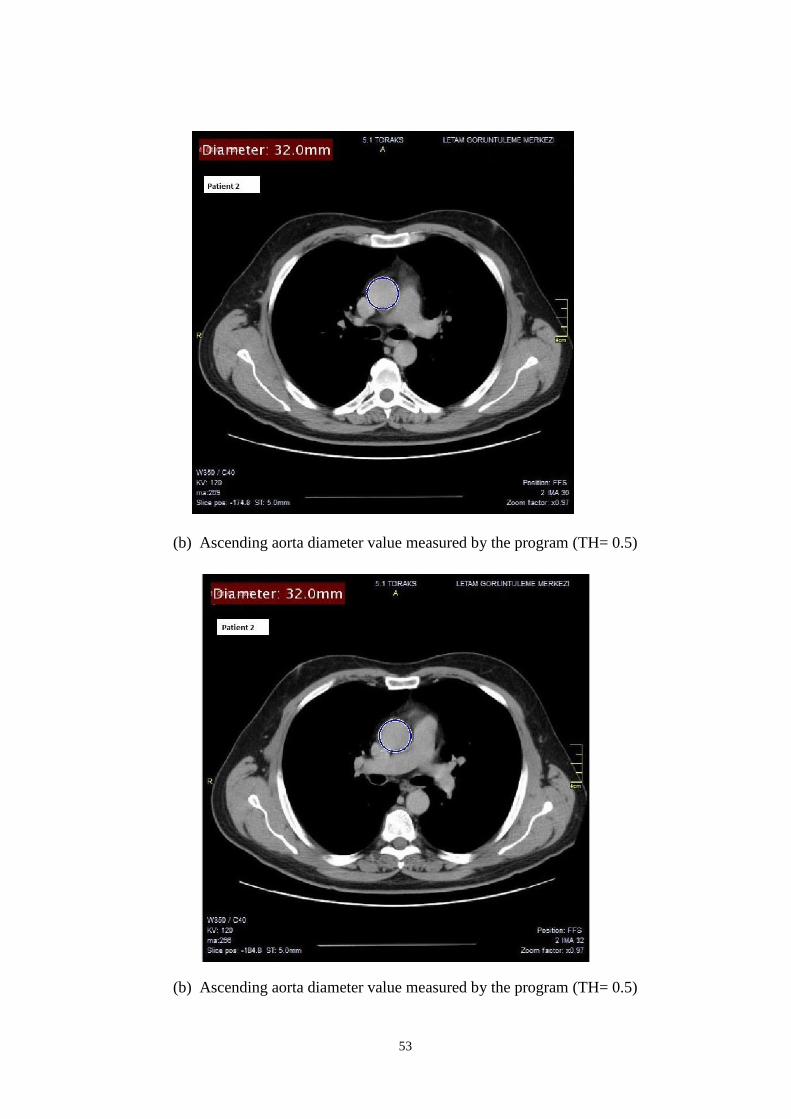
53
(b) Ascending aorta diameter value measured by the program (TH= 0.5)
(b) Ascending aorta diameter value measured by the program (TH= 0.5)
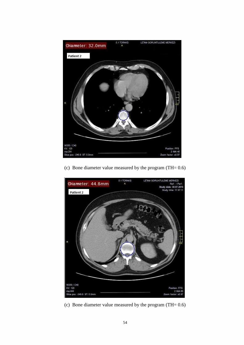
54
(c) Bone diameter value measured by the program (TH= 0.6)
(c) Bone diameter value measured by the program (TH= 0.6)
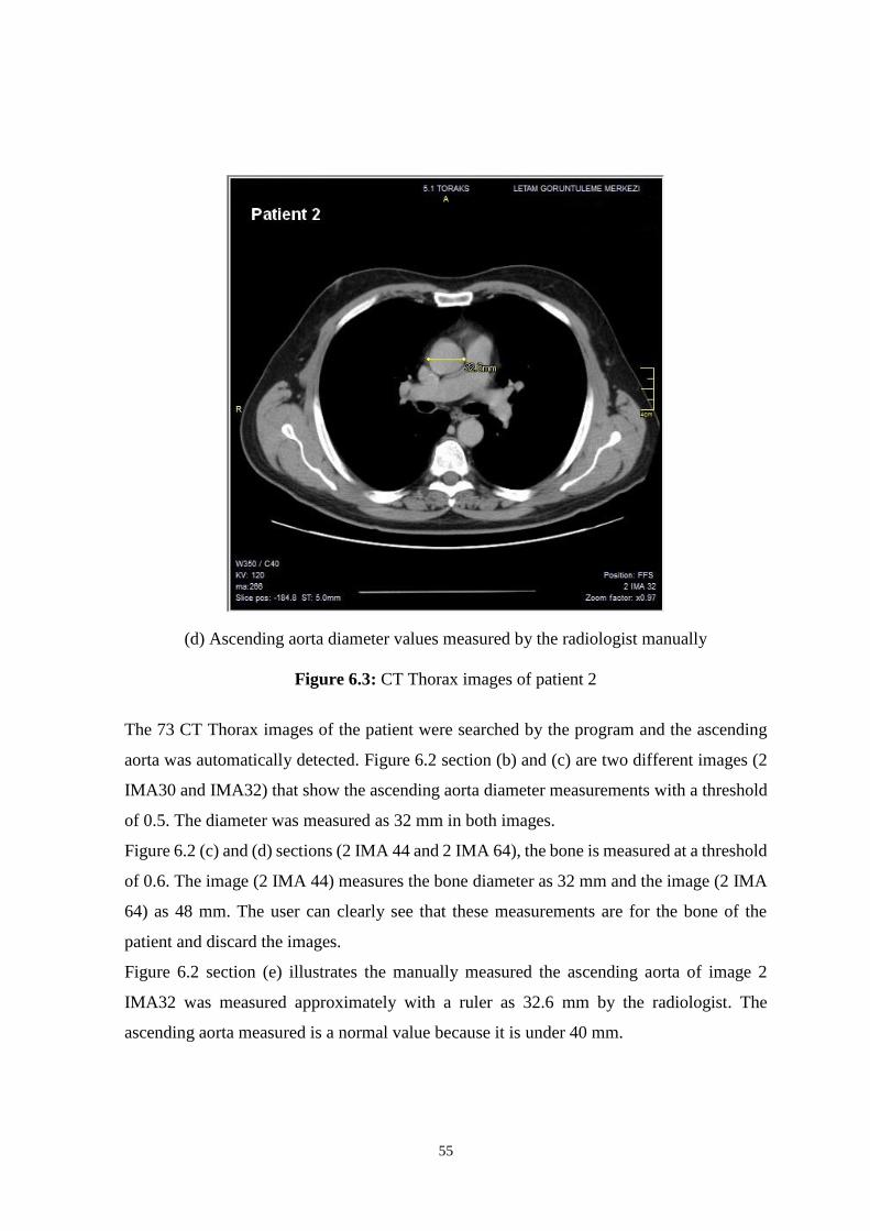
55
(d) Ascending aorta diameter values measured by the radiologist manually
Figure 6.3: CT Thorax images of patient 2
The 73 CT Thorax images of the patient were searched by the program and the ascending
aorta was automatically detected. Figure 6.2 section (b) and (c) are two different images (2
IMA30 and IMA32) that show the ascending aorta diameter measurements with a threshold
of 0.5. The diameter was measured as 32 mm in both images.
Figure 6.2 (c) and (d) sections (2 IMA 44 and 2 IMA 64), the bone is measured at a threshold
of 0.6. The image (2 IMA 44) measures the bone diameter as 32 mm and the image (2 IMA
64) as 48 mm. The user can clearly see that these measurements are for the bone of the
patient and discard the images.
Figure 6.2 section (e) illustrates the manually measured the ascending aorta of image 2
IMA32 was measured approximately with a ruler as 32.6 mm by the radiologist. The
ascending aorta measured is a normal value because it is under 40 mm.
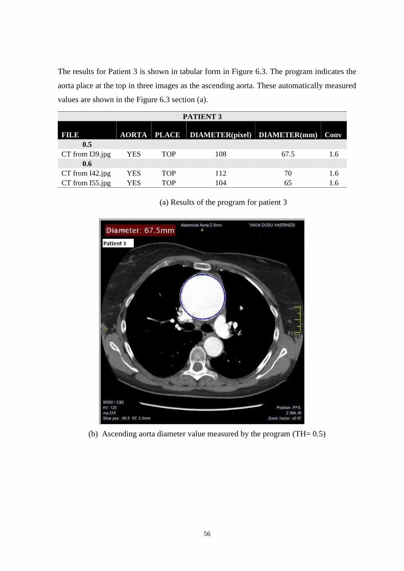
56
The results for Patient 3 is shown in tabular form in Figure 6.3. The program indicates the
aorta place at the top in three images as the ascending aorta. These automatically measured
values are shown in the Figure 6.3 section (a).
(a) Results of the program for patient 3
(b) Ascending aorta diameter value measured by the program (TH= 0.5)
PATIENT 3
FILE AORTA PLACE DIAMETER(pixel) DIAMETER(mm)
Conv
0.5 CT from I39.jpg YES TOP 108 67.5 1.6
0.6 CT from I42.jpg YES TOP 112 70 1.6
CT from I55.jpg YES TOP 104 65 1.6
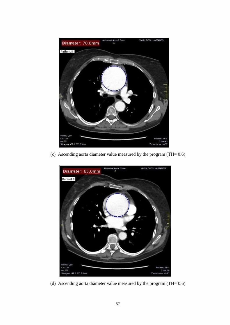
57
(c) Ascending aorta diameter value measured by the program (TH= 0.6)
(d) Ascending aorta diameter value measured by the program (TH= 0.6)

58
(e) Ascending aorta diameter values measured by the radiologist manually
Figure 6.4: CT Thorax images of patient 3
205 CT Thorax scans of the patient were searched by the program and the ascending aorta
was automatically detected.
The image 2 IMA40 that shows the ascending aorta diameter measurement with a threshold
of 0.5. The images 2 IMA 43 and 2 IMA 56 show the ascending aorta diameter measurements
with a threshold of 0.6. The diameter of image 2 IMA 40 was measured as 67.5 mm, 2 IMA
43 was measured as 70.0 mm and 2 IMA 56 was measured as 65.0 mm. Since the value of
70.0 mm is the largest, this was taken as the accepted measurement.
Figure 6.3 section (e) shows the radiologist measurement as 69.5 mm of image 2 IMA 46.
Due to this ascending aorta being above 50 mm, there is an aneurysm. Aneurysm increases
the risk of dissection and rupture. This has a life-threatening effect. This patient must
urgently be operated on by a heart surgeon because otherwise the patient may die of blood
loss.

59
6.2 Discussion
This proposed system is going to reduce the time it takes to evaluate the diameter of the aorta
when compared to manual measurements. It takes the radiologist some time to find the most
circular area in the images of the aorta and manually measure the largest diameter. The
radiologist does this measurement by eye ball estimation. Therefore, this system was
designed to mathematically find the most circular area of the aorta and measure the diameter,
thus reducing human errors.

60
CHAPTER 7
CONCLUSION AND SUGGESTIONS
7.1 Conclusion
Ascending aortic aneurysm is an enlargement of the ascending aorta. This disease has a life-
threatening effect. Because, it increases the risk of rupture in the patients ascending aorta
and it can cause loss of blood. From the literature review it is known that in the case of the
ascending aorta diameter being under 4 cm it is normal, between 4-5 cm dilated and above
5 cm has an aneurysm.
In this work, 20 patients Thorax (chest) CT scans were evaluated. The purpose of this work
is to automatically detect and measure the diameter of the ascending aorta from the Thorax
(chest) CT patient scans by the program. This system is not designed to replace doctors, but
to help, save time and increase accuracy.
In this work, a system is developed where most commonly used medical image processing
techniques are employed. Amongst these techniques firstly image binarization was used.
Then the circular Hough transform method was used to detect the ascending aorta and
measure its diameter in pixels. Lastly the Hough transform (line detection) method was used
to calculate the equivalence of pixels and millimetre on the CT thorax images.
Various problems were faced during this work. In some patient’s CT thorax scans, the
program recognised the bone within the circle and measured the bone diameter. These values
can be seen in the Figure 6.2 section (c) and (d). To solve this problem, the original patient
images are shown to the user to see whether or not the values found are bone measurements.
The radiologists have to choose the ascending aorta CT thorax images manually however,
the system developed in this study automatically choses the images that can be required by
the radiologists. Radiologists measure the diameter of the ascending aortas widest area
manually. When a patient is considered, different radiology specialist gives different
measurements. This is due to transverse measurements taken at the widest point. One
radiologist can measure different values each time. Thus, the aim of this system is to remove
these differences in measurement and obtain a reliable and definite result.
The principle advantage of this work is that it gives the same values each time. The manually
measured values and automatically measured values by the system of the ascending aorta

61
diameter are very close. An average of 2.3 % difference has been calculated between the
manual values and the values measured by the program. As, a difference of 2.3%
corresponds to the value of 0.9 mm, this percentage of difference is an acceptable value. The
acceptable difference rate for radiologists is approximately 2 mm.
7.2 Suggestions
For future work, the developed system can be made adaptable to the program of the medical
imaging devices used by doctors. It could be made to automatically measure the ascending
aorta diameter on the screen when the CT thorax scans are taken.
The sensitivity value in the program needs to be increased in some cases where the CT thorax
axial scans does not take the ascending aorta as fully circular. This must be increased
manually. The future work is the increment of this sensitivity automatically when the system
does not detect the ascending aorta.
Artificial Intelligence System can be used to evaluate whether or not the ascending aorta
diameter value is normal or if there is a problem such as dilation or an aneurysm.

62
REFERENCES
Adame, I. M., van der Geest, R. J., Bluemke, D. A., Lima, J. A., Reiber, J. H., & Lelieveldt,
B. P. (2006). Automatic vessel wall contour detection and quantification of wall
thickness in in-vivo MR images of the human aorta. Journal of Magnetic Resonance
Imaging, 24(3), 595-602.
Al-Agamy, A. O., Osman, N. F., & Fahmy, A. S. (2010, December). Segmentation of
ascending and descending aorta from magnetic resonance flow images. In Biomedical
Engineering Conference (CIBEC), 2010 5th Cairo International (pp. 41-44). IEEE.
American Heart Association. Aortic Aneurysm. Retrieved November 18, 2016 from
http://icardiomg.com/pdf/Aortic-Aneurysm.pdf.
Aquino, A., Gegúndez-Arias, M. E., & Marín, D. (2010). Detecting the optic disc boundary
in digital fundus images using morphological, edge detection, and feature extraction
techniques. IEEE transactions on medical imaging, 29(11), 1860-1869.
Avila-Montes, O. C., Kurkure, U., Nakazato, R., Berman, D. S., Dey, D., & Kakadiaris, I.
A. (2013). Segmentation of the thoracic aorta in noncontrast cardiac CT images. IEEE
journal of biomedical and health informatics, 17(5), 936-949.
Boxt, L., & Abbara, S. (2015). Cardiac Imaging: The Requisites. Elsevier Health Sciences.
Dehmeshki, J., Amin, H., Ebadian-Dehkordi, M., Jouannic, A., & Qanadli, S. (2009,
February). Computer aided detection and measurement of abdominal aortic aneurysm
using computed tomography digital images. In Digital Society, 2009. ICDS'09. Third
International Conference on (pp. 339-342). IEEE.
Entezari, P., Honarmand, A. R., Galizia, M. S., Yang, Y., Collins, J., Yaghmai, V., & Carr,
J. C. (2013). Analysis of the thoracic aorta using a semi-automated post processing
tool. European journal of radiology, 82(9), 1558-1564.
Erbel, R., Aboyans, V., Boileau, C., Bossone, E., Di Bartolomeo, R., Eggebrecht, H., ... &
Grabenwöger, M. (2014). 2014 ESC Guidelines on the diagnosis and treatment of
aortic diseases. European heart journal, 35(41), 2873-2926.

63
Fanelli, F., & Dake, M. D. (2009). Standard of practice for the endovascular treatment of
thoracic aortic aneurysms and type B dissections. Cardiovascular and interventional
radiology, 32(5), 849-860.
Frankel Cardiovascular Center University of Michigan Health System. Aortic Aneurysm.
Retrieved November 22, 2016 from http://www.umcvc.org/conditions-
treatments/aortic-aneurysm
Goldstein, S. A., Evangelista, A., Abbara, S., Arai, A., Asch, F. M., Badano, L. P., ... &
Devereux, R. B. (2015). Multimodality imaging of diseases of the thoracic aorta in
adults: from the American Society of Echocardiography and the European Association
of Cardiovascular Imaging: endorsed by the Society of Cardiovascular Computed
Tomography and Society for Cardiovascular Magnetic Resonance. Journal of the
American Society of Echocardiography, 28(2), 119-182.
Gonzalez, R., & Richard, E. (2002). C., and Woods, R., E., 2002. Digital image processing.
Gonzalez, R. C. E., Woods, S. L., Gonzalez, R. E. R. E. R. C., Woods, R. E., & Eddins, S.
L. (2004). Digital image processing using MATLAB (No. 04; TA1637, G6.).
Goswami, B., & Misra, S. K. (2016, March). Analysis of various Edge detection methods
for X-ray images. In Electrical, Electronics, and Optimization Techniques (ICEEOT),
International Conference on (pp. 2694-2699). IEEE.
Hermann, E., Bleicken, S., Subburaj, Y., & García-Sáez, A. J. (2014). Automated analysis
of giant unilamellar vesicles using circular Hough transformation. Bioinformatics,
30(12), 1747-1754.
Horikoshi, K., Hanaizumi, H., & Ishimaru, S. (2014, October). An automated recognition
technique for aorta aneurysm using thoracic multi-slice CT images. In Information
Theory and its Applications (ISITA), 2014 International Symposium on (pp. 65-69).
IEEE.
Hutchison, S. J. (2009). Aortic Diseases: Clinical Diagnostic Imaging Atlas. Elsevier Health
Sciences.
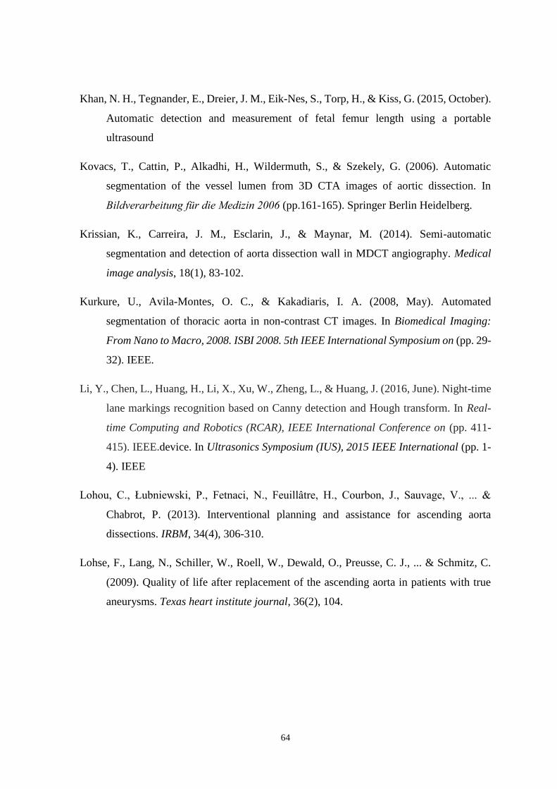
64
Khan, N. H., Tegnander, E., Dreier, J. M., Eik-Nes, S., Torp, H., & Kiss, G. (2015, October).
Automatic detection and measurement of fetal femur length using a portable
ultrasound
Kovacs, T., Cattin, P., Alkadhi, H., Wildermuth, S., & Szekely, G. (2006). Automatic
segmentation of the vessel lumen from 3D CTA images of aortic dissection. In
Bildverarbeitung für die Medizin 2006 (pp.161-165). Springer Berlin Heidelberg.
Krissian, K., Carreira, J. M., Esclarin, J., & Maynar, M. (2014). Semi-automatic
segmentation and detection of aorta dissection wall in MDCT angiography. Medical
image analysis, 18(1), 83-102.
Kurkure, U., Avila-Montes, O. C., & Kakadiaris, I. A. (2008, May). Automated
segmentation of thoracic aorta in non-contrast CT images. In Biomedical Imaging:
From Nano to Macro, 2008. ISBI 2008. 5th IEEE International Symposium on (pp. 29-
32). IEEE.
Li, Y., Chen, L., Huang, H., Li, X., Xu, W., Zheng, L., & Huang, J. (2016, June). Night-time
lane markings recognition based on Canny detection and Hough transform. In Real-
time Computing and Robotics (RCAR), IEEE International Conference on (pp. 411-
415). IEEE.device. In Ultrasonics Symposium (IUS), 2015 IEEE International (pp. 1-
4). IEEE
Lohou, C., Łubniewski, P., Fetnaci, N., Feuillâtre, H., Courbon, J., Sauvage, V., ... &
Chabrot, P. (2013). Interventional planning and assistance for ascending aorta
dissections. IRBM, 34(4), 306-310.
Lohse, F., Lang, N., Schiller, W., Roell, W., Dewald, O., Preusse, C. J., ... & Schmitz, C.
(2009). Quality of life after replacement of the ascending aorta in patients with true
aneurysms. Texas heart institute journal, 36(2), 104.

65
Lu, T. L. C., Rizzo, E., Marques-Vidal, P. M., von Segesser, L. K., Dehmeshki, J., &
Qanadli, S. D. (2010). Variability of ascending aorta diameter measurements as
assessed with electrocardiography-gated multidetector computerized tomography and
computer assisted diagnosis software. Interactive cardiovascular and thoracic
surgery, 10(2), 217-221.
Ma, T., & Ma, J. (2016, October). A sea-sky line detection method based on line segment
detector and Hough transform. In Computer and Communications (ICCC), 2016 2nd
IEEE International Conference on (pp. 700-703). IEEE.
Martínez-Mera, J. A., Tahoces, P. G., Carreira, J. M., Suárez-Cuenca, J. J., & Souto, M.
(2015). Automatic characterization of thoracic aortic aneurysms from CT images.
Computers in biology and medicine, 57, 74-83.
Mao, S. S., Ahmadi, N., Shah, B., Beckmann, D., Chen, A., Ngo, L., ... & Budoff, M. J.
(2008). Normal thoracic aorta diameter on cardiac computed tomography in healthy
asymptomatic adults: impact of age and gender. Academic radiology, 15(7), 827-834.
Mathworks. Find Circles Using Circular Hough Transform. Retrieved October 16, 2016
from https://www.mathworks.com/help/images/ref/imfindcircles.html
Mayo Clinic. Thoracic Aortic Aneurysm. Retrieved October 30, 2016 from
http://www.mayoclinic.org/diseases-conditions/thoracic-aortic-aneurysm/symptoms
causes/dxc-20122022.
Mirela-Maria, C., & Tiberiu, C. (2013). Aortic aneurysms and aortic dissection identification
using image segmentation with MATLAB. Universitatii Maritime Constanta. Analele,
14(20), 127.
Muraru, D., Maffessanti, F., Kocabay, G., Peluso, D., Dal Bianco, L., Piasentini, E., ... &
Badano, L. P. (2013). Ascending aorta diameters measured by echocardiography using
both leading edge-to-leading edge and inner edge-to-inner edge conventions in healthy
volunteers. European Heart Journal-Cardiovascular Imaging, jet173.
National Heart, Lung, and Blood Institute. Aneurysm. Retrieved October 30, 2016 from
https://www.ncbi.nlm.nih.gov/pubmedhealth/PMH0062939/
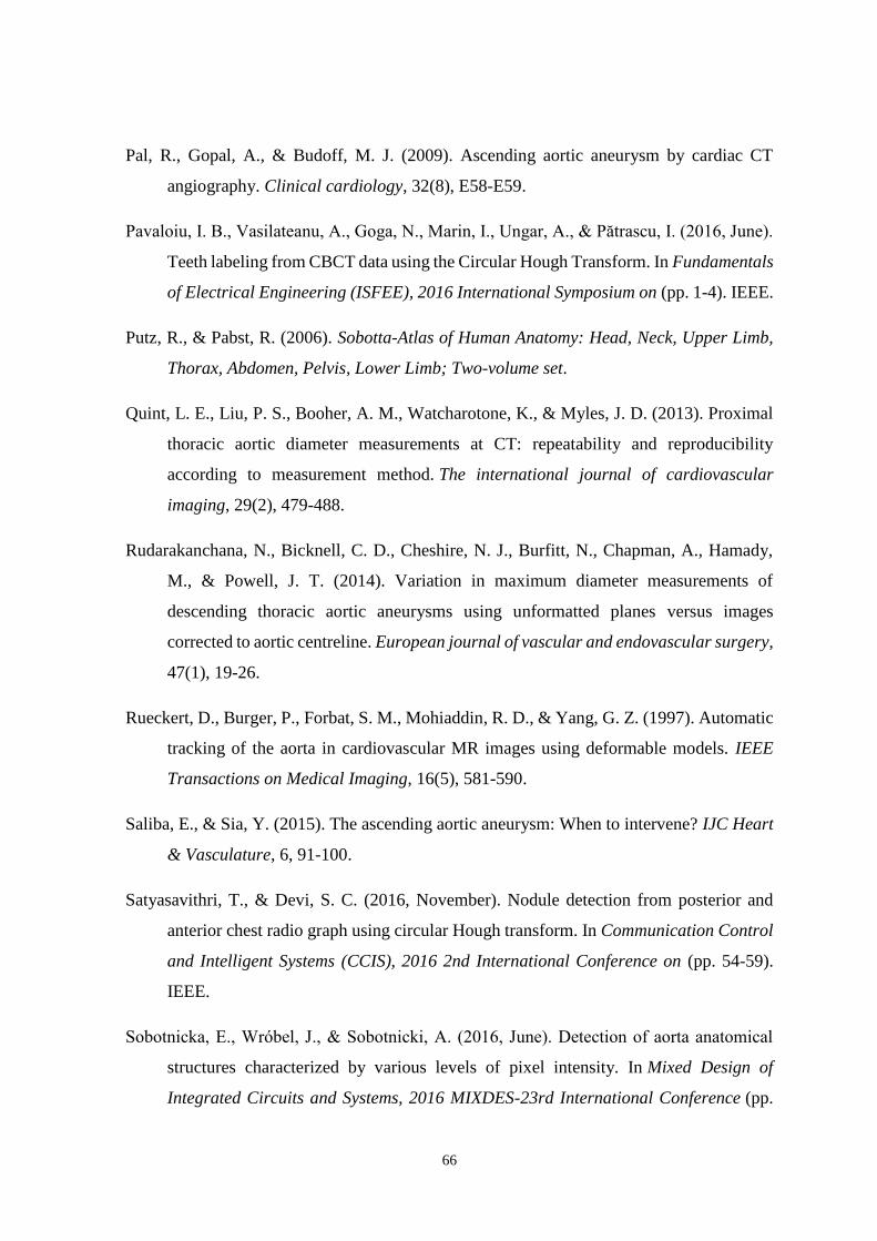
66
Pal, R., Gopal, A., & Budoff, M. J. (2009). Ascending aortic aneurysm by cardiac CT
angiography. Clinical cardiology, 32(8), E58-E59.
Pavaloiu, I. B., Vasilateanu, A., Goga, N., Marin, I., Ungar, A., & Pătrascu, I. (2016, June).
Teeth labeling from CBCT data using the Circular Hough Transform. In Fundamentals
of Electrical Engineering (ISFEE), 2016 International Symposium on (pp. 1-4). IEEE.
Putz, R., & Pabst, R. (2006). Sobotta-Atlas of Human Anatomy: Head, Neck, Upper Limb,
Thorax, Abdomen, Pelvis, Lower Limb; Two-volume set.
Quint, L. E., Liu, P. S., Booher, A. M., Watcharotone, K., & Myles, J. D. (2013). Proximal
thoracic aortic diameter measurements at CT: repeatability and reproducibility
according to measurement method. The international journal of cardiovascular
imaging, 29(2), 479-488.
Rudarakanchana, N., Bicknell, C. D., Cheshire, N. J., Burfitt, N., Chapman, A., Hamady,
M., & Powell, J. T. (2014). Variation in maximum diameter measurements of
descending thoracic aortic aneurysms using unformatted planes versus images
corrected to aortic centreline. European journal of vascular and endovascular surgery,
47(1), 19-26.
Rueckert, D., Burger, P., Forbat, S. M., Mohiaddin, R. D., & Yang, G. Z. (1997). Automatic
tracking of the aorta in cardiovascular MR images using deformable models. IEEE
Transactions on Medical Imaging, 16(5), 581-590.
Saliba, E., & Sia, Y. (2015). The ascending aortic aneurysm: When to intervene? IJC Heart
& Vasculature, 6, 91-100.
Satyasavithri, T., & Devi, S. C. (2016, November). Nodule detection from posterior and
anterior chest radio graph using circular Hough transform. In Communication Control
and Intelligent Systems (CCIS), 2016 2nd International Conference on (pp. 54-59).
IEEE.
Sobotnicka, E., Wróbel, J., & Sobotnicki, A. (2016, June). Detection of aorta anatomical
structures characterized by various levels of pixel intensity. In Mixed Design of
Integrated Circuits and Systems, 2016 MIXDES-23rd International Conference (pp.
67
498-503). Department of Microelectronics and Computer Science, Lodz University of
Technology.
Tokuyasu, T., Shuto, T., Yufu, K., Abe, H., Marui, A., Kanao, S., & Komeda, M. (2009,
December). Establishment of A Deformable Aorta Model Based on Patient's Chest CT
Data. In Innovative Computing, Information and Control (ICICIC), 2009 Fourth
International Conference on (pp. 1339-1342). IEEE.
Tortora, G. J., & Derrickson, B. H. (2009). Principles of anatomy and physiology. John
Wiley & Sons.
Umbaugh, S. E. (2005). Computer imaging: digital image analysis and processing. CRC
press.
Wilson, J. N., & Ritter, G. X. (2000). Handbook of computer vision algorithms in image
algebra. CRC press.
Wolak, A., Gransar, H., Thomson, L. E., Friedman, J. D., Hachamovitch, R., Gutstein, A.,
... & Hayes, S. W. (2008). Aortic size assessment by noncontrast cardiac computed
tomography: normal limits by age, gender, and body surface area. JACC:
Cardiovascular Imaging, 1(2), 200-209.
Zhu, X., & Rangayyan, R. M. (2008, August). Detection of the optic disc in images of the
retina using the Hough transform. In Engineering in Medicine and Biology Society,
2008. EMBS 2008. 30th Annual International Conference of the IEEE (pp. 3546-
3549). IEEE.