illiquidity measures and the pricing implication in ... measures and the pricing implication in...
TRANSCRIPT

1
Illiquidity Measures and the Pricing Implication
in Commercial Real Estate
Peng (Peter) Liu and Wenlan Qian*
*Liu is with the Department of Finance, Accounting and Real Estate, School of Hotel Administration,
Cornell University, Email: [email protected]. Qian (corresponding author) is with the Department of
Finance, National University of Singapore, Tel : (65) 65163015, [email protected].
2
I. Introduction
The relationship between illiquidity and asset prices has been examined extensively in the
stock and bond market, where the cross-sectional and time-series variation in price impact,1 is
empirically proven to be priced in the expected returns (e.g., Amihud and Mendelson, 1986;
Brennan, Chordia and Subramanyam, 1998; Amihud, 2002; Bekaet, Harvey and Lundblad, 2007;
Bao, Pan and Wang, 2010).2
Given the substantial evidence on the liquidity premium in other asset markets, it is a
plausible conjecture that liquidity plays a significant role in the real estate market, as real estate
transactions are very costly.3 On the other hand, the very long-term nature of investment in this
market makes the significance of the liquidity premium in real estate less obvious. Moreover, the
different market structure introduces new aspects of illiquidity that remain empirically under-
explored in the literature. In addition to other factors that drive illiquidity, 4 search efficiency is a
unique and significant aspect of trading frictions in the real estate market given the prolonged
negotiated transaction process that involves costly search and matching (e.g., Wheaton, 1990).
1 There is a large theoretical literature in microstructure that models illiquidity as the price concession required in
the presence of supply and demand imbalance as a result of asymmetric information, inventory risk and other effects
(Kyle, 1985; Glosten and Milgrom, 1985; Easley and O'Hara, 1987). 2In addition to the level of illiquidity, liquidity risk is shown to systematically influence asset prices in the stock
market (Pastor and Stambaugh, 2003; Acharya and Pedersen, 2005; Sadka, 2006) and in the bond market (Acharya,
Amihud, and Bharath, 2010; Li, Wang, Wu, and He, 2010; Lin, Wang, and Wu, 2010). 3 Transaction cost is estimated to be over three percent of the asset value (e.g., Haurin and Gill, 2002; Collett, Lizieri
and Ward, 2003). 4It is well accepted that leverage and the down payment constraint amplifies negative demand shocks (Stein, 1995;
Genesove and Mayer, 1997; Ortalo-Magne and Rady, 2006). Seller's behavioral limitation, such as loss aversion,
leads to a lower probability of sale and a longer time to sale (Genesove and Mayer, 2001; Engelhardt, 2003). Sellers
can also rationally delay sale timing due to the value of the option of waiting (Qian, 2012).

3
Despite its economic significance5, empirical examinations on the relationship between
illiquidity and real estate prices have been limited in scope. One major barrier to such endeavors
is data availability. First, real estate is infrequently traded and direct measures of liquidity (e.g.,
bid-ask spread) are unavailable. Second, the popular proxy for search frictions, time-on-market
(hereafter, TOM), is costly to gather for each individual transaction at the national level or for a
lengthy time period.
The objective of this paper is study illiquidity and its pricing implication in real estate.
Specifically, we focus on office buildings in the commercial real estate market. Buying and
selling commercial real estate, in contrast to residential real estate, is purely investment-driven
with the more sophisticated institutional investors being the major players. The office market is
the key market in commercial real estate market, with a market capitalization of 6.5 trillion US
dollars in the US at the end of 2010, which is slightly bigger than the U.S. treasury market and
over half of the entire commercial market. Furthermore, the unique institutional features of the
commercial real estate market make it ideal to identify search inefficiencies, a key aspect of
illiquidity in over-the-counter markets in general.
We propose real estate illiquidity measures that are readily obtainable from transaction
information. We take advantage of a salient feature of illiquidity in constructing our measures.
Specifically, illiquidity leads to deviation of the transaction price from the asset’s fundamental
value, regardless of the underlying causes. This observation helps avoid the need to model
directly the relevant determinants of illiquidity in real estate. Motivated by Amihud and
Mendelson (2002), we first propose a price impact measure to reflect illiquidity when there is an
5 Illiquidity has important implications for understanding the price determinants (e.g., Turnbull and Zahirovic-
herbert, 2010; Campbell, Giglio and Pathak, 2011), price index construction (Goetzmann and Peng, 2006) and
portfolio allocation (Lin and Vandell, 2007).

4
imbalance between supply and demand. It is defined by the (absolute) price change (in
percentage term) in market j from the time period t-1 to t divided by the dollar trading volume in
this market at time t. Conditional on the level of the trading activity, a larger price movement
implies a higher degree of illiquidity.
Moreover, we measure the market’s search inefficiency as the ratio of the price impact (𝜆)
measure of the subset of the less search-efficient properties in the same geographic market to that
of the submarket of more search-efficient properties. Large, institutional investors trade
commercial properties in a segmented market: typically they target larger, high quality, high-
value properties. These investors are well-informed about the properties on the market, and the
transactions are often taken place via auctions. In contrast, small, retail investors are more
restricted in the smaller, no-prime markets, and they have to engage in lengthy and costly search,
much as in the residential real estate, to complete the transaction. Therefore, within the same
geographical location, there are two types of office buildings that are subject to similar
macroeconomic fundamentals (such as local income and unemployment) but differ dramatically
in search costs. The difference in price impacts between small and big properties within a market
that shares the same fundamentals likely captures the level of search inefficiency in this
particular market at the time.
Using a national sample of office market transactions in the U.S. from 2000 to 2011, we
compute the two measures for each of 24 markets6 at the quarterly level. We first study the
applicability of the price impact and search friction measures by comparing them with
characteristics of these transactions that are correlated with supply-demand mismatch or search
frictions. Our proposed measures perform well. The price impact measure is negatively
6 The geographic market classification is defined by the data provider, CoStar COMP.

5
correlated with the trading volume, and is positively correlated with the proportion of distress
sales in the market at a given time. The search friction measure is positively associated with the
proportion of tax-deferred transactions and the proportion of properties sold with high vacancy
or to out-of-state buyers. It is negatively associated with the proportion of tenant purchases in
the market. Using the out-of-sample aggregate statistics on the commercial real estate market
(such as total trading volume), we confirm our in-sample findings.
We also study how these two liquidity measures are related with macroeconomic
variables. Price impact is significantly negatively correlated with local GMP and positively
related with local market unemployment rate and funding/lending availability. On the other hand,
the search friction measure is negatively associated with population density in the local market,
interest rate, and the cap rate in the local market. In summary, these results suggest that price
impact is positively associated with economic conditions, while search friction can be even more
relevant in “hot” markets.
Next, we investigate the pricing implication of illiquidity using the price impact and
search friction measures. Office buildings, both investment grade and non-investment grade, in
markets at times with high price impact tend to command a higher return over the subsequent
quarter. Search friction strongly predicts future returns in the non-investment grade submarket
with costly search. We further gauge the return-illiquidity relationship in different market
conditions. Illiquidity is likely to be particularly important during down markets (Brennan, Huh,
and Subrahmanyam, 2012), either due to higher liquidity risk (Acharya and Pedersen, 2005;
Acharyaet al., 2010) or due to capital constraints (Mitchell, Pedersen, and Pulvino, 2007;
Brunnermeier and Pedersen, 2009; Hameed, Kang, and Viswanathan, 2010). We create a down
market dummy for each market at quarter t if the quarter t return is negative. The illiquidity
6
premium is driven by the down period. For example, in the down market, a 10% increase in the
price impact measure is associated with 0.86% increase in the annualized expected return in the
cross section.
Lastly, we explore the variation in the liquidity premium among investment grade office
properties and non-investment grade buildings within the same geographic market. Search
friction is only relevant for future returns in the non-investment grade submarket. More
interestingly, there is a flight-to-quality (liquidity) during market downturns. During such times,
search friction and price impact strongly positively predict future returns in the non-investment
grade properties. However, a higher search friction in the entire market during the down market
predicts a negative return in the investment grade submarket over the next quarter. In addition,
price impact does not predict a higher return over the next quarter for the investment grade
properties at such times. These results suggest that investors flood to the submarket with better
liquidity (i.e., lower price impact and little search frictions on average) during market distress
and thus pay a price (liquidity) premium for the more liquid submarket.
The paper proceeds as follows. Section II introduces the two proposed illiquidity
measures used in the study. Section III describes the office market transaction data. Section IV
presents the empirical results, including evaluation of the price impact and search friction
measures as well as the pricing implications of illiquidity in the context of the US office market.
Section V concludes.
II. Measures of Illiquidity -- Price Impact (λ) and Search Friction
The first objective of this paper is to construct intuitive and easy-to-compute liquidity
proxies using readily available data in the real estate market. The Amihud measure (Amihud,
7
2002) aims to capture illiquidity using the magnitude of the price movement conditional on trade
size, and it performs well in capturing price impact (Goyenko, Holden and Trzcinka, 2009).
Given the low frequency of our data which limits the direct application of the Amihud measure,
we define our price impact proxy using price and volume data in a slightly different fashion.
𝜆 =| |
=
|
∑( )
∑( )
|
(1)
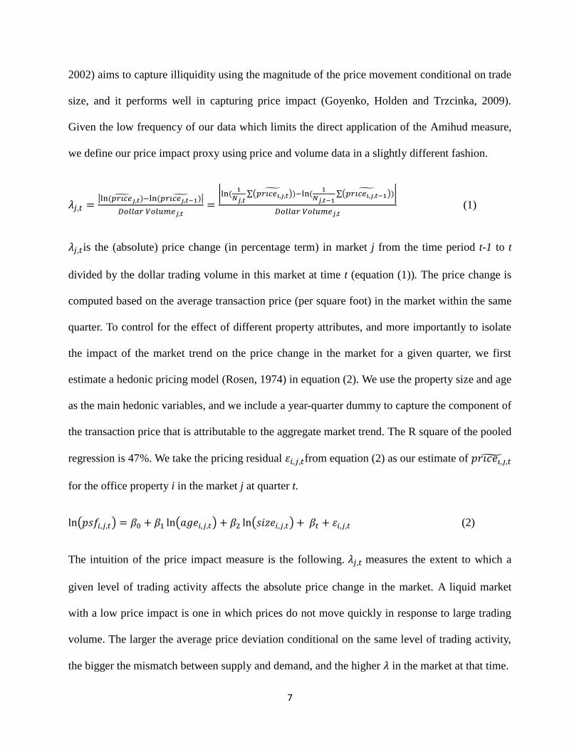
𝜆 is the (absolute) price change (in percentage term) in market j from the time period t-1 to t
divided by the dollar trading volume in this market at time t (equation (1)). The price change is
computed based on the average transaction price (per square foot) in the market within the same
quarter. To control for the effect of different property attributes, and more importantly to isolate
the impact of the market trend on the price change in the market for a given quarter, we first
estimate a hedonic pricing model (Rosen, 1974) in equation (2). We use the property size and age
as the main hedonic variables, and we include a year-quarter dummy to capture the component of
the transaction price that is attributable to the aggregate market trend. The R square of the pooled
regression is 47%. We take the pricing residual 𝜀 from equation (2) as our estimate of 𝑝𝑟𝑖𝑐𝑒
for the office property i in the market j at quarter t.
(𝑝 ) = ( 𝑒 ) ( 𝑒 ) 𝜀 (2)
The intuition of the price impact measure is the following. 𝜆 measures the extent to which a
given level of trading activity affects the absolute price change in the market. A liquid market
with a low price impact is one in which prices do not move quickly in response to large trading
volume. The larger the average price deviation conditional on the same level of trading activity,
the bigger the mismatch between supply and demand, and the higher 𝜆 in the market at that time.

8
It is important to note that the limited set of explanatory variables (and R square) in
equation (2) is not limitation of our pricing equation, as it is not meant to capture the hedonic
determinants of office properties prices. The purpose of the estimation is to remove persistent
time trends in prices given our low frequency observations, and is to control for the most salient
differences in building attributes (such as age and size) to allow a meaningful measure of
aggregate price and return. The residual estimate of 𝑝𝑟𝑖𝑐𝑒 should be interpreted as the de-
trended office price of building i in MSA j at quarter t, controlling for size and age. We allow our
estimate of 𝑝𝑟𝑖𝑐𝑒 to be a function of other property- or sale-specific attributes that may reflect
liquidity of the transaction. This facilitates our identification of the liquidity measures, which are
computed based on the estimated 𝑝𝑟𝑖𝑐𝑒 . It also allows the subsequent empirical tests of the
pricing of illiquidity based on changes in these prices.
The unique institutional features of the commercial real estate market make it ideal to
identify search inefficiencies. Large, institutional investors trade commercial properties in a
segmented market: typically they target larger, high quality, high-value properties. These
investors are well-informed about the properties on the market, and the transactions are often
taken place via auctions. In contrast, small, retail investors are more restricted in the smaller, no-
prime markets, and they have to engage in lengthy and costly search, much as in the residential
real estate, to complete the transaction. Therefore, within the same geographical location, there
are two types of office buildings that are subject to similar macroeconomic fundamentals (such
as local income and unemployment) but differ dramatically in search costs.
Given such, search friction is defined to be the ratio of the price impact (𝜆) measure of
the subset of the less search-efficient office properties in a particular geographic market and that
of the submarket with the more search-efficient properties (Eqn. (3)). The idea is that,

9
conditional on the average level of supply and demand mismatch in a given market, the
incremental price impact of the relatively search inefficient submarket compared to the search
efficient submarket measures the pricing outcome of search frictions. Based on the industry
convention, we define the class A and B office properties as the search-efficient properties, due
to high visibility and information transparency and since institutional investors are the major
players in this sub-market and the transaction process involves little search. Class C office
properties tend to be smaller, less expensive properties traded by retail investors with significant
search frictions. As a robustness, we also identify search- (in)efficient submarkets based on size
(either dollar value or the physical size). Small properties arguably have higher search frictions
than bigger properties due to lower visibility and match quality. The results are qualitatively the
same.
s𝑒 𝑟𝑐ℎ 𝑐𝑜 𝑡
=
≡
(3)
The main advantage of the two proposed measures is their simplicity and availability.
Price and volume information are always accessible in any standard real estate data and thus we
circumvent the need to access TOM data, which, as we indicated, are in general not readily
available. One can also model the price impact by estimating the latent supply and demand using
a structural approach (e.g., Fisher, et al., 2003, 2004). In this paper, we take advantage of a
salient feature of illiquidity in constructing our measures. Specifically, illiquidity leads to
deviation of the transaction price from the asset’s fundamental value, regardless of the
underlying causes. This observation helps avoid the need to model directly the relevant
determinants of illiquidity in real estate.

10
Our measures are alternative to traditional proxies in the real estate market such as
trading volume (or TOM). Specifically, they offer a more relevant proxy for understanding the
pricing implication of illiquidity. Firstly, as we stated, TOM is a(n endogenous) function of the
final transaction price. For example, a distressed sale with a heavy discount may have a low
TOM, which does not provide any information on the general search condition in the market at
that time. More generally, research shows the tradeoff between TOM and the selling price, which
is incorporated into a seller’s optimal listing decision (Haurin et al., 2010). Similarly, a large
trading volume that greatly affects the transaction price (e.g., a bulk of distress sales with heavy
price discounts) does not imply a liquid market. This suggests that one needs to incorporate price
impact in measuring liquidity. Secondly, realized TOM is a lagging indicator of the search
efficiency in the market, and thus is less helpful in understanding the expected returns. An
increase in the search friction is revealed in the TOM measure only after the properties are sold,
which could be long after the original shock. Lastly, we introduce both price impact and search
friction measures to distinguish the different aspects of illiquidity.
III. Data Description
A. Office market transaction data
Our sample consists of 88,561 office property transactions over a 144-month period
(from Jan. 2000 to December 2011) drawn from across 24 largest real estate markets in the
United States that span 15 states: Arizona, California, Colorado, Florida, Georgia, Illinois,
Massachusetts, Michigan, New Jersey, New York, Nevada, Oregon, Pennsylvania, Texas,
Washington, plus the District of Columbia. The data used in this study come from CoStar
COMPS, a proprietary database provided by the CoStar group (NASDAQ: CSGP).
11
Headquartered in Washington D.C., CoStar maintains the largest and most comprehensive
database of commercial real estate information7. CoStar collects data on commercial real estate
transactions by contacting buyers, sellers, and brokers. Each transaction is then researched and
verified by CoStar professionals to ensure accuracy. We are unaware of any sample selection
issues materially affecting the dataset8.
We removed all transactions that are indicated as non-arm’s length and deleted outliers of
size and price per square foot for those in the bottom 1%. We exclude transactions that are
historic sites or built-to-suit, those associated with condominiums conversions or assemblages, or
sales that involved damage from natural disasters or building contamination.The original dataset
contains a rich set of property-level hedonics as well as transaction-level information. However,
coverage varies among these variables. For example, not surprisingly, listing information,
appraisal value as well as TOM information is available for only a small subset of all the
transactions. To ensure power and accuracy of our analysis, we restrict ourselves to variables
with either no or few missing values. The only exception is TOM, which we still include for the
purpose of comparing with our own liquidity proxies.
We also obtain macroeconomic variables from different sources. The annual real Gross
Domestic Product per capita by Metropolitan area (GMP) is obtained from Bureau of Economic
Analysis under U.S. Department of Commerce. Population density (DENSITY) at MSA level is
retrieved from U.S. Census Bureau. The unemployment rate (UNEMP), obtained from Bureau of
Labor Statistics under U.S. Department of Labor, is a quarterly percentage of unemployment rate
at the applicable MSA. The average 30-year fixed rate mortgage (MB30), aggregated by the
7CoStar is the #1 commercial real estate company in the U.S. and U.K. Its proprietary database covers more than
two million properties and more than 37 billion square feet of inventory in all commercial property types and classes. 8Studies that use CoStar COMPS data include Benmelech, Garmaise, and Moskowitz (2005), Garmaise and
Moskowitz (2004).

12
Mortgage Bankers Association of America is used to measure the nation-wide real estate
financing cost9. TIGHTEN, the net percentage of banks tightening standards for commercial real
estate loans is from the quarterly senior loan officer opinion survey on bank lending practices.
The average capitalization rate (CapRate) is the ratio of property rental income net of operating
expenses divided by the transaction price, from the office sales reported by Real Capital
Analytics. INVENTORY is the total square footage of completed properties that are competitively
rented10
. OverSupply, calculated as amount of new space added to market inventory
(construction completions) during the time period divided by net change in occupied space
(absorption) during the same time period.
B. Descriptive statistics
Panel A of Table 1 presents summary statistics on the properties in our sample and some
key variables used in the analysis. Unit sale prices of office buildings range from $10.39 per
square feet to $5,416.67 per square feet, while the average sale price per square feet is $174.18.
Among 88,561 transactions that meet our data requirement, 35,243 sales contain information of
the time-on-market (TOM), which is the numbers of days between the sale date of an office
building and the date it is listed on the market.11
The selection bias is a major issue for TOM, so
we only use it as an indicative measure to compare with our liquidity proxies. Using the
available information, the average marketing time for an office building is 263.53 days. The
Building Age variable is computed as the difference between the property’s built year and year it
9 We use the MB30, a key rate used in deciding mortgage rates for home buyers as the benchmark for the real
estate market condition. Commercial mortgages are normally risker and of shorter term. However we don’t access
to the information of commercial mortgages rate.
10 Owner-occupied, medical office buildings and buildings under construction are excluded from the inventory.
11
We winsorize TOM at the top 1% tail.

13
is sold. The average building age is 34.79 years with standard deviation of 30.70 years.12
The
Building Size, measured as the total square footage of gross building area, varies significantly in
the sample with a mean of 27,443 square feet13
. The largest office building is about 3,781,045
square feet, while the smallest office space sold is only about eight hundred square feet. Class A
is a dummy variable with a value of 1 if the property is a class A office building and 0 otherwise.
Class A buildings are investment-grade properties that command the highest rents and sales
prices in a particular market.
[Insert Table 1 about here]
We further create several dummy variables indicating atypical sale conditions: Auction is
a dummy variable equal to 1 if the property is sold via auction and 0 otherwise; Distressed Sale
is a dummy variable equal to 1 if the property is sold as a distressed property and 0 otherwise,
1031 Exchange is a dummy variable equal to 1 if the property is sold as tax-deferred (1031
exchange) transaction and 0 otherwise, High Vacancy is a dummy variable equal to 1 if the
property’s vacancy rate is greater than 18% (sample median) or if the seller indicated that the
property is of a high vacancy condition, Tenant Purchase is a dummy variable equal to 1 if the
property is purchased by a current tenant and 0 otherwise, Out of State Buyer is a dummy
variable equal to 1 if the property is sold to an out-of -state (sometimes out-of-country) buyer.
The above atypical sale conditions are not mutually exclusive.
12
We treat the building age as zero, if the office building is sold in the same year or before the year it is built. 13
Because size is one of the most important building characteristics in commercial real estate valuation, we try to
verify and retrieve the size information as much as possible. If size variable in CoStar dataset is missing or
erroneous, we use the ratio of sale price over price per square feet. If price per square feet is missing or erroneous,
we compute the size using the product of number of floors and typical floor size. If none of the above information
available, we approximate the building size using land area size.
14
Panel B of Table 1 shows the number and percentage of transactions by market to
illustrate the geographical coverage of the data. Ranked by the total number of sales from 2000
to 2011, the sample includes 88,5361 office building sales in 24 largest real estate markets: New
York Metro14
, Los Angeles, Chicago, Washington D.C., South Florida, Phoenix, Atlanta, Denver,
Philadelphia, Boston, Seattle/Puget Sound, Tampa/St Petersburg, Orlando, Orange (California),
San Diego, Sacramento, Portland, East Bay/Oakland, Dallas/Ft Worth, Detroit, Inland Empire
(California), Las Vegas, South Bay/San Jose, and San Francisco. The top three markets: New
York Metro (7,766 transactions), Los Angeles (6,046 transactions), and South Florida (5,122
transactions) account for a quarter of the sales in the sample, while the smallest market in the
sample is San Francisco with 1,101 transactions. To reduce the influence of small sample bias
and ensure robustness of our results, we remove market-quarters that have fewer than 10
transactions from the main analysis.
IV. Empirical Findings
A. Empirical Estimates of λ and Search Friction
We estimate the hedonic pricing model in (2) in the pooled sample to obtain an estimate
of 𝑝𝑟𝑖𝑐𝑒 and the quarterly price 𝑃 for market j at quarter t (by averaging 𝑝𝑟𝑖𝑐𝑒 across all
transactions for market j at quarter t). Next, for each of the 24 office markets, we compute the
price impact (λ) and search friction measures according to (1) and (3) for each quarter from
2001:Q1 to 2011:Q4.15
Outliers of λ and search friction, defined to be the upper and lower 1%
14
The New York Metro market includes New York City, Northern New Jersey and Long Island. 15
In the main analysis, we restrict our sample to post-2000 due to a more comprehensive coverage of markets of
Costar after 2000.

15
tails, are winsorized. The values of both variables are roughly between 0.1 and 3 for all the
markets in our sample period.
Before we study the pricing implication of illiquidity, we first investigate the time-series
as well as cross-sectional properties of those measures. Table 2 provides annual time series of
quarterly average statistics of common proxies of liquidity and price per square foot in the
sample. The average price per square foot of transacted office properties in 24 markets, measured
as dollar per square foot, has increased steadily since 1995. It peaks in 2007 and decreases
afterwards. Both λ and search friction move over time but with a different pattern. In aggregate,
price impact is high at the beginning of the sample period, reaches the bottom in 2007, and
increases afterwards reaching the highest level after the 2008 crisis. This co-moves (negatively)
with the aggregate price trend. The search friction is also high in the early sample period which
decreases afterwards, but it also rises during the hot market period (2005-2007). At the beginning
of the crisis (2008), search friction does not immediately increase but it is significantly higher in
the period of 2009-2011.
[Insert Table 2 about here]
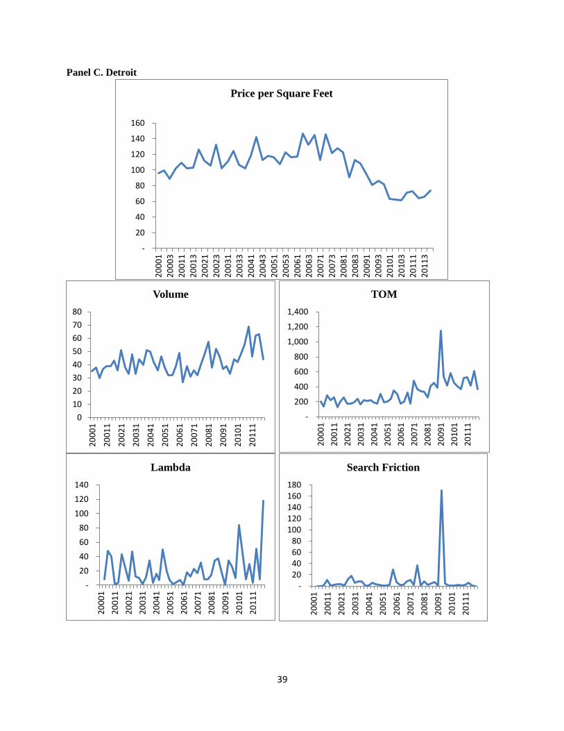
We further look into the cross-sectional variation in the time series pattern in Table 2.
Figure 1 plots price and liquidity dynamics over time in Los Angeles, New York Metro, Dallas
and Detroit markets. While there is commonality in the liquidity trends over time, both λ and
search friction exhibit cross-sectional variation across different markets. For example, there is a
much smaller increase in price impact in the New York metro market during the 2008 crisis,
compared with the Los Angeles market. On the other hand, New York experienced a serious
demand shock and high search frictions in the beginning of the sample period, resulting in a very
16
high value of λ, search friction and abnormally low trading volume. For the less metropolitan
markets such as Detroit and Dallas, the price impact and search friction series are much more
volatile, and they in general have a higher search friction measure than either Los Angeles or
New York Metro market.
[Insert Figure 1 about here]
B. Are the proposed liquidity proxies measuring liquidity in the real estate market?
We answer the question by examining the cross-sectional and time-series correlation
between our liquidity proxies and the variables that are shown to be related to the various
liquidity aspects.
Existing literature suggests several variables that are correlated with search frictions and
demand shocks. Campbell et al. (2010) suggest that distressed sales incur large price discounts,
reflecting the impact of illiquidity via supply-demand imbalance and search inefficiency in the
housing market. Turnbull and Sirmans (1993) find that out-of-state buyers pay a premium largely
due to high search frictions. Ling and Petrova (2010) suggest three sale conditions that imply
high search frictions in the commercial real estate market: tax-deferred (1031 exchange)
transaction, distressed sale and purchase by out-of-state buyers find consistent evidence.
Turnbull et al. (2010) show the vacancy effects on search friction and sale prices.
[Insert Table 3 about here]
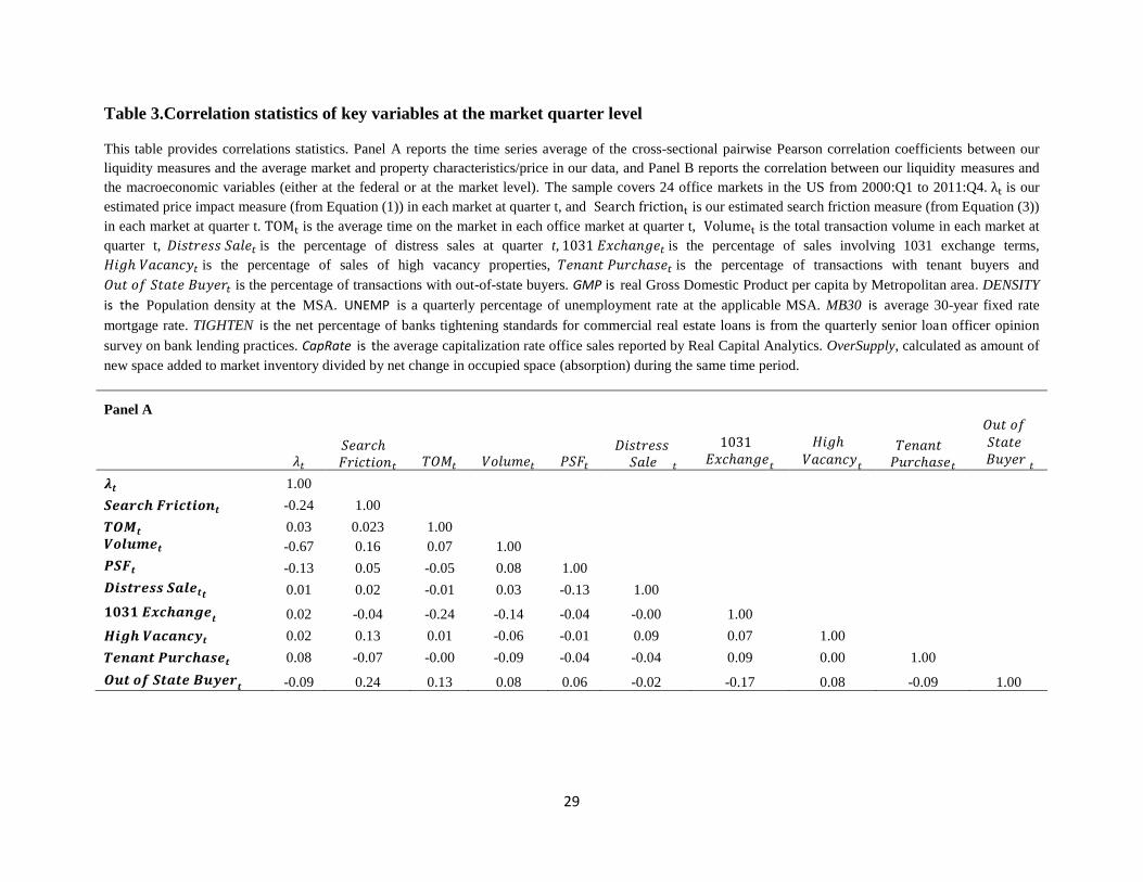
Table 3 Panel A reports time series average of cross-sectional pairwise Pearson
correlation coefficients among liquidity proxies and the market-specific and trade condition
variables obtained in our data at the quarterly level. The simple univariate exercise suggests that
our price impact and search friction measures are overall consistent with known proxies
17
suggested by the literature. λ is positively correlated the proportion of distress sales, tax-deferred
transactions, high vacancy buildings and tenant purchases in the market and negatively
correlated with the proportion of out-of-state buyers in the market as well as volume and average
transaction price. The search friction measure is positively related to TOM, high vacancy
properties and purchases by out-of-state buyers. It is negatively correlated with the proportion of
tenant purchases. In addition, λ and search friction is negatively correlated, suggesting that they
capture independent illiquidity aspects in the office market. In particular, the result that search
friction is positively correlated with transaction price and volume suggests that search friction is
significantly manifested in the “hot” market conditions, whereas price impact is more related to
bad market conditions.
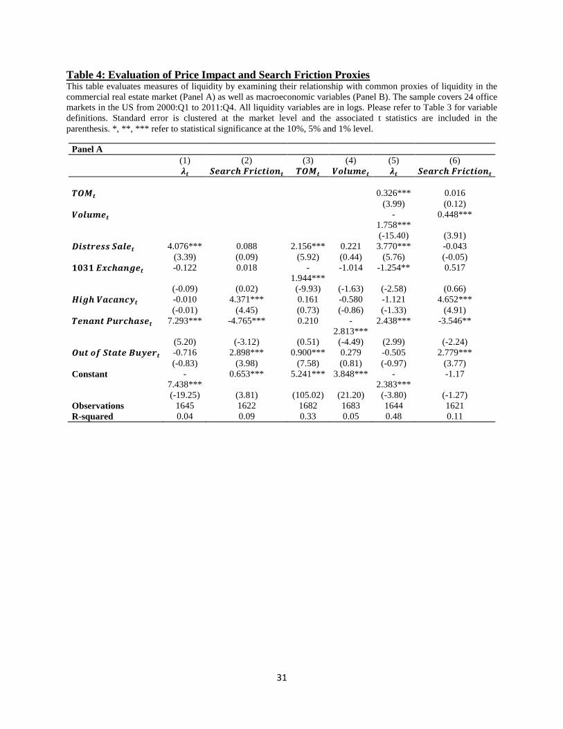
Table 4 examines the performance of various liquidity proxies in a multivariate
regression framework in the pooled sample. The multivariate results in general confirm the
findings in Table 3. λ is significantly positively correlated with the proportion of distress sales
and tenant purchases, and is negatively related with the proportion of tax-deferred exchange
transactions (Panel A). The search friction measure is significantly positively correlated with
high vacancy sales, out-of-state-buyer purchases, while it is negatively correlated with the
proportion of tenant purchases. Search friction is also positively correlated with the proportion of
tax-deferred exchange transactions, but it is not statistically significant.
[Insert Table 4 about here]
We run similar regressions using transaction volume and TOM as dependent variables
(columns 3-4 of Panel A, Table 4). Transaction volume is in general not related to known proxies
for illiquidity in the regression. There is a positive relationship between time on the market

18
(TOM) with the proportion of distress sales and out-of-state sales. However, TOM is also
significantly negatively correlated with the proportion of tax-deferred exchange transactions,
which is inconsistent with the prior literature that suggests that tax-deferred exchange
transactions typically incur higher search costs.
We also control for volume and TOM in evaluating the independent effects of our
liquidity proxies (column 5-6 of Panel A, Table 4). Our price impact (search friction) measure is
negatively (positively) correlated with transaction volume (TOM). In addition, previous results
still hold and remain strong. Taken together, these findings suggest that our proposed price
impact and search friction are reasonable liquidity proxies. Furthermore, they capture beyond
what is contained in the transaction volume and TOM. For example, a greater proportion of
distress sales in a market at a given quarter is associated with a higher price impact, an insight
shared by Campbell, et al. (2009). However, volume has an insignificantly positive relationship
with the proportion of distress sales.
C Price Impact, Search Friction and Macroeconomic Conditions
Next, we investigate how our price impact and search friction variables are correlated with the
macroeconomic variables. We also use the aggregate statistics on the commercial real estate
market conditions as an out-of-sample test of our findings in Panel A of Table 3 and 4. Panel B
of Table 3 reports the simple correlation statistics between our liquidity measures and
macroeconomic variables. Price impact, 𝜆, is negatively correlated with local GMP, suggesting
that liquidity is low resulting in a high price impact when the local market has low productivity.
Similarly, a high price impact is associated with a high unemployment rate, high cap rate, a
tighter lending standard, or a lower interest rate. Our price impact is also positively correlated

19
with high vacancy and negatively correlated with total trading volume in that local area, which
confirm our in-sample finding in Panel A of Table 3.
Search friction is strongly negatively related to population density, consistent with
traditional search theory. It is positively correlated with GMP, total trading volume and
negatively correlated with unemployment and cap rate, suggesting that search frictions can be
relevant in good economic conditions. For example, in “hot” markets, there are more buyers in
the market and the seller’s option value of waiting for a more attractive offer is higher, resulting
in a less efficient searching and matching outcome (Novy-Marx, 2009).
In Panel B of Table 4, we carry out multivariate regressions. In columns (1)-(2), we
regress our liquidity measures on macroeconomic variables (at the national level). In columns
(3)-(4), we regress liquidity measures on the commercial real estate market-specific variables (at
the market level). Results are qualitatively the same as the simple correlation statistics in Panel B
of Table 3. Price impact is strongly negatively correlated with local GMP, total trading volume,
and is positively correlated with unemployment rate, funding/lending availability and high
vacancy. Similarly, search friction is strongly negatively correlated with population density,
interest rate and cap rate. Coefficients on other variables are statistically insignificant.
D The Relationship Between Expected Return and Illiquidity in the Office Market
Next we study whether the illiquidity level is priced in the expected returns in the office market
in the U.S. We perform Fama-Macbeth regressions and the dependent variable is the one-
quarter-ahead change in price as measured by the average transaction price (after de-trending and
controlling for age and size, i.e., from Equation (2)). All liquidity variables are in logs. We
also include the macro variables as control variables in columns (4)-(6) of Table 5.

20
[Insert Table 5 about here]
High λ this quarter leads to a positive return over the next quarter, with or without
controlling for the macroeconomic variables (Table 5). The effects are statistically significant at
the 5% level. To interpret, a 10% increase in λ is associated with an increase in 10 basis points
over the next quarter. In contrast, in the full sample of the office market, search friction does not
seem to be relevant for the average office building prices, as a high search friction this quarter is
not associated with the return in the subsequent quarter, with or without controlling for the
macroeconomic variables.
E Illiquidity Premium in the Normal versus Down Markets
The existing evidence in the literature points to a strong positive relationship between
price impact and future returns, and results in Table 5 lend further support to the illiquidity-
expected return relationship in the context of real estate. We next investigate whether the
liquidity premium is particularly relevant in some periods or market conditions rather than others.
A priori, illiquidity premium varies over time and is a function of the market conditions. In the
real estate market, it is a general phenomenon that liquidity tends to dry up in crashes or in
downturns (Stein, 1995; Krainer, 2001; Qian, 2012). Recent literature suggests that liquidity is
more valuable in such times and extra compensation is required (Mitchell et al., 2007;
Brunnermeier and Pedersen, 2009; Hameed et al., 2010; Brennan, et al., 2012).
We investigate the implication of illiquidity premium in different market conditions in
Table 6. We create a dummy, Down Market, that is equal to one if the quarterly return of a
market at quarter t is negative. By using zero return as the cut-off, our down market proxy is less
subject to a look-ahead bias, compared to other thresholds based on the in-sample return

21
distribution. We interact our liquidity proxies with the down market dummies and repeat the
analysis as in Table 5.
[Insert Table 6 about here]
Results in Table 6 present strong evidence consistent with our hypothesis. The premium
associated with the price impact measure is driven by the down market. In the down market, a 10%
increase in λ leads to a return increase of 26bps over the next quarter (statistically significant at
the 1% level), which translates into 0.84% excess returns per annum. On the other hand, search
friction proxy remains to have little predictive power on subsequent quarter returns in the full
sample of office properties, regardless of down market or not.
F Investment Grade versus Non-Investment Grade
As argued earlier, search friction is primarily relevant for the submarket where retail
investors are the major players. Therefore, ex ante, one should the search friction measure to be
priced in that submarket (instead of the full sample of office properties). In this subsection, we
study the cross-sectional difference in the illiquidity premium associated with both search
friction and price impact among different subsets of the office properties. We divide the market
into Class A/B and Class C office properties, and examine the illiquidity-expected return
relationship for the two sub-markets respectively. Class A and Class B buildings are more of
investment-grade properties with higher quality, higher price and a larger institutional investor
concentration. Class C buildings are typically smaller, cheaper and retail-investor-oriented. The
dependent variable is the one-quarter-ahead return based on the average transaction price per
square foot ( from Equation (2)) for the two submarkets within the same geographic market j
at time t respectively.

22
[Insert Table 7]
In all time periods, we continue to observe that price impact predicts the one-quarter-head
return, as in Table 5 and 6 (Panel A of Table 7). However, the predictive power is driven by the
positive relationship between price impact and future return in the investment grade properties.
On the other hand, in the non-investment grade submarket, the positive relationship between
price impact and future return is statistically insignificant. However, for that submarket, search
friction plays an important role in pricing the office buildings, consistent with the notion that
search friction is concentrated in the non-investment grade buildings. A 10% higher search
friction is associated with 8 bps higher return over the next quarter in the non-investment grade
submarket.
In Panel B of Table 7, we interact the liquidity measures with the down market dummy in
the submarket analysis. The search premium for the non-investment grade properties is
concentrated in the down market. In addition, price impact is priced in the non-investment grade
properties in distress market times (column (2) and (4)). More interestingly, for the investment
grade submarket in which liquidity is comparatively higher, the one-quarter-ahead return is more
negative when the overall office market in that area experiences a shock in search frictions. In
addition, during the down market, a price impact does not predict a higher return over the next
quarter for the investment grade properties. Taken together, this set of results are consistent with
the notion of flight-to-quality (-liquidity) in the 2008 crisis (e.g., Acharya et al., 2010) in the
office market. It suggests that, during market downturns, investors flood to the submarket with
better liquidity (i.e., lower price impact and little search frictions on average) and thus pay a
price (liquidity) premium for the more liquid submarket.
23
V. Concluding Remarks
We examine the pricing implication of illiquidity in a very illiquid market—real estate.
Specifically, transactions in this market occur over-the-counter with costly search and bilateral
bargaining. Direct measures of illiquidity are unavailable due to low transaction frequency and
data quality issues. We compute two indirect illiquidity measures from transaction price and
volume data. The first illiquidity proxy measures price impact, and the second illiquidity proxy
measures the search friction that is a significant source of illiquidity in this market.
Using a national sample of transactions in 24 major office markets in the U.S. from 2000
to 2011, we show that illiquidity is an important determinant of expected returns in commercial
real estate. The conventional illiquidity measure, price impact, is strongly priced in the market.
Search frictions, on the other hand, are also associated with future returns in the submarket with
costly search. The illiquidity premium is stronger in market downturns. Moreover, we find
evidence consistent with a flight-to-quality effect during the down markets. Specifically, at such
times, investors are willing to pay a higher price for more liquid properties in the investment-
trade submarket, while requiring a higher price discount in the less liquid, non-investment grade
submarket.
References
Acharya, V. and L. H. Pedersen, 2005. "Asset Pricing with Liquidity Risk."Journal of Financial
Economics 77, 375-410.
Acharya, V. Y. Amihud, and S. Bharath. 2010. “Liquidity Risk of Corporate Bond Returns.” Working
Paper
Amihud, Y., 2002. "Illiquidity and stock returns: Cross-section and time series effects."Journal of
Financial Markets 5(1), 31-56.

24
Amihud, Y. and H. Mendelson, 1986. "Asset pricing and the bid-ask spread."Journal of Financial
Economics 17, 223-249.
Bao, J., J. Pan, and J. Wang., 2010. “The Illiquidity of Corporate Bonds.” Journal of Finance,
forthcoming
Bekaet, G., Harvey, C., and Lundblad, C., 2007, "Liquidity and Expected Returns: Lessons from
Emerging Markets," Review of Financial Studies, 20(6), pp. 1783-1831
Benmelech, E., M.J. Garmaise and T. J. Moskowitz, 2005. "Do liquidation values affect financial
contracts? Evidence from commercial loan contracts and zoning regulation."Quarterly Journal
ofEconomics, 120 (3), 1121- 1154.
Brennan, M. J., Chordia, T., Subrahmanyam, A., 1998. "Alternative factor specifications, security
characteristics, and the cross-section of expected stock returns." Journal of Financial Economics 49, 345-
373.
Brennan, Michael., Sahn-Wook Huh and Avanidhar Subrahmanyam, 2012, “An Analysis of the Amihud
Illiquidity Premium.” Working Paper
Brunnermeier, Markus and Lasse Pedersen, 2009. "Market liquidity and funding liquidity." Review of
Financial Studies 22, 2201-2238.
Campbell, J., Giglio, S. and Pathak, P., 2011. "Forced Sales and House Prices", American Economic
Review 101:2108-2131.
Collett, D., C. Lizieri and C. Ward, 2003. "Timing and the holding periods of institutional real estate."
Real Estate Economics, 31 (2), 205- 222.
Duffice, Darrell, 1996. “Special repo rates.” Journal of Finance, 51, 493-526.
Duffie, Darrell, Nicolae Garleanu, and Lasse Heje Pedersen, 2002. “Securities lending, shorting, and
pricing,” Journal of Financial Economics, 66, 307-339.
Duffie, Darrell, Nicolae Garleanu, and Lasse Heje Pedersen, 2005. “Over-the-Counter Markets,”
Econometrica, 73, 1815-1847.
Duffie, Darrell, Nicolae Garleanu, and Lasse Heje Pedersen, 2007. “Valuation in Over-the-Counter
Markets,” The Review of Financial Studies, 20, 1865-1900.
Easley, David and O'Hara, Maureen, 1987. "Price, trade size, and information in securities
markets," Journal of Financial Economics, 19(1), pp. 69-90
Englehardt, G., 2003. "Nominal Loss Aversion, Housing Equity Constraints, andHousehold Mobility:
Evidence from the United States." Journal of Urban Economics, 53, 171-195.
Fisher, J., Gatzlaff, D., Geltner, D. And Haurin, D.,2003. "Controlling for the Impact of Variable
Liquidity in commercial Real Estate Price Indices."Real Estate Economics, 31(2) pp.269-303.
25
Fisher, J., Gatzlaff, D., Geltner, D. And Haurin, D. 2004. "An Analysis of the Determinants of
Transaction Frequency of Institutional commercial Real Estate Investment Property."Real Estate
Economics, 32(2) pp.239-264.
Garmaise, M.J., and Tobias J. Moskowitz."Confronting Information Asymmetries: Evidence from Real
Estate Markets." Review of Financial Studies, XVII (2004), 405–437.
Genesove, D., Mayer, C., 1997. "Equity and time to sale in the real estate markets." American Economic
Review 87, 255–269.
Genesove, D., Mayer, C., 2001. "Loss aversion and seller behavior: Evidence from the housing
market."The Quarterly Journal of Economics 116, 1233–1260.
Glosten, Lawrence R., and Paul Milgrom, 1985. “Bid, Ask and Transaction Prices in a Specialist Market
with Heterogeneously Informed Traders.” Journal of Financial Economics 14, 71–100.
Goetzmann, W., and Peng, L., 2006. "Estimating House Price Indexes in the Presence of Seller
Reservation Prices.” Review of Economics and Statistics, 2006, 88(1), 100-112
Goyenko, Ruslan Y., Craig W. Holden and Charles A. Trzcinka. 2009. "Do liquidity measures measure
liquidity?" Journal of Financial Economics 92: 153-181.
Hameed, Allaudeen, Wenjin Kang and S Viswanathan, 2010. "Stock Market Declines and
Liquidity” Journal of Finance 65(1) pp.257–293
Haurin, D. and H.L. Gill, 2002. “The impact of transaction costs and the expected length of stay on
homeownership”, Journal of Urban Economics, 51, 563- 584.
Haurin, Donald R., Jessica L. Haurin, Taylor Nadauld and Anthony Sanders. 2010."List prices, sale prices
and marketing time: An approach to U.S. housing markets." Real Estate Economics 38:659-685.
Krainer, J., 2001. "A theory of liquidity in residential real estate markets." Journal of Urban Economics
49, 32–53.
Kyle, Albert S.,1985. “Continuous Auctions and Insider Trading.” Econometrica 53, pp 1315–1335.
Li, Haitao, J. Wang, C. Wu, and Y. He, 2009. “Are Liquidity and Information Risks Priced in the
Treasury Bond Market?” Journal of Finance 64, pp. 467-503.
Lin, Hai, Junbo Wang and Chunchi Wu, 2011. “Liquidity risk and expected corporate bond returns.”
Journal of Financial Economics 99(3), pp. 628-650
Lin, Zhengguo and Kerry Vandell, 2007. "Illiquidity and pricing biases in the real estate market." Real
Estate Economics 35: 291-330.
Ling, D., and Petrova, M 2010. "Heterogeneous Investors, Negotiation Strength & Asset Prices in Private
Markets: Evidence from Commercial Real Estate." Working paper

26
Mitchell, Mark, Lasse Heje Pedersen, and Todd Pulvino, 2007, "Slow moving capital", American
Economic Review Papers and Proceedings 97, pp.215-220.
Novy-Marx, R., 2009. "Hot and cold markets." Real Estate Economics 37, pp.1–22.
Ortalo-Magne, F. and Rady, S., 2006. "Housing Market Dynamics: On the Contribution of Income
Shocks and Credit Constraints", Review of Economics Studies 73(2) pp. 459-485
Pástor, L., Stambaugh, R.F., 2003. "Liquidity risk and expected stock returns." Journal of Political
Economy 111, 642-685.
Qian, Wenlan, 2012. "Why do sellers hold out in the housing market? An option-based explanation." Real
Estate Economics, forthcoming.
Rosen, S., 1974. “Hedonic Prices and Implicit Markets: Product Diffentiation in Pure Competition.”
Journal of Political Economy 82:1, 34-55.
Sadka, Ronnie, 2006. “Momentum and post-earnings-announcement-drift anomalies: the role of liquidity
risk". Journal of Financial Economics 80, 309-349.
Stein, J., 1995. "Prices and trading volume in the housing market: A model with down payment effects."
The Quarterly Journal of Economics 110, 379–406.
Turnbull, G.K. and C.F. Sirmans, 1993. “Information, Search, and House Prices.” Regional Science and
Urban Economics, 23, 545-557.
Turnbull, G. K. and Velma Zahirovic-herbert. 2011. "Why do vacant houses sell for less: holding costs,
bargaining power or stigma?" Real Estate Economics 39: 19-43.
Wheaton, W., 1990. "Vacancy, search and prices in a housing market matching model." Journal of
Political Economy 98, 1270–1292.

27
Table 1. Summary Statistics
Panel A of this table provides summary statistics of the hedonic and sale-condition dummy variables used in the
study, and Panel B provides the geographic distribution of data (market is defined by the data provider CoStar
COMPS). The sample covers 24 office markets in the U.S. from 2000:Q1 to 2011:Q4. Price per s.f.is sale price per
square foot, TOM is time on market in days, Building Age is the number of years between the building’s sale date
and its built year, Building Size is total square foot of building space, Auction is a dummy variable with value of 1 if
the property is sold via auction and 0 otherwise; Distressed Sale is a dummy variable with value of 1 if the property
is sold as a distressed property and 0 otherwise, 1031 Exchange is a dummy variable with value of 1 if the property
is sold as tax-deferred (1031 exchange) transaction and 0 otherwise, High Vacancy is a dummy variable with value
of 1 if the property’s vacancy rate is greater than 18% (sample median) or the seller indicated that the property is of
a high vacancy condition , Tenant Purchase is a dummy variable with value of 1 if the property is purchased by a
current tenant and 0 otherwise, Out of State Buyer is a dummy variable with value of 1 if the property is sold to an
out-of -state (sometimes out-of-country) buyer, Class A is a dummy variable with value of 1 if the property is a class
A office building and 0 otherwise. Small buildings are defined to be those below the market-specific median of the
size distribution.
Panel A
Variables N Mean StdDev Min Max
Price per s.f. ($) 84,069 174.178 140.34 10.39 5,4016.67
TOM (day) 35,243 263.53 301.42 1 1,111
Building Age (year) 79,510 34.79 30.70 0 291
Building Size (s.f.) 88,561 27,443 84,7332 842 3,781,045
Class A (%) 88,561 6.27 N.A. 0 1
Distressed Sale (%) 88,561 2.84 N.A. 0 1
1031 Exchange (%) 88,561 6.47 N.A. 0 1
High Vacancy (%) 88,561 8.60 N.A. 0 1
Tenant Purchase (%) 88,561 2.20 N.A. 0 1
Out of State Buyer (%) 88,561 14.76 N.A. 0 1
Panel B
Location N % Location N %
New York Metro 7,766 8.77 Seattle/Puget Sound 2,348 2.65
Los Angeles 6,046 6.83 Orange (CA) 2,209 2.49
South Florida 5,122 5.78 San Diego 2,203 2.49
Phoenix 4,645 5.24 Dallas 2,049 2.31
Chicago 4,642 5.24 Detroit 1,980 2.24
Philadelphia 4,433 5.01 Sacramento 1,933 2.18
Atlanta 4,200 4.74 Inland Empire (CA) 1,868 2.11
Washington D.C. 4,000 4.52 Las Vegas 1,801 2.03
Denver 3,688 4.16 East Bay/Oakland 1,733 1.96
Tampa/St Petersburg 3,189 3.60 Portland 1,703 1.92
Boston 2,922 3.30 South Bay/San Jose 1,320 1.49
Orlando 2,448 2.76 San Francisco 1,101 1.24
Total 88,561 100

28
Table 2. Time Series Pattern of Price and Illiquidity proxies
This table provides annual time series of quarterly average statistics of common proxies of liquidity and price per
square foot in the commercial real estate market. The sample covers 24 office markets in the US from 2000:Q1 to
2011:Q4. is our estimated price impact measure in each market at quarter t(Equation(1)), and is
our estimated search friction measure in each market at quarter t(Equation (3)). Our two liquidity measures are
winsorized at the 1% and 99% level. is the average time on the market in each office market at quarter t,
is the total transaction volume in each market at quarter t.
Year λ (Basis Points) Search Friction Volume TOM PSF
2000 31.674 34.16 44.94 177.56 120.70
2001 35.596 21.54 42.04 173.85 144.10
2002 29.958 15.21 47.58 110.11 136.61
2003 26.777 11.45 50.89 158.94 144.12
2004 21.325 27.21 60.11 128.05 149.91
2005 15.652 42.47 53.55 177.39 178.34
2006 13.389 26.94 56.08 199.43 179.23
2007 10.788 34.70 66.90 249.38 206.36
2008 20.251 19.43 56.35 297.81 205.03
2009 46.104 21.81 40.01 311.14 162.91
2010 44.099 42.38 49.41 324.36 155.49
2011 51.519 44.63 61.11 461.41 134.84
29
Table 3.Correlation statistics of key variables at the market quarter level
This table provides correlations statistics. Panel A reports the time series average of the cross-sectional pairwise Pearson correlation coefficients between our
liquidity measures and the average market and property characteristics/price in our data, and Panel B reports the correlation between our liquidity measures and
the macroeconomic variables (either at the federal or at the market level). The sample covers 24 office markets in the US from 2000:Q1 to 2011:Q4. is our
estimated price impact measure (from Equation (1)) in each market at quarter t, and is our estimated search friction measure (from Equation (3))
in each market at quarter t. is the average time on the market in each office market at quarter t, is the total transaction volume in each market at
quarter t, 𝑡𝑟𝑒 𝑒 is the percentage of distress sales at quarter t, 𝑐ℎ 𝑒 is the percentage of sales involving 1031 exchange terms,
ℎ 𝑐 𝑐 is the percentage of sales of high vacancy properties, 𝑒 𝑡 𝑃 𝑟𝑐ℎ 𝑒 is the percentage of transactions with tenant buyers and
𝑡 𝑜 𝑡 𝑡𝑒 𝑒𝑟 is the percentage of transactions with out-of-state buyers. GMP is real Gross Domestic Product per capita by Metropolitan area. DENSITY
is the Population density at the MSA. UNEMP is a quarterly percentage of unemployment rate at the applicable MSA. MB30 is average 30-year fixed rate
mortgage rate. TIGHTEN is the net percentage of banks tightening standards for commercial real estate loans is from the quarterly senior loan officer opinion
survey on bank lending practices. CapRate is the average capitalization rate office sales reported by Real Capital Analytics. OverSupply, calculated as amount of
new space added to market inventory divided by net change in occupied space (absorption) during the same time period.
Panel A
𝜆
𝑒 𝑟𝑐ℎ 𝑟 𝑐𝑡 𝑜
𝑜 𝑒 𝑃
𝑡𝑟𝑒 𝑒
𝑐ℎ 𝑒
ℎ
𝑐 𝑐
𝑒 𝑡 𝑃 𝑟𝑐ℎ 𝑒
𝑡 𝑜 𝑡 𝑡𝑒 𝑒𝑟
1.00
-0.24 1.00
0.03 0.023 1.00
-0.67 0.16 0.07 1.00
-0.13 0.05 -0.05 0.08 1.00
0.01 0.02 -0.01 0.03 -0.13 1.00
0.02 -0.04 -0.24 -0.14 -0.04 -0.00 1.00
0.02 0.13 0.01 -0.06 -0.01 0.09 0.07 1.00
0.08 -0.07 -0.00 -0.09 -0.04 -0.04 0.09 0.00 1.00
-0.09 0.24 0.13 0.08 0.06 -0.02 -0.17 0.08 -0.09 1.00

30
Panel B
λ Search Friction GMP DENSITY UNEMP VOLUME CapRate TIGHTEN OverSupply MB30
λ 1
Search Friction -0.08 1
GMP -0.23 0.06 1
DENSITY -0.11 -0.11 0.06 1
UNEMP 0.28 0.00 -0.18 0.14 1
VOLUME -0.40 0.12 0.46 0.10 -0.35 1
CapRate 0.17 -0.08 -0.25 0.02 0.07 -0.40 1
TIGHTEN 0.02 -0.07 -0.01 0.00 0.21 -0.19 -0.01 1
OverSupply 0.00 0.04 -0.11 -0.08 0.00 0.04 -0.06 0.00 1
MB30 -0.11 -0.03 -0.01 -0.06 -0.65 0.16 0.13 0.15 0.00 1
31
Table 4: Evaluation of Price Impact and Search Friction Proxies This table evaluates measures of liquidity by examining their relationship with common proxies of liquidity in the
commercial real estate market (Panel A) as well as macroeconomic variables (Panel B). The sample covers 24 office
markets in the US from 2000:Q1 to 2011:Q4. All liquidity variables are in logs. Please refer to Table 3 for variable
definitions. Standard error is clustered at the market level and the associated t statistics are included in the
parenthesis. *, **, *** refer to statistical significance at the 10%, 5% and 1% level.
Panel A
(1) (2) (3) (4) (5) (6)
0.326*** 0.016
(3.99) (0.12)
-
1.758***
0.448***
(-15.40) (3.91)
4.076*** 0.088 2.156*** 0.221 3.770*** -0.043
(3.39) (0.09) (5.92) (0.44) (5.76) (-0.05)
-0.122 0.018 -
1.944***
-1.014 -1.254** 0.517
(-0.09) (0.02) (-9.93) (-1.63) (-2.58) (0.66)
-0.010 4.371*** 0.161 -0.580 -1.121 4.652***
(-0.01) (4.45) (0.73) (-0.86) (-1.33) (4.91)
7.293*** -4.765*** 0.210 -
2.813***
2.438*** -3.546**
(5.20) (-3.12) (0.51) (-4.49) (2.99) (-2.24)
-0.716 2.898*** 0.900*** 0.279 -0.505 2.779***
(-0.83) (3.98) (7.58) (0.81) (-0.97) (3.77)
Constant -
7.438***
0.653*** 5.241*** 3.848*** -
2.383***
-1.17
(-19.25) (3.81) (105.02) (21.20) (-3.80) (-1.27)
Observations 1645 1622 1682 1683 1644 1621
R-squared 0.04 0.09 0.33 0.05 0.48 0.11

32
Panel B
(1) (2) (4) (5)
-2.478* 0.605
(-1.99) (0.71)
-0.202 -0.470***
(-0.56) (-2.94)
0.172** -0.091
(2.61) (-1.60)
-0.035 -0.334**
(-0.24) (-2.25)
0.004* -0.000
(1.72) (-0.12)
-0.585*** 0.365***
(-5.30) (3.76)
-1.509 -15.319**
(-0.26) (-2.65)
-0.001* 0.001**
(-1.88) (3.73)
0.093*** 0.050
(4.76) (1.37)
Constant 19.638 0.442 8.724*** -4.740**
(1.40) (0.04) (3.46) (-1.03)
Observations 1177 1172 990 989
R-squared 0.14 0.04 0.36 0.07

33
Table 5.The Effect of Liquidity Measures on Quarterly Returns in the Office Market
This table studies whether the liquidity level is priced in the quarterly returns in the office market in the US. We
perform Fama-Macbeth regressions in the sample of 24 office markets in the US from 2000:Q1 to 2011:Q4. All
liquidity variables are in logs. The return variable is the quarterly change in the average trend-adjusted and
characteristic-adjusted price (i.e., estimated from Equation (2) in each office market at quarter t). is our
estimated price impact measure (from Equation (1)) in each market at quarter t-1, and is our
estimated search friction measure (from Equation (3)) in each market at quarter t-1. Please refer to Table 3 for
variable definitions of other explanatory variables. The associated t statistics are included in the parenthesis. *, **,
*** refer to statistical significance at the 10%, 5% and 1% level.
(1) (2) (3) (4) (5) (6)
VARIABLES
0.010*** 0.009*** 0.009** 0.009*
(3.08) (2.91) (2.22) (2.04)
-0.000 0.001 -0.003 -0.002
(-0.04) (0.24) (-1.23) (-1.06)
-0.210 -0.375 -0.163
(-0.80) (-1.46) (-0.66)
-0.520 -0.253 -0.552
(-0.78) (-0.38) (-0.77)
-0.001 -0.002 -0.001
(-0.14) (-0.27) (-0.16)
0.007 0.005 0.006
(0.65) (0.49) (0.58)
Constant 0.057*** 0.002 0.056*** 5.999* 5.914* 5.735*
(2.85) (0.67) (2.82) (1.84) (1.96) (1.74)
Observations 1607 1585 1585 1177 1172 1172

34
Table 6: Liquidity Premium in the Normal versus Down Markets
This table studies the liquidity effect in explaining returns in normal versus down market conditions using Fama-
Macbeth regressions. The sample covers 24 office markets in the US from 2000:Q1 to 2011:Q4. All liquidity
variables are in logs. 𝑜 𝑟 𝑒𝑡 is a dummy that takes 1 if the quarterly return (i.e., the quarterly change in
detrended and characteristics-adjusted prices) for a market at quarter t-1 is negative. Please refer to Table 3 for
definitions of the rest of the variables. The associated t statistics are included in the parenthesis. *, **, *** refer to
statistical significance at the 10%, 5% and 1% level.
(1) (2) (3)
0.448*** 0.121*** 0.451***
(9.92) (12.03) (9.36)
-0.020*** -0.019**
(2.97) (2.53)
0.004 0.002
(1.01) (0.54)
0.046*** 0.047***
(7.39) (6.66)
-0.010* -0.004
(-1.97) (-0.66)
-0.131 -0.545 -0.325
(-0.43) (-1.44) (-0.93)
-0.923 0.237 -0.378
(-1.20) (0.27) (-0.40)
0.003 -0.003 0.001
(0.37) (-0.28) (0.13)
0.005 0.005 0.006
(0.45) (0.43) (0.48)
Constant 7.535* 4.214 5.941
(1.96) (1.04) (1.37)
Observations 1177 1172 1172

35
Table 7. Liquidity Premiums: Investment Grade versus Non-Investment Grade Office
Markets
This table studies the liquidity effect in explaining returns in Class A/B versus Class C properties using Fama-
Macbeth regressions. Panel A reports the full sample results, and Panel B reports the result by down market. The
sample covers 24 office markets in the US from 2000:Q1 to 2011:Q4. All liquidity variables are in logs. For each
market in each quarter, we create the average price (i.e., in Equation (2)) for Class A/B and Class C properties
respectively, based on which we compute the return variables. Please refer to Table 3 for definitions of the rest of
the variables. The associated t statistics are included in the parenthesis. *, **, *** refer to statistical significance at
the 10%, 5% and 1% level.
Panel A
(1) (2) (3) (4)
Investment
Grade
Non
Investment Grade
Investment
Grade
Non
Investment Grade
0.010** 0.008 0.011 0.006
(2.08) (1.61) (1.64) (0.77)
-0.005 0.008** -0.009*** 0.008*
(-1.60) (2.04) (-2.88) (1.99)
-0.054 -0.157
(-0.16) (-0.45)
-0.329 -0.529
(-0.35) (-0.74)
-0.008 0.004
(-0.76) (0.59)
0.001 0.009
(0.09) (0.79)
Constant 0.069** 0.036 3.355 5.261
(2.23) (1.21) (0.67) (1.16)
Observations 1582 1582 1172 1171

36
Panel B
(1) (2) (3) (4)
Investment
Grade
Non
Investment Grade
Investment
Grade
Non
Investment Grade
0.312*** 0.326*** 0.349*** 0.367***
(4.28) (5.23) (4.02) (4.13)
0.002 -0.011 -0.004 -0.017
(0.24) (-1.60) (-0.36) (-1.36)
0.014 0.034*** 0.019 0.040***
(1.23) (3.82) (1.54) (3.13)
0.019*** -0.017** 0.010** -0.024***
(3.94) (-2.48) (2.31) (-3.11)
-0.035*** 0.042*** -0.030*** 0.050***
(-4.12) (6.00) (-4.03) (5.55)
-0.517 0.157
(-0.78) (0.37)
0.993 -0.930
(0.54) (-1.08)
-0.010 0.014
(-0.90) (1.13)
0.000 0.013
(0.01) (0.83)
Constant -0.116** -0.138*** -1.031 4.202
(-2.06) (-2.97) (-0.14) (0.72)
Observations 1582 1582 1172 1171

37
Figure 1. Price and Liquidity Measures in Selected Office Markets
The figure plots the average transaction price (per square foot), trading volume, average TOM, 𝜆, and search friction
(estimated from equation (1) and (3)) in four selected markets: Los Angeles, New York Metro, Detroit and Dallas
from 2000:Q1 to 2011:Q4.
Panel A. Los Angeles
-
50
100
150
200
250
300
350
4002
00
01
20
00
3
20
01
1
20
01
3
20
02
1
20
02
3
20
03
1
20
03
3
20
04
1
20
04
3
20
05
1
20
05
3
20
06
1
20
06
3
20
07
1
20
07
3
20
08
1
20
08
3
20
09
1
20
09
3
20
10
1
20
10
3
20
11
1
20
11
3
Price per Square Feet
0
50
100
150
200
250
20
00
12
00
04
20
01
32
00
22
20
03
12
00
34
20
04
32
00
52
20
06
12
00
64
20
07
32
00
82
20
09
12
00
94
20
10
32
01
12
Volume
- 50
100 150 200 250 300 350 400 450
20
00
1
20
01
1
20
02
1
20
03
1
20
04
1
20
05
1
20
06
1
20
07
1
20
08
1
20
09
1
20
10
1
20
11
1
TOM
-
5
10
15
20
25
20
00
12
00
04
20
01
32
00
22
20
03
12
00
34
20
04
32
00
52
20
06
12
00
64
20
07
32
00
82
20
09
12
00
94
20
10
32
01
12
Lambda
-
20
40
60
80
100
20
00
1
20
01
1
20
02
1
20
03
1
20
04
1
20
05
1
20
06
1
20
07
1
20
08
1
20
09
1
20
10
1
20
11
1
Search Friction

38
Panel B. New York Metro Area
-
50
100
150
200
250
300
350
400
20
00
1
20
00
3
20
01
1
20
01
3
20
02
1
20
02
3
20
03
1
20
03
3
20
04
1
20
04
3
20
05
1
20
05
3
20
06
1
20
06
3
20
07
1
20
07
3
20
08
1
20
08
3
20
09
1
20
09
3
20
10
1
20
10
3
20
11
1
20
11
3
Price per Square Feet
0
50
100
150
200
250
300
20
00
1
20
01
1
20
02
1
20
03
1
20
04
1
20
05
1
20
06
1
20
07
1
20
08
1
20
09
1
20
10
1
20
11
1
Volume
-
100
200
300
400
5002
00
01
20
01
1
20
02
1
20
03
1
20
04
1
20
05
1
20
06
1
20
07
1
20
08
1
20
09
1
20
10
1
20
11
1
TOM
-
1
2
3
4
5
20
00
12
00
04
20
01
32
00
22
20
03
12
00
34
20
04
32
00
52
20
06
12
00
64
20
07
32
00
82
20
09
12
00
94
20
10
32
01
12
Lambda
-
100
200
300
400
500
600
20
00
1
20
01
1
20
02
1
20
03
1
20
04
1
20
05
1
20
06
1
20
07
1
20
08
1
20
09
1
20
10
1
20
11
1Search Friction
39
Panel C. Detroit
-
20
40
60
80
100
120
140
160
20
00
1
20
00
3
20
01
1
20
01
3
20
02
1
20
02
3
20
03
1
20
03
3
20
04
1
20
04
3
20
05
1
20
05
3
20
06
1
20
06
3
20
07
1
20
07
3
20
08
1
20
08
3
20
09
1
20
09
3
20
10
1
20
10
3
20
11
1
20
11
3
Price per Square Feet
0
10
20
30
40
50
60
70
80
20
00
1
20
01
1
20
02
1
20
03
1
20
04
1
20
05
1
20
06
1
20
07
1
20
08
1
20
09
1
20
10
1
20
11
1
Volume
-
200
400
600
800
1,000
1,200
1,4002
00
01
20
01
1
20
02
1
20
03
1
20
04
1
20
05
1
20
06
1
20
07
1
20
08
1
20
09
1
20
10
1
20
11
1
TOM
-
20
40
60
80
100
120
140
20
00
1
20
01
1
20
02
1
20
03
1
20
04
1
20
05
1
20
06
1
20
07
1
20
08
1
20
09
1
20
10
1
20
11
1
Lambda
- 20 40 60 80
100 120 140 160 180
20
00
1
20
01
1
20
02
1
20
03
1
20
04
1
20
05
1
20
06
1
20
07
1
20
08
1
20
09
1
20
10
1
20
11
1Search Friction

40
Panel D. Dallas/Ft Worth
-
20
40
60
80
100
120
140
160
20
00
1
20
00
3
20
01
1
20
01
3
20
02
1
20
02
3
20
03
1
20
03
3
20
04
1
20
04
3
20
05
1
20
05
3
20
06
1
20
06
3
20
07
1
20
07
3
20
08
1
20
08
3
20
09
1
20
09
3
20
10
1
20
10
3
20
11
1
20
11
3
Price per Square Feet
0
20
40
60
80
100
120
140
20
00
1
20
01
1
20
02
1
20
03
1
20
04
1
20
05
1
20
06
1
20
07
1
20
08
1
20
09
1
20
10
1
20
11
1
Volume
-
100
200
300
400
500
600
7002
00
01
20
01
1
20
02
1
20
03
1
20
04
1
20
05
1
20
06
1
20
07
1
20
08
1
20
09
1
20
10
1
20
11
1
TOM
-
20
40
60
80
100
120
20
00
1
20
01
1
20
02
1
20
03
1
20
04
1
20
05
1
20
06
1
20
07
1
20
08
1
20
09
1
20
10
1
20
11
1
Lambda
-
100
200
300
400
500
600
700
800
900
1,000
20
00
1
20
01
1
20
02
1
20
03
1
20
04
1
20
05
1
20
06
1
20
07
1
20
08
1
20
09
1
20
10
1
20
11
1
Search Friction