iii model calculations
TRANSCRIPT
EUSES 2.1 background report Model Calculations page III-1
III MODEL CALCULATIONS In this chapter, the model equations are presented with a short explanation of the modelled processes. For background and discussion on these model approaches, the reader is referred to Chapter II and the TGD (EC, 2003). Chapter III follows the same structure as the previous chapter; the modules and sub-modules described in Chapter II are handled separately. Contents
III.1 INTRODUCTION ............................................................................................................... 6
III.2 INPUT MODULE ................................................................................................................ 8 III.2.1 Assessment types.................................................................................................................. 8 III.2.2 Input data .............................................................................................................................. 9
III.3 RELEASE ESTIMATION FOR NEW AND EXISTING SUBSTANCES AND BIOCIDES 11
III.3.1 Calculation of the tonnage of substance ............................................................................ 13 III.3.2 Releases during each life-cycle stage ................................................................................. 15
III.3.2.1 Release information from A and B-tables of Appendix III ................................ 15 III.3.2.2 Continental releases ............................................................................................. 16 III.3.2.3 Regional releases ................................................................................................. 18
III.3.3 Local emission rates: new and existing substances ........................................................... 20 III.3.3.1 Emissions based on tonnage with general B-tables (possibly updated with
emission factors of emission scenario documents of the TGD) ......................... 20 III.3.3.1.1 IC 14 Paints, lacquer and varnished industry ................................ 20
III.3.3.2 Emissions based on tonnage with specific B-tables (derived from emission scenario documents) ............................................................................ 23
III.3.3.3 Emission based on average capacities and consumptions (derived from emission scenario documents) ............................................................................ 24 III.3.3.3.1 IC 7 Leather processing industry .................................................. 25 III.3.3.3.2 IC 8 Metal extraction industry, refining and
processing industry ................................................................................. 26 III.3.3.3.3 IC-10 Photographic industry and UC 42
Photochemicals ....................................................................................... 29 III.3.3.3.4 IC 11 Polymers industry ................................................................ 38 III.3.3.3.5 IC 12 Pulp, paper and board industry ............................................ 41 III.3.3.3.6 IC 13 Textile processing industry ................................................. 46
III.3.4 Regional emission rates ...................................................................................................... 50 III.3.5 Continental emission rates ................................................................................................. 51 III.3.6 Local emission rates: release estimation for biocides ........................................................ 52
III.3.6.1 Product-type1: Human hygiene biocidal products .............................................. 52 III.3.6.1.1 Private use of human hygiene biocidal products .......................... 52 III.3.6.1.2 Industrial use of human hygiene biocidal products ...................... 56
III.3.6.2 Product-type 2: Private area and public health area disinfectants and other biocidal products ................................................................................................. 58 III.3.6.2.1 Sanitary sector ............................................................................... 58 III.3.6.2.2 Medical sector................................................................................ 59
III.3.6.3 Product type 5: Drinking water disinfectants ...................................................... 65 III.3.6.3.1 Drinking water disinfectants ......................................................... 65
III.3.6.4 Product type 6: In-can preservatives ................................................................... 66 III.3.6.4.1 Washing and cleaning fluids ......................................................... 66 III.3.6.4.2 Fluids used in paper production .................................................... 67 III.3.6.4.3 Textile processing industry ........................................................... 67

Model Calculations page III-2 EUSES 2.1 background report
III.3.6.4.4 Leather industry ............................................................................. 67 III.3.6.5 Product type 7: Film preservatives ...................................................................... 68
III.3.6.5.1 Pulp, paper and board industry ...................................................... 68 III.3.6.5.2 Paints and coatings ....................................................................... 72 III.3.6.5.3 Polymers industry .......................................................................... 74
III.3.6.6 Product type 8: Wood preservatives and wood protectors .................................. 75 III.3.6.6.1 Scenario for wood preservation through automated
spraying ................................................................................................... 75 III.3.6.6.2 Scenario for wood preservation through dipping and
immersion processes ............................................................................... 79 III.3.6.6.3 Emissions from treated wood, scenario for a fence ...................... 87 III.3.6.6.4 Emissions from treated wood, scenario for a noise
barrier ...................................................................................................... 88 III.3.6.6.5 Emissions from treated wood, scenario for a
wooden house ......................................................................................... 89 III.3.6.6.6 Emissions from treated wood, scenario for a
transmission pole .................................................................................... 91 III.3.6.6.7 Emissions from treated wood, scenario for a fence
post 92 III.3.6.6.8 Emissions from treated wood, scenario for a jetty in
a lake ....................................................................................................... 93 III.3.6.6.9 Emissions from treated wood, scenario for a sheet
piling in a waterway................................................................................ 94 III.3.6.6.10 Emissions from treated wood, scenario for a wharf
in salt water ............................................................................................. 96 III.3.6.6.11 Wood preservatives used in indoors curative and
preventive treatments, fumigation (professional use only) .................... 97 III.3.6.6.12 Wood preservatives used in curative and preventive
outdoor treatments, brushing .................................................................. 98 III.3.6.6.13 Wood preservatives used in curative and preventive
outdoor treatments, injection ................................................................ 101 III.3.6.6.14 Wood preservatives used in curative and preventive
outdoor treatments, wrapping ............................................................... 103 III.3.6.6.15 Concentrations in soil and water taking removal
processes into account .......................................................................... 104 III.3.6.7 Product type 9: Fibre, leather, rubber and polymerised materials
preservatives ...................................................................................................... 109 III.3.6.7.1 Leather preservatives ................................................................... 109 III.3.6.7.2 Textile processing industry, textile preservatives ....................... 110 III.3.6.7.3 Preservatives used in rubber materials ........................................ 114 III.3.6.7.4 Paper industry, fibre preservatives .............................................. 114 III.3.6.7.5 Preservatives used in polymerised materials............................... 114 III.3.6.7.6 Preservatives used in rubber materials ........................................ 124
III.3.6.8 Product type 10: Masonry preservatives ........................................................... 125 III.3.6.8.1 Masonry preservatives used at situ treatment,
spraying ................................................................................................. 125 III.3.6.8.2 Masonry preservatives used for situ treatment,
rolling and brushing .............................................................................. 131 III.3.6.8.3 Masonry preservatives used for in- situ treatment,
rinse 134 III.3.6.8.4 Masonry preservatives used for in- situ treatment,
treated objects ....................................................................................... 136 III.3.6.9 Product type 11: Preservatives for liquid-cooling and processing systems ...... 138
III.3.6.9.1 Biocides in process and cooling-water installations ................... 138 III.3.6.10 Product type 12: Slimicides ............................................................................... 151
III.3.6.10.1 Slimicides used in paper mills ..................................................... 151

EUSES 2.1 background report Model Calculations page III-3
III.3.6.10.2 Slimicides used in oil extraction processes ................................. 155 III.3.6.11 Product type 13: Metal working-fluid preservatives ......................................... 158 III.3.6.12 Product type 14: Rodenticides ........................................................................... 162
III.3.6.12.1 Products used for control in sewer systems ................................ 162 III.3.6.12.2 Products used for control around buildings ................................ 163 III.3.6.12.3 Products used for control in open areas ...................................... 166 III.3.6.12.4 Products used for rodent control at waste dumps and
landfills ................................................................................................. 170 III.3.6.12.5 Primary and secondary poisoning for rodenticides ..................... 171
III.3.6.13 Product type 15: Avicides.................................................................................. 177 III.3.6.13.1 Bird control management using baits in the open
area 177 III.3.6.13.2 Bird control management in the open area using
egg-oil coating ...................................................................................... 180 III.3.6.13.3 Bird control management in and around buildings
through bait application ........................................................................ 182 III.3.6.13.4 Bird control management in and around buildings
using egg-oil coating............................................................................. 184 III.3.6.13.5 Primary and secondary poisoning for avicides ........................... 185
III.3.6.14 Product type 18: Insecticides ............................................................................. 190 III.3.6.14.1 Insecticides in stables and manure storage systems .................... 190 III.3.6.14.2 Insecticides, acaricides and products to control other
arthropods for household and professional uses .................................. 208 III.3.6.15 Product type 21: Antifouling products .............................................................. 232
III.3.6.15.1 New building commercial ships .................................................. 235 III.3.6.15.2 New building pleasure craft (professional) ................................. 237 III.3.6.15.3 Maintenance and repair ............................................................... 240 III.3.6.15.4 Professional M&R pleasure craft ................................................ 244 III.3.6.15.5 Non-professional M&R pleasure craft ........................................ 248
III.3.6.16 Embalming and taxidermist fluids .................................................................... 253 III.3.6.16.1 Biocides used in taxidermy ......................................................... 253 III.3.6.16.2 Biocides used in the embalming process .................................... 254 III.3.6.16.3 Biocides releases in cemeteries ................................................... 255
III.4 ENVIRONMENTAL DISTRIBUTION ......................................................................... 258 III.4.1 Partition coefficients......................................................................................................... 258
III.4.1.1 Bulk densities of compartments ........................................................................ 260 III.4.1.2 Conversion wet weight-dry weight ................................................................... 261 III.4.1.3 Adsorption to aerosol particles .......................................................................... 262 III.4.1.4 Air-water partitioning ........................................................................................ 262 III.4.1.5 Estimation of Koc .............................................................................................. 263 III.4.1.6 Solids-water partitioning in the environment .................................................... 264 III.4.1.7 Solids-water partitioning in sewage treatment plant ......................................... 266 III.4.1.8 Total compartment-water partitioning............................................................... 267
III.4.2 Degradation and transformation rates .............................................................................. 268 III.4.2.1 Hydrolysis in water ............................................................................................ 269 III.4.2.2 Photolysis in surface water ................................................................................ 269 III.4.2.3 Photochemical reactions in the atmosphere ...................................................... 269 III.4.2.4 Biodegradation in the sewage treatment plant .................................................. 270 III.4.2.5 Biodegradation in surface water ........................................................................ 271 III.4.2.6 Overall rate constant for degradation in bulk surface water ............................. 272 III.4.2.7 Biodegradation in soil and sediment ................................................................. 273
III.4.3 Sewage treatment ............................................................................................................. 275
Model Calculations page III-4 EUSES 2.1 background report
III.4.3.1 STP calculations ................................................................................................ 277 III.4.3.2 Calculation of influent concentration ................................................................ 277 III.4.3.3 PEC for micro-organisms in STP ...................................................................... 278 III.4.3.4 Calculation of the emission to air from the STP ............................................... 279 III.4.3.5 Emissions from STP at the regional and continental scale ............................... 279
III.4.4 Regional environmental distribution ................................................................................ 281 III.4.4.1 Area and population of the continental system ................................................. 286 III.4.4.2 Residence time in air ......................................................................................... 287 III.4.4.3 Residence time in water ..................................................................................... 287 III.4.4.4 Net sedimentation rate in region ........................................................................ 288 III.4.4.5 Regional and continental effluent discharges .................................................... 290 III.4.4.6 Calculation of the dissolved concentration in surface water ............................. 290 III.4.4.7 Calculation of porewater concentration in agricultural soil .............................. 290 III.4.4.8 Mass transfer at air-soil and air-water interface on regional and
continental scale ................................................................................................ 291 III.4.5 Local environmental distribution ..................................................................................... 293
III.4.5.1 Local concentration in air and deposition flux .................................................. 295 III.4.5.2 Local concentration in surface water (freshwater and marine
environment) ..................................................................................................... 296 III.4.5.3 Local concentration in sediment (freshwater and marine environment) .......... 298 III.4.5.4 Local concentration in soil ................................................................................ 299 III.4.5.5 Calculation of concentration in groundwater .................................................... 304
III.5 EXPOSURE MODULE ................................................................................................... 305 III.5.1 Secondary poisoning ........................................................................................................ 305
III.5.1.1 Bioconcentration factor for fish ......................................................................... 306 III.5.1.2 Exposure concentration for predators in freshwater and marine
environment ....................................................................................................... 306 III.5.1.3 Bioconcentration factor for earthworms............................................................ 308 III.5.1.4 Exposure concentration for worm-eating predators .......................................... 308
III.5.2 Indirect exposure of humans via the environment ........................................................... 310 III.5.2.1 Concentration in fish.......................................................................................... 312 III.5.2.2 Concentration in crops ....................................................................................... 312 III.5.2.3 Concentration in meat and milk products ......................................................... 317 III.5.2.4 Concentration in drinking water ........................................................................ 319 III.5.2.5 Total daily intake for humans ............................................................................ 320
III.5.3 Consumer exposure .......................................................................................................... 323 III.5.3.1 Inhalatory Consumer Exposure ......................................................................... 325 III.5.3.2 Dermal Consumer Exposure ............................................................................. 326 III.5.3.3 Oral consumer exposure .................................................................................... 328 III.5.3.4 Acute versus chronic consumer exposure ......................................................... 330 III.5.3.5 Total consumer exposure ................................................................................... 330 III.5.3.6 ConsExpo ........................................................................................................... 331
III.5.4 Workplace exposure ......................................................................................................... 335 III.5.4.1 Inhalatory worker exposure ............................................................................... 335 III.5.4.2 Dermal worker exposure ................................................................................... 336 III.5.4.3 Total worker exposure ....................................................................................... 337
III.6 EFFECTS ASSESSMENT .............................................................................................. 339 III.6.1 Effects assessment for the environment ........................................................................... 339
EUSES 2.1 background report Model Calculations page III-5
III.6.1.1 Aquatic compartment (freshwater and marine environment) ........................... 340 III.6.1.2 Terrestrial compartment .................................................................................... 344 III.6.1.3 Sediment compartment (freshwater and marine environment) ......................... 346 III.6.1.4 Micro-organisms ................................................................................................ 350 III.6.1.5 Secondary poisoning.......................................................................................... 351 III.6.1.6 Statistical extrapolation method ........................................................................ 353 III.6.1.7 PBT assessment ................................................................................................. 354
III.6.2 Effects assessment for humans ........................................................................................ 355 III.6.2.1 Route-to-route extrapolation ............................................................................. 355 III.6.2.2 Conversion from mg.kgfood
-1(diet studies) to mg.kgbw-1.d-1 .............................. 366
III.7 RISK CHARACTERISATION ....................................................................................... 368 III.7.1 Risk characterisation for the environment ....................................................................... 369
III.7.1.1 Aquatic environment ......................................................................................... 370 III.7.1.2 Terrestrial compartment .................................................................................... 371 III.7.1.3 Sediment compartment ...................................................................................... 372 III.7.1.4 Micro-organisms in STP .................................................................................... 373 III.7.1.5 Predators in freshwater and marine environment .............................................. 373 III.7.1.6 Worm-eating predators ...................................................................................... 374
III.7.2 Risk characterisation for human health ............................................................................ 375 III.7.2.1 Risk characterisation for humans exposed via the environment ....................... 376
III.7.2.1.1 Threshold substances ................................................................... 376 III.7.2.1.2 Non-threshold substances ............................................................ 378
III.7.2.2 Risk characterisation for consumers .................................................................. 382 III.7.2.2.1 Threshold substances ................................................................... 382 III.7.2.2.2 Method for non-threshold based effects ...................................... 388
III.7.2.3 Risk characterisation for workers ...................................................................... 392 III.7.2.3.1 Threshold substances ................................................................... 392 III.7.2.3.2 Non-threshold substances ............................................................ 397 III.7.2.3.3 Derivation of AOEL for biocides with a threshold ..................... 401
III.8 HYDROCARBON BLOCK METHOD (HBM) ............................................................ 405
III.9 ENVIRONMENTAL RISK ASSESSMENT FOR METALS AND METAL COMPOUNDS 406
III.9.1 Exposure assessment ........................................................................................................ 406 III.9.2 Effects assessment ............................................................................................................ 407
Model Calculations page III-6 EUSES 2.1 background report
III.1 INTRODUCTION This chapter, the model calculations of the system are specified in detail. As discussed in the previous chapter, the system consists of six main modules: Input, Release Estimation, Environmental Distribution, Exposure Assessment, Effects Assessment and Risk Characterisation. In several modules, sub-modules are distinguished when the calculations describe a specific, well-defined process. As an example, the environmental distribution module has a separate sub-module describing sewage treatment. Each module or sub-module is first described by the parameters that are required for the calculations (input), the intermediate results (which are also shown to the user), and the resulting parameters used in subsequent calculations (output). The parameters are presented in the following manner: Input [Symbol] [Description of required parameter] [Unit] These parameters are the input to the module. They may be derived either from the data set, or from the output of other modules. Intermediate results [Symbol] [Description of intermediate parameter] [Unit] c These parameters are the results of the calculations in this module, but are not used in other modules. They are output to the screen to give the user the opportunity to modify these results. In some modules, several levels of intermediate results are specified when an intermediate parameter influences another intermediate parameter. Output [Symbol] [Description of resulting parameter] [Unit] c These parameters are the results of the calculations in this module which are used in other modules. In some modules, several levels of output are specified when an output parameter influences another output parameter. For the explanation of symbols used in an equation, the same table format is used: Input [Symbol] [Description of required parameter] [Unit] S/D/O/P/c/* Output [Symbol] [Description of resulting parameter] [Unit] O/c/* The S, D, O or P classification of a parameter indicates the status: S Parameter must be present in the input data set for the calculation to be executed (there is
no method implemented in the system to estimate this parameter; no default value is set). D Parameter has a standard default value (most defaults can be changed by the user).
Defaults are presented in the sub-module, where they are used in separate tables. Sets of changed default values can be saved.
U This parameter is ‘unspecified’, no default value is set. O Parameter is output from another calculation (most output parameters can be overwritten
by the user with alternative data). P Parameter value can be chosen from a 'pick-list' with values. c Default or output parameter is closed and cannot be changed by the user. * An asterisk is added when a parameter can be set to a different value on the regional and
continental spatial scale. For the symbols, as far as possible, the following conventions are applied: • Parameters are mainly denoted in capitals. • Specification of the parameter is in lower case. • Specification of the compartment for which the parameter is specified is shown as a
subscript.
EUSES 2.1 background report Model Calculations page III-7
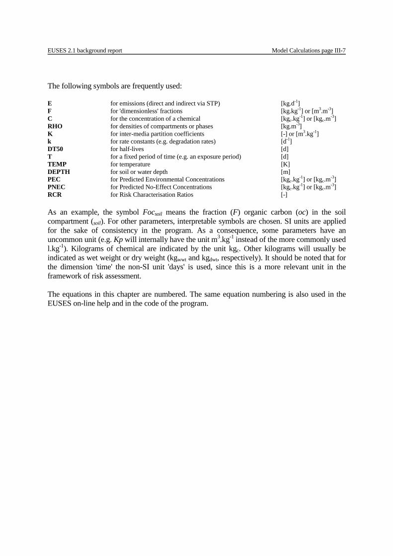
The following symbols are frequently used: E for emissions (direct and indirect via STP) [kg.d-1] F for 'dimensionless' fractions [kg.kg-1] or [m3.m-3] C for the concentration of a chemical [kgc.kg-1] or [kgc.m-3] RHO for densities of compartments or phases [kg.m-3] K for inter-media partition coefficients [-] or [m3.kg-1] k for rate constants (e.g. degradation rates) [d-1] DT50 for half-lives [d] T for a fixed period of time (e.g. an exposure period) [d] TEMP for temperature [K] DEPTH for soil or water depth [m] PEC for Predicted Environmental Concentrations [kgc.kg-1] or [kgc.m-3] PNEC for Predicted No-Effect Concentrations [kgc.kg-1] or [kgc.m-3] RCR for Risk Characterisation Ratios [-] As an example, the symbol Focsoil means the fraction (F) organic carbon (oc) in the soil compartment (soil). For other parameters, interpretable symbols are chosen. SI units are applied for the sake of consistency in the program. As a consequence, some parameters have an uncommon unit (e.g. Kp will internally have the unit m3.kg-1 instead of the more commonly used l.kg-1). Kilograms of chemical are indicated by the unit kgc. Other kilograms will usually be indicated as wet weight or dry weight (kgwwt and kgdwt, respectively). It should be noted that for the dimension 'time' the non-SI unit 'days' is used, since this is a more relevant unit in the framework of risk assessment. The equations in this chapter are numbered. The same equation numbering is also used in the EUSES on-line help and in the code of the program.
Model Calculations page III-8 EUSES 2.1 background report
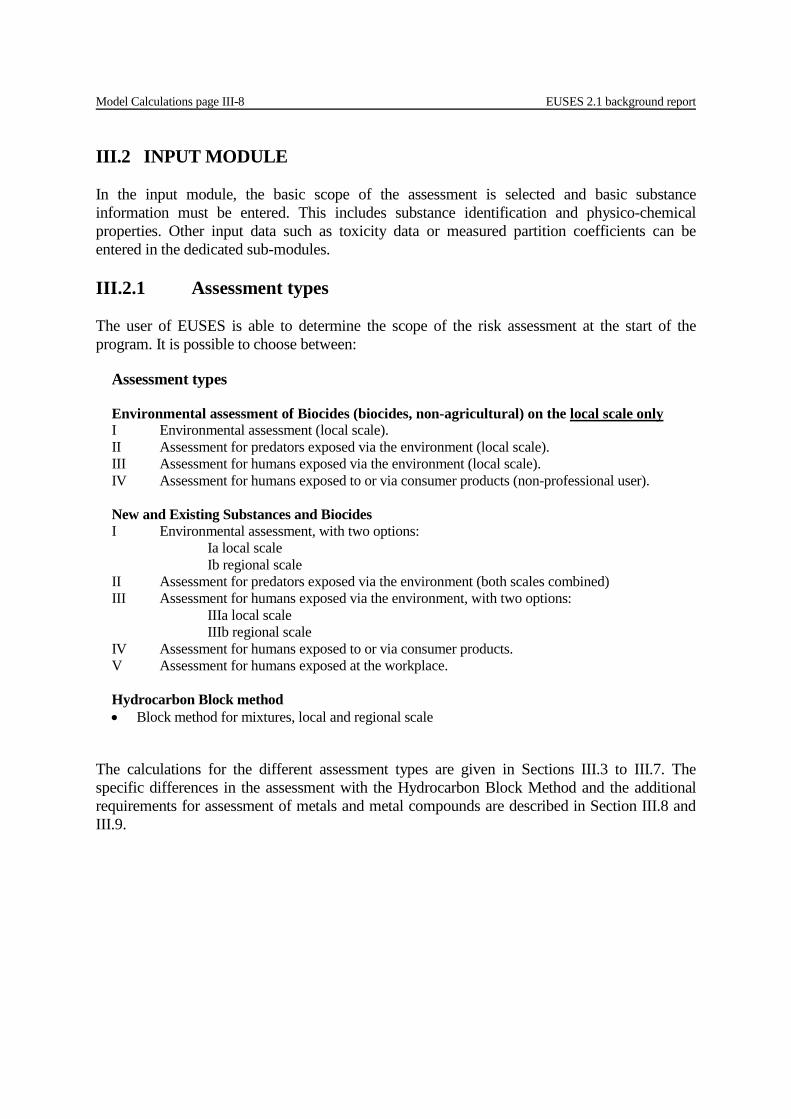
III.2 INPUT MODULE In the input module, the basic scope of the assessment is selected and basic substance information must be entered. This includes substance identification and physico-chemical properties. Other input data such as toxicity data or measured partition coefficients can be entered in the dedicated sub-modules. III.2.1 Assessment types The user of EUSES is able to determine the scope of the risk assessment at the start of the program. It is possible to choose between:
The calculations for the different assessment types are given in Sections III.3 to III.7. The specific differences in the assessment with the Hydrocarbon Block Method and the additional requirements for assessment of metals and metal compounds are described in Section III.8 and III.9.
Assessment types Environmental assessment of Biocides (biocides, non-agricultural) on the local scale only I Environmental assessment (local scale). II Assessment for predators exposed via the environment (local scale). III Assessment for humans exposed via the environment (local scale). IV Assessment for humans exposed to or via consumer products (non-professional user). New and Existing Substances and Biocides I Environmental assessment, with two options: Ia local scale Ib regional scale II Assessment for predators exposed via the environment (both scales combined) III Assessment for humans exposed via the environment, with two options: IIIa local scale IIIb regional scale IV Assessment for humans exposed to or via consumer products. V Assessment for humans exposed at the workplace. Hydrocarbon Block method • Block method for mixtures, local and regional scale
EUSES 2.1 background report Model Calculations page III-9
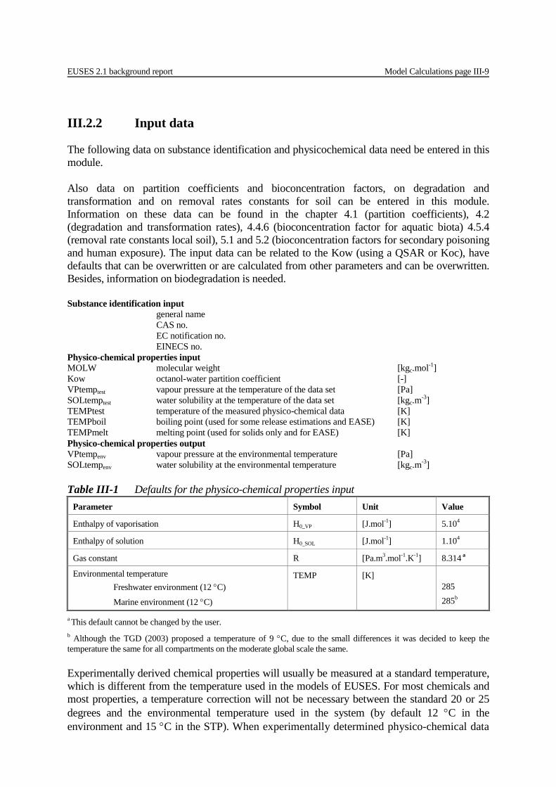
III.2.2 Input data The following data on substance identification and physicochemical data need be entered in this module. Also data on partition coefficients and bioconcentration factors, on degradation and transformation and on removal rates constants for soil can be entered in this module. Information on these data can be found in the chapter 4.1 (partition coefficients), 4.2 (degradation and transformation rates), 4.4.6 (bioconcentration factor for aquatic biota) 4.5.4 (removal rate constants local soil), 5.1 and 5.2 (bioconcentration factors for secondary poisoning and human exposure). The input data can be related to the Kow (using a QSAR or Koc), have defaults that can be overwritten or are calculated from other parameters and can be overwritten. Besides, information on biodegradation is needed. Substance identification input general name CAS no. EC notification no. EINECS no. Physico-chemical properties input MOLW molecular weight [kgc.mol-1] Kow octanol-water partition coefficient [-] VPtemptest vapour pressure at the temperature of the data set [Pa] SOLtemptest water solubility at the temperature of the data set [kgc.m-3] TEMPtest temperature of the measured physico-chemical data [K] TEMPboil boiling point (used for some release estimations and EASE) [K] TEMPmelt melting point (used for solids only and for EASE) [K] Physico-chemical properties output VPtempenv vapour pressure at the environmental temperature [Pa] SOLtempenv water solubility at the environmental temperature [kgc.m-3] Table III-1 Defaults for the physico-chemical properties input
Parameter Symbol Unit Value
Enthalpy of vaporisation H0_VP [J.mol-1] 5.104
Enthalpy of solution H0_SOL [J.mol-1] 1.104
Gas constant R [Pa.m3.mol-1.K-1] 8.314 a
Environmental temperature Freshwater environment (12 °C)
Marine environment (12 °C)
TEMP [K] 285 285b
a This default cannot be changed by the user. b Although the TGD (2003) proposed a temperature of 9 °C, due to the small differences it was decided to keep the temperature the same for all compartments on the moderate global scale the same. Experimentally derived chemical properties will usually be measured at a standard temperature, which is different from the temperature used in the models of EUSES. For most chemicals and most properties, a temperature correction will not be necessary between the standard 20 or 25 degrees and the environmental temperature used in the system (by default 12 °C in the environment and 15 °C in the STP). When experimentally determined physico-chemical data
Model Calculations page III-10 EUSES 2.1 background report
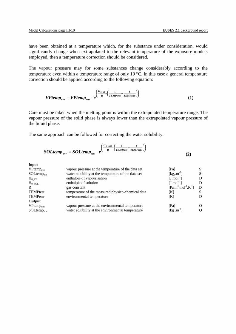
have been obtained at a temperature which, for the substance under consideration, would significantly change when extrapolated to the relevant temperature of the exposure models employed, then a temperature correction should be considered. The vapour pressure may for some substances change considerably according to the temperature even within a temperature range of only 10 °C. In this case a general temperature correction should be applied according to the following equation:
Care must be taken when the melting point is within the extrapolated temperature range. The vapour pressure of the solid phase is always lower than the extrapolated vapour pressure of the liquid phase. The same approach can be followed for correcting the water solubility:
−⋅
⋅ TEMPenvTEMPtestRH
testenv
SOL
e SOLtemp= SOLtemp11_0
(2) Input VPtemptest vapour pressure at the temperature of the data set [Pa] S SOLtemptest water solubility at the temperature of the data set [kgc.m-3] S H0_VP enthalpie of vapourisation [J.mol-1] D H0_SOL enthalpie of solution [J.mol-1] D R gas constant [Pa.m3.mol-1.K-1] D TEMPtest temperature of the measured physico-chemical data [K] S TEMPenv environmental temperature [K] D Output VPtempenv vapour pressure at the environmental temperature [Pa] O SOLtempenv water solubility at the environmental temperature [kgc.m-3] O
−⋅
⋅ TEMPenvTEMPtestRH
testenv
VP
e VPtemp= VPtemp11_0
(1)
EUSES 2.1 background report Model Calculations page III-11
III.3 RELEASE ESTIMATION FOR NEW AND EXISTING SUBSTANCES AND BIOCIDES
Releases to all spatial scales are estimated, based on use pattern and substance properties. The tables in Appendix III provide default release estimates for each category of substance. Release estimation applies either the tonnage of the substance as a starting point or representative dimensions (quantities, concentrations, etc.) for the process or the average consumption. In both cases emission factors (fractions released to the relevant environmental compartments) are used. These emission factors have been collected in the A-tables of Appendix III. In the TGD the A-tables the (realistic) worst case estimates are based on expert judgement and in some cases on use category documents. In this version of EUSES the emission factors of specific emission scenario documents of the TGD have been incorporated. The B-tables of the TGD contain data to determine the estimates for the daily quantity applicable for each relevant stage of the life cycle based on the tonnage. In this version of EUSES specific data on representative source size of the emission scenario documents of the TGD have been incorporated as well. It should be noted that release estimation using average capacities or consumption concerns the local scale only. For the regional scale an "overall" emission factor should be used.
Model Calculations page III-12 EUSES 2.1 background report
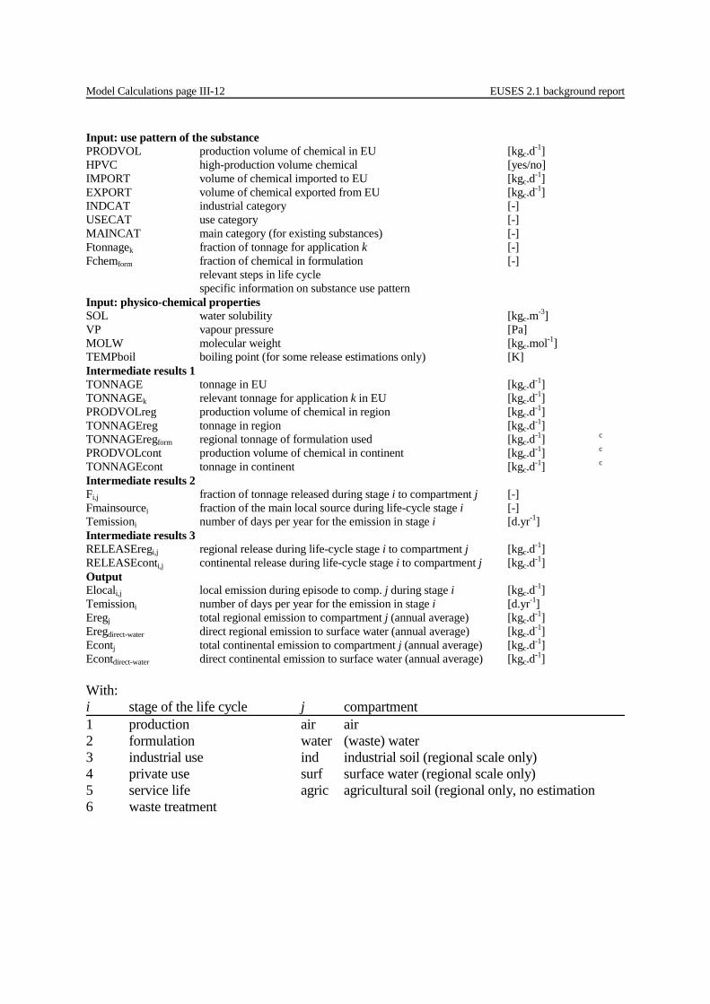
Input: use pattern of the substance PRODVOL production volume of chemical in EU [kgc.d-1] HPVC high-production volume chemical [yes/no] IMPORT volume of chemical imported to EU [kgc.d-1] EXPORT volume of chemical exported from EU [kgc.d-1] INDCAT industrial category [-] USECAT use category [-] MAINCAT main category (for existing substances) [-] Ftonnagek fraction of tonnage for application k [-] Fchemform fraction of chemical in formulation [-] relevant steps in life cycle specific information on substance use pattern Input: physico-chemical properties SOL water solubility [kgc.m-3] VP vapour pressure [Pa] MOLW molecular weight [kgc.mol-1] TEMPboil boiling point (for some release estimations only) [K] Intermediate results 1 TONNAGE tonnage in EU [kgc.d-1] TONNAGEk relevant tonnage for application k in EU [kgc.d-1] PRODVOLreg production volume of chemical in region [kgc.d-1] TONNAGEreg tonnage in region [kgc.d-1] TONNAGEregform regional tonnage of formulation used [kgc.d-1] c PRODVOLcont production volume of chemical in continent [kgc.d-1] c TONNAGEcont tonnage in continent [kgc.d-1] c Intermediate results 2 Fi,j fraction of tonnage released during stage i to compartment j [-] Fmainsourcei fraction of the main local source during life-cycle stage i [-] Temissioni number of days per year for the emission in stage i [d.yr-1] Intermediate results 3 RELEASEregi,j regional release during life-cycle stage i to compartment j [kgc.d-1] RELEASEconti,j continental release during life-cycle stage i to compartment j [kgc.d-1] Output Elocali,j local emission during episode to comp. j during stage i [kgc.d-1] Temissioni number of days per year for the emission in stage i [d.yr-1] Eregj total regional emission to compartment j (annual average) [kgc.d-1] Eregdirect-water direct regional emission to surface water (annual average) [kgc.d-1] Econtj total continental emission to compartment j (annual average) [kgc.d-1] Econtdirect-water direct continental emission to surface water (annual average) [kgc.d-1] With: i stage of the life cycle j compartment 1 production air air 2 formulation water (waste) water 3 industrial use ind industrial soil (regional scale only) 4 private use surf surface water (regional scale only) 5 service life agric agricultural soil (regional only, no estimation 6 waste treatment

EUSES 2.1 background report Model Calculations page III-13
III.3.1 Calculation of the tonnage of substance The total production volume in the EU is available in the data set and denoted by PRODVOL. TONNAGE is the volume of substance that is used for subsequent life-cycle stages.
Input PRODVOL production volume of chemical in EU [kgc.d-1] S IMPORT volume of chemical imported to EU [kgc.d-1] S EXPORT volume of chemical exported from EU [kgc.d-1] S Output TONNAGE tonnage of substance in EU [kgc.d-1] O When a substance has more than one application, the tonnage must be broken down for the different, relevant applications (indicated by the index k). Each application has a different combination of industrial and use category (INDCAT/USECAT).
Input TONNAGE total tonnage of substance in EU [kgc.d-1] O Ftonnagek fraction of total tonnage for application k [-] S Output TONNAGEk relevant tonnage for application k in EU [kgc.d-1] O This also implies that all parameters depending on the tonnage should also receive a subscript k (e.g. releases, environmental concentrations, risk characterisation ratios). This is not shown in this rest of this documentation. It should be noted that the production volume is not broken up according to this fraction since a chemical is usually produced according to one production method (independent of subsequent usages). In the program, production can be set to 'relevant' for more than one usage. In that case, each production stage can be calculated with the relevant percentage of the total production volume. If application k concerns a biocide the life cycle stages concerning the application – such as industrial use – have to be evaluated separately (see section III.2.1. Assessment types). This can
Table III-2 Defaults for emission calculations. Parameter Symbol Unit Value
Fraction of EU production volume of substance produced in the region
Fprodvolreg [-] 1 a
Fraction connected to sewer systems Fconnectstp [-] 0.80
a For life cycle stage Private use the default remains 0.10.
EXPORT -IMPORT + PRODVOL= TONNAGE (3)
TONNAGEFtonnageTONNAGE kk ⋅= (4)
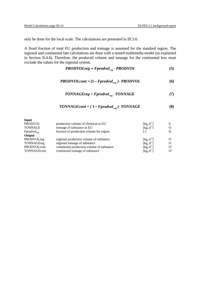
Model Calculations page III-14 EUSES 2.1 background report
only be done for the local scale. The calculations are presented in III.3.6. A fixed fraction of total EU production and tonnage is assumed for the standard region. The regional and continental fate calculations are done with a nested multimedia model (as explained in Section II.4.4). Therefore, the produced volume and tonnage for the continental box must exclude the values for the regional system.
Input PRODVOL production volume of chemical in EU [kgc.d-1] S TONNAGE tonnage of substance in EU [kgc.d-1] O Fprodvolreg fraction of production volume for region [-] D Output PRODVOLreg regional production volume of substance [kgc.d-1] O TONNAGEreg regional tonnage of substance [kgc.d-1] O PRODVOLcont continental production volume of substance [kgc.d-1] Oc TONNAGEcont continental tonnage of substance [kgc.d-1] Oc
PRODVOLFprodvolPRODVOLreg reg ⋅= (5)
PRODVOL )Fprodvol= tPRODVOLcon reg ⋅−1( (6)
TONNAGE Fprodvol= TONNAGEreg reg ⋅ (7)
TONNAGE )Fprodvol (= tTONNAGEcon reg ⋅−1 (8)
EUSES 2.1 background report Model Calculations page III-15
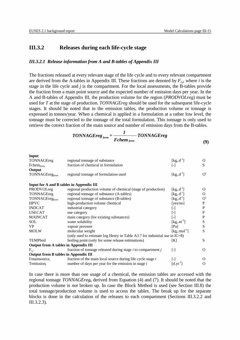
III.3.2 Releases during each life-cycle stage
III.3.2.1 Release information from A and B-tables of Appendix III The fractions released at every relevant stage of the life cycle and to every relevant compartment are derived from the A-tables in Appendix III. These fractions are denoted by Fi,j, where i is the stage in the life cycle and j is the compartment. For the local assessments, the B-tables provide the fraction from a main point source and the expected number of emission days per year. In the A and B-tables of Appendix III, the production volume for the region (PRODVOLreg) must be used for T at the stage of production. TONNAGEreg should be used for the subsequent life-cycle stages. It should be noted that in the emission tables, the production volume or tonnage is expressed in tonnes/year. When a chemical is applied in a formulation at a rather low level, the tonnage must be corrected to the tonnage of the total formulation. This tonnage is only used to retrieve the correct fraction of the main source and number of emission days from the B-tables.
Input TONNAGEreg regional tonnage of substance [kgc.d-1] O Fchemform fraction of chemical in formulation [-] S Output TONNAGEregform regional tonnage of formulation used [kgc.d-1] Oc Input for A and B tables in Appendix III PRODVOLreg regional production volume of chemical (stage of production) [kgc.d-1] O TONNAGEreg regional tonnage of substance (A-tables) [kgc.d-1] O TONNAGEregform regional tonnage of substance (B-tables) [kgc.d-1] Oc HPVC high-production volume chemical [yes/no] P INDCAT industrial category [-] P USECAT use category [-] P MAINCAT main category (for existing substances) [-] P SOL water solubility [kgc.m-3] S VP vapour pressure [Pa] S MOLW molecular weight [kgc.mol-1] S (only used to estimate log Henry in Table A3.7 for industrial use in IC=8) TEMPboil boiling point (only for some release estimations) [K] S Output from A tables in Appendix III Fi,j fraction of tonnage released during stage i to compartment j [-] O Output from B tables in Appendix III Fmainsourcei fraction of the main local source during life cycle stage i [-] O Temissioni number of days per year for the emission in stage i [d.yr-1] O In case there is more than one usage of a chemical, the emission tables are accessed with the regional tonnage TONNAGEregk derived from Equation (4) and (7). It should be noted that the production volume is not broken up. In case the Block Method is used (see Section III.8) the total tonnage/production volume is used to access the tables. The break up for the separate blocks is done in the calculation of the releases to each compartment (Sections III.3.2.2 and III.3.2.3).
TONNAGEreg
Fchem1= TONNAGEreg
formform ⋅
(9)

Model Calculations page III-16 EUSES 2.1 background report
III.3.2.2 Continental releases The annual average release per stage of the life cycle can be calculated with the following series of equations. For each relevant stage, the losses in the previous stage are taken into account. Note that releases during production are not taken into account in the other stages, as these releases will generally already be accounted for in the reported production volume. 1. production RELEASEcont1,j : air F1, air ⋅ PRODVOLcont water F1, water ⋅ PRODVOLcont soil F1, ind ⋅ PRODVOLcont surf F1, surf ⋅ PRODVOLcont total ΣF1, j ⋅ PRODVOLcont amount used: TONNAGEcont 2. formulation RELEASEcont2,j : air F2, air ⋅ TONNAGEcont water F2, water ⋅ TONNAGEcont soil F2, ind ⋅ TONNAGEcont surf F2, surf ⋅ TONNAGEcont total ΣF2, j ⋅ TONNAGEcont rest: (1-ΣF2, j ) ⋅TONNAGEcont 3. industrial use RELEASEcont3,j : air F3, air ⋅ (1-ΣF2, j) ⋅TONNAGEcont water F3, water ⋅ (1-ΣF2, j ) ⋅ TONNAGEcont soil F3, ind ⋅ (1-ΣF2, j ) ⋅ TONNAGEcont surf F3, surf ⋅ (1-ΣF2, j ) ⋅ TONNAGEcont total ΣF3, j ⋅ (1-ΣF2, j ) ⋅ TONNAGEcont 4. private use RELEASEcont4,j : air F4, air ⋅ (1-ΣF2, j ) ⋅ TONNAGEcont water F4, water ⋅ (1-ΣF2, j ) ⋅ TONNAGEcont soil F4, ind ⋅ (1-ΣF2, j ) ⋅ TONNAGEcont surf F4, surf ⋅ (1-ΣF2, j ) ⋅ TONNAGEcont total ΣF4, j ⋅ (1-ΣF2, j ) ⋅ TONNAGEcont rest: (1-ΣF3, j - ΣF4, j ) ⋅ (1-ΣF2,j ) ⋅ TONNAGEcont 5. service life RELEASEcont5,j : air F5, air ⋅ (1-ΣF3, j - ΣF4, j ) ⋅ (1-ΣF2,j ) ⋅ TONNAGEcont water F5, water ⋅ (1-ΣF3, j - ΣF4, j ) ⋅ (1-ΣF2,j ) ⋅ TONNAGEcont soil F5, ind ⋅ (1-ΣF3, j - ΣF4, j ) ⋅ (1-ΣF2,j ) ⋅ TONNAGEcont surf F5, surf ⋅ (1-ΣF3, j - ΣF4, j ) ⋅ (1-ΣF2,j ) ⋅ TONNAGEcont total ΣF5, j ⋅ (1-ΣF3, j - ΣF4, j ) ⋅ (1-ΣF2,j ) ⋅ TONNAGEcont
EUSES 2.1 background report Model Calculations page III-17
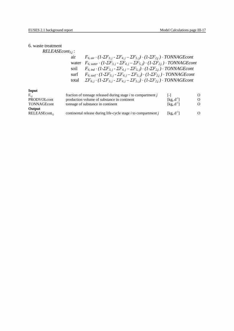
6. waste treatment RELEASEcont5,j : air F6, air ⋅ (1-ΣF3, j - ΣF4, j – ΣF5, j) ⋅ (1-ΣF2,j ) ⋅ TONNAGEcont water F6, water ⋅ (1-ΣF3, j - ΣF4, j – ΣF5, j) ⋅ (1-ΣF2,j ) ⋅ TONNAGEcont soil F6, ind ⋅ (1-ΣF3, j - ΣF4, j – ΣF5, j) ⋅ (1-ΣF2,j ) ⋅ TONNAGEcont surf F6, surf ⋅ (1-ΣF3, j - ΣF4, j – ΣF5, j) ⋅ (1-ΣF2,j ) ⋅ TONNAGEcont total ΣF6, j ⋅ (1-ΣF3, j - ΣF4, j – ΣF5, j) ⋅ (1-ΣF2,j ) ⋅ TONNAGEcont Input Fi,j fraction of tonnage released during stage i to compartment j [-] O PRODVOLcont production volume of substance in continent [kgc.d-1] O TONNAGEcont tonnage of substance in continent [kgc.d-1] O Output RELEASEconti,j continental release during life-cycle stage i to compartment j [kgc.d-1] O
Model Calculations page III-18 EUSES 2.1 background report
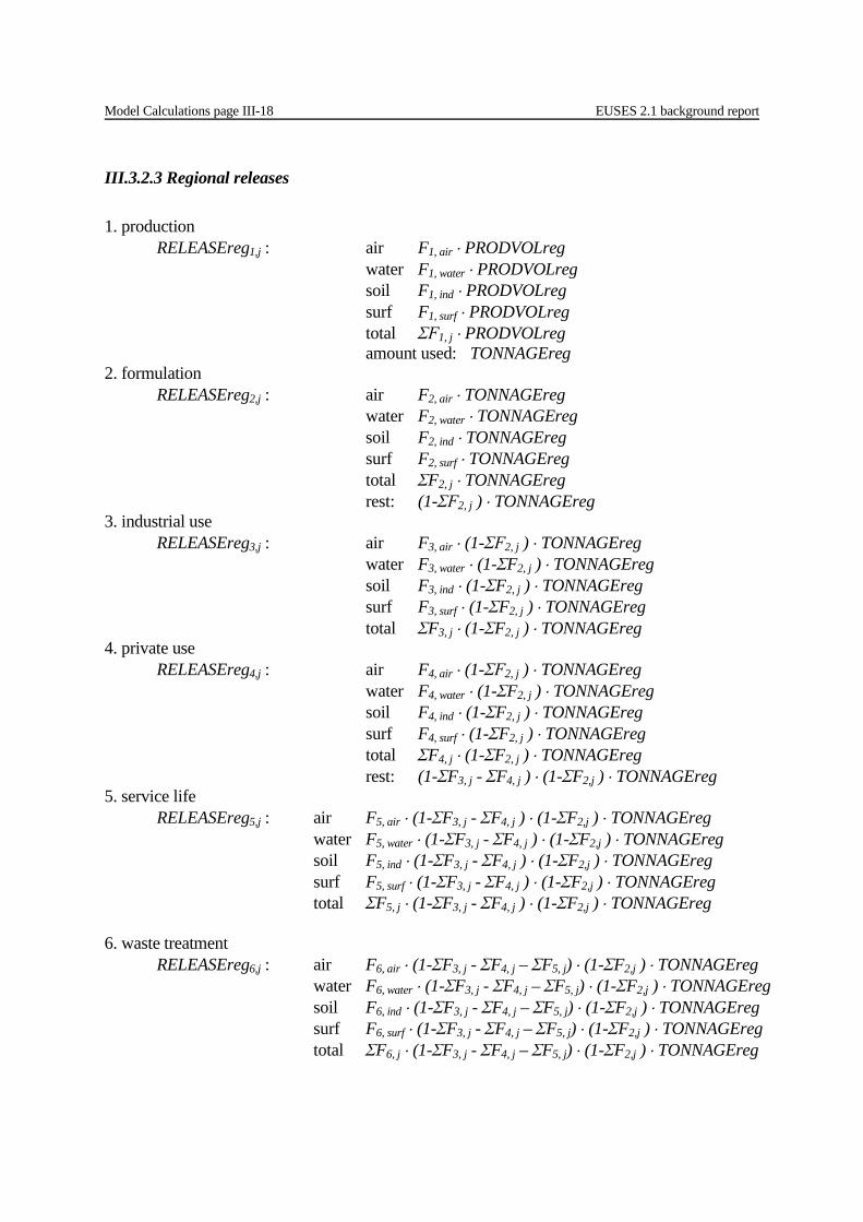
III.3.2.3 Regional releases 1. production RELEASEreg1,j : air F1, air ⋅ PRODVOLreg water F1, water ⋅ PRODVOLreg soil F1, ind ⋅ PRODVOLreg surf F1, surf ⋅ PRODVOLreg total ΣF1, j ⋅ PRODVOLreg amount used: TONNAGEreg 2. formulation RELEASEreg2,j : air F2, air ⋅ TONNAGEreg water F2, water ⋅ TONNAGEreg soil F2, ind ⋅ TONNAGEreg surf F2, surf ⋅ TONNAGEreg total ΣF2, j ⋅ TONNAGEreg rest: (1-ΣF2, j ) ⋅ TONNAGEreg 3. industrial use RELEASEreg3,j : air F3, air ⋅ (1-ΣF2, j ) ⋅ TONNAGEreg water F3, water ⋅ (1-ΣF2, j ) ⋅ TONNAGEreg soil F3, ind ⋅ (1-ΣF2, j ) ⋅ TONNAGEreg surf F3, surf ⋅ (1-ΣF2, j ) ⋅ TONNAGEreg total ΣF3, j ⋅ (1-ΣF2, j ) ⋅ TONNAGEreg 4. private use RELEASEreg4,j : air F4, air ⋅ (1-ΣF2, j ) ⋅ TONNAGEreg water F4, water ⋅ (1-ΣF2, j ) ⋅ TONNAGEreg soil F4, ind ⋅ (1-ΣF2, j ) ⋅ TONNAGEreg surf F4, surf ⋅ (1-ΣF2, j ) ⋅ TONNAGEreg total ΣF4, j ⋅ (1-ΣF2, j ) ⋅ TONNAGEreg rest: (1-ΣF3, j - ΣF4, j ) ⋅ (1-ΣF2,j ) ⋅ TONNAGEreg 5. service life RELEASEreg5,j : air F5, air ⋅ (1-ΣF3, j - ΣF4, j ) ⋅ (1-ΣF2,j ) ⋅ TONNAGEreg water F5, water ⋅ (1-ΣF3, j - ΣF4, j ) ⋅ (1-ΣF2,j ) ⋅ TONNAGEreg soil F5, ind ⋅ (1-ΣF3, j - ΣF4, j ) ⋅ (1-ΣF2,j ) ⋅ TONNAGEreg surf F5, surf ⋅ (1-ΣF3, j - ΣF4, j ) ⋅ (1-ΣF2,j ) ⋅ TONNAGEreg total ΣF5, j ⋅ (1-ΣF3, j - ΣF4, j ) ⋅ (1-ΣF2,j ) ⋅ TONNAGEreg 6. waste treatment RELEASEreg6,j : air F6, air ⋅ (1-ΣF3, j - ΣF4, j – ΣF5, j) ⋅ (1-ΣF2,j ) ⋅ TONNAGEreg water F6, water ⋅ (1-ΣF3, j - ΣF4, j – ΣF5, j) ⋅ (1-ΣF2,j ) ⋅ TONNAGEreg soil F6, ind ⋅ (1-ΣF3, j - ΣF4, j – ΣF5, j) ⋅ (1-ΣF2,j ) ⋅ TONNAGEreg surf F6, surf ⋅ (1-ΣF3, j - ΣF4, j – ΣF5, j) ⋅ (1-ΣF2,j ) ⋅ TONNAGEreg total ΣF6, j ⋅ (1-ΣF3, j - ΣF4, j – ΣF5, j) ⋅ (1-ΣF2,j ) ⋅ TONNAGEreg

EUSES 2.1 background report Model Calculations page III-19
Input Fi,j fraction of tonnage released during stage i to compartment j [-] O PRODVOLreg regional production volume of substance [kgc.d-1] O TONNAGEreg regional tonnage of substance [kgc.d-1] O Output RELEASEregi,j regional release during life-cycle stage i to compartment j [kgc.d-1] O
Model Calculations page III-20 EUSES 2.1 background report
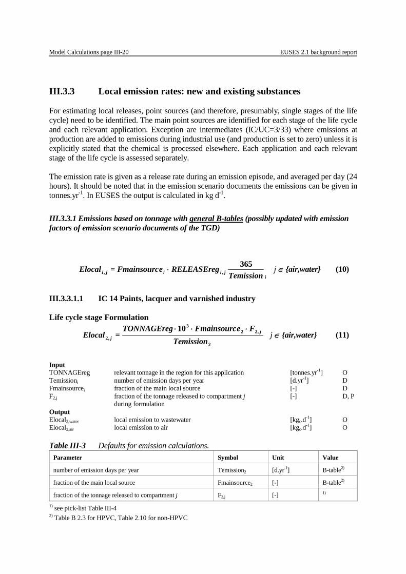
III.3.3 Local emission rates: new and existing substances For estimating local releases, point sources (and therefore, presumably, single stages of the life cycle) need to be identified. The main point sources are identified for each stage of the life cycle and each relevant application. Exception are intermediates (IC/UC=3/33) where emissions at production are added to emissions during industrial use (and production is set to zero) unless it is explicitly stated that the chemical is processed elsewhere. Each application and each relevant stage of the life cycle is assessed separately. The emission rate is given as a release rate during an emission episode, and averaged per day (24 hours). It should be noted that in the emission scenario documents the emissions can be given in tonnes.yr-1. In EUSES the output is calculated in kg d-1.
III.3.3.1 Emissions based on tonnage with general B-tables (possibly updated with emission factors of emission scenario documents of the TGD)
i
jiiji TemissionRELEASEregeFmainsourc=Elocal 365
,, ⋅ j ∈ {air,water} (10)
III.3.3.1.1 IC 14 Paints, lacquer and varnished industry Life cycle stage Formulation
2
,223
,2
10Temission
FeFmainsourcTONNAGEreg=Elocal j
j
⋅⋅⋅ j ∈ {air,water} (11)
Input TONNAGEreg relevant tonnage in the region for this application [tonnes.yr-1] O Temissioni number of emission days per year [d.yr-1] D Fmainsourcei fraction of the main local source [-] D F2,j fraction of the tonnage released to compartment j [-] D, P during formulation Output Elocal2,water local emission to wastewater [kgc.d-1] O Elocal2,air local emission to air [kgc.d-1] O Table III-3 Defaults for emission calculations.
Parameter Symbol Unit Value
number of emission days per year Temission2 [d.yr-1] B-table2)
fraction of the main local source Fmainsource2 [-] B-table2)
fraction of the tonnage released to compartment j F2,j [-] 1)
1) see pick-list Table III-4 2) Table B 2.3 for HPVC, Table 2.10 for non-HPVC
EUSES 2.1 background report Model Calculations page III-21
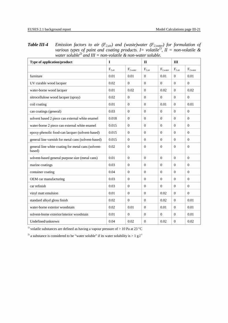
Table III-4 Emission factors to air (F2,air) and (waste)water (F2,water) for formulation of various types of paint and coating products. I= volatile1), II = non-volatile & water soluble2) and III = non-volatile & non-water soluble.
Type of application/product I II III
F2,air F2,water F2,air F2,water F2,air F2,water
furniture 0.01 0.01 0 0.01 0 0.01
UV curable wood lacquer 0.02 0 0 0 0 0
water-borne wood lacquer 0.01 0.02 0 0.02 0 0.02
nitrocellulose wood lacquer (spray) 0.02 0 0 0 0 0
coil coating 0.01 0 0 0.01 0 0.01
can coatings (general) 0.03 0 0 0 0 0
solvent based 2 piece can external white enamel 0.018 0 0 0 0 0
water-borne 2 piece can external white enamel 0.015 0 0 0 0 0
epoxy-phenolic food-can lacquer (solvent-based) 0.015 0 0 0 0 0
general line varnish for metal cans (solvent-based) 0.015 0 0 0 0 0
general line white coating for metal cans (solvent-based)
0.02 0 0 0 0 0
solvent-based general purpose size (metal cans) 0.01 0 0 0 0 0
marine coatings 0.03 0 0 0 0 0
container coating 0.04 0 0 0 0 0
OEM car manufacturing 0.03 0 0 0 0 0
car refinish 0.03 0 0 0 0 0
vinyl matt emulsion 0.01 0 0 0.02 0 0
standard alkyd gloss finish 0.02 0 0 0.02 0 0.01
water-borne exterior woodstain 0.02 0.01 0 0.01 0 0.01
solvent-borne exterior/interior woodstain 0.01 0 0 0 0 0.01
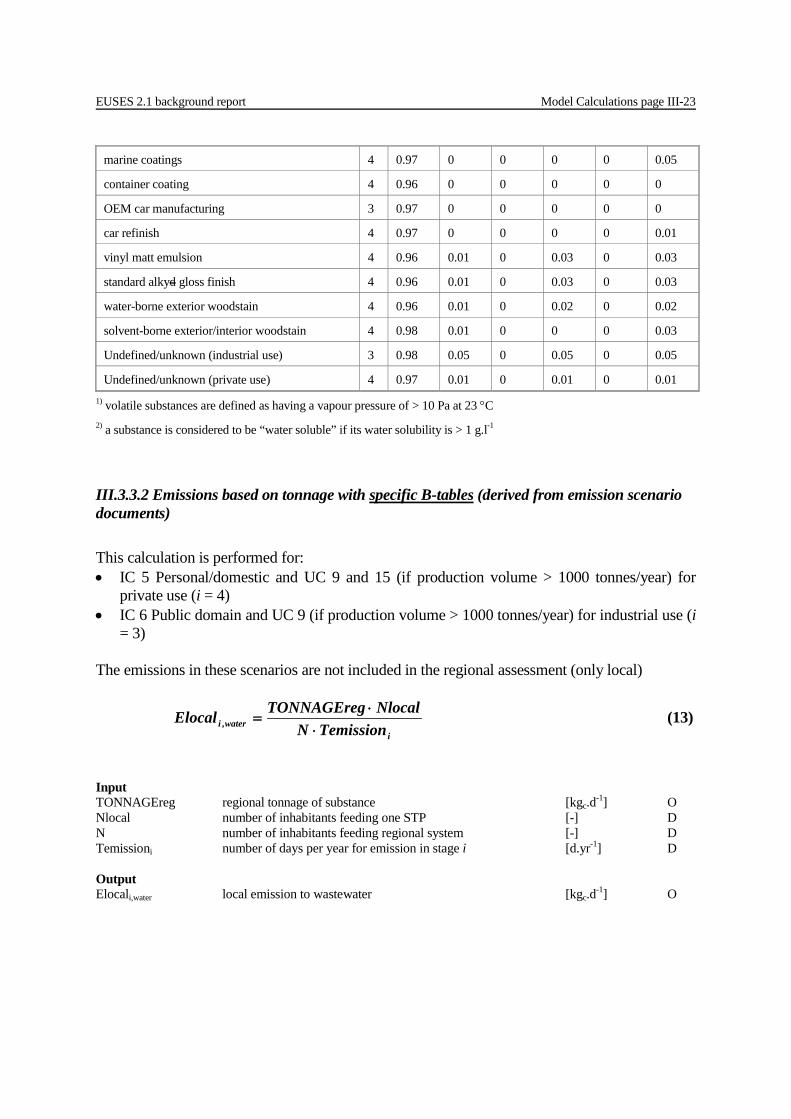
Undefined/unknown 0.04 0.02 0 0.02 0 0.02 1) volatile substances are defined as having a vapour pressure of > 10 Pa at 23 °C 2) a substance is considered to be “water soluble” if its water solubility is > 1 g.l-1

Model Calculations page III-22 EUSES 2.1 background report
Life cycle stage Industrial use (i=3) and Private use (i=4)
i
jiiji Temission
FeFmainsourcTONNAGEreg=Elocal ,
,
⋅⋅ j ∈ {air,water} (12)
Input TONNAGEreg relevant tonnage in the region for this application [kgc.yr-1] O Temissioni number of emission days per year [d.yr-1] D Fmainsourcei fraction of the main local source [-] D Fi,j fraction of the tonnage released to compartment j [-] D, P during life cycle stage i Output Elocali,water local emission to wastewater [kgc.d-1] O Elocali,air local emission to air [kgc.d-1] O Table III-5 Defaults for emission calculations.
Parameter Symbol Unit Value
number of emission days per year Temissioni [d.yr-1] B-table2)
fraction of the main local source Fmainsourcei [-] B-table2)
fraction of the tonnage released to compartment j Fi,j [-] 1)
1) see pick-list Table III-6 2) i = 3: Table B 3.13; i = 4: Table B 4.4 (for wastewater only) Table III-6 Emission factors to air (Fi, air) and (waste)water (Fi, water) for industrial use (i =
3) and private use (i = 4) of various types of paint and coating products. I= volatile1), II = non-volatile & water soluble2) and III = non-volatile & non-water soluble.
Type of applicate ion / product i I II III
Fi,air Fi,water Fi,air Fi,water Fi,air F2,water
Furniture 4 0.97 0.01 0 0.03 0 0.03
UV curable wood lacquer 4 0.98 0 0 0 0 0
water-borne wood lacquer 4 0.92 0.05 0 0.05 0 0.05
nitrocellulose wood lacquer (spray) 4 0.98 0 0 0 0 0
coil coating 3 0.01 0.01 0 0.01 0 0.01
can coatings (general) 3 0.94 0 0 0 0 0
solvent based 2 piece can external white enamel 3 0.96 0 0 0 0 0
water-borne 2 piece can external white enamel 3 0.965 0 0 0 0 0
epoxy-phenolic food-can lacquer (solvent-based) 3 0.93 0 0 0 0 0
general line varnish for metal cans (solvent-based)
3 0.934 0 0 0 0 0
general line white coating for metal cans (solvent-based)
3 0.927 0 0 0 0 0
solvent-based general purpose size (metal cans) 3 0.939 0 0 0 0 0
EUSES 2.1 background report Model Calculations page III-23
marine coatings 4 0.97 0 0 0 0 0.05
container coating 4 0.96 0 0 0 0 0
OEM car manufacturing 3 0.97 0 0 0 0 0
car refinish 4 0.97 0 0 0 0 0.01
vinyl matt emulsion 4 0.96 0.01 0 0.03 0 0.03
standard alkyd gloss finish 4 0.96 0.01 0 0.03 0 0.03
water-borne exterior woodstain 4 0.96 0.01 0 0.02 0 0.02
solvent-borne exterior/interior woodstain 4 0.98 0.01 0 0 0 0.03
Undefined/unknown (industrial use) 3 0.98 0.05 0 0.05 0 0.05
Undefined/unknown (private use) 4 0.97 0.01 0 0.01 0 0.01 1) volatile substances are defined as having a vapour pressure of > 10 Pa at 23 °C 2) a substance is considered to be “water soluble” if its water solubility is > 1 g.l-1
III.3.3.2 Emissions based on tonnage with specific B-tables (derived from emission scenario documents) This calculation is performed for: • IC 5 Personal/domestic and UC 9 and 15 (if production volume > 1000 tonnes/year) for
private use (i = 4) • IC 6 Public domain and UC 9 (if production volume > 1000 tonnes/year) for industrial use (i
= 3) The emissions in these scenarios are not included in the regional assessment (only local)
i
wateri TemissionNNlocalTONNAGEregElocal
⋅⋅
=, (13)
Input TONNAGEreg regional tonnage of substance [kgc.d-1] O Nlocal number of inhabitants feeding one STP [-] D N number of inhabitants feeding regional system [-] D Temissioni number of days per year for emission in stage i [d.yr-1] D Output Elocali,water local emission to wastewater [kgc.d-1] O
Model Calculations page III-24 EUSES 2.1 background report
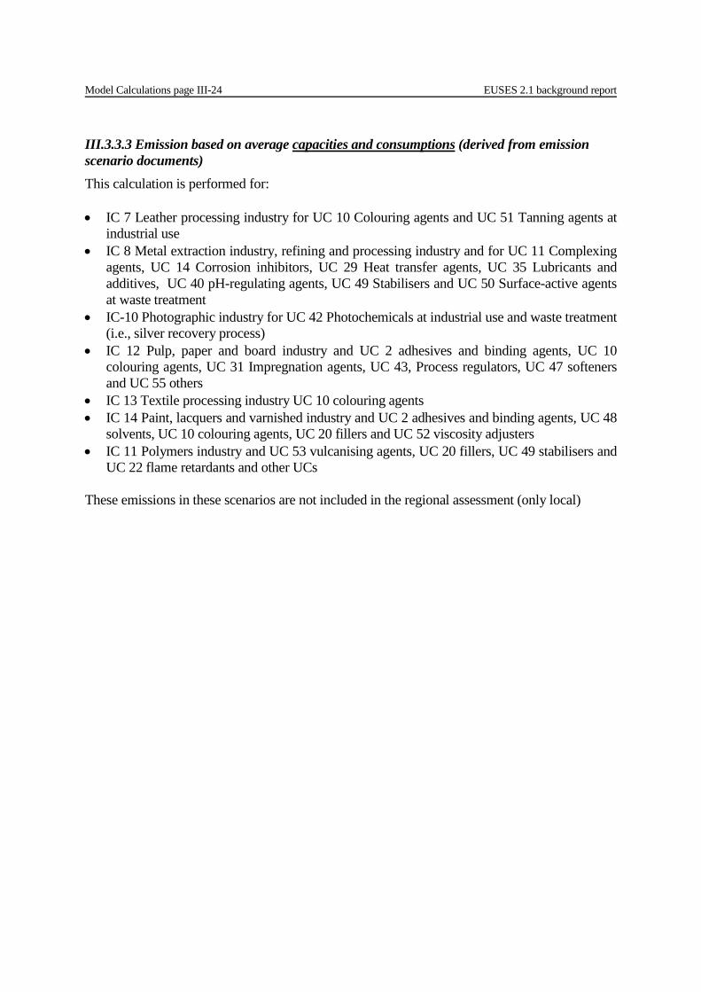
III.3.3.3 Emission based on average capacities and consumptions (derived from emission scenario documents) This calculation is performed for: • IC 7 Leather processing industry for UC 10 Colouring agents and UC 51 Tanning agents at
industrial use • IC 8 Metal extraction industry, refining and processing industry and for UC 11 Complexing
agents, UC 14 Corrosion inhibitors, UC 29 Heat transfer agents, UC 35 Lubricants and additives, UC 40 pH-regulating agents, UC 49 Stabilisers and UC 50 Surface-active agents at waste treatment
• IC-10 Photographic industry for UC 42 Photochemicals at industrial use and waste treatment (i.e., silver recovery process)
• IC 12 Pulp, paper and board industry and UC 2 adhesives and binding agents, UC 10 colouring agents, UC 31 Impregnation agents, UC 43, Process regulators, UC 47 softeners and UC 55 others
• IC 13 Textile processing industry UC 10 colouring agents • IC 14 Paint, lacquers and varnished industry and UC 2 adhesives and binding agents, UC 48
solvents, UC 10 colouring agents, UC 20 fillers and UC 52 viscosity adjusters • IC 11 Polymers industry and UC 53 vulcanising agents, UC 20 fillers, UC 49 stabilisers and
UC 22 flame retardants and other UCs These emissions in these scenarios are not included in the regional assessment (only local)
EUSES 2.1 background report Model Calculations page III-25
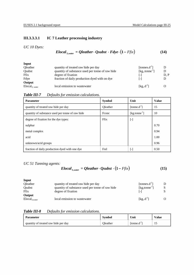
III.3.3.3.1 IC 7 Leather processing industry UC 10 Dyes: ( )Ffix−⋅⋅⋅ 1,3 Fdye Qsubst Qleather=Elocal water (14)
Input Qleather quantity of treated raw hide per day [tonnes.d-1] D Qsubst quantity of substance used per tonne of raw hide [kgc.tonne-1] D Ffix degree of fixation [-] D, P Fdye fraction of daily production dyed with on dye [-] D Output Elocal3, water local emission to wastewater [kgc.d-1] O Table III-7 Defaults for emission calculations.
Parameter Symbol Unit Value
quantity of treated raw hide per day Qleather [tonne.d-1] 15
quantity of substance used per tonne of raw hide Fconc [kg.tonne-1] 10
degree of fixation for the dye types:
sulphur
metal complex
acid
unknown/acid groups
Ffix [-]
0.70
0.94
1.00
0.96
fraction of daily production dyed with one dye Frel [-] 0.50
UC 51 Tanning agents: ( )Ffix−⋅⋅ 1,3 Qsubst Qleather=Elocal water (15)
Input Qleather quantity of treated raw hide per day [tonnes.d-1] D Qsubst quantity of substance used per tonne of raw hide [kgctonne-1] S Ffix degree of fixation [-] S Output Elocal3,water local emission to wastewater [kgc.d-1] O Table III-8 Defaults for emission calculations.
Parameter Symbol Unit Value
quantity of treated raw hide per day Qleather [tonne.d-1] 15
Model Calculations page III-26 EUSES 2.1 background report
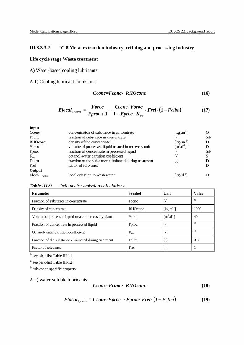
III.3.3.3.2 IC 8 Metal extraction industry, refining and processing industry Life cycle stage Waste treatment A) Water-based cooling lubricants A.1) Cooling lubricant emulsions: RHOconccCconc=Fcon ⋅ (16)
( )Felim−⋅⋅⋅+
⋅⋅
+1
11,6 FrelKFproc
VprocCconc Fproc
Fproc=Elocalow
water (17)
Input Cconc concentration of substance in concentrate [kgc.m-3] O Fconc fraction of substance in concentrate [-] S/P RHOconc density of the concentrate [kgc.m-3] D Vproc volume of processed liquid treated in recovery unit [m3.d-1] D Fproc fraction of concentrate in processed liquid [-] S/P Kow octanol-water partition coefficient [-] S Felim fraction of the substance eliminated during treatment [-] D Frel factor of relevance [-] D Output Elocal6, water local emission to wastewater [kgc.d-1] O Table III-9 Defaults for emission calculations.
Parameter Symbol Unit Value
Fraction of substance in concentrate Fconc [-] 1)
Density of concentrate RHOconc [kg.m-3] 1000
Volume of processed liquid treated in recovery plant Vproc [m3.d-1] 40
Fraction of concentrate in processed liquid Fproc [-] 2)
Octanol-water partition coefficient Kow [-] 3)
Fraction of the substance eliminated during treatment Felim [-] 0.8
Factor of relevance Frel [-] 1 1) see pick-list Table III-11 2) see pick-list Table III-12 3) substance specific property A.2) water-soluble lubricants: RHOconccCconc=Fcon ⋅ (18)
( )Felim−⋅⋅⋅⋅ 1FrelFprocVproc Cconc=Elocal water,6 (19)
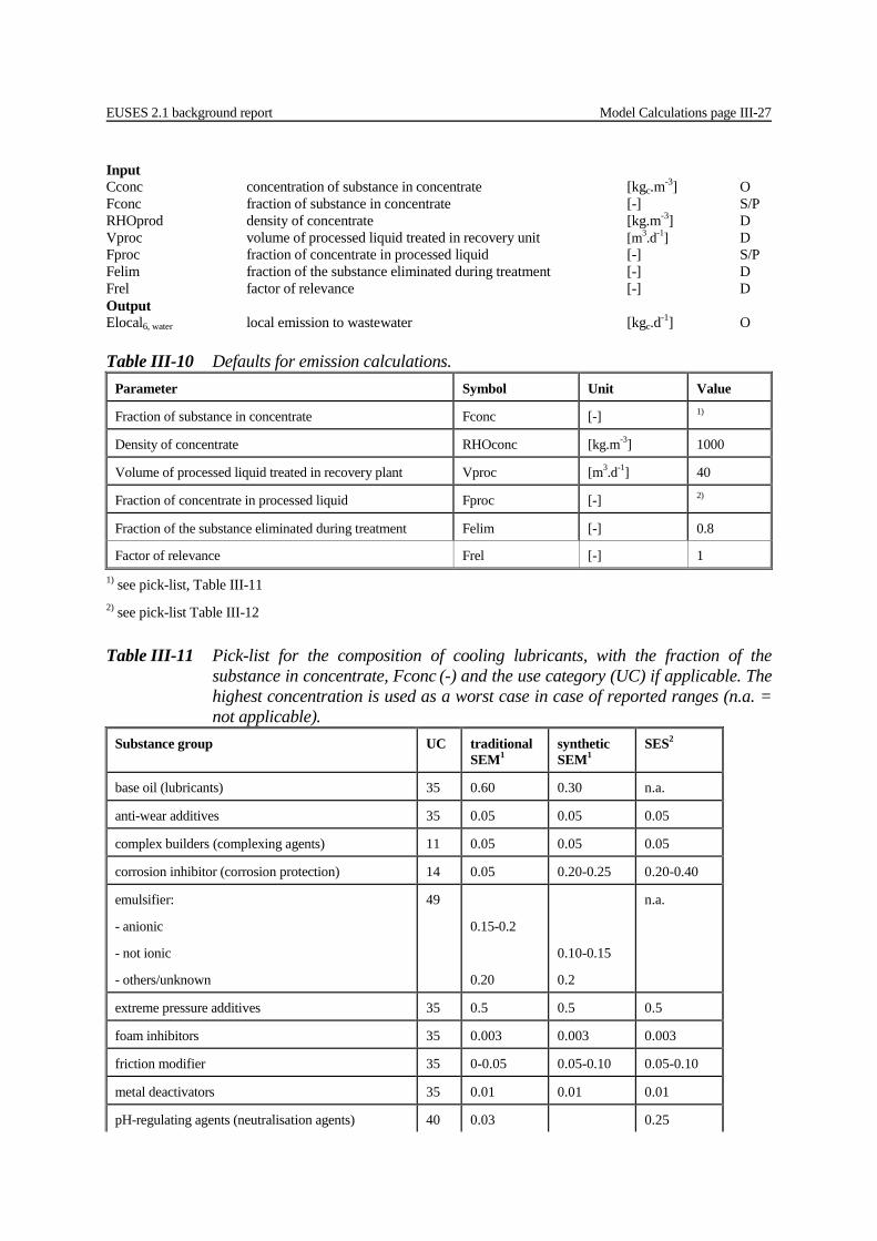
EUSES 2.1 background report Model Calculations page III-27
Input Cconc concentration of substance in concentrate [kgc.m-3] O Fconc fraction of substance in concentrate [-] S/P RHOprod density of concentrate [kg.m-3] D Vproc volume of processed liquid treated in recovery unit [m3.d-1] D Fproc fraction of concentrate in processed liquid [-] S/P Felim fraction of the substance eliminated during treatment [-] D Frel factor of relevance [-] D Output Elocal6, water local emission to wastewater [kgc.d-1] O Table III-10 Defaults for emission calculations.
Parameter Symbol Unit Value
Fraction of substance in concentrate Fconc [-] 1)
Density of concentrate RHOconc [kg.m-3] 1000
Volume of processed liquid treated in recovery plant Vproc [m3.d-1] 40
Fraction of concentrate in processed liquid Fproc [-] 2)
Fraction of the substance eliminated during treatment Felim [-] 0.8
Factor of relevance Frel [-] 1 1) see pick-list, Table III-11 2) see pick-list Table III-12 Table III-11 Pick-list for the composition of cooling lubricants, with the fraction of the
substance in concentrate, Fconc (-) and the use category (UC) if applicable. The highest concentration is used as a worst case in case of reported ranges (n.a. = not applicable).
Substance group UC traditional SEM1
synthetic SEM1
SES2
base oil (lubricants) 35 0.60 0.30 n.a.
anti-wear additives 35 0.05 0.05 0.05
complex builders (complexing agents) 11 0.05 0.05 0.05
corrosion inhibitor (corrosion protection) 14 0.05 0.20-0.25 0.20-0.40
emulsifier:
- anionic
- not ionic
- others/unknown
49
0.15-0.2
0.20
0.10-0.15
0.2
n.a.
extreme pressure additives 35 0.5 0.5 0.5
foam inhibitors 35 0.003 0.003 0.003
friction modifier 35 0-0.05 0.05-0.10 0.05-0.10
metal deactivators 35 0.01 0.01 0.01
pH-regulating agents (neutralisation agents) 40 0.03 0.25

Model Calculations page III-28 EUSES 2.1 background report
solubilisers 35 0.05 0.05 0.10-0.20
surfactants:
- anionic surfactants
- others/unknown
50
0.25
0.25
0.25
0.25
0.25
0.25 1) SEM emulsifiable cooling lubricant 2) SES water soluble cooling lubricant
Table III-12 Pick-list for fraction of cooling lubricant concentrate in processed liquid, Fproc
(-) by type of process. The highest concentration is used as a worst case when ranges are reported.
Process Fproc Broaching 0.10-0.20
thread cutting 0.05-0.10
deep hole drilling 0.10-0.20
parting-off 0.05-0.10
milling, cylindrical milling 0.05-0.10
turning, drilling, automation work 0.03-0.10
Sawing 0.05-0.20
tool grinding 0.03-0.06
cylindrical grinding 0.02-0.05
centreless grinding 0.03-0.06
surface grinding 0.02-0.05
EUSES 2.1 background report Model Calculations page III-29
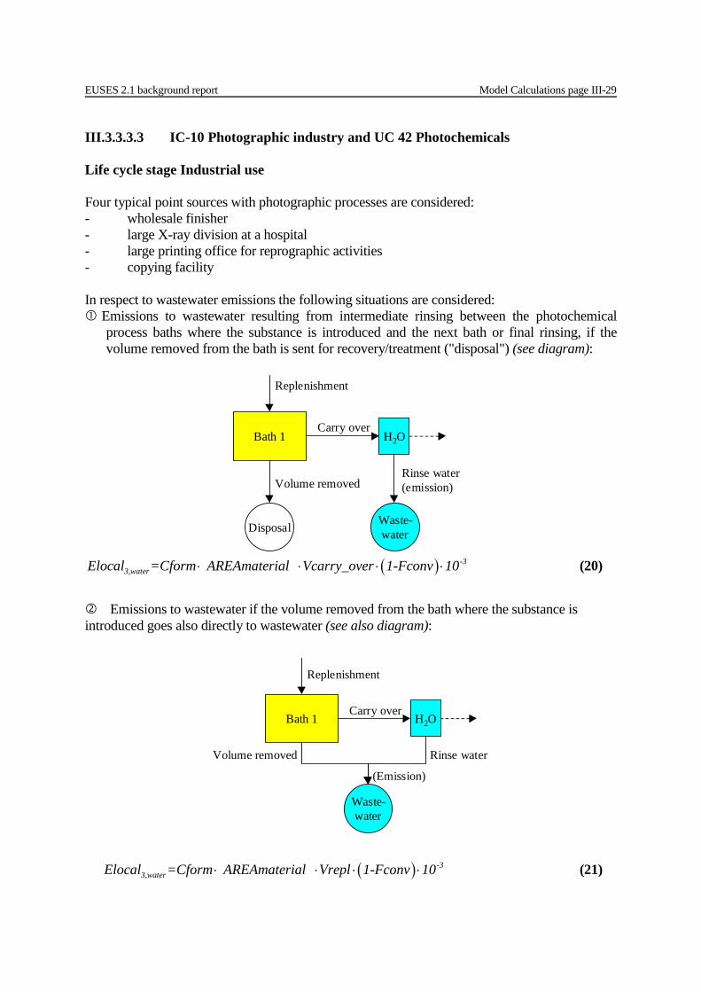
III.3.3.3.3 IC-10 Photographic industry and UC 42 Photochemicals Life cycle stage Industrial use Four typical point sources with photographic processes are considered: - wholesale finisher - large X-ray division at a hospital - large printing office for reprographic activities - copying facility In respect to wastewater emissions the following situations are considered: Emissions to wastewater resulting from intermediate rinsing between the photochemical
process baths where the substance is introduced and the next bath or final rinsing, if the volume removed from the bath is sent for recovery/treatment ("disposal") (see diagram):
Bath 1
Replenishment
Carry over
Disposal
Volume removed
H2O
Waste-water
Rinse water(emission)
( ) -3
3,waterElocal =Cform AREAmaterial Vcarry_over 1-Fconv 10⋅ ⋅ ⋅ ⋅ (20)
Emissions to wastewater if the volume removed from the bath where the substance is introduced goes also directly to wastewater (see also diagram):
Bath 1
Replenishment
Carry over
Volume removed
H2O
Waste-water
Rinse water
(Emission)
( ) -33,waterElocal =Cform AREAmaterial Vrepl 1-Fconv 10⋅ ⋅ ⋅ ⋅ (21)
Model Calculations page III-30 EUSES 2.1 background report
Input Cform concentration of substance in working solution [kgc.m-3] S/P AREAmaterial surface of processed film or paper [m2.d-1] S/P Vrepl replenishment rate [l.m-2] S/P Vcarry-over carry-over rate [l.m-2] S/P Fconv fraction of the substance removed or converted during process [-] D Output Elocal3, water local emission to wastewater [kgc.d-1] O Table III-13 Defaults for emission calculations.
Parameter Symbol Unit Value
concentration of substance in working solution Cform [kgc.m-3] 1)
surface of processed film or paper AREAmaterial [m2.d-1] 2)
replenishment rate Vrepl [l.m-2] 2)
carry-over rate Vcarry-over [l.m-2] 2)
fraction of substance removed or converted during process Fconv [-] 0 1) see pick-list Table III-18 2) see pick-list Table III-17 Emissions to wastewater when the carry-over of a processing bath, where the substance was
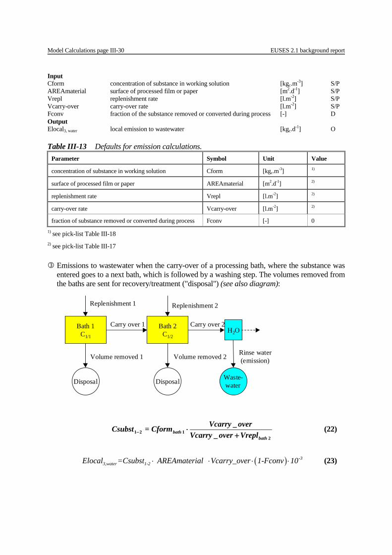
entered goes to a next bath, which is followed by a washing step. The volumes removed from the baths are sent for recovery/treatment ("disposal") (see also diagram):
2
121 __
bathbath VreploverVcarry
overVcarry Cform=Csubst+
⋅− (22)
( ) -33,water 1-2Elocal =Csubst AREAmaterial Vcarry_over 1-Fconv 10⋅ ⋅ ⋅ ⋅ (23)
Bath 1C1/1
Bath 2C1/2
Replenishment 1
Volume removed 1 Volume removed 2
Carry over 1 Carry over 2
Disposal Disposal
H2O
Waste-water
Replenishment 2
Rinse water(emission)
EUSES 2.1 background report Model Calculations page III-31
Input Csubst1-2 concentration of substance from first bath in the second bath [kgc.m-3] O Cformbath 1 concentration of substance in working solution of bath one [kgc.m-3] S/P AREAmaterial surface area of processed film or paper [m2.d-1] S/P Vreplbath 2 replenishment rate of second bath [l.m-2] S/P Vcarry-over carry-over rate [l.m-2] S/P Fconv fraction of the substance removed or converted during process [-] D Output Elocal3, water local emission to wastewater [kgc.d-1] O Table III-14 Defaults for emission calculations.
Parameter Symbol Unit Value
concentration of substance in first bath Cformbath 1 [kgc.m-3] 1)
surface of processed film or paper AREAmaterial [m2.d-1] 2)
replenishment rate Vrepl [l.m-2] 2)
carry-over rate Vcarry-over [l.m-2] 2)
fraction of substance removed or converted during process Fconv [-] 0 1) see pick-list Table III-18 2) see pick-list Table III-17
Release of substances from processing photographic materials:
( )Fconv−⋅⋅⋅ 1Fdiss alAREAmateriQsubst=Elocal water,3 (24)
Input Qsubst quantity of substance in the photographic material [kgc.m-2] S/P AREAmaterial surface area of processed film or paper [m2.d-1] S/P Fdiss fraction substance dissolved during processing [-] D Fconv fraction removed or converted during processing [-] D Output Elocal3, water local emission to wastewater [kgc.d-1] O Table III-15 Defaults for emission calculations.
Parameter Symbol Unit Value
Quantity of substance in the photographic material Qsubst [kgc.m-2] 1)
Surface area of processed film or paper AREAmaterial [m2] 2)
fraction of substance removed or converted during process Fconv [-] 0
fraction which dissolves during processing Fdiss [-] 1 1) see pick-list Table III-20 2) see pick-list Table III-17
Life cycle stage Waste treatment Release at the disposal company: ( ) ( )FredFconv −⋅−⋅⋅ 11 Vtreat Cform=Elocal water,6 (25)
Model Calculations page III-32 EUSES 2.1 background report
Input Cform concentration of substance in the fresh working solution [kgc.m-3] P Vtreat treated volume of working solution [m3.d-1] P Fconv fraction of the substance removed or converted during process [-] D Fred fraction of waste reduction [-] D Output Elocal6, water local emission to wastewater [kgc.d-1] O Table III-16 Defaults for emission calculations.
Parameter Symbol Unit Value
concentration of substance in working solution Cform [kgc.m-3] 1)
treated volume of working solution Vtreat [m3] 2)
fraction of substance removed or converted during process Fconv [-] 0
fraction of waste reduction Fred [-] 0 1) see pick-list Table III-18 2) see pick-list Table III-19
Table III-17 Pick-list for release estimation parameters replenish rate, Vrepl (l.m-²), carry-over rate, Vcarry-over (l.m-²) and treated area of photographic material, AREAmaterial (m².d-1). When there is no intermediate washing step the replenish rate is set to the lowest value. At direct introduction into wastewater the replenish rate is set to the highest value as worst case. Processa Bath Vreplb Vcarry-over AREAmaterial
wholesale finisher C-41 colour negative
developing 0.30–0.60 (0.45) 0.080 / 0.170c 680 bleaching 0.10–0.90 (0.50) fixing 0.40–0.90 (0.65) stabilising 0.90 (0.90)
RA-4 colour paper developing 0.06–0.12 (0.09) 0.040 / 0.070c 4950
bleach fixing 0.07–0.14 (0.10) RA-4 devided bleaching and fixing
developing 0.06–0.12 (0.09) 0.050 stopping 0.15–0.20 (0.175) bleaching 0.05–0.10 (0.075) fixing 0.055–0.100 (0.075) stabilising
E-6 colour reversal film
primary developing 0.9–1.8 (1.35) 0.080 / 0.170c 120 reversing 1.0–1.1 (1.05) colour developing 1.0–2.0 (1.5) conditioning 0.9–1.1 (1.0) bleaching 0.2 (0.2) fixing 0.4–1.0 (1.2) stabilising 1.0 9(1.0)
R-3 colour reversal paper
primary developing 0.17–0.33 (0.25) 0.050 350 colour developing 0.05–0.50 (0.275) bleach fixing 0.07–0.20 (0.135) stabilising
R-3 devided primary developing 0.17–0.33 (0.25)
EUSES 2.1 background report Model Calculations page III-33
Processa Bath Vreplb Vcarry-over AREAmaterial bleaching and fixing
colour developing 0.05-0.50 (0.275) bleaching 0.07–0.14 (0.105) fixing 0.055-0.100 (0.775) stabilising
BW-N developing 0.5-0.6 (0.55) 0.180 40 fixing 0.4-0.9 (0.65) BW-P developing 0.2-0.3 (0.25) 0.070 270 fixing 0.055-0.30 (0.178)
x-ray division BW-X med. developing 0.35-0.40 (0.375) 0.040 110
fixing 0.4-0.6 (0.50) BW-X tech. developing 0.5-0.6 (0.55) 0.040
fixing 0.8-1.2 (0.10) printing office
BW-R film developing 0.2-0.3 (0.25) 0.040 80
fixing 0.15-0.30 (0.225) copy facility
ECN-2 cine- and television- film negative
primary bath 0.375 0.180 35 colour developing
0.845
stopping 0.560 bleach accelerating 0.180 bleaching 0.180 fixing 0.560 stabilising 0.375
ECP-2 cine- and television positive
primary bath 0.374 0.180 350 colour developing 0.646 stopping 0.721 primary fixing 0.187 bleach accelerating 0.187 bleaching 0.187 secondary fixing 0.187 stabilising 0.374
VNF-1 cine- and television- film reversal
primary developing 0.348 0.180 35 primary stopping 2.254 colour developing 1.639 secondary stopping 1.332 bleach accelerating 0.410 bleaching 0.410 fixing 1.281 stabilising 0.615
a values of C-41, RA-4, E6, R-3, BW-P and BW-N are related to point source (a) -wholesale finisher values of BW-X are related to point source (b) –hospital values of BW-R are related to point source (c) -printing office values of ECN-2, ECP-2 and VNF-1 are related to point source (d) –copying facility b recycling processes of bath-solutions for point source (a) –wholesale finisher- are considered c carry-over rates for professional labs are different from wholesale finishers
Model Calculations page III-34 EUSES 2.1 background report Table III-18 Pick-list for the content of substance in processing solutions for every specific function, Cform (kgc.m-3), and the corresponding equation
(Eq = equation, Dev = developer, pH-reg = pH regulator, Antiox = antioxidant, Antifog = antifogging agent, Bleach = bleaching agent, Rehalog = rehalogenating agent, Fix = fixing agent, Stab = stabiliser, Seq = sequestering agent, Rev = reversing agent, Hard = hardening agent, Solv = auxiliary solvent, and Bl Acc = bleaching accelerator
Process Process bath Eq Dev pH-reg Antiox Antifog Bleach Rehalog Fix Stab Seq Rev Hard Solv Bl Acc UC 42 40 49 42 8 42 21 49 11 42 55/0 48 43 Wholesale finisher C-41 Developing 3 (n=2) 8 50 6 2 4 19 Bleaching 1 20 120 120 0.4 Fixing 1 20 8 150 Stabilising 2 2 RA-4 Developing 1 8 40 8 1.6 4 19 Stopping 1 Bleaching 1 10 50 52.5 0.4 Fixing 1 10 90 3 E-6 Primary developing 1 30 35 6.5 2 4 19 Reversing 3 (n=2) 2 Colour developing 1 10 50 6 1.6 4 19 Conditioning 2 20 Bleaching 3 (n=2) 150 80 0.4 Fixing 1 8 180 Stabilising 2 2 R-3 Primary developing 1 20 30 2 1.6 4 4 19 Colour developing 1 7 30 6.5 1.6 4 4 19 Bleach fixing 1 20 10 60 100 Stabilising 1 2 BW-N Developing 1 15 70 20 10 10 Fixing 1 20 20 150 5 BW-P Developing 1 15 70 20 10 10 Fixing 1 20 20 150 5 Printing office BW-R Developing 1 25 20 8 17 10 Fixing 1 15 15 120
EUSES 2.1 background report Model Calculations page III-35 Process Process bath Eq Dev PH-reg Antiox Antifog Bleach Rehalog Fix Stab Seq Rev Hard Solv Bl Acc UC 42 40 49 42 8 42 21 49 11 42 55/0 48 43 X-ray division BW-X Developing 1 20 60 20 17 10 Fixing 1 20 20 150 Copying facility ECN-2 Primary bath 3 (n=3) 0.8 55.6 Colour developing 3 (n=2) 3 13.5 1.4 0.43 4 19 Stopping 1 26.3 Bleach accelerating 1 15.8 6.3 0.4 Bleaching 1 8.5 30.4 80 120 Secondary fixing 1 12.9 68.2 Stabilising 1 8 ECP-2 Primary bath 3 (n=3) 0.8 55.6 Colour developing 3 (n=2) 11.5 9.5 2.4 0.8 4 19 Stopping 1 26.3 Primary fixing 1 8.9 0.4 54.8 Bleach accelerating 1 3.7 2.9 0.4 Bleaching 1 13.7 120 Secondary fixing 1 8.9 0.4 54.8 Stabilising 1 1.95 VNF-1 Primary developing 1 0.2 16.1 1.6 0.004 0.8 0.1 4 19 Primary stopping 1 16.7 Colour developing 1 6.7 2.6 4.3 0.02 0.06 4 19 Secondary stopping 1 16.7 Bleach accelerating 3 (n=3) 4.4 5.6 0.4 Bleaching 3 (n=2) 47.2 120 Fixing 1 5.2 93.9 Stabilising 1 2 N.B. ◘ If a specific bath is not mentioned the worst case default value for the substance with the specified function is used ◘ If the specific process for the photographic point source is not mentioned the worst case situation is used ◘ If the specific point source is not mentioned the worst case situation is used
Model Calculations page III-36 EUSES 2.1 background report
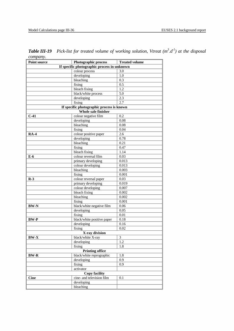
Table III-19 Pick-list for treated volume of working solution, Vtreat (m3.d-1) at the disposal company. Point source Photographic process Treated volume
If specific photographic process in unknown colour process 3.0 developing 1.0 bleaching 0.3 fixing 0.5 bleach fixing 1.2 black/white process 5.0 developing 2.3 fixing 2.7
If specific photographic process is known Whole sale finisher
C-41 colour negative film 0.2 developing 0.08 bleaching 0.08 fixing 0.04 RA-4 colour positive paper 2.6 developing 0.78 bleaching 0.21 fixing 0.47 bleach fixing 1.14 E-6 colour reversal film 0.03 primary developing 0.013 colour developing 0.013 bleaching 0.003 fixing 0.001 R-3 colour reversal paper 0.03 primary developing 0.019 colour developing 0.007 bleach fixing 0.002 bleaching 0.002 fixing 0.001 BW-N black/white negative film 0.06 developing 0.05 fixing 0.01 BW-P black/white positive paper 0.18 developing 0.16 fixing 0.02
X-ray division BW-X black/white X-ray 3 developing 1.2 fixing 1.8
Printing office BW-R black/white reprographic 1.8 developing 0.9 fixing 0.9 activator
Copy facility Cine cine- and television film 0.1 developing bleaching
EUSES 2.1 background report Model Calculations page III-37
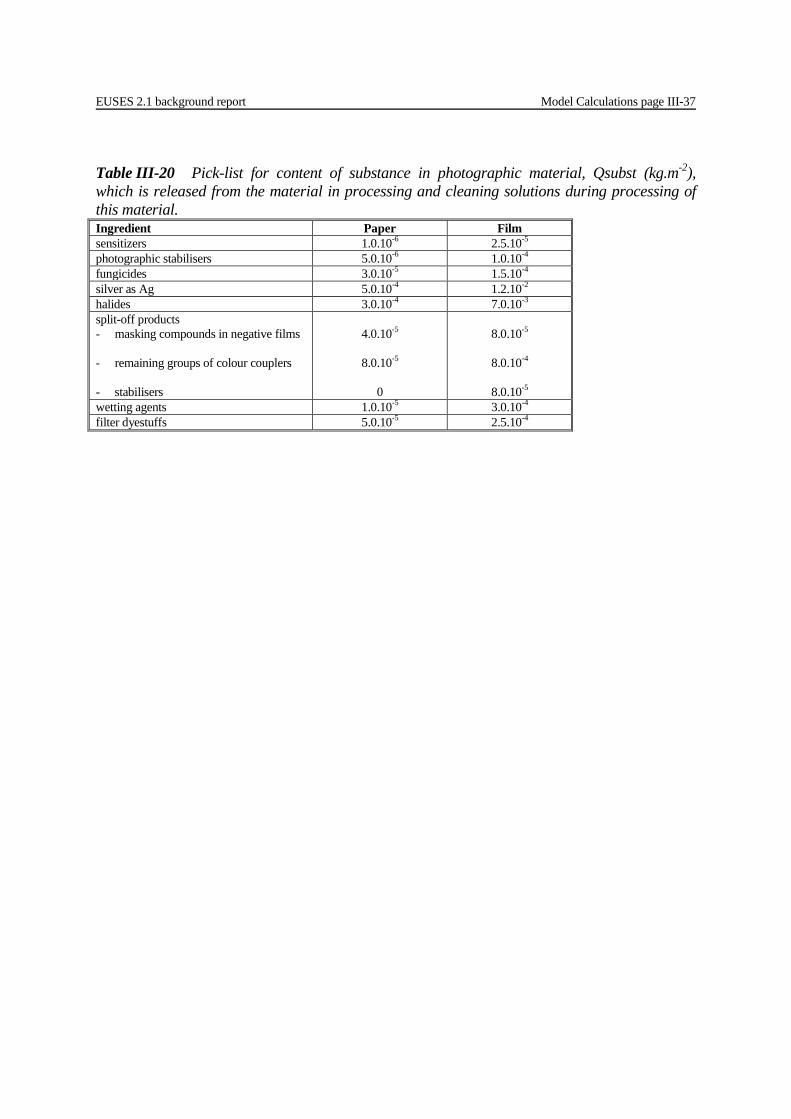
Table III-20 Pick-list for content of substance in photographic material, Qsubst (kg.m-2), which is released from the material in processing and cleaning solutions during processing of this material. Ingredient Paper Film sensitizers 1.0.10-6 2.5.10-5 photographic stabilisers 5.0.10-6 1.0.10-4 fungicides 3.0.10-5 1.5.10-4 silver as Ag 5.0.10-4 1.2.10-2 halides 3.0.10-4 7.0.10-3 split-off products - masking compounds in negative films - remaining groups of colour couplers - stabilisers
4.0.10-5
8.0.10-5
0
8.0.10-5
8.0.10-4
8.0.10-5
wetting agents 1.0.10-5 3.0.10-4 filter dyestuffs 5.0.10-5 2.5.10-4
Model Calculations page III-38 EUSES 2.1 background report
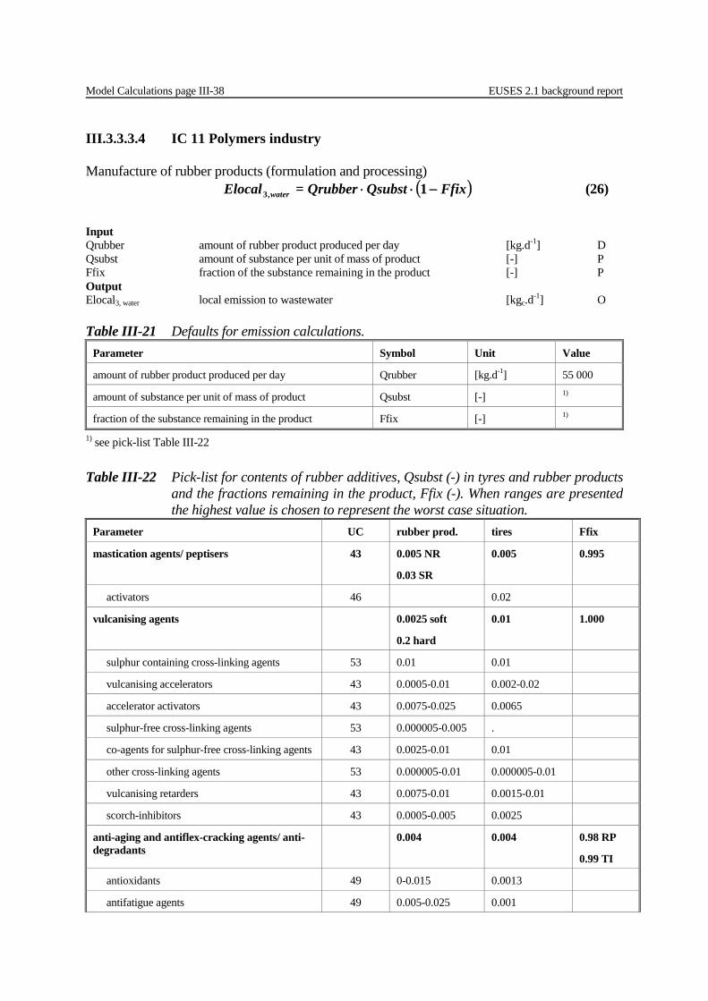
III.3.3.3.4 IC 11 Polymers industry Manufacture of rubber products (formulation and processing) ( )FfixQsubstQrubber=Elocal water −⋅⋅ 1,3 (26)
Input Qrubber amount of rubber product produced per day [kg.d-1] D Qsubst amount of substance per unit of mass of product [-] P Ffix fraction of the substance remaining in the product [-] P Output Elocal3, water local emission to wastewater [kgc.d-1] O Table III-21 Defaults for emission calculations.
Parameter Symbol Unit Value
amount of rubber product produced per day Qrubber [kg.d-1] 55 000
amount of substance per unit of mass of product Qsubst [-] 1)
fraction of the substance remaining in the product Ffix [-] 1)
1) see pick-list Table III-22 Table III-22 Pick-list for contents of rubber additives, Qsubst (-) in tyres and rubber products
and the fractions remaining in the product, Ffix (-). When ranges are presented the highest value is chosen to represent the worst case situation.
Parameter UC rubber prod. tires Ffix
mastication agents/ peptisers 43 0.005 NR
0.03 SR
0.005 0.995
activators 46 0.02
vulcanising agents 0.0025 soft
0.2 hard
0.01 1.000
sulphur containing cross-linking agents 53 0.01 0.01
vulcanising accelerators 43 0.0005-0.01 0.002-0.02
accelerator activators 43 0.0075-0.025 0.0065
sulphur-free cross-linking agents 53 0.000005-0.005 .
co-agents for sulphur-free cross-linking agents 43 0.0025-0.01 0.01
other cross-linking agents 53 0.000005-0.01 0.000005-0.01
vulcanising retarders 43 0.0075-0.01 0.0015-0.01
scorch-inhibitors 43 0.0005-0.005 0.0025
anti-aging and antiflex-cracking agents/ anti-degradants
0.004 0.004 0.98 RP
0.99 TI
antioxidants 49 0-0.015 0.0013
antifatigue agents 49 0.005-0.025 0.001
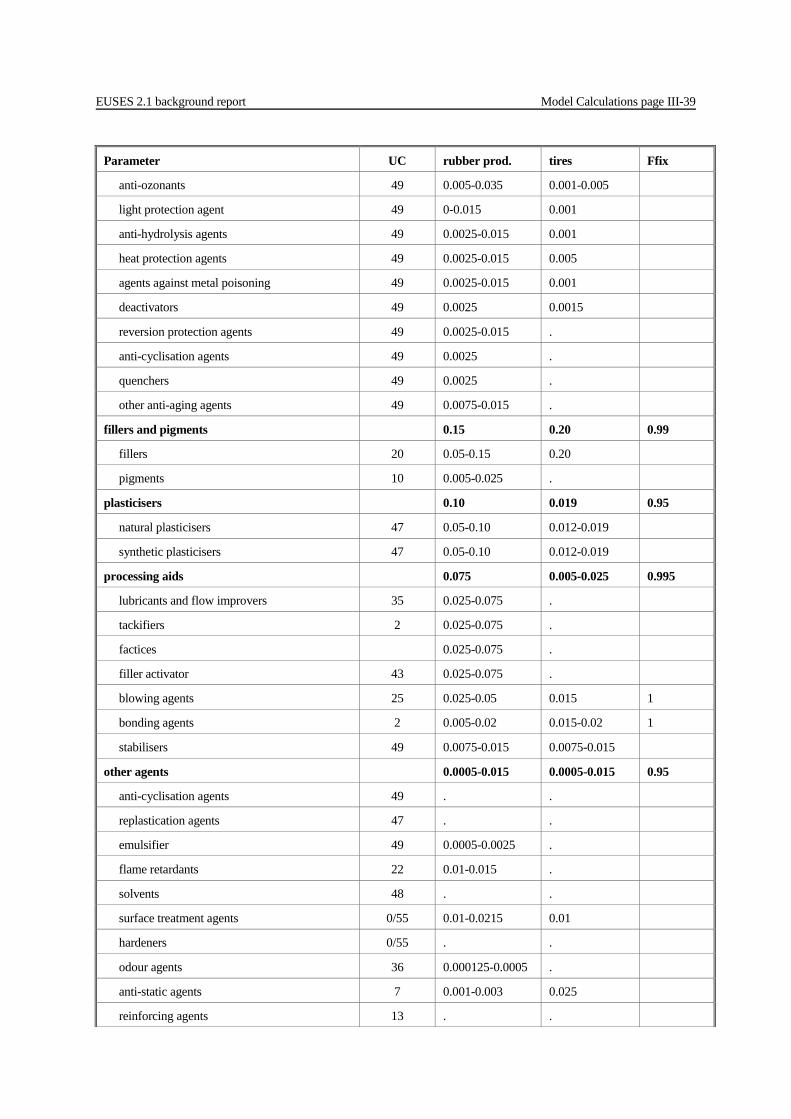
EUSES 2.1 background report Model Calculations page III-39
Parameter UC rubber prod. tires Ffix
anti-ozonants 49 0.005-0.035 0.001-0.005
light protection agent 49 0-0.015 0.001
anti-hydrolysis agents 49 0.0025-0.015 0.001
heat protection agents 49 0.0025-0.015 0.005
agents against metal poisoning 49 0.0025-0.015 0.001
deactivators 49 0.0025 0.0015
reversion protection agents 49 0.0025-0.015 .
anti-cyclisation agents 49 0.0025 .
quenchers 49 0.0025 .
other anti-aging agents 49 0.0075-0.015 .
fillers and pigments 0.15 0.20 0.99
fillers 20 0.05-0.15 0.20
pigments 10 0.005-0.025 .
plasticisers 0.10 0.019 0.95
natural plasticisers 47 0.05-0.10 0.012-0.019
synthetic plasticisers 47 0.05-0.10 0.012-0.019
processing aids 0.075 0.005-0.025 0.995
lubricants and flow improvers 35 0.025-0.075 .
tackifiers 2 0.025-0.075 .
factices 0.025-0.075 .
filler activator 43 0.025-0.075 .
blowing agents 25 0.025-0.05 0.015 1
bonding agents 2 0.005-0.02 0.015-0.02 1
stabilisers 49 0.0075-0.015 0.0075-0.015
other agents 0.0005-0.015 0.0005-0.015 0.95
anti-cyclisation agents 49 . .
replastication agents 47 . .
emulsifier 49 0.0005-0.0025 .
flame retardants 22 0.01-0.015 .
solvents 48 . .
surface treatment agents 0/55 0.01-0.0215 0.01
hardeners 0/55 . .
odour agents 36 0.000125-0.0005 .
anti-static agents 7 0.001-0.003 0.025
reinforcing agents 13 . .
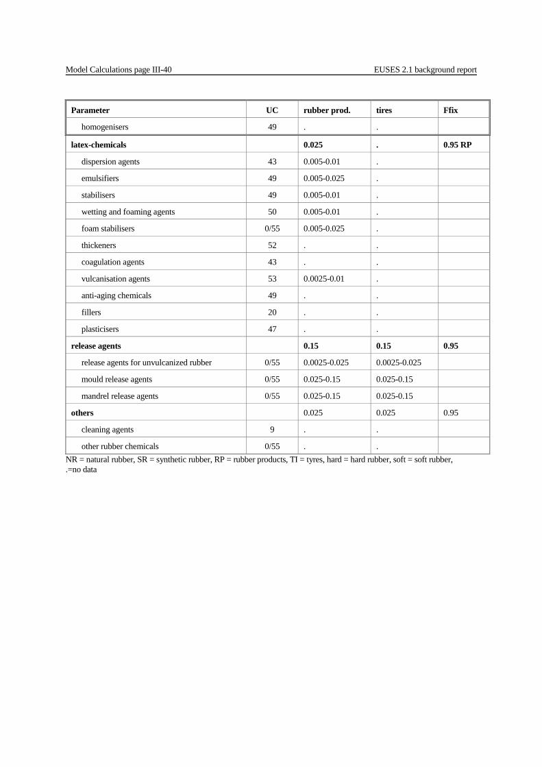
Model Calculations page III-40 EUSES 2.1 background report
Parameter UC rubber prod. tires Ffix
homogenisers 49 . .
latex-chemicals 0.025 . 0.95 RP
dispersion agents 43 0.005-0.01 .
emulsifiers 49 0.005-0.025 .
stabilisers 49 0.005-0.01 .
wetting and foaming agents 50 0.005-0.01 .
foam stabilisers 0/55 0.005-0.025 .
thickeners 52 . .
coagulation agents 43 . .
vulcanisation agents 53 0.0025-0.01 .
anti-aging chemicals 49 . .
fillers 20 . .
plasticisers 47 . .
release agents 0.15 0.15 0.95
release agents for unvulcanized rubber 0/55 0.0025-0.025 0.0025-0.025
mould release agents 0/55 0.025-0.15 0.025-0.15
mandrel release agents 0/55 0.025-0.15 0.025-0.15
others 0.025 0.025 0.95
cleaning agents 9 . .
other rubber chemicals 0/55 . . NR = natural rubber, SR = synthetic rubber, RP = rubber products, TI = tyres, hard = hard rubber, soft = soft rubber, .=no data

EUSES 2.1 background report Model Calculations page III-41
III.3.3.3.5 IC 12 Pulp, paper and board industry Emissions to surface water of chemicals used in the manufacture of paper (including coating of paper) and recycling of paper. Life cycle stage Industrial use, Paper production applied amount per ton of paper: ( ) ( )FclosureFfix −⋅−⋅⋅ 11 Qpaper Qsubst=Elocal water,3 (27)
Input Qsubst consumption of substance per tonne of paper [kgc.tonne-1] S/P Qpaper quantity of paper produced on one site per day [tonnes.d-1] P Ffix degree of fixation [-] S/P Fclosure degree of closure of the water system [-] P Output Elocal3, water local emission to wastewater [kgc.d-1] O Table III-23 Defaults for emission calculations
Parameter Symbol Unit Value
consumption of substance per tonne of paper Qsubst [kgc.tonne-1] 1)
quantity of paper produced on one site per day Qpaper [tonne.d-1] 2)
degree of fixation Ffix [-] 3)
degree of closure of the water system Fclosure [-] 2)
1) see pick-lists Table III-26 and Table III-27 2) see pick-list Table III-25 3) see pick-lists Table III-26 and Table III-28
Estimation if concentration of the substance in process water is used: ( )Ffix−⋅⋅⋅ 1 QpaperQwater Csubst=Elocal water,3 (28)
Input Csubst concentration of substance in process water [kgc.m-3] S/P Qwater quantity of water used per tonne of paper [m3.tonne-1] P Qpaper quantity of paper produced on one site per day [tonne.d-1] P Ffix degree of fixation [-] S/P Output Elocal3,water local emission to wastewater [kgc.d-1] O
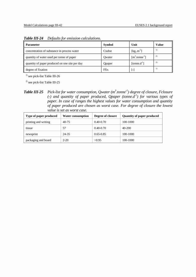
Model Calculations page III-42 EUSES 2.1 background report
Table III-24 Defaults for emission calculations. Parameter Symbol Unit Value
concentration of substance in process water Csubst [kgc.m-3] 1)
quantity of water used per tonne of paper Qwater [m3.tonne-1] 2)
quantity of paper produced on one site per day Qpaper [tonne.d-1] 2)
degree of fixation Ffix [-] 1) 1) see pick-list Table III-26 2) see pick-list Table III-25
Table III-25 Pick-list for water consumption, Qwater (m3.tonne-1) degree of closure, Fclosure
(-) and quantity of paper produced, Qpaper (tonne.d-1) for various types of paper. In case of ranges the highest values for water consumption and quantity of paper produced are chosen as worst case. For degree of closure the lowest value is set as worst case.
Type of paper produced Water consumption Degree of closure Quantity of paper produced
printing and writing 40-75 0.40-0.70 100-1000
tissue 57 0.40-0.70 40-200
newsprint 24-35 0.65-0.85 100-1000
packaging and board 2-20 >0.95 100-1000
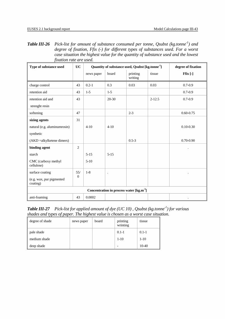
EUSES 2.1 background report Model Calculations page III-43
Table III-26 Pick-list for amount of substance consumed per tonne, Qsubst (kg.tonne-1) and degree of fixation, Ffix (-) for different types of substances used. For a worst case situation the highest value for the quantity of substance used and the lowest fixation rate are used.
Type of substance used UC Quantity of substance used, Qsubst [kg.tonne-1] degree of fixation
news paper board printing writing
tissue Ffix [-]
charge control 43 0.2-1 0.3 0.03 0.03 0.7-0.9
retention aid 43 1-5 1-5 0.7-0.9
retention aid and
strenght resin
43 20-30 2-12.5 0.7-0.9
softening 47 2-3 0.60-0.75
sizing agents
natural (e.g. aluminumrosin)
synthetic
(AKD =alkylketene dimers)
31
4-10
4-10
0.5-3
0.10-0.30
0.70-0.90
binding agent
starch
CMC (carboxy methyl cellulose)
2
5-15
5-10
5-15
.
surface coating
(e.g. wax, pur pigmented coating)
55/0
1-8 . .
Concentration in process water [kg.m-3]
anti-foaming 43 0.0002 .
Table III-27 Pick-list for applied amount of dye (UC 10) , Qsubst (kg.tonne-1) for various shades and types of paper. The highest value is chosen as a worst case situation.
degree of shade news paper board printing wrinting
tissue
pale shade
medium shade
deep shade
0.1-1
1-10
-
0.1-1
1-10
10-40
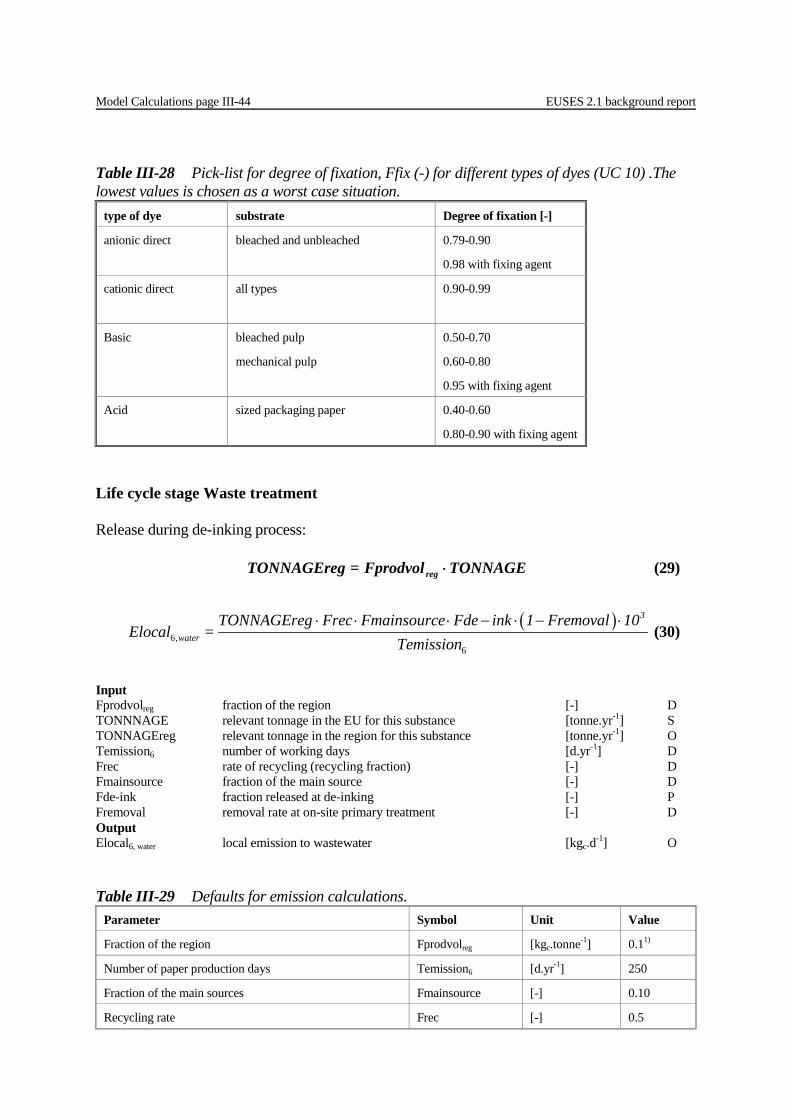
Model Calculations page III-44 EUSES 2.1 background report
Table III-28 Pick-list for degree of fixation, Ffix (-) for different types of dyes (UC 10) .The lowest values is chosen as a worst case situation.
type of dye substrate Degree of fixation [-]
anionic direct bleached and unbleached 0.79-0.90
0.98 with fixing agent
cationic direct all types 0.90-0.99
Basic bleached pulp
mechanical pulp
0.50-0.70
0.60-0.80
0.95 with fixing agent
Acid sized packaging paper 0.40-0.60
0.80-0.90 with fixing agent
Life cycle stage Waste treatment Release during de-inking process: TONNAGEFprodvol=TONNAGEreg reg ⋅ (29)
( )6,
6
3
water
TONNAGEreg Frec Fmainsource Fde ink 1 Fremoval 10Elocal =
Temission⋅ ⋅ ⋅ − ⋅ − ⋅
(30)
Input Fprodvolreg fraction of the region [-] D TONNNAGE relevant tonnage in the EU for this substance [tonne.yr-1] S TONNAGEreg relevant tonnage in the region for this substance [tonne.yr-1] O Temission6 number of working days [d.yr-1] D Frec rate of recycling (recycling fraction) [-] D Fmainsource fraction of the main source [-] D Fde-ink fraction released at de-inking [-] P Fremoval removal rate at on-site primary treatment [-] D Output Elocal6, water local emission to wastewater [kgc.d-1] O Table III-29 Defaults for emission calculations.
Parameter Symbol Unit Value
Fraction of the region Fprodvolreg [kgc.tonne-1] 0.11)
Number of paper production days Temission6 [d.yr-1] 250
Fraction of the main sources Fmainsource [-] 0.10
Recycling rate Frec [-] 0.5

EUSES 2.1 background report Model Calculations page III-45
fraction released at de-inking Fde-ink [-] 2)
removal rate at on-site primary treatment
- easily soluble (> 1000 mg.l-1)
- insoluble (≤ 1000 mg.l-1)
Fremoval [-]
0.2
0.9 1) for new substances or existing substances produced at low volumes and which are not used homogeneously throughout the EU, it can be assumed in a first approach that Fprodvolreg = 1 2) see pick-list Table III-30 or Table III-31 Table III-30 Fraction of ink released at de-inking process, Fde-ink (-) for various types of ink.
Highest fraction of de-inking is used as a worst case value. Type of ink Fde-ink [-]
mineral oil based 0.14-0.28
flexographic 0.30-0.90
non-impact toners 0.06-0.28
Table III-31 Fraction of ink released at de-inking process, Fde-ink (-) for various ink drying
processes. Highest fraction released at de-inking is used as a worst case value. method of ink drying Fde-ink [-]
absorption, penetration, evaporation 0-0.20
oxidation or IR radiation 0.05-0.40
hot polymerisation or UV-fixation 0.10-0.60
ink-jet, laser or xerographic copying 0.40-0.70
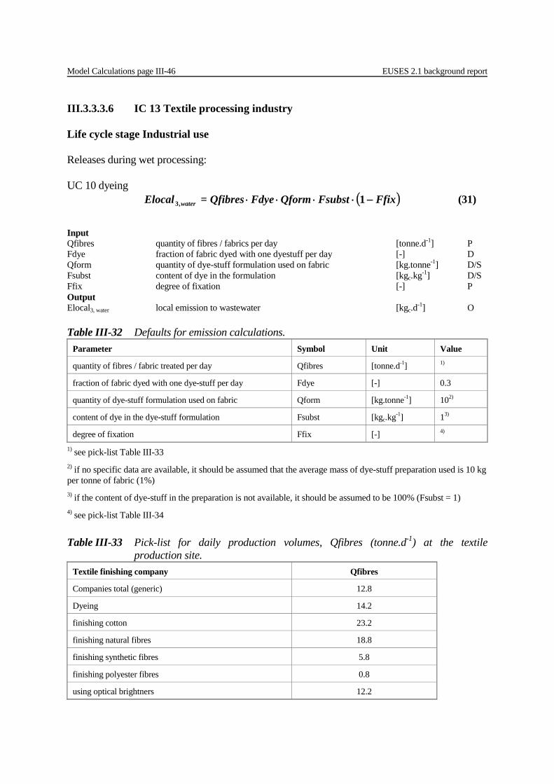
Model Calculations page III-46 EUSES 2.1 background report
III.3.3.3.6 IC 13 Textile processing industry Life cycle stage Industrial use Releases during wet processing: UC 10 dyeing ( )FfixFsubstQformFdye Qfibres=Elocal water −⋅⋅⋅⋅ 1,3 (31)
Input Qfibres quantity of fibres / fabrics per day [tonne.d-1] P Fdye fraction of fabric dyed with one dyestuff per day [-] D Qform quantity of dye-stuff formulation used on fabric [kg.tonne-1] D/S Fsubst content of dye in the formulation [kgc.kg-1] D/S Ffix degree of fixation [-] P Output Elocal3, water local emission to wastewater [kgc.d-1] O Table III-32 Defaults for emission calculations.
Parameter Symbol Unit Value
quantity of fibres / fabric treated per day Qfibres [tonne.d-1] 1)
fraction of fabric dyed with one dye-stuff per day Fdye [-] 0.3
quantity of dye-stuff formulation used on fabric Qform [kg.tonne-1] 102)
content of dye in the dye-stuff formulation Fsubst [kgc.kg-1] 13)
degree of fixation Ffix [-] 4) 1) see pick-list Table III-33 2) if no specific data are available, it should be assumed that the average mass of dye-stuff preparation used is 10 kg per tonne of fabric (1%) 3) if the content of dye-stuff in the preparation is not available, it should be assumed to be 100% (Fsubst = 1) 4) see pick-list Table III-34 Table III-33 Pick-list for daily production volumes, Qfibres (tonne.d-1) at the textile
production site. Textile finishing company Qfibres
Companies total (generic) 12.8
Dyeing 14.2
finishing cotton 23.2
finishing natural fibres 18.8
finishing synthetic fibres 5.8
finishing polyester fibres 0.8
using optical brightners 12.2
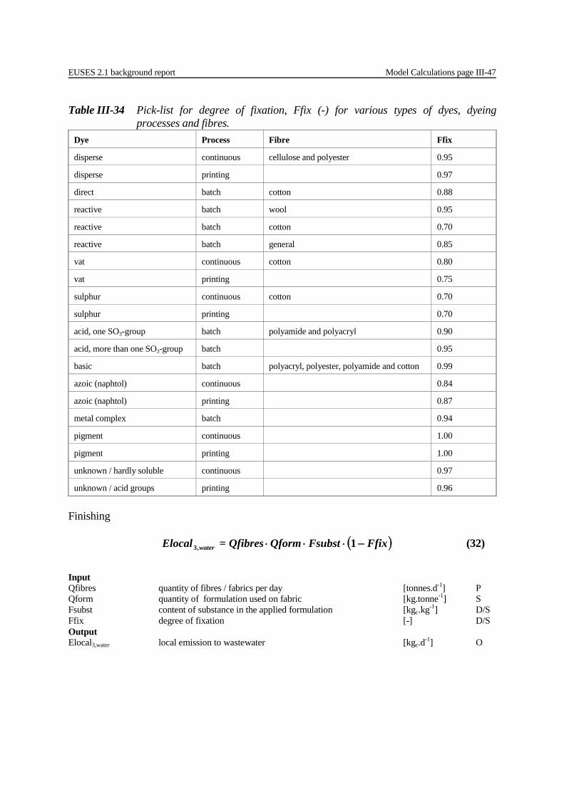
EUSES 2.1 background report Model Calculations page III-47
Table III-34 Pick-list for degree of fixation, Ffix (-) for various types of dyes, dyeing processes and fibres.
Dye Process Fibre Ffix
disperse continuous cellulose and polyester 0.95
disperse printing 0.97
direct batch cotton 0.88
reactive batch wool 0.95
reactive batch cotton 0.70
reactive batch general 0.85
vat continuous cotton 0.80
vat printing 0.75
sulphur continuous cotton 0.70
sulphur printing 0.70
acid, one SO3-group batch polyamide and polyacryl 0.90
acid, more than one SO3-group batch 0.95
basic batch polyacryl, polyester, polyamide and cotton 0.99
azoic (naphtol) continuous 0.84
azoic (naphtol) printing 0.87
metal complex batch 0.94
pigment continuous 1.00
pigment printing 1.00
unknown / hardly soluble continuous 0.97
unknown / acid groups printing 0.96
Finishing ( )FfixFsubstQformQfibres=Elocal water −⋅⋅⋅ 1,3 (32)
Input Qfibres quantity of fibres / fabrics per day [tonnes.d-1] P Qform quantity of formulation used on fabric [kg.tonne-1] S Fsubst content of substance in the applied formulation [kgc.kg-1] D/S Ffix degree of fixation [-] D/S Output Elocal3,water local emission to wastewater [kgc.d-1] O

Model Calculations page III-48 EUSES 2.1 background report
Table III-35 Defaults for emission calculations. Parameter Symbol Unit Value
quantity of fibres / fabric treated per day Qfibres [tonne.d-1] 1)
quantity of formulation used on fabric Qform [kg.tonne-1] -
content of substance in the applied formulation Fsubst [kgc.kg-1] 12)
degree of fixation Ffix [-] 0 1) see pick-list Table III-33 2) if the content of the substance in the preparation is not available, it should be assumed to be 100%
Life cycle stage Service life The release to wastewater (STP) is calculated as:
( )
1
5
1,5
3,5
,5,
110_−
=∑ −⋅⋅⋅⋅
yTservice
ywaterkwaterreg
waterk Temission
FtotQsubstFFprodvol=RELEASEreg
k
(33)
5, ,5,1
m
water k waterk
RELEASEreg = RELEASEreg=∑ (34)
5, 5 5,water waterElocal = Fmainsource RELEASEreg⋅ (35) Input Qsubst_totk annual input of the substance in article k [tonnes.yr-1] S Fprodvolreg fraction of EU volume for region [-] D Tservicek service life of article k [yr] P F5,water fraction of the tonnage release over one year during the service [-] S to waste water Temission5 number of emission days per year [d.yr-1] D Fmainsource5 fraction of the main source (STP) [-] D RELEASEregk,5,water release to waste water for article k [kgc.d-1] O RELEASEreg5,water release to waste water for all articles [kgc.d-1] O Output Elocal5, water local emission to wastewater [kgc.d-1] O
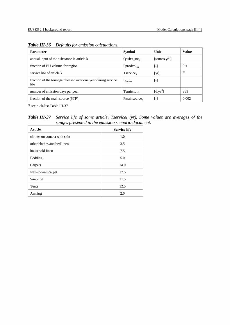
EUSES 2.1 background report Model Calculations page III-49
Table III-36 Defaults for emission calculations. Parameter Symbol Unit Value
annual input of the substance in article k Qsubst_totk [tonnes.yr-1]
fraction of EU volume for region Fprodvolreg [-] 0.1
service life of article k Tservicek [yr] 1)
fraction of the tonnage released over one year during service life
F5,water [-]
number of emission days per year Temission5 [d.yr-1] 365
fraction of the main source (STP) Fmainsource5 [-] 0.002 1) see pick-list Table III-37 Table III-37 Service life of some article, Tservicek (yr). Some values are averages of the
ranges presented in the emission scenario document. Article Service life
clothes on contact with skin 1.0
other clothes and bed linen 3.5
household linen 7.5
Bedding 5.0
Carpets 14.0
wall-to-wall carpet 17.5
Sunblind 11.5
Tents 12.5
Awning 2.0
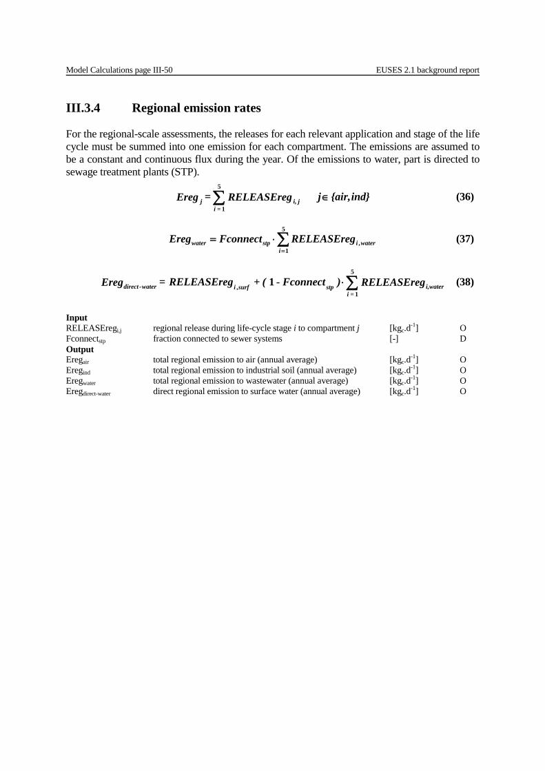
Model Calculations page III-50 EUSES 2.1 background report
III.3.4 Regional emission rates For the regional-scale assessments, the releases for each relevant application and stage of the life cycle must be summed into one emission for each compartment. The emissions are assumed to be a constant and continuous flux during the year. Of the emissions to water, part is directed to sewage treatment plants (STP).
Input RELEASEregi,j regional release during life-cycle stage i to compartment j [kgc.d-1] O Fconnectstp fraction connected to sewer systems [-] D Output Eregair total regional emission to air (annual average) [kgc.d-1] O Eregind total regional emission to industrial soil (annual average) [kgc.d-1] O Eregwater total regional emission to wastewater (annual average) [kgc.d-1] O Eregdirect-water direct regional emission to surface water (annual average) [kgc.d-1] O
ind}{air, j RELEASEreg = Ereg ji,= i
j ∈∑5
1
(36)
∑=
⋅=5
1,
iwateristpwater RELEASEregFconnectEreg (37)
RELEASEreg )Fconnect - ( + RELEASEreg= Ereg wateri,= i
stpsurf,iwater-direct ∑⋅5
1
1 (38)

EUSES 2.1 background report Model Calculations page III-51
III.3.5 Continental emission rates On the continental scale, all emissions for each compartment are summed over the relevant stages of the life cycle and the various applications, as was done for the regional scale.
Input RELEASEconti,j continental release during life-cycle stage i to compartment j [kgc.d-1] O Fconnectstp fraction connected to sewer systems [-] D Output Econtair continental emission to air (annual average) [kgc.d-1] O Econtind continental emission to industrial soil (annual average) [kgc.d-1] O Econtwater continental emission to wastewater (annual average) [kgc.d-1] O Econtdirect-water direct continental emission to surface water (annual average) [kgc.d-1] O
ind}{air, j tRELEASEcon = Econt ji,= i
j ∈∑5
1
(39)
tRELEASEcon Fconnect= Econt wateri,= i
stpwater ∑⋅5
1
(40)
water,i= i
stpsurf,iwaterdirecttRELEASEcon )Fconnect-( + tRELEASEcon= Econt ∑⋅−
5
1
1 (41)
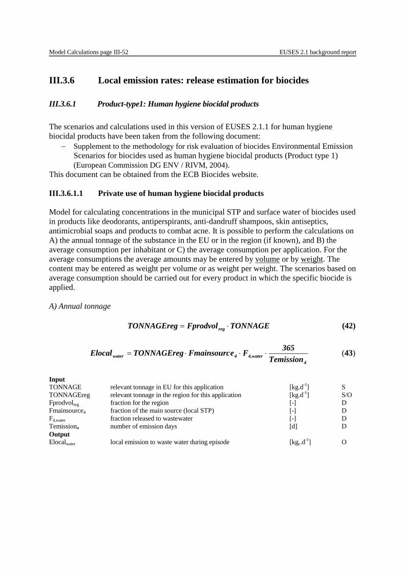
Model Calculations page III-52 EUSES 2.1 background report
III.3.6 Local emission rates: release estimation for biocides III.3.6.1 Product-type1: Human hygiene biocidal products The scenarios and calculations used in this version of EUSES 2.1.1 for human hygiene biocidal products have been taken from the following document:
− Supplement to the methodology for risk evaluation of biocides Environmental Emission Scenarios for biocides used as human hygiene biocidal products (Product type 1) (European Commission DG ENV / RIVM, 2004).
This document can be obtained from the ECB Biocides website. III.3.6.1.1 Private use of human hygiene biocidal products Model for calculating concentrations in the municipal STP and surface water of biocides used in products like deodorants, antiperspirants, anti-dandruff shampoos, skin antiseptics, antimicrobial soaps and products to combat acne. It is possible to perform the calculations on A) the annual tonnage of the substance in the EU or in the region (if known), and B) the average consumption per inhabitant or C) the average consumption per application. For the average consumptions the average amounts may be entered by volume or by weight. The content may be entered as weight per volume or as weight per weight. The scenarios based on average consumption should be carried out for every product in which the specific biocide is applied. A) Annual tonnage TONNAGEFprodvolTONNAGEreg reg ⋅= (42)
4
water4,4water Temission365FeFmainsourcTONNAGEregElocal ⋅⋅⋅= (43)
Input TONNAGE relevant tonnage in EU for this application [kg.d-1] S TONNAGEreg relevant tonnage in the region for this application [kg.d-1] S/O Fprodvolreg fraction for the region [-] D Fmainsource4 fraction of the main source (local STP) [-] D F4,water fraction released to wastewater [-] D Temission4 number of emission days [d] D Output Elocalwater local emission to waste water during episode [kgc.d-1] O
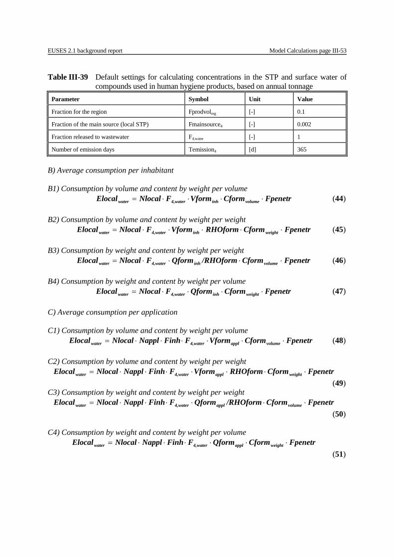
EUSES 2.1 background report Model Calculations page III-53
Table III-39 Default settings for calculating concentrations in the STP and surface water of compounds used in human hygiene products, based on annual tonnage
Parameter Symbol Unit Value
Fraction for the region Fprodvolreg [-] 0.1
Fraction of the main source (local STP) Fmainsource4 [-] 0.002
Fraction released to wastewater F4,water [-] 1
Number of emission days Temission4 [d] 365
B) Average consumption per inhabitant B1) Consumption by volume and content by weight per volume FpenetrCformVformFNlocalElocal volumeinhwater4,water ⋅⋅⋅⋅= (44) B2) Consumption by volume and content by weight per weight FpenetrCformRHOformVformFNlocalElocal weightinhwater4,water ⋅⋅⋅⋅⋅= (45) B3) Consumption by weight and content by weight per weight FpenetrCform/RHOformQformFNlocalElocal volumeinhwater4,water ⋅⋅⋅⋅= (46) B4) Consumption by weight and content by weight per volume FpenetrCformQformFNlocalElocal weightinhwater4,water ⋅⋅⋅⋅= (47) C) Average consumption per application C1) Consumption by volume and content by weight per volume FpenetrCformVformFFinhNapplNlocalElocal volumeapplwater4,water ⋅⋅⋅⋅⋅⋅= (48) C2) Consumption by volume and content by weight per weight FpenetrCformRHOformVformFFinhNapplNlocalElocal weightapplwater4,water ⋅⋅⋅⋅⋅⋅⋅= (49) C3) Consumption by weight and content by weight per weight FpenetrCform/RHOformQformFFinhNapplNlocalElocal volumeapplwater4,water ⋅⋅⋅⋅⋅⋅= (50) C4) Consumption by weight and content by weight per volume FpenetrCformQformFFinhNapplNlocalElocal weightapplwater4,water ⋅⋅⋅⋅⋅⋅= (51)
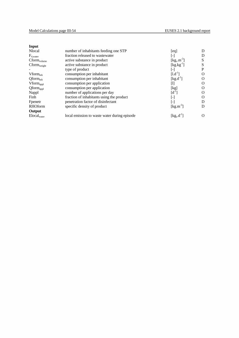
Model Calculations page III-54 EUSES 2.1 background report
Input Nlocal number of inhabitants feeding one STP [eq] D F4,water fraction released to wastewater [-] D Cformvolume active substance in product [kgc.m-3] S Cformweight active substance in product [kg.kg-1] S - type of product [-] P Vforminh consumption per inhabitant [l.d-1] O Qforminh consumption per inhabitant [kg.d-1] O Vformappl consumption per application [l] O Qformappl consumption per application [kg] O Nappl number of applications per day [d-1] O Finh fraction of inhabitants using the product [-] O Fpenetr penetration factor of disinfectant [-] D RHOform specific density of product [kg.m-3] D Output Elocalwater local emission to waste water during episode [kgc.d-1] O
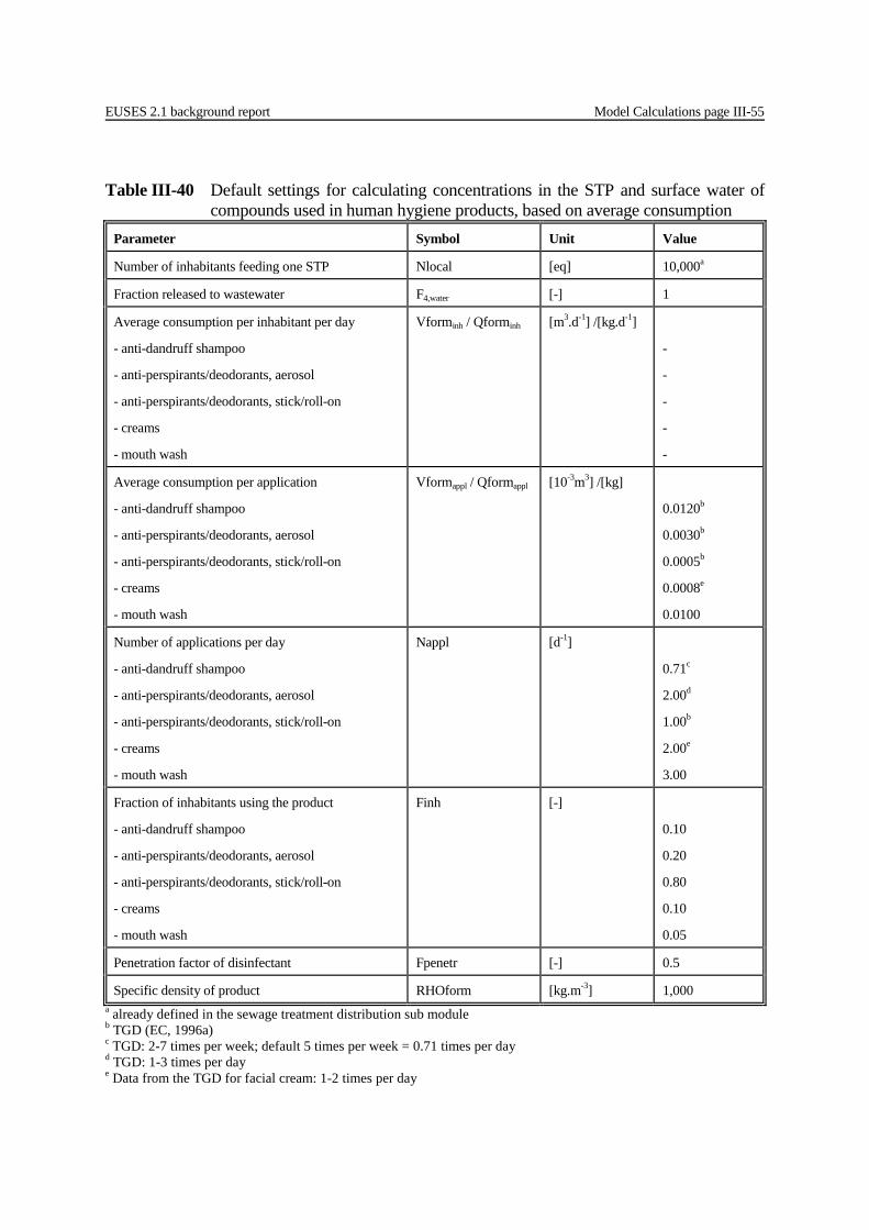
EUSES 2.1 background report Model Calculations page III-55
Table III-40 Default settings for calculating concentrations in the STP and surface water of
compounds used in human hygiene products, based on average consumption Parameter Symbol Unit Value
Number of inhabitants feeding one STP Nlocal [eq] 10,000a
Fraction released to wastewater F4,water [-] 1
Average consumption per inhabitant per day
- anti-dandruff shampoo
- anti-perspirants/deodorants, aerosol
- anti-perspirants/deodorants, stick/roll-on
- creams
- mouth wash
Vforminh / Qforminh [m3.d-1] /[kg.d-1]
-
-
-
-
-
Average consumption per application
- anti-dandruff shampoo
- anti-perspirants/deodorants, aerosol
- anti-perspirants/deodorants, stick/roll-on
- creams
- mouth wash
Vformappl / Qformappl [10-3m3] /[kg]
0.0120b
0.0030b
0.0005b
0.0008e
0.0100
Number of applications per day
- anti-dandruff shampoo
- anti-perspirants/deodorants, aerosol
- anti-perspirants/deodorants, stick/roll-on
- creams
- mouth wash
Nappl [d-1]
0.71c
2.00d
1.00b
2.00e
3.00
Fraction of inhabitants using the product
- anti-dandruff shampoo
- anti-perspirants/deodorants, aerosol
- anti-perspirants/deodorants, stick/roll-on
- creams
- mouth wash
Finh [-]
0.10
0.20
0.80
0.10
0.05
Penetration factor of disinfectant Fpenetr [-] 0.5
Specific density of product RHOform [kg.m-3] 1,000 a already defined in the sewage treatment distribution sub module b TGD (EC, 1996a) c TGD: 2-7 times per week; default 5 times per week = 0.71 times per day d TGD: 1-3 times per day e Data from the TGD for facial cream: 1-2 times per day
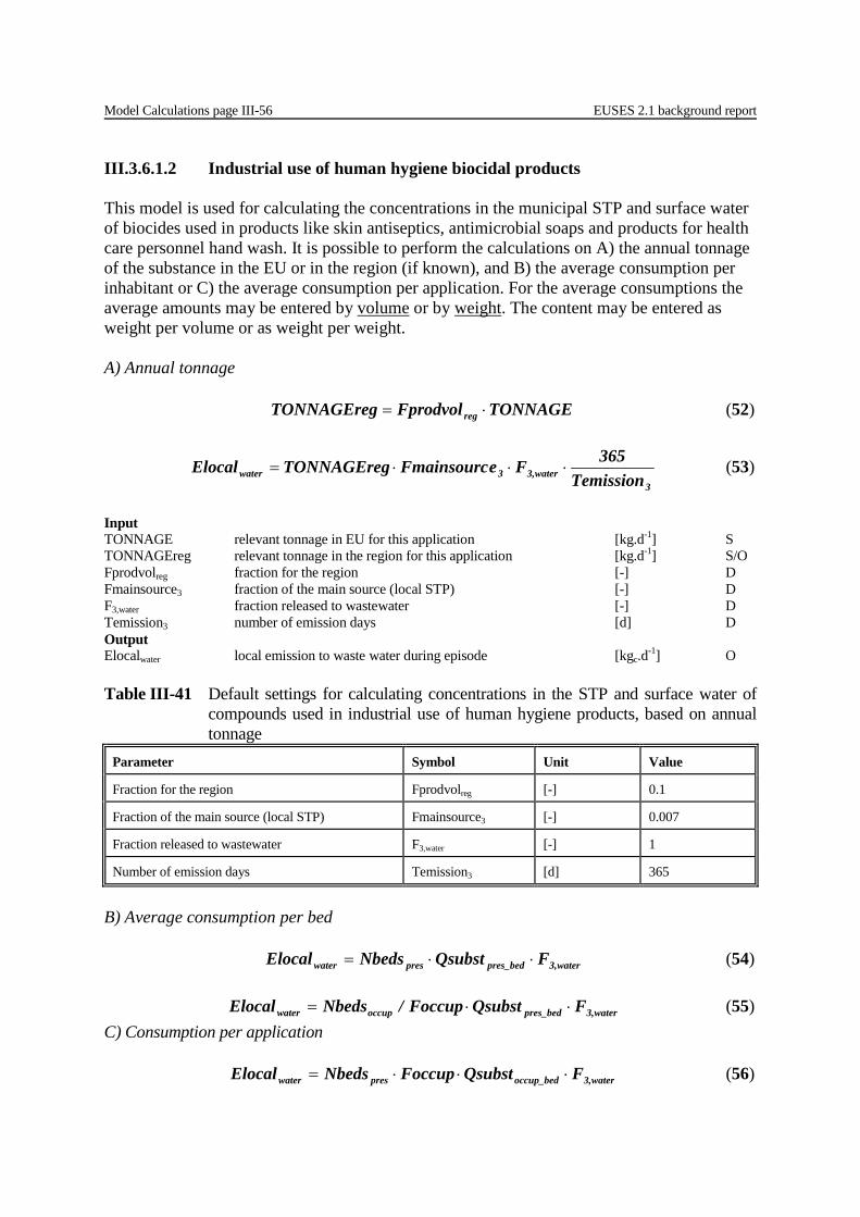
Model Calculations page III-56 EUSES 2.1 background report
III.3.6.1.2 Industrial use of human hygiene biocidal products This model is used for calculating the concentrations in the municipal STP and surface water of biocides used in products like skin antiseptics, antimicrobial soaps and products for health care personnel hand wash. It is possible to perform the calculations on A) the annual tonnage of the substance in the EU or in the region (if known), and B) the average consumption per inhabitant or C) the average consumption per application. For the average consumptions the average amounts may be entered by volume or by weight. The content may be entered as weight per volume or as weight per weight. A) Annual tonnage TONNAGEFprodvolTONNAGEreg reg ⋅= (52)
3
water3,3water Temission365FeFmainsourcTONNAGEregElocal ⋅⋅⋅= (53)
Input TONNAGE relevant tonnage in EU for this application [kg.d-1] S TONNAGEreg relevant tonnage in the region for this application [kg.d-1] S/O Fprodvolreg fraction for the region [-] D Fmainsource3 fraction of the main source (local STP) [-] D F3,water fraction released to wastewater [-] D Temission3 number of emission days [d] D Output Elocalwater local emission to waste water during episode [kgc.d-1] O Table III-41 Default settings for calculating concentrations in the STP and surface water of
compounds used in industrial use of human hygiene products, based on annual tonnage
Parameter Symbol Unit Value
Fraction for the region Fprodvolreg [-] 0.1
Fraction of the main source (local STP) Fmainsource3 [-] 0.007
Fraction released to wastewater F3,water [-] 1
Number of emission days Temission3 [d] 365
B) Average consumption per bed water3,pres_bedpreswater FQsubstNbedsElocal ⋅⋅= (54) water3,pres_bedoccupwater FQsubstFoccup/NbedsElocal ⋅⋅= (55) C) Consumption per application water3,occup_bedpreswater FQsubstFoccupNbedsElocal ⋅⋅⋅= (56)
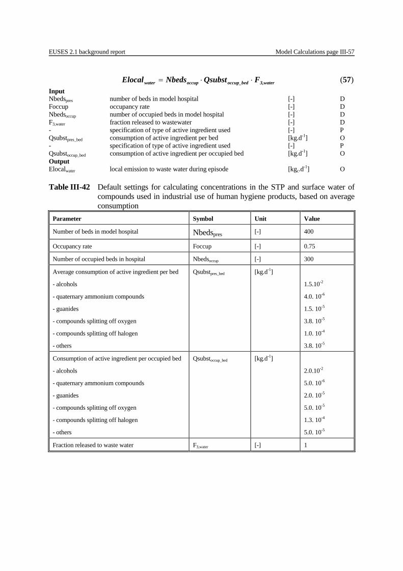
EUSES 2.1 background report Model Calculations page III-57
water3,occup_bedoccupwater FQsubstNbedsElocal ⋅⋅= (57) Input Nbedspres number of beds in model hospital [-] D Foccup occupancy rate [-] D Nbedsoccup number of occupied beds in model hospital [-] D F3,water fraction released to wastewater [-] D - specification of type of active ingredient used [-] P Qsubstpres_bed consumption of active ingredient per bed [kg.d-1] O - specification of type of active ingredient used [-] P Qsubstoccup_bed consumption of active ingredient per occupied bed [kg.d-1] O Output Elocalwater local emission to waste water during episode [kgc.d-1] O Table III-42 Default settings for calculating concentrations in the STP and surface water of
compounds used in industrial use of human hygiene products, based on average consumption
Parameter Symbol Unit Value
Number of beds in model hospital Nbedspres [-] 400
Occupancy rate Foccup [-] 0.75
Number of occupied beds in hospital Nbedsoccup [-] 300
Average consumption of active ingredient per bed
- alcohols
- quaternary ammonium compounds
- guanides
- compounds splitting off oxygen
- compounds splitting off halogen
- others
Qsubstpres_bed [kg.d-1]
1.5.10-2
4.0. 10-6
1.5. 10-5
3.8. 10-5
1.0. 10-4
3.8. 10-5
Consumption of active ingredient per occupied bed
- alcohols
- quaternary ammonium compounds
- guanides
- compounds splitting off oxygen
- compounds splitting off halogen
- others
Qsubstoccup_bed [kg.d-1]
2.0.10-2
5.0. 10-6
2.0. 10-5
5.0. 10-5
1.3. 10-4
5.0. 10-5
Fraction released to waste water F3,water [-] 1
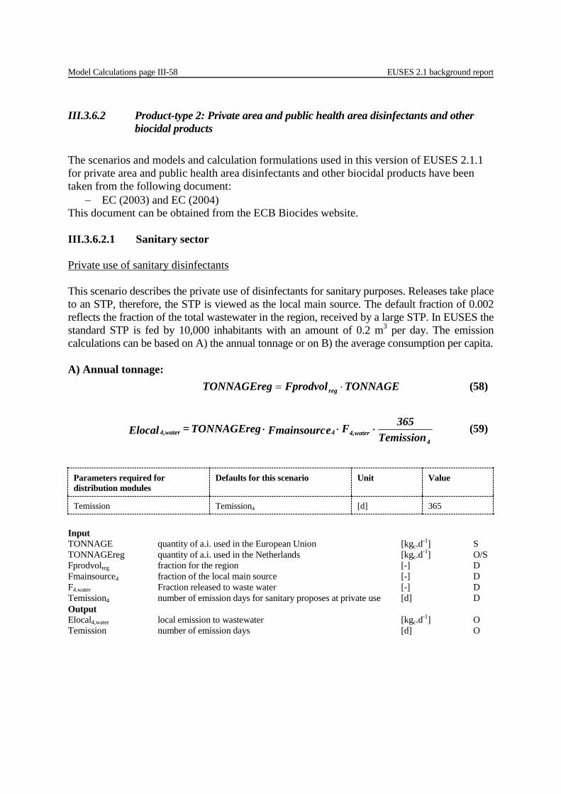
Model Calculations page III-58 EUSES 2.1 background report
III.3.6.2 Product-type 2: Private area and public health area disinfectants and other biocidal products The scenarios and models and calculation formulations used in this version of EUSES 2.1.1 for private area and public health area disinfectants and other biocidal products have been taken from the following document:
− EC (2003) and EC (2004) This document can be obtained from the ECB Biocides website. III.3.6.2.1 Sanitary sector Private use of sanitary disinfectants This scenario describes the private use of disinfectants for sanitary purposes. Releases take place to an STP, therefore, the STP is viewed as the local main source. The default fraction of 0.002 reflects the fraction of the total wastewater in the region, received by a large STP. In EUSES the standard STP is fed by 10,000 inhabitants with an amount of 0.2 m3 per day. The emission calculations can be based on A) the annual tonnage or on B) the average consumption per capita. A) Annual tonnage:
Parameters required for distribution modules
Defaults for this scenario Unit Value
Temission Temission4 [d] 365
Input TONNAGE quantity of a.i. used in the European Union [kgc.d-1] S TONNAGEreg quantity of a.i. used in the Netherlands [kgc.d-1] O/S Fprodvolreg fraction for the region [-] D Fmainsource4 fraction of the local main source [-] D F4.water Fraction released to waste water [-] D Temission4 number of emission days for sanitary proposes at private use [d] D Output Elocal4,water local emission to wastewater [kgc.d-1] O Temission number of emission days [d] O
TONNAGEFprodvolTONNAGEreg reg ⋅= (58)
4
water4,4water4, Temission365 F eFmainsourcTONNAGEreg= Elocal ⋅⋅⋅ (59)
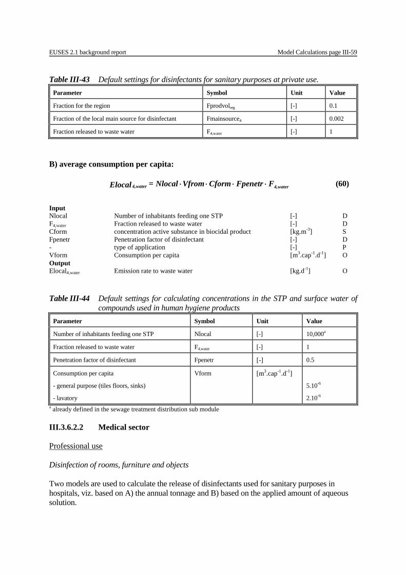
EUSES 2.1 background report Model Calculations page III-59
B) average consumption per capita: water4,water4, FFpenetrCform VfromNlocal= Elocal ⋅⋅⋅⋅ (60)
Input Nlocal Number of inhabitants feeding one STP [-] D F4,water Fraction released to waste water [-] D Cform concentration active substance in biocidal product [kg.m-3] S Fpenetr Penetration factor of disinfectant [-] D - type of application [-] P Vform Consumption per capita [m3.cap-1.d-1] O Output Elocal4,water Emission rate to waste water [kg.d-1] O Table III-44 Default settings for calculating concentrations in the STP and surface water of
compounds used in human hygiene products Parameter Symbol Unit Value
Number of inhabitants feeding one STP Nlocal [-] 10,000a
Fraction released to waste water F4,water [-] 1
Penetration factor of disinfectant Fpenetr [-] 0.5
Consumption per capita
- general purpose (tiles floors, sinks)
- lavatory
Vform [m3.cap-1.d-1]
5.10-6
2.10-6 a already defined in the sewage treatment distribution sub module III.3.6.2.2 Medical sector Professional use Disinfection of rooms, furniture and objects Two models are used to calculate the release of disinfectants used for sanitary purposes in hospitals, viz. based on A) the annual tonnage and B) based on the applied amount of aqueous solution.
Table III-43 Default settings for disinfectants for sanitary purposes at private use. Parameter Symbol Unit Value
Fraction for the region Fprodvolreg [-] 0.1
Fraction of the local main source for disinfectant Fmainsource4 [-] 0.002
Fraction released to waste water F4,water [-] 1
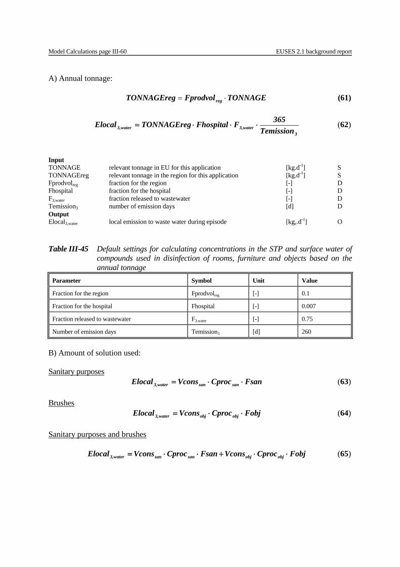
Model Calculations page III-60 EUSES 2.1 background report
A) Annual tonnage: TONNAGEFprodvolTONNAGEreg reg ⋅= (61)
3
water3,water3, Temission365FFhospitalTONNAGEregElocal ⋅⋅⋅= (62)
Input TONNAGE relevant tonnage in EU for this application [kg.d-1] S TONNAGEreg relevant tonnage in the region for this application [kg.d-1] S Fprodvolreg fraction for the region [-] D Fhospital fraction for the hospital [-] D F3,water fraction released to wastewater [-] D Temission3 number of emission days [d] D Output Elocal3,water local emission to waste water during episode [kgc.d-1] O Table III-45 Default settings for calculating concentrations in the STP and surface water of
compounds used in disinfection of rooms, furniture and objects based on the annual tonnage
Parameter Symbol Unit Value
Fraction for the region Fprodvolreg [-] 0.1
Fraction for the hospital Fhospital [-] 0.007
Fraction released to wastewater F3,water [-] 0.75
Number of emission days Temission3 [d] 260
B) Amount of solution used: Sanitary purposes FsanCprocVconsElocal sansanwater3, ⋅⋅= (63) Brushes FobjCprocVconsElocal objobjwater3, ⋅⋅= (64) Sanitary purposes and brushes FobjCprocVconsFsanCprocVconsElocal objobjsansanwater3, ⋅⋅+⋅⋅= (65)
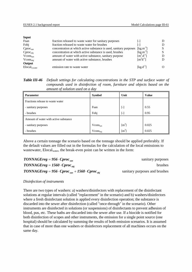
EUSES 2.1 background report Model Calculations page III-61
Input Fsan fraction released to waste water for sanitary purposes [-] D Fobj fraction released to waste water for brushes [-] D Cprocsan concentration at which active substance is used, sanitary purposes [kg.m-3] S Cprocobj concentration at which active substance is used, brushes [kg.m-3] S Vconssan amount of water with active substance, sanitary purpose [m3.d-1] D Vconsobj amount of water with active substance, brushes [m3d-1] D Output Elocal3,water emission rate to waste water [kg.d-1] O Table III-46 Default settings for calculating concentrations in the STP and surface water of
compounds used in disinfection of room, furniture and objects based on the amount of solution used on a day
Parameter Symbol Unit Value
Fractions release to waste water
- sanitary purposes
- brushes
Fsan
Fobj
[-]
[-]
0.55
0.95
Amount of water with active substance
- sanitary purposes
- brushes
Vconssan
Vconsobj
[m3]
[m3]
0.025
0.025
Above a certain tonnage the scenario based on the tonnage should be applied preferably. If the default values are filled out in the formulas for the calculation of the local emissions to wastewater, Elocalwater, the break-even point can be written in the form:
sanCproc956TONNAGEreg ⋅= sanitary purposes
objCproc1560TONNAGEreg ⋅= brushes
objsan Cproc1560Cproc956TONNAGEreg ⋅+⋅= sanitary purposes and brushes Disinfection of instruments There are two types of washers: a) washers/disinfectors with replacement of the disinfectant solutions at regular intervals (called "replacement" in the scenario) and b) washers/disinfectors where a fresh disinfectant solution is applied every disinfection operation; the substance is discarded into the sewer after disinfection (called "once-through" in the scenario). Other instruments are disinfected in solutions (or suspensions) of disinfectants to prevent adhesion of blood, pus, etc. These baths are discarded into the sewer after use. If a biocide is notified for both disinfection of scopes and other instruments, the emission for a single point source (one hospital) should be calculated by summing the results of both emission scenarios. It is assumed that in case of more than one washers or disinfectors replacement of all machines occurs on the same day.

Model Calculations page III-62 EUSES 2.1 background report
Washers or disinfectors, replacement: Concentration at day of replacement due to carry-over
replTintcarry_over
r)Fcarry_ove(1CprocCproc
+= (66)
Concentration at day of replacement including conversion repldisinf Tintkdeg
carry_overrepl eCprocCproc ⋅−⋅= (67) replmachwater3, CprocVprocNmaxElocal ⋅⋅= (68) Washers or disinfector, once through CprocVprocNmaxElocal machwater3, ⋅⋅= (69) Input Cproc working concentration of active ingredient [kg.m-3] S Nmaxmach number of washers or disinfectors [-] D - type of washer [-] P Vproc volume of solution in machine [m3] O Tintrepl Replacement interval [d] D Fcarry_over Fraction carry-over [-] D kdegdisinf Rate constant for chemical conversion [d-1] S/D
Output Elocal3,water emission rate to waste water [kg.d-1] O Table III-47 Default settings for calculating concentrations in the STP and surface water of
compounds used in disinfection of instruments with washers or disinfectors Parameter Symbol Unit Value
Maximum number of washers or disinfectors Nmaxmach [-] 3
Volume of solution in machine
- replacement
- once through
Vproc [m3]
0.1
0.01
Replacement interval (replacement) Tintrepl [d] 14
Fraction carry-over (replacement) Fcarry-over [-] 0.015
Rate constant for chemical conversion (replacement)
kdegdisinf [d-1] 0
Disinfection of instruments in baths: 0.5)ssionINT(1/TemiTint 3repl += (70)
repldisinf Tintkdeg
3water3, e
TemissionQsubstElocal ⋅−⋅= (71)
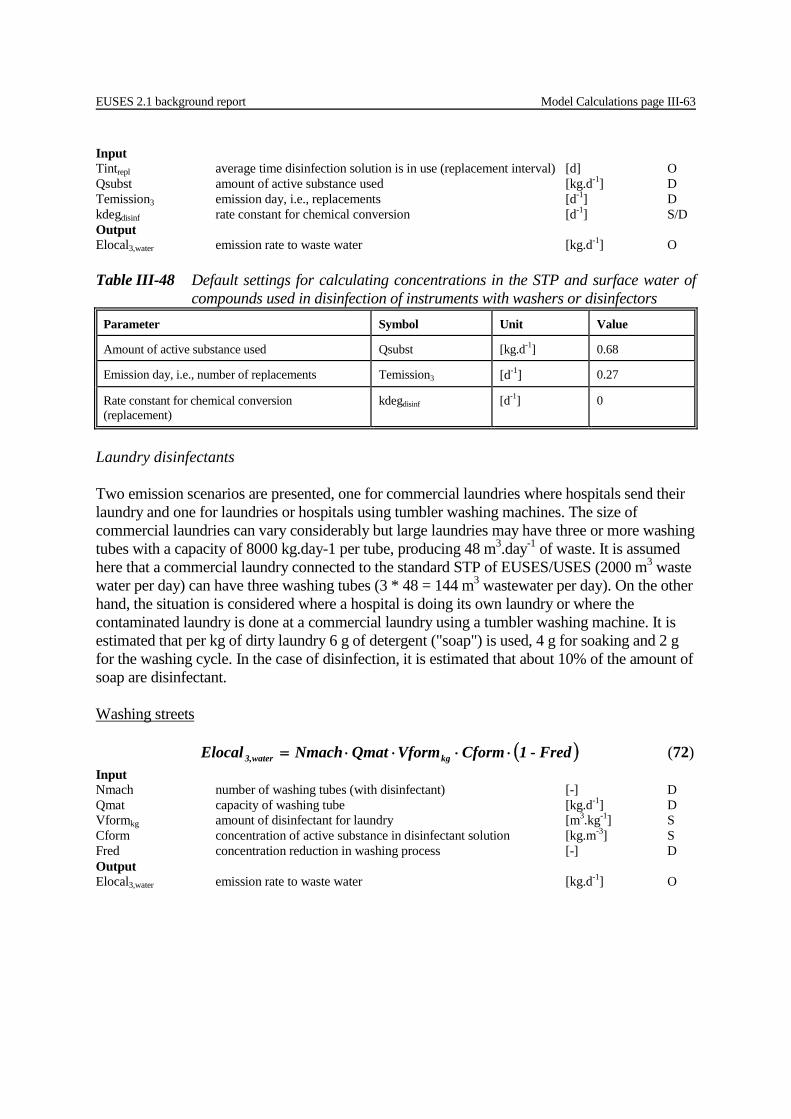
EUSES 2.1 background report Model Calculations page III-63
Input Tintrepl average time disinfection solution is in use (replacement interval) [d] O Qsubst amount of active substance used [kg.d-1] D Temission3 emission day, i.e., replacements [d-1] D kdegdisinf rate constant for chemical conversion [d-1] S/D
Output Elocal3,water emission rate to waste water [kg.d-1] O Table III-48 Default settings for calculating concentrations in the STP and surface water of
compounds used in disinfection of instruments with washers or disinfectors Parameter Symbol Unit Value
Amount of active substance used Qsubst [kg.d-1] 0.68
Emission day, i.e., number of replacements Temission3 [d-1] 0.27
Rate constant for chemical conversion (replacement)
kdegdisinf [d-1] 0
Laundry disinfectants Two emission scenarios are presented, one for commercial laundries where hospitals send their laundry and one for laundries or hospitals using tumbler washing machines. The size of commercial laundries can vary considerably but large laundries may have three or more washing tubes with a capacity of 8000 kg.day-1 per tube, producing 48 m3.day-1 of waste. It is assumed here that a commercial laundry connected to the standard STP of EUSES/USES (2000 m3 waste water per day) can have three washing tubes (3 * 48 = 144 m3 wastewater per day). On the other hand, the situation is considered where a hospital is doing its own laundry or where the contaminated laundry is done at a commercial laundry using a tumbler washing machine. It is estimated that per kg of dirty laundry 6 g of detergent ("soap") is used, 4 g for soaking and 2 g for the washing cycle. In the case of disinfection, it is estimated that about 10% of the amount of soap are disinfectant. Washing streets ( )Fred-1CformVformQmatNmachElocal kgwater3, ⋅⋅⋅⋅= (72) Input Nmach number of washing tubes (with disinfectant) [-] D Qmat capacity of washing tube [kg.d-1] D Vformkg amount of disinfectant for laundry [m3.kg-1] S Cform concentration of active substance in disinfectant solution [kg.m-3] S Fred concentration reduction in washing process [-] D Output Elocal3,water emission rate to waste water [kg.d-1] O
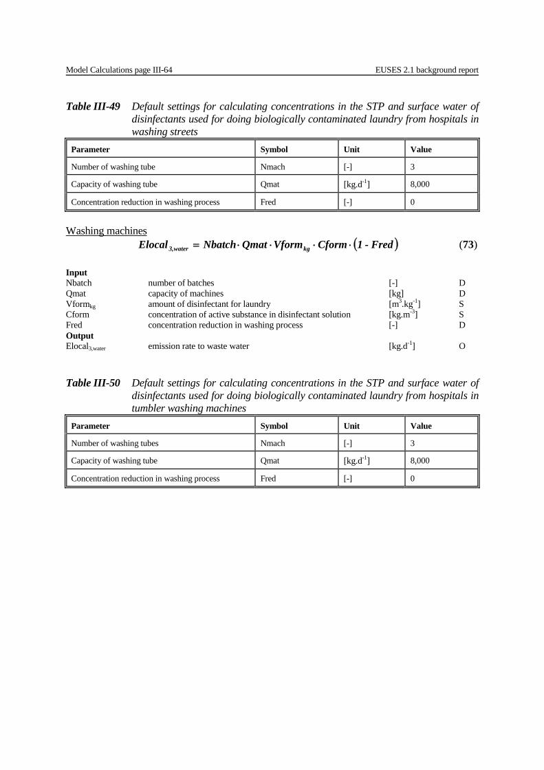
Model Calculations page III-64 EUSES 2.1 background report
Table III-49 Default settings for calculating concentrations in the STP and surface water of disinfectants used for doing biologically contaminated laundry from hospitals in washing streets
Parameter Symbol Unit Value
Number of washing tube Nmach [-] 3
Capacity of washing tube Qmat [kg.d-1] 8,000
Concentration reduction in washing process Fred [-] 0
Washing machines ( )Fred-1CformVformQmatNbatchElocal kgwater3, ⋅⋅⋅⋅= (73) Input Nbatch number of batches [-] D Qmat capacity of machines [kg] D Vformkg amount of disinfectant for laundry [m3.kg-1] S Cform concentration of active substance in disinfectant solution [kg.m-3] S Fred concentration reduction in washing process [-] D Output Elocal3,water emission rate to waste water [kg.d-1] O Table III-50 Default settings for calculating concentrations in the STP and surface water of
disinfectants used for doing biologically contaminated laundry from hospitals in tumbler washing machines
Parameter Symbol Unit Value
Number of washing tubes Nmach [-] 3
Capacity of washing tube Qmat [kg.d-1] 8,000
Concentration reduction in washing process Fred [-] 0
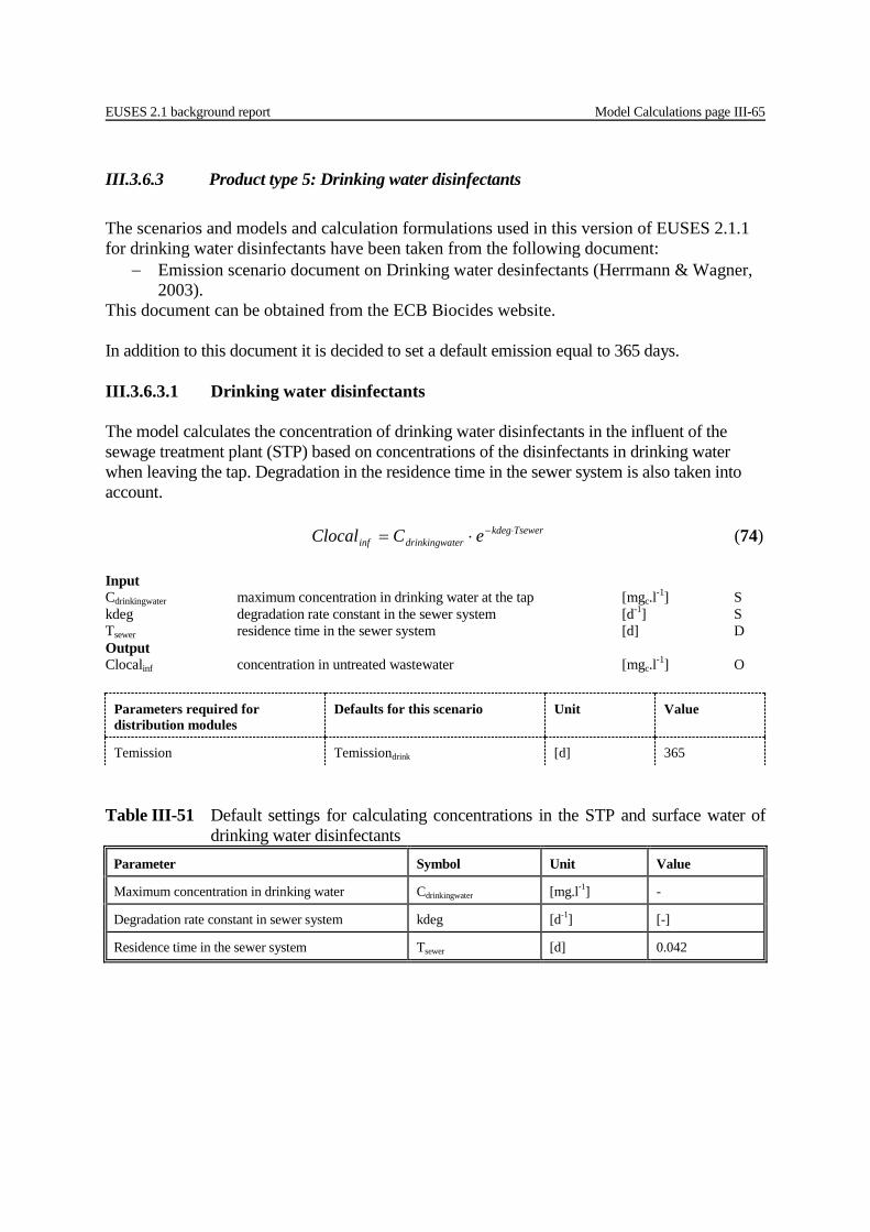
EUSES 2.1 background report Model Calculations page III-65
III.3.6.3 Product type 5: Drinking water disinfectants The scenarios and models and calculation formulations used in this version of EUSES 2.1.1 for drinking water disinfectants have been taken from the following document:
− Emission scenario document on Drinking water desinfectants (Herrmann & Wagner, 2003).
This document can be obtained from the ECB Biocides website. In addition to this document it is decided to set a default emission equal to 365 days. III.3.6.3.1 Drinking water disinfectants The model calculates the concentration of drinking water disinfectants in the influent of the sewage treatment plant (STP) based on concentrations of the disinfectants in drinking water when leaving the tap. Degradation in the residence time in the sewer system is also taken into account. Tsewerkdeg
terdrinkingwainf eCClocal ⋅−⋅= (74) Input Cdrinkingwater maximum concentration in drinking water at the tap [mgc.l-1] S kdeg degradation rate constant in the sewer system [d-1] S Tsewer residence time in the sewer system [d] D Output Clocalinf concentration in untreated wastewater [mgc.l-1] O
Parameters required for distribution modules
Defaults for this scenario Unit Value
Temission Temissiondrink [d] 365
Table III-51 Default settings for calculating concentrations in the STP and surface water of
drinking water disinfectants Parameter Symbol Unit Value
Maximum concentration in drinking water Cdrinkingwater [mg.l-1] -
Degradation rate constant in sewer system kdeg [d-1] [-]
Residence time in the sewer system Tsewer [d] 0.042
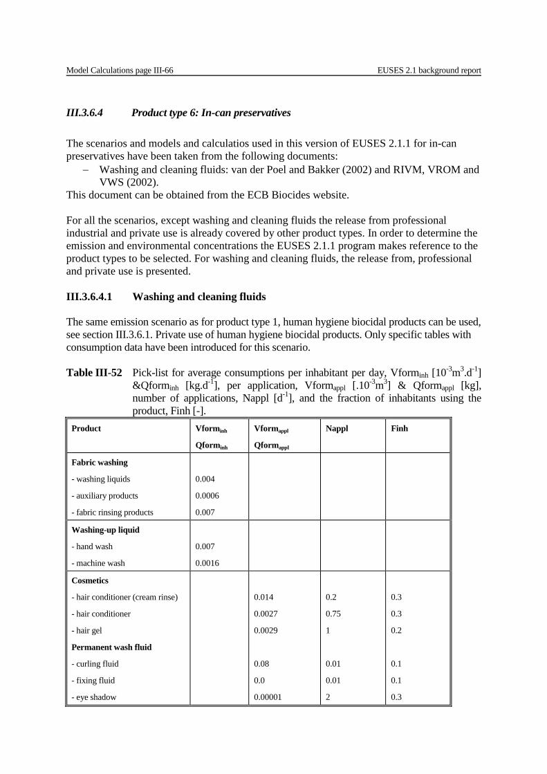
Model Calculations page III-66 EUSES 2.1 background report
III.3.6.4 Product type 6: In-can preservatives The scenarios and models and calculatios used in this version of EUSES 2.1.1 for in-can preservatives have been taken from the following documents:
− Washing and cleaning fluids: van der Poel and Bakker (2002) and RIVM, VROM and VWS (2002).
This document can be obtained from the ECB Biocides website. For all the scenarios, except washing and cleaning fluids the release from professional industrial and private use is already covered by other product types. In order to determine the emission and environmental concentrations the EUSES 2.1.1 program makes reference to the product types to be selected. For washing and cleaning fluids, the release from, professional and private use is presented. III.3.6.4.1 Washing and cleaning fluids The same emission scenario as for product type 1, human hygiene biocidal products can be used, see section III.3.6.1. Private use of human hygiene biocidal products. Only specific tables with consumption data have been introduced for this scenario. Table III-52 Pick-list for average consumptions per inhabitant per day, Vforminh [10-3m3.d-1]
&Qforminh [kg.d-1], per application, Vformappl [.10-3m3] & Qformappl [kg], number of applications, Nappl [d-1], and the fraction of inhabitants using the product, Finh [-].
Product Vforminh
Qforminh
Vformappl
Qformappl
Nappl Finh
Fabric washing
- washing liquids
- auxiliary products
- fabric rinsing products
0.004
0.0006
0.007
Washing-up liquid
- hand wash
- machine wash
0.007
0.0016
Cosmetics
- hair conditioner (cream rinse)
- hair conditioner
- hair gel
Permanent wash fluid
- curling fluid
- fixing fluid
- eye shadow
0.014
0.0027
0.0029
0.08
0.0
0.00001
0.2
0.75
1
0.01
0.01
2
0.3
0.3
0.2
0.1
0.1
0.3
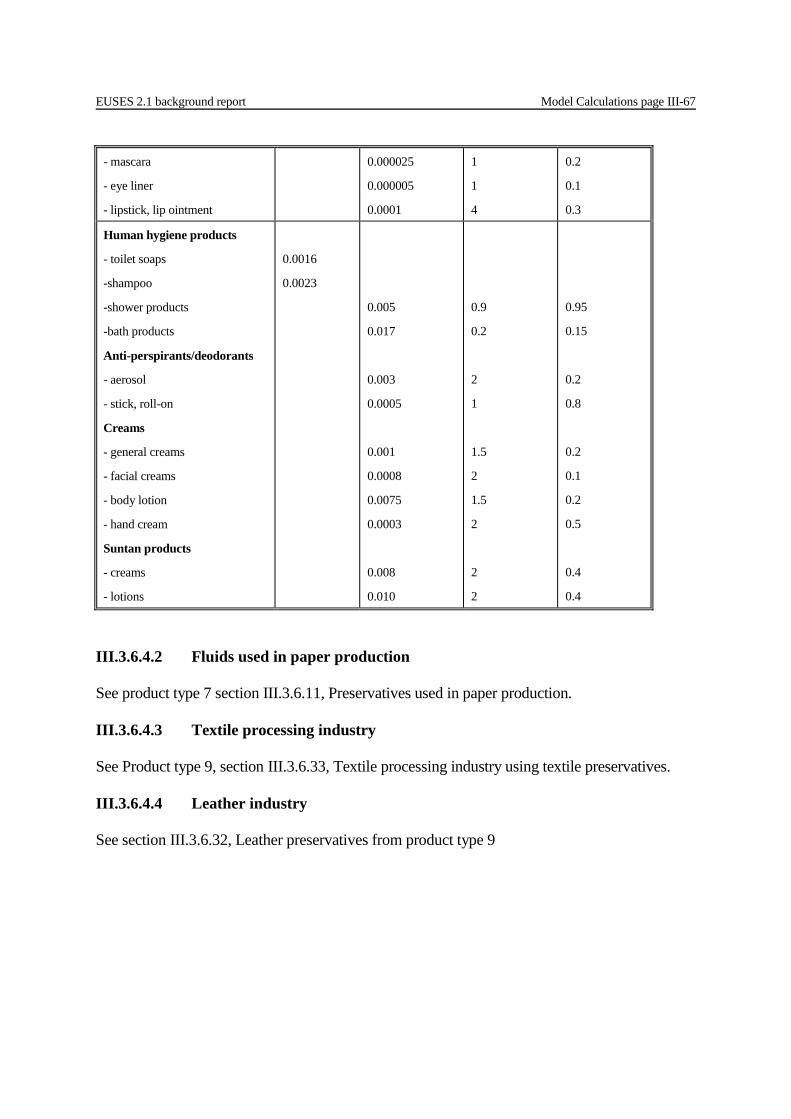
EUSES 2.1 background report Model Calculations page III-67
- mascara
- eye liner
- lipstick, lip ointment
0.000025
0.000005
0.0001
1
1
4
0.2
0.1
0.3
Human hygiene products
- toilet soaps
-shampoo
-shower products
-bath products
Anti-perspirants/deodorants
- aerosol
- stick, roll-on
Creams
- general creams
- facial creams
- body lotion
- hand cream
Suntan products
- creams
- lotions
0.0016
0.0023
0.005
0.017
0.003
0.0005
0.001
0.0008
0.0075
0.0003
0.008
0.010
0.9
0.2
2
1
1.5
2
1.5
2
2
2
0.95
0.15
0.2
0.8
0.2
0.1
0.2
0.5
0.4
0.4
III.3.6.4.2 Fluids used in paper production See product type 7 section III.3.6.11, Preservatives used in paper production. III.3.6.4.3 Textile processing industry See Product type 9, section III.3.6.33, Textile processing industry using textile preservatives. III.3.6.4.4 Leather industry See section III.3.6.32, Leather preservatives from product type 9

Model Calculations page III-68 EUSES 2.1 background report
III.3.6.5 Product type 7: Film preservatives The scenarios and models and calculation formulations used in this version of EUSES 2.1.1 for film preservatives have been taken from the following documents:
− Paints and coatings: supplement to the methodology for risk evaluation of biocides Environmental Emission Scenarios for biocides used as Film Preservatives (Product type 7) (European Commission DG ENV / RIVM, 2004)
− Pulp, paper and board industy (EC, 2004). This document can be obtained from the ECB Biocides website. III.3.6.5.1 Pulp, paper and board industry The emission scenario document comprises life cycle stages 3 (industrial use) and 6 (waste). For life cycle stage 3 the emission scenario calculates air releases from the drying sections after size-pressing and releases to wastewater from "broke" in the paper machine at stock preparation. For life cycle stage 6 the emission scenario calculates releases to wastewater resulting from paper recycling. The scenarios presented in this section are the same for in-can preservatives (PT 6) and fibre preservatives (PT 9). Life cycle stage Industrial use Releases from drying sections after size-pressing and coating
−
∆
⋅= 21 T1
T1
RH
T1T2 ePP (75) CformVformQsubst ⋅= (76) ( )Fdecomp1FevapQsubstQpaperElocal air3, −⋅⋅⋅= (77) Input Vform volume of product with preservative applied per kg of paper [m3.kg-1] S Cform concentration of active substance in the biocidal product [kgc.m-3] S Qsubst quantity of active substance applied per kg of paper [kgc.kg-1] S/O - type of paper produced [-] P Qpaper quantity of coated paper produced per day [kg.d-1] O PT1 vapour pressure at standard temperature [Pa] S PT2 vapour pressure at relevant application temperature [Pa] O ∆H heat of vaporisation for relevant temperature range [kJ.mol-1] S R universal gas constant [kJ.mol-1.K-1] D T1 standard temperature at which PT1 is measured [K] S T2 relevant application temperature [K] S Fevap fraction evaporated [-] O Output Elocal3,air local emission of active substance to air [kgc.d-1] O
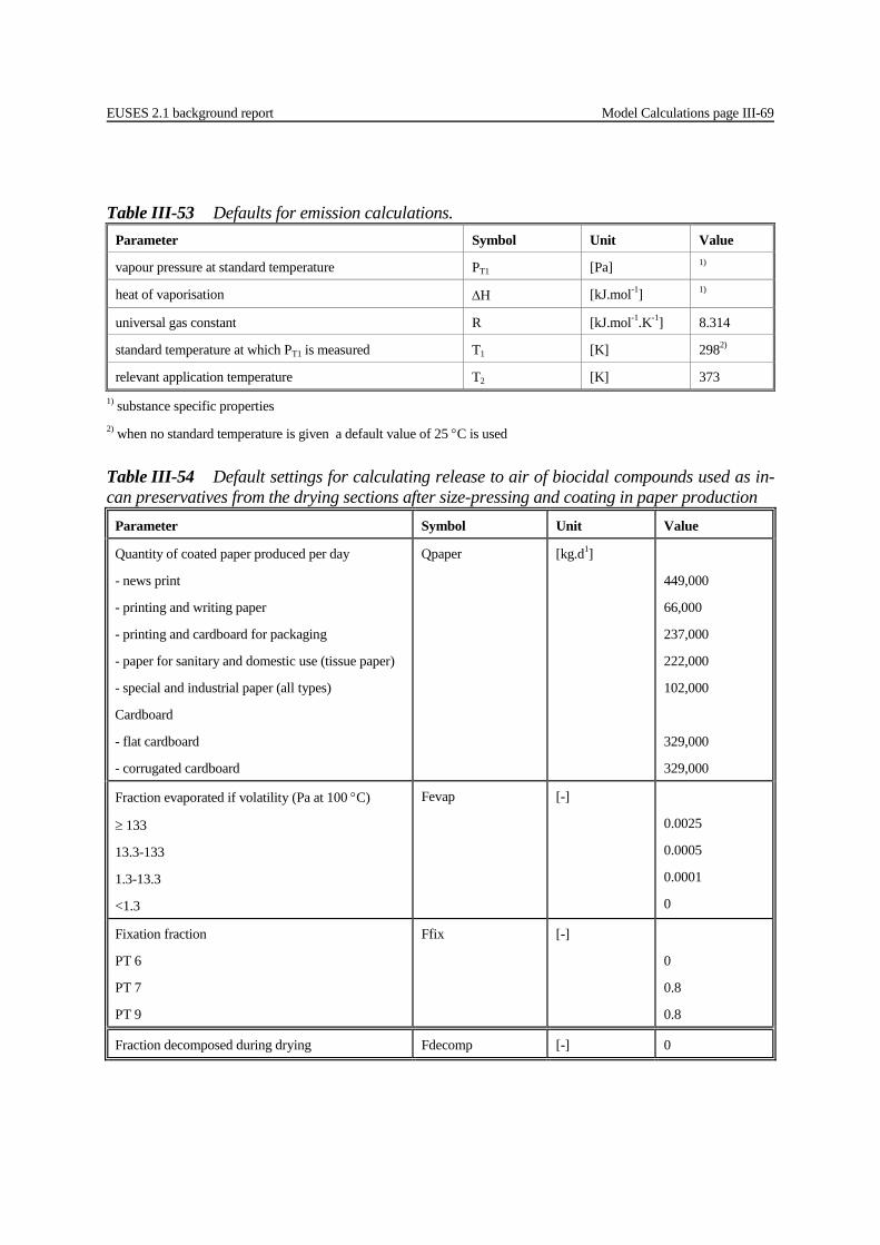
EUSES 2.1 background report Model Calculations page III-69
Table III-53 Defaults for emission calculations.
Parameter Symbol Unit Value
vapour pressure at standard temperature PT1 [Pa] 1)
heat of vaporisation ∆H [kJ.mol-1] 1)
universal gas constant R [kJ.mol-1.K-1] 8.314
standard temperature at which PT1 is measured T1 [K] 2982)
relevant application temperature T2 [K] 373 1) substance specific properties 2) when no standard temperature is given a default value of 25 °C is used
Table III-54 Default settings for calculating release to air of biocidal compounds used as in-can preservatives from the drying sections after size-pressing and coating in paper production
Parameter Symbol Unit Value
Quantity of coated paper produced per day
- news print
- printing and writing paper
- printing and cardboard for packaging
- paper for sanitary and domestic use (tissue paper)
- special and industrial paper (all types)
Cardboard
- flat cardboard
- corrugated cardboard
Qpaper [kg.d1]
449,000
66,000
237,000
222,000
102,000
329,000
329,000
Fraction evaporated if volatility (Pa at 100 °C)
≥ 133
13.3-133
1.3-13.3
<1.3
Fevap [-]
0.0025
0.0005
0.0001
0
Fixation fraction
PT 6
PT 7
PT 9
Ffix [-]
0
0.8
0.8
Fraction decomposed during drying Fdecomp [-] 0

Model Calculations page III-70 EUSES 2.1 background report
Releases from “broke” CformVformQsubst ⋅= (78) ( ) ( )Fclosure1Ffix1FbrokeQsubstQpaperElocal water3, −⋅−⋅⋅⋅= (79) Input Vform volume of product with preservative applied per kg of paper [m3.kg-1] S Cform concentration of active substance in the biocidal product [kgc.m-3] S Qsubst quantity of active substance applied per kg of paper [kgc.kg-1] S/O - type of paper produced [-] P Qpaper quantity of coated paper produced per day [kg.d-1] O Fbroke fraction of coated broke produced compared to overall production [-] D Ffix fixation fraction [-] D Fclosure degree of closure of the water system [-] O Output Elocal3,water local emission of active substance to waste water [kgc.d-1] O Table III-55 Default settings for calculating release to waste water of biocidal compounds
used as in-can preservatives from “broke” in paper production Parameter Symbol Unit Value
Degree of closure of the water system1)
- news print
- printing and writing paper
- printing and cardboard for packaging
- paper for sanitary and domestic use (tissue paper)
- special and industrial paper (all types)
Cardboard
- flat cardboard
- corrugated cardboard
Fclosure [-]
0.752)
0.553)
0.804)
0.752)
0.553)
0.804)
0.804)
Fraction of coated broke produced compared to overall production
Fbroke [-] 0.2
Fixation fraction Ffix [-] 0 1) the degree of closure will not effect the concentration of a substance in the wastewater, it will determine the volume of water and therefore the total amount of substance emitted. The wastewater flow should be adjusted accordingly when the degree of closure is changed. 2) a range of 0.65-0.85 was given in the ESD, 0.75 has been chosen as the average value 3) a range of 0.4-0.7 was given in the ESD, 0.55 has been chosen as the average value 4) a range of 0.65-0.95 and above was given in the ESD, 0.80 has been chosen as the average value
EUSES 2.1 background report Model Calculations page III-71
Life cycle stage waste treatment Paper recycling TONNAGEFprodvolTONNAGEreg reg ⋅= (80)
( ) ( )Nwdays
365Fdecomp1Fprelim-1
FdeinkeFmainsourcFrecTONNAGEregElocal 5water6,
⋅−⋅
⋅⋅⋅⋅= (81)
Input TONNAGE relevant tonnage in EU for this application [kg.d-1] S TONNAGEreg relevant tonnage in the region for this application [kg.d-1] S/O Fprodvolreg fraction for the region [-] D Fmainsource6 fraction of the main source (local STP) [-] D - type of paper recycled [-] P Frec fraction of paper recycled [-] O Fdeink fraction of preservatives released at de-inking [-] D Fdecomp fraction decomposed during de-inking [-] D - degree of solubility [-] P Fprelim fraction removed from waste water during preliminary [-] O on-site treatment Nwdays number of working days [d] D Output Elocal6,water local emission of active substance to waste water [kgc.d-1] O Table III-56 Default settings for calculating releases of in-can preservatives from paper
recycling Parameter Symbol Unit Value
Fraction for the region Fprovolreg [-] 0.1
Fraction of the main source Fmainsource6 [-] 0.1
Fraction of recycled paper
- news print
- printing and writing paper
- paper and cardboard for packaging
- paper for sanitary and domestic use (tissue paper)
- special and industrial paper (all types)
Cardboard
- flat cardboard
- corrugated cardboard
Frec [-] 0.54
0.58
0.11
0.46
0.54
0.55
0.92
0.90
Fraction of preservatives released at de-inking Fdeink [-] 1
Fraction decomposed during de-inking Fdecomp [-] 0
Fraction removed from wastewater during
preliminary on-site treatment
Fprelim
[-]
Model Calculations page III-72 EUSES 2.1 background report
Parameter Symbol Unit Value
- easy soluble1
- poorly soluble
0.1
0.7
Number of working days Nwdays [d] 340 1) Easy soluble substances are defined as having a water solubility >1000 mg.l-1. A range of 0-0.2 has been given in the ESD for easy soluble substance and a range of 0.5-0.9 has been reported for poorly soluble substances. III.3.6.5.2 Paints and coatings Formulation For emissions of biocides used as film preservatives the default A- and B-tables or the emission scenario document (ESD) from the TGD (2003) can be used for IC 14 Paints, lacquers and varnished industry, see also product type 6 section III.3.6.7, Paints and coatings. Private and proffesional use, sevice life and waste Film preservatives are only present in decorative paints, which are used by the public at large or professional painters. Thus paint application may be carried out by public at large and professionals at a relatively small scale. Paints may be applied, for example, by brush, rollers or spraying and will vary depending on the way of application and. As paint application is not a typical biocide application no emission scenarios have been developed specifically. For emission estimation the scenarios for new and existing substances may be applied. In the EA-UK document (EA-UK, 2002) an emission scenario document is found for industrial category 14 (Paints, lacquers and varnishes industry). Emission factors for decorative paint types are presented for the use of coatings (private and professional use) and also covers disposal of the coated product or removed paint (waste stage). The emission factors presented refer only to solids. Emissions are determined analogous to the stage of formulation as are the fraction of the main source and number of emission days. The calculations present the emission on the regional scale as a fraction of the regional tonnage. The local scale can be modelled starting from the sewage treatment plant (STP). Regional emissions are calculated for as wel water, soil and waste in the original ESD. For the exposure to biocides the emissions on the regional scale seem not to be the most relevant though. For this reason the regional release is no considered in EUSES 2.1. Furthermore, the relase to waste is not a standard compartment in EUSES. ntTONNAGEpaiFTONNAGE a.i. ⋅= (82) TONNAGEFprodvolTONNAGEreg reg ⋅= (83)
3
water3,3water Temission365FeFmainsourcTONNAGEregElocal ⋅⋅⋅= (84)

EUSES 2.1 background report Model Calculations page III-73
Input TONNAGEpaint tonnage of paint used in the EU containing the preservative [kg.d-1] S Fa.i. Fraction of the film preservative in the product [-] D TONNAGE relevant tonnage in EU for this application [kg.d-1] S TONNAGEreg relevant tonnage in the region for this application [kg.d-1] S/O Fprodvolreg fraction for the region [-] D Fmainsource3 fraction of the main source [-] O Temission3 number of emission days [d] O F3,water fraction released to wastewater during application [-] D F3,waste fraction released to waste during application [-] D F4,soil fraction released to soil during service life [-] D F5,waste fraction released to waste during removal [-] D Output Elocalwater local emission to water [kgc.d-1] O Table III-57 Default settings for calculating concentrations of film preservatives used in
coating products Parameter Symbol Unit Value
Fraction of the film preservative in the paint Fa.i. [-] 0.01
Fraction for the region Fprodvolreg [-] 0.1
Table III-58 Emission factors to air F3,air and (waste)water F3,water for the application of
decorative paint and coating products that are likely to contain film preservatives.
Parameter Symbol Unit Value
private professional
Fraction released to water during application F3,water [-] 0.03 0
Fraction disposed of as waste during application F3,waste [-] 0.25 0.07
Fraction to soil from paint during service life F4,soil [-] 0.02 0.03
Fraction disposed of as waste at the end of life (waste stage)
F5,waste [-] 0.70 0.90
* assuming treatment of flue gasses (0.98 if no treatment) Table III-59 Fraction of the main source, Fmainsource3 [-], and the number of emission days,
Temission3 [d], for the private and professional use of paints and coatings with in-can preservatives based on the corrected regional tonnage, TONNAGEregform [tonnes .yr-1], of the biocide
TONNAGEregform Fmainsource3 Temission3
< 500
≥500
0.002
0.002
150
300

Model Calculations page III-74 EUSES 2.1 background report
III.3.6.5.3 Polymers industry See section III.3.6.36, Polymerised materials preservatives under product type 9.

EUSES 2.1 background report Model Calculations page III-75
III.3.6.6 Product type 8: Wood preservatives and wood protectors The scenarios and models and calculation formulations used in this version of EUSES 2.1.1 for wood preservatives have been taken from the following document:
− OECD Series on Emission Scenario Documents. Number 2 Emission Scenario Document for Wood Preservatives Parts I to IV.
This document can be obtained from the ECB Biocides website and from the OECD. Since the ESD was first published discussions have taken place on a number of the parameters and the default values that have been included in the models.A number of recommendations for changing the default values have taken been made at Biocides Technical Meetings and then confirmed at Biocides Competent Authority meetings.Users of the EUSES 2.1.1 in the evaluation of wood preservatives (PT08) for the purposes of the Biocidal Products Directive (98/8/EC) should be aware that the default values included in the version they are using may not contain the latest decisions which have been made. Efforts should be made to obtain these and the ECB Biocides / COM should be approached for the latest values and insert them in their programme. It is envisaged that a formal procedure and documentary record of the decisions made on default values will be established. It is recommended that the user separately records in a table any changes made to the current default values used in the calculations for their risk assessments The following modifications have been made: Equation for calculating the volume of the soil compartment have been added. Furthermore the default value for the soil depth and distance from the source have been set to 0.5 m instead of the original value of 0.1 m. Industrial use III.3.6.6.1 Scenario for wood preservation through automated spraying Parameters/variables and default values for automated spraying.
Solid application rate: F Qform = Q iaia .... ⋅ (85)
Fluid application rate FRHOform Vform = Q iaia .... .⋅ (86)
( )driftairtreatedwoodiaair FF AREA Q = Elocal +⋅⋅ − ,3..,3 (87)
F AREA Q = Elocal watertreatedwoodiawater3 ,3.., ⋅⋅ − (88)
Model Calculations page III-76 EUSES 2.1 background report
Parameters required for distribution modules
Defaults for this scenario Unit Value
Temission Temission3 [d] 250
RIVERFLOW FLOWsurfacewater [m3.d-1] 25920 Input AREAwood-treated area of wood treated per day [m2.d-1] D VP vapour pressure [Pa] S SOL water solubility [kgc.m-3] S F3,air fraction released to air [-] Oc
F3,water fraction released to waste water [-] Oc Qform solid application rate of applied formulation [kg.m-2] S Vform fluid application rate of applied formulation [m3.m-2] S RHOproduct density of product [kg.m-3] S Fa.i. fraction of active ingredient in formulation [-] S Temission3 number of emission days for industrial use (including storage) [d] D Output Qa.i. quantity of active ingredient applied per m2 of wood [kg.m-2] S/O Elocal3,water local emission to waste water [kgc.d-1] O Elocal3,air local emission to air during episode [kgc.d-1] O
Table III-60 Default settings for automated spraying. Parameter Symbol Unit Value
Area of wood treated per day
small plants
large plants
AREAwood-treated [m2.d-1]
2 000
20 000
Quantity of active ingredient applied per unit of wood-area
Qai [kg.m-2] -
Fraction released to waste water Solubility in water [mg.m-3]
<0.25 0.25 – 1 1 – 50 50-100 ≥ 100
F3,water [-] 0.0001 0.0015 0.003 0.015 0.03
Fraction released to air Vapour pressure at 20 °C [Pa]
<0.005 0.005 - 0.05
0.05 - 0.5 0.5 - 1.25 1.25 - 2.5 ≥2.5
F3,air [-] 0.001 0.01 0.02 0.075 0.15 0.25
Fraction of spray drift Fdrift [-] 0.001

EUSES 2.1 background report Model Calculations page III-77
Parameters/variables and default values for storage at automated spraying facility. In the EUSES 2.1.1 program the concentration of substance in surface water after emissionof process water via STP and due to run-off are presented separately. The concentration in surface water after emission of process water via an STP is presented in the sheet on locan concentration and depositions.
stackedwood
treatedwoodstorage D
V Tstorage = AREA
−
−⋅ (89)
RHOsoilDEPTHsoil AREA = Qsoil storage ⋅⋅ (90)
FAREAAREA FLUX= Elocal runoffstorageexposedwoodstoragesoilstorage )1(, −⋅⋅⋅ − (91)
Qsoil
Temission Elocal = Csoil inisoilstorage
ini
⋅, (92)
Qsoil
Temission Elocal = Csoil chronsoilstorage
chron
⋅, (93)
runoffstorageexposedwoodstoragewaterstorage FAREAAREA FLUX = Elocal ⋅⋅ − ., (94)
ersurfacewat
water,storageoffrun FLOW
Elocal = Cwater − (95)
ersurfacewat
stpefferprocesswat FLOW
calEFFLUENTloClocal = Cwater
⋅ (96)
ersurfacewat
stpeff
ersurfacewat
water,storagetotal FLOW
calEFFLUENTloClocalFLOWElocal
= Cwater⋅
+ (97)
Model Calculations page III-78 EUSES 2.1 background report
Input Tstorage duration of storage of treated wood prior to shipment [d] D Vwood-treated volume of wood treated per day [m3.d-1] D Dwood-stacked storage density of treated wood stacked on storage area [m3.m-2] D DEPTHsoil depth of soil [m] D RHOsoil wet soil bulk density [kgwwt.m-3] Oc
FLUXstorage average daily flux of the a.i during the storage period [kgc.m-2.d-1] S AREAwood-exposed effective surface area of treated wood exposed to rain per unit of storage area [m2.m-2] D Frunoff fraction of rainwater running off the storage site [-] D Elocalstroage,soil local emission to soil from storage [kgc.d-1] O Temissionini duration of the initial assessment period [d] D Temissionchron duration of the chronic assesssment period [d] S FLOWsurfacewater volume flow rate of creek/river [m3.d-1] D Clocaleff sewage treatment plant effluent concentration (EUSES output) [kgc.m-3] Oc
EFFLUENTlocalstp effluent flow of the local sewage treatment plant [m3.d-1] Oc AREAstorage surface area of the storage place [m2] D/O Output Qsoil wet soil mass [kgwwt] O Elocal3,air local emission to air [kgc.d-1] O Elocal3, water local emission to surface water [kgc.d-1] O Elocalstorage, water local emission to surface water from storage [kgc.d-1] O Csoilini concentration of substance in soil for initial assessment period [kgc.kg-1
wwt] O Csoilchron concentration of substance in soil for longer assessment period [kgc.kg-1
wwt] O Cwaterprocess water concentration of substance in surface water after emission of process water via STP [kgc.m-3] O Cwaterrun-off concentration of substance in surface water due to run-off [kgc.m-3] O Cwatertotal concentration of substance in surface water [kgc.m-3] O
Table III-61 Default settings for storage site at automated spraying facility. Parameter Symbol Unit Value
Duration of storage of treated wood prior to shipment Tstorage [d] 3
Volume of wood treated per day
small company
large company
Vwood-treated
[m3.d-1]
52,5
525
Storage density of treated wood on storage area Dwood-stacked [m3.m-2] 2
Depth of soil DEPTHsoil [m] 0.5
Wet soil bulk density RHOsoil [kgwwt.m3] 1700
Average daily flux of the active ingredient during storage period
FLUXstorage [kgc.m-2.d-1] -
Effective surface area of treated wood exposed to rain per unit of storage area
AREAwood-exposed [m2.m-2] 11
Fraction of rain water running of storage area Frunoff [-] 0.5
Duration of the initial assessment period Temissionini [d] 30
Duration of the chronic assessment period Temisisionchron [d] >30
Volume flow rate of creek FLOWcreek [m3.d-1] 25 920
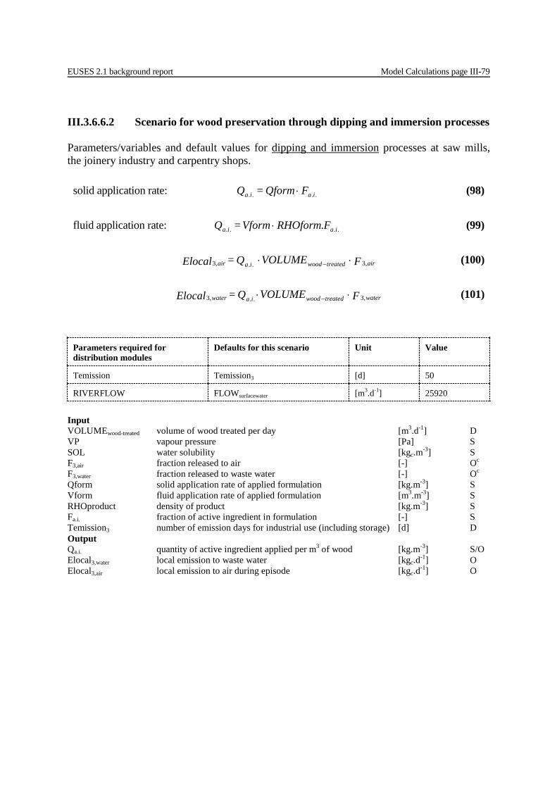
EUSES 2.1 background report Model Calculations page III-79
III.3.6.6.2 Scenario for wood preservation through dipping and immersion processes Parameters/variables and default values for dipping and immersion processes at saw mills, the joinery industry and carpentry shops.
Parameters required for distribution modules
Defaults for this scenario Unit Value
Temission Temission3 [d] 50
RIVERFLOW FLOWsurfacewater [m3.d-1] 25920
Input VOLUMEwood-treated volume of wood treated per day [m3.d-1] D VP vapour pressure [Pa] S SOL water solubility [kgc.m-3] S F3,air fraction released to air [-] Oc
F3,water fraction released to waste water [-] Oc Qform solid application rate of applied formulation [kg.m-3] S Vform fluid application rate of applied formulation [m3.m-3] S RHOproduct density of product [kg.m-3] S Fa.i. fraction of active ingredient in formulation [-] S Temission3 number of emission days for industrial use (including storage) [d] D Output Qa.i. quantity of active ingredient applied per m3 of wood [kg.m-3] S/O Elocal3,water local emission to waste water [kgc.d-1] O Elocal3,air local emission to air during episode [kgc.d-1] O
solid application rate: F Qform = Q iaia .... ⋅ (98)
fluid application rate: FRHOform Vform = Q iaia .... .⋅ (99)
F VOLUME Q = Elocal airtreatedwoodiaair ,3..,3 ⋅⋅ − (100)
F VOLUME Q = Elocal watertreatedwoodiawater ,3..,3 ⋅⋅ − (101)
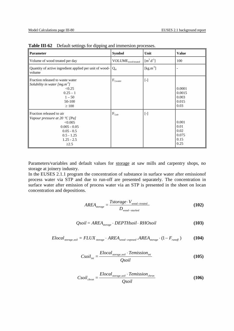
Model Calculations page III-80 EUSES 2.1 background report
Parameters/variables and default values for storage at saw mills and carpentry shops, no storage at joinery industry. In the EUSES 2.1.1 program the concentration of substance in surface water after emissionof process water via STP and due to run-off are presented separately. The concentration in surface water after emission of process water via an STP is presented in the sheet on locan concentration and depositions.
Table III-62 Default settings for dipping and immersion processes. Parameter Symbol Unit Value
Volume of wood treated per day VOLUMEwood-treated [m3.d-1] 100
Quantity of active ingredient applied per unit of wood-volume
Qai [kg.m-3] -
Fraction released to waste water Solubility in water [mg.m-3]
<0.25 0.25 – 1 1 – 50 50-100 ≥ 100
F3,water [-] 0.0001 0.0015 0.003 0.015 0.03
Fraction released to air Vapour pressure at 20 °C [Pa]
<0.005 0.005 - 0.05
0.05 - 0.5 0.5 - 1.25 1.25 - 2.5 ≥2.5
F3,air [-] 0.001 0.01 0.02 0.075 0.15 0.25
stackedwood
treatedwoodstorage D
V Tstorage = AREA
−
−⋅ (102)
RHOsoilDEPTHsoil AREA = Qsoil storage ⋅⋅ (103)
FAREAAREA FLUX= Elocal runoffstorageexposedwoodstoragesoilstorage )1(., −⋅⋅ − (104)
Qsoil
Temission Elocal = Csoil inisoilstorage
ini
⋅, (105)
Qsoil
Temission Elocal = Csoil chronsoilstorage
chron
⋅, (106)
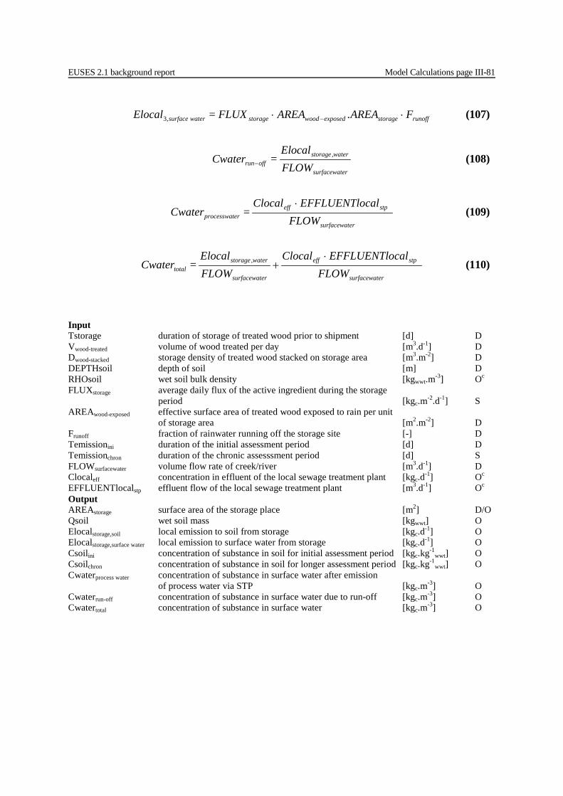
EUSES 2.1 background report Model Calculations page III-81
Input Tstorage duration of storage of treated wood prior to shipment [d] D Vwood-treated volume of wood treated per day [m3.d-1] D Dwood-stacked storage density of treated wood stacked on storage area [m3.m-2] D DEPTHsoil depth of soil [m] D RHOsoil wet soil bulk density [kgwwt.m-3] Oc
FLUXstorage average daily flux of the active ingredient during the storage period [kgc.m-2.d-1] S AREAwood-exposed effective surface area of treated wood exposed to rain per unit of storage area [m2.m-2] D Frunoff fraction of rainwater running off the storage site [-] D Temissionini duration of the initial assessment period [d] D Temissionchron duration of the chronic assesssment period [d] S FLOWsurfacewater volume flow rate of creek/river [m3.d-1] D Clocaleff concentration in effluent of the local sewage treatment plant [kgc.d-1] Oc EFFLUENTlocalstp effluent flow of the local sewage treatment plant [m3.d-1] Oc
Output AREAstorage surface area of the storage place [m2] D/O Qsoil wet soil mass [kgwwt] O Elocalstorage,soil local emission to soil from storage [kgc.d-1] O Elocalstorage,surface water local emission to surface water from storage [kgc.d-1] O Csoilini concentration of substance in soil for initial assessment period [kgc.kg-1
wwt] O Csoilchron concentration of substance in soil for longer assessment period [kgc.kg-1
wwt] O Cwaterprocess water concentration of substance in surface water after emission of process water via STP [kgc.m-3] O Cwaterrun-off concentration of substance in surface water due to run-off [kgc.m-3] O Cwatertotal concentration of substance in surface water [kgc.m-3] O
runoffstorageexposedwoodstoragewatersurface FAREAAREA FLUX = Elocal ⋅⋅ − .,3 (107)
ersurfacewat
water,storageoffrun FLOW
Elocal = Cwater − (108)
ersurfacewat
stpefferprocesswat FLOW
calEFFLUENTloClocal = Cwater
⋅ (109)
ersurfacewat
stpeff
ersurfacewat
water,storagetotal FLOW
calEFFLUENTloClocalFLOWElocal
= Cwater⋅
+ (110)
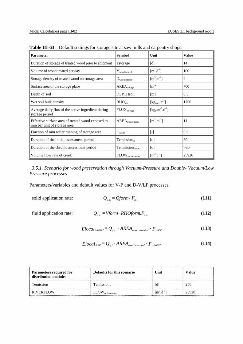
Model Calculations page III-82 EUSES 2.1 background report
.3.5.1. Scenario for wood preservation through Vacuum-Pressure and Double- Vacuum/Low Pressure processes Parameters/variables and default values for V-P and D-V/LP processes.
Parameters required for distribution modules
Defaults for this scenario Unit Value
Temission Temission3 [d] 250
RIVERFLOW FLOWsurfacewater [m3.d-1] 25920
Table III-63 Default settings for storage site at saw mills and carpentry shops. Parameter Symbol Unit Value
Duration of storage of treated wood prior to shipment Tstorage [d] 14
Volume of wood treated per day Vwood-treated [m3.d-1] 100
Storage density of treated wood on storage area Dwood-stacked [m3.m-2] 2
Surface area of the storage place AREAstorage [m-2] 700
Depth of soil DEPTHsoil [m] 0.5
Wet soil bulk density RHOsoil [kgwwt.m3] 1700
Average daily flux of the active ingredient during storage period
FLUXstorage [kgc.m-2.d-1] -
Effective surface area of treated wood exposed to rain per unit of storage area
AREAwood-leach [m2.m-2] 11
Fraction of rain water running of storage area Frunoff [-] 0.5
Duration of the initial assessment period Temissionini [d] 30
Duration of the chronic assessment period Temisisionchron [d] >30
Volume flow rate of creek FLOWsurfacewater [m3.d-1] 25920
solid application rate: F Qform = Q iaia .... ⋅ (111)
fluid application rate: FRHOform Vform = Q iaia .... .⋅ (112)
F AREA Q = Elocal airtreatedwoodiawater ,3..,3 ⋅⋅ − (113)
F AREA Q = Elocal watertreatedwoodiaair ,3..,3 ⋅⋅ − (114)
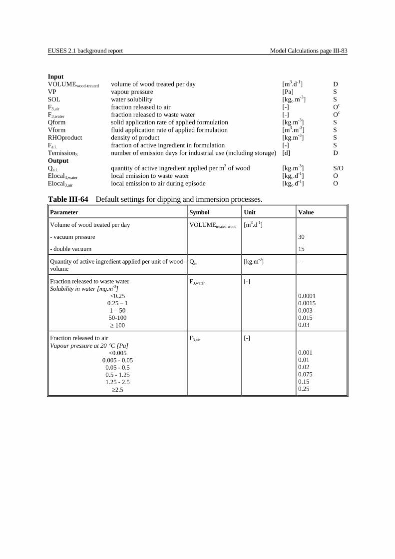
EUSES 2.1 background report Model Calculations page III-83
Input VOLUMEwood-treated volume of wood treated per day [m3.d-1] D VP vapour pressure [Pa] S SOL water solubility [kgc.m-3] S F3,air fraction released to air [-] Oc
F3,water fraction released to waste water [-] Oc Qform solid application rate of applied formulation [kg.m-3] S Vform fluid application rate of applied formulation [m3.m-3] S RHOproduct density of product [kg.m-3] S Fa.i. fraction of active ingredient in formulation [-] S Temission3 number of emission days for industrial use (including storage) [d] D Output Qa.i. quantity of active ingredient applied per m3 of wood [kg.m-3] S/O Elocal3,water local emission to waste water [kgc.d-1] O Elocal3,air local emission to air during episode [kgc.d-1] O
Table III-64 Default settings for dipping and immersion processes. Parameter Symbol Unit Value
Volume of wood treated per day
- vacuum pressure
- double vacuum
VOLUMEtreated-wood [m3.d-1]
30
15
Quantity of active ingredient applied per unit of wood-volume
Qai [kg.m-3] -
Fraction released to waste water Solubility in water [mg.m-3]
<0.25 0.25 – 1 1 – 50 50-100 ≥ 100
F3,water [-] 0.0001 0.0015 0.003 0.015 0.03
Fraction released to air Vapour pressure at 20 °C [Pa]
<0.005 0.005 - 0.05
0.05 - 0.5 0.5 - 1.25 1.25 - 2.5 ≥2.5
F3,air [-] 0.001 0.01 0.02 0.075 0.15 0.25

Model Calculations page III-84 EUSES 2.1 background report
Parameters/variables and default values for storage at vacuum-pressure treatment. In the EUSES 2.1.1 program the concentration of substance in surface water after emissionof process water via STP and due to run-off are presented separately. The concentration in surface water after emission of process water via an STP is presented in the sheet on locan concentration and depositions.
stackedwood
treatedwoodstorage D
V Tstorage = AREA
−
−⋅ (115)
RHOsoilDEPTHsoil AREA = Qsoil storage ⋅⋅ (116)
FAREAAREA FLUX= Elocal runoffstorageexposedwoodstoragesoilstorage )1(., −⋅⋅ − (117)
Qsoil
Temission Elocal = Csoil inisoilstorage
ini
⋅, (118)
Qsoil
Temission Elocal = Csoil chronsoilstorage
chron
⋅, (119)
runoffstorageexposedwoodstoragewatersurface FAREAAREA FLUX = Elocal ⋅⋅ − .,3 (120)
ersurfacewat
water,storageoffrun FLOW
Elocal = Cwater − (121)
ersurfacewat
stpefferprocesswat FLOW
calEFFLUENTloClocal = Cwater
⋅ (122)
ersurfacewat
stpeff
ersurfacewat
water,storagetotal FLOW
calEFFLUENTloClocalFLOWElocal
= Cwater⋅
+ (123)

EUSES 2.1 background report Model Calculations page III-85
Input Tstorage duration of storage of treated wood prior to shipment [d] D Vwood-treated volume of wood treated per day [m3.d-1] D Dwood-stacked storage density of treated wood stacked on storage area [m3.m-2] D DEPTHsoil depth of soil [m] D RHOsoil wet soil bulk density [kgwwt.m-3] Oc
FLUXstorage average daily flux of the active ingredient during the storage period [kgc.m-2.d-1] S AREAwood-exposed effective surface area of treated wood exposed to rain per unit of storage area [m2.m-2] D Frunoff fraction of rainwater running off the storage site [-] D Temissionini duration of the initial assessment period [d] D Temissionchron duration of the chronic assesssment period [d] S Clcoaleff local treatment plant effluent concentration [kgc.m-3] Oc EFFLUENTlocalstp effluent flow of the local sewage treatment plant [m3.d-1] Oc FLOWsurfacewater volume flow rate of creek [m3.d-1] D Output AREAstorage surface area of the storage place [m2] D/O Qsoil wet soil mass [kgwwt] O Elocal3,soil local emission to soil from storage [kgc.d-1] O Elocal3,surface water local emission to surface water from storage [kgc.d-1] O Csoilini concentration of substance in soil for initial assessment period [kgc.kg-1
wwt] O Csoilchron concentration of substance in soil for longer assessment period [kgc.kg-1
wwt] O Cwaterprocess water concentration of substance in surface water after emission of process water via STP [kgc.m-3] O Cwaterrun-off concentration of substance in surface water due to run-off [kgc.m-3] O Cwatertotal concentration of substance in surface water [kgc.m-3] O
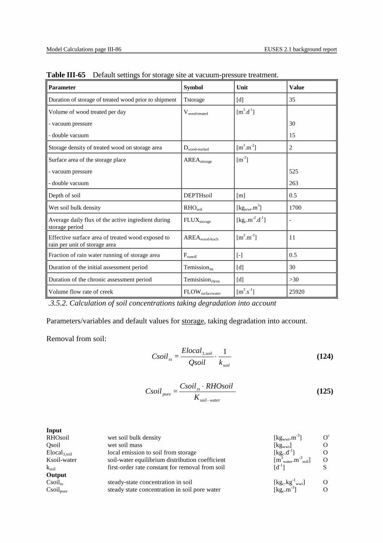
Model Calculations page III-86 EUSES 2.1 background report
.3.5.2. Calculation of soil concentrations taking degradation into account Parameters/variables and default values for storage, taking degradation into account. Removal from soil:
Input RHOsoil wet soil bulk density [kgwwt.m-3] Oc
Qsoil wet soil mass [kgwwt] O Elocal3,soil local emission to soil from storage [kgc.d-1] O Ksoil-water soil-water equilibrium distribution coefficient [m3
water.m-3soil] O
ksoil first-order rate constant for removal from soil [d-1] S Output Csoilss steady-state concentration in soil [kgc.kg-1
wwt] O Csoilpore steady state concentration in soil pore water [kgc.m-3] O
Table III-65 Default settings for storage site at vacuum-pressure treatment. Parameter Symbol Unit Value
Duration of storage of treated wood prior to shipment Tstorage [d] 35
Volume of wood treated per day
- vacuum pressure
- double vacuum
Vwood-treated [m3.d-1]
30
15
Storage density of treated wood on storage area Dwood-stacked [m3.m-2] 2
Surface area of the storage place
- vacuum pressure
- double vacuum
AREAsttorage [m-2]
525
263
Depth of soil DEPTHsoil [m] 0.5
Wet soil bulk density RHOsoil [kgwwt.m3] 1700
Average daily flux of the active ingredient during storage period
FLUXstorage [kgc.m-2.d-1] -
Effective surface area of treated wood exposed to rain per unit of storage area
AREAwood-leach [m2.m-2] 11
Fraction of rain water running of storage area Frunoff [-] 0.5
Duration of the initial assessment period Temissionini [d] 30
Duration of the chronic assessment period Temisisionchron [d] >30
Volume flow rate of creek FLOWsurfacewater [m3.s-1] 25920
soil
soilss k
Qsoil
Elocal = Csoil 1,3 ⋅ (124)
K
RHOsoilCsoil = Csoil
watersoil
sspore
−
⋅ (125)

EUSES 2.1 background report Model Calculations page III-87
Service Life III.3.6.6.3 Emissions from treated wood, scenario for a fence Parameters/variables and default values for a fence.
Parameters required for distribution modules
Defaults for this scenario Unit Value
Temission Temissionini [d] 30
Temission Temissionchron [d] >30
Input WIDTHsoil width of receiving soil [m] D DEPTHsoil depth of receiving soil [m] D Vsoil volume of soil [m3] O RHOsoil wet soil bulk density [kgwwt.m-3] D FLUXwood,ini average daily flux of the active ingredient over the initial assessment period [kgc.m-2.d-1] S FLUXwood,chron average daily flux of the active ingredient over the chronic assessment period [kgc.m-2.d-1] S AREAfence leachable wood area per unit of length of fence [m2] D Output Qsoil wet soil mass [kgwwt] O/S Qleachini average rate of active ingredient leached out of treated wood during the initial assessment period [kgc.d-1] O/S Qleachchron average rate of active ingredient leached out of treated wood during the chronic assessment period [kgc.d-1] O Csoilini concentration of substance in soil for initial assessment period [kgc.kg-1
wwt] O Csoilchron concentration of substance in soil for longer assessment period [kgc.kg-1
wwt] O
DEPTHsoilWIDTHsoil = Vsoil ⋅⋅1 (126)
RHOsoilVsoil = Qsoil ⋅ (127)
AREA FLUX= Qleach fenceiniwoodini ⋅, (128)
AREA FLUX= Qleach fencechronwoodchron ⋅, (129)
Qsoil
Temission Qleach = Csoil iniini
ini⋅ (130)
Qsoil
Temission Qleach = Csoil chronchron
chron⋅ (131)
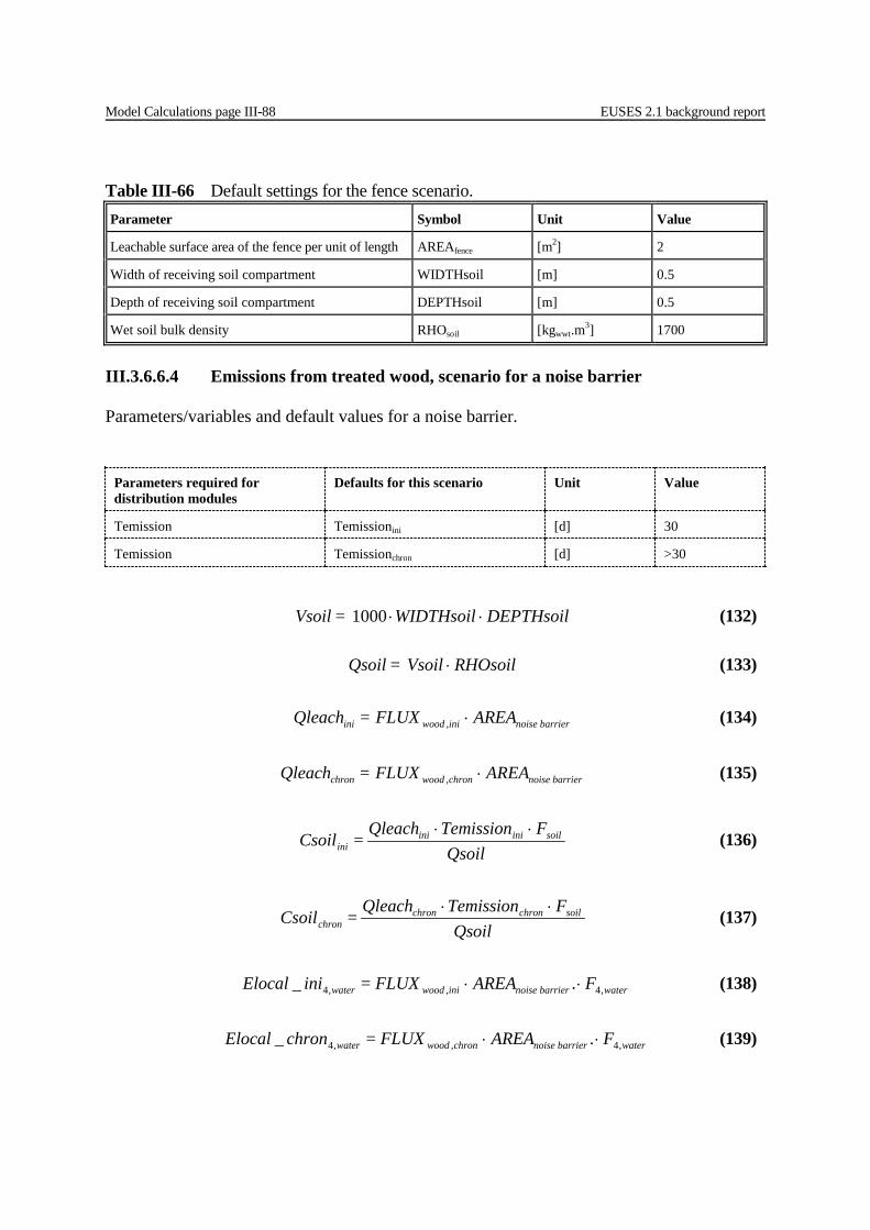
Model Calculations page III-88 EUSES 2.1 background report
III.3.6.6.4 Emissions from treated wood, scenario for a noise barrier Parameters/variables and default values for a noise barrier.
Parameters required for distribution modules
Defaults for this scenario Unit Value
Temission Temissionini [d] 30
Temission Temissionchron [d] >30
Table III-66 Default settings for the fence scenario. Parameter Symbol Unit Value
Leachable surface area of the fence per unit of length AREAfence [m2] 2
Width of receiving soil compartment WIDTHsoil [m] 0.5
Depth of receiving soil compartment DEPTHsoil [m] 0.5
Wet soil bulk density RHOsoil [kgwwt.m3] 1700
DEPTHsoilWIDTHsoil = Vsoil ⋅⋅1000 (132)
RHOsoilVsoil = Qsoil ⋅ (133)
AREA FLUX= Qleach barriernoiseiniwoodini ⋅, (134)
AREA FLUX= Qleach barriernoisechronwoodchron ⋅, (135)
Qsoil
FTemission Qleach = Csoil soiliniini
ini⋅⋅ (136)
Qsoil
FTemission Qleach = Csoil soilchronchron
chron⋅⋅ (137)
waterbarriernoiseiniwoodwater FAREA FLUX = iniElocal ,4,,4 ._ ⋅⋅ (138)
waterbarriernoisechronwoodwater FAREA FLUX = chronElocal ,4,,4 ._ ⋅⋅ (139)
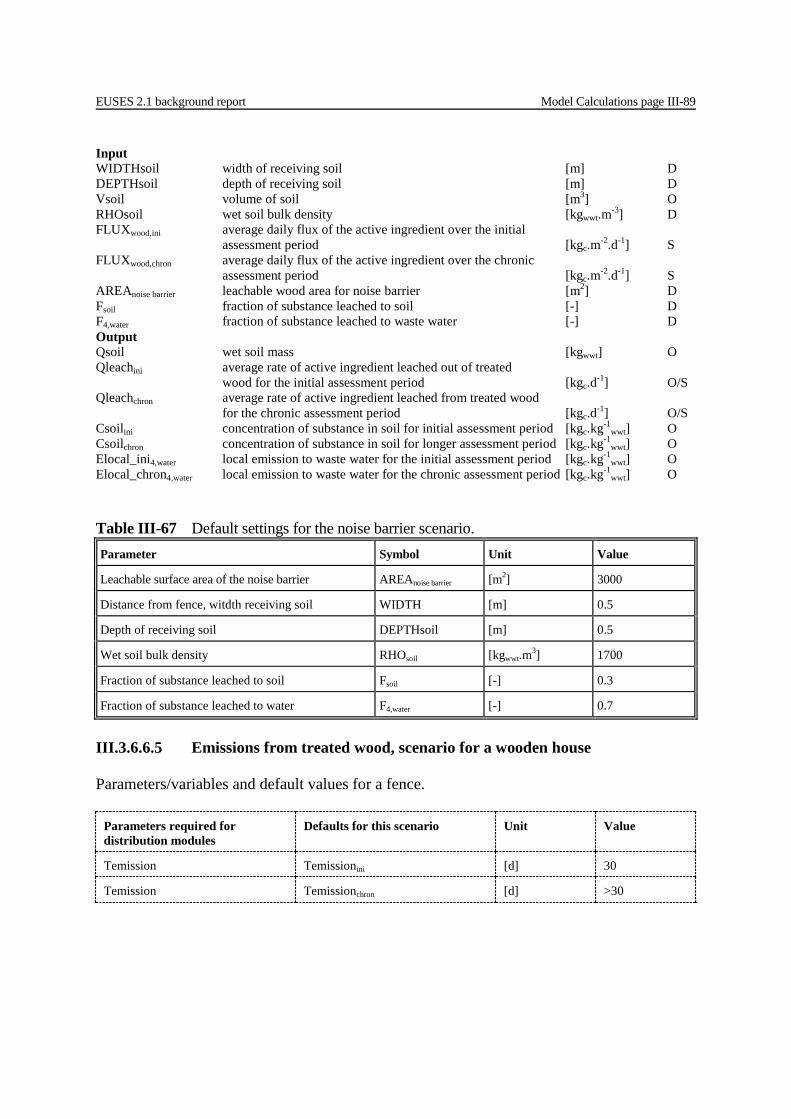
EUSES 2.1 background report Model Calculations page III-89
Input WIDTHsoil width of receiving soil [m] D DEPTHsoil depth of receiving soil [m] D Vsoil volume of soil [m3] O RHOsoil wet soil bulk density [kgwwt.m-3] D FLUXwood,ini average daily flux of the active ingredient over the initial assessment period [kgc.m-2.d-1] S FLUXwood,chron average daily flux of the active ingredient over the chronic assessment period [kgc.m-2.d-1] S AREAnoise barrier leachable wood area for noise barrier [m2] D Fsoil fraction of substance leached to soil [-] D F4,water fraction of substance leached to waste water [-] D Output Qsoil wet soil mass [kgwwt] O Qleachini average rate of active ingredient leached out of treated wood for the initial assessment period [kgc.d-1] O/S Qleachchron average rate of active ingredient leached from treated wood for the chronic assessment period [kgc.d-1] O/S Csoilini concentration of substance in soil for initial assessment period [kgc.kg-1
wwt] O Csoilchron concentration of substance in soil for longer assessment period [kgc.kg-1
wwt] O Elocal_ini4,water local emission to waste water for the initial assessment period [kgc.kg-1
wwt] O Elocal_chron4,water local emission to waste water for the chronic assessment period [kgc.kg-1
wwt] O
III.3.6.6.5 Emissions from treated wood, scenario for a wooden house Parameters/variables and default values for a fence.
Parameters required for distribution modules
Defaults for this scenario Unit Value
Temission Temissionini [d] 30
Temission Temissionchron [d] >30
Table III-67 Default settings for the noise barrier scenario. Parameter Symbol Unit Value
Leachable surface area of the noise barrier AREAnoise barrier [m2] 3000
Distance from fence, witdth receiving soil WIDTH [m] 0.5
Depth of receiving soil DEPTHsoil [m] 0.5
Wet soil bulk density RHOsoil [kgwwt.m3] 1700
Fraction of substance leached to soil Fsoil [-] 0.3
Fraction of substance leached to water F4,water [-] 0.7
Model Calculations page III-90 EUSES 2.1 background report
Input WIDTHsoil width of receiving soil [m] D DEPTHsoil depth of receiving soil [m] D Vsoil volume of soil [m3] O RHOsoil wet soil bulk density [kgwwt.m-3] D FLUXwood,ini average daily flux of the active ingredient over the initial assessment period [kgc.m-2.d-1] S FLUXwood,chron average daily flux of the active ingredient over the chronic assessment period [kgc.m-2.d-1] S AREAhouse leachable area of the wooden house [m2] D Output Qsoil wet soil mass [kgwwt] O/S Qleachini average rate of active ingredient leached out of treated wood during the initial assessment period [kgc.d-1] O/S Qleachchron average rate of active ingredient leached out of treated wood during the chronic assessment period [kgc.d-1] O Csoilini concentration of substance in soil for initial assessment period [kgc.kg-1
wwt] O Csoilchron concentration of substance in soil for longer assessment period [kgc.kg-1
wwt] O
DEPTHsoilWIDTHsoilWIDTHsoil = Vsoil ⋅⋅−⋅+⋅⋅+ )]5.175.7()25.17()25.7[( (140)
RHOsoilVsoil = Qsoil ⋅ (141)
AREA FLUX= Qleach houseiniwoodini ⋅, (142)
AREA FLUX= Qleach housechronwoodchron ⋅, (143)
Qsoil
Temission Qleach = Csoil iniini
ini⋅ (144)
Qsoil
Temission Qleach = Csoil chronchron
chron⋅ (145)
Table III-68 Default settings for the wooden house scenario. Parameter Symbol Unit Value
Leachable surface area of the wooden house AREAfence [m2] 125
Width soil, distance from the house WIDTH [m] 0.5
Depth of soil DEPTHsoil [m] 0.5
Wet soil bulk density RHOsoil [kgwwt.m3] 1700
EUSES 2.1 background report Model Calculations page III-91
III.3.6.6.6 Emissions from treated wood, scenario for a transmission pole Parameters/variables and default values for a transmission pole.
Parameters required for distribution modules
Defaults for this scenario Unit Value
Temission Temissionini [d] 30
Temission Temissionchron [d] >30
Input WIDTHsoil width of receiving soil [m] D DEPTHsoil depth of receiving soil [m] D Vsoil volume of soil [m3] O RHOsoil wet soil bulk density [kgwwt.m-3] D FLUXwood,ini average daily flux of the active ingredient over the initial assessment period [kgc.m-2.d-1] S FLUXwood,chron average daily flux of the active ingredient over the chronic assessment period [kgc.m-2.d-1] S AREApole,above leachable area of the wooden pole above ground [m2] D AREApole,below leachable area of the wooden pole below ground [m2] D Output Qsoil wet soil mass [kgwwt] O/S Qleachini average rate of active ingredient leached out of treated wood during the initial assessment period [kgc.d-1] O/S Qleachchron average rate of active ingredient leached out of treated wood during the chronic assessment period [kgc.d-1] O Csoilini concentration of substance in soil for initial assessment period [kgc.kg-1
wwt] O Csoilchron concentration of substance in soil for longer assessment period [kgc.kg-1
wwt] O
22 125.02)125.0()2( ⋅⋅−+⋅⋅+ ππ WIDTHsoilDEPTHsoil = Vsoil (146)
RHOsoilVsoil = Qsoil ⋅ (147)
AREAAREA FLUX= Qleach belowpoleabovepoleiniwoodini )( ,,, +⋅ (148)
AREAAREA FLUX= Qleach belowpoleabovepolechronwoodchron )( ,,, +⋅ (149)
Qsoil
Temission Qleach = Csoil iniini
ini⋅ (150)
Qsoil
Temission Qleach = Csoil chronchron
chron⋅ (151)
Model Calculations page III-92 EUSES 2.1 background report
III.3.6.6.7 Emissions from treated wood, scenario for a fence post Parameters/variables and default values for a fence post.
Parameters required for distribution modules
Defaults for this scenario Unit Value
Temission Temissionini [d] 30
Temission Temissionchron [d] >30
Table III-69 Default settings for the transmission pole scenario. Parameter Symbol Unit Value
Leachable surface area of the wooden pole above ground
AREApole,above [m2] 5.5
Leachable surface area of the wooden pole below ground
AREApole,below [m2] 1.6
Width of soil, distance from pole WITDHsoil [m] 0.5
Depth of soil under pole DEPTHsoil [m] 0.5
Wet soil bulk density RHOsoil [kgwwt.m3] 1700
WIDTHsoilDEPTHsoil = Vsoil 22 1.05.0)21.0()5.0( ⋅−⋅+⋅+ (152)
RHOsoilVsoil = Qsoil ⋅ (153)
AREAAREA FLUX= Qleach belowpostabovepostiniwoodini )( ,,, +⋅ (154)
AREAAREA FLUX= Qleach belowpostabovepostchronwoodchron )( ,,, +⋅ (155)
Qsoil
Temission Qleach = Csoil iniini
ini⋅ (156)
Qsoil
Temission Qleach = Csoil chronchron
chron⋅ (157)
EUSES 2.1 background report Model Calculations page III-93
Input WIDTHsoil width of receiving soil [m] D DEPTHsoil depth of receiving soil [m] D Vsoil volume of soil [m3] O RHOsoil wet soil bulk density [kgwwt.m-3] D FLUXwood,ini average daily flux of the active ingredient over the initial assessment period [kgc.m-2.d-1] S FLUXwood,chron average daily flux of the active ingredient over the chronic assessment period [kgc.m-2.d-1] S AREApost,above leachable area of the fence post above ground [m2] D AREApost,below leachable area of the fence post below ground [m2] D Output Qsoil wet soil mass [kgwwt] O/S Qleachini average rate of active ingredient leached out of treated wood during the initial assessment period [kgc.d-1] O/S Qleachchron average rate of active ingredient leached out of treated wood during the chronic assessment period [kgc.d-1] O Csoilini concentration of substance in soil for initial assessment period [kgc.kg-1
wwt] O Csoilchron concentration of substance in soil for longer assessment period [kgc.kg-1
wwt] O
III.3.6.6.8 Emissions from treated wood, scenario for a jetty in a lake Parameters/variables and default values for a jetty.
Parameters required for distribution modules
Defaults for this scenario Unit Value
Temission Temissionini [d] 30
Temission Temissionchron [d] >30
Table III-70 Default settings for the fence post scenario. Parameter Symbol Unit Value
Leachable surface area of the fence post above ground AREApost,above [m2] 0.8
Leachable surface area of the fence post below ground AREApost,below [m2] 0.2
Width of soil compartment, distance from post WITDHsoil [m] 0.5
Depth of soil under post DEPTHsoil [m] 0.5
Wet soil bulk density RHOsoil [kgwwt.m3] 1700
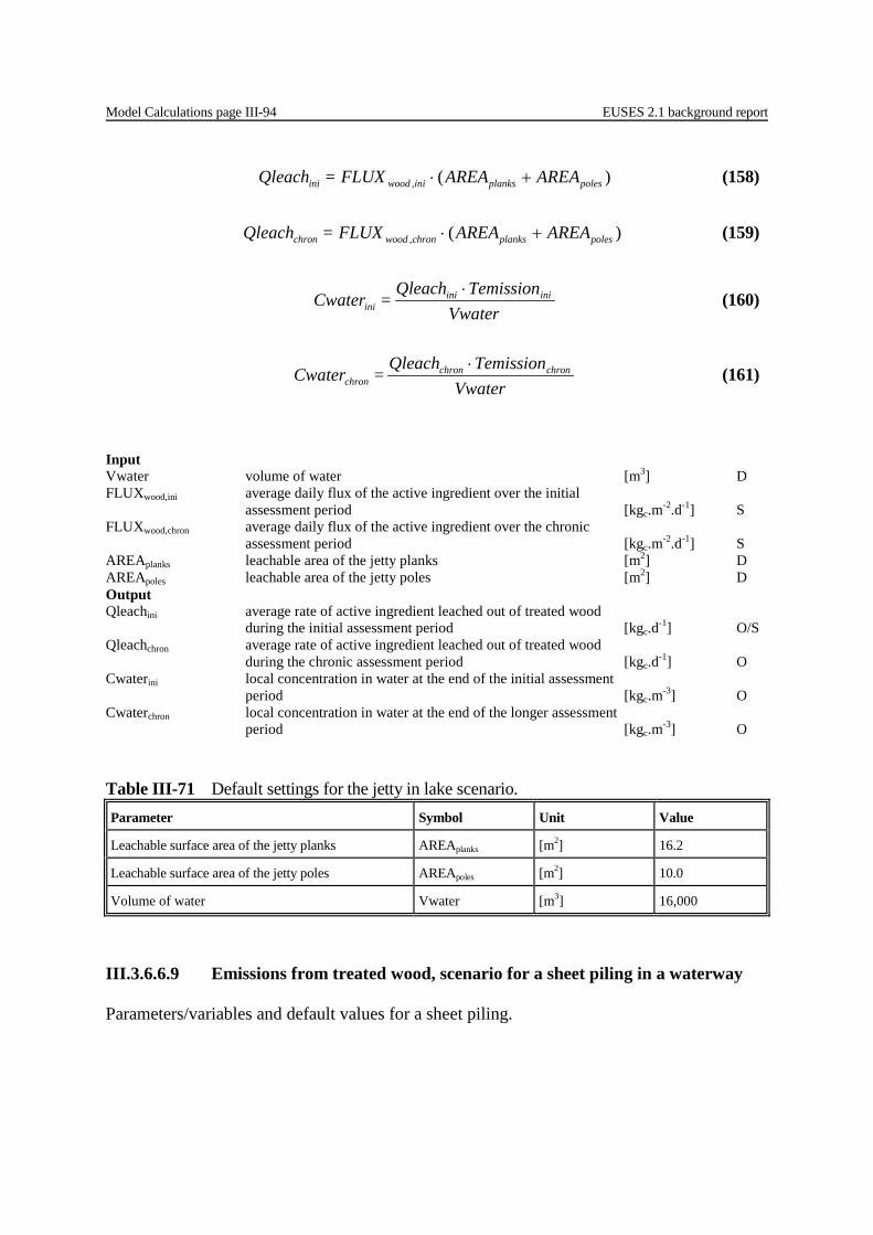
Model Calculations page III-94 EUSES 2.1 background report
Input Vwater volume of water [m3] D FLUXwood,ini average daily flux of the active ingredient over the initial assessment period [kgc.m-2.d-1] S FLUXwood,chron average daily flux of the active ingredient over the chronic assessment period [kgc.m-2.d-1] S AREAplanks leachable area of the jetty planks [m2] D AREApoles leachable area of the jetty poles [m2] D Output Qleachini average rate of active ingredient leached out of treated wood during the initial assessment period [kgc.d-1] O/S Qleachchron average rate of active ingredient leached out of treated wood during the chronic assessment period [kgc.d-1] O Cwaterini local concentration in water at the end of the initial assessment period [kgc.m-3] O Cwaterchron local concentration in water at the end of the longer assessment period [kgc.m-3] O
III.3.6.6.9 Emissions from treated wood, scenario for a sheet piling in a waterway Parameters/variables and default values for a sheet piling.
AREAAREA FLUX= Qleach polesplanksiniwoodini )(, +⋅ (158)
AREAAREA FLUX= Qleach polesplankschronwoodchron )(, +⋅ (159)
Vwater
Temission Qleach = Cwater iniini
ini⋅ (160)
Vwater
Temission Qleach = Cwater chronchron
chron⋅ (161)
Table III-71 Default settings for the jetty in lake scenario. Parameter Symbol Unit Value
Leachable surface area of the jetty planks AREAplanks [m2] 16.2
Leachable surface area of the jetty poles AREApoles [m2] 10.0
Volume of water Vwater [m3] 16,000
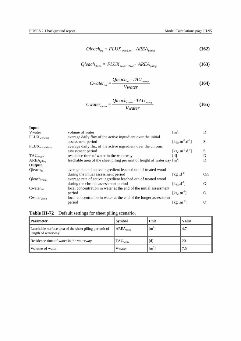
EUSES 2.1 background report Model Calculations page III-95
Input Vwater volume of water [m3] D FLUXwood,ini average daily flux of the active ingredient over the initial assessment period [kgc.m-2.d-1] S FLUXwood,chron average daily flux of the active ingredient over the chronic assessment period [kgc.m-2.d-1] S TAUwway residence time of water in the waterway [d] D AREApiling leachable area of the sheet piling per unit of lenght of waterway [m2] D Output Qleachini average rate of active ingredient leached out of treated wood during the initial assessment period [kgc.d-1] O/S Qleachchron average rate of active ingredient leached out of treated wood during the chronic assessment period [kgc.d-1] O Cwaterini local concentration in water at the end of the initial assessment period [kgc.m-3] O Cwaterchron local concentration in water at the end of the longer assessment period [kgc.m-3] O
pilinginiwoodini AREA FLUX= Qleach ⋅, (162)
AREA FLUX= Qleach pilingchronwoodchron ⋅, (163)
Vwater
TAU Qleach = Cwater wwayini
ini
⋅ (164)
Vwater
TAU Qleach = Cwater wwaychron
chron
⋅ (165)
Table III-72 Default settings for sheet piling scenario. Parameter Symbol Unit Value
Leachable surface area of the sheet piling per unit of length of waterway
AREApiling [m2] 4.7
Residence time of water in the waterway TAUwway [d] 20
Volume of water Vwater [m3] 7.5

Model Calculations page III-96 EUSES 2.1 background report
III.3.6.6.10 Emissions from treated wood, scenario for a wharf in salt water Parameters/variables and default values for a wharf.
A) poles and planks are considered separately
polesiniwatersaltplanksiniwaterini AREA FLUXAREA FLUX= Qleach ⋅+⋅ ,, (166)
AREA FLUXAREA FLUX= Qleach poleschronwatersaltplankschronwaterchron ⋅+⋅ ,, (167)
B) poles and planks are considered together, leaching based on test with de-ionised water
)(, polesplanksiniwaterini AREA AREA FLUX= Qleach +⋅ (168)
)(, AREA AREA FLUX= Qleach polesplankschronwaterchron ⋅+⋅ (169)
A+B) Vwater
TAU Qleach = Cwater wwayini
ini
⋅ (170)
Vwater
TAU Qleach = Cwater wwaychron
chron
⋅ (171)

EUSES 2.1 background report Model Calculations page III-97
Input Vwater volume of water [m3] D FLUXwater,ini average daily flux of the active ingredient over the initial assessment period, based on test with de-ionised water [kgc.m-2.d-1] S FLUXwater,chron average daily flux of the active ingredient over the chronic assessment period, based on test with de-ionised water [kgc.m-2.d-1] S FLUXsalt water,ini average daily flux of the active ingredient over the initial assessment period, based on test with simulated sea water [kgc.m-2.d-1] S FLUXsalt water,chron average daily flux of the active ingredient over the chronic assessment period, based on test with simulated sea water [kgc.m-2.d-1] S TAUseawater residence time of water in the waterway [d] D AREApoles leachable area of the wharf poles [m2] D AREAplanks leachable area of the wharf planks [m2] D Output Qleachini average rate of active ingredient leached out of treated wood during the initial assessment period [kgc.d-1] O Qleachchron average rate of active ingredient leached out of treated wood during the chronic assessment period [kgc.d-1] O Csea waterini local concentration in sea water at the end of the initial assessment period [kgc.m-3] O Csea waterchron local concentration in sea water at the end of the longer assessment period [kgc.m-3] O
Professional and private use, non industrial III.3.6.6.11 Wood preservatives used in indoors curative and preventive treatments, fumigation (professional use only) The model for curative and preventive wood treatment through indoor fumigation, the input for the biocide has to be specified as the amount for a single application.
( ) ( )
1F1 F1QVtreat
= Elocal disinretsubstair
−⋅−⋅⋅ (172)
(the 1 in the formula is one day of the emission episode)
Table III-73 Default settings for the wharf scenario. Parameter Symbol Unit Value
Leachable surface area of the wharf poles AREApoles [m2] 296
Leachable surface area of the wharf planks AREAplanks [m2] 911
Residence time of water in the waterway TAUwway [d] 0.5
Volume of water Vwater [m3] 1000

Model Calculations page III-98 EUSES 2.1 background report
Input Qsubst amount of active ingredient used [kg.m-3] S Vtreat treated volume [m3] S Fret fraction of retention in goods [-] D Fdisin fraction of disintegration [-] D Temissionfogging number of emission days for fogging [d] S Output Elocalair local emission to air during episode [kg.d-1] O Temission number of emission days
Parameters required for distribution modules
Defaults for this scenario Unit Value
Temission Temissionfogging [d] 1
Table III-74 Default settings for calculating releases from indoors applications, fumigation
Parameter Symbol Unit Value
Treated volume
chamber/container
small room (e.g. museum)
big volume (e.g. church)
Vtreat [m3]
100
300
10,000
Fraction of retention in goods Fret [-] 0.02
Fraction of disintegration Fdisin [-] 0.001
III.3.6.6.12 Wood preservatives used in curative and preventive outdoor treatments, brushing Emissions from brushing outdoors for fence, house (only soil) and bridge (only water): brushFsoilRHOprodCprodQprod ⋅⋅⋅⋅itemitemsoil, AREA = Elocal (173)
brushFwaterRHOprodCprodQprod ⋅⋅⋅⋅itemitemwater, AREA = Elocal (174)
RHOsoilVsoil
Elocal = Clocal
item
brushsoil,brushsoil, ⋅
(175)
item
brushwater,brushwater, Vwater
Elocal = Clocal (176)
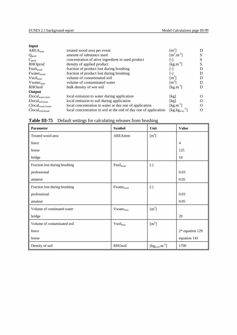
EUSES 2.1 background report Model Calculations page III-99
Input AREAitem treated wood area per event [m2] D Qprod amount of substance used [m3.m-2] S Cprod concentration of ative ingredient in used product [-] S RHOprod density of applied product [kg.m-3] S Fsoilbrush fraction of product lost during brushing [-] D Fwaterbrush fraction of product lost during brushing [-] D Vsoilitem volume of contaminated soil [m3] D Vwateritem volume of contaminated water [m3] D RHOsoil bulk density of wet soil [kg.m-3] D Output Elocalwater,item local emission to water during application [kg] O Elocalsoil,item local emission to soil during application [kg] O Clocalwater,brush local concentration in water at day one of application [kg.m-3] O Clocalsoil,bruah local concentration in soil at the end of day one of application [kg.kgwwt
-1] O Table III-75 Default settings for calculating releases from brushing
Parameter Symbol Unit Value
Treated wood area
fence
house
bridge
AREAitem [m2]
4
125
10
Fraction lost during brushing
professional
amateur
Fsoilbrush [-]
0.03
0.05
Fraction lost during brushing
professional
amateur
Fwaterbrush [-]
0.03
0.05
Volume of contimated water
bridge
Vwateritem [m3]
20
Volume of contaminated soil
fence
house
Vsoilitem [m3]
2* equation 129
equation 143
Density of soil RHOsoil [kgwwt.m-3] 1700
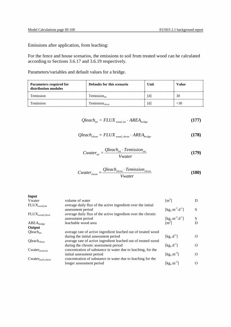
Model Calculations page III-100 EUSES 2.1 background report
Emissions after application, from leaching: For the fence and house scenarios, the emissions to soil from treated wood can be calculated according to Sections 3.6.17 and 3.6.19 respectively. Parameters/variables and default values for a bridge.
Parameters required for distribution modules
Defaults for this scenario Unit Value
Temission Temissionini [d] 30
Temission Temissionchron [d] >30
Input Vwater volume of water [m3] D FLUXwood,ini average daily flux of the active ingredient over the initial assessment period [kgc.m-2.d-1] S FLUXwood,chron average daily flux of the active ingredient over the chronic assessment period [kgc.m-2.d-1] S AREAbridge leachable wood area [m2] D Output Qleachini average rate of active ingredient leached out of treated wood during the initial assessment period [kgc.d-1] O Qleachchron average rate of active ingredient leached out of treated wood during the chronic assessment period [kgc.d-1] O Cwaterleach,ini concentration of substance in water due to leaching, for the initial assessment period [kgc.m-3] O Cwaterleach,chron concentration of substance in water due to leaching for the longer assessment period [kgc.m-3] O
AREA FLUX= Qleach bridgeiniwoodini ⋅, (177)
AREA FLUX= Qleach bridgechronwoodchron ⋅, (178)
Vwater
Temission Qleach = Cwater iniini
ini⋅ (179)
Vwater
Temission Qleach = Cwater chronchron
chron⋅ (180)
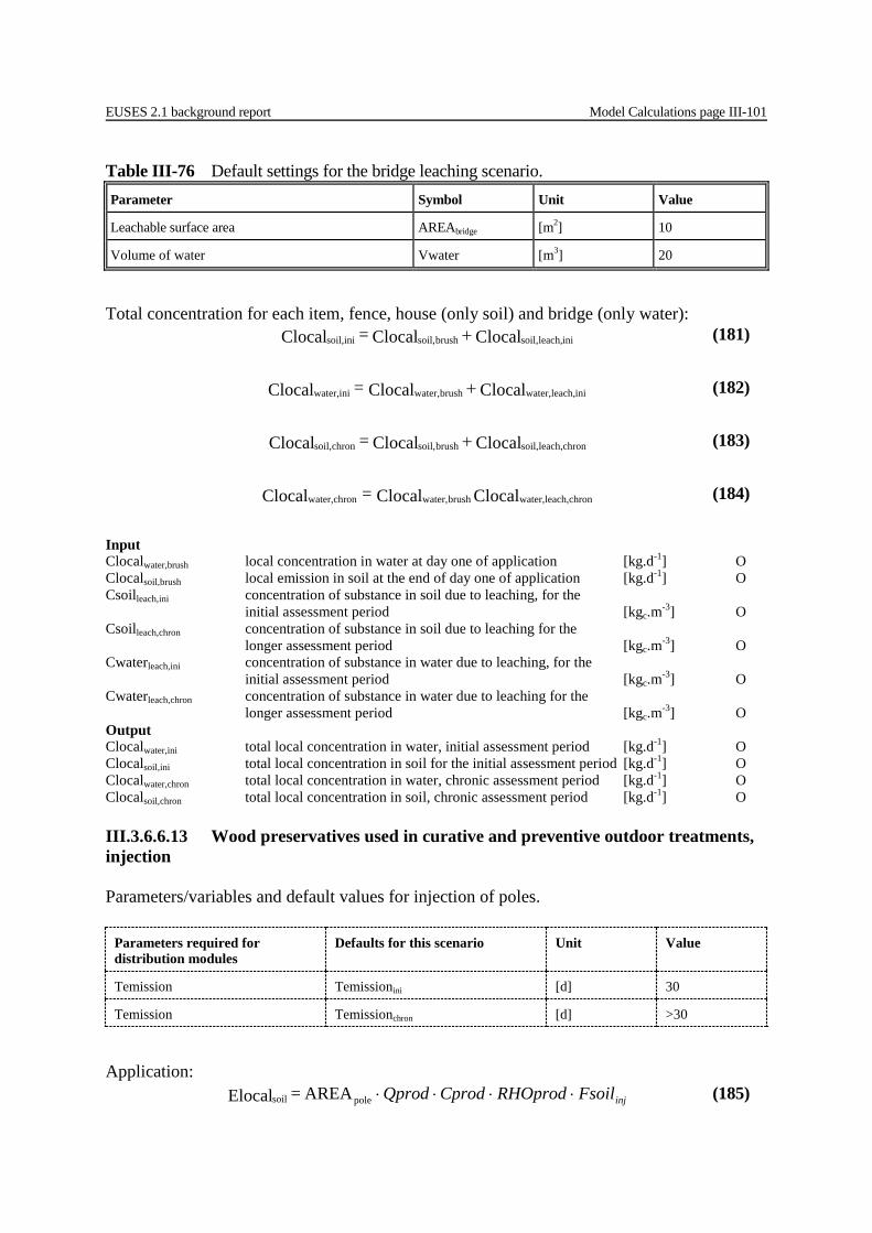
EUSES 2.1 background report Model Calculations page III-101
Total concentration for each item, fence, house (only soil) and bridge (only water): ClocalClocal = Clocal inileach,soil,brushsoil,inisoil, + (181)
ClocalClocal= Clocal inileach,water,brushwater,iniwater, + (182)
ClocalClocal = Clocal chronleach,soil,brushsoil,chronsoil, + (183)
ClocalClocal=Clocal chronleach,water,brushwater,chronwater, (184)
Input Clocalwater,brush local concentration in water at day one of application [kg.d-1] O Clocalsoil,brush local emission in soil at the end of day one of application [kg.d-1] O Csoilleach,ini concentration of substance in soil due to leaching, for the initial assessment period [kgc.m-3] O Csoilleach,chron concentration of substance in soil due to leaching for the longer assessment period [kgc.m-3] O Cwaterleach,ini concentration of substance in water due to leaching, for the initial assessment period [kgc.m-3] O Cwaterleach,chron concentration of substance in water due to leaching for the longer assessment period [kgc.m-3] O Output Clocalwater,ini total local concentration in water, initial assessment period [kg.d-1] O Clocalsoil,ini total local concentration in soil for the initial assessment period [kg.d-1] O Clocalwater,chron total local concentration in water, chronic assessment period [kg.d-1] O Clocalsoil,chron total local concentration in soil, chronic assessment period [kg.d-1] O III.3.6.6.13 Wood preservatives used in curative and preventive outdoor treatments, injection Parameters/variables and default values for injection of poles.
Parameters required for distribution modules
Defaults for this scenario Unit Value
Temission Temissionini [d] 30
Temission Temissionchron [d] >30 Application: injFsoilRHOprodCprodQprod ⋅⋅⋅⋅polesoil AREA = Elocal (185)
Table III-76 Default settings for the bridge leaching scenario. Parameter Symbol Unit Value
Leachable surface area AREAbridge [m2] 10
Volume of water Vwater [m3] 20
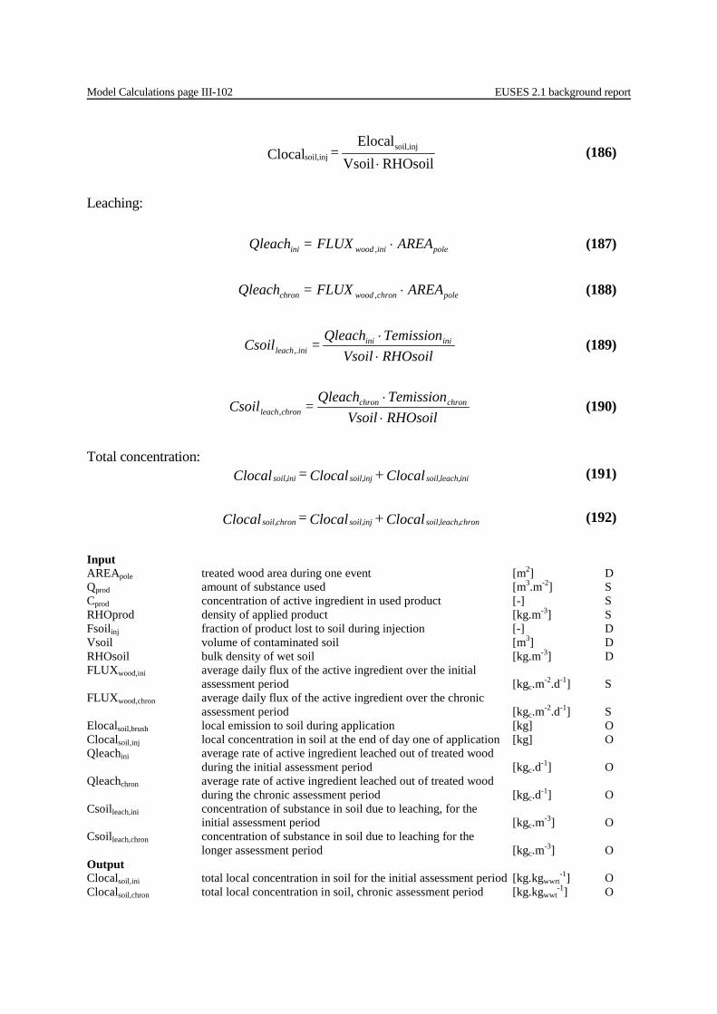
Model Calculations page III-102 EUSES 2.1 background report
RHOsoilVsoil
Elocal = Clocal
injsoil,injsoil, ⋅
(186)
Leaching:
AREA FLUX= Qleach poleiniwoodini ⋅, (187)
AREA FLUX= Qleach polechronwoodchron ⋅, (188)
RHOsoilVsoilTemission Qleach
= Csoil iniiniinileach ⋅
⋅,. (189)
RHOsoilVsoilTemission Qleach
= Csoil chronchronchronleach ⋅
⋅, (190)
Total concentration: ClocalClocal = Clocal inileach,soil,injsoil,inisoil, + (191)
ClocalClocal = Clocal chronleach,soil,injsoil,chronsoil, + (192)
Input AREApole treated wood area during one event [m2] D Qprod amount of substance used [m3.m-2] S Cprod concentration of active ingredient in used product [-] S RHOprod density of applied product [kg.m-3] S Fsoilinj fraction of product lost to soil during injection [-] D Vsoil volume of contaminated soil [m3] D RHOsoil bulk density of wet soil [kg.m-3] D FLUXwood,ini average daily flux of the active ingredient over the initial assessment period [kgc.m-2.d-1] S FLUXwood,chron average daily flux of the active ingredient over the chronic assessment period [kgc.m-2.d-1] S Elocalsoil,brush local emission to soil during application [kg] O Clocalsoil,inj local concentration in soil at the end of day one of application [kg] O Qleachini average rate of active ingredient leached out of treated wood during the initial assessment period [kgc.d-1] O Qleachchron average rate of active ingredient leached out of treated wood during the chronic assessment period [kgc.d-1] O Csoilleach,ini concentration of substance in soil due to leaching, for the initial assessment period [kgc.m-3] O Csoilleach,chron concentration of substance in soil due to leaching for the longer assessment period [kgc.m-3] O Output Clocalsoil,ini total local concentration in soil for the initial assessment period [kg.kgwwrt
-1] O Clocalsoil,chron total local concentration in soil, chronic assessment period [kg.kgwwt
-1] O

EUSES 2.1 background report Model Calculations page III-103
Table III-77 Default settings for calculating releases from injection Parameter Symbol Unit Value
Treated wood area AREApole [m2] 0.8
Fraction lost during brushing Fsoilinj [-] 0.05
Volume of contaminated soil Vsoil [m3] equation 149
Density of soil RHOsoil [kgwwt.m-3] 1700
III.3.6.6.14 Wood preservatives used in curative and preventive outdoor treatments, wrapping Transmission pole: The calculations of the emission to soil are based on the transmission pole scenario and are therefore not repeated here. The same scenario can be used for this special case, with the remark that only the part below soil has to be considered. The treated wood area (below soil) differs for this scenario. It is set at a value of 0.8 m2 by default. This scenario is described in section 3.6.20. Emissions from termite control: airFRHOprodCprodQprod ⋅⋅⋅⋅groundair AREA = Elocal (193)
Based on Qlocalsoil inputs for soil leaching models can be calculated for predictions of the concentration in ground water.
)1(AREA = Qlocal groundsoil airFRHOprodCprodQprod −⋅⋅⋅⋅ (194)
Input AREAground total area treated per day [m2] D Qprod amount of substance used [m3.m-2] S Cprod concentration of active ingredient in used product [-] S Flossair fraction of product emitted to air during application [-] D RHOprod density of the applied product [kg.m-3] S Output Elocalair local emission to air during application [kg.d-1] O Qlocalsoil local quantity applied to soil at day of application [kg.d-1] O

Model Calculations page III-104 EUSES 2.1 background report
Table III-78 Default settings for calculating releases from termite control
Parameter Symbol Unit Value
Total treated area AREAground [m2] 287
Fraction lost to air during application
vapour pressure [Pa] at 20 °C:
< 0.005
0.005-<0.05
0.05-<0.5
0.5-<1.25
1./25-<2.5
>2.5
Flossair [-]
0.001
0.01
0.02
0.075
0.15
0.25
Density of applied product RHOprod [kg.m-3] -
Application rate of used product Qprod [m3.m-2] -
Content of active ingredient in product Cprod [-] -
III.3.6.6.15 Concentrations in soil and water taking removal processes into account Concentrations in soil, taking removal into account: The following scenarios are used to calculate the time dependent concentration in soil. The situation is based on a single emission event during application, followed by leaching from the treated wood during the service life of the treated product, is considered. This corresponds to the scenarios described in sections 3.6.17 to 3.6.28 for professional and domestic use and service life. The following model could be used to calculate the time dependent concentration for this situation. In case for a given product, in-situ treatment is not applicable, i.e. only pre-treated wood in service is considered, the same model can be used by simply not taking emissions during application into account. Parameters/variables and default values for calculating the time weighted concentration.
Parameters required for distribution modules
Defaults for this scenario Unit Value
Temission Temissionini [d] 30
Temission Temissionchron [d] >30
applic
applicsoilapplicsoil Qsoil
Elocal= Clocal ,
, (195)
AREA FLUX= Elocal iteminiwoodinisoil ⋅,, (196)

EUSES 2.1 background report Model Calculations page III-105
AREA FLUX= Elocal itemchronwoodchronsoil ⋅,, (197)
( ) ekQsoil
ElocalClocal
TemissionkkQsoilElocal
= Clocal kTemissioninisoilapplsoil
ini
inisoilinisoil
ini ⋅−−⋅
⋅
−⋅
+⋅
11 ,,
,,
(198)
( ) ekQsoil
ElocalClocal
TemissionkkQsoilElocal
= Clocal kTemissionchronsoilapplsoil
chron
chronsoilchronsoil
chron ⋅−−⋅
⋅
−⋅
+⋅
11 ,,
,,
(199)
K
RHOsoilClocal = Clocal
watersoil
inisoiliniporesoil
−
⋅,,, (200)
K
RHOsoilClocal = Clocal
watersoil
chronsoilchronporesoil
−
⋅,,, (201)
Input Qsoilapplic volume of soil for specific application [m3] O Elocalsoil,applic emission to soil during application, over one day [kg.d-1] O Clocalsoil,appl concentration in soil due to application, for specific scenario [kg.d-1] O Elocalsoil,ini average daily emission to soil due to leaching over initial assessment period, for specific scenario [kg.d-1] O FLUXwood,ini average daily flux of the active ingredient over the initial assessment period [kgc.m-2.d-1] S/O Elocalsoil,chron average daily emission to soil due to leaching over the longer assessment period, for specific scenario [kg.d-1] O FLUXwood,chron average daily flux of the active ingredient over the chronic assessment period [kgc.m-2.d-1] S/O AREAitem leachable wood area for specific item [m2] S/O k first order rate constant for removal from water [-] S Clocalsoil,ini average concentration in soil over initial assessment period, for specific scenario [kg.d-1] O Clocalsoil,chron average concentration in soil over longer assessment period, for specific scenario [kg.d-1] O RHOsoil bulk density of soil [kg.m-3
soil] O Ksoil_water soil-water equilibrium distribution constant [m3
soil.m-3water] Oc
Output Clocalpore,ini average concentration in pore water over initial assessment period, for specific scenario [kg.m-3] O Clocalpore,chron average concentration in pore water over longer assessment period, for specific scenario [kg.m-3] O Concentrations in surface water, static water body and flowing water Two situations can be distinguished: release into a static water body and release into a flowing water body. The first situation corresponds to the scenario for a jetty in a lake (Section 3.6.22). The second situation corresponds to the scenario for a sheet piling (Section

Model Calculations page III-106 EUSES 2.1 background report
3.6.23) as well as for a wharf on the sea (Section 3.6.24). In situ-treatment of wooden structures in permanent contact with water is not very likely and therefore only release due to leaching is taken into account. The following model can be used to take into account removal processes in water bodies. Parameters/variables and default values for calculating the time weighted concentration in water bodies.
Parameters required for distribution modules
Defaults for this scenario Unit Value
Temission Temissionini [d] 30
Temission Temissionchron [d] >30 Static water bodies: AREA FLUX= Elocal iteminiwoodiniwater ⋅,, (202)
AREA FLUX= Elocal itemchronwoodchronwater ⋅,, (203)
Temissionke
kVwaterElocal
= Clocalini
kTemissioniniwater
iniwater
ini
⋅−
−⋅
⋅
⋅−11,, (204)
Temissionke
kVwaterElocal
= Clocalchron
kTemissionchronwater
chronwater
chron
⋅−
−⋅
⋅
⋅−11,, (205)
To take removal from the water column due to adsorption onto suspended matter into account, the concentration should be calculated as follows:
SUSPKpVwaterVsedK
Clocal = Clocal
watersuspwatersed
iniwaterdisswater )1()1( 1
,, ⋅+⋅⋅⋅+ −
−
(206)
SUSPKpVwaterVsedK
Clocal = Clocal
watersuspwatersed
chronwaterdisswater )1()1( 1
,, ⋅+⋅⋅⋅+ −
−
(207)
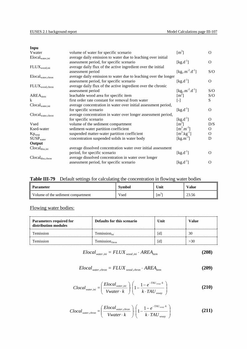
EUSES 2.1 background report Model Calculations page III-107
Inpu Vwater volume of water for specific scenario [m3] O Elocalwater,ini average daily emission to water due to leaching over initial assessment period, for specific scenario [kg.d-1] O FLUXwood,ini average daily flux of the active ingredient over the initial assessment period [kgc.m-2.d-1] S/O Elocalwater,chron average daily emission to water due to leaching over the longer assessment period, for specific scenario [kg.d-1] O FLUXwood,chron average daily flux of the active ingredient over the chronic assessment period [kgc.m-2.d-1] S/O AREAitem leachable wood area for specific item [m2] S/O k first order rate constant for removal from water [-] S Clocalwater,ini average concentration in water over initial assessment period, for specific scenario [kg.d-1] O Clocalwater,chron average concentration in water over longer assessment period, for specific scenario [kg.d-1] O Vsed volume of the sediment compartment [m3] D/S Ksed-water sediment-water partition coefficient [m3.m-3] O Kpsusp suspended matter-water partition coefficient [m3.kg-1] O SUSPwater concentration suspended solids in water body [kg.m-3] D Output Clocaldiss,ini average dissolved concentration water over initial assessment period, for specific scenario [kg.d-1] O Clocaldiss,chron average dissolved concentration in water over longer assessment period, for specific scenario [kg.d-1] O Table III-79 Default settings for calculating the concentration in flowing water bodies
Parameter Symbol Unit Value
Volume of the sediment compartment Vsed [m3] 23.56
Flowing water bodies:
Parameters required for distribution modules
Defaults for this scenario Unit Value
Temission Temissionini [d] 30
Temission Temissionchron [d] >30
AREA FLUX= Elocal iteminiwoodiniwater ⋅,, (208)
AREA FLUX= Elocal itemchronwoodchronwater ⋅,, (209)
TAUke
kVwaterElocal
= Clocalwway
kTAUiniwater
iniwater
wway
⋅−
−⋅
⋅
⋅−11,, (210)
TAUke
kVwaterElocal
= Clocalwway
kTAUchronwater
chronwater
wway
⋅−
−⋅
⋅
⋅−11,, (211)
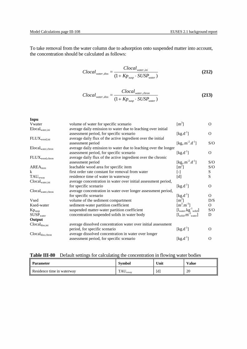
Model Calculations page III-108 EUSES 2.1 background report
To take removal from the water column due to adsorption onto suspended matter into account, the concentration should be calculated as follows:
SUSPKp
Clocal = Clocal
watersusp
iniwaterdisswater )1(
,, ⋅+
(212)
SUSPKp
Clocal = Clocal
watersusp
chronwaterdisswater )1(
,, ⋅+
(213)
Inpu Vwater volume of water for specific scenario [m3] O Elocalwater,ini average daily emission to water due to leaching over initial assessment period, for specific scenario [kg.d-1] O FLUXwood,ini average daily flux of the active ingredient over the initial assessment period [kgc.m-2.d-1] S/O Elocalwater,chron average daily emission to water due to leaching over the longer assessment period, for specific scenario [kg.d-1] O FLUXwood,chron average daily flux of the active ingredient over the chronic assessment period [kgc.m-2.d-1] S/O AREAitem leachable wood area for specific item [m2] S/O k first order rate constant for removal from water [-] S TAUwway residence time of water in waterway [d] S Clocalwater,ini average concentration in water over initial assessment period, for specific scenario [kg.d-1] O Clocalwater,chron average concentration in water over longer assessment period, for specific scenario [kg.d-1] O Vsed volume of the sediment compartment [m3] D/S Ksed-water sediment-water partition coefficient [m3.m-3] O Kpsusp suspended matter-water partition coefficient [lwater.kg-1
solid] S/O SUSPwater concentration suspended solids in water body [lsolid.m-3
water] D Output Clocaldiss,ini average dissolved concentration water over initial assessment period, for specific scenario [kg.d-1] O Clocaldiss,chron average dissolved concentration in water over longer assessment period, for specific scenario [kg.d-1] O Table III-80 Default settings for calculating the concentration in flowing water bodies
Parameter Symbol Unit Value
Residence time in waterway TAUwway [d] 20
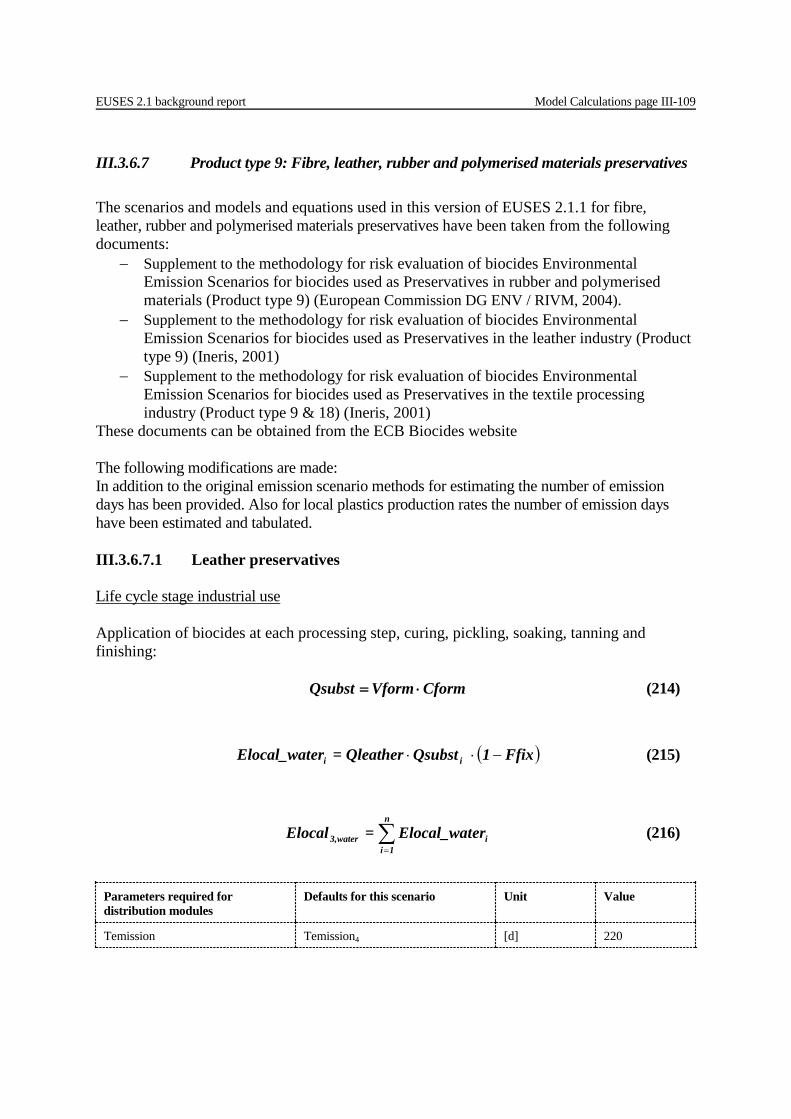
EUSES 2.1 background report Model Calculations page III-109
III.3.6.7 Product type 9: Fibre, leather, rubber and polymerised materials preservatives The scenarios and models and equations used in this version of EUSES 2.1.1 for fibre, leather, rubber and polymerised materials preservatives have been taken from the following documents:
− Supplement to the methodology for risk evaluation of biocides Environmental Emission Scenarios for biocides used as Preservatives in rubber and polymerised materials (Product type 9) (European Commission DG ENV / RIVM, 2004).
− Supplement to the methodology for risk evaluation of biocides Environmental Emission Scenarios for biocides used as Preservatives in the leather industry (Product type 9) (Ineris, 2001)
− Supplement to the methodology for risk evaluation of biocides Environmental Emission Scenarios for biocides used as Preservatives in the textile processing industry (Product type 9 & 18) (Ineris, 2001)
These documents can be obtained from the ECB Biocides website The following modifications are made: In addition to the original emission scenario methods for estimating the number of emission days has been provided. Also for local plastics production rates the number of emission days have been estimated and tabulated. III.3.6.7.1 Leather preservatives Life cycle stage industrial use Application of biocides at each processing step, curing, pickling, soaking, tanning and finishing: CformVformQsubst ⋅= (214)
( )Ffix1 Qsubst Qleather=erElocal_wat ii −⋅⋅ (215)
∑=
n
1iiwater3, erElocal_wat=Elocal (216)
Parameters required for distribution modules
Defaults for this scenario Unit Value
Temission Temission4 [d] 220
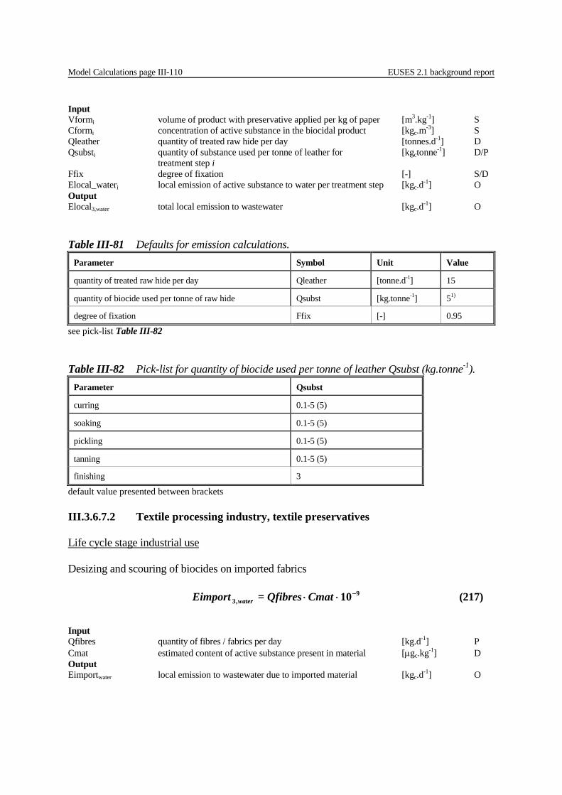
Model Calculations page III-110 EUSES 2.1 background report
Input Vformi volume of product with preservative applied per kg of paper [m3.kg-1] S Cformi concentration of active substance in the biocidal product [kgc.m-3] S Qleather quantity of treated raw hide per day [tonnes.d-1] D Qsubsti quantity of substance used per tonne of leather for [kgctonne-1] D/P treatment step i Ffix degree of fixation [-] S/D Elocal_wateri local emission of active substance to water per treatment step [kgc.d-1] O Output Elocal3,water total local emission to wastewater [kgc.d-1] O Table III-81 Defaults for emission calculations.
Parameter Symbol Unit Value
quantity of treated raw hide per day Qleather [tonne.d-1] 15
quantity of biocide used per tonne of raw hide Qsubst [kg.tonne-1] 51)
degree of fixation Ffix [-] 0.95
see pick-list Table III-82 Table III-82 Pick-list for quantity of biocide used per tonne of leather Qsubst (kg.tonne-1).
Parameter Qsubst
curring 0.1-5 (5)
soaking 0.1-5 (5)
pickling 0.1-5 (5)
tanning 0.1-5 (5)
finishing 3
default value presented between brackets III.3.6.7.2 Textile processing industry, textile preservatives Life cycle stage industrial use Desizing and scouring of biocides on imported fabrics 9
,3 10−⋅⋅Cmat Qfibres=Eimport water (217)
Input Qfibres quantity of fibres / fabrics per day [kg.d-1] P Cmat estimated content of active substance present in material [mgc.kg-1] D Output Eimportwater local emission to wastewater due to imported material [kgc.d-1] O

EUSES 2.1 background report Model Calculations page III-111
Table III-83 Defaults for emission calculations. Parameter Symbol Unit Value
quantity of fibres / fabric treated per day
cotton spinning
wool preparation
wool spinning
silk, synthetic
sewing knit
cotton weaving
wool weaving
silk weaving
others weaving
textile ennobling
house and furnish fabric
other textile goods
cords, filets
non woven
mail fabrics
Qfibres [kg.d-1]
7 000
1 000
2 500
1 000
4 000
2 000
1 000
100
1 500
7 000
500
200
3 000
4 000
2 000
estimated concentration of active substance present in textile material
Default
Wool
Default
DDE
PCB-28/31
heptachlor
Cotton
Default
DDE
DDD
DDT
heptachlor
Cmat [mg.kg-1]
10
0.38
0.07-0.38
0.15-0.34
0.03-0.12
12.4
0.85-4.5
0.09-12.8
0-12.4
0.13-0.45
Life cycle stage industrial use Application of biocides at each textile processing step (i), desizing / scouring, dyeing and finishing (total emissions including emissions due to imported material):

Model Calculations page III-112 EUSES 2.1 background report
( )Ffix1 Qsubst Qfabric=erElocal_wat ii −⋅⋅ (218)
water
n
iiwater EimportwaterElocal=Elocal +∑
=1,3 _ (219)
Parameters required for distribution modules
Defaults for this scenario Unit Value
Temission Temission4 [d] 225
Input Qfabric quantity of treated fabric per day [tonnes.d-1] D Qsubsti quantity of substance used per tonne of fibres/fabric for [kgctonne-1] S treatment step i Ffix degree of fixation [-] S Elocal_wateri local emission of active substance to water per treatment step [kgc.d-1] O Eimportwater local emission to wastewater due to imported material [kgc.d-1] O Output Elocal3,water total local emission to wastewater [kgc.d-1] O Table III-84 Defaults for emission calculations. The highest value is chosen for the worst case
situation. Parameter Symbol Unit Value
quantity of treated fabric per day Qfabric [tonne.d-1] 1)
quantity of substance used per tonne of fabric
permethrin
sulcofuron
permethrin/hexahydropyrimidine
Qsubst [kg.tonne-1] 10
0.35-1.81
8-9.7
0.55-0.825
degree of fixation Ffix [-] 0.7 1) see Table III-83 2) as a worst case, a default value of 10 kg per tonne can be used if no further data is available
Life cycle stage Service life
( )
1
5
1,5,5
,5,
1_−
=∑ −⋅⋅⋅
yTservice
yjkwaterreg
waterk Temission
FtotQsubstFFprodvol=RELEASEreg
k
(220)
∑=
⋅m
kwaterkwater RELEASEreg=RELEASEreg
1,5,
3,5 10 (221)
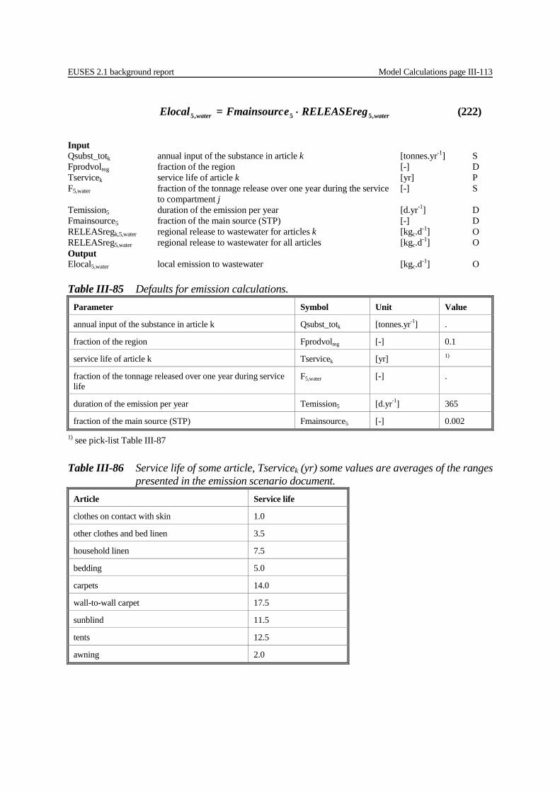
EUSES 2.1 background report Model Calculations page III-113
waterwater RELEASEregeFmainsourc=Elocal ,55,5 ⋅ (222)
Input Qsubst_totk annual input of the substance in article k [tonnes.yr-1] S Fprodvolreg fraction of the region [-] D Tservicek service life of article k [yr] P F5,water fraction of the tonnage release over one year during the service [-] S to compartment j Temission5 duration of the emission per year [d.yr-1] D Fmainsource5 fraction of the main source (STP) [-] D RELEASregk,5,water regional release to wastewater for articles k [kgc.d-1] O RELEASreg5,water regional release to wastewater for all articles [kgc.d-1] O Output Elocal5,water local emission to wastewater [kgc.d-1] O Table III-85 Defaults for emission calculations.
Parameter Symbol Unit Value
annual input of the substance in article k Qsubst_totk [tonnes.yr-1] .
fraction of the region Fprodvolreg [-] 0.1
service life of article k Tservicek [yr] 1)
fraction of the tonnage released over one year during service life
F5,water [-] .
duration of the emission per year Temission5 [d.yr-1] 365
fraction of the main source (STP) Fmainsource5 [-] 0.002
1) see pick-list Table III-87 Table III-86 Service life of some article, Tservicek (yr) some values are averages of the ranges
presented in the emission scenario document. Article Service life
clothes on contact with skin 1.0
other clothes and bed linen 3.5
household linen 7.5
bedding 5.0
carpets 14.0
wall-to-wall carpet 17.5
sunblind 11.5
tents 12.5
awning 2.0
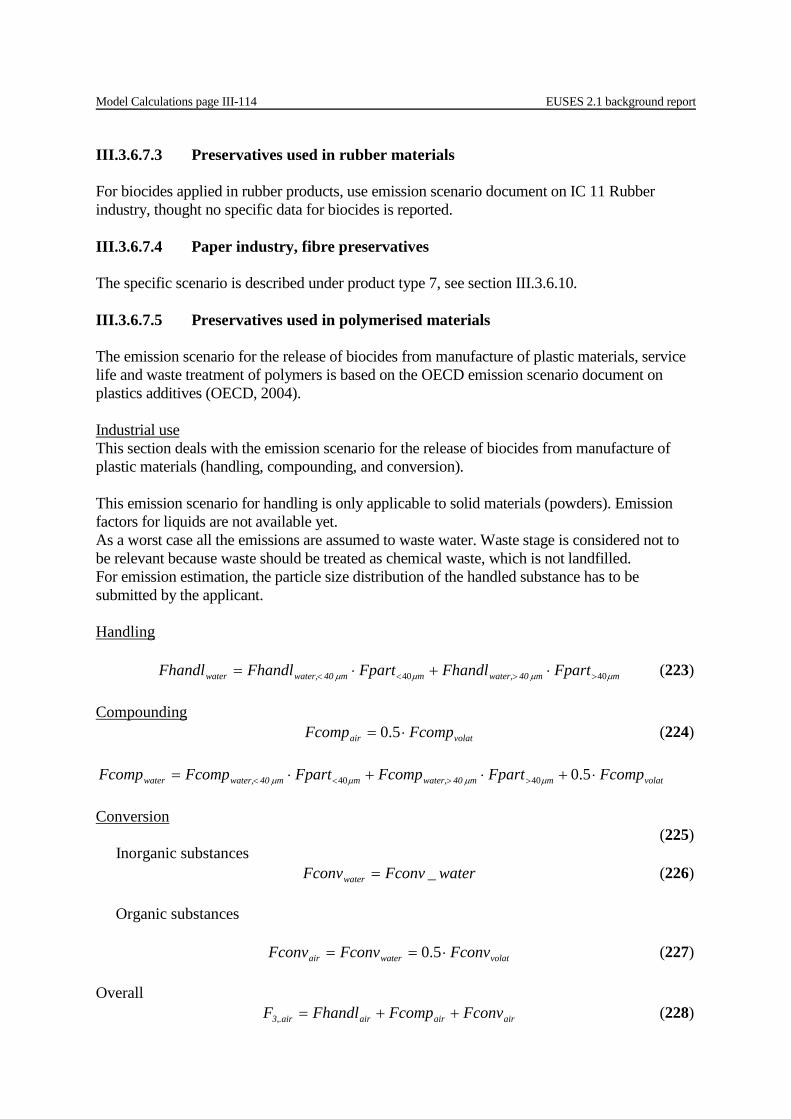
Model Calculations page III-114 EUSES 2.1 background report
III.3.6.7.3 Preservatives used in rubber materials For biocides applied in rubber products, use emission scenario document on IC 11 Rubber industry, thought no specific data for biocides is reported. III.3.6.7.4 Paper industry, fibre preservatives The specific scenario is described under product type 7, see section III.3.6.10. III.3.6.7.5 Preservatives used in polymerised materials The emission scenario for the release of biocides from manufacture of plastic materials, service life and waste treatment of polymers is based on the OECD emission scenario document on plastics additives (OECD, 2004). Industrial use This section deals with the emission scenario for the release of biocides from manufacture of plastic materials (handling, compounding, and conversion). This emission scenario for handling is only applicable to solid materials (powders). Emission factors for liquids are not available yet. As a worst case all the emissions are assumed to waste water. Waste stage is considered not to be relevant because waste should be treated as chemical waste, which is not landfilled. For emission estimation, the particle size distribution of the handled substance has to be submitted by the applicant. Handling mm 40 water,mm 40 water,water FpartFhandlFpartFhandlFhandl mmmm 4040 >><< ⋅+⋅= (223) Compounding volatair FcompFcomp ⋅= 5.0 (224)
volatmm 40 water,mm 40 water,water FcompFpartFcompFpartFcompFcomp ⋅+⋅+⋅= >><< 5.04040 mmmm Conversion (225) Inorganic substances waterFconvFconvwater _= (226) Organic substances volatwaterair FconvFconvFconv ⋅== 5.0 (227) Overall airairair3,.air FconvFcompFhandlF ++= (228)
EUSES 2.1 background report Model Calculations page III-115
waterwaterwater3,.water FconvFcompFhandlF ++= (229) The emission scenario does not provide the number of emission days. To establish the number of emission days and size of a point source for emission estimation at the local scale table B3.9 for industrial category 11, of Appendix I of the Technical Guidance Document (EC, 2003) should be used to calculate the number of emission days (Temission). The regional tonnage, TONNAGEreg, should be corrected for the estimation of the fraction of the main source and the number of emission days by the concentration or fraction of the substance in the polymer (Fpolymer). This yields the tonnage of the polymer in the EU. The concentration in the polymer has to be supplied by the notifier. The fraction of the tonnage for the region is by default 0.1 for existing substance with wide spread use. For new substances with limited use the fraction of the tonnage for the region is by default 1, according to the TGD (EC, 2003). TONNAGEgFprodvolreTONNAGEreg ⋅= (230) FpolymerTONNAGEregTONNAGEreg polymer = (231)
3
365Temission
FeFmainsourcTONNAGEregElocal air3,3air3, ⋅⋅⋅= (232)
3
365Temission
FeFmainsourcTONNAGEregElocal water3,3water3, ⋅⋅⋅= (233)
Alternatively local production rates (Qplastic) for different types of polymers and for each processing type can be used (Table III-91). The production rates provided in the emission scenario specifically refer to the situation in the United Kingdom. Therefore using these data should be done with care as the distribution of size of companies may differ might differ from one country to another. Using the local production rates the number of working days can be estimated from the information provided in Table B3.9 from the TGD. The number of working days is listed in Table III-92). /NwdaysFFpolymerQplasticElocal air3,air3, ⋅⋅= (234) /NwdaysFFpolymerQplasticElocal water3,water3, ⋅⋅= (235)
Model Calculations page III-116 EUSES 2.1 background report
Input - processing system [-] P - polymer type [-] P - type of substance [-] P - type of conversion process [-] P - type of product [-] P VOLATILITY volatility of the substance [High/medium/low]S WATERRINSE Is water used for cleaning operations? [yes/no] P Fpart<40 μm particle size fraction < 40 um [-] S Fpart>40 μm particle size fraction > 40 um [-] S Fhandlwater,<40 μm fraction released to water for particle size fraction < 40 μm [-] D Fhandlwater,>40 μm fraction released to water for particle size fraction > 40 μm [-] D Fhandlair,<40 μm fraction released to air for particle size fraction < 40 μm [-] D Fhandlair,>40 μm fraction released to air for particle size fraction > 40 μm [-] D Fcompwater,<40 μm fraction released to water for particle size fraction < 40 μm [-] S Fcompwater,>40 μm fraction released to water for particle size fraction > 40 μm [-] S Fhandlair fraction released to air during materials handling [-] Oc
Fhandlwater fraction released to water during materials handling [-] Oc
Fcompvolat fraction released at compounding, which is related to the volatility of the substance used [-] D Fcompair fraction release to air during compounding [kg.kg-1] Oc
Fcompwater fraction release to water during compounding [kg.kg-1] Oc
Fconvvolat fraction released at conversion, which is related to the volatility of the substance used [-] D Fcompair fraction release to air during compounding [kg.kg-1] Oc
Fcompwater fraction release to water during compounding [kg.kg-1] Oc
F3,air emission factor to air for processing [-] O F3,water emission factor to (waste)water for processing [-] O TONNAGE relevant tonnage of the substance in EU for this application [kg.d-1] S TONNAGEreg relevant tonnage the substance in the region for this application [kg.d-1] S/O Fpolymer fraction of active substance in the in the plastic material [kg.kg-1] S Fprodvolreg fraction for the region [-] D TONNAGEregpolymer amount of plastic produced with the substance in the region [kg.d-1] O Fmainsource3 fraction of the main source for polymer processing [-] D Temission3 number of emission days [d] O Nwdays number of working days at the local source [d.yr-1] D/O Qplastic local production rate for specific type of plastic and process [kg.yr-1] D/O Output Elocal3,water local emission of active substance to waste water [kgc.d-1] O Elocal3,air local emission of active substance to waste water [kgc.d-1] O
EUSES 2.1 background report Model Calculations page III-117
Table III-87 Default settings for calculating releases of biocides used as preservatives in the
polymers industry Parameter Symbol Unit Value
Quantity of plastic produced Qplastic [kg.d-1] Table III-91
Fraction released to water during materials handling
WATERRINSE = no
WATERRINSE = yes
particle size < 40 um
particle size > 40 um
Fhandlingwater [-]
n.a.*
0.006
0.002
Fraction volatilised during compounding**
Volatility at: 20 C° 150 C°:
high > 1.10-4 Pa > 50 Pa
medium 1.10-4 – 1.10-5 Pa 5-50 Pa
low < 1.10-5 Pa < 5 Pa
Fcompvolat [-]
0.0005
0.0001
0.00002
Fraction released to water during compounding
WATERRINSE = no
WATERRINSE = yes
particle size < 40 um
particle size > 40 um
Fcompwater [-]
n.a.*
0.0005
0.0001
Fraction released to water during conversion
Inorganic substances
Conversion process
- grinding/machining
- other processes
Organic substance
Fconv_water [-]
0.025
0.0001
n.a.
Fraction of substance volatilised during conversion
Inorganic substances
Organic substance
Fconvvolat [-]
n.a.
Table III-88
n.a.: not applicable. * Waste generated from the processing stages is considered not applicable because it should be treated as chemical waste and as such not be released at landfills. ** if processing temperature (compounding or conversion) is exceeding 200 °C then emission factor should by a factor of ten higher
Model Calculations page III-118 EUSES 2.1 background report
Table III-88 Default emission factors, Fconvvolat (-) for different conversion processes and
types of articles produced based on the vapour pressure (Pa) at 150 C° of the applied substance. High (> 50 Pa), medium (5 - 50 Pa) and low (<5 Pa) vapour pressure.
Type of Process Type of product Vapour pressure Value*
Open solid
foamed
high
medium
low
high
medium
low
0.0025
0.0005
0.0001
0.005
0.001
0.0002
Partially open All high
medium
low
0.0015
0.0003
0.00006
Closed All high
medium
low
0.0005
0.0001
0.00002
* if processing temperature (compounding or conversion) is exceeding 200 °C then emission factor should by a factor of ten higher Table III-89 Default settings for calculating concentrations in the STP or surface water and air
of compounds used in polymers Parameter Symbol Unit Value
Fraction for the region Fprodvolreg [-] 0.1
Table III-90 Fraction of the main source, Fmainsource3 [-], and the number of emission days,
Temission3 [d], for the processing stage of polymers and polymers with preservatives based on the corrected regional tonnage, TONNAGEregpolymer [tonnes .yr-1], of the biocide
TONNAGEregpolymer Fmainsource3 Temission3
< 10
≥10-<50
≥50-<500
≥500-<5,000
≥5,000-<25,000
≥ 25,000
0,5
0,35
0.25
0.15
0.10
0.05
2 ⋅ Fmainsource ⋅ TONNAGEreg
Fmainsource ⋅ TONNAGEreg
0.4 ⋅ Fmainsource ⋅ TONNAGEreg
0.4 ⋅ Fmainsource ⋅ TONNAGEreg
300
300
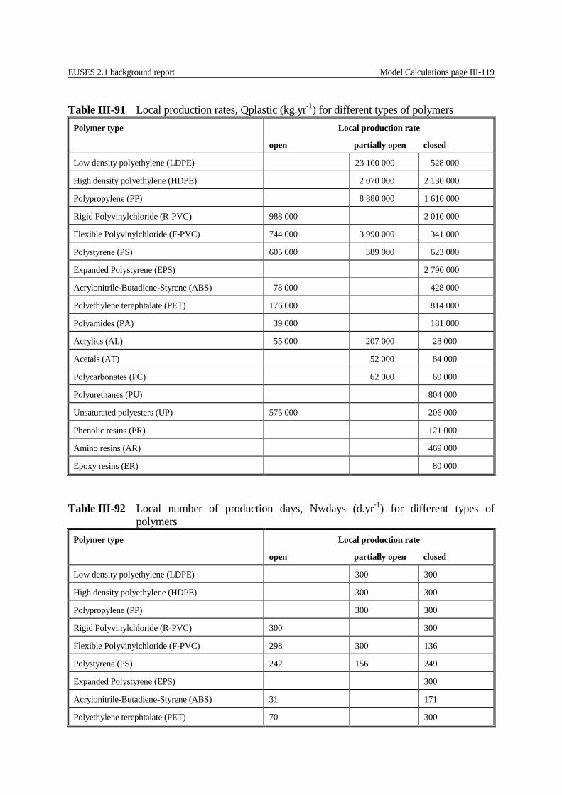
EUSES 2.1 background report Model Calculations page III-119
Table III-91 Local production rates, Qplastic (kg.yr-1) for different types of polymers Polymer type Local production rate
open partially open closed
Low density polyethylene (LDPE) 23 100 000 528 000
High density polyethylene (HDPE) 2 070 000 2 130 000
Polypropylene (PP) 8 880 000 1 610 000
Rigid Polyvinylchloride (R-PVC) 988 000 2 010 000
Flexible Polyvinylchloride (F-PVC) 744 000 3 990 000 341 000
Polystyrene (PS) 605 000 389 000 623 000
Expanded Polystyrene (EPS) 2 790 000
Acrylonitrile-Butadiene-Styrene (ABS) 78 000 428 000
Polyethylene terephtalate (PET) 176 000 814 000
Polyamides (PA) 39 000 181 000
Acrylics (AL) 55 000 207 000 28 000
Acetals (AT) 52 000 84 000
Polycarbonates (PC) 62 000 69 000
Polyurethanes (PU) 804 000
Unsaturated polyesters (UP) 575 000 206 000
Phenolic resins (PR) 121 000
Amino resins (AR) 469 000
Epoxy resins (ER) 80 000
Table III-92 Local number of production days, Nwdays (d.yr-1) for different types of
polymers Polymer type Local production rate
open partially open closed
Low density polyethylene (LDPE) 300 300
High density polyethylene (HDPE) 300 300
Polypropylene (PP) 300 300
Rigid Polyvinylchloride (R-PVC) 300 300
Flexible Polyvinylchloride (F-PVC) 298 300 136
Polystyrene (PS) 242 156 249
Expanded Polystyrene (EPS) 300
Acrylonitrile-Butadiene-Styrene (ABS) 31 171
Polyethylene terephtalate (PET) 70 300
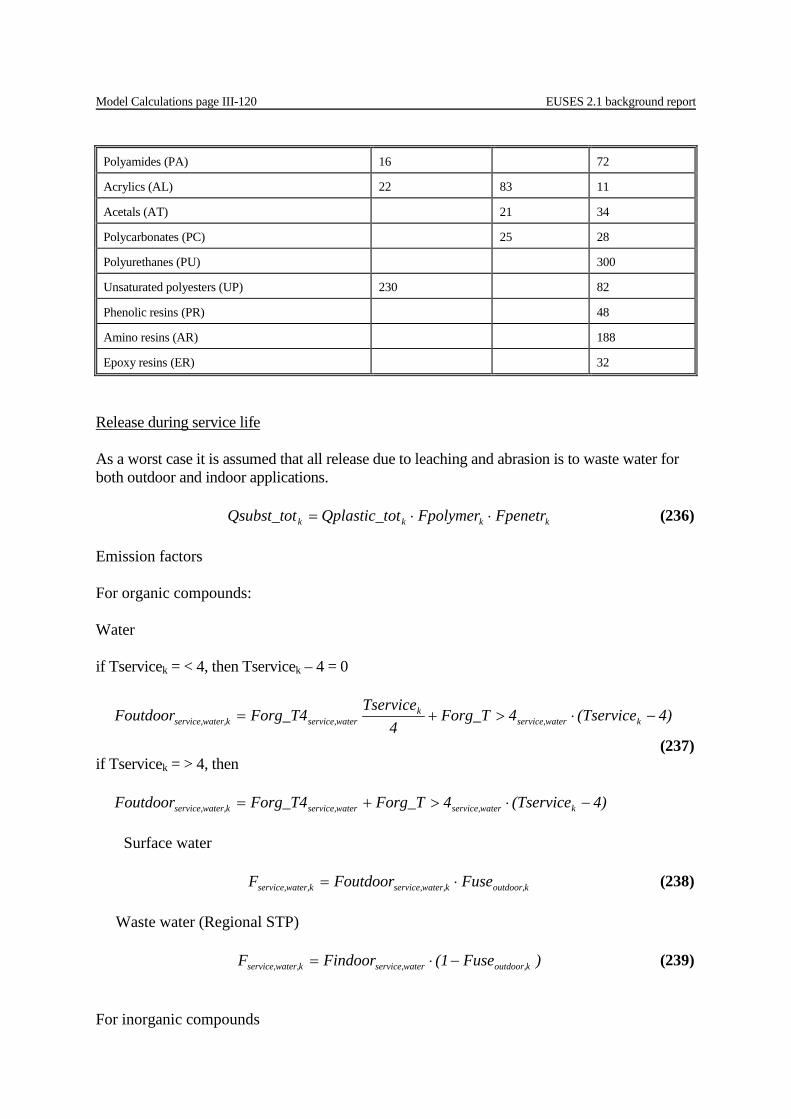
Model Calculations page III-120 EUSES 2.1 background report
Polyamides (PA) 16 72
Acrylics (AL) 22 83 11
Acetals (AT) 21 34
Polycarbonates (PC) 25 28
Polyurethanes (PU) 300
Unsaturated polyesters (UP) 230 82
Phenolic resins (PR) 48
Amino resins (AR) 188
Epoxy resins (ER) 32
Release during service life As a worst case it is assumed that all release due to leaching and abrasion is to waste water for both outdoor and indoor applications. kkkk FpenetrFpolymerotQplastic_tQsubst_tot ⋅⋅= (236) Emission factors For organic compounds: Water if Tservicek = < 4, then Tservicek – 4 = 0
4)(Tservice4Forg_T4
TserviceForg_T4Foutdoor kwaterservice,
kwaterservice,kwater,service, −⋅>+=
(237) if Tservicek = > 4, then 4)(Tservice4Forg_TForg_T4Foutdoor kwaterservice,waterservice,kwater,service, −⋅>+= Surface water koutdoor,kwater,service,kwater,service, FuseFoutdoorF ⋅= (238) Waste water (Regional STP) )Fuse(1FindoorF koutdoor,waterservice,kwater,service, −⋅= (239) For inorganic compounds
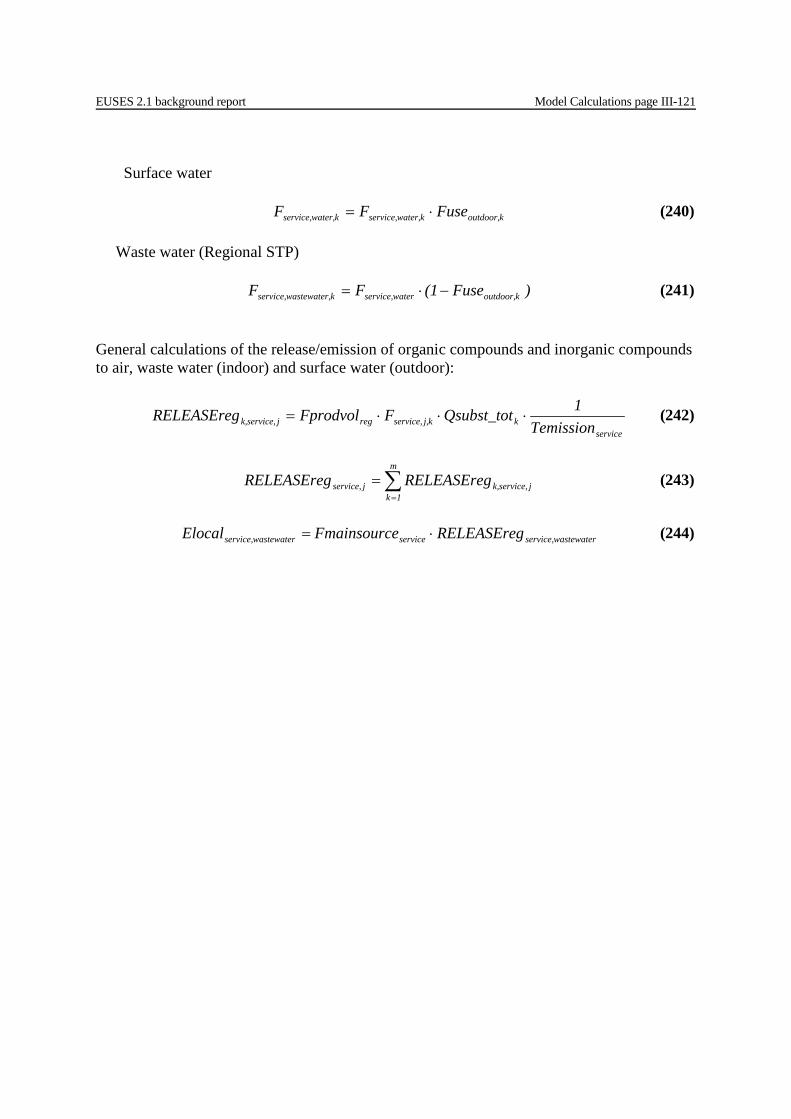
EUSES 2.1 background report Model Calculations page III-121
Surface water koutdoor,kwater,service,kwater,service, FuseFF ⋅= (240) Waste water (Regional STP) )Fuse(1FF koutdoor,waterservice,k,wastewaterservice, −⋅= (241) General calculations of the release/emission of organic compounds and inorganic compounds to air, waste water (indoor) and surface water (outdoor):
service
kkj,service,regjservice,k, Temission1Qsubst_totFFprodvolRELEASEreg ⋅⋅⋅= (242)
∑=
=m
1kjservice,k,jservice, RELEASEregRELEASEreg (243)
wastewaterservice,servicewastewaterservice, RELEASEregeFmainsourc Elocal ⋅= (244)
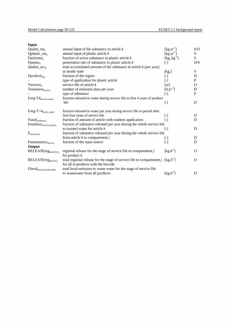
Model Calculations page III-122 EUSES 2.1 background report
Input Qsubst_totk annual input of the substance in article k [kg.yr-1] S/O Qplastic_totk annual input of plastic article k [kg.yr-1] S Fpolymerk fraction of active substance in plastic article k [kgc.kg-1] S Fpenetrk penetration rate of substance in plastic article k [-] D/S Qsubst_acck total accumulated amount of the substance in article k (per year) at steady state [kgc] S Fprodvolreg fraction of the region [-] D - type of application for plastic article [-] P Tservicek service life of article k [yr] O Temissionservice number of emission days per year [d.yr-1] D - type of substance [-] P Forg-T4service,water fraction released to water during service life in first 4 years of product life [-] D Forg-T>4servic,water fraction released to water per year during service life in period after first four years of service life [-] D Fusedoutdoor,k fraction of amount of article with outdoor application [-] D Foutdoorservice,water,k fraction of substance released per year during the whole service life to (waste) water for article k [-] D Fservice,j,k fraction of substance released per year during the whole service life from article k to compartment j [-] D Fmainsourceservice fraction of the main source [-] D Output RELEASEregk,service,j regional release for the stage of service life to compartment j [kg.d-1] O for product k RELEASEregservice,j total regional release for the stage of service life to compartment j [kg.d-1] O for all m products with the biocide Elocalservice,wastewater total local emission to waste water for the stage of service life to wastewater from all products [kg.d-1] O
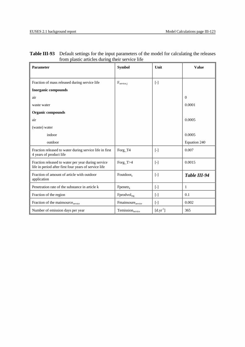
EUSES 2.1 background report Model Calculations page III-123
Table III-93 Default settings for the input parameters of the model for calculating the releases
from plastic articles during their service life Parameter Symbol Unit Value
Fraction of mass released during service life
Inorganic compounds
air
waste water
Organic compounds
air
(waste) water
indoor
outdoor
Fservice,j [-]
0
0.0001
0.0005
0.0005
Equation 240
Fraction released to water during service life in first 4 years of product life
Forg_T4 [-] 0.007
Fraction released to water per year during service life in period after first four years of service life
Forg_T>4 [-] 0.0015
Fraction of amount of article with outdoor application
Foutdoork [-] Table III-94
Penetration rate of the substance in article k Fpenetrk [-] 1
Fraction of the region Fprodvolreg [-] 0.1
Fraction of the mainsourceservice Fmainsoureservice [-] 0.002
Number of emission days per year Temissionservice [d.yr-1] 365
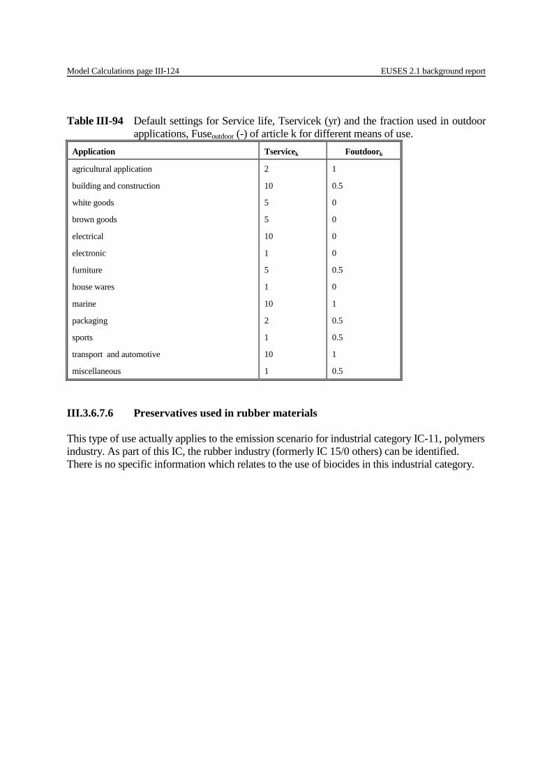
Model Calculations page III-124 EUSES 2.1 background report
Table III-94 Default settings for Service life, Tservicek (yr) and the fraction used in outdoor
applications, Fuseoutdoor (-) of article k for different means of use. Application Tservicek Foutdoork
agricultural application
building and construction
white goods
brown goods
electrical
electronic
furniture
house wares
marine
packaging
sports
transport and automotive
miscellaneous
2
10
5
5
10
1
5
1
10
2
1
10
1
1
0.5
0
0
0
0
0.5
0
1
0.5
0.5
1
0.5
III.3.6.7.6 Preservatives used in rubber materials This type of use actually applies to the emission scenario for industrial category IC-11, polymers industry. As part of this IC, the rubber industry (formerly IC 15/0 others) can be identified. There is no specific information which relates to the use of biocides in this industrial category.
EUSES 2.1 background report Model Calculations page III-125
III.3.6.8 Product type 10: Masonry preservatives The scenarios and models and calculation formulations used in this version of EUSES 2.1.1 for masonry preservatives have been taken from the following documents:
− Supplement to the methodology for risk evaluation of biocides Environmental Emission Scenarios for biocides used as masonry preservatives (Product type 10) (Ineris, 2002)
This document can be obtained from the ECB Biocides website Industrial use Industrial sites There is usually no treatment at industrial sites. Generally biocides are not use at the production of cement, extraction and processing of clay or added to concrete. It is assumed that neither biocides are used to treat products after production and before being marketed. Private and professional use In situ treatment of buildings (preventive and curative) Surfaces made of building materials such as roofs, walls, façades, paths, terraces, etc. can be affected by the development of mosses, lichen, and algae. Biocides can be used to protect and/ or cure building materials. III.3.6.8.1 Masonry preservatives used at situ treatment, spraying Parameters/variables and default values for a roof treated through spraying.

Model Calculations page III-126 EUSES 2.1 background report
Parameters required for distribution modules
Defaults for this scenario Unit Value
Temission Temissionspary [d] 1
Countryside
if GUTTER = no, then
FdriftRHOformFformVform AREAroof = soilElocal roofdriftspray ⋅⋅⋅⋅−_ , (245)
FrunoffRHOformFformVform AREAroof = soilElocal roofrunoff, ⋅⋅⋅⋅_ (246)
RHOsoiladjacentVsoil
soilElocal = adjacentCsoil roofrunoff
roof ⋅__
_ , (247)
RHOsoildistantsoilV
soilElocal = distantsoilC roofdriftspray
roof ⋅−
__
_ , (248)
if GUTTER = yes, then
spray
roof TemissionFrunoffRHOformFformVform AREAroof = waterElocal ⋅⋅⋅⋅_ (249)
RHOsoildistantsoilV
soilElocal = distantsoilC roofdriftspray
roof ⋅−
__
_ , (250)
City
sprayroof Temission
FdriftFrunoffRHOformFformVform AREAroof = waterElocal )(_ +⋅⋅⋅⋅ (251)
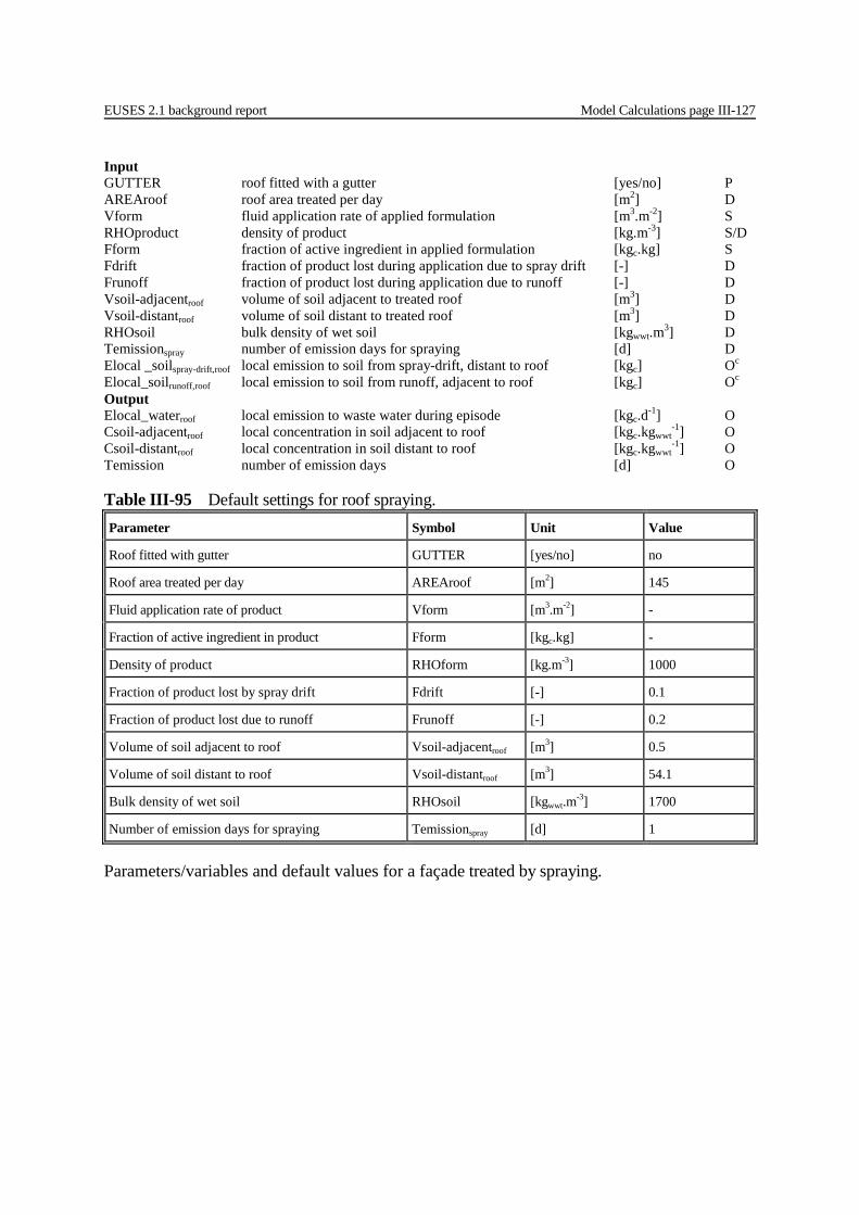
EUSES 2.1 background report Model Calculations page III-127
Input GUTTER roof fitted with a gutter [yes/no] P AREAroof roof area treated per day [m2] D Vform fluid application rate of applied formulation [m3.m-2] S RHOproduct density of product [kg.m-3] S/D Fform fraction of active ingredient in applied formulation [kgc.kg] S Fdrift fraction of product lost during application due to spray drift [-] D Frunoff fraction of product lost during application due to runoff [-] D Vsoil-adjacentroof volume of soil adjacent to treated roof [m3] D Vsoil-distantroof volume of soil distant to treated roof [m3] D RHOsoil bulk density of wet soil [kgwwt.m3] D Temissionspray number of emission days for spraying [d] D Elocal _soilspray-drift,roof local emission to soil from spray-drift, distant to roof [kgc] Oc
Elocal_soilrunoff,roof local emission to soil from runoff, adjacent to roof [kgc] Oc
Output Elocal_waterroof local emission to waste water during episode [kgc.d-1] O Csoil-adjacentroof local concentration in soil adjacent to roof [kgc.kgwwt
-1] O Csoil-distantroof local concentration in soil distant to roof [kgc.kgwwt
-1] O Temission number of emission days [d] O
Parameters/variables and default values for a façade treated by spraying.
Table III-95 Default settings for roof spraying. Parameter Symbol Unit Value
Roof fitted with gutter GUTTER [yes/no] no
Roof area treated per day AREAroof [m2] 145
Fluid application rate of product Vform [m3.m-2] -
Fraction of active ingredient in product Fform [kgc.kg] -
Density of product RHOform [kg.m-3] 1000
Fraction of product lost by spray drift Fdrift [-] 0.1
Fraction of product lost due to runoff Frunoff [-] 0.2
Volume of soil adjacent to roof Vsoil-adjacentroof [m3] 0.5
Volume of soil distant to roof Vsoil-distantroof [m3] 54.1
Bulk density of wet soil RHOsoil [kgwwt.m-3] 1700
Number of emission days for spraying Temissionspray [d] 1
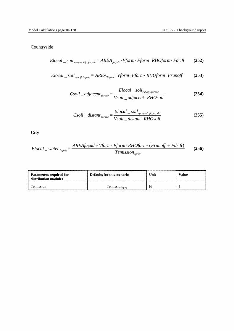
Model Calculations page III-128 EUSES 2.1 background report
Parameters required for distribution modules
Defaults for this scenario Unit Value
Temission Temissionspary [d] 1
Countryside
FdriftRHOformFformVform AREA = soilElocal adefaadefadriftspray ⋅⋅⋅⋅− çç,_ (252)
FrunoffRHOformFformVform AREA = soilElocal façadefaçaderunoff, ⋅⋅⋅⋅_ (253)
RHOsoiladjacentVsoil
soilElocal = adjacentCsoil façaderunoff
façade ⋅__
_ , (254)
RHOsoildistantsoilV
soilElocal = distantsoilC façadedriftspray
façade ⋅−
__
_ , (255)
City
sprayfaçade Temission
FdriftFrunoffRHOformFformVform façadeAREA = waterElocal )(_ +⋅⋅⋅⋅ (256)

EUSES 2.1 background report Model Calculations page III-129
Input COMB Simultaneous treatment of roof and façade [yes/no] P AREAfaçade façade area treated per day [m2] D Vform fluid application rate of applied formulation [m3.m-2] S RHOproduct density of formulation [kg.m-3] S/D Fform fraction of active ingredient in formulation [kgc.kg] S Fdrift fraction of product lost during application due to spray drift [-] D Frunoff fraction of product lost during application due to runoff [-] D Vsoil-adjacentfaçade volume of soil adjacent to treated object [m3] D Vsoil-distantfaçade volume of soil distant to treated object [m3] D RHOsoil bulk density of wet soil [kgwwt.m3] D Temissionspray number of emission days for spraying [d] D Elocal _soilspray-drift,façade local emission to soil from spray-drift, distant to façade [kgc] Oc
Elocal_soilrunoff,façade local emission to soil from runoff, adjacent to façade [kgc] Oc
Output Elocal_waterfaçade local emission to waste water during episode [kgc.d-1] O Csoil-adjacentfaçade local concentration in soil adjacent to façade [kgc.kgwwt
-1] O Csoil-distantfaçade local concentration in soil distant to façade [kgc.kgwwt
-1] O Temission number of emission days [d] O
Table III-96 Default settings for façade spraying. Parameter Symbol Unit Value
Simultaneous treatment of roof and façade COMB [yes/no] yes
Area of façade treated per day AREAfaçade [m2] 125
Fluid application rate of product Vform [m3.m-2] -
Fraction of active ingredient in product Fform [kgc.kg] -
Density of product RHOform [kg.m-3] 1000
Fraction of product lost by spray drift Fdrift [-] 0.1
Fraction of product lost due to runoff Frunoff [-] 0.2
Volume of soil adjacent to façade Vsoil-adjacentfaçade [m3] 0.5
Volume of soil distant to façade COMB = yes COMB = no
Vsoil-distantfaçade [m3]
54.1
27.3
Bulk density of wet soil RHOsoil [kgwwt.m-3] 1700
Number of emission days for spraying Temissionspray [d] 1
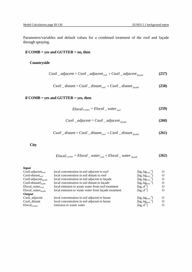
Model Calculations page III-130 EUSES 2.1 background report
Parameters/variables and default values for a combined treatment of the roof and façade through spraying.
Input Csoil-adjacentroof local concentration in soil adjacent to roof [kgc.kgwwt
-1] O Csoil-distantroof local concentration in soil distant to roof [kgc.kgwwt
-1] O Csoil-adjacentfaçade local concentration in soil adjacent to façade [kgc.kgwwt
-1] O Csoil-distantfaçade local concentration in soil distant to façade [kgc.kgwwt
-1] O Elocal_waterroof local emission to waste water from roof treatment [kgc.d-1] O Elocal_waterfaçade local emission to waste water from façade treatment [kgc.d-1] O
Output Csoil_adjacent local concentration in soil adjacent to house [kgc.kgwwt
-1] O Csoil_distant local concentration in soil adjacent to house [kgc.kgwwt
-1] O Elocal3,water emission to waste water [kgc.d-1] O
if COMB = yes and GUTTER = no, then
Countryside
façadeadjacentCsoiladjacentCsoil= adjacentCsoil ___ roof + (257)
façadedistantsoilCdistantsoilC = distantsoilC ___ roof + (258)
if COMB = yes and GUTTER = yes, then
waterElocal =Elocal water _ roof,3 (259)
façadeadjacentCsoil= adjacentCsoil __ (260)
façadedistantsoilCdistantsoilC = distantsoilC ___ roof + (261)
City
waterElocalwaterElocal =Elocal façadewater __ roof,3 + (262)
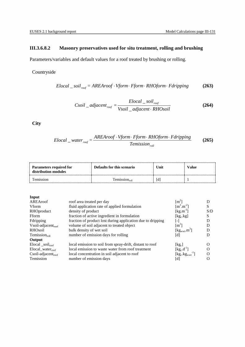
EUSES 2.1 background report Model Calculations page III-131
III.3.6.8.2 Masonry preservatives used for situ treatment, rolling and brushing Parameters/variables and default values for a roof treated by brushing or rolling.
Parameters required for distribution modules
Defaults for this scenario Unit Value
Temission Temissionroll [d] 1
Input AREAroof roof area treated per day [m2] D Vform fluid application rate of applied formulation [m3.m-2] S RHOproduct density of product [kg.m-3] S/D Fform fraction of active ingredient in formulation [kgc.kg] S Fdripping fraction of product lost during application due to dripping [-] D Vsoil-adjacentroof volume of soil adjacent to treated object [m3] D RHOsoil bulk density of wet soil [kgwwt.m3] D Temissionroll number of emission days for rolling [d] D Output Elocal _soilroof local emission to soil from spray-drift, distant to roof [kgc] O Elocal_waterroof local emission to waste water from roof treatment [kgc.d-1] O Csoil-adjacentroof local concentration in soil adjacent to roof [kgc.kgwwt
-1] O Temission number of emission days [d] O
Countryside
FdrippingRHOformFformVform AREAroof = soilElocal roof ⋅⋅⋅⋅_ (263)
RHOsoiladjacentVsoil
soilElocal = adjacentCsoil roof
roof ⋅__
_ (264)
City
roll
roof TemissionFdrippingRHOformFformVform AREAroof = waterElocal ⋅⋅⋅⋅_ (265)
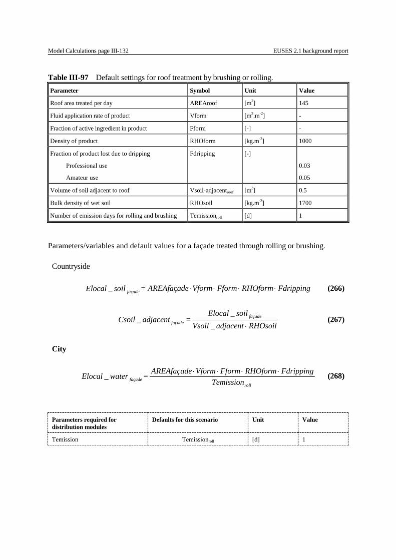
Model Calculations page III-132 EUSES 2.1 background report
Parameters/variables and default values for a façade treated through rolling or brushing.
Parameters required for distribution modules
Defaults for this scenario Unit Value
Temission Temissionroll [d] 1
Table III-97 Default settings for roof treatment by brushing or rolling. Parameter Symbol Unit Value
Roof area treated per day AREAroof [m2] 145
Fluid application rate of product Vform [m3.m-2] -
Fraction of active ingredient in product Fform [-] -
Density of product RHOform [kg.m-3] 1000
Fraction of product lost due to dripping
Professional use
Amateur use
Fdripping [-]
0.03
0.05
Volume of soil adjacent to roof Vsoil-adjacentroof [m3] 0.5
Bulk density of wet soil RHOsoil [kg.m-3] 1700
Number of emission days for rolling and brushing Temissionroll [d] 1
Countryside
FdrippingRHOformFformVform adeAREAfa = soilElocal adefa ⋅⋅⋅⋅ç_ ç (266)
RHOsoiladjacentVsoil
soilElocal = adjacentCsoil façade
façade ⋅__
_ (267)
City
roll
façade TemissionFdrippingRHOformFformVform façadeAREA = waterElocal ⋅⋅⋅⋅_ (268)
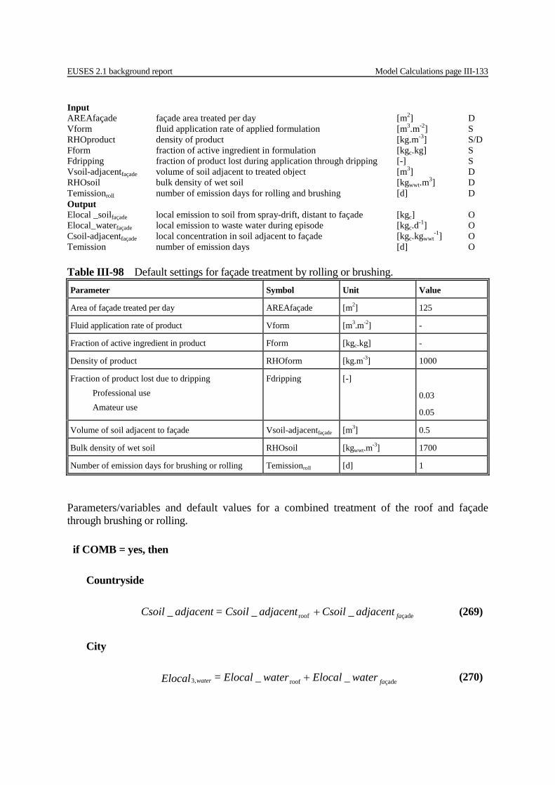
EUSES 2.1 background report Model Calculations page III-133
Input AREAfaçade façade area treated per day [m2] D Vform fluid application rate of applied formulation [m3.m-2] S RHOproduct density of product [kg.m-3] S/D Fform fraction of active ingredient in formulation [kgc.kg] S Fdripping fraction of product lost during application through dripping [-] S Vsoil-adjacentfaçade volume of soil adjacent to treated object [m3] D RHOsoil bulk density of wet soil [kgwwt.m3] D Temissionroll number of emission days for rolling and brushing [d] D Output Elocal _soilfaçade local emission to soil from spray-drift, distant to façade [kgc] O Elocal_waterfaçade local emission to waste water during episode [kgc.d-1] O Csoil-adjacentfaçade local concentration in soil adjacent to façade [kgc.kgwwt
-1] O Temission number of emission days [d] O
Parameters/variables and default values for a combined treatment of the roof and façade through brushing or rolling.
Table III-98 Default settings for façade treatment by rolling or brushing. Parameter Symbol Unit Value
Area of façade treated per day AREAfaçade [m2] 125
Fluid application rate of product Vform [m3.m-2] -
Fraction of active ingredient in product Fform [kgc.kg] -
Density of product RHOform [kg.m-3] 1000
Fraction of product lost due to dripping Professional use Amateur use
Fdripping [-]
0.03
0.05
Volume of soil adjacent to façade Vsoil-adjacentfaçade [m3] 0.5
Bulk density of wet soil RHOsoil [kgwwt.m-3] 1700
Number of emission days for brushing or rolling Temissionroll [d] 1
if COMB = yes, then
Countryside
çaderoof ___ faadjacentCsoiladjacentCsoil= adjacentCsoil + (269)
City
waterElocalwaterElocal =Elocal fawater __ çaderoof,3 + (270)
Model Calculations page III-134 EUSES 2.1 background report
Input Csoil-adjacentroof local concentration in soil adjacent to roof [kgc.kg-1] O Csoil-adjacentfaçade local concentration in soil adjacent to façade [kgc.kg-1] O Elocal_waterroof local emission to waste water from roof treatment [kgc.d-1] O Elocal_waterfaçade local emission to waste water from façade treatment [kgc.d-1] O Output Csoil_adjacent local concentration in soil adjacent to house [kgc.kg-1] O Elocal3,water emission to waste water [kgc.d-1] O
III.3.6.8.3 Masonry preservatives used for in- situ treatment, rinse Parameters/variables and default values for release during rinse with high pressure spraying. Release depends on the way of application to the substrate (i), either spraying or rolling and brushing. Relevant stage of the life cycle is waste treatment, stage 7.
Table III-99 Default settings for combined treatment of roof and façade by rolling or brushing.
Parameter Symbol Unit Value
Simultaneous treatment of roof and facade COMB [yes/no] yes
elimFFrunoffFdrift = Frinsespray −−−1 (271) elimFFdripping = Frinseroll −−1 (272) Countryside
if GUTTER = no, then
irinseroofdrift FrinseFdriftRHOformFformVform AREAroof = soilElocal ⋅⋅⋅⋅⋅_ , (273)
irinsefaçadedrift FrinseFdriftRHOformFformVform façadeAREA = soilElocal ⋅⋅⋅⋅⋅_ , (274)
irinseroofroofrunoff, FrinseFrunoffRHOformFformVform AREA = soilElocal ⋅⋅⋅⋅⋅_ (275)
irinsefaçaderunoff, FrinseFrunoffRHOformFformVform façadeAREA = soilElocal ⋅⋅⋅⋅⋅_ (276)

EUSES 2.1 background report Model Calculations page III-135
Parameters required for distribution modules
Defaults for this scenario Unit Value
Temission Temissionrinse [d] 1
Input Felim fraction of product eliminated between application and rinse [-] D Frinsespray fraction of product lost during rinse for spraying [-] Oc
Frinseroll fraction of product lost during rinse for rolling and brushing [-] Oc
Fdriftrinse fraction of product lost during rinse due to spray drift [-] D Frunoffrinse fraction of product lost during rinse due to runoff [-] D Temissionrinse number of emission days for rinsing [d] D Elocal _soildrift,roof local emission to soil from spray-drift due to roof rinse [kgc] Oc
Elocal _soildrift,façade local emission to soil from spray-drift due to façade rinse [kgc] Oc
Elocal_soilrunoff,roof local emission to soil from runoff, due to roof rinse [kgc] Oc
Elocal_soilrunoff, façade local emission to soil from runoff, due to rinse of façade, [kgc] Oc
Output Elocal7,water local emission to waste water due to rinse [kgc.d-1] O Csoil-adjacent local concentration in soil adjacent to building [kgc.kgwwt
-1] O Csoil-distant local concentration in soil distant to building [kgc.kgwwt
-1] O Temission number of emission days [d] D
RHOsoiladjacentVsoil
soilElocalsoilElocal = adjacentCsoil façaderunofftroofrunoff
⋅
+
___
_ ,, (277)
RHOsoildistantsoilV
soilElocalsoilElocal = distantsoilC façadedriftroofdrift
⋅
+
___
_ ,, (278)
if GUTTER = yes, then
rinse
irinsewater Temission
FrinseFrunoffRHOformFformVform AREAroof = Elocal
⋅⋅⋅⋅⋅,7 (279)
RHOsoiladjacentVsoil
soilElocal = adjacentCsoil façaderunoff
⋅__
_ , (280)
RHOsoildistantsoilV
soilElocalsoilElocal = distantsoilC façadedriftroofdrift
⋅
+
___
_ ,, (281)
City
rinse
iwater Temission
FrinseRHOformFformVform façadeAREAAREAroof = Elocal
⋅⋅⋅⋅+ )(,7 (282)
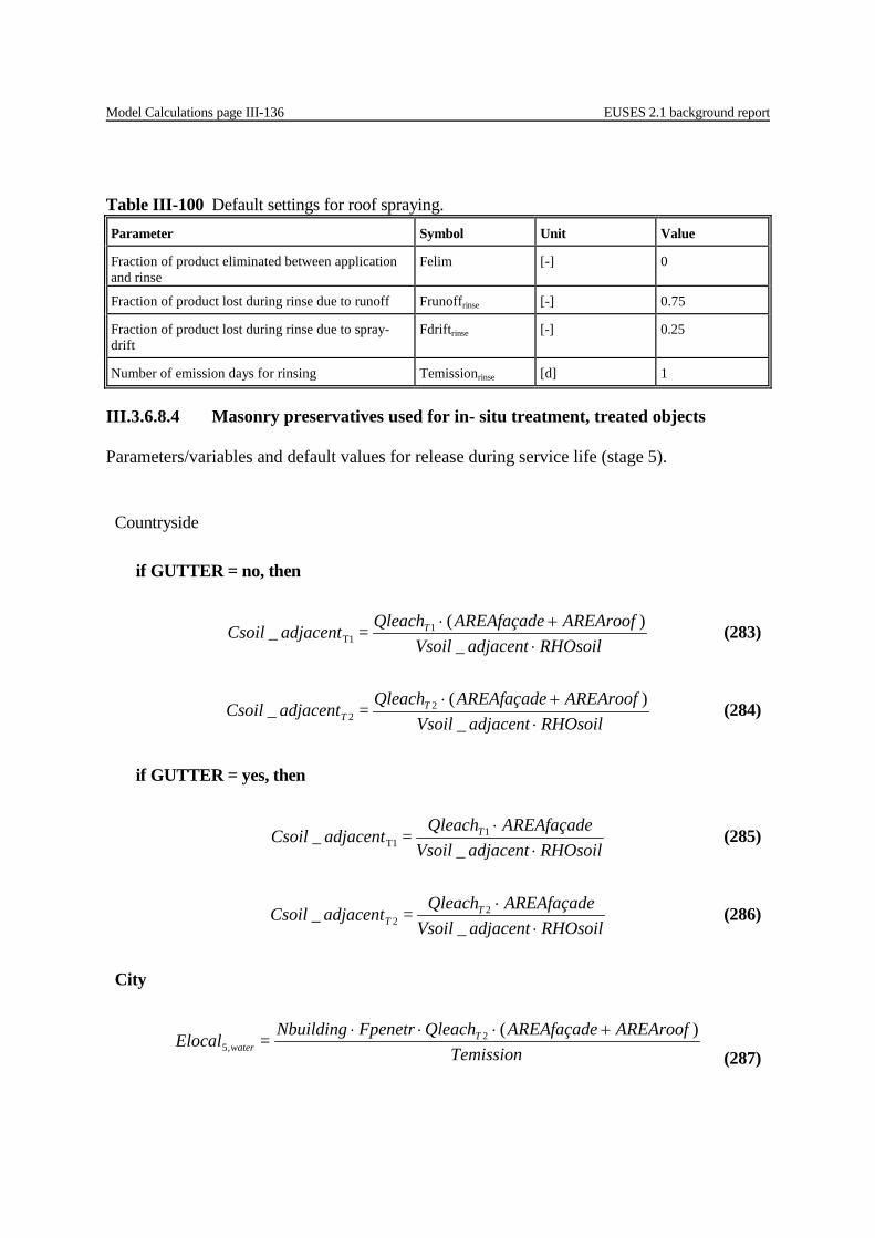
Model Calculations page III-136 EUSES 2.1 background report
III.3.6.8.4 Masonry preservatives used for in- situ treatment, treated objects Parameters/variables and default values for release during service life (stage 5).
Table III-100 Default settings for roof spraying. Parameter Symbol Unit Value
Fraction of product eliminated between application and rinse
Felim [-] 0
Fraction of product lost during rinse due to runoff Frunoffrinse [-] 0.75
Fraction of product lost during rinse due to spray-drift
Fdriftrinse [-] 0.25
Number of emission days for rinsing Temissionrinse [d] 1
Countryside
if GUTTER = no, then
RHOsoiladjacentVsoil
AREArooffaçadeAREAQleach = adjacentCsoil T
⋅+⋅
_)(_ 1
T1 (283)
RHOsoiladjacentsoilV
AREArooffaçadeAREAQleach = adjacentsoilC TT ⋅
+⋅_
)(_ 22 (284)
if GUTTER = yes, then
RHOsoiladjacentVsoilfaçadeAREAQleach = adjacentCsoil T
⋅⋅
__ 1
T1 (285)
RHOsoiladjacentsoilVfaçadeAREAQleach = adjacentsoilC T
T ⋅⋅
__ 2
2 (286)
City
TemissionAREArooffaçadeAREAQleachFpenetrNbuilding = Elocal T
water)(2
,5+⋅⋅⋅
(287)

EUSES 2.1 background report Model Calculations page III-137
Parameters required for distribution modules
Defaults for this scenario Unit Value
Temission Temissionini [d] 30
Temission Temissionchron [d] 365
Input GUTTER Building fitted with gutter [yes/no] P AREAfaçade treated roof area of building [m2] D AREAroof treated roof area of building [m2] D QleachtT1 cumulative quantity of active ingredient leached over the initial assessment period [kgc.m-2] S QleachtT2 cumulative quantity of active ingredient leached over the longer assessment period [kgc.m-2] S Temissionini Duration of the initial assessment period [d] D Temssionchron duration of the longer assessment period [d] D Vsoil-adjacent volume of soil adjacent to treated object [m3] D RHOsoil density of wet soil [kgwwt.m-3] Fpenetr penetration factor [-] D Nbuilding number of treated buildings in a city [-] D Elocal_waterT1 local emission to water from treated building at the countryside during the initial assessment period [kgc.d-1] Oc
Elocal_waterT2 local emission to water from treated building at the countryside during the longer assessment period [kgc.d-1] Oc
Output Elocal5,water local emission to waste water from treated buildings in a city [kgc.d-1] O Csoil-adjacentT1 local concentration in soil adjacent to façade [kgc.kgwwt
-1] O Csoil-distantT2 local concentration in soil distant to façade [kgc.kgwwt
-1] O Temission number of emission days [d] O
Table III-101 Default settings for façade spraying. Parameter Symbol Unit Value
Roof fitted with gutter GUTTER [yes/no] yes
Area of façade treated AREAfaçade [m2] 125
Area of façade treated AREAroof [m2] 145
Cumulative quantity of active ingredient leached over initial assessment period
QleachT1 [kg.m-2] -
Cumulative quantity of active ingredient leached over longer assessment period
QleachT2 [kg.m-2] -
Duration of the initial assessment period Temissionini [d] 30
Duration of the longer assessment period Temissionchron [d] >30
Bulk density of wet soil RHOsoil [kgwwt.m-3] 1700
Volume of soil adjacent to building Vsoil [-] 0.5
Penetration factor for product Fpenetr [-] 1
Number of treated buildings in a city Nbuilding [-] 1
Model Calculations page III-138 EUSES 2.1 background report
III.3.6.9 Product type 11: Preservatives for liquid-cooling and processing systems The scenarios and models and calculation formulations used in this version of EUSES 2.1.1 for Preservatives for liquid-cooling and processing systems have been taken from the following document:
− Supplement to the methodology for risk evaluation of biocides Harmonisation of Environmental Emission Scenarios for biocides used as preservatives for liquid cooling systems (product type 11) EC DG ENV / RIVM, 2003
This document can be obtained from the ECB Biocides website The following modifications are made:
− In order to determine the concentration in surface water depending on the river flow and the blow flow rate, additional equations have been added.
− Furthermore in addition to the original emission scenario the average emission and average concentration have been added to the calculations for the concentration at a certain point in time.
− Also different exposure time frames have been distinguished for the shock dosing scenarios e.g. the acute and chronic situation.
III.3.6.9.1 Biocides in process and cooling-water installations Industrial use Parameters/variables and default values for release from once-through systems Once-through systems can be modeled as plug-flow reactors. The plug leaves the system at the hydraulic residence time. The event lasts for a period which equals the dosing time period. Degradation does only take place during the time the plug is in the system, the hydraulic residence time. Repeated dosing can take place at regular time intervals, several times a day. In that case the average daily concentration in the blowdown should be estimated taking the number of dosings per day into account. For once-through systems release and the concentration are calculated for each dosing event, for the acute situation representing one emission day and the chronic situation representing 300 emission days. The blow down water can either be discharged directly to surface water or the public STP. The latter is usually only the case for small cooling systems. In case of direct discharge the concentration in surface water is directly calculated by applying a dilution factor. The dilution factor, for which no default value is given in the scenario, should be based on the discharge of the total number of cooling systems at the site, Ncool. General
QbldVsyst= HRT (288)
QbldN
QbldNFLOWDILUTION
cool
coolrivercooling ⋅
⋅+= (289)
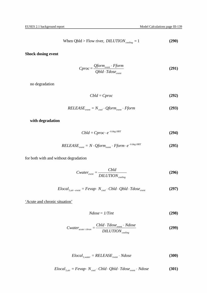
EUSES 2.1 background report Model Calculations page III-139
When Qbld > Flow river, 1= DILUTIONcooling (290)
Shock dosing event
event
event
TdoseQbldFformQform
= Cproc⋅
⋅ (291)
no degradation
Cproc = Cbld (292)
FformQformN = RELEASE eventcoolevent ⋅⋅ (293)
with degradation
HRTkeCproc = Cbld ⋅−⋅ deg (294)
HRTkeventevent eFformQform N= RELEASE ⋅−⋅⋅⋅ deg (295)
for both with and without degradation
cooling
event DILUTIONCbld = Cwater (296)
eventcooleventair TdoseQbldCbldNFevap = Elocal ⋅⋅⋅⋅−,3 (297)
‘Acute and chronic situation’
1/Tint= Ndose (298)
cooling
eventchronacute DILUTION
NdoseTdoseCbld = Cwater
⋅⋅/ (299)
NdoseRELEASE = Elocal eventwater ⋅,3 (300)
NdoseTdoseQbldCbldNFevap = Elocal eventcoolair ⋅⋅⋅⋅⋅,3 (301)
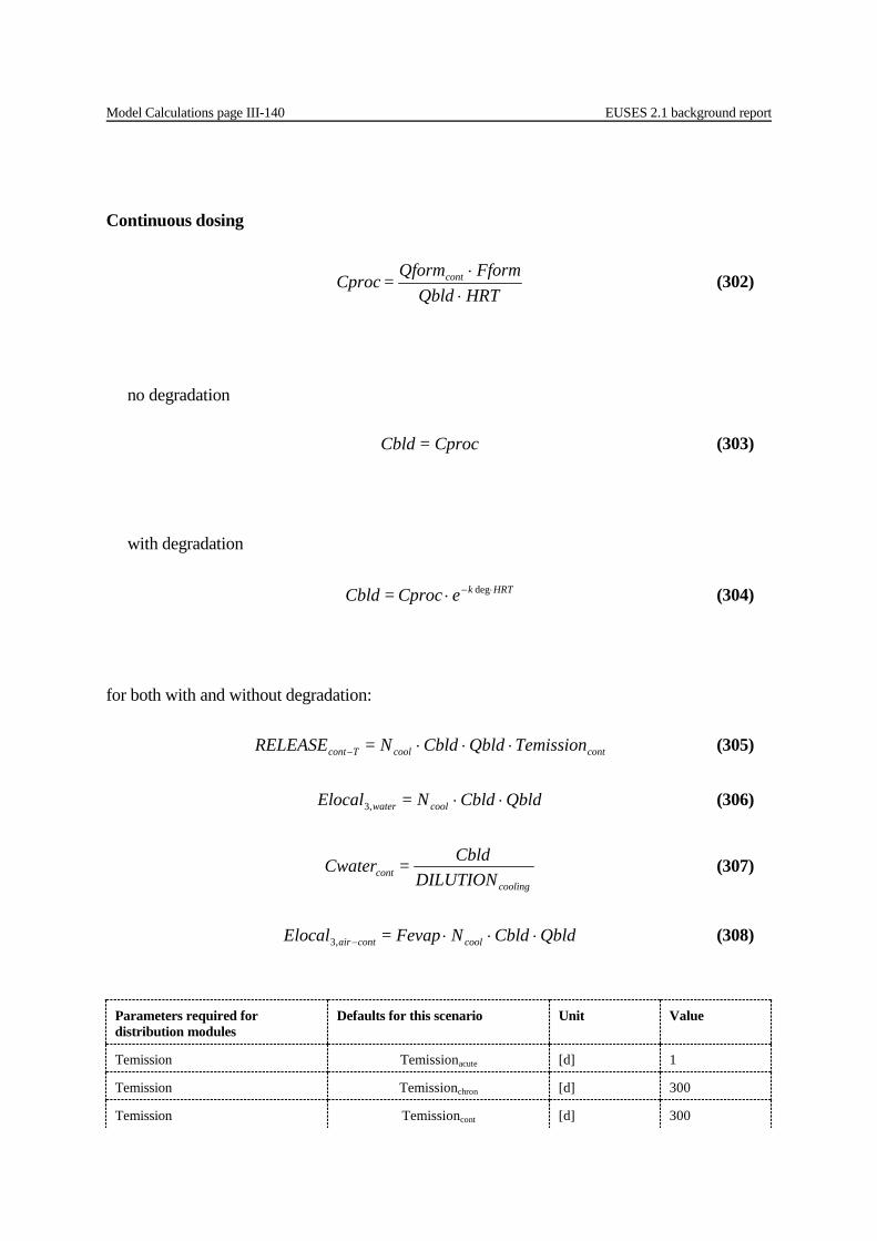
Model Calculations page III-140 EUSES 2.1 background report
Continuous dosing
HRTQbld
FformQform = Cproc cont
⋅⋅ (302)
no degradation
Cproc= Cbld (303)
with degradation
HRTkeCproc = Cbld ⋅−⋅ deg (304)
for both with and without degradation:
contcoolTcont TemissionQbldCbldN = RELEASE ⋅⋅⋅− (305)
QbldCbldN = Elocal coolwater ⋅⋅,3 (306)
cooling
cont DILUTIONCbld = Cwater (307)
QbldCbldNFevap = Elocal coolcontair ⋅⋅⋅−,3 (308)
Parameters required for distribution modules
Defaults for this scenario Unit Value
Temission Temissionacute [d] 1
Temission Temissionchron [d] 300
Temission Temissioncont [d] 300

EUSES 2.1 background report Model Calculations page III-141
Input Vsyst volume of water in cooling system [m3] D Qbld blowdown flow rate [m3.d-1] D Qformevent amount of product used in shock dose treatment [kg] S Qformcont amount of product applied in continuous treatment during a time period = HRT [kg] S Fform fraction of substance in the used product [kgc.kg-1] S Tdoseevent duration of shock dosing event [d] D Ncool number of cooling systems per site [-] D kdeg degradation rate constant [d-1] S HRT hydraulic residence time [d] Oc Cproc concentration in cooling water of the cooling system [kgc.m-3] O Fevap fraction of water lost due to evaporation [-] D Cbld concentration in blow down water [kgc.m-3] O Cproc concentration in cooling water of the cooling system [kgc.m-3] O Ndose number of dosings per day [d-1] O Tint dosing time interval [d] S FLOWriver river flow rate [m3.d-1] S DILUTIONcooling dilution factor in receiving surface water for the total number of cooling systems (Ncool) [-] O/S Temissioncont number of emission days per year [d] O Output RELEASEevent release from a shock dosing event [kgc] O Elocal3,air-event local emission to air at shock dose treatment event [kg.d-1] O RELEASEcont-T continuous release of substance over time period T [kgc] O Elocal3,air-cont local emission to air from continuous dosing [kg.d-1] Cwaterevent concentration of chemical in surface water during shock dosing event [kgc.m-3] O Cwateracute/chron concentration of chemical in surface water [kgc.m-3] O Cwatercont average concentration in surface water over T days [kgc.m-3] O Table III-102 Default settings of the model for biocides used in once-through process and
cooling-water installations. Parameter Symbol Unit Value
Volume of water in cooling system Vsyst [m3] 6 000
Blow down flow rate Qbld [m3.d-1] 576 000
amount of product used in shock dose treatment Qformevent [kg] -
Fraction of substance in the applied product Fform [kgc.kg-1] -
Duration of shock dose event Tdoseevent [d] 0.01042
Number of cooling systems per site Ncool [-] 2
Degradation rate constant kdeg [d-1] -
Fraction of water lost due to evaporation Fevap [-] 0.01
Flow rate of receiving surface water FLOWriver [-] -
Dilution factor for receiving surface water DILUTIONcooling [-] -
Parameters/variables and default values for release from open recirculation systems Open recirculation systems can be modeled as a continuously ideally stirred tank reactor when assuming that the recirculation flow rate (Qcirc) is much larger than the blow down
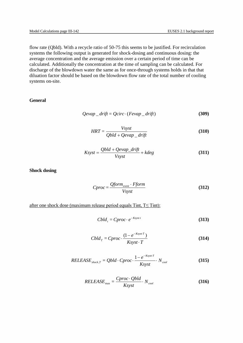
Model Calculations page III-142 EUSES 2.1 background report
flow rate (Qbld). With a recycle ratio of 50-75 this seems to be justified. For recirculation systems the following output is generated for shock-dosing and continuous dosing: the average concentration and the average emission over a certain period of time can be calculated. Additionally the concentration at the time of sampling can be calculated. For discharge of the blowdown water the same as for once-through systems holds in that that diluation factor should be based on the blowdown flow rate of the total number of cooling systems on-site.
General
)_(_ driftFevapQcirc= driftQevap ⋅ (309)
driftQevapQbld
Vsyst= HRT_+
(310)
kdegVsyst
tQevap_drifQbldKsyst ++
= (311)
Shock dosing
Vsyst
FformQform = Cproc event ⋅ (312)
after one shock dose (maximum release period equals Tint, T≤ Tint):
tKsystt eCproc = Cbld ⋅−⋅ (313)
TKsyst
eCproc = CbldTKsyst
T ⋅−
⋅⋅− )1( (314)
cool
TKsyst
Tshock NKsyste CprocQbld= RELEASE ⋅
−⋅⋅
⋅−1, (315)
coolNKsyst
Qbld Cproc= RELEASE ⋅⋅
max (316)
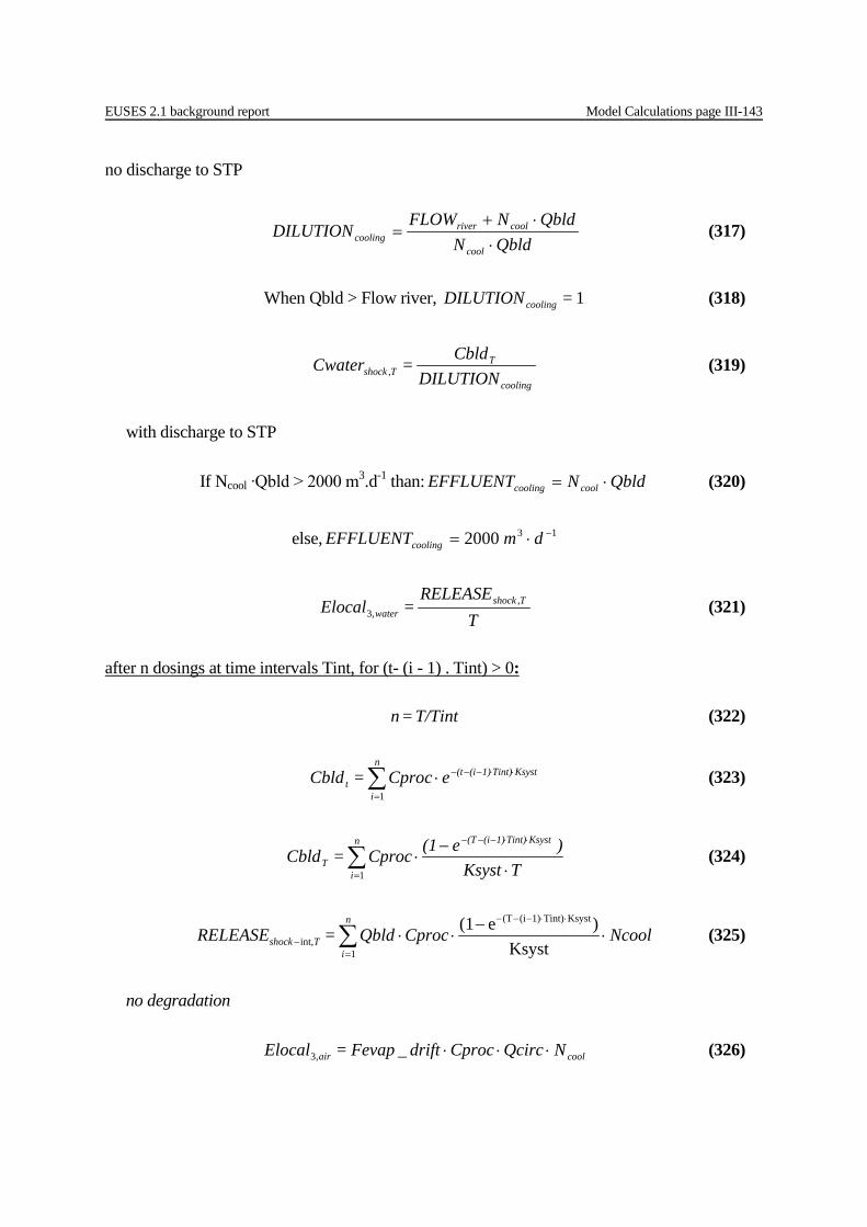
EUSES 2.1 background report Model Calculations page III-143
no discharge to STP
QbldN
QbldNFLOWDILUTION
cool
coolrivercooling ⋅
⋅+= (317)
When Qbld > Flow river, 1= DILUTIONcooling (318)
cooling
TTshock DILUTION
Cbld = Cwater , (319)
with discharge to STP
If Ncool ∙Qbld > 2000 m3.d-1 than: QbldNEFFLUENT coolcooling ⋅= (320)
else, 132000 −⋅= dmEFFLUENTcooling
T
RELEASE = Elocal Tshock
water,
,3 (321)
after n dosings at time intervals Tint, for (t- (i - 1) . Tint) > 0:
T/Tint = n (322)
∑=
⋅⋅−−−⋅n
i
KsystTint)1)(i(tt ecCpro = Cbld
1
(323)
∑=
⋅⋅−−−
⋅−
⋅n
i
KsystTint)1)(i(T
T TKsyst)e(1Cproc = Cbld
1
(324)
∑=
⋅⋅−−−
− ⋅−
⋅⋅n
iTshock NcoolCprocQbld = RELEASE
1
KsystTint)1)(i(T
int, Ksyst)e(1 (325)
no degradation
coolair NQcircCprocdriftFevap = Elocal ⋅⋅⋅_,3 (326)
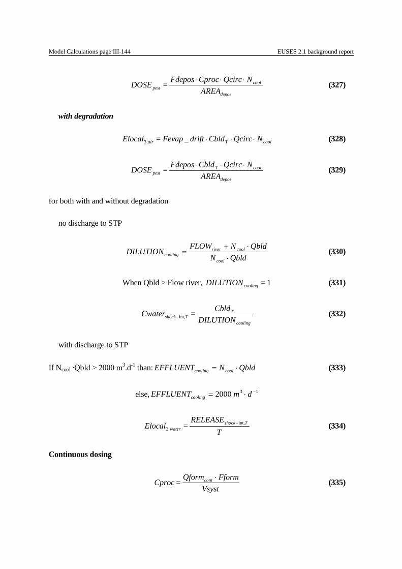
Model Calculations page III-144 EUSES 2.1 background report
depos
coolpest AREA
NQcircCprocFdepos = DOSE
⋅⋅⋅ (327)
with degradation
coolTair NQcircCblddriftFevap = Elocal ⋅⋅⋅_,3 (328)
depos
coolTpest AREA
NQcircCbldFdepos = DOSE
⋅⋅⋅ (329)
for both with and without degradation
no discharge to STP
QbldN
QbldNFLOWDILUTION
cool
coolrivercooling ⋅
⋅+= (330)
When Qbld > Flow river, 1= DILUTIONcooling (331)
cooling
TTshock DILUTION
Cbld = Cwater int,− (332)
with discharge to STP
If Ncool ∙Qbld > 2000 m3.d-1 than: QbldNEFFLUENT coolcooling ⋅= (333)
else, 132000 −⋅= dmEFFLUENTcooling
T
RELEASE = Elocal Tshock
waterint,
,3− (334)
Continuous dosing
Vsyst
FformQform = Cproc cont ⋅ (335)

EUSES 2.1 background report Model Calculations page III-145
HRTKsyst
Cproc = Cbld init
⋅+1 (336)
TQbldCbldN = RELEASE coolTcont ⋅⋅⋅, (337)
no degradation
coolair NQcircCprocdriftFevap = Elocal ⋅⋅⋅−,3 (338)
depos
coolpest AREA
NQcircCprocFdepos = DOSE
⋅⋅⋅ (339)
with degradation
coolair NQcircCblddriftFevap = Elocal ⋅⋅⋅_,3 (340)
depos
coolpest AREA
NQcircCbldFdepos = DOSE
⋅⋅⋅ (341)
no discharge to STP
QbldN
QbldNFLOWDILUTION
cool
coolrivercooling ⋅
⋅+= (342)
When Qbld > Flow river, 1= DILUTIONcooling (343)
cooling
cont DILUTIONCbld = Cwater (344)
with discharge to STP
If Ncool ∙Qbld > 2000 m3.d-1 than: QbldNEFFLUENT coolcooling ⋅= (345)
else, 132000 −⋅= dmEFFLUENTcooling
T
RELEASE = Elocal Tcont
water,
,3 (346)
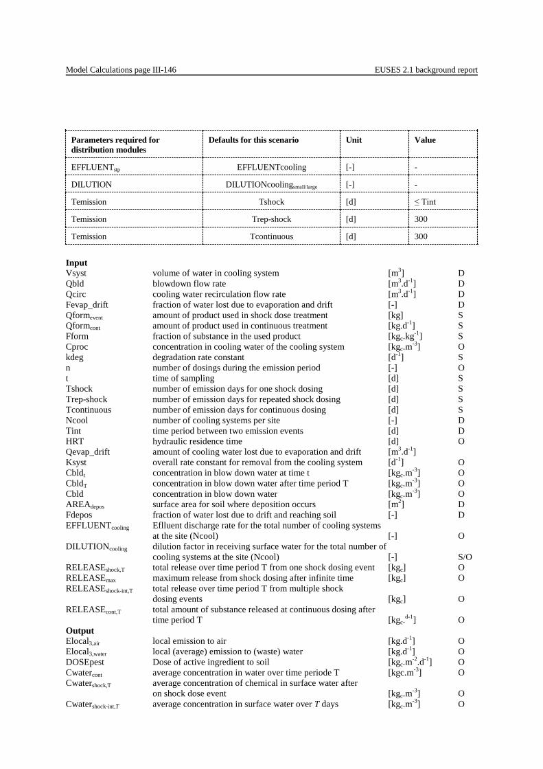
Model Calculations page III-146 EUSES 2.1 background report
Parameters required for distribution modules
Defaults for this scenario Unit Value
EFFLUENTstp EFFLUENTcooling [-] -
DILUTION DILUTIONcoolingsmall/large [-] -
Temission Tshock [d] ≤ Tint
Temission Trep-shock [d] 300
Temission Tcontinuous [d] 300
Input Vsyst volume of water in cooling system [m3] D Qbld blowdown flow rate [m3.d-1] D Qcirc cooling water recirculation flow rate [m3.d-1] D Fevap_drift fraction of water lost due to evaporation and drift [-] D Qformevent amount of product used in shock dose treatment [kg] S Qformcont amount of product used in continuous treatment [kg.d-1] S Fform fraction of substance in the used product [kgc.kg-1] S Cproc concentration in cooling water of the cooling system [kgc.m-3] O kdeg degradation rate constant [d-1] S n number of dosings during the emission period [-] O t time of sampling [d] S Tshock number of emission days for one shock dosing [d] S Trep-shock number of emission days for repeated shock dosing [d] S Tcontinuous number of emission days for continuous dosing [d] S Ncool number of cooling systems per site [-] D Tint time period between two emission events [d] D HRT hydraulic residence time [d] O Qevap_drift amount of cooling water lost due to evaporation and drift [m3.d-1] Ksyst overall rate constant for removal from the cooling system [d-1] O Cbldt concentration in blow down water at time t [kgc.m-3] O CbldT concentration in blow down water after time period T [kgc.m-3] O Cbld concentration in blow down water [kgc.m-3] O AREAdepos surface area for soil where deposition occurs [m2] D Fdepos fraction of water lost due to drift and reaching soil [-] D EFFLUENTcooling Eflluent discharge rate for the total number of cooling systems at the site (Ncool) [-] O DILUTIONcooling dilution factor in receiving surface water for the total number of cooling systems at the site (Ncool) [-] S/O RELEASEshock,T total release over time period T from one shock dosing event [kgc] O RELEASEmax maximum release from shock dosing after infinite time [kgc] O RELEASEshock-int,T total release over time period T from multiple shock dosing events [kgc] O RELEASEcont,T total amount of substance released at continuous dosing after time period T [kgc.d-1] O Output Elocal3,air local emission to air [kg.d-1] O Elocal3,water local (average) emission to (waste) water [kg.d-1] O DOSEpest Dose of active ingredient to soil [kgc.m-2.d-1] O Cwatercont average concentration in water over time periode T [kgc.m-3] O Cwatershock,T average concentration of chemical in surface water after on shock dose event [kgc.m-3] O Cwatershock-int,T average concentration in surface water over T days [kgc.m-3] O

EUSES 2.1 background report Model Calculations page III-147
Table III-103 Default settings of the model for biocides used in small and large open
recirculation process and cooling-water installations. Parameter Symbol Unit Value
large small
Volume of water in cooling system Vsyst [m3] 3 000 300
Blow down flow rate Qbld [m3.d-1] 3 000 48
Recirculation flow rate for cooling water Qcirc [m3.d-1] 216 000 2 400
Fraction of water released due to evaporation and drift Fevap_drift [-] 0.01 0.01
amount of product used in shock dose treatment Qformevent [kg] -
Number of cooling systems per site Ncool [-] 2
Time period between two emission event Tint [d] 1
Fraction of water lost due to drift and reaching soil Fdepos [-] 0.00025
Soil surface area where deposition occurs AREAdepos [m2] 100
Dilution factor for receiving surface water DILUTIONcooling [-]
Parameters/variables and default values for release from closed systems Single dosing
Vsyst
FformQform = Cproc event ⋅ (347)
QbldVsystHRT = (348)
deg1 kHRT
Ksyst += (349)
after one shock dose (maximum release period equals Tint, T≤ Tint):
tKsystt eCproc = Cbld ⋅−⋅ (350)
TKsyst
eCproc = CbldTKsyst
T ⋅−
⋅⋅−1 (351)
NcoolKsysteQbld Cproc= RELEASE
TKsyst
Tshock ⋅−
⋅⋅⋅−1
, (352)
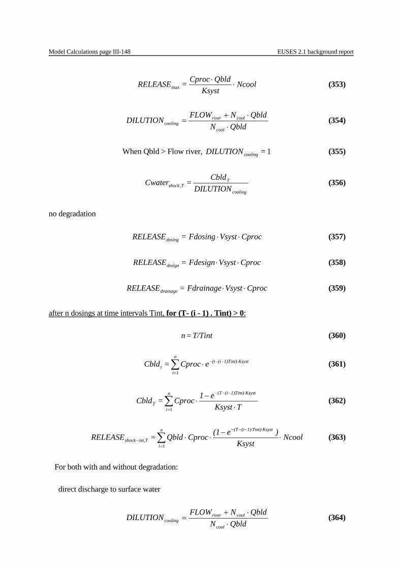
Model Calculations page III-148 EUSES 2.1 background report
NcoolKsyst
Qbld Cproc= RELEASE ⋅⋅
max (353)
QbldN
QbldNFLOWDILUTION
cool
coolrivercooling ⋅
⋅+= (354)
When Qbld > Flow river, 1= DILUTIONcooling (355)
cooling
TTshock DILUTION
Cbld = Cwater , (356)
no degradation
CprocVsystFdosing= RELEASEdosing ⋅⋅ (357)
CprocVsystFdesign= RELEASEdesign ⋅⋅ (358)
CprocVsystFdrainage= RELEASEdrainage ⋅⋅ (359)
after n dosings at time intervals Tint, for (T- (i - 1) . Tint) > 0:
T/Tint = n (360)
∑=
⋅−−−⋅n
i
Ksyst1)Tint)(i(tt eCproc = Cbld
1
(361)
∑=
⋅−−−
⋅−
⋅n
i
Ksyst1)Tint)(i(T
T TKsyste1Cproc = Cbld
1
(362)
∑=
⋅⋅−−−
− ⋅−
⋅⋅n
i
KsystTint)1)(i(T
Tshock NcoolKsyst
)e(1CprocQbld = RELEASE1
int, (363)
For both with and without degradation:
direct discharge to surface water
QbldN
QbldNFLOWDILUTION
cool
coolrivercooling ⋅
⋅+= (364)
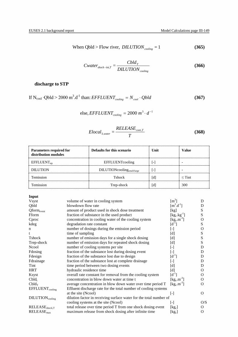
EUSES 2.1 background report Model Calculations page III-149
When Qbld > Flow river, 1= DILUTIONcooling (365)
cooling
TTshock DILUTION
Cbld = Cwater int,− (366)
discharge to STP
If Ncool ∙Qbld > 2000 m3.d-1 than: QbldNEFFLUENT coolcooling ⋅= (367)
else, 132000 −⋅= dmEFFLUENTcooling
T
RELEASE = Elocal Tcont
water,
,3 (368)
Parameters required for distribution modules
Defaults for this scenario Unit Value
EFFLUENTstp EFFLUENTcooling [-] -
DILUTION DILUTIONcoolingsmall/large [-] -
Temission Tshock [d] ≤ Tint
Temission Trep-shock [d] 300
Input Vsyst volume of water in cooling system [m3] D Qbld blowdown flow rate [m3.d-1] D Qformevent amount of product used in shock dose treatment [kg] S Fform fraction of substance in the used product [kgc.kg-1] S Cproc concentration in cooling water of the cooling system [kgc.m-3] O kdeg degradation rate constant [d-1] S n number of dosings during the emission period [-] O t time of sampling [d] S Tshock number of emission days for a single shock dosing [d] S Trep-shock number of emission days for repeated shock dosing [d] S Ncool number of cooling systems per site [-] D Fdosing fraction of the substance lost during dosing event [-] D Fdesign fraction of the substance lost due to design [d-1] D Fdrainage fraction of the substance lost at complete drainage [-] D Tint time period between two dosing events [d] D HRT hydraulic residence time [d] O Ksyst overall rate constant for removal from the cooling system [d-1] O Cbldt concentration in blow down water at time t [kgc.m-3] O CbldT average concentration in blow down water over time period T [kgc.m-3] O EFFLUENTcooling Eflluent discharge rate for the total number of cooling systems at the site (Ncool) [-] O DILUTIONcooling dilution factor in receiving surface water for the total number of cooling systems at the site (Ncool) [-] O/S RELEASEshock,T total release over time period T from one shock dosing event [kgc] O RELEASEmax maximum release from shock dosing after infinite time [kgc] O
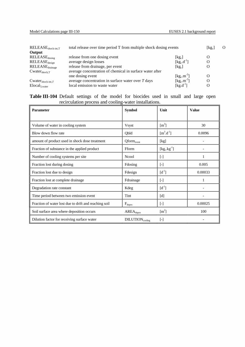
Model Calculations page III-150 EUSES 2.1 background report
RELEASEshock-int,T total release over time period T from multiple shock dosing events [kgc] O Output RELEASEdosing release from one dosing event [kgc] O RELEASEdesign average design losses [kgc.d-1] O RELEASEdrainage release from drainage, per event [kgc] O Cwatershock,T average concentration of chemical in surface water after one dosing event [kgc.m-3] O Cwatershock-int,T average concentration in surface water over T days [kgc.m-3] O Elocal3,water local emission to waste water [kg.d-1] O Table III-104 Default settings of the model for biocides used in small and large open
recirculation process and cooling-water installations. Parameter Symbol Unit Value
Volume of water in cooling system Vsyst [m3] 30
Blow down flow rate Qbld [m3.d-1] 0.0096
amount of product used in shock dose treatment Qformevent [kg] -
Fraction of substance in the applied product Fform [kgc.kg-1] -
Number of cooling systems per site Ncool [-] 1
Fraction lost during dosing Fdosing [-] 0.005
Fraction lost due to design Fdesign [d-1] 0.00033
Fraction lost at complete drainage Fdrainage [-] 1
Degradation rate constant Kdeg [d-1] -
Time period between two emission event Tint [d] -
Fraction of water lost due to drift and reaching soil Fdepos [-] 0.00025
Soil surface area where deposition occurs AREAdepos [m2] 100
Dilution factor for receiving surface water DILUTIONcooling [-] -
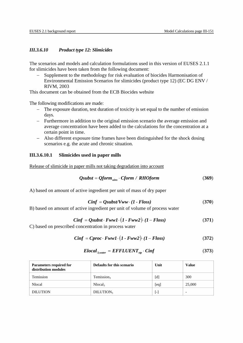
EUSES 2.1 background report Model Calculations page III-151
III.3.6.10 Product type 12: Slimicides The scenarios and models and calculation formulations used in this version of EUSES 2.1.1 for slimicides have been taken from the following document:
− Supplement to the methodology for risk evaluation of biocides Harmonisation of Environmental Emission Scenarios for slimicides (product type 12) (EC DG ENV / RIVM, 2003
This document can be obtained from the ECB Biocides website The following modifications are made:
− The exposure duration, test duration of toxicity is set equal to the number of emission days.
− Furthermore in addition to the original emission scenario the average emission and average concentration have been added to the calculations for the concentration at a certain point in time.
− Also different exposure time frames have been distinguished for the shock dosing scenarios e.g. the acute and chronic situation.
III.3.6.10.1 Slimicides used in paper mills Release of slimicide in paper mills not taking degradation into account RHOform / CformQformQsubst uins ⋅= (369) A) based on amount of active ingredient per unit of mass of dry paper Floss)-(1Qsubst/VwwCinf ⋅= (370) B) based on amount of active ingredient per unit of volume of process water ( ) Floss)(1Fww2-1Fww1QsubstCinf −⋅⋅⋅= (371) C) based on prescribed concentration in process water ( ) Floss)(1Fww2-1Fww1CprocCinf −⋅⋅⋅= (372) CinfEFFLUENTElocal stpwater3, ⋅= (373)
Parameters required for distribution modules
Defaults for this scenario Unit Value
Temission Temission3 [d] 300
Nlocal Nlocal3 [eq] 25,000
DILUTION DILUTION3 [-] -
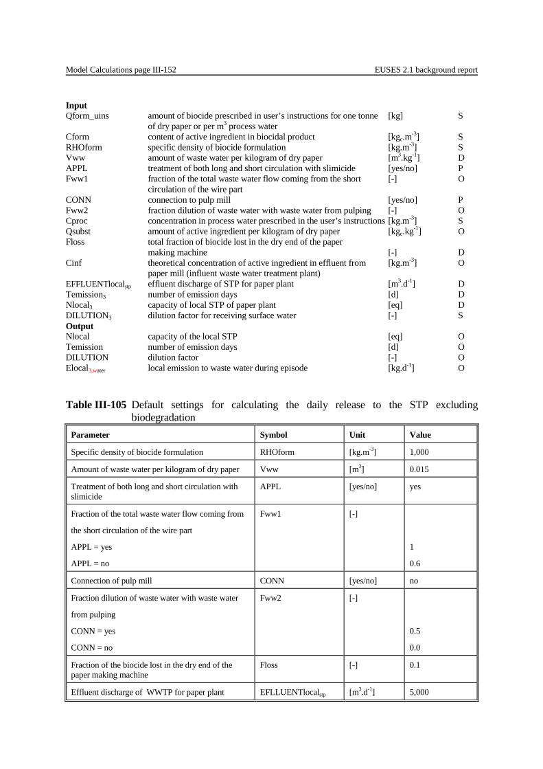
Model Calculations page III-152 EUSES 2.1 background report
Input Qform_uins amount of biocide prescribed in user’s instructions for one tonne [kg] S of dry paper or per m3 process water Cform content of active ingredient in biocidal product [kgc.m-3] S RHOform specific density of biocide formulation [kg.m-3] S Vww amount of waste water per kilogram of dry paper [m3.kg-1] D APPL treatment of both long and short circulation with slimicide [yes/no] P Fww1 fraction of the total waste water flow coming from the short [-] O circulation of the wire part CONN connection to pulp mill [yes/no] P Fww2 fraction dilution of waste water with waste water from pulping [-] O Cproc concentration in process water prescribed in the user’s instructions [kg.m-3] S Qsubst amount of active ingredient per kilogram of dry paper [kgc.kg-1] O Floss total fraction of biocide lost in the dry end of the paper making machine [-] D Cinf theoretical concentration of active ingredient in effluent from [kg.m-3] O paper mill (influent waste water treatment plant) EFFLUENTlocalstp effluent discharge of STP for paper plant [m3.d-1] D Temission3 number of emission days [d] D Nlocal3 capacity of local STP of paper plant [eq] D DILUTION3 dilution factor for receiving surface water [-] S Output Nlocal capacity of the local STP [eq] O Temission number of emission days [d] O DILUTION dilution factor [-] O Elocal3,water local emission to waste water during episode [kg.d-1] O Table III-105 Default settings for calculating the daily release to the STP excluding
biodegradation Parameter Symbol Unit Value
Specific density of biocide formulation RHOform [kg.m-3] 1,000
Amount of waste water per kilogram of dry paper Vww [m3] 0.015
Treatment of both long and short circulation with slimicide
APPL [yes/no] yes
Fraction of the total waste water flow coming from
the short circulation of the wire part
APPL = yes
APPL = no
Fww1 [-]
1
0.6
Connection of pulp mill CONN [yes/no] no
Fraction dilution of waste water with waste water
from pulping
CONN = yes
CONN = no
Fww2 [-]
0.5
0.0
Fraction of the biocide lost in the dry end of the paper making machine
Floss [-] 0.1
Effluent discharge of WWTP for paper plant EFLLUENTlocalstp [m3.d-1] 5,000
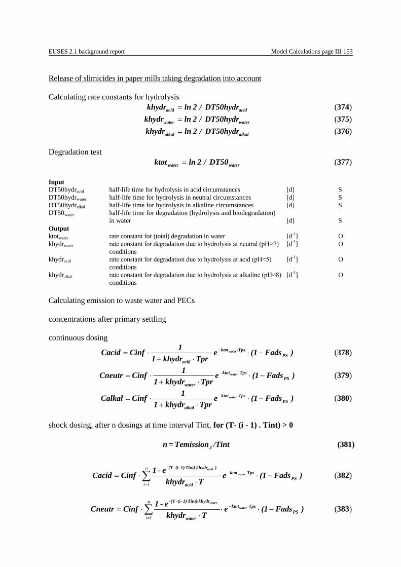
EUSES 2.1 background report Model Calculations page III-153
Release of slimicides in paper mills taking degradation into account Calculating rate constants for hydrolysis acidacid DT50hydr / 2lnkhydr = (374) waterwater DT50hydr / 2lnkhydr = (375) alkalalkal DT50hydr / 2lnkhydr = (376) Degradation test waterwater DT50 / 2lnktot = (377) Input DT50hydracid half-life time for hydrolysis in acid circumstances [d] S DT50hydrwater half-life time for hydrolysis in neutral circumstances [d] S DT50hydralkal half-life time for hydrolysis in alkaline circumstances [d] S DT50water half-life time for degradation (hydrolysis and biodegradation) in water [d] S Output ktotwater rate constant for (total) degradation in water [d-1] O khydrwater rate constant for degradation due to hydrolysis at neutral (pH≈7) [d-1] O conditions khydracid rate constant for degradation due to hydrolysis at acid (pH≈5) [d-1] O conditions khydralkal rate constant for degradation due to hydrolysis at alkaline (pH≈8) [d-1] O conditions Calculating emission to waste water and PECs concentrations after primary settling continuous dosing
)Fads(1eTprkhydr1
1CinfCacid PSTpsktot
acid
water −⋅⋅⋅+
⋅= ⋅− (378)
)Fads(1eTprkhydr1
1CinfCneutr PSTpsktot
water
water −⋅⋅+
⋅= ⋅− (379)
)Fads(1eTprkhydr1
1CinfCalkal PSTpsktot
alkal
water −⋅⋅+
⋅= ⋅− (380)
shock dosing, after n dosings at time interval Tint, for (T- (i - 1) . Tint) > 0 /TintTemission= n 3 (381)
)Fads(1eTkhydr
e-1CinfCacid PSTpsktot
acid
)khydrTint)1)-(i--(Twater
acid
−⋅⋅⋅
⋅= ⋅−
=
⋅⋅
∑n
i 1
(382)
)Fads(1eTkhydr
e-1CinfCneutr PSTpsktot
water
khydrTint)1)-(i--(Twater
water
−⋅⋅⋅
⋅= ⋅−
=
⋅⋅
∑n
i 1
(383)
Model Calculations page III-154 EUSES 2.1 background report
)Fads(1eTkhydr
e-1CinfCalkal PSTpsktot
alkal
)khydrTint)1)-(i--(Twater
alkal
−⋅⋅⋅
⋅= ⋅−
=
⋅⋅
∑n
i 1
(384)
general calculation for both continuous and shock dosing concentrations after chemical/mechanical treatment (worst case) )Fads(1eCacidCacid CM
TcmktotCM
water −⋅⋅= ⋅− (385) )Fads(1eCneutrCneutr CM
TcmktotCM
water −⋅⋅= ⋅− (386) )Fads(1eCalkalCalkal CM
Tcm)ktotCM
water −⋅⋅= ⋅− (387) Clocal in receiving surface water after chemical/mechanical treatment DILUTIONCacidClocal CMcidCM_water_a ÷= (388) DILUTIONCneutrClocal CMeutrCM_water_n ÷= (389) DILUTIONCalkalClocal CMlkalCM_water_a ÷= (390) Emission to waste water after primary settling (typical case) CacidEFFLUENTElocal stpacidwater,3, ⋅= (391) CneutrEFFLUENTElocal stprwater,neut3, ⋅= (392) CalkalEFFLUENTElocal stpalkalwater,3, ⋅= (393)
Parameters required for distribution modules
Defaults for this scenario Unit Value
Temission Temission3 [d] 300
Temission T [d] -
Nlocal Nlocal3 [eq] 25,000
DILUTION DILUTION3 [-] -
Input Cinf theoretical concentration of active ingredient [kg.m-3] O Tpr retention time for paper making process [d] D Tps retention time for primary settling [d] D Tcm retention time for chemical/mechanical treatment [d] D FadsPS fraction of the biocide adsorbed to particles during primary settling [-] D FadsCM fraction of the biocide adsorbed to particles during chemical/mechanical treatment [-] D Cacid concentration after primary settling for acid process conditions [kg.m-3] O Cneutr concentration after primary settling for neutral process [kg.m-3] O conditions Calkal concentration after primary settling for alkaline process [kg.m-3] O conditions CacidCM concentration after chemical/mechanical treatment for acid [kg.m-3] O process conditions CneutrCM concentration after chemical/mechanical treatment for neutral [kg.m-3] O process conditions
EUSES 2.1 background report Model Calculations page III-155
CalkalCM concentration after chemical/mechanical treatment for alkaline [kg.m-3] O process conditions Temission3 Number of emission days [d] S Tint time period between two dosing events [d] S n number of dosings during the emission period [-] O EFFLUENTlocalstp effluent discharge of STP for paper plant [m3.d-1] D Temission3 number of emission days [d] D Nlocal3 capacity of local STP of paper plant [eq] D DILUTION3 dilution factor for receiving surface water [-] S Output ClocalCM_water_acid predicted Environmental Concentration in receiving surface [kg.m-3] O water after chemical/mechanical treatment for acid process conditions at paper making ClocalCM_water_alkal predicted Environmental Concentration in receiving surface [kg.m-3] O water after chemical/mechanical treatment for alkaline process conditions at paper making ClocalCM_water_neutr predicted Environmental Concentration in receiving surface [kg.m-3] O water after chemical/mechanical treatment for neutral process conditions at paper making Nlocal capacity of the local STP [eq] O Temission number of emission days [d] O DILUTION dilution factor [-] O Elocal3,water,acid local emission to waste water for acid process conditions [kg.d-1] O after primary settling only Elocal3,water,alkal local emission to waste water for alkaline process conditions [kg.d-1] O after primary settling only EClocal3,water,neutr local emission to waste water for neutral process conditions [kg.d-1] O after primary settling only Table III-106 Default settings for calculating the effluent concentrations for on-site treatment
and influent concentrations for the STP. Parameter Symbol Unit Value
Retention time for the paper making process Tpr [d] 0.167
Retention time for primary settling Tps [d] 0.167
Retention time for chemical/mechanical treatment Tcm [d] 0.167
Fraction of the slimicide adsorbed to particles during primary settling
FadsPS [-] 0
Fraction of the biocide adsorbed to particles during chemical/mechanical treatment
FadsCM [-] 0
III.3.6.10.2 Slimicides used in oil extraction processes Model for release from oil extraction platforms A) based on the fraction of active ingredient in drilling mud RHOmudVmudFsubst_muderRELEASEwat ⋅⋅= (394) B) based on amount of active ingredient per unit of volume of drilling mud FconvVmudQsubst_muderRELEASEwat ⋅⋅= (395)

Model Calculations page III-156 EUSES 2.1 background report
A/B) _wwayDEPTHlocaltform1/DENSEplaVwaterplatform ⋅= (396) waterplatformwater FreplVwaterVrepl ⋅= (397) Continuous discharge
water
contwater, VreplTdrillerRELEASEwatPEClocal
⋅= (398)
Tintkdeg
sedsede1Fdeg ⋅−−= (399)
)Fdeg(1KpPEClocalPEClocal sedsedcontwater,sediment −⋅⋅= (400) Batchwise discharge
batch
batchwater, DILUTIONVmuderRELEASEwatPEClocal
⋅= (401)
Parameters/variables and default values for release from oil extraction platforms Input - Type of discharge [-] P - size of the section [-] P Vmud volume of mud discharged from a specific section [m3] D Fsubst_mud fraction of substance in the mud [kgc.kg-1] S RHOmud density of the discharged drilling mud [kg.m-3] D Qsubst_mud amount of substance in drilling mud [pound.barrel-1] S Fconv conversion factor from pounds per barrel to kg.m-3 [1)] Dc
DENSEplatform number of platforms per square kilometer [km-2] DDEPTHlocal_water average depth of water around platform [m] D Freplwater fraction of sea water refreshed in the receiving volume around the platform per day [d-1] D Tdrill drilling time for a section [d] D DILUTIONbatch dilution factor for batch wise discharges [-] D Kpsed sediment water partition coefficient [m-3.kg-1] Oc Vwaterplatform volume of water around a platform [m-3] O Vreplwater volume of water passing the platform [m3.d-1] O RELEASEwater local release of substance to sea water per drilling period [kgc] O CONVsed conversion factor for sediment concentrations: wwt to dwt [kgwwt.kgdwt
-1] O] kdegsed first order degradation rate in sediment [d-1] S Tint long term interval for sediment concentration [d] D Fdegsed fraction of substance in sediment degraded after one year [-] O Kpsed sediment water partition coefficient [m3.kg-1] O

EUSES 2.1 background report Model Calculations page III-157
Output PECwater,cont predicted environmental concentration in receiving sea water for continuous discharges [kgc.m-3] O PECwater,batch predicted environmental concentration in receiving sea water for batch wise discharges [kgc.m-3] O PECsediment predicted environmental concentration in marine sediment [kgc.kgdwt
-1] O 1) unit of conversion factor is in [kg.pnd-1.barrel.m-3] Table III-107 Default settings for calculating the daily release to the STP excluding
biodegradation Parameter Symbol Unit Value
volume of mud discharged from a specific section
continuous discharge
section 17.5”
section 12.25”
section 8.5”
batch wise discharge
section 12.25”
section 8.5”
Vmud [m3]
600
450
250
375
280
Fraction of the substance in drilling mud Fsubst_mud [kgc.kg-1] -
Amount of the substance in drilling mud Qsubst_mud [kg.m-3] -
Specific density of drilling mud
section 17.5”
section 12.25”
section 8.5”
RHOmud [kg.m-3]
1,400
1,600
1,600
Conversion factor for pounds per barrel to kg.m-3 Fconv [kg.pound-1.barrel.m-3] 2.853
Number of platforms per square kilometer DENSEplatform [m-2] 1.10-7
Average depth of water around platform DEPTHwater [m] 150
Fraction of the sea water around platform refreshed per day
Freplwater [d-1] 0.24
Time needed to drill a section Tdrill [d] 16
Dilution factor for batch wise discharges DILUTIONbatch [-] 13,000
First order degradation rate for sediment Fdegsed [d-1] -
Long term interval for sediment concentration Tint [d] 365

Model Calculations page III-158 EUSES 2.1 background report
III.3.6.11 Product type 13: Metal working-fluid preservatives The scenarios and models formulations used in this version of EUSES 2.1.1 for metal working fluid preservatives have been taken from the following document:
− Supplement to the methodology for risk evaluation of biocides Harmonisation of Environmental Emission Scenarios for biocides used as metalworking fluid preservatives (Product type 13) (EC DG ENV / RIVM, 2003), which was already implement in EUSES 2.0 (EC, 2004).
This document can be obtained from the ECB Biocides website A) water-based cooling lubricants: A.1) cooling lubricants based on emulsions
( ) ( )Fdeg1FelimFrelKFprocVproc Cconc
FprocFproc =Elocal
owwater −⋅−⋅⋅
+⋅⋅
⋅+
111,6 (402)
RHOconccCconc=Fcon ⋅ (403)
Input Cconc concentration of the substance in the concentrate [kgc.m-3] S/O Fconc fraction of substance in concentrate [-] S/P RHOconc density of the concentrate [kg.m-3] D Vproc volume of processed liquid treated in recovery unit [m3.d-1] D Fproc fraction of concentrate in processed liquid [-] S/P Kow octanol-water partition coefficient [-] S Felim fraction of the substance eliminated during treatment [-] D Fdeg fraction of the substance degraded during industrial use [-] D Frel factor of relevance [-] D Output Elocal6,water local emission to wastewater [kgc.d-1] O
Parameters required for distribution modules
Defaults for this scenario Unit Value
Temission Temission3 [d] 300
EUSES 2.1 background report Model Calculations page III-159
Table III-108 Defaults for emission calculations. Parameter Symbol Unit Value
Fraction of substance in concentrate Fconc [-] 1)
Density of concentrate RHOconc [kg.m-3] 1000
Volume of processed liquid treated in recovery plant Vproc [m3.d-1] 200
Fraction of concentrate in processed liquid Fproc [-] 2)
Octanol-water partition coefficient Kow [-] 3)
Fraction of the substance eliminated during treatment Felim [-] 0
Fraction of the substance degraded during industrial use Fdeg [-] 0
Factor of relevance Frel [-] 1 1) see pick-list
Table III-110.
2) see pick-list Table III-111 3) substance specific property
A.2) water-soluble lubricants: ( ) ( )Fdeg1FelimFrelFproc Vproc Cconc=Elocal water −⋅−⋅⋅⋅⋅ 1,6 (404)
RHOconccCconc=Fcon ⋅ (405)
Input Cconc concentration of substance in concentrate [kgc.m-3] S/O Fconc fraction of substance in concentrate [-] S/P RHOprod density of concentrate [kg.m-3] D Vproc volume of processed liquid treated in recovery unit [m3
.d-1] D Fproc fraction of concentrate in processed liquid [-] S/P Felim fraction of the substance eliminated during treatment [-] D Fdeg fraction of the substance degraded during industrial use [-] D Frel factor of relevance [-] D Output Elocal6,water local emission to wastewater [kgc.d-1] O
Parameters required for distribution modules
Defaults for this scenario Unit Value
Temission Temission3 [d] 300
Model Calculations page III-160 EUSES 2.1 background report
Table III-109 Defaults for emission calculations. Parameter Symbol Unit Value
Concentration of substance in concentrate Cconc [kgc.m-3]
Fraction of substance in concentrate Fconc [-] 1)
Density of concentrate RHOconc [kg.m-3] 1000
Volume of processed liquid treated in recovery plant Vproc [m3.d-1] 40
Fraction of concentrate in processed liquid Fproc [-] 2)
Fraction of the substance eliminated during treatment Felim [-] 0.8
Fraction of the substance degrade during industrial use Fdeg [-] 0
Factor of relevance Frel [-] 1 1) see pick-list
Table III-110
2) see pick-list Table III-111
Table III-110 Pick-list for composition of cooling lubricants. Fraction of substance in
concentrate, Fconc (-). The highest value is chosen to represent the worst case situation.
Substance group traditional SEM1 synthetic SEM1 SES2
boric acids (biocide) - 0-0.03 -
Bactericide 0.04 0-0.05 0.03-0.04
Fungicide 0-0.01 0-0.01 0-0.01
1) SEM emulsifiable cooling lubricant 2) SES water soluble cooling lubricant

EUSES 2.1 background report Model Calculations page III-161
Table III-111 Pick-list for fraction of cooling lubricant concentrate in processed liquid, Fproc (-) by type of process. In case of a range the highest content is used as the worst case value.
Process Content [-] Broaching 0.10-0.20
thread cutting 0.05-0.10
deep hole drilling 0.10-0.20
parting-off 0.05-0.10
milling, cylindrical milling 0.05-0.10
turning, drilling, automation work 0.03-0.10
Sawing 0.05-0.20
tool grinding 0.03-0.06
cylindrical grinding 0.02-0.05
centreless grinding 0.03-0.06
surface grinding 0.02-0.05
B) Pure oils cooling lubricants The scenario assumes no losses to the environment from industrial use as well as waste treatment. In the use stage washing water is processed and the unusable part is disposed of as chemical waste. Used product may be recovered by dripping off, centrifuging and blowing off the chips. Recovered product may be disposed of or reused depending on the degree of contamination of the oil. Highly contaminated oil is disposed of in special refuse incinerators.

Model Calculations page III-162 EUSES 2.1 background report
III.3.6.12 Product type 14: Rodenticides The scenarios and equations used in this version of EUSES 2.1.1 for rodenticides have been taken from the following document:
− Supplement to the methodology for risk evaluation of biocides Harmonisation of Environmental Emission Scenarios for biocides used as rodenticides (Product type 14) (EC DG ENV / RIVM, 2003)
This document can be obtained from the ECB Biocides website The following addition is made: In the ESD no method is given to determine the risk characterisation ratio (RCR) for secondairy poisoning. This formula has been added. For primairy poisoning no RCR is determined. III.3.6.12.1 Products used for control in sewer systems Parameters/variables and default values for wax blocks used in a sewer system.
Parameters required for distribution modules
Defaults for this scenario Unit Value
Temission Temissioncontr [d] 7
Input Qblock weight of one wax block [kg] D/S Nblock number of wax blocks applied [-] D/S Qprod amount of product used in control operation of one week [kg] O/S Fsubst fraction of active substance in product [kgc.kg-1] S Temissioncontr number of emission days during the control operation [d] D Fmetab fraction of active ingredient metabolised [-] D/S F3,water fraction of active substance released [d] O Output Elocal3,water local emission to waste water during episode [kgc.d-1] O Temission number of emission days [d] O
QblockNblock = Qprod ⋅ (406)
)6.0(3.0,3 Fmetab=F water −+ (407)
contr
waterwater Temission
F Fsubst Qprod = Elocal ,3
,3⋅⋅
(408)

EUSES 2.1 background report Model Calculations page III-163
III.3.6.12.2 Products used for control around buildings Parameters/variables and default values for release through use of bait boxes.
Parameters required for distribution modules
Defaults for this scenario Unit Value
Temission Temissioncontr [d] 21
Table III-112 Default settings of the model for rodenticides used in sewer systems. Parameter Symbol Unit Value
Weight of one wax block Qblock [kg] 0.3
Number of wax blocks applied Nblock [-] 100
Fraction of active substance in product Fsubst [kgc.kg-1] -
Number of emission days for control operation Temissioncontr [d] 7
Fraction of active substance metabolised Fmetab [-] 0
Direct release
NsitesRHOsoilDEPTHsoilAREA
FdirectNrefillNsites Fsubst Qprod = soilClocal
directexpo,
soildirect ⋅⋅⋅
⋅⋅⋅⋅_ (409)
Indirect release (via excretion)
)6.0(3.0 Fmetab= Fexcrsoil −+ (410)
RHOsoilDEPTHsoilAREAFdirectFexcreteNrefillNsites Fsubst Qprod
= soilClocalindirectexpo,
soilsoilindirect ⋅⋅
−⋅⋅⋅⋅⋅ )1(_ (411)
indirectdirectsoil soilClocalsoilClocal= Clocal __ + (412)
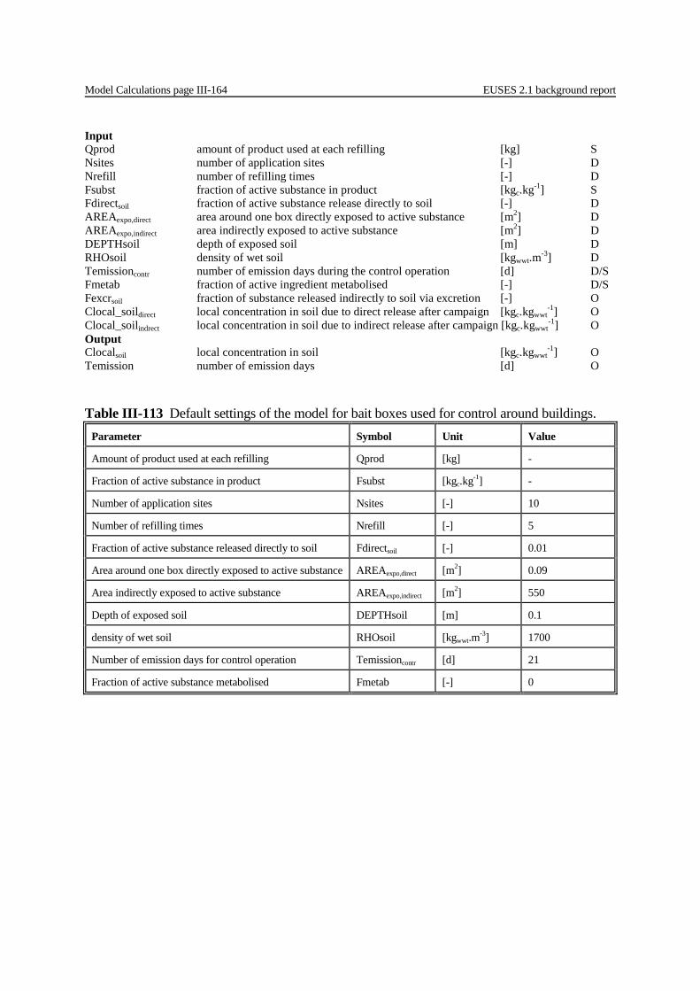
Model Calculations page III-164 EUSES 2.1 background report
Input Qprod amount of product used at each refilling [kg] S Nsites number of application sites [-] D Nrefill number of refilling times [-] D Fsubst fraction of active substance in product [kgc.kg-1] S Fdirectsoil fraction of active substance release directly to soil [-] D AREAexpo,direct area around one box directly exposed to active substance [m2] D AREAexpo,indirect area indirectly exposed to active substance [m2] D DEPTHsoil depth of exposed soil [m] D RHOsoil density of wet soil [kgwwt.m-3] D Temissioncontr number of emission days during the control operation [d] D/S Fmetab fraction of active ingredient metabolised [-] D/S Fexcrsoil fraction of substance released indirectly to soil via excretion [-] O Clocal_soildirect local concentration in soil due to direct release after campaign [kgc.kgwwt
-1] O Clocal_soilindrect local concentration in soil due to indirect release after campaign [kgc.kgwwt
-1] O Output Clocalsoil local concentration in soil [kgc.kgwwt
-1] O Temission number of emission days [d] O
Table III-113 Default settings of the model for bait boxes used for control around buildings. Parameter Symbol Unit Value
Amount of product used at each refilling Qprod [kg] -
Fraction of active substance in product Fsubst [kgc.kg-1] -
Number of application sites Nsites [-] 10
Number of refilling times Nrefill [-] 5
Fraction of active substance released directly to soil Fdirectsoil [-] 0.01
Area around one box directly exposed to active substance AREAexpo,direct [m2] 0.09
Area indirectly exposed to active substance AREAexpo,indirect [m2] 550
Depth of exposed soil DEPTHsoil [m] 0.1
density of wet soil RHOsoil [kgwwt.m-3] 1700
Number of emission days for control operation Temissioncontr [d] 21
Fraction of active substance metabolised Fmetab [-] 0
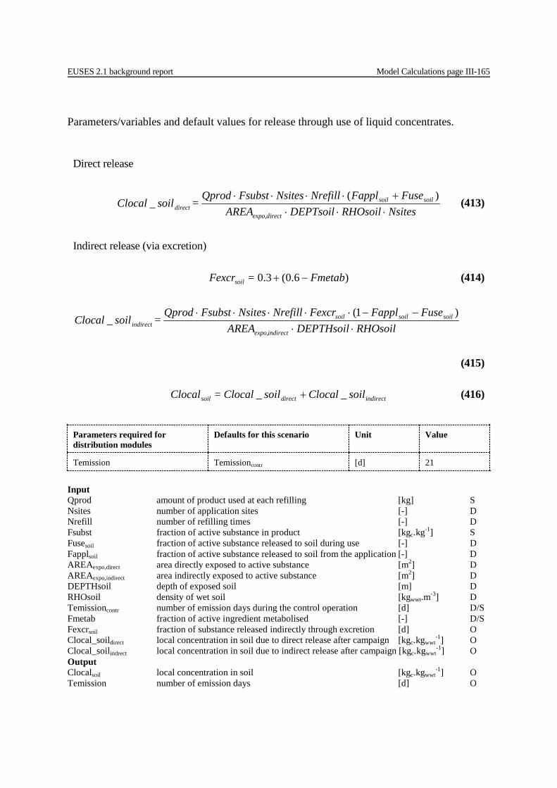
EUSES 2.1 background report Model Calculations page III-165
Parameters/variables and default values for release through use of liquid concentrates.
Parameters required for distribution modules
Defaults for this scenario Unit Value
Temission Temissioncontr [d] 21
Input Qprod amount of product used at each refilling [kg] S Nsites number of application sites [-] D Nrefill number of refilling times [-] D Fsubst fraction of active substance in product [kgc.kg-1] S Fusesoil fraction of active substance released to soil during use [-] D Fapplsoil fraction of active substance released to soil from the application [-] D AREAexpo,direct area directly exposed to active substance [m2] D AREAexpo,indirect area indirectly exposed to active substance [m2] D DEPTHsoil depth of exposed soil [m] D RHOsoil density of wet soil [kgwwt.m-3] D Temissioncontr number of emission days during the control operation [d] D/S Fmetab fraction of active ingredient metabolised [-] D/S Fexcrsoil fraction of substance released indirectly through excretion [d] O Clocal_soildirect local concentration in soil due to direct release after campaign [kgc.kgwwt
-1] O Clocal_soilindrect local concentration in soil due to indirect release after campaign [kgc.kgwwt
-1] O Output Clocalsoil local concentration in soil [kgc.kgwwt
-1] O Temission number of emission days [d] O
Direct release
NsitesRHOsoilDEPTsoilAREA
FuseFapplNrefillNsites Fsubst Qprod = soilClocal
directexpo,
soilsoildirect ⋅⋅⋅
+⋅⋅⋅⋅ )(_ (413)
Indirect release (via excretion)
)6.0(3.0 Fmetab= Fexcrsoil −+ (414)
RHOsoilDEPTHsoilAREAFuseFapplFexcrNrefillNsites Fsubst Qprod
= soilClocalindirectexpo,
soilsoilsoilindirect ⋅⋅
−−⋅⋅⋅⋅⋅ )1(_
(415)
indirectdirectsoil soilClocalsoilClocal= Clocal __ + (416)

Model Calculations page III-166 EUSES 2.1 background report
III.3.6.12.3 Products used for control in open areas Parameters/variables and default values for release through use of pellets and impregnated grain.
Parameters required for distribution modules
Defaults for this scenario Unit Value
Temission Temissioncontr [d] 6
Table III-114 Default settings of the model for the use of liquid concentrates in control around buildings.
Parameter Symbol Unit Value
Amount of product used at each refilling Qprod [kg] -
Fraction of active substance in product Fsubst [kgc.kg-1] -
Number of application sites Nsites [-] 10
Number of refilling times Nrefill [-] 5
Fraction of active substance released to soil during use Fusesoil [-] 0.10
Fraction of active substance release to soil during application
Fapplsoil [-] 0.05
Area directly exposed to active substance AREAexpo,direct [m2] 0.0314
Area indirectly exposed to active substance AREAexpo,indirect [m2] 550
Depth of exposed soil DEPTHsoil [m] 0.1
density of wet soil RHOsoil [kgwwt.m-3] 1700
Number of emission days for control operation Temissioncontr [d] 21
Fraction of active substance metabolised Fmetab [-] 0
2
)( 22 l rR = Vsoil⋅⋅− π (417)
RHOsoilVsoil
FuseFapplNrefillNsites Fsubst Qprod = Clocal soilsoil
soil ⋅+⋅⋅⋅⋅ )( (418)
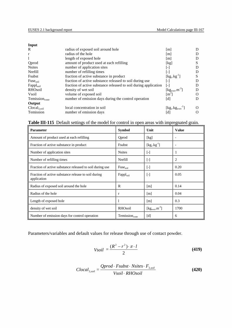
EUSES 2.1 background report Model Calculations page III-167
Input R radius of exposed soil around hole [m] D r radius of the hole [m] D l length of exposed hole [m] D Qprod amount of product used at each refilling [kg] S Nsites number of application sites [-] D Nrefill number of refilling times [-] D Fsubst fraction of active substance in product [kgc.kg-1] S Fusesoil fraction of active substance released to soil during use [-] D Fapplsoil fraction of active substance released to soil during application [-] D RHOsoil density of wet soil [kgwwt.m-3] D Vsoil volume of exposed soil [m3] O Temissioncontr number of emission days during the control operation [d] D Output Clocal3,soil local concentration in soil [kgc.kgwwt
-1] O Temission number of emission days [d] O
Parameters/variables and default values for release through use of contact powder.
Table III-115 Default settings of the model for control in open areas with impregnated grain. Parameter Symbol Unit Value
Amount of product used at each refilling Qprod [kg] -
Fraction of active substance in product Fsubst [kgc.kg-1] -
Number of application sites Nsites [-] 1
Number of refilling times Nrefill [-] 2
Fraction of active substance released to soil during use Fusesoil [-] 0.20
Fraction of active substance release to soil during application
Fapplsoil [-] 0.05
Radius of exposed soil around the hole R [m] 0.14
Radius of the hole r [m] 0.04
Length of exposed hole l [m] 0.3
density of wet soil RHOsoil [kgwwt.m-3] 1700
Number of emission days for control operation Temissioncontr [d] 6
2
)( 22 l rR = Vsoil⋅⋅− π (419)
RHOsoilVsoil
FNsites Fsubst Qprod = Clocal soil
soil ⋅
⋅⋅⋅ ,3,3 (420)
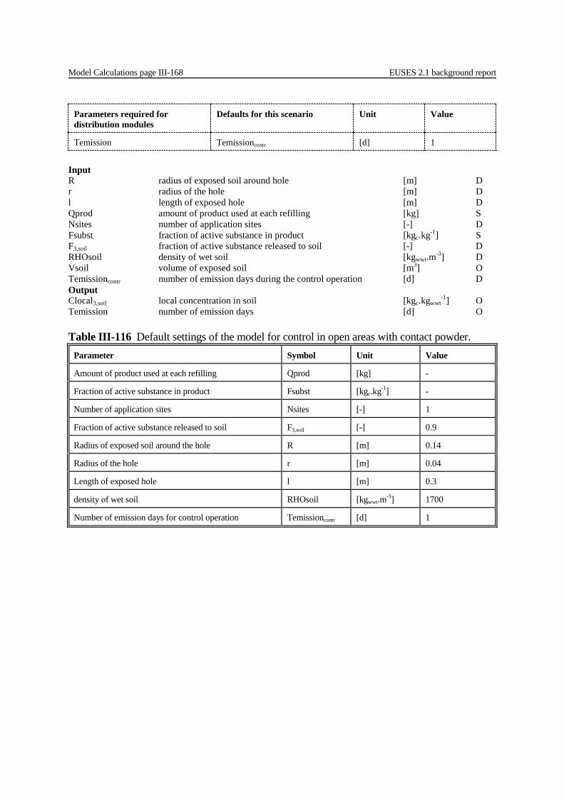
Model Calculations page III-168 EUSES 2.1 background report
Parameters required for distribution modules
Defaults for this scenario Unit Value
Temission Temissioncontr [d] 1
Input R radius of exposed soil around hole [m] D r radius of the hole [m] D l length of exposed hole [m] D Qprod amount of product used at each refilling [kg] S Nsites number of application sites [-] D Fsubst fraction of active substance in product [kgc.kg-1] S F3,soil fraction of active substance released to soil [-] D RHOsoil density of wet soil [kgwwt.m-3] D Vsoil volume of exposed soil [m3] O Temissioncontr number of emission days during the control operation [d] D Output Clocal3,soil local concentration in soil [kgc.kgwwt
-1] O Temission number of emission days [d] O
Table III-116 Default settings of the model for control in open areas with contact powder. Parameter Symbol Unit Value
Amount of product used at each refilling Qprod [kg] -
Fraction of active substance in product Fsubst [kgc.kg-1] -
Number of application sites Nsites [-] 1
Fraction of active substance released to soil F3,soil [-] 0.9
Radius of exposed soil around the hole R [m] 0.14
Radius of the hole r [m] 0.04
Length of exposed hole l [m] 0.3
density of wet soil RHOsoil [kgwwt.m-3] 1700
Number of emission days for control operation Temissioncontr [d] 1

EUSES 2.1 background report Model Calculations page III-169
Parameters/variables and default values for release through gassing.
Parameters required for distribution modules
Defaults for this scenario Unit Value
Temission Temissioncontr [d] 1
Input - type of product used [-] P R radius of exposed soil around hole [m] D r radius of the hole [m] D l length of exposed hole [m] D Qprod amount of product used per 2 ha in control operation [kg] S AREAcontr area treated at control operation [m2] D DOSEprod amount of product used per unit of treated area [kg.m-2] O Nappl number of applications [-] D Fsubst fraction of substance in product [kgc.kg-1] S Fformed fraction of phosphine formed [-] Oc
F3,soil fraction of active substance released to soil [-] D RHOsoil density of wet soil [kgwwt.m-3] D Vsoil volume of exposed soil per treated area (2 ha) [m3] O HEIGHTair atmospheric mixing height [m] D Estdfield,air,24h 24 hour average source strength [-] D Temissioncont number of emission days during the control operation [d] D Output Clocal3,soil local concentration in soil from an application [kgc.kgwwt
-1] O Clocal3,air local concentration in air from an application [kgc.m-3] O Temission number of emission days [d] O
l rR = Vsoil ⋅⋅− π)( 22 (421)
RHOsoilVsoil
FNapplFformed Fsubst Qprod = Clocal soil
soil ⋅⋅
⋅⋅⋅⋅ ,3 (422)
contrAREA
Qprod = DOSEprod (423)
HEIGHTair
EstdFFformed Fsubst DOSEprod = Clocal hairfieldsoil
air24,,,3 )1( ⋅−⋅⋅⋅
(424)
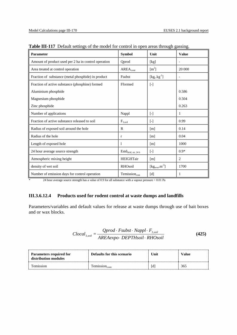
Model Calculations page III-170 EUSES 2.1 background report
* 24 hour average source strength has a value of 0.9 for all substance with a vapour pressure > 0.01 Pa III.3.6.12.4 Products used for rodent control at waste dumps and landfills Parameters/variables and default values for release at waste dumps through use of bait boxes and or wax blocks.
Parameters required for distribution modules
Defaults for this scenario Unit Value
Temission Temissioncontr [d] 365
Table III-117 Default settings of the model for control in open areas through gassing. Parameter Symbol Unit Value
Amount of product used per 2 ha in control operation Qprod [kg] -
Area treated at control operation AREAcontr [m2] 20 000
Fraction of substance (metal phosphide) in product Fsubst [kgc.kg-1] -
Fraction of active substance (phosphine) formed
Aluminium phosphide
Magnesium phosphide
Zinc phosphide
Fformed [-]
0.586
0.504
0.263
Number of applications Nappl [-] 1
Fraction of active substance released to soil F3,soil [-] 0.99
Radius of exposed soil around the hole R [m] 0.14
Radius of the hole r [m] 0.04
Length of exposed hole l [m] 1000
24 hour average source strength Estdfield, air, 24 h [-] 0.9*
Atmospheric mixing height HEIGHTair [m] 2
density of wet soil RHOsoil [kgwwt.m-3] 1700
Number of emission days for control operation Temissioncont [d] 1
RHOsoilDEPTHsoilexpoAREAFNappl Fsubst Qprod
= Clocal soilsoil ⋅⋅
⋅⋅⋅ ,3,3 (425)
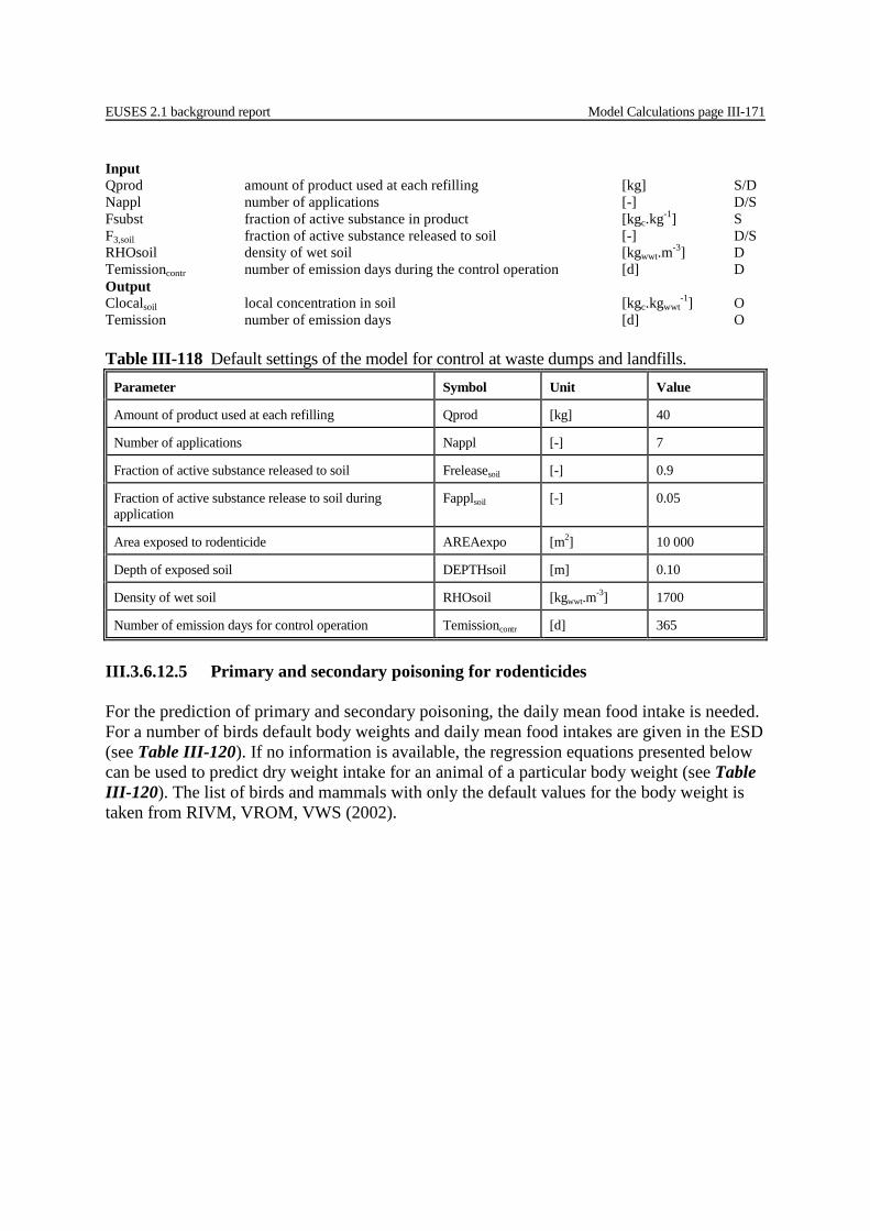
EUSES 2.1 background report Model Calculations page III-171
Input Qprod amount of product used at each refilling [kg] S/D Nappl number of applications [-] D/S Fsubst fraction of active substance in product [kgc.kg-1] S F3,soil fraction of active substance released to soil [-] D/S RHOsoil density of wet soil [kgwwt.m-3] D Temissioncontr number of emission days during the control operation [d] D Output Clocalsoil local concentration in soil [kgc.kgwwt
-1] O Temission number of emission days [d] O
III.3.6.12.5 Primary and secondary poisoning for rodenticides For the prediction of primary and secondary poisoning, the daily mean food intake is needed. For a number of birds default body weights and daily mean food intakes are given in the ESD (see Table III-120). If no information is available, the regression equations presented below can be used to predict dry weight intake for an animal of a particular body weight (see Table III-120). The list of birds and mammals with only the default values for the body weight is taken from RIVM, VROM, VWS (2002).
Table III-118 Default settings of the model for control at waste dumps and landfills. Parameter Symbol Unit Value
Amount of product used at each refilling Qprod [kg] 40
Number of applications Nappl [-] 7
Fraction of active substance released to soil Freleasesoil [-] 0.9
Fraction of active substance release to soil during application
Fapplsoil [-] 0.05
Area exposed to rodenticide AREAexpo [m2] 10 000
Depth of exposed soil DEPTHsoil [m] 0.10
Density of wet soil RHOsoil [kgwwt.m-3] 1700
Number of emission days for control operation Temissioncontr [d] 365
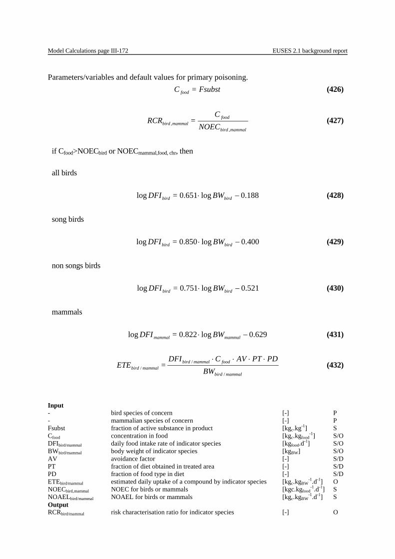
Model Calculations page III-172 EUSES 2.1 background report
Parameters/variables and default values for primary poisoning.
Input - bird species of concern [-] P - mammalian species of concern [-] P Fsubst fraction of active substance in product [kgc.kg-1] S Cfood concentration in food [kgc.kgfood
-1] S/O DFIbird/mammal daily food intake rate of indicator species [kgfood.d-1] S/O BWbird/mammal body weight of indicator species [kgBW] S/O AV avoidance factor [-] S/D PT fraction of diet obtained in treated area [-] S/D PD fraction of food type in diet [-] S/D ETEbird/mammal estimated daily uptake of a compound by indicator species [kgc.kgBW
-1.d-1] O NOECbird,mammal NOEC for birds or mammals [kgc.kgfood
-1.d-1] S NOAELbird/mammal NOAEL for birds or mammals [kgc.kgBW
-1.d-1] S Output RCRbird/mammal risk characterisation ratio for indicator species [-] O
Fsubst= C food (426)
mammalbird
foodmammalbird NOEC
C= RCR
,, (427)
if Cfood>NOECbird or NOECmammal,food, chr, then
all birds
188.0log651.0log −⋅ birdbird BW= DFI (428)
song birds
400.0log850.0log −⋅ birdbird BW= DFI (429)
non songs birds
521.0log751.0log −⋅ birdbird BW= DFI (430)
mammals
629.0log822.0log −⋅ mammalmammal BW= DFI (431)
mammalbird
foodmammalbirdmammalbird BW
PDPTAV C DFI = ETE
/
//
⋅⋅⋅⋅ (432)
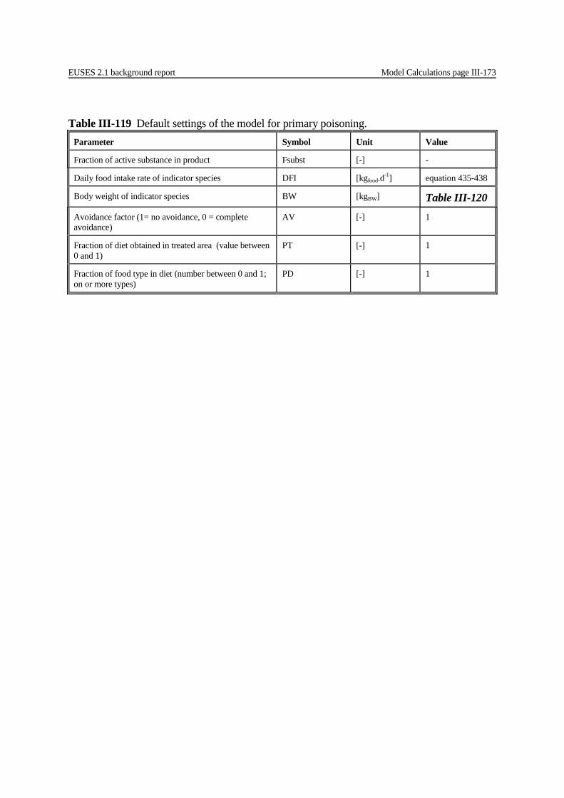
EUSES 2.1 background report Model Calculations page III-173
Table III-119 Default settings of the model for primary poisoning. Parameter Symbol Unit Value
Fraction of active substance in product Fsubst [-] -
Daily food intake rate of indicator species DFI [kgfood.d-1] equation 435-438
Body weight of indicator species BW [kgBW] Table III-120
Avoidance factor (1= no avoidance, 0 = complete avoidance)
AV [-] 1
Fraction of diet obtained in treated area (value between 0 and 1)
PT [-] 1
Fraction of food type in diet (number between 0 and 1; on or more types)
PD [-] 1
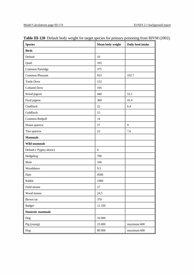
Model Calculations page III-174 EUSES 2.1 background report
Table III-120 Default body weight for target species for primary poisoning from RIVM (2002). Species Mean body weight Daily food intake
Birds
Default 10
Quail 102
Common Partridge 375
Common Pheasant 953 102.7
Turtle Dove 152
Collared Dove 195
Wood pigeon 440 53.1
Feral pigeon 360 41.4
Chaffinch 22 6.4
Goldfinch 15
Common Redpoll 14
House sparrow 27 9
Tree sparrow 22 7.6
Mammals
Wild mammals
Default ( Pygmy shrew) 6
Hedgehog 700
Mole 100
Woodshrew 9.5
Hare 4500
Rabbit 1900
Field mouse 27
Wood mouse 24.5
Brown rat 370
Badger 11 250
Domestic mammals
Dog 10 000
Pig (young) 25 000 maximum 600
Hog 80 000 maximum 600
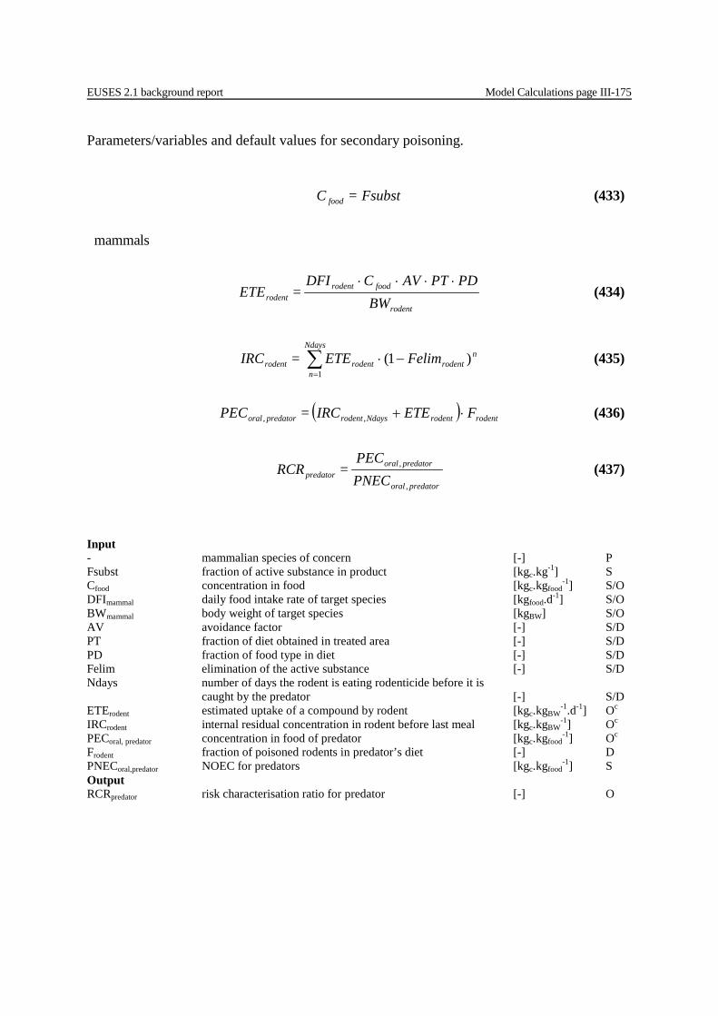
EUSES 2.1 background report Model Calculations page III-175
Parameters/variables and default values for secondary poisoning.
Input - mammalian species of concern [-] P Fsubst fraction of active substance in product [kgc.kg-1] S Cfood concentration in food [kgc.kgfood
-1] S/O DFImammal daily food intake rate of target species [kgfood.d-1] S/O BWmammal body weight of target species [kgBW] S/O AV avoidance factor [-] S/D PT fraction of diet obtained in treated area [-] S/D PD fraction of food type in diet [-] S/D Felim elimination of the active substance [-] S/D Ndays number of days the rodent is eating rodenticide before it is caught by the predator [-] S/D ETErodent estimated uptake of a compound by rodent [kgc.kgBW
-1.d-1] Oc
IRCrodent internal residual concentration in rodent before last meal [kgc.kgBW-1] Oc
PECoral, predator concentration in food of predator [kgc.kgfood-1] Oc
Frodent fraction of poisoned rodents in predator’s diet [-] D PNECoral,predator NOEC for predators [kgc.kgfood
-1] S Output RCRpredator risk characterisation ratio for predator [-] O
Fsubst= C food (433)
mammals
rodent
foodrodentrodent BW
PDPTAV C DFI = ETE
⋅⋅⋅⋅ (434)
∑=
−⋅Ndays
n
nrodentrodentrodent elimFETE= IRC
1)1( (435)
( ) rodentrodentNdaysrodentpredatororal FETEIRC = PEC ⋅+,, (436)
predatororal
predatororalpredator PNEC
PEC = RCR
,
, (437)
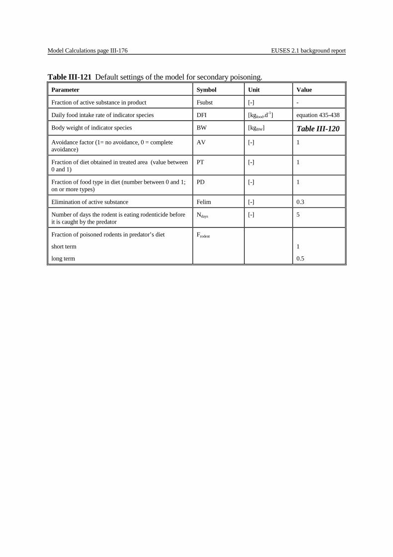
Model Calculations page III-176 EUSES 2.1 background report
Table III-121 Default settings of the model for secondary poisoning. Parameter Symbol Unit Value
Fraction of active substance in product Fsubst [-] -
Daily food intake rate of indicator species DFI [kgfood.d-1] equation 435-438
Body weight of indicator species BW [kgBW] Table III-120
Avoidance factor (1= no avoidance, 0 = complete avoidance)
AV [-] 1
Fraction of diet obtained in treated area (value between 0 and 1)
PT [-] 1
Fraction of food type in diet (number between 0 and 1; on or more types)
PD [-] 1
Elimination of active substance Felim [-] 0.3
Number of days the rodent is eating rodenticide before it is caught by the predator
Ndays [-] 5
Fraction of poisoned rodents in predator’s diet
short term
long term
Frodent
1
0.5
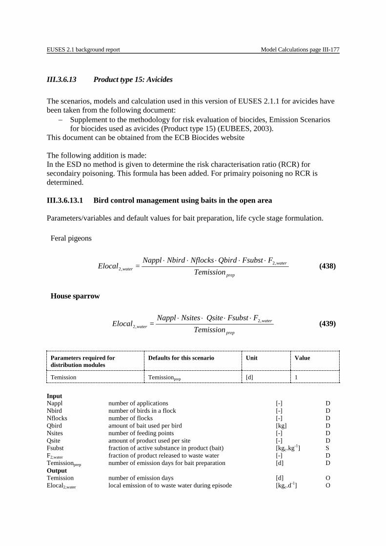
EUSES 2.1 background report Model Calculations page III-177
III.3.6.13 Product type 15: Avicides The scenarios, models and calculation used in this version of EUSES 2.1.1 for avicides have been taken from the following document:
− Supplement to the methodology for risk evaluation of biocides, Emission Scenarios for biocides used as avicides (Product type 15) (EUBEES, 2003).
This document can be obtained from the ECB Biocides website The following addition is made: In the ESD no method is given to determine the risk characterisation ratio (RCR) for secondairy poisoning. This formula has been added. For primairy poisoning no RCR is determined. III.3.6.13.1 Bird control management using baits in the open area Parameters/variables and default values for bait preparation, life cycle stage formulation.
Parameters required for distribution modules
Defaults for this scenario Unit Value
Temission Temissionprep [d] 1
Input Nappl number of applications [-] D Nbird number of birds in a flock [-] D Nflocks number of flocks [-] D Qbird amount of bait used per bird [kg] D Nsites number of feeding points [-] D Qsite amount of product used per site [-] D Fsubst fraction of active substance in product (bait) [kgc.kg-1] S F2,water fraction of product released to waste water [-] D Temissionprep number of emission days for bait preparation [d] D Output Temission number of emission days [d] O Elocal2,water local emission of to waste water during episode [kgc.d-1] O
Feral pigeons
prep
waterwater Temission
FFsubstQbird Nflocks NbirdNappl = Elocal ,2
,2
⋅⋅⋅⋅⋅ (438)
House sparrow
prep
waterwater Temission
FFsubstQsite NsitesNappl = Elocal ,2
,2
⋅⋅⋅⋅ (439)
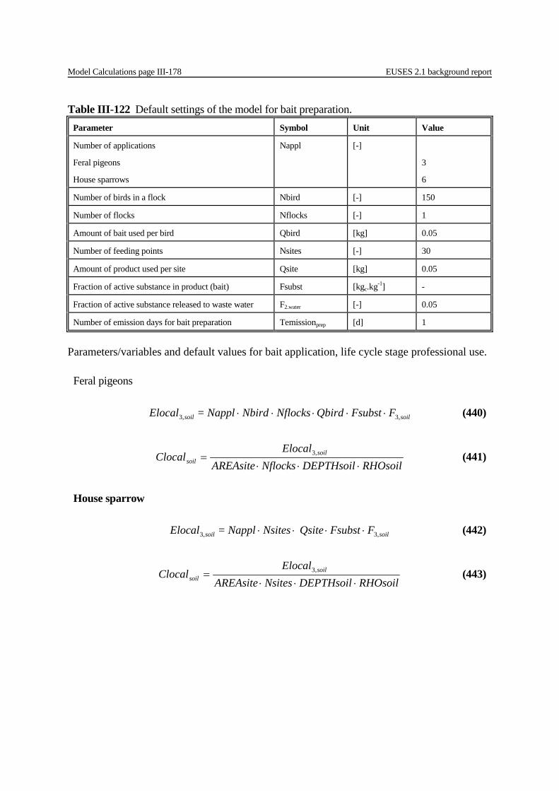
Model Calculations page III-178 EUSES 2.1 background report
Parameters/variables and default values for bait application, life cycle stage professional use.
Table III-122 Default settings of the model for bait preparation. Parameter Symbol Unit Value
Number of applications
Feral pigeons
House sparrows
Nappl [-]
3
6
Number of birds in a flock Nbird [-] 150
Number of flocks Nflocks [-] 1
Amount of bait used per bird Qbird [kg] 0.05
Number of feeding points Nsites [-] 30
Amount of product used per site Qsite [kg] 0.05
Fraction of active substance in product (bait) Fsubst [kgc.kg-1] -
Fraction of active substance released to waste water F2.water [-] 0.05
Number of emission days for bait preparation Temissionprep [d] 1
Feral pigeons
soilsoil FFsubstQbird Nflocks NbirdNappl = Elocal ,3,3 ⋅⋅⋅⋅⋅ (440)
RHOsoilDEPTHsoilNflocksAREAsite
ElocalClocal soil
soil ⋅⋅⋅= ,3 (441)
House sparrow
soilsoil FFsubstQsite NsitesNappl = Elocal ,3,3 ⋅⋅⋅⋅ (442)
RHOsoilDEPTHsoilNsitesAREAsite
ElocalClocal soil
soil ⋅⋅⋅= ,3 (443)
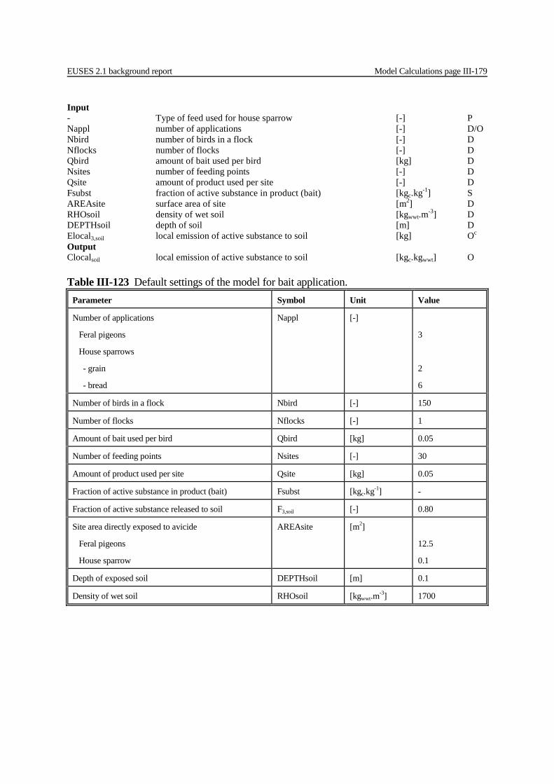
EUSES 2.1 background report Model Calculations page III-179
Input - Type of feed used for house sparrow [-] P Nappl number of applications [-] D/O Nbird number of birds in a flock [-] D Nflocks number of flocks [-] D Qbird amount of bait used per bird [kg] D Nsites number of feeding points [-] D Qsite amount of product used per site [-] D Fsubst fraction of active substance in product (bait) [kgc.kg-1] S AREAsite surface area of site [m2] D RHOsoil density of wet soil [kgwwt.m-3] D DEPTHsoil depth of soil [m] D Elocal3,soil local emission of active substance to soil [kg] Oc
Output Clocalsoil local emission of active substance to soil [kgc.kgwwt] O
Table III-123 Default settings of the model for bait application. Parameter Symbol Unit Value
Number of applications
Feral pigeons
House sparrows
- grain
- bread
Nappl [-]
3
2
6
Number of birds in a flock Nbird [-] 150
Number of flocks Nflocks [-] 1
Amount of bait used per bird Qbird [kg] 0.05
Number of feeding points Nsites [-] 30
Amount of product used per site Qsite [kg] 0.05
Fraction of active substance in product (bait) Fsubst [kgc.kg-1] -
Fraction of active substance released to soil F3,soil [-] 0.80
Site area directly exposed to avicide
Feral pigeons
House sparrow
AREAsite [m2]
12.5
0.1
Depth of exposed soil DEPTHsoil [m] 0.1
Density of wet soil RHOsoil [kgwwt.m-3] 1700

Model Calculations page III-180 EUSES 2.1 background report
III.3.6.13.2 Bird control management in the open area using egg-oil coating Parameters/variables and default values for application of egg-oil coating.
Input - type of application [-] P Nnest number of nests to be treated at one site [-] D Negg number of eggs per nest [-] D Nappl number of applications [-] D Vformegg amount of product needed to cover one egg completely [m3] D Fsubst fraction of active substance in product [kgc.kg-1] S RHOform density of product [kg.m-3] S F3.soil fraction of product lost during application [-] O AREAsoil surface area near nest [m2] D RHOsoil density of wet soil [kgwwt.m-3] D DEPTHsoil depth of soil [m] D Elocal3,soil local emission of active substance to soil during campaign [kg] Oc
Output Clocalsoil local concentration of active substance in soil [kgc.kgwwt] O
soileggsoil FNapplFsubstRHOform Vform NeggsNnest = Elocal ,3,3 ⋅⋅⋅⋅⋅⋅ (444)
RHOsoilDEPTHsoilNapplNnestAREAsoil
ElocalClocal soil
soil ⋅⋅⋅⋅= ,3 (445)
Table III-124 Default settings of the model for egg-oil application. Parameter Symbol Unit Value
Number of nests to be treated at one site Nnest [-] 150
Number of eggs per nest Negg [-] 6
Number of applications Nappl [-] 1
Volume of product needed to cover one egg completely Vformegg [m3] 7.10-6
Fraction of active substance in product Fsubst [kgc.kg-1] -
Fraction of active substance released to soil
spraying
immersion
F3.soil [-]
0.1
0.0
Density of product RHOform [kgwwt.m-3] -
Exposed area near nest (nest+surrounding surface) AREAsoil [m2] 0.33
Depth of exposed soil DEPTHsoil [m] 0.1
Density of wet soil RHOsoil [kg.m-3] 1700

EUSES 2.1 background report Model Calculations page III-181
Parameters/variables and default values for release of egg-oil during service life (life cycle stage 5).
Input - type of application [-] P Negg number of eggs per nest [-] D Nappl number of applications [-] D Vformegg amount of product needed to cover one egg completely [m3] D Fsubst fraction of active substance in product [kgc.kg-1] S RHOform density of product [kg.m-3] S F3.soil fraction of product lost to soil during application [-] O Fdrift fraction of product lost during application due to spray-drift [-] D Nrain number of rain events [-] D Fleach fraction of product lost during application due to spray-drift [-] D Qleach quantity of active substance on egg just after the application [kg] O Elocal5,soil local emission of active substance to soil due to leaching [-] Oc
AREAsoil surface area near nest [m2] D RHOsoil density of wet soil [kgwwt.m-3] D DEPTHsoil depth of soil [m] D Clocalappl,soil local concentration in soil due to application (stage 3) [kgc.kgwwt
-1] Oc
Output Clocalsoil total local emission of active substance to soil [kgc.kgwwt
-1] O
)1( ,3 FdriftFNapplFsubstRHOform Vform Neggs = Qleach soilegg −−⋅⋅⋅⋅⋅ (446)
∑=
−−⋅⋅Nrain
i
Nrainsoil FleachFleachQleach = Elocal
1
1,5 )1( (447)
soilapplsoil
soil ClocalRHOsoilDEPTHsoilNapplAREAsoil
ElocalClocal ,
,5 +⋅⋅⋅
= (448)
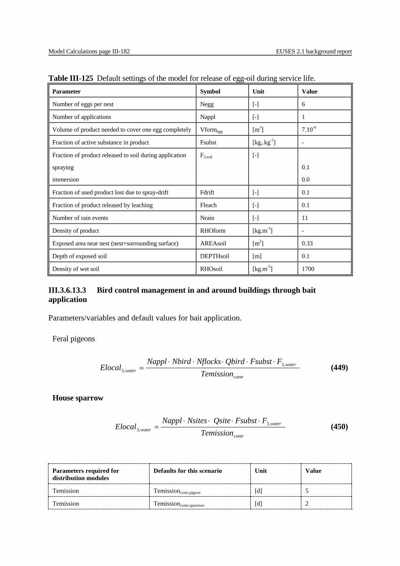
Model Calculations page III-182 EUSES 2.1 background report
III.3.6.13.3 Bird control management in and around buildings through bait application Parameters/variables and default values for bait application.
Parameters required for distribution modules
Defaults for this scenario Unit Value
Temission Temissioncontr,pigeon [d] 5
Temission Temissioncontr,sparrouw [d] 2
Table III-125 Default settings of the model for release of egg-oil during service life. Parameter Symbol Unit Value
Number of eggs per nest Negg [-] 6
Number of applications Nappl [-] 1
Volume of product needed to cover one egg completely Vformegg [m3] 7.10-6
Fraction of active substance in product Fsubst [kgc.kg-1] -
Fraction of product released to soil during application
spraying
immersion
F3.soil [-]
0.1
0.0
Fraction of used product lost due to spray-drift Fdrift [-] 0.1
Fraction of product released by leaching Fleach [-] 0.1
Number of rain events Nrain [-] 11
Density of product RHOform [kg.m-3] -
Exposed area near nest (nest+surrounding surface) AREAsoil [m2] 0.33
Depth of exposed soil DEPTHsoil [m] 0.1
Density of wet soil RHOsoil [kg.m-3] 1700
Feral pigeons
contr
waterwater Temission
FFsubstQbird Nflocks NbirdNapplElocal ,3
,3
⋅⋅⋅⋅⋅= (449)
House sparrow
contr
waterwater Temission
FFsubstQsite NsitesNapplElocal ,3
,3
⋅⋅⋅⋅= (450)
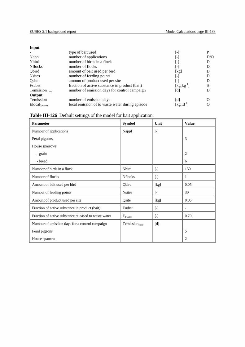
EUSES 2.1 background report Model Calculations page III-183
Input - type of bait used [-] P Nappl number of applications [-] D/O Nbird number of birds in a flock [-] D Nflocks number of flocks [-] D Qbird amount of bait used per bird [kg] D Nsites number of feeding points [-] D Qsite amount of product used per site [-] D Fsubst fraction of active substance in product (bait) [kgckg-1] S Temissioncontr number of emission days for control campaign [d] D Output Temission number of emission days [d] O Elocal3,water local emission of to waste water during episode [kgc.d-1] O
Table III-126 Default settings of the model for bait application. Parameter Symbol Unit Value
Number of applications
Feral pigeons
House sparrows
- grain
- bread
Nappl [-]
3
2
6
Number of birds in a flock Nbird [-] 150
Number of flocks Nflocks [-] 1
Amount of bait used per bird Qbird [kg] 0.05
Number of feeding points Nsites [-] 30
Amount of product used per site Qsite [kg] 0.05
Fraction of active substance in product (bait) Fsubst [-] -
Fraction of active substance released to waste water F3.water [-] 0.70
Number of emission days for a control campaign
Feral pigeons
House sparrow
Temissioncontr
[d]
5
2

Model Calculations page III-184 EUSES 2.1 background report
III.3.6.13.4 Bird control management in and around buildings using egg-oil coating Parameters/variables and default values for application of egg-oil coating.
Parameters required for distribution modules
Defaults for this scenario Unit Value
Temission Temissionleach [d] 1
Input - controlled species [-] P Nsites number of application sites [-] D Nnest number of nests to be treated at one site [-] D Negg number of eggs per nest [-] D Nappl number of applications [-] D Vformegg amount of product needed to cover one egg completely [m3] D Fsubst fraction of active substance in product [kgc.kg] S RHOform density of product [kg.m-3] S Fdrift fraction of product lost during application [-] D Fleach fraction of product lost due to leaching after rain event [-] D Quse amount of substance used for eggs-coating [kgc] O Elocaldrift local emission of active substance to water due to drift [-] O Elocaldrift local emission of active substance to water due to leaching [-] O Temissionleach number of emission days for leaching at the stage of service life [d] D Temissionappl number of emission days for the stage of application [d] D Output Temission number of emission days [-] O Elocal3,water local emission of active substance to waste water [kgc.d-1] O
NapplFsubstRHOform Vform NeggsNnestNsites = Quse egg ⋅⋅⋅⋅⋅⋅ (451)
appldrift Temission
FdriftQuse = Elocal ⋅
(452)
leach
leach TemissionFleachFdriftQuse = Elocal ⋅−⋅ )1( (453)
leachdriftwater ElocalElocal = Elocal +,3 (454)

EUSES 2.1 background report Model Calculations page III-185
III.3.6.13.5 Primary and secondary poisoning for avicides For the prediction of primary and secondary poisoning, the daily mean food intake is needed. For a number of birds default body weights and daily mean food intakes are given in the ESD (see Table III-120). If no information is available, the regression equations presented below can be used to predict dry weight intake for an animal of a particular body weight (see Table III-120). The list of birds and mammals with only the default values for the body weight is taken from RIVM, VROM, VWS (2002).
Table III-127 Default settings of the model for egg-oil application. Parameter Symbol Unit Value
Number of application sites Nsites [-] 1
Number of nests to be treated at one site Nnest [-] 1000
Number of eggs per nest Negg [-] 3
Number of applications Nappl [-] 1
Volume of product needed to cover one egg completely
Lesser Black-backed Gull
Herring Gull
Great Black-backed Gull
Vformegg [m3]
2.6.10-6
2.9.10-6
3.4.10-6
Fraction of active substance released to waste water due to spraying
Fdrift [-] 0.1
Fraction of active substance released to waste water due to leaching
Fleach [-] 0.1
Density of product RHOform [kg.m-3] -
Number of emission days for the stage of application Temissionappl [d] 2
Number of emission days for the stage of service life Temissionleach [d] 1
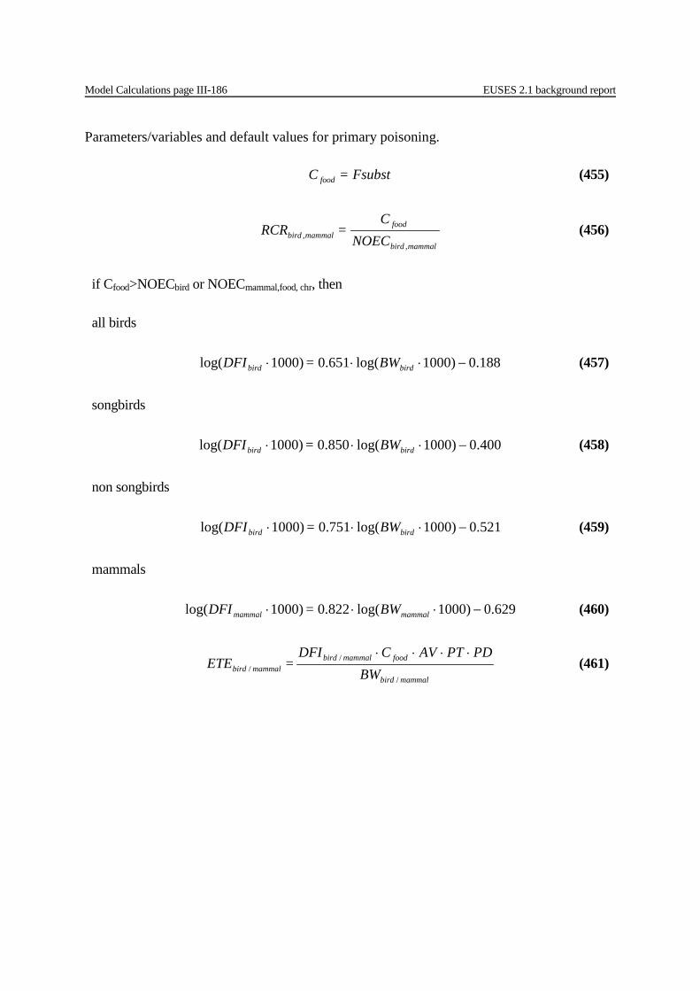
Model Calculations page III-186 EUSES 2.1 background report
Parameters/variables and default values for primary poisoning.
Fsubst= C food (455)
mammalbird
foodmammalbird NOEC
C= RCR
,, (456)
if Cfood>NOECbird or NOECmammal,food, chr, then
all birds
188.0)1000log(651.0)1000log( −⋅⋅⋅ birdbird BW= DFI (457)
songbirds
400.0)1000log(850.0)1000log( −⋅⋅⋅ birdbird BW= DFI (458)
non songbirds
521.0)1000log(751.0)1000log( −⋅⋅⋅ birdbird BW= DFI (459)
mammals
629.0)1000log(822.0)1000log( −⋅⋅⋅ mammalmammal BW= DFI (460)
mammalbird
foodmammalbirdmammalbird BW
PDPTAV C DFI = ETE
/
//
⋅⋅⋅⋅ (461)

EUSES 2.1 background report Model Calculations page III-187
Input - bird species of concern [-] P - mammalian species of concern [-] P Fsubst fraction of active substance in product [-] S Cfood concentration in food [kgc.kgfood
-1] S/O DFIbird/mammal daily food intake rate of indicator species [kgfood.d-1] S/O BWbird/mammal body weight of indicator species [kgBW] S/O AV avoidance factor [-] S/D PT fraction of diet obtained in treated area [-] S/D PD fraction of food type in diet [-] S/D ETEbird/mammal estimated daily uptake of a compound by indicator species [kgc.kgBW
-1.d-1] O NOECbird,mammal NOEC for bird or mammal of concern [kgc.kgfood
-1.d-1] S NOAELbird/mammal NOAEL for bird or mammal of concern [kgc.kgBW
-1.d-1] S Output RCRbird/mammal risk characterisation ratio for indicator species [-] O
Table III-128 Default settings of the model for primary poisoning. Parameter Symbol Unit Value
Fraction of active substance in product Fsubst [-] -
Daily food intake rate of indicator species DFI [kgfood.d-1] equation 464-467
Body weight of indicator species BW [kgBW] Table III-120
Avoidance factor (1= no avoidance, 0 = complete avoidance)
bird
mammal
AV [-] xxxxxxxxxxxxxxx
1.0
1.0
Fraction of diet obtained in treated area (value between 0 and 1)
bird
mammal
PT [-] xxxxxxxxxxxxxxx
0.2
1.0
Fraction of food type in diet (number between 0 and 1; on or more types)
bird
mammals
- domestic
- wild
PD [-] xxxxxxxxxxxxxxx
1.0
0.1
0.4
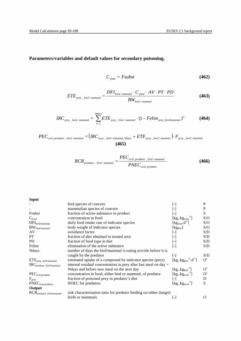
Model Calculations page III-188 EUSES 2.1 background report
Parameters/variables and default values for secondary poisoning.
Input - bird species of concern [-] P - mammalian species of concern [-] P Fsubst fraction of active substance in product [-] S Cfood concentration in food [kgc.kgfood
-1] S/O DFIbird/mammal daily food intake rate of indicator species [kgfood.d-1] S/O BWbird/mammal body weight of indicator species [kgBW] S/O AV avoidance factor [-] S/D PT fraction of diet obtained in treated area [-] S/D PD fraction of food type in diet [-] S/D Felim elimination of the active substance [-] S/D Ndays number of days the bird/mammal is eating avicide before it is caught by the predator [-] S/D ETEprey_bird/mammal estimated uptake of a compound by indicator species (prey) [kgc.kgBW
-1.d-1] Oc
IRCpredator_bird/mammal internal residual concentration in prey after last meal on day = Ndays and before new meal on the next day [kgc.kgBW
-1] Oc
PECoral,predator concentration in food, either bird or mammal, of predator [kgc.kgfood-1] Oc
Fprey fraction of poisoned prey in predator’s diet [-] D PNECoral,predator NOEC for predators [kgc.kgfood
-1] S Output RCRpredator_bird/mammal risk characterisation ratio for predator feeding on either (target) birds or mammals [-] O
Fsubst= C food (462)
mammalbird
foodmammalbirdmammalbirdprey BW
PDPTAV C DFI = ETE
/
//_
⋅⋅⋅⋅ (463)
∑=
−⋅Ndays
n
nmammalprey_bird/mammalbirdpreymammalbirdprey elimFETE= IRC
1/_/_ )1( (464)
( ) mammalbirdpreymammalbirdpreyNdaysmammalbirdpreymammalbirdpredatororal FETEIRC = PEC /_/_,/_/_, ⋅+ (465)
predatororal
mammalbirdpredatororalmammalbirdpredator PNEC
PEC = RCR
,
/_,/_ (466)

EUSES 2.1 background report Model Calculations page III-189
Table III-129 Default settings of the model for secondary poisoning. Parameter Symbol Unit Value
Fraction of active substance in product Fsubst [-] -
Daily food intake rate of indicator species DFI [kgfood.d-1] equation 464-467
Body weight of indicator species BW [kgBW] Table III-120
Avoidance factor (1= no avoidance, 0 = complete avoidance)
AV [-] 1.0
Fraction of diet obtained in treated area (value between 0 and 1)
bird
mammal
PT [-] 1.0
0.2
1.0
Fraction of food type in diet (number between 0 and 1; on or more types)
bird
mammals
- domestic
- wild
PD [-]
1.0
0.1
0.4
Elimination of active substance Felim [-] 0.8
Number of days the rodent is eating rodenticide before it is caught by the predator
pigeon
sparrow
Ndays [-] xxxxxxxxxxxxxxx
5
2
Fraction of poisoned prey in predator’s diet
bird
mammals
Fprey
1.0
0.5
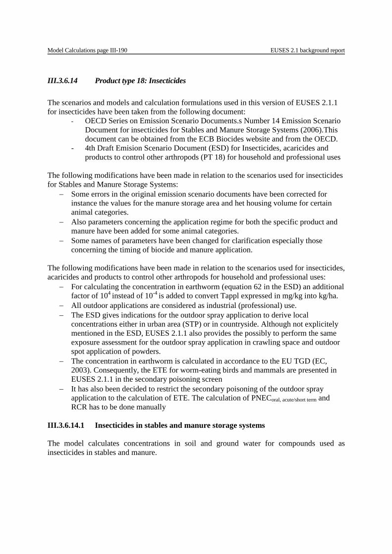
Model Calculations page III-190 EUSES 2.1 background report
III.3.6.14 Product type 18: Insecticides The scenarios and models and calculation formulations used in this version of EUSES 2.1.1 for insecticides have been taken from the following document:
- OECD Series on Emission Scenario Documents.s Number 14 Emission Scenario Document for insecticides for Stables and Manure Storage Systems (2006).This document can be obtained from the ECB Biocides website and from the OECD.
- 4th Draft Emision Scenario Document (ESD) for Insecticides, acaricides and products to control other arthropods (PT 18) for household and professional uses
The following modifications have been made in relation to the scenarios used for insecticides for Stables and Manure Storage Systems:
− Some errors in the original emission scenario documents have been corrected for instance the values for the manure storage area and het housing volume for certain animal categories.
− Also parameters concerning the application regime for both the specific product and manure have been added for some animal categories.
− Some names of parameters have been changed for clarification especially those concerning the timing of biocide and manure application.
The following modifications have been made in relation to the scenarios used for insecticides, acaricides and products to control other arthropods for household and professional uses:
− For calculating the concentration in earthworm (equation 62 in the ESD) an additional factor of 104 instead of 10-4 is added to convert Tappl expressed in mg/kg into kg/ha.
− All outdoor applications are considered as industrial (professional) use. − The ESD gives indications for the outdoor spray application to derive local
concentrations either in urban area (STP) or in countryside. Although not explicitely mentioned in the ESD, EUSES 2.1.1 also provides the possibly to perform the same exposure assessment for the outdoor spray application in crawling space and outdoor spot application of powders.
− The concentration in earthworm is calculated in accordance to the EU TGD (EC, 2003). Consequently, the ETE for worm-eating birds and mammals are presented in EUSES 2.1.1 in the secondary poisoning screen
− It has also been decided to restrict the secondary poisoning of the outdoor spray application to the calculation of ETE. The calculation of PNECoral, acute/short term and RCR has to be done manually
III.3.6.14.1 Insecticides in stables and manure storage systems The model calculates concentrations in soil and ground water for compounds used as insecticides in stables and manure.
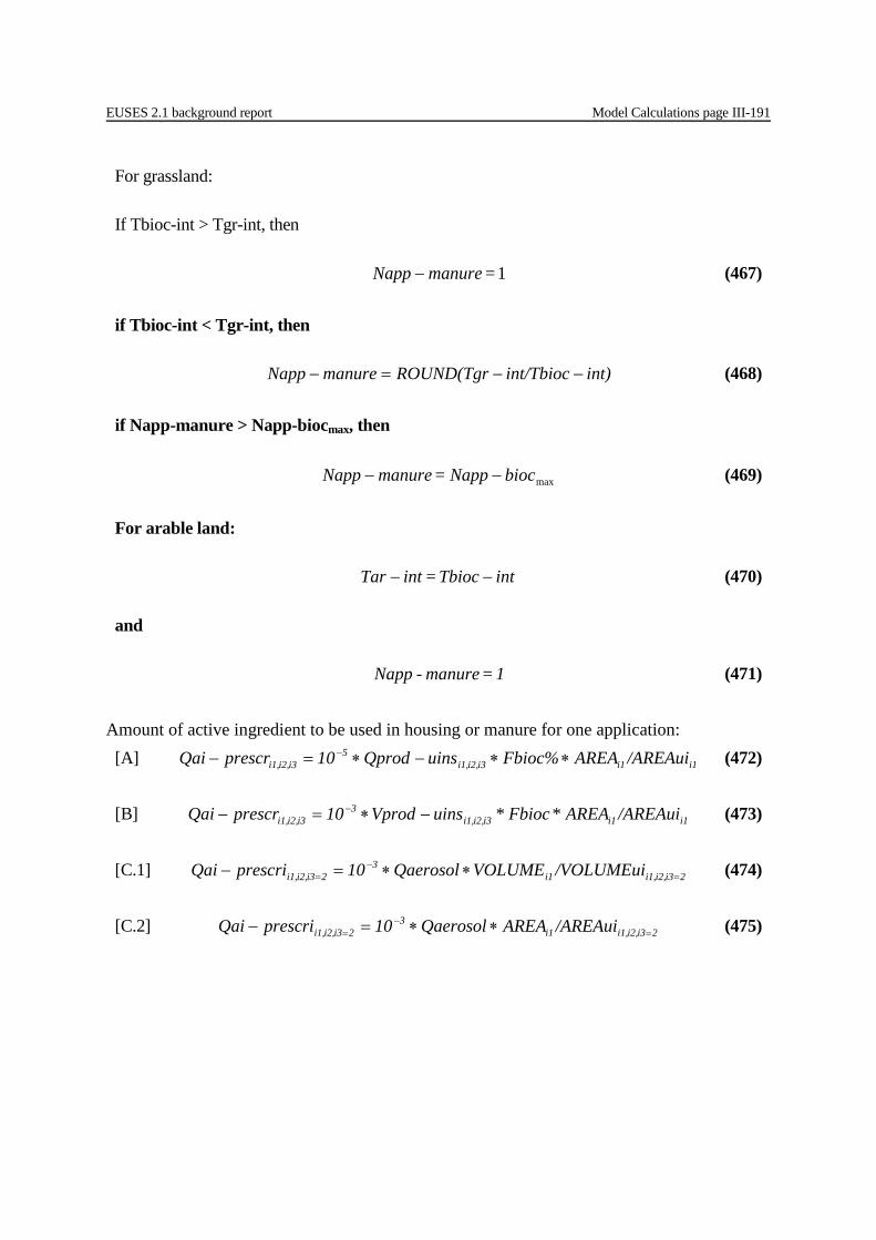
EUSES 2.1 background report Model Calculations page III-191
Amount of active ingredient to be used in housing or manure for one application:
For grassland:
If Tbioc-int > Tgr-int, then
1 = manureNapp − (467)
if Tbioc-int < Tgr-int, then
int)int/TbiocROUND(TgrmanureNapp −−=− (468)
if Napp-manure > Napp-biocmax, then
maxbiocNapp = manureNapp −− (469)
For arable land:
intTbioc = intTar −− (470)
and
1 = manure-Napp (471)
[A] i1i1i3i2,i1,5
i3i2,i1, /AREAuiAREAFbioc%uinsQprod10prescrQai ∗∗−∗=− − (472)
[B] i1i1i3i2,i1,3
i3i2,i1, /AREAuiAREA*Fbioc*uinsVprod10prescrQai −∗=− − (473)
[C.1] 2i3i2,i1,i13
2i3i2,i1, /VOLUMEuiVOLUMEQaerosol10prescriQai =−
= ∗∗=− (474)
[C.2] 2i3i2,i1,i13
2i3i2,i1, /AREAuiAREAQaerosol10prescriQai =−
= ∗∗=− (475)
Model Calculations page III-192 EUSES 2.1 background report
Amount of active ingredient in relevant stream after one application:
[A+B+C] i3i2,i1,i4i3,i2,i1,i4i3,i2,i1, prescr-QaiFQai ∗= (476)
for both application in housings and at manure storage systems, where p is relevant housing category (i1 = 1-18) and q (i1= 19,20) is the relevant storage system:
i4i3,i2,q,i4i3,i2,p,i4i3,i2,tot, QaiQaiQai += (477)
calculating the amount of active ingredient which goes to manure or slurry for
grassland:
gri4i3,i2,i1,i4i3,i2,i1, manureNappQaigrassQai −∗=− (478)
arable land:
ari4i3,i2,i1,i4i3,i2,i1, manure-NappQaiarabQai ∗=− (479)
calculation of the amount of phosphate and nitrogen in manure produced during the relevant period
i2i1i1i4i1, intTar*QphosphNarab-Qphosph −∗= (480)
i2i1i1i4i1, intTgr*QphosphNgrass-Qphosph −∗= (481)
i2i1i1i4i1, int-TarQnitrogNarab-Qnitrog ∗∗= (482)
i2i1i1i4i1, int-TgrQnitrogNgrass-Qnitrog ∗∗= (483)

EUSES 2.1 background report Model Calculations page III-193
Concentration of the active ingredient in soil based on phosphorous or nitrogen immission standards for both grassland and arable land:
wetgrasslandi4i1,
grasslandP2O5,i4i3,i2,i1,i4i3,i2,i1, RHOsoilDEPTHgrassNlappgrass-Qphosph
QgrassQaiP2O5-PIECgrs
∗∗−∗
∗∗−=
−410
(484)
wetdarable_lani4i1,
darable_lanP2O5,i4i3,i2,i1,i4i3,i2,i1, RHOsoilDEPTH*arabNlapparab-Qphosph
QarabQaiP2O5-PIECars
∗−∗
∗∗−=
−410
(485)
wetgrasslandi4i1,
4grasslandN,i4i3,i2,i1,
i4i3,i2,i1, RHOsoilDEPTH*grassNlappgrass-Qnitrog10QgrassQai
N-PIECgrs∗−∗
∗∗−=
−
(486)
wetdarable_lani4i1,
4darable_lanN,i4i3,i2,i1,
i4i3,i2,i1, RHOsoilDEPTHarab-Qnitrog10QarabQai
N-PIECars∗∗−∗
∗∗−=
−
arabNlapp
(487)

Model Calculations page III-194 EUSES 2.1 background report
Concentration of the active ingredient in ground water and surface water:
Based on phosphate immission standards
watersoil
weti4i3,i2,i1,i4i3,i2,i1, K
RHOsoilP2O5-PIECgrsP2O5-gw-PIECgrs
−
−∗∗=
310 (488)
watersoil
weti4i3,i2,i1,i4i3,i2,i1, K
RHOsoilP2O5-PIECarsP2O5-gw-PIECars
−
−∗∗=
310 (489)
offrunwatersoil DILUTIONK −−
−
∗
∗∗=
3weti4i3,i2,i1,
i4i3,i2,i1,
10RHOP2O5-PIECgrsP2O5-water-PIECgrs (490)
offrunwatersoil DILUTONK −−
−
∗
∗∗=
3weti4i3,i2,i1,
i4i3,i2,i1,
10RHOP2O5-PIECarsP2O5-water-PIECars (491)
Based on nitrogen immision standards
watersoil
weti4i3,i2,i1,i4i3,i2,i1, K
RHOsoilN-PIECgrsN-gw-PIECgrs
−
−∗∗=
310 (492)
watersoil
weti4i3,i2,i1,i4i3,i2,i1, K
RHOsoilN-PIECarsN-gw-PIECars
−
−∗∗=
310 (493)
offrunwatersoil DILUTIONK −−
−
∗
∗∗=
3weti4i3,i2,i1,
i4i3,i2,i1,
10RHON-PIECgrsN-water-PIECgrs (494)
offrunwatersoil DILUTIONK −−
−
∗
∗∗=
3weti4i3,i2,i1,
i4i3,i2,i1,
10RHON-PIECarsN-water-PIECars (495)
Amount of active ingredient reaching the standard STP for each cleaning event and for the relevant cases of i1 = 8, 11, 12, 16, 17 and 18 when STP = yes
3,2,1i4i3,i2,i1,i4i3,i2,i1, FSTP-Qai iiiprescriQai −∗= (496)
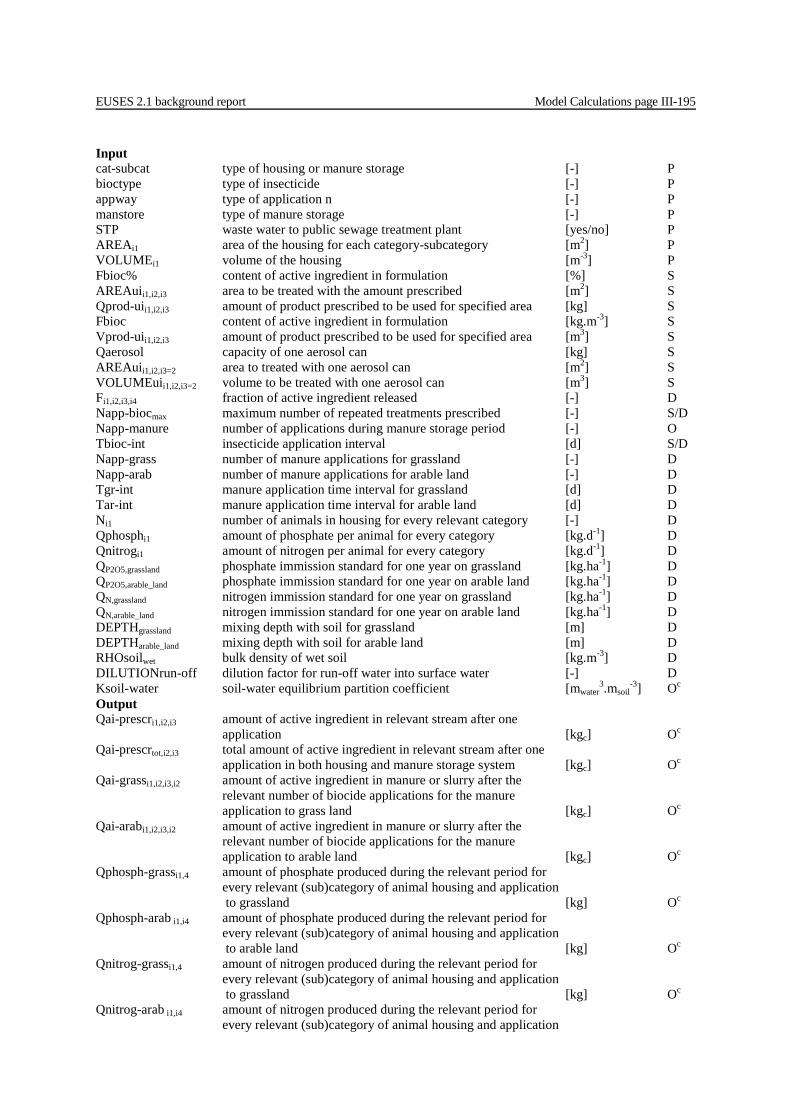
EUSES 2.1 background report Model Calculations page III-195
Input cat-subcat type of housing or manure storage [-] P bioctype type of insecticide [-] P appway type of application n [-] P manstore type of manure storage [-] P STP waste water to public sewage treatment plant [yes/no] P AREAi1 area of the housing for each category-subcategory [m2] P VOLUMEi1 volume of the housing [m-3] P Fbioc% content of active ingredient in formulation [%] S AREAuii1,i2,i3 area to be treated with the amount prescribed [m2] S Qprod-uii1,i2,i3 amount of product prescribed to be used for specified area [kg] S Fbioc content of active ingredient in formulation [kg.m-3] S Vprod-uii1,i2,i3 amount of product prescribed to be used for specified area [m3] S Qaerosol capacity of one aerosol can [kg] S AREAuii1,i2,i3=2 area to treated with one aerosol can [m2] S VOLUMEuii1,i2,i3=2 volume to be treated with one aerosol can [m3] S Fi1,i2,i3,i4 fraction of active ingredient released [-] D Napp-biocmax maximum number of repeated treatments prescribed [-] S/D Napp-manure number of applications during manure storage period [-] O Tbioc-int insecticide application interval [d] S/D Napp-grass number of manure applications for grassland [-] D Napp-arab number of manure applications for arable land [-] D Tgr-int manure application time interval for grassland [d] D Tar-int manure application time interval for arable land [d] D Ni1 number of animals in housing for every relevant category [-] D Qphosphi1 amount of phosphate per animal for every category [kg.d-1] D Qnitrogi1 amount of nitrogen per animal for every category [kg.d-1] D QP2O5,grassland phosphate immission standard for one year on grassland [kg.ha-1] D QP2O5,arable_land phosphate immission standard for one year on arable land [kg.ha-1] D QN,grassland nitrogen immission standard for one year on grassland [kg.ha-1] D QN,arable_land nitrogen immission standard for one year on arable land [kg.ha-1] D DEPTHgrassland mixing depth with soil for grassland [m] D DEPTHarable_land mixing depth with soil for arable land [m] D RHOsoilwet bulk density of wet soil [kg.m-3] D DILUTIONrun-off dilution factor for run-off water into surface water [-] D Ksoil-water soil-water equilibrium partition coefficient [mwater
3.msoil-3] Oc
Output Qai-prescri1,i2,i3 amount of active ingredient in relevant stream after one application [kgc] Oc
Qai-prescrtot,i2,i3 total amount of active ingredient in relevant stream after one application in both housing and manure storage system [kgc] Oc
Qai-grassi1,i2,i3,i2 amount of active ingredient in manure or slurry after the relevant number of biocide applications for the manure application to grass land [kgc] Oc
Qai-arabi1,i2,i3,i2 amount of active ingredient in manure or slurry after the relevant number of biocide applications for the manure application to arable land [kgc] Oc
Qphosph-grassi1,4 amount of phosphate produced during the relevant period for every relevant (sub)category of animal housing and application to grassland [kg] Oc
Qphosph-arab i1,i4 amount of phosphate produced during the relevant period for every relevant (sub)category of animal housing and application to arable land [kg] Oc
Qnitrog-grassi1,4 amount of nitrogen produced during the relevant period for every relevant (sub)category of animal housing and application to grassland [kg] Oc
Qnitrog-arab i1,i4 amount of nitrogen produced during the relevant period for every relevant (sub)category of animal housing and application

Model Calculations page III-196 EUSES 2.1 background report
to arable land [kg] Oc
PIECgrs-P2O5i1,i2,,i3,i4 concentration of active ingredient in soil based on phosphate immission standard for grassland [kgc.kg-1] O PIECarab-P2O5i1,i2,,i3,i4 concentration of active ingredient in soil based on phosphate Immission standard for arable land [kgc.kg-1] O PIECgrs-Ni1,i2,,i3,i4 concentration of active ingredient in soil based on nitrogen immission standard for grassland [kgc.kg-1] O PIECarab-Ni1,i2,,i3,i4 concentration of active ingredient in soil based on nitrogen immission standard for arable land [kgc.kg-1] O PIECgrs-pw-Pi1,i2,,i3,i4 concentration of active ingredient in pore water based on phosphate immission standard for grassland [kgc.kg-1] O PIECars-pw-Pi1,i2,,i3,i4 concentration of active ingredient in pore water based on phosphate immission standard for arable land [kgc.kg-1] O PIECgrs-pw-Ni1,i2,,i3,i4 concentration of active ingredient in pore water based on nitrogen immission standard for grassland [kgc.kg-1] O PIECars-pw-Ni1,i2,,i3,i4 concentration of active ingredient in pore water based on nitrogen immission standard for arable land [kgc.kg-1] O PIECgrs-wat-Pi1,i2,,i3,i4 concentration of active ingredient in water based on phosphate immission standard for grassland [kgc.kg-1] O PIECars-wat-Pi1,i2,,i3,i4 concentration of active ingredient in water based on phosphate immission standard for arable land [kgc.kg-1] O PIECgrs-wat-Ni1,i2,,i3,i4 concentration of active ingredient in water based on nitrogen immission standard for grassland [kgc.kg-1] O PIECars-wat-Ni1,i2,,i3,i4 concentration of active ingredient in water based on nitrogen immission standard for arable land [kgc.kg-1] O Qai-STPi1,i2,i3,i4 amount of active ingredient reaching the STP at each cleaning event [kgc.d-1] O

EUSES 2.1 background report Model Calculations page III-197
Table III-130 Default settings for calculating concentrations in surface water for compounds used as insecticides.
Category-subcategory, i1 Bioctype, i2 Appway, i3 Stream, i4
1) Dairy cows
2) Beef cattle
3) Veal calves
4) Sows in individual pens
5) Sows in groups
6) Fattening pigs
7) Laying hens in battery cages without treatment
8) Laying hens in battery cages with belt drying
9) Laying hens in battery cages with forced drying (deep pit, high-rise)
10) Laying hens in compact battery cages
11) Laying hens in free range with litter floor
12) Broilers in free range with litter floor
13) Laying hens in free range with grating floor (aviary system)
14) Parent broilers in free range with grating floor
15) Parent broilers in rearing with grating floor
16) Turkeys in free range with litter floor
17) Ducks in free range with litter floor
18) Geese in free range with litter floor
19) Wet manure storage (slurry pits)
20) Dry manure storage (manure heaps)
1) Insecticide against adult flies
2) Insecticide against bloodsucking pests
3) Larvicide
4) Insecticide against insects not affecting live stock
1) Spraying
2) Aerosol/fogging
3) Smearing
4) Sprinkling
5) Bait
6) Bait and sprinkling
1) Dry manure
2) Waste water
3) Slurry

Model Calculations page III-198 EUSES 2.1 background report Table III-131 Default settings for parameters used in calculating the amount of active ingredient applied and the amount of manure produced: Number of animals, Ni1 [-], floor
AREAi1 [m2], housing volume [m3], amount of phosphate produced, Qphosphi1, [kg.animal-1.day-1], amount of nitrogen produced, Qnitrogi1, [kg.animal-1.day-1] and the manure area for manure storage systems AREAi1=19,20 [m2]
Category-subcategory Subcategory Ni1 Qphosphi1 Qnitrogi1 AREAi1=19,20
Dry storage Wet storage (slurry)
Manure heaps Tank Lagoon
Rectangular Circular
Cattle
Dairy
Beef
Veal calves
100
125
80
0.10466
0.07123
0.01422
0.33890
0.28819
0.02382
n.r.
n.r.
n.r.
1515
495
319
1238
404
261
4086
1175
695
Pigs
Sows
Fattening pigs
individual
group
132
132
400
0.05566
0.05566
0.02033
0.07106
0.07106
0.03043
n.r.
n.r.
n.r.
369
369
369
301
301
301
823
823
985
Poultry
Laying hens
Broilers
Parent broilers
Parent broilers in rearing
Turkey
Ducks
Geese
Battery-no treatment
Battery-belt drying
Battery-deep pit high rise
Compact
Free-range litter floor
Aviary
Free-range litter floor
Free-range grating floor
Free-range grating floor
Free-range litter floor
Free-range litter floor
Free-range litter floor
21000
21000
21000
21000
10000
20000
20000
7000
9000
10000
10000
10000
0.00111
0.00111
0.00111
0.00122
0.00111
0.00111
0.00066
0.00077
0.00188
0.00230
0.00164
0.00230
0.00181
0.00181
0.00181
0.00202
0.00171
0.00171
0.00156
0.00137
0.00298
0.00482
0.00274
0.00482
n.r.
750
750
n.r.
360
n.r.
500
n.r.
n.r.
1160
470
1160
350
n.r.
n.r.
350
n.r.
330
n.r.
131
155
n.r.
n.r.
n.r.
280
n.r.
n.r.
280
n.r.
270
n.r.
107
127
n.r.
n.r.
n.r.
759
n.r.
n.r.
759
n.r.
731
n.r.
267
316
n.r.
n.r.
n.r.
n.r. not relevant
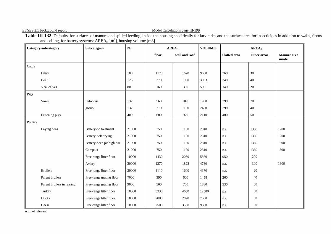
EUSES 2.1 background report Model Calculations page III-199 Table III-132 Defaults for surfaces of manure and spilled feeding, inside the housing specifically for larvicides and the surface area for insecticides in addition to walls, floors and ceiling, for battery systems: AREAi1 [m2], housing volume [m3].
Category-subcategory Subcategory Ni1 AREAi1
floor wall and roof
VOLUMEi1 AREAi1
Slatted area Other areas Manure area inside
Cattle
Dairy
Beef
Veal calves
100
125
80
1170
370
160
1670
1000
330
9630
3063
590
360
340
140
30
40
20
Pigs
Sows
Fattening pigs
individual
group
132
132
400
560
710
600
910
1160
970
1960
2480
2110
390
290
400
70
40
50
Poultry
Laying hens
Broilers
Parent broilers
Parent broilers in rearing
Turkey
Ducks
Geese
Battery-no treatment
Battery-belt drying
Battery-deep pit high rise
Compact
Free-range litter floor
Aviary
Free-range litter floor
Free-range grating floor
Free-range grating floor
Free-range litter floor
Free-range litter floor
Free-range litter floor
21000
21000
21000
21000
10000
20000
20000
7000
9000
10000
10000
10000
750
750
750
750
1430
1270
1110
390
500
3330
2000
2500
1100
1100
1100
1100
2030
1822
1600
600
750
4650
2820
3500
2810
2810
2810
2810
5360
4780
4170
1458
1880
12500
7500
9380
n.r.
n.r.
n.r.
n.r.
950
n.r.
n.r.
260
330
n.r
n.r.
n.r.
1360
1360
1360
1360
200
300
20
40
60
60
60
60
1200
1200
600
300
1600
n.r. not relevant
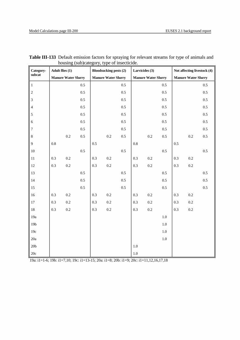
Model Calculations page III-200 EUSES 2.1 background report
Table III-133 Default emission factors for spraying for relevant streams for type of animals and housing (sub)category, type of insecticide.
Category-subcat
Adult flies (1)
Manure Water Slurry
Bloodsucking pests (2)
Manure Water Slurry
Larvicides (3)
Manure Water Slurry
Not affecting livestock (4)
Manure Water Slurry
1
2
3
4
5
6
7
8
9
10
11
12
13
14
15
16
17
18
19a
19b
19c
20a
20b
20c
0.5
0.5
0.5
0.5
0.5
0.5
0.5
0.2 0.5
0.8
0.5
0.3 0.2
0.3 0.2
0.5
0.5
0.5
0.3 0.2
0.3 0.2
0.3 0.2
0.5
0.5
0.5
0.5
0.5
0.5
0.5
0.2 0.5
0.5
0.5
0.3 0.2
0.3 0.2
0.5
0.5
0.5
0.3 0.2
0.3 0.2
0.3 0.2
0.5
0.5
0.5
0.5
0.5
0.5
0.5
0.2 0.5
0.8
0.5
0.3 0.2
0.3 0.2
0.5
0.5
0.5
0.3 0.2
0.3 0.2
0.3 0.2
1.0
1.0
1.0
1.0
1.0
1.0
0.5
0.5
0.5
0.5
0.5
0.5
0.5
0.2 0.5
0.5
0.5
0.3 0.2
0.3 0.2
0.5
0.5
0.5
0.3 0.2
0.3 0.2
0.3 0.2
19a: i1=1-6; 19b: i1=7,10; 19c: i1=13-15; 20a: i1=8; 20b: i1=9; 20c: i1=11,12,16,17,18

EUSES 2.1 background report Model Calculations page III-201
Table III-134 Default emission factors for aerosol for relevant streams for type of animals and housing (sub)category, type of insecticide.
Category-subcat
Adult flies (1)
Manure Water Slurry
Bloodsucking pests (2)
Manure Water Slurry
Larvicides (3)
Manure Water Slurry
Not affecting livestock (4)
Manure Water Slurry
1
2
3
4
5
6
7
8
9
10
11
12
13
14
15
16
17
18
19a
19b
19c
20a
20b
20c
0.35
0.35
0.35
0.35
0.35
0.35
0.35
0.10 0.35
0.35
0.35
0.25 0.10
0.25 0.10
0.35
0.35
0.35
0.25 0.10
0.25 0.10
0.25 0.10
0.35
0.35
0.35
0.35
0.35
0.35
0.35
0.10 0.35
0.35
0.35
0.25 0.10
0.25 0.10
0.35
0.35
0.35
0.25 0.10
0.25 0.10
0.25 0.10
0.35
0.35
0.35
0.35
0.35
0.35
0.35
0.10 0.35
0.35
0.35
0.25 0.10
0.25 0.10
0.35
0.35
0.35
0.25 0.10
0.25 0.10
0.25 0.10
1.0
1.0
1.0
1.0
1.0
1.0
0.35
0.35
0.35
0.35
0.35
0.35
0.35
0.10 0.35
0.35
0.35
0.25 0.10
0.25 0.10
0.35
0.35
0.35
0.25 0.10
0.25 0.10
0.25 0.10
19a: i1=1-6; 19b: i1=7,10; 19c: i1=13-15; 20a: i1=8; 20b: i1=9; 20c: i1=11,12,16,17,18
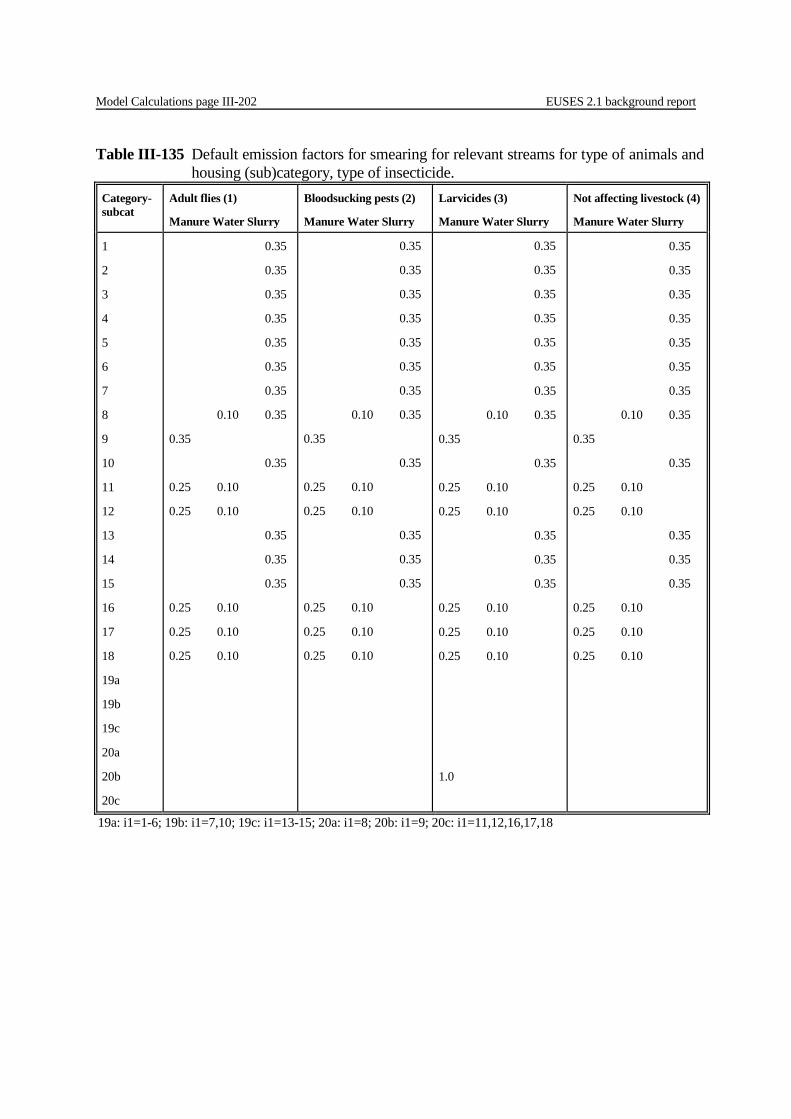
Model Calculations page III-202 EUSES 2.1 background report
Table III-135 Default emission factors for smearing for relevant streams for type of animals and housing (sub)category, type of insecticide.
Category-subcat
Adult flies (1)
Manure Water Slurry
Bloodsucking pests (2)
Manure Water Slurry
Larvicides (3)
Manure Water Slurry
Not affecting livestock (4)
Manure Water Slurry
1
2
3
4
5
6
7
8
9
10
11
12
13
14
15
16
17
18
19a
19b
19c
20a
20b
20c
0.35
0.35
0.35
0.35
0.35
0.35
0.35
0.10 0.35
0.35
0.35
0.25 0.10
0.25 0.10
0.35
0.35
0.35
0.25 0.10
0.25 0.10
0.25 0.10
0.35
0.35
0.35
0.35
0.35
0.35
0.35
0.10 0.35
0.35
0.35
0.25 0.10
0.25 0.10
0.35
0.35
0.35
0.25 0.10
0.25 0.10
0.25 0.10
0.35
0.35
0.35
0.35
0.35
0.35
0.35
0.10 0.35
0.35
0.35
0.25 0.10
0.25 0.10
0.35
0.35
0.35
0.25 0.10
0.25 0.10
0.25 0.10
1.0
0.35
0.35
0.35
0.35
0.35
0.35
0.35
0.10 0.35
0.35
0.35
0.25 0.10
0.25 0.10
0.35
0.35
0.35
0.25 0.10
0.25 0.10
0.25 0.10
19a: i1=1-6; 19b: i1=7,10; 19c: i1=13-15; 20a: i1=8; 20b: i1=9; 20c: i1=11,12,16,17,18

EUSES 2.1 background report Model Calculations page III-203
Table III-136 Default emission factors for sprinkling for relevant streams for type of animals and housing (sub)category, type of insecticide.
Category-subcat
Adult flies (1)
Manure Water Slurry
Bloodsucking pests (2)
Manure Water Slurry
Larvicides (3)
Manure Water Slurry
Not affecting livestock(4)
Manure Water Slurry
1
2
3
4
5
6
7
8
9
10
11
12
13
14
15
16
17
18
19a
19b
19c
20a
20b
20c
0.90
0.90
0.90
0.90
0.90
0.90
0.90
0.90
0.90
0.80 0.10
0.80 0.10
0.90
0.90
0.90
0.80 0.10
0.80 0.10
0.80 0.10
0.90
0.90
0.90
0.90
0.90
0.90
0.90
0.80
0.90
0.80 0.10
0.80 0.10
0.90
0.90
0.90
0.80 0.10
0.80 0.10
0.80 0.10
0.90
0.10 0.90
0.90
0.90
0.80 0.10
0.80 0.10
0.90
0.90
0.90
0.80 0.10
0.80 0.10
0.80 0.10
1.0
1.0
1.0
1.0
1.0
1.0
0.90
0.90
0.90
0.90
0.90
0.90
0.90
0.80
0.90
0.80 0.10
0.80 0.10
0.90
0.90
0.90
0.80 0.10
0.80 0.10
0.80 0.10
19a: i1=1-6; 19b: i1=7,10; 19c: i1=13-15; 20a: i1=8; 20b: i1=9; 20c: i1=11,12,16,17,18

Model Calculations page III-204 EUSES 2.1 background report
Table III-137 Default emission factors for bait for relevant streams for type of animals and housing (sub)category, type of insecticide.
Category-subcat
Adult flies (1)
Manure Water Slurry
Bloodsucking pests (2)
Manure Water Slurry
Larvicides (3)
Manure Water Slurry
Not affecting livestock (4)
Manure Water Slurry
1
2
3
4
5
6
7
8
9
10
11
12
13
14
15
16
17
18
19a
19b
19c
20a
20b
20c
0.50
0.50
0.50
0.50
0.50
0.50
0.50
0.45 0.50
0.50
0.50
0.05 0.45
0.05 0.45
0.50
0.50
0.50
0.05 0.45
0.05 0.45
0.05 0.45
0.50
0.50
0.50
0.50
0.50
0.50
0.50
0.45 0.50
0.40
0.50
0.05 0.45
0.05 0.45
0.50
0.50
0.50
0.05 0.45
0.05 0.45
0.05 0.45
0.50
0.50
0.50
0.50
0.50
0.50
0.50
0.45 0.50
0.40
0.50
0.05 0.45
0.05 0.45
0.50
0.50
0.50
0.05 0.45
0.05 0.45
0.05 0.45
19a: i1=1-6; 19b: i1=7,10; 19c: i1=13-15; 20a: i1=8; 20b: i1=9; 20c: i1=11,12,16,17,18
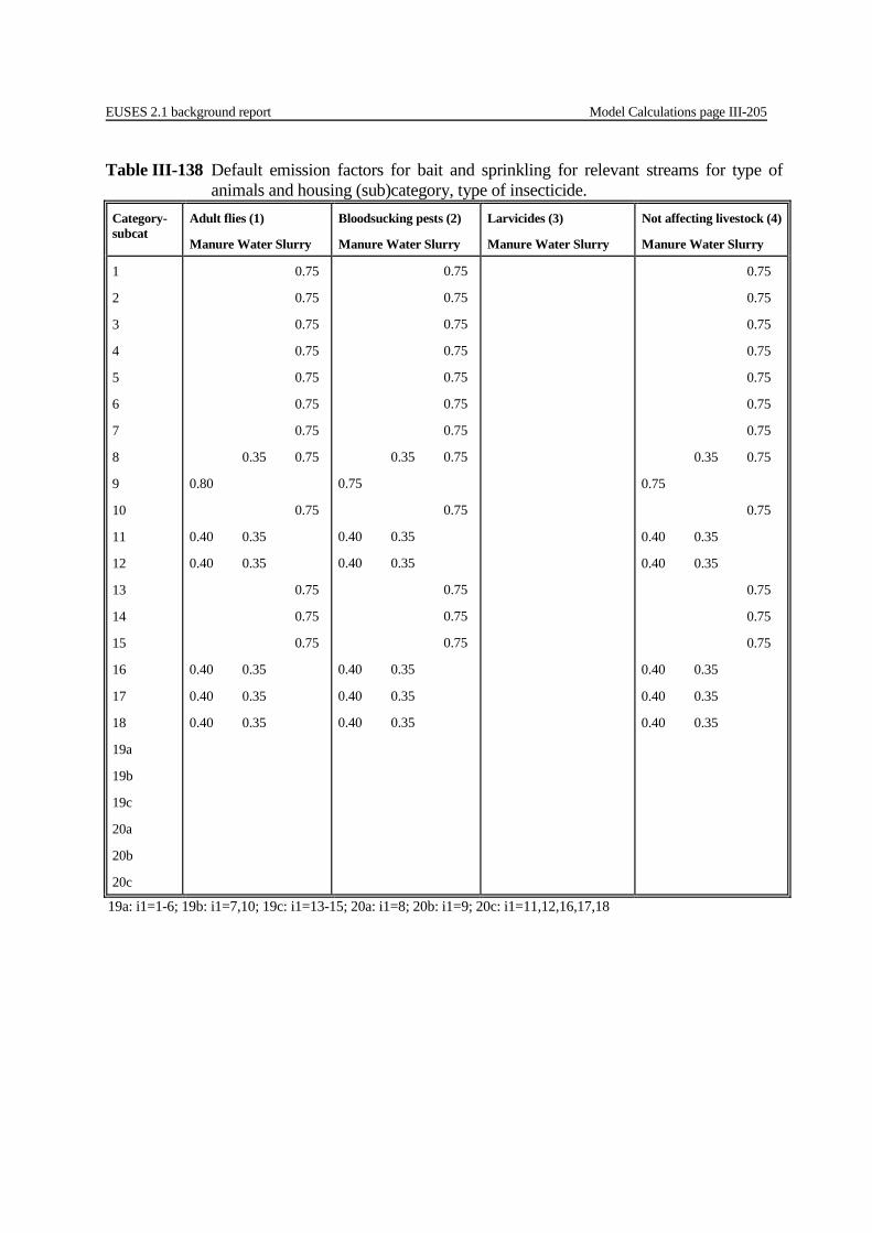
EUSES 2.1 background report Model Calculations page III-205
Table III-138 Default emission factors for bait and sprinkling for relevant streams for type of animals and housing (sub)category, type of insecticide.
Category-subcat
Adult flies (1)
Manure Water Slurry
Bloodsucking pests (2)
Manure Water Slurry
Larvicides (3)
Manure Water Slurry
Not affecting livestock (4)
Manure Water Slurry
1
2
3
4
5
6
7
8
9
10
11
12
13
14
15
16
17
18
19a
19b
19c
20a
20b
20c
0.75
0.75
0.75
0.75
0.75
0.75
0.75
0.35 0.75
0.80
0.75
0.40 0.35
0.40 0.35
0.75
0.75
0.75
0.40 0.35
0.40 0.35
0.40 0.35
0.75
0.75
0.75
0.75
0.75
0.75
0.75
0.35 0.75
0.75
0.75
0.40 0.35
0.40 0.35
0.75
0.75
0.75
0.40 0.35
0.40 0.35
0.40 0.35
0.75
0.75
0.75
0.75
0.75
0.75
0.75
0.35 0.75
0.75
0.75
0.40 0.35
0.40 0.35
0.75
0.75
0.75
0.40 0.35
0.40 0.35
0.40 0.35
19a: i1=1-6; 19b: i1=7,10; 19c: i1=13-15; 20a: i1=8; 20b: i1=9; 20c: i1=11,12,16,17,18
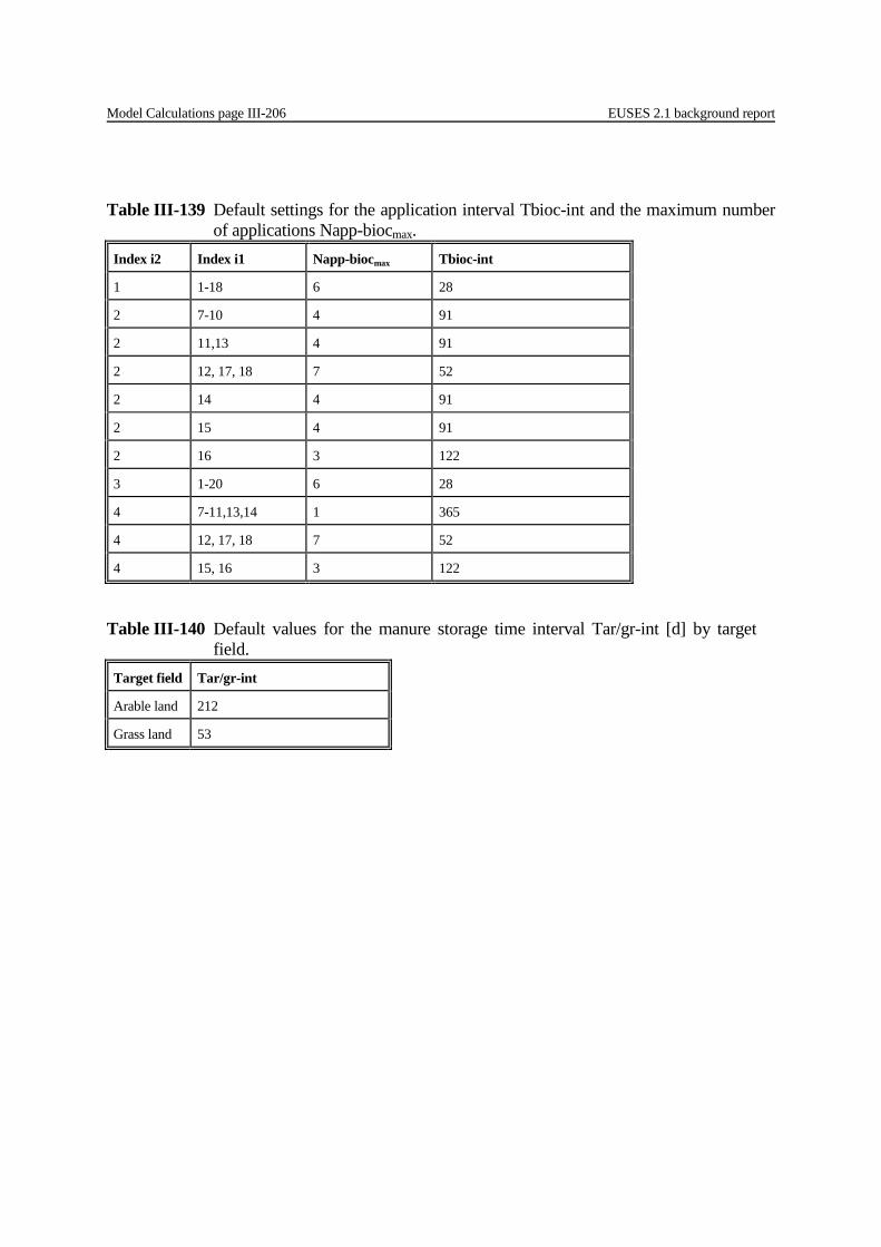
Model Calculations page III-206 EUSES 2.1 background report
Table III-139 Default settings for the application interval Tbioc-int and the maximum number of applications Napp-biocmax.
Index i2 Index i1 Napp-biocmax Tbioc-int
1 1-18 6 28
2 7-10 4 91
2 11,13 4 91
2 12, 17, 18 7 52
2 14 4 91
2 15 4 91
2 16 3 122
3 1-20 6 28
4 7-11,13,14 1 365
4 12, 17, 18 7 52
4 15, 16 3 122
Table III-140 Default values for the manure storage time interval Tar/gr-int [d] by target field.
Target field Tar/gr-int
Arable land 212
Grass land 53
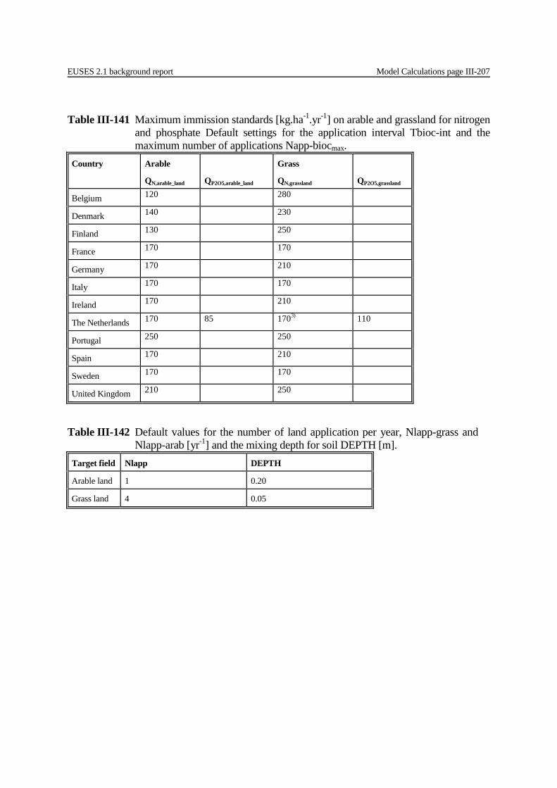
EUSES 2.1 background report Model Calculations page III-207
Table III-141 Maximum immission standards [kg.ha-1.yr-1] on arable and grassland for nitrogen and phosphate Default settings for the application interval Tbioc-int and the maximum number of applications Napp-biocmax.
Country Arable
QN,arable_land
QP2O5,arable_land
Grass
QN,grassland
QP2O5,grassland
Belgium 120 280
Denmark 140 230
Finland 130 250
France 170 170
Germany 170 210
Italy 170 170
Ireland 170 210
The Netherlands 170 85 1703) 110
Portugal 250 250
Spain 170 210
Sweden 170 170
United Kingdom 210 250
Table III-142 Default values for the number of land application per year, Nlapp-grass and Nlapp-arab [yr-1] and the mixing depth for soil DEPTH [m].
Target field Nlapp DEPTH
Arable land 1 0.20
Grass land 4 0.05
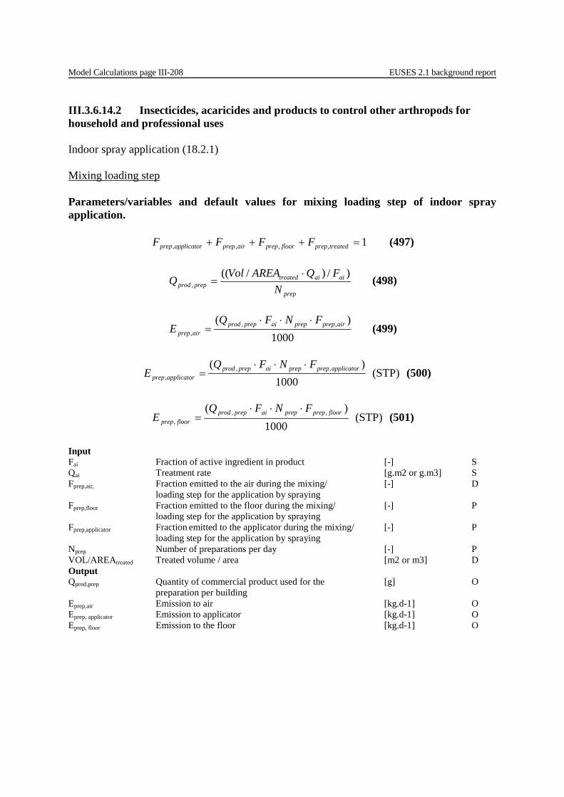
Model Calculations page III-208 EUSES 2.1 background report
III.3.6.14.2 Insecticides, acaricides and products to control other arthropods for household and professional uses Indoor spray application (18.2.1) Mixing loading step Parameters/variables and default values for mixing loading step of indoor spray application.
1,,,, =+++ treatedprepfloorprepairprepapplicatorprep FFFF (497)
prep
aiaitreatedprepprod N
FQAREAVolQ
)/)/((,
⋅= (498)
1000)( ,,
,airprepprepaiprepprod
airprep
FNFQE
⋅⋅⋅= (499)
1000)( ,,
,applicatorprepprepaiprepprod
applicatorprep
FNFQE
⋅⋅⋅= (STP) (500)
1000)( ,,
,floorprepprepaiprepprod
floorprep
FNFQE
⋅⋅⋅= (STP) (501)
Input Fai Fraction of active ingredient in product [-] S Qai Treatment rate [g.m2 or g.m3] S Fprep,air, Fraction emitted to the air during the mixing/ [-] D
loading step for the application by spraying Fprep,floor Fraction emitted to the floor during the mixing/ [-] P loading step for the application by spraying Fprep,applicator Fraction emitted to the applicator during the mixing/ [-] P loading step for the application by spraying Nprep Number of preparations per day [-] P VOL/AREAtreated Treated volume / area [m2 or m3] D Output Qprod,prep Quantity of commercial product used for the [g] O preparation per building Eprep,air Emission to air [kg.d-1] O Eprep, applicator Emission to applicator [kg.d-1] O Eprep, floor Emission to the floor [kg.d-1] O

EUSES 2.1 background report Model Calculations page III-209
Table III-143 Default values for the mixing step of the indoor spray application. Parameter Value
Nprep House (1, professional and non-professional), larger building (3, professional)
Fprep,air 0
Fprep,applicator Liquid (0.0012), powder (0), granules (0)
VOLUMEtreated 58
AREAtreated General surface treatment (22), targeted spot (2), larger building treatment (3280)
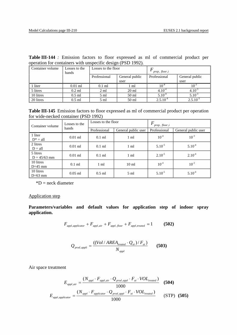
Model Calculations page III-210 EUSES 2.1 background report
Table III-144 : Emission factors to floor expressed as ml of commercial product per operation for containers with unspecific design (PSD 1992).
Container volume Losses to the hands
Losses to the floor ifloorprepF ,,
Professional General public user
Professional General public user
1 liter 0.01 ml 0.1 ml 1 ml 10-4 10-3 5 litres 0.2 ml 2 ml 20 ml 4.10-4 4.10-3 10 litres 0.5 ml 5 ml 50 ml 5.10-4 5.10-3 20 litres 0.5 ml 5 ml 50 ml 2.5.10-4 2.5.10-3
Table III-145 Emission factors to floor expressed as ml of commercial product per operation for wide-necked container (PSD 1992)
Container volume Losses to the hands
Losses to the floor ifloorprepF ,,
Professional General public user Professional General public user 1 liter D* = all 0.01 ml 0.1 ml 1 ml 10-4 10-3
2 litres D = all 0.01 ml 0.1 ml 1 ml 5.10-5 5.10-4
5 litres D = 45/63 mm 0.01 ml 0.1 ml 1 ml 2.10-5 2.10-4
10 litres D=45 mm 0.1 ml 1 ml 10 ml 10-4 10-3
10 litres D=63 mm 0.05 ml 0.5 ml 5 ml 5.10-5 5.10-4
*D = neck diameter Application step Parameters/variables and default values for application step of indoor spray application.
1,,,, =+++ treatedapplfloorapplairapplapplicatorappl FFFF (502)
appl
aiaitreatedappliprod N
FQAREAVolQ
)/)/((,
⋅= (503)
Air space treatment
1000)( ,,
,treatedaiapplprodairapplappl
airappl
VOLFQFNE
⋅⋅⋅⋅= (504)
1000)( ,
,treatedaiapplprodapplicatorappl
applicatorappl
VOLFQFNE
⋅⋅⋅⋅= (STP) (505)
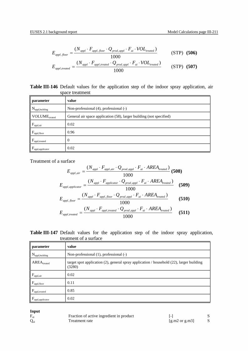
EUSES 2.1 background report Model Calculations page III-211
1000)( ,,
,treatedaiapplprodfloorapplappl
floorappl
VOLFQFNE
⋅⋅⋅⋅= (STP) (506)
1000)( ,,
,treatedaiapplprodtreatedapplappl
treatedappl
VOLFQFNE
⋅⋅⋅⋅= (STP) (507)
Treatment of a surface
1000)( ,,
,treatedaiapplprodairapplappl
airappl
AREAFQFNE
⋅⋅⋅⋅= (508)
1000)( ,
,treatedaiapplprodapplicatorappl
applicatorappl
AREAFQFNE
⋅⋅⋅⋅= (509)
1000)( ,,
,treatedaiapplprodfloorapplappl
floorappl
AREAFQFNE
⋅⋅⋅⋅= (510)
1000)( ,,
,treatedaiapplprodtreatedapplappl
treatedappl
AREAFQFNE
⋅⋅⋅⋅= (511)
Input Fai Fraction of active ingredient in product [-] S Qai Treatment rate [g.m2 or g.m3] S
Table III-146 Default values for the application step of the indoor spray application, air space treatment
parameter value
Nappl,building Non-professional (4), professional (-)
VOLUMEtreated General air space application (58), larger building (not specified)
Fappl,air 0.02
Fappl,floor 0.96
Fappl,treated 0
Fappl,applicator 0.02
Table III-147 Default values for the application step of the indoor spray application, treatment of a surface
parameter value
Nappl,building Non-professional (1), professional (-)
AREAtreated target spot application (2), general spray application / household (22), larger building (3280)
Fappl,air 0.02
Fappl,floor 0.11
Fappl,treated 0.85
Fappl,applicator 0.02

Model Calculations page III-212 EUSES 2.1 background report
Fappl,air, Fraction emitted to the air during application [-] P Fappl,floor Fraction emitted to the floor during application [-] P Fappl,applicator Fraction emitted to the applicator during [-] P application Fappl,treated Fraction emitted to the treated surfaces during [-] P application Nappl Number of applications per day per building [d-1] P VOL/AREAtreated Treated volume / area [m2 or m3] D Output Qprod,appl uantity of commercial product used for the [g] O preparation per building Eappl,air Emission to air [kg.d-1] O Eappl, applicator Emission to applicator [kg.d-1] O Eappl, floor Emission to the floor [kg.d-1] O Eappl,treated Emission to treated surface/volume [kg.d-1] O Cleaning step Parameters/variables and default values for cleaning step of indoor spray application. Release to air Ecleaning,air = 0 (outdoor air) No release to waste water
wapplicatorapplicatornapplicatioapplicatorprepwapplicator FEEE ,,,, )( ⋅+= (512)
CEwtreatednapplicatiofloornapplicatiofloorprepwtreated FFEEEE ⋅⋅++= )( ,,,, (513) If 100% of the coveralls are disposable, then Fapplicator,w = 1 and Fapplicator,ww = 0. If 100% of the surfaces are cleaned by vacuum/broom, then Fw = 1 and Fww = 0. Input Eprep,applicator Emission to applicator during preparation step [kd.d-1] O Eapplication,applicator Emission to applicator during the application step [kg.d-1] O Fapplicator,w Fraction emitted to solid waste from applicator [-] P Eprep,floor Emission to the floor during preparation [kg.d-1] O Eapplication,floor Emission to the floor during application [kg.d-1] O Eapplication,treated Emission to treated surfaces during the application step [kg.d-1] O Fw Fraction emitted to solid waste [-] D FCE Cleaning efficiency [-] D Output Eapplicator,w Emission from applicator to solid waste during cleaning [kg.d-1] Etreated,w Emission from floor/treated surfaces to solid waste [kg.d-1] No release to municipal wastes
wwapplicatorapplicatornapplicatioapplicatorprepwwapplicator FEEE ,,,, )( ⋅+= (514)
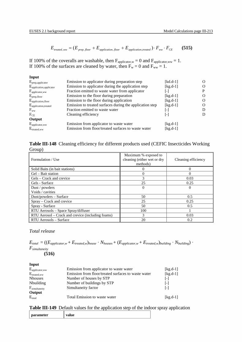
EUSES 2.1 background report Model Calculations page III-213
CEwwtreatednapplicatiofloornapplicatiofloorprepwwtreated FFEEEE ⋅⋅++= )( ,,,, (515) If 100% of the coveralls are washable, then Fapplicator,w = 0 and Fapplicator,ww = 1. If 100% of the surfaces are cleaned by water, then Fw = 0 and Fww = 1. Input Eprep,applicator Emission to applicator during preparation step [kd.d-1] O Eapplication,applicator Emission to applicator during the application step [kg.d-1] O Fapplicator,ww Fraction emitted to waste water from applicator [-] P Eprep,floor Emission to the floor during preparation [kg.d-1] O Eapplication,floor Emission to the floor during application [kg.d-1] O Eapplication,treated Emission to treated surfaces during the application step [kg.d-1] O Fww Fraction emitted to waste water [-] D FCE Cleaning efficiency [-] D Output Eapplicator,ww Emission from applicator to waste water [kg.d-1] Etreated,ww Emission from floor/treated surfaces to waste water [kg.d-1] Table III-148 Cleaning efficiency for different products used (CEFIC Insecticides Working Group)
Formulation / Use Maximum % exposed to
cleaning (either wet or dry methods)
Cleaning efficiency
Solid Baits (in bait stations) 0 0 Gel – Bait station 0 0 Gels – Crack and crevice 3 0.03 Gels - Surface 25 0.25 Dust / powders Voids / cavities
0 0
Dust/powders – Surface 50 0.5 Spray – Crack and crevice 25 0.25 Spray - Surface 50 0.5 RTU Aerosols – Space Spray/diffuser 100 1 RTU Aerosol – Crack and crevice (including foams) 3 0.03 RTU Aerosols – Surface 20 0.2
Total release Etotal = ((Eapplicator,w + Etreated,w)house · Nhouses + (Eapplicator,w + Etreated,w)building · Nbuilding) · Fsimultaneity
(516) Input Eapplicator,ww Emission from applicator to waste water [kg.d-1] Etreated,ww Emission from floor/treated surfaces to waste water [kg.d-1] Nhouses Number of houses by STP [-] Nbuilding Number of buildings by STP [-] Fsimultaneity Simultaneity factor [-] Output Etotal Total Emission to waste water [kg.d-1] Table III-149 Default values for the application step of the indoor spray application parameter value

Model Calculations page III-214 EUSES 2.1 background report
Nhouses 4000
Nbuilding 1000
Fsimultaneity 0.055
Indoor gel application (18.2.2) Mixing / loading step No emission during mixing / loading. Application step Parameters/variables and default values for application step of indoor gel application.
1000)( ,,intint,
,buildingapplairappltreatedaipopoprod
airappl
NFAREAFNQE
⋅⋅⋅⋅⋅= (517)
1000)( ,,intint,
,buildingapplapplicatorappltreatedaipopoprod
applicatorappl
NFAREAFNQE
⋅⋅⋅⋅⋅= (STP) (518)
1000)( ,,intint,
,buildingappltreatedappltreatedaipopoprod
treatedappl
NFAREAFNQE
⋅⋅⋅⋅⋅= (STP) (519)
Input Fai Fraction of active ingredient in product [-] S Npoint Number of gel points per square meter [point.m-2] P Nappl Number of applications per day per building [d-1] P Fappl,air, Fraction emitted to the air during application [-] P Fappl,applicator Fraction emitted to the applicator during application [-] P Fappl,treated Fraction emitted to the treated surfaces during application [-] P AREAtreated Area treated with the product [m2] D Qprod,point Quantity of commercial product applied per point of gel [g.point-1] S Output Eappl,air Emission to air [kg.d-1] O Eappl, applicator Emission to applicator [kg.d-1] O Eappl,treated Emission to treated surface/volume [kg.d-1] O Table III-150 Default values for the application step of the indoor gel application parameter value
Nappl,building Household (6), larger building (-)
Npoint Preventive treatment or low infestation level (1),
curative treatment or high infestation level (3)
AREAtreated Household (22), larger building (3280)
Fappl,air 0
Fappl,applicator 0

EUSES 2.1 background report Model Calculations page III-215
Fappl,treated 1
Cleaning step The calculation method is mutatis mutandis the same as used for spray application. Total release The calculation method is mutatis mutandis the same as used for spray application. Indoor application of powders by dusting (18.2.3) Mixing / loading step Parameters/variables and default values for mixing/loading step of indoor application of powders by dusting.
1000)( ,,,
,airprepbuildingprepaiprepprod
airprep
FNFQE
⋅⋅⋅= (520)
1000)( ,,,
,floorprepbuildingprepaiprepprod
floorprep
FNFQE
⋅⋅⋅= (STP) (521)
1000)( ,,,
,applicatorprepbuildingprepaiprepprod
applicatorprep
FNFQE
⋅⋅⋅= (STP) (522)
Input Fai Fraction of active ingredient in product [-] S Nprep Number of preparations per dayper building [d-1] P Output Qprod,prep Quantity of commercial product used for [g] S the preparation per building Eprep,air Emission to air [kg.d-1] O Eprep, applicator Emission to applicator [kg.d-1] O Eprep, floor Emission to the floor [kg.d-1] O Table III-151 Default values for the mixing/loading step of the indoor application of powders
by dusting parameter value
Nprep,building House (1), larger building (3)
Fprep,air 0
Fprep,applicator 0
Fprep,floor 0.01
Application step Parameters/variables and default values for application step of indoor application of powders by dusting.
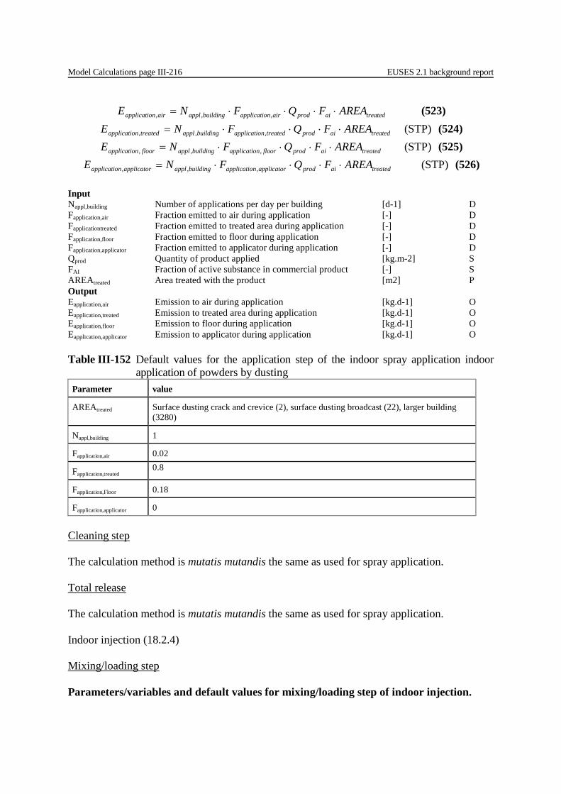
Model Calculations page III-216 EUSES 2.1 background report
treatedaiprodairnapplicatiobuildingapplairnapplicatio AREAFQFNE ⋅⋅⋅⋅= ,,, (523)
treatedaiprodtreatednapplicatiobuildingappltreatednapplicatio AREAFQFNE ⋅⋅⋅⋅= ,,, (STP) (524)
treatedaiprodfloornapplicatiobuildingapplfloornapplicatio AREAFQFNE ⋅⋅⋅⋅= ,,, (STP) (525)
treatedaiprodapplicatornapplicatiobuildingapplapplicatornapplicatio AREAFQFNE ⋅⋅⋅⋅= ,,, (STP) (526) Input Nappl,building Number of applications per day per building [d-1] D Fapplication,air Fraction emitted to air during application [-] D Fapplicationtreated Fraction emitted to treated area during application [-] D Fapplication,floor Fraction emitted to floor during application [-] D Fapplication,applicator Fraction emitted to applicator during application [-] D Qprod Quantity of product applied [kg.m-2] S FAI Fraction of active substance in commercial product [-] S AREAtreated Area treated with the product [m2] P Output Eapplication,air Emission to air during application [kg.d-1] O Eapplication,treated Emission to treated area during application [kg.d-1] O Eapplication,floor Emission to floor during application [kg.d-1] O Eapplication,applicator Emission to applicator during application [kg.d-1] O Table III-152 Default values for the application step of the indoor spray application indoor
application of powders by dusting Parameter value
AREAtreated Surface dusting crack and crevice (2), surface dusting broadcast (22), larger building (3280)
Nappl,building 1
Fapplication,air 0.02
Fapplication,treated 0.8
Fapplication,Floor 0.18
Fapplication,applicator 0
Cleaning step The calculation method is mutatis mutandis the same as used for spray application. Total release The calculation method is mutatis mutandis the same as used for spray application. Indoor injection (18.2.4) Mixing/loading step Parameters/variables and default values for mixing/loading step of indoor injection.
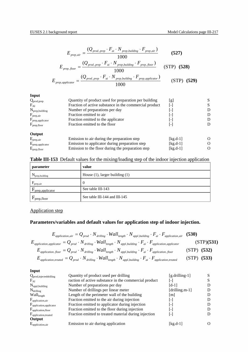
EUSES 2.1 background report Model Calculations page III-217
1000)( ,,,
,airprepbuildingprepaiprepprod
airprep
FNFQE
⋅⋅⋅= (527)
1000)( ,,,
,floorprepbuildingprepaiprepprod
floorprep
FNFQE
⋅⋅⋅= (STP) (528)
1000)( ,,,
,applicatorprepbuildingprepaiprepprod
applicatorprep
FNFQE
⋅⋅⋅= (STP) (529)
Input Qprod,prep Quantity of product used for preparation per building [g] S FAI Fraction of active substance in the commercial product [-] S Nprep,building Number of preparations per day [-] D Fprep,air Fraction emitted to air [-] D Fprep,applicator Fraction emitted to the applicator [-] D Fprep,floor Fraction emitted to the floor [-] D Output Eprep,air Emission to air during the preparation step [kg.d-1] O Eprep,applicator Emission to applicator during preparation step [kg.d-1] O Eprep,floor Emission to the floor during the preparation step [kg.d-1] O Table III-153 Default values for the mixing/loading step of the indoor injection application parameter value
Nprep,building House (1), larger building (1)
Fprep,air 0
Fprep,applicator See table III-143
Fprep,floor See table III-144 and III-145
Application step Parameters/variables and default values for application step of indoor injection.
airnapplicatioaibuildingappllengthdrillingprodairnapplicatio FFNWallNQE ,,, ⋅⋅⋅⋅⋅= (530)
applicatornapplicatioaibuildingappllengthdrillingprodapplicatornapplicatio FFNWallNQE ,,, ⋅⋅⋅⋅⋅= (STP)(531)
floornapplicatioaibuildingappllengthdrillingprodfloornapplicatio FFNWallNQE ,,, ⋅⋅⋅⋅⋅= (STP) (532)
treatednapplicatioaibuildingappllengthdrillingprodtreatednapplicatio FFNWallNQE ,,, ⋅⋅⋅⋅⋅= (STP) (533) Input Qprod,injecteddrilling Quantity of product used per drilling [g.drilling-1] S FAI raction of active substance in the commercial product [-] S Nappl,building Number of preparations per day [d-1] D Ndrilling Number of drillings per linear meter [drilling.m-1] D Walllength Length of the perimeter wall of the building [m] D Fapplication,air Fraction emitted to the air during injection [-] D Fapplication,applicator Fraction emitted to applicator during injection [-] D Fapplication,floor Fraction emitted to the floor during injection [-] D Fapplication,treated Fraction emitted to treated material during injection [-] D Output Eapplication,air Emission to air during application [kg.d-1] O
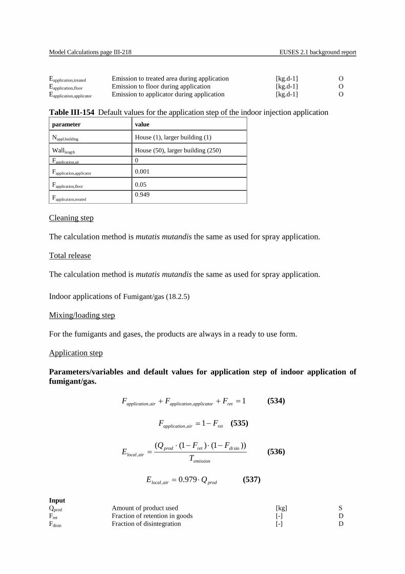
Model Calculations page III-218 EUSES 2.1 background report
Eapplication,treated Emission to treated area during application [kg.d-1] O Eapplication,floor Emission to floor during application [kg.d-1] O Eapplication,applicator Emission to applicator during application [kg.d-1] O Table III-154 Default values for the application step of the indoor injection application parameter value
Nappl,building House (1), larger building (1)
Walllength House (50), larger building (250) Fapplication,air 0
Fapplication,applicator 0.001
Fapplication,floor 0.05
Fapplication,treated 0.949
Cleaning step The calculation method is mutatis mutandis the same as used for spray application. Total release The calculation method is mutatis mutandis the same as used for spray application. Indoor applications of Fumigant/gas (18.2.5) Mixing/loading step For the fumigants and gases, the products are always in a ready to use form. Application step Parameters/variables and default values for application step of indoor application of fumigant/gas.
1,, =++ retapplicatornapplicatioairnapplicatio FFF (534)
retairnapplicatio FF −= 1, (535)
emission
diretprodairlocal T
FFQE
))1()1(( sin,
−⋅−⋅= (536)
prodairlocal QE ⋅= 979.0, (537)
Input Qprod Amount of product used [kg] S Fret Fraction of retention in goods [-] D Fdisin Fraction of disintegration [-] D
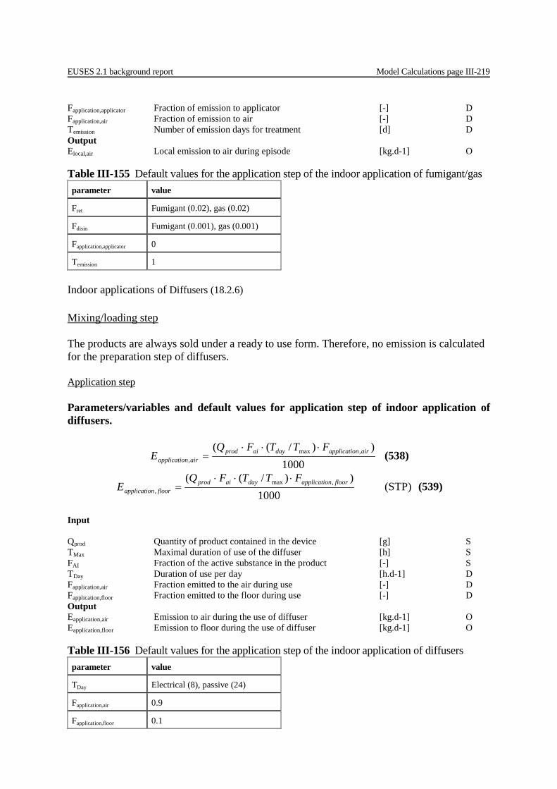
EUSES 2.1 background report Model Calculations page III-219
Fapplication,applicator Fraction of emission to applicator [-] D Fapplication,air Fraction of emission to air [-] D Temission Number of emission days for treatment [d] D Output Elocal,air Local emission to air during episode [kg.d-1] O Table III-155 Default values for the application step of the indoor application of fumigant/gas parameter value
Fret Fumigant (0.02), gas (0.02)
Fdisin Fumigant (0.001), gas (0.001)
Fapplication,applicator 0
Temission 1
Indoor applications of Diffusers (18.2.6) Mixing/loading step The products are always sold under a ready to use form. Therefore, no emission is calculated for the preparation step of diffusers. Application step Parameters/variables and default values for application step of indoor application of diffusers.
1000))/(( ,max
,airnapplicatiodayaiprod
airnapplicatio
FTTFQE
⋅⋅⋅= (538)
1000))/(( ,max
,floornapplicatiodayaiprod
floornapplicatio
FTTFQE
⋅⋅⋅= (STP) (539)
Input Qprod Quantity of product contained in the device [g] S TMax Maximal duration of use of the diffuser [h] S FAI Fraction of the active substance in the product [-] S TDay Duration of use per day [h.d-1] D Fapplication,air Fraction emitted to the air during use [-] D Fapplication,floor Fraction emitted to the floor during use [-] D Output Eapplication,air Emission to air during the use of diffuser [kg.d-1] O Eapplication,floor Emission to floor during the use of diffuser [kg.d-1] O Table III-156 Default values for the application step of the indoor application of diffusers parameter value
TDay Electrical (8), passive (24)
Fapplication,air 0.9
Fapplication,floor 0.1
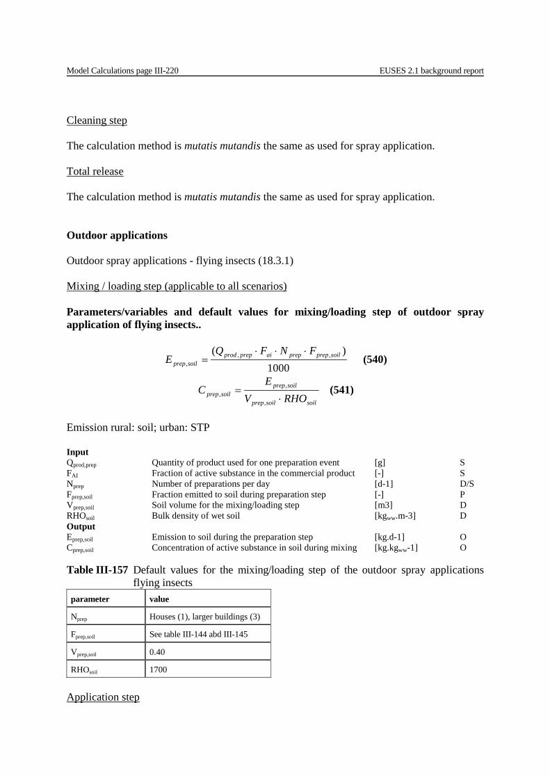
Model Calculations page III-220 EUSES 2.1 background report
Cleaning step The calculation method is mutatis mutandis the same as used for spray application. Total release The calculation method is mutatis mutandis the same as used for spray application. Outdoor applications Outdoor spray applications - flying insects (18.3.1) Mixing / loading step (applicable to all scenarios) Parameters/variables and default values for mixing/loading step of outdoor spray application of flying insects..
1000)( ,,
,soilprepprepaiprepprod
soilprep
FNFQE
⋅⋅⋅= (540)
soilsoilprep
soilprepsoilprep RHOV
EC
⋅=
,
,, (541)
Emission rural: soil; urban: STP Input Qprod,prep Quantity of product used for one preparation event [g] S FAI Fraction of active substance in the commercial product [-] S Nprep Number of preparations per day [d-1] D/S Fprep,soil Fraction emitted to soil during preparation step [-] P Vprep,soil Soil volume for the mixing/loading step [m3] D RHOsoil Bulk density of wet soil [kgww.m-3] D Output Eprep,soil Emission to soil during the preparation step [kg.d-1] O Cprep,soil Concentration of active substance in soil during mixing [kg.kgww-1] O Table III-157 Default values for the mixing/loading step of the outdoor spray applications
flying insects parameter value
Nprep Houses (1), larger buildings (3)
Fprep,soil See table III-144 abd III-145
Vprep,soil 0.40
RHOsoil 1700
Application step

EUSES 2.1 background report Model Calculations page III-221
Parameters/variables and default values for application step of outdoor spray application of flying insects..
wallspraywallaiprodsoilllsprayingwa FAREAFQE ,, ⋅⋅⋅= (542)
soilsoilspray
soilllsprayingwasoilllsprayingwa RHOV
EC
⋅=
,
,, (543)
Emission rural: soil; urban: STP Input Qprod Quantity of product applied [kg.m-2] S FAI Fraction of active substance in the commercial product [-] S AREAwall Area of exterior wall treated per day [m2.d-1] P Fspray,wall Fraction emitted to soil during outdoor wall spray appl. [-] D Vspray,soil Soil volume around building [m3] P RHOsoil Bulk density of wet soil [kgww.m-3] D Output Esprayingwall,soil Local emission from outdoor spray due to deposition [kg.d-1] O Csprayingwall,soil Local concentration of active ingredient in soil [kg.kgww-1] O Wash-off of the treated surfaces by rainfall
offwashspraywallaiprodsoiloffwallwashspray FAREAFQE −− ⋅⋅⋅= ,,, (544) Emission rural: soil; urban: STP Urban areas
soiloffwashwallspraysoilllsprayingwaflyingspray EEE ,,,,, −+= (545) Emission to STP Rural areas
soilsoilspray
soilllsprayingwasoilllsprayingwa RHOV
EC
⋅=
,
,, (546)
soilsoilspray
soiloffwashwallspraywallspraysoiloffwashwallspray RHOV
EEC
⋅
+= −
−,
,,,,,,,
)( (547)
soilsoilspray
soiloffwashwallspraywallspraytotalflyingspray RHOV
EEC
⋅
+= −
,
,,,,,,
)( (548)
Input
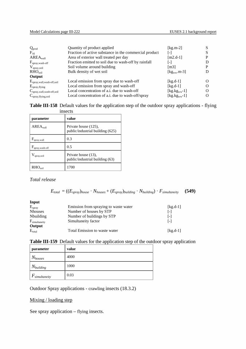
Model Calculations page III-222 EUSES 2.1 background report
Qprod Quantity of product applied [kg.m-2] S FAI Fraction of active substance in the commercial product [-] S AREAwall Area of exterior wall treated per day [m2.d-1] P Fspray,wash-off Fraction emitted to soil due to wash-off by rainfall [-] D Vspray,soil Soil volume around building [m3] P RHOsoil Bulk density of wet soil [kgww.m-3] D Output Espray,wall,wash-off,soil Local emission from spray due to wash-off [kg.d-1] O Espray,flying Local emission from spray and wash-off [kg.d-1] O Cspray,wall,wash-off,soil Local concentration of a.i. due to wash-off [kg.kgww-1] O Cspray,flying,soil Local concentration of a.i. due to wash-off/spray [kg.kgww-1] O Table III-158 Default values for the application step of the outdoor spray applications - flying
insects parameter value
AREAwall Private house (125), public/industrial building (625)
Fspray,wall 0.3
Fspray,wash-off 0.5
Vspray,soil Private house (13), public/industrial building (63)
RHOsoil 1700
Total release
Etotal = ((Espray)house · Nhouses + (Espray)building · Nbuilding) · Fsimultaneity (549) Input Espray Emission from spraying to waste water [kg.d-1] Nhouses Number of houses by STP [-] Nbuilding Number of buildings by STP [-] Fsimultaneity Simultaneity factor [-] Output Etotal Total Emission to waste water [kg.d-1] Table III-159 Default values for the application step of the outdoor spray application parameter value
Nhouses 4000
Nbuilding 1000
Fsimultaneity 0.03
Outdoor Spray applications - crawling insects (18.3.2) Mixing / loading step See spray application – flying insects.
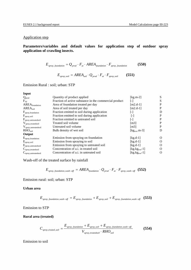
EUSES 2.1 background report Model Calculations page III-223
Application step Parameters/variables and default values for application step of outdoor spray application of crawling insects.
foundationsprayfoundationaiprodfoundationspray FAREAFQE ,, ⋅⋅⋅= (550)
soilsprayaiprodsoilsoilspray FFQAREAE ,, ⋅⋅⋅= (551) Emission Rural : soil; urban: STP Input Qprod Quantity of product applied [kg.m-2] S FAI Fraction of active substance in the commercial product [-] S AREAfoundation Area of foundation treated per day [m2.d-1] P AREAsoil Area of soil treated per day [m2.d-1] P Fspray,foundation Fraction emitted to soil during application [-] D Fspray,soil Fraction emitted to soil during application [-] P Fspray,untreatedsoil Fraction emitted to untreated soil [-] P Vspray,treatedsoil Treated soil volume [m3] P Vspray,untreatedsoil Untreated soil volume [m3] P RHOsoil Bulk density of wet soil [kgww.m-3] D Output Espray,foundation Emission from spraying on foundation [kg.d-1] O Espray,soil Emission from spraying to soil [kg.d-1] O Espray,untreatedsoil Emission from spraying to untreated soil [kg.d-1] O Cspray,treatedsoil Concentration of a.i. in treated soil [kg.kgww-1] O Cspray,untreatedsoil Concentration of a.i. in untreated soil [kg.kgww-1] O Wash-off of the treated surface by rainfall
offwashsprayaiprodfoundationoffwashfoundationspray FFQAREAE −− ⋅⋅⋅= ,,, (552) Emission rural: soil; urban: STP Urban area
offwashfoundationspraysoilsprayfoundationsprayoffwashfoundationspray EEEE −− ++= ,,,,,, (553) Emission to STP Rural area (treated)
soilltreatedsoispray
offwashfoundationspraysoilsprayfoundationspraysoiltreatedspray RHOV
EEEC
⋅
++= −
,
,,,,,, (554)
Emission to soil
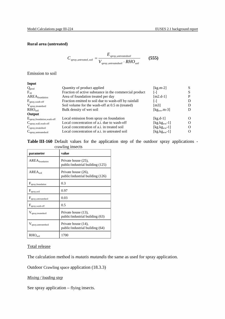
Model Calculations page III-224 EUSES 2.1 background report
Rural area (untreated)
soiloiluntreatedsspray
oiluntreatedsspraysoiluntreatedspray RHOV
EC
⋅=
,
,,, (555)
Emission to soil Input Qprod Quantity of product applied [kg.m-2] S FAI Fraction of active substance in the commercial product [-] S AREAfoundation Area of foundation treated per day [m2.d-1] P Fspray,wash-off Fraction emitted to soil due to wash-off by rainfall [-] D Vspray,treatedsoil Soil volume for the wash-off at 0.5 m (treated) [m3] D RHOsoil Bulk density of wet soil [kgww.m-3] D Output Espray,foundation,wash-off Local emission from spray on foundation [kg.d-1] O Cspray,wall,wash-off Local concentration of a.i. due to wash-off [kg.kgww-1] O Cspray,treatedsoil Local concentration of a.i. in treated soil [kg.kgww-1] O Cspray,untreatedsoil Local concentration of a.i. in untreated soil [kg.kgww-1] O Table III-160 Default values for the application step of the outdoor spray applications -
crawling insects parameter value
AREAfoundation Private house (25), public/industrial building (125)
AREAsoil Private house (26), public/industrial building (126)
Fspray,foundation 0.3
Fspray,soil 0.97
Fspray,untreatedsoil 0.03
Fspray,wash-off 0.5
Vspray,treatedsoil Private house (13), public/industrial building (63)
Vspray,untreatedsoil Private house (14), public/industrial building (64)
RHOsoil 1700
Total release The calculation method is mutatis mutandis the same as used for spray application. Outdoor Crawling space application (18.3.3) Mixing / loading step See spray application – flying insects.
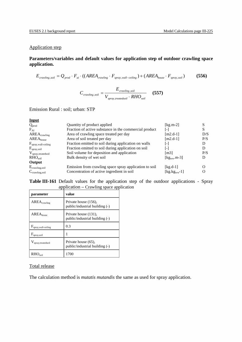
EUSES 2.1 background report Model Calculations page III-225
Application step Parameters/variables and default values for application step of outdoor crawling space application.
)()(( ,,, soilsprayhouseceilingwallspraycrawlingaiprodsoilcrawling FAREAFAREAFQE ⋅+⋅⋅⋅= − (556)
soilltreatedsoispray
soilcrawlingsoilcrawling RHOV
EC
⋅=
,
,, (557)
Emission Rural : soil; urban: STP Input Qprod Quantity of product applied [kg.m-2] S FAI Fraction of active substance in the commercial product [-] S AREAcrawling Area of crawling space treated per day [m2.d-1] D/S AREAhouse Area of soil treated per day [m2.d-1] P/S Fspray,wall-ceiling Fraction emitted to soil during application on walls [-] D Fspray,soil Fraction emitted to soil during application on soil [-] D Vspray,treatedsoil Soil volume for deposition and application [m3] P/S RHOsoil Bulk density of wet soil [kgww.m-3] D Output Ecrawling,soil Emission from crawling space spray application to soil [kg.d-1] O Ccrawling,soil Concentration of active ingredient in soil [kg.kgww-1] O Table III-161 Default values for the application step of the outdoor applications - Spray
application – Crawling space application parameter value
AREAcrawling Private house (156), public/industrial building (-)
AREAhouse Private house (131), public/industrial building (-)
Fspray,wall-ceiling 0.3
Fspray,soil 1
Vspray,treatedsoil Private house (65), public/industrial building (-)
RHOsoil 1700
Total release The calculation method is mutatis mutandis the same as used for spray application.
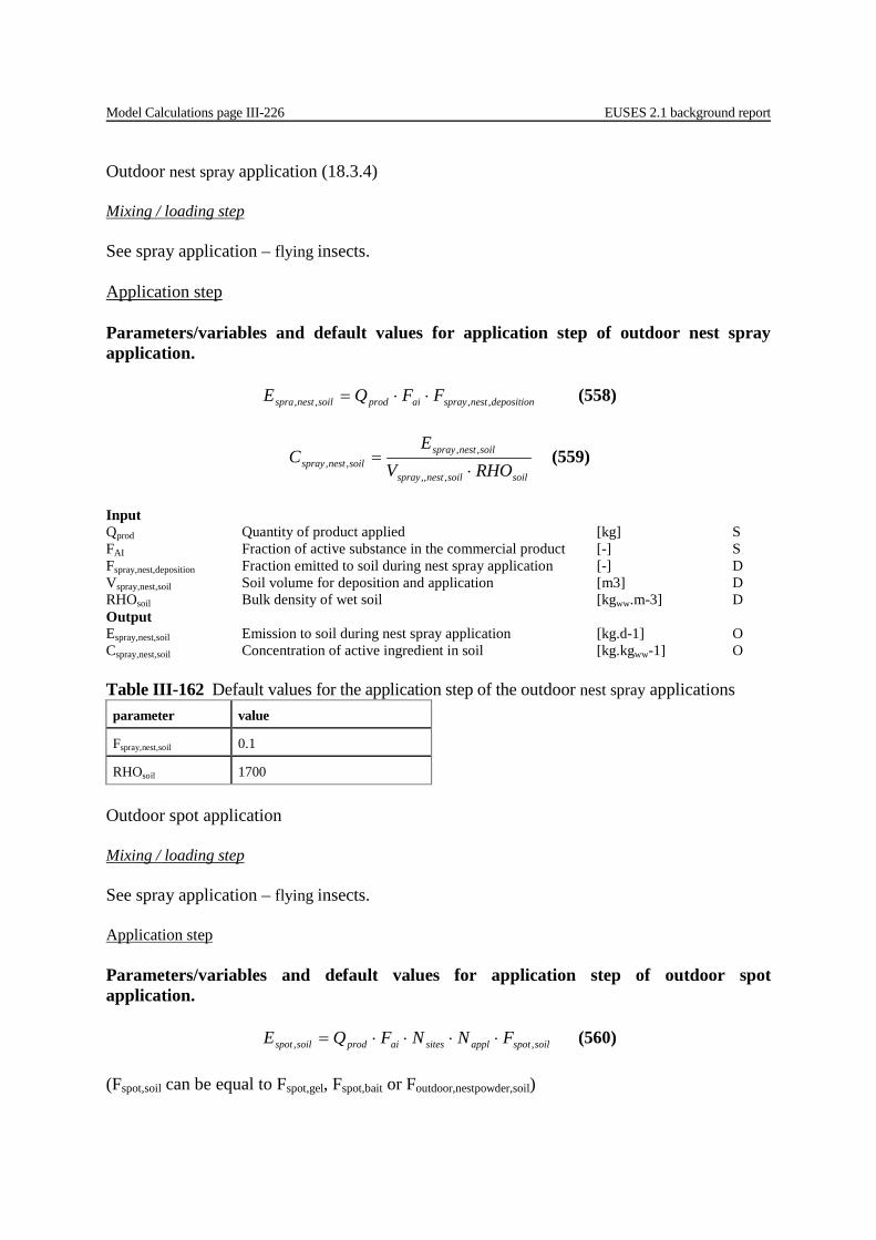
Model Calculations page III-226 EUSES 2.1 background report
Outdoor nest spray application (18.3.4) Mixing / loading step See spray application – flying insects. Application step Parameters/variables and default values for application step of outdoor nest spray application.
depositionnestsprayaiprodsoilnestspra FFQE ,,,, ⋅⋅= (558)
soilsoilnestspray
soilnestspraysoilnestspray RHOV
EC
⋅=
,,,
,,,, (559)
Input Qprod Quantity of product applied [kg] S FAI Fraction of active substance in the commercial product [-] S Fspray,nest,deposition Fraction emitted to soil during nest spray application [-] D Vspray,nest,soil Soil volume for deposition and application [m3] D RHOsoil Bulk density of wet soil [kgww.m-3] D Output Espray,nest,soil Emission to soil during nest spray application [kg.d-1] O Cspray,nest,soil Concentration of active ingredient in soil [kg.kgww-1] O Table III-162 Default values for the application step of the outdoor nest spray applications parameter value
Fspray,nest,soil 0.1
RHOsoil 1700
Outdoor spot application Mixing / loading step See spray application – flying insects. Application step Parameters/variables and default values for application step of outdoor spot application.
soilspotapplsitesaiprodsoilspot FNNFQE ,, ⋅⋅⋅⋅= (560) (Fspot,soil can be equal to Fspot,gel, Fspot,bait or Foutdoor,nestpowder,soil)

EUSES 2.1 background report Model Calculations page III-227
soilsoilosed
soilspotsoilspot RHODEPTHAREA
EC
⋅⋅=
exp
,, (561)
Input Qprod Quantity of product applied [g] S FAI Fraction of active substance in the commercial product [-] S Nsites Number of application sites [-] S Nappl Number of applications [-] S Fspot,gel Fraction emitted to STP during outdoor gel application [-] D Fspot,bait Fraction emitted to STP during outdoor bait application [-] D Foutdoor,nestpowder,soil Fraction emitted to STP during powder application [-] D AREAexposed Area directly exposed to insecticide [m2] D/S DEPTHsoil Depth of exposed soil [m] D VOLUMEsoil Volume of exposed soil [m3] D/S RHOsoil Bulk density of wet soil [kg.m-3] D Output Espot,soil Direct emission rate of a.i. to soil from a campaign [g] O Espot,air Direct emission rate of a.i. to air from a campaign [g] O Cspot,soil Local concentration in soil due to release after a campaign [mg.kg-1] O Table III-163 Default values for the application step of the outdoor spot application parameter value
Fspot,gel 0.9
Fspot,bait 0.2
Foutdoor,nestpowder,soil 0.9
AREAexposed Single point of release (0.25), other (-)
DEPTHsoil 0.5
VOLUMEsoil Single point of release (0.125), other (-)
RHOsoil 1700
Total release The calculation method is mutatis mutandis the same as used for spray application. Secondary poisoning Parameters/variables and default values for the estimated daily intake calculations for the risk assessment of exposure of contaminated food to predators
APPLground = Qprod * FAI (562)
4, 1015.1)/( ⋅⋅⋅⋅= groundcrwalingacute APPLRUDbwFIRETE (563)
4
,sec, 105.2)/( ⋅⋅⋅⋅=− groundmeanflyingtivorousintermshort APPLRUDbwFIRETE (564)
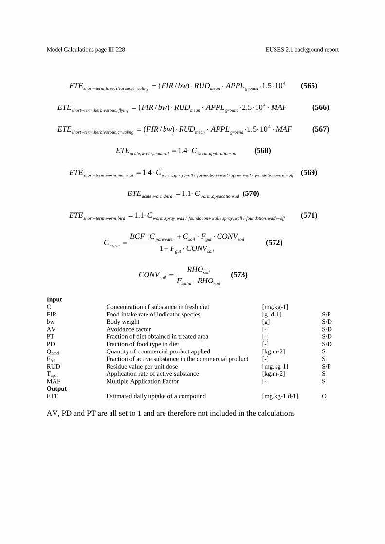
Model Calculations page III-228 EUSES 2.1 background report
4
,sec, 105.1)/( ⋅⋅⋅⋅=− groundmeancrwalingtivorousintermshort APPLRUDbwFIRETE (565)
MAFAPPLRUDbwFIRETE groundmeanflyingsherbivoroutermshort ⋅⋅⋅⋅⋅=−4
,, 105.2)/( (566)
MAFAPPLRUDbwFIRETE groundmeancrwalingsherbivoroutermshort ⋅⋅⋅⋅⋅=−4
,, 105.1)/( (567)
nsoilapplicatiowormmammalwormacute CETE ,,, 4.1 ⋅= (568)
offwashfoundationwallspraywallfoundationwallspraywormmammalwormtermshort CETE −+− ⋅= ,/,//,,,, 4.1 (569)
nsoilapplicatiowormbirdwormacute CETE ,,, 1.1 ⋅= (570)
offwashfoundationwallspraywallfoundationwallspraywormbirdwormtermshort CETE −+− ⋅= ,/,//,,,, 1.1 (571)
soilgut
soilgutsoilporewaterworm CONVF
CONVFCCBCFC
⋅+
⋅⋅+⋅=
1 (572)
soilsoilid
soilsoil RHOF
RHOCONV
⋅= (573)
Input C Concentration of substance in fresh diet [mg.kg-1] FIR Food intake rate of indicator species [g .d-1] S/P bw Body weight [g] S/D AV Avoidance factor [-] S/D PT Fraction of diet obtained in treated area [-] S/D PD Fraction of food type in diet [-] S/D Qprod Quantity of commercial product applied [kg.m-2] S FAI Fraction of active substance in the commercial product [-] S RUD Residue value per unit dose [mg.kg-1] S/P Tappl Application rate of active substance [kg.m-2] S MAF Multiple Application Factor [-] S Output ETE Estimated daily uptake of a compound [mg.kg-1.d-1] O AV, PD and PT are all set to 1 and are therefore not included in the calculations
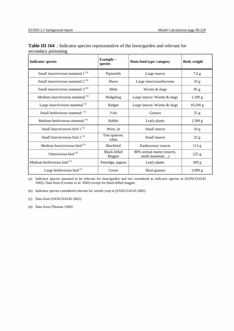
EUSES 2.1 background report Model Calculations page III-229
Table III-164 : Indicator species representative of the lawn/garden and relevant for secondary poisoning
Indicator species Example – species Main food type/ category Body weight
Small insectivorous mammal 1 (a) Pipistrelle Large insects 7.6 g
Small insectivorous mammal 2 (b) Shrew Large insects/earthworms 10 g
Small insectivorous mammal 3 (a) Mole Worms & slugs 85 g
Medium insectivorous mammal (a) Hedgehog Large insects/ Worms & slugs 1,100 g
Large insectivorous mammal (a) Badger Large insects/ Worms & slugs 10,100 g
Small herbivorous mammal (c) Vole Grasses 25 g
Medium herbivorous mammal (a) Rabbit Leafy plants 1,500 g
Small Insectivorous bird 1 (c) Wren, tit Small insects 10 g
Small Insectivorous bird 2 (a) Tree sparrow, robin Small insects 22 g
Medium Insectivorous bird (a) Blackbird Earthworms/ insects 113 g
Omnivorous bird (d) Black-billed Magpie
80% animal matter (insects, small mammals…) 225 g
Medium herbivorous bird (c) Partridge, pigeon Leafy plants 300 g
Large herbivorous bird (c) Goose Short grasses 3,000 g
(a) Indicator species assumed to be relevant for lawn/garden and not considered as indicator species in (SANCO/4145 2002). Data from (Crocker et al. 2002) except for black-billed magpie.
(b) Indicator species considered relevant for cereals crop in (SANCO/4145 2002)
(c) Data from (SANCO/4145 2002)
(d) Data from (Thomas 1994)
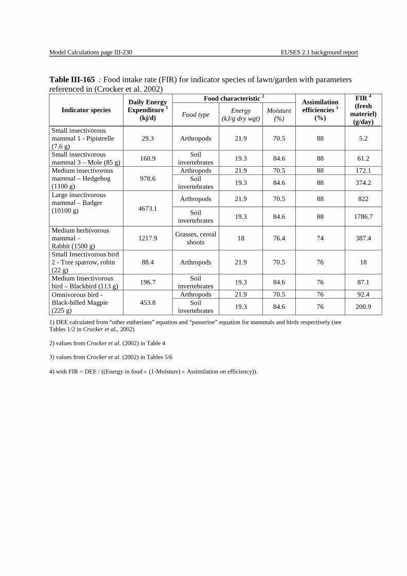
Model Calculations page III-230 EUSES 2.1 background report
Table III-165 : Food intake rate (FIR) for indicator species of lawn/garden with parameters referenced in (Crocker et al. 2002)
Indicator species Daily Energy Expenditure 1
(kj/d)
Food characteristic 2 Assimilation efficiencies 3
(%)
FIR 4
(fresh materiel) (g/day)
Food type Energy (kJ/g dry wgt)
Moisture (%)
Small insectivorous mammal 1 - Pipistrelle (7.6 g)
29.3 Arthropods 21.9 70.5 88 5.2
Small insectivorous mammal 3 – Mole (85 g) 160.9 Soil
invertebrates 19.3 84.6 88 61.2
Medium insectivorous mammal – Hedgehog (1100 g)
978.6 Arthropods 21.9 70.5 88 172.1
Soil invertebrates 19.3 84.6 88 374.2
Large insectivorous mammal – Badger (10100 g) 4673.1
Arthropods 21.9 70.5 88 822
Soil invertebrates 19.3 84.6 88 1786.7
Medium herbivorous mammal – Rabbit (1500 g)
1217.9 Grasses, cereal shoots 18 76.4 74 387.4
Small Insectivorous bird 2 - Tree sparrow, robin (22 g)
88.4 Arthropods 21.9 70.5 76 18
Medium Insectivorous bird – Blackbird (113 g) 196.7 Soil
invertebrates 19.3 84.6 76 87.1
Omnivorous bird - Black-billed Magpie (225 g)
453.8 Arthropods 21.9 70.5 76 92.4
Soil invertebrates 19.3 84.6 76 200.9
1) DEE calculated from “other eutherians” equation and “passerine” equation for mammals and birds respectively (see Tables 1/2 in Crocker et al., 2002)
2) values from Crocker et al. (2002) in Table 4
3) values from Crocker et al. (2002) in Tables 5/6
4) with FIR = DEE / ((Energy in food × (1-Moisture) × Assimilation on efficiency)).
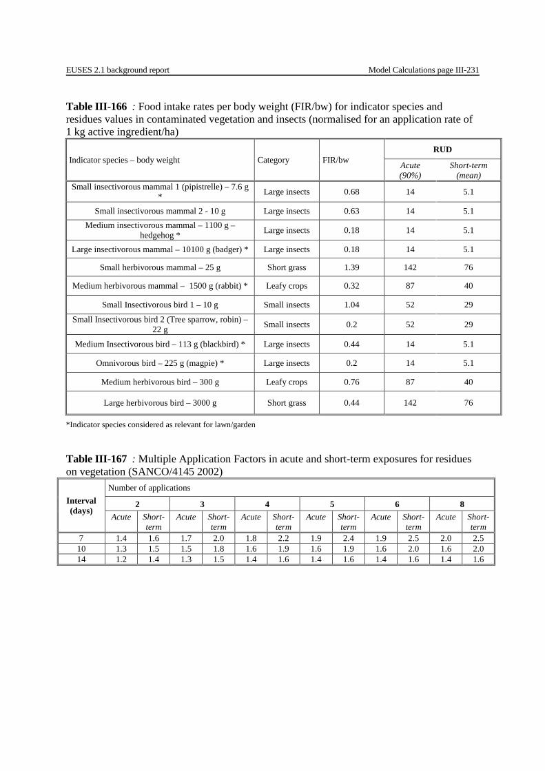
EUSES 2.1 background report Model Calculations page III-231
Table III-166 : Food intake rates per body weight (FIR/bw) for indicator species and residues values in contaminated vegetation and insects (normalised for an application rate of 1 kg active ingredient/ha)
Indicator species – body weight Category FIR/bw RUD
Acute (90%)
Short-term (mean)
Small insectivorous mammal 1 (pipistrelle) – 7.6 g * Large insects 0.68 14 5.1
Small insectivorous mammal 2 - 10 g Large insects 0.63 14 5.1 Medium insectivorous mammal – 1100 g –
hedgehog * Large insects 0.18 14 5.1
Large insectivorous mammal – 10100 g (badger) * Large insects 0.18 14 5.1
Small herbivorous mammal – 25 g Short grass 1.39 142 76
Medium herbivorous mammal – 1500 g (rabbit) * Leafy crops 0.32 87 40
Small Insectivorous bird 1 – 10 g Small insects 1.04 52 29
Small Insectivorous bird 2 (Tree sparrow, robin) – 22 g Small insects 0.2 52 29
Medium Insectivorous bird – 113 g (blackbird) * Large insects 0.44 14 5.1
Omnivorous bird – 225 g (magpie) * Large insects 0.2 14 5.1
Medium herbivorous bird – 300 g Leafy crops 0.76 87 40
Large herbivorous bird – 3000 g Short grass 0.44 142 76
*Indicator species considered as relevant for lawn/garden
Table III-167 : Multiple Application Factors in acute and short-term exposures for residues on vegetation (SANCO/4145 2002)
Interval (days)
Number of applications
2 3 4 5 6 8 Acute Short-
term Acute Short-
term Acute Short-
term Acute Short-
term Acute Short-
term Acute Short-
term 7 1.4 1.6 1.7 2.0 1.8 2.2 1.9 2.4 1.9 2.5 2.0 2.5 10 1.3 1.5 1.5 1.8 1.6 1.9 1.6 1.9 1.6 2.0 1.6 2.0 14 1.2 1.4 1.3 1.5 1.4 1.6 1.4 1.6 1.4 1.6 1.4 1.6

Model Calculations page III-232 EUSES 2.1 background report
III.3.6.15 Product type 21: Antifouling products The scenarios and models and calculation formulations used in this version of EUSES 2.1.1 for antifouling products have been taken from the following document:
− Harmonisation of Environmental Emission Scenarios: An Emission Scenario Document for Antifouling Products in OECD countries. (EC, Directorate-General Environment, 2004)
This document can be obtained from the ECB Biocides website The following additions are made: The ESD provides formulas to calculate the total emissions to the different compartments only, but not to calculate the concentrations. In the present EUSES 2.1.1 version formulas are implemented taken into account the possibility for (bio)degradation and using the dimensions given in the ESD. These formulas are based on those given in the USES 2.0 documentation, section III 4.9.1 and 4.8.16 (Linders and Jagers, 1998). .3.5.3. Antifouling The following scenarios for calculation the concentration in different environmental compartments for the application and removal of compounds used as antifoulings can be distinguished: New building
• Commercial ships professional (scenario 1); • Pleasure craft professional. (scenario 2)
Maintenance and repair
• Commercial ships professional (scenario 3); • Pleasure craft professional (scenario 4);
non-professional (scenario 5). The scenarios for new building are related to the application of an antifouling paint only. Removal of the old paint layer on a ship hull takes place only during M&R of ship hulls after which a new paint will be applied. It is considered that application and removal for the maintenance and repair occur within the same time frame and at the same site. Therefore, the emissions from application and removal have to be linked to one other. With respect to the emission to soil this means that the calculated PECs will be summed up. With respect to the release to STP and/or water, the PECs can be treated separately, assuming that the time between application and removal is long enough for a total dissipation/dilution. For most of the scenario the direct emission is restricted to one or two compartments: New building
• Commercial ships professional water • Pleasure craft professional. soil, STP

EUSES 2.1 background report Model Calculations page III-233
Maintenance and repair
• Commercial ships professional; water • Pleasure craft professional; soil, STP (and water at removal only)
non-professional. soil, STP (and water at removal only) Overview of the timeframe for application and removal of paint Application New building ships (emission to water) Tfreq = 2 (2 days per year a ship will be painted) Tpaint = 1 day Tpaint = 1 day Nboat = 1 Nboat = 1 The PEC in water and sediment (via EP) will be calculated on a daily base both for a river and a harbour. New building pleasure craft (emission to soil and STP) Realistic worst case: Tfreq = 30 with regular intervals (Total painting days = 2 * 30 days) Typical case is different: Tpaint = 365 and Nboat = 300, hence all most every days a pleasure craft is painted. However, according to the ESD there is no emission. Tpaint = 2 days Nboat = 1 The concentration in water and sediment (via EP) resulting from the release to a STP will be calculated on a daily base. The concentration in sludge will be divided by 6.1 (=365/60) to calculate a yearly average sludge concentration. The concentration in soil will be calculated using the equations 1 -6, where Csoil 0-paint is based on two paint days.

Model Calculations page III-234 EUSES 2.1 background report
Application of paint and removal M&R ships (emission to water) Realistic worst case and typical case: Tfreq = 20 with regular intervals (Total painting days = 2 * 20 days) Tpaint = 2 days Tremoval = 1 day Nboat = 1 The PEC in water and sediment (via EP) in a harbour will be calculated based on two painting days and 1 removal day, taking into account removal process between these events (see P-8) It is assumed that the interval between the different painting + removal events is long enough that no accumulation is to be expected. The PEC water and sediment in a river will be calculated on a daily base. M&R pleasure craft (prof) (emission to soil and STP+ water with respect to removal) The calculated Elocal to soil and STP are daily emissions during a period of 183 days, after which no activities take place during 183 days (Total painting days = 183 days)
Tpaint = 183 days Tint = 183 days The concentration in water and sediment (via EP) resulting from the release to a STP will be calculated on a daily base. As the release is continuous no deviation from the standard calculation of the concentration in sludge is necessary. The concentration in sludge for application and removal has to be added. The concentration in soil will be calculated using the equations 1 -6, where Csoil 0-paint is based on a daily release. M&R pleasure craft (non-prof) (emission to soil and STP+ water with respect to removal) At this scenario 5 boats are painted within a period of 91 days with regular intervals (Tinterval = 91/(5-1)= 22.5 days). Total painting days = 1 * 5 days For removal there are two scenarios typical and realistic worst case. For typical case the same scenario is used as for application. For realistic worst case every day (during 91 days) paint is removed. Tpaint = 91 days Tint = 274 days Nboat = 5
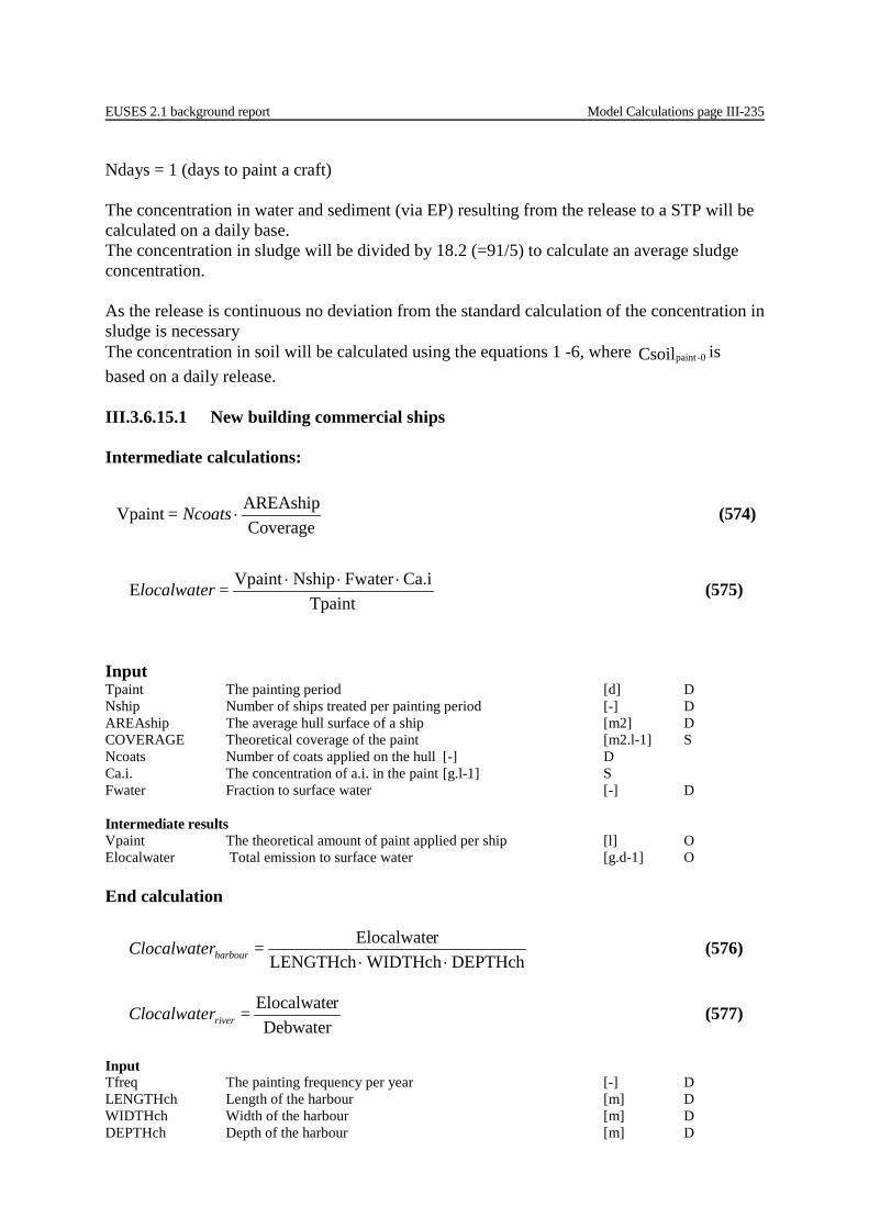
EUSES 2.1 background report Model Calculations page III-235
Ndays = 1 (days to paint a craft) The concentration in water and sediment (via EP) resulting from the release to a STP will be calculated on a daily base. The concentration in sludge will be divided by 18.2 (=91/5) to calculate an average sludge concentration. As the release is continuous no deviation from the standard calculation of the concentration in sludge is necessary The concentration in soil will be calculated using the equations 1 -6, where Csoil 0-paint is based on a daily release. III.3.6.15.1 New building commercial ships
Intermediate calculations:
Input Tpaint The painting period [d] D Nship Number of ships treated per painting period [-] D AREAship The average hull surface of a ship [m2] D COVERAGE Theoretical coverage of the paint [m2.l-1] S Ncoats Number of coats applied on the hull [-] D Ca.i. The concentration of a.i. in the paint [g.l-1] S Fwater Fraction to surface water [-] D Intermediate results Vpaint The theoretical amount of paint applied per ship [l] O Elocalwater Total emission to surface water [g.d-1] O End calculation
= rClocalwate harbour DEPTHchWIDTHchLENGTHchrElocalwate⋅⋅
(576)
= rClocalwate river DebwaterrElocalwate (577)
Input Tfreq The painting frequency per year [-] D LENGTHch Length of the harbour [m] D WIDTHch Width of the harbour [m] D DEPTHch Depth of the harbour [m] D
Ncoats = Coverage
AREAshipVpaint ⋅ (574)
= localwaterTpaint
Ca.iFwaterNshipVpaintE ⋅⋅⋅ (575)
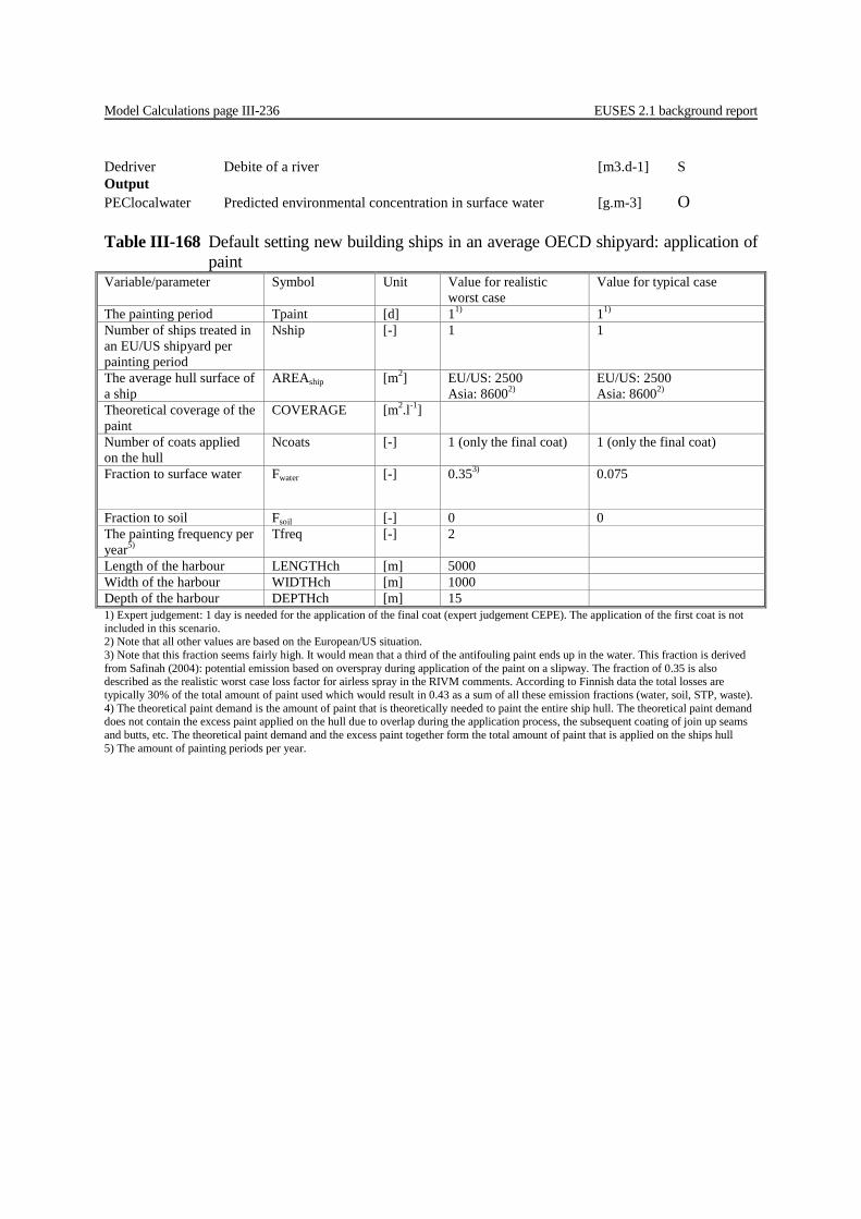
Model Calculations page III-236 EUSES 2.1 background report
Dedriver Debite of a river [m3.d-1] S Output PEClocalwater Predicted environmental concentration in surface water [g.m-3] O Table III-168 Default setting new building ships in an average OECD shipyard: application of
paint Variable/parameter Symbol Unit Value for realistic
worst case Value for typical case
The painting period Tpaint [d] 11) 11) Number of ships treated in an EU/US shipyard per painting period
Nship [-] 1 1
The average hull surface of a ship
AREAship [m2] EU/US: 2500 Asia: 86002)
EU/US: 2500 Asia: 86002)
Theoretical coverage of the paint
COVERAGE [m2.l-1]
Number of coats applied on the hull
Ncoats [-] 1 (only the final coat) 1 (only the final coat)
Fraction to surface water Fwater [-] 0.353) 0.075
Fraction to soil Fsoil [-] 0 0 The painting frequency per year5)
Tfreq [-] 2
Length of the harbour LENGTHch [m] 5000 Width of the harbour WIDTHch [m] 1000 Depth of the harbour DEPTHch [m] 15 1) Expert judgement: 1 day is needed for the application of the final coat (expert judgement CEPE). The application of the first coat is not included in this scenario. 2) Note that all other values are based on the European/US situation. 3) Note that this fraction seems fairly high. It would mean that a third of the antifouling paint ends up in the water. This fraction is derived from Safinah (2004): potential emission based on overspray during application of the paint on a slipway. The fraction of 0.35 is also described as the realistic worst case loss factor for airless spray in the RIVM comments. According to Finnish data the total losses are typically 30% of the total amount of paint used which would result in 0.43 as a sum of all these emission fractions (water, soil, STP, waste). 4) The theoretical paint demand is the amount of paint that is theoretically needed to paint the entire ship hull. The theoretical paint demand does not contain the excess paint applied on the hull due to overlap during the application process, the subsequent coating of join up seams and butts, etc. The theoretical paint demand and the excess paint together form the total amount of paint that is applied on the ships hull 5) The amount of painting periods per year.
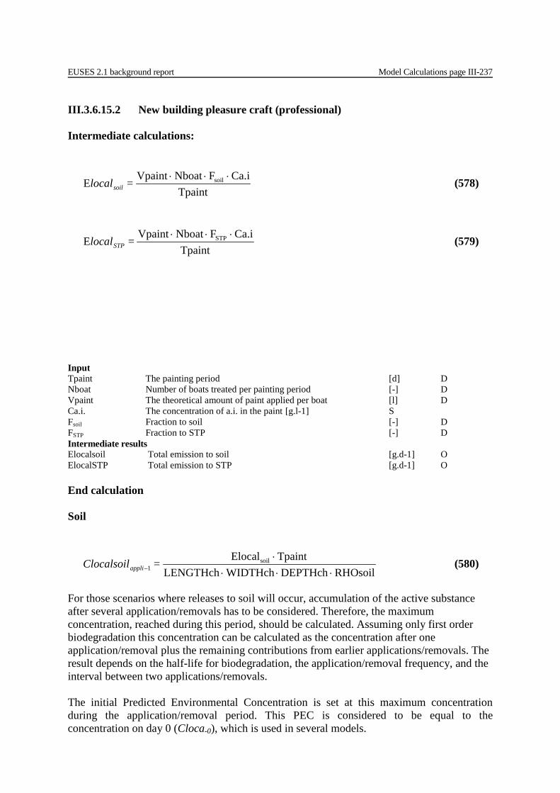
EUSES 2.1 background report Model Calculations page III-237
III.3.6.15.2 New building pleasure craft (professional) Intermediate calculations:
= localsoil TpaintCa.iFNboatVpaint
E soil ⋅⋅⋅ (578)
= localSTP TpaintCa.iFNboatVpaint
E STP ⋅⋅⋅ (579)
Input Tpaint The painting period [d] D Nboat Number of boats treated per painting period [-] D Vpaint The theoretical amount of paint applied per boat [l] D Ca.i. The concentration of a.i. in the paint [g.l-1] S Fsoil Fraction to soil [-] D FSTP Fraction to STP [-] D Intermediate results Elocalsoil Total emission to soil [g.d-1] O ElocalSTP Total emission to STP [g.d-1] O End calculation Soil
= Clocalsoilappli RHOsoilDEPTHchWIDTHchLENGTHchTpaintElocalsoil
1 ⋅⋅⋅⋅
− (580)
For those scenarios where releases to soil will occur, accumulation of the active substance after several application/removals has to be considered. Therefore, the maximum concentration, reached during this period, should be calculated. Assuming only first order biodegradation this concentration can be calculated as the concentration after one application/removal plus the remaining contributions from earlier applications/removals. The result depends on the half-life for biodegradation, the application/removal frequency, and the interval between two applications/removals. The initial Predicted Environmental Concentration is set at this maximum concentration during the application/removal period. This PEC is considered to be equal to the concentration on day 0 (Cloca-0), which is used in several models.

Model Calculations page III-238 EUSES 2.1 background report
Input LENGTHch Length of the soil [m] D WIDTHch Width of the soil [m] D DEPTHch Depth of the soil [m] D RHOsoildwt Soil density (dry weight) [kg.m-3] D Csoilpaint-1 appl concentration in soil after one application/removal [kgc.kgwwt
-1] O kdegsoil rate constant for degradation in soil [d-1] O Nappl number of applications/removal in one year [-] D Frs fraction of the concentration remaining after time Tinterval [-] Oc Tinterval application interval [d] D Tpaint the painting period [d] D Tfreq the painting frequency per year [-] D Output Csoilpaint-0 peak concentration in soil after N applications [kgc.kgwwt
-1] O Csoilpaint-T average in soil concentration over T days [kgc.kgwwt
-1] O PECs for soil, long-term application The PEC after long-term application is set at the concentration after the last application/removal in the tenth year. This PEC is considered to be equal to the soil concentration at year 10 (Csoilpaint-0,lt). After the tenth year the resulting concentration, Csoilpaint-lt, is compared to the PNEC.
intervalTkdeg -rs
soile= F ⋅ (581)
1
int/int
−freq
removalpaerval T
T= T
rs
Nrs
appl/remov
1) - N(rsappl/remov
2rsappl/remov
rsappl/removappl/remov 0-alappl/remov
F- 1 F- 1
Csoil =
F Csoil + ... + F Csoil
+ F Csoil + Csoil = Csoil
appl
appl/remov
⋅
⋅⋅
⋅
(582)
)T-(365 kdeg -0-paint1 -paint
paintsoileCsoil = Csoil ⋅⋅ (583)
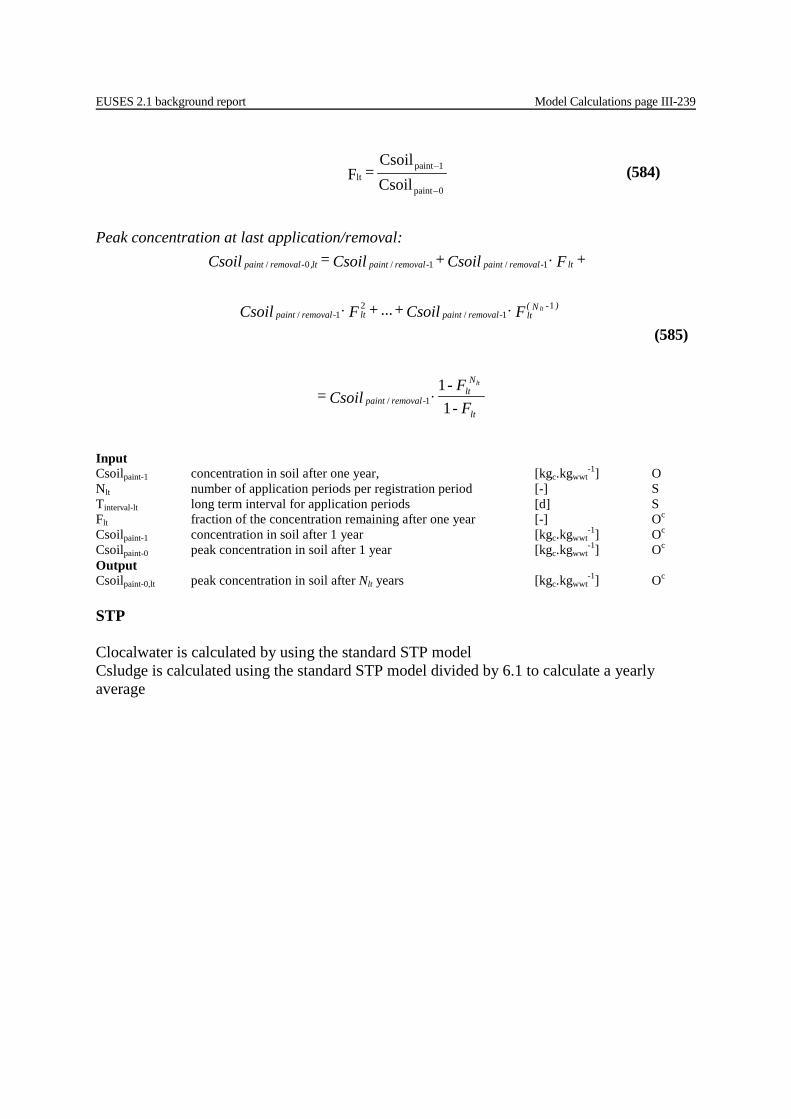
EUSES 2.1 background report Model Calculations page III-239
Peak concentration at last application/removal:
Input Csoilpaint-1 concentration in soil after one year, [kgc.kgwwt
-1] O Nlt number of application periods per registration period [-] S Tinterval-lt long term interval for application periods [d] S Flt fraction of the concentration remaining after one year [-] Oc Csoilpaint-1 concentration in soil after 1 year [kgc.kgwwt
-1] Oc
Csoilpaint-0 peak concentration in soil after 1 year [kgc.kgwwt-1] Oc
Output Csoilpaint-0,lt peak concentration in soil after Nlt years [kgc.kgwwt
-1] Oc STP Clocalwater is calculated by using the standard STP model Csludge is calculated using the standard STP model divided by 6.1 to calculate a yearly average
0paint
1paintlt Csoil
Csoil = F
−
− (584)
lt
Nlt
-removalpaint
) - N(lt-removalpaintlt-removalpaint
lt-removalpaint-removalpaintlt,-removalpaint
F- F-
Csoil =
F Csoil + ... + F Csoil
+ F Csoil + Csoil = Csoil
lt
lt
11
1/
11/
21/
1/1/0/
⋅
⋅⋅
⋅
(585)

Model Calculations page III-240 EUSES 2.1 background report
Table III-169 New building pleasure craft in an average OECD boatyard: application of paint Variable/parameter Symbol Unit Value for realistic worst
case Value for typical case
The painting period Tpaint [d] 2 365 Number of boats treated in a boatyard per painting period
Nboat [-] 1 300
The concentration of active ingredient in the paint
Ca.i. [g.l-1]
The theoretical amount of paint applied per boat1)
Vpaint [l] 3 3
Fraction to surface water Fwater [-] 0 0 Fraction to STP2)
FSTP [-] Application by mixture of
airless spray / brush and roller: Max. 0.06 Application by brush and roller only: Max. 0.025
0
Fraction to soil2)
Fsoil [-] Application by mixture of airless spray / brush and roller: Max. 0.06 Application by brush and roller only: Max. 0.025
0
The painting frequency per year Tfreq [-] Realistic worst case: 30 Typical case: n/a
Length of the receiving soil compartment3)
LENGTH [m] 9.5 9.5
Width of the receiving soil compartment
WIDTH [m] 4.5 4.5
Depth of the receiving soil compartment
DEPTH [m] 0.14) 0.14)
Soil density (dry weight) RHOsoildw [kg.m-3] 15045) 15045) 1) The system of paint volume demand is very different to ships. Most of the paint companies assume that the coating will be applied by the boat owner/yard and so supply a paint calculator. Using this calculator the required paint amount can be estimated. However, this is not what happens in practice. In reality the typical owner applies one touch up coat to the existing antifouling coating and one full coat of antifouling. On the basis of discussions with paint companies, boat builders and marina operators etc. Safinah has determined default values for the theoretical amount of paint applied per boat. 2) Depending on the control measurements of the boat yard the emission up to a maximum of 6% (potential emission weighted for brush/roller and spray) or 2.5% (for brush and roller only) either goes to soil or a STP or a mixture between these two options 3) A boat of 7.5 m length and 2.5 m width is assumed. For the determination of the surface of the receiving soil compartment a “walking path” around the boat for the applier of the paint is assumed. It was estimated that this path is 1 metre wide. 4) In line with the environmental emission scenario of the OECD for Wood Preservatives. 5) Based on EU-TGD (ECB, 20034) (wet weight is 1700 kg.m-3). III.3.6.15.3 Maintenance and repair
• Commercial ships professional; Application
Ncoats = Coverage
AREAshipVpaint ⋅ (586)
= localwaterTpaint
Ca.iFwaterNshipVpaintE ⋅⋅⋅ (587)
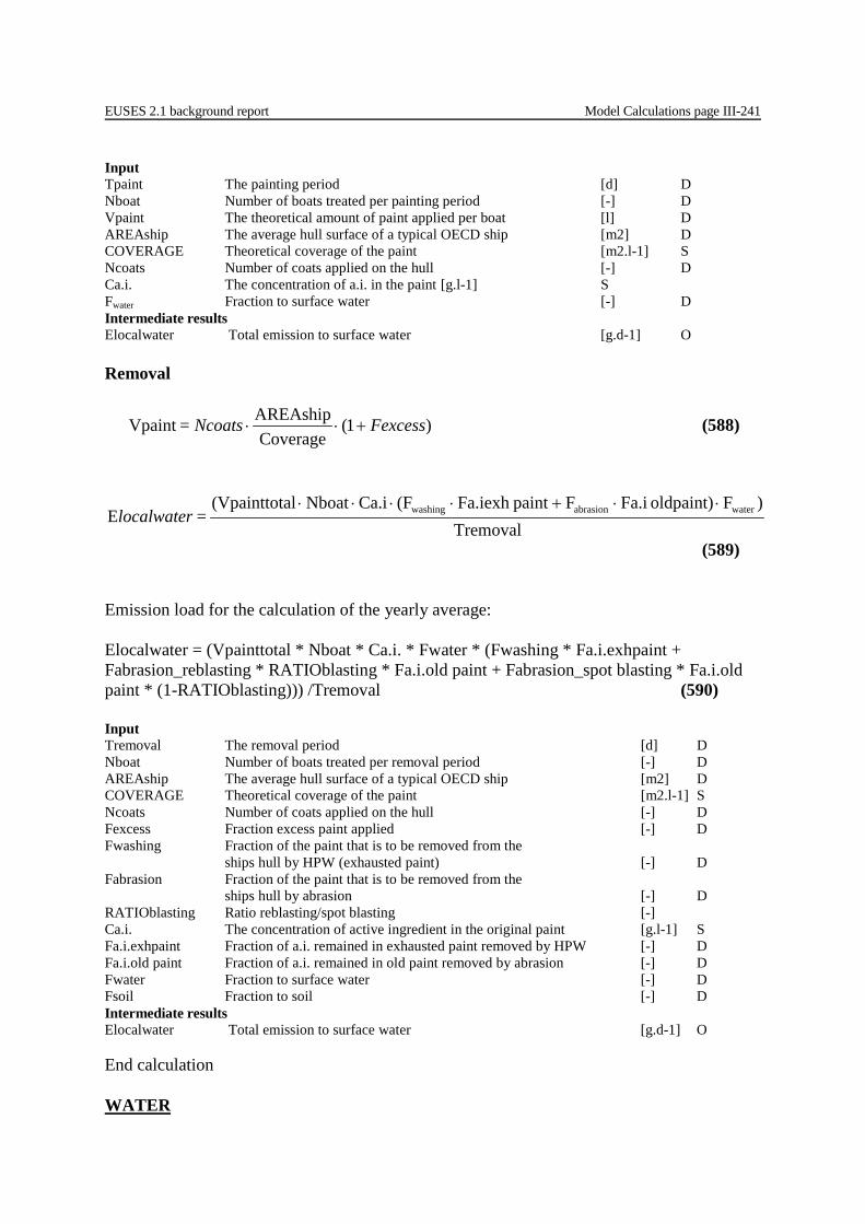
EUSES 2.1 background report Model Calculations page III-241
Input Tpaint The painting period [d] D Nboat Number of boats treated per painting period [-] D Vpaint The theoretical amount of paint applied per boat [l] D AREAship The average hull surface of a typical OECD ship [m2] D COVERAGE Theoretical coverage of the paint [m2.l-1] S Ncoats Number of coats applied on the hull [-] D Ca.i. The concentration of a.i. in the paint [g.l-1] S Fwater Fraction to surface water [-] D Intermediate results Elocalwater Total emission to surface water [g.d-1] O Removal
)1(Coverage
AREAshipVpaint Fexcess Ncoats = +⋅⋅ (588)
= localwaterTremoval
)Foldpaint) Fa.iFpaintFa.iexh (FCa.iNboatal(VpainttotE waterabrasionwashing ⋅⋅+⋅⋅⋅⋅
(589) Emission load for the calculation of the yearly average: Elocalwater = (Vpainttotal * Nboat * Ca.i. * Fwater * (Fwashing * Fa.i.exhpaint + Fabrasion_reblasting * RATIOblasting * Fa.i.old paint + Fabrasion_spot blasting * Fa.i.old paint * (1-RATIOblasting))) /Tremoval (590) Input Tremoval The removal period [d] D Nboat Number of boats treated per removal period [-] D AREAship The average hull surface of a typical OECD ship [m2] D COVERAGE Theoretical coverage of the paint [m2.l-1] S Ncoats Number of coats applied on the hull [-] D Fexcess Fraction excess paint applied [-] D Fwashing Fraction of the paint that is to be removed from the
ships hull by HPW (exhausted paint) [-] D Fabrasion Fraction of the paint that is to be removed from the
ships hull by abrasion [-] D RATIOblasting Ratio reblasting/spot blasting [-] Ca.i. The concentration of active ingredient in the original paint [g.l-1] S Fa.i.exhpaint Fraction of a.i. remained in exhausted paint removed by HPW [-] D Fa.i.old paint Fraction of a.i. remained in old paint removed by abrasion [-] D Fwater Fraction to surface water [-] D Fsoil Fraction to soil [-] D Intermediate results Elocalwater Total emission to surface water [g.d-1] O End calculation WATER

Model Calculations page III-242 EUSES 2.1 background report
Harbour
= rClocalwate removalapplharbour DEPTHchWIDTHchLENGTHchrElocalwate_ / ⋅⋅
(591)
Cwatere Cwatere Cwater= rClocalwate applik
applk
removalharbourbaba +⋅+⋅ ⋅⋅ −− sinsin deg2.deg (592)
River Elocalwater goes directly to surface water. Therefore in EUSES by pass STP should be selected. Here PEC water is calculated for application and removal separately. For the risk assessment the highest PEC is used. Input LENGTHch Length of the harbour [m] D WIDTHch Width of the harbour [m] D DEPTHch Depth of the harbour [m] D FLOWriver Flow rate of a river [m3.d-1] S Output PEClocalwater Predicted environmental concentration in surface water [g.m-3] O parameters required for distribution models
Default for this scenario Unit Value
FLOW FLOWriver [m3.d-1] -
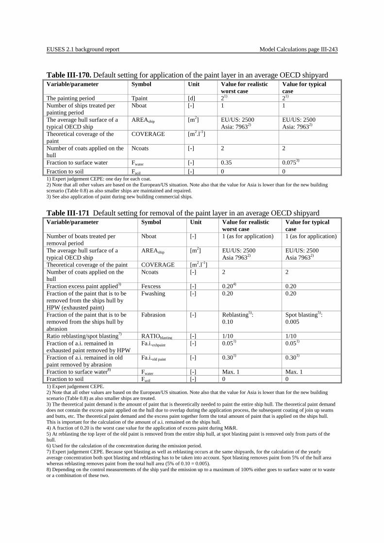
EUSES 2.1 background report Model Calculations page III-243
Table III-170. Default setting for application of the paint layer in an average OECD shipyard Variable/parameter Symbol Unit Value for realistic
worst case Value for typical case
The painting period Tpaint [d] 21) 21) Number of ships treated per painting period
Nboat [-] 1 1
The average hull surface of a typical OECD ship
AREAship [m2] EU/US: 2500 Asia: 79632)
EU/US: 2500 Asia: 79632)
Theoretical coverage of the paint
COVERAGE [m2.l-1]
Number of coats applied on the hull
Ncoats [-] 2 2
Fraction to surface water Fwater [-] 0.35 0.0753) Fraction to soil Fsoil [-] 0 0 1) Expert judgement CEPE: one day for each coat. 2) Note that all other values are based on the European/US situation. Note also that the value for Asia is lower than for the new building scenario (Table 0.8) as also smaller ships are maintained and repaired. 3) See also application of paint during new building commercial ships. Table III-171 Default setting for removal of the paint layer in an average OECD shipyard Variable/parameter Symbol Unit Value for realistic
worst case Value for typical case
Number of boats treated per removal period
Nboat [-] 1 (as for application) 1 (as for application)
The average hull surface of a typical OECD ship
AREAship [m2] EU/US: 2500 Asia 79632)
EU/US: 2500 Asia 79632)
Theoretical coverage of the paint COVERAGE [m2.l-1] Number of coats applied on the hull
Ncoats [-] 2 2
Fraction excess paint applied3) Fexcess [-] 0.204) 0.20 Fraction of the paint that is to be removed from the ships hull by HPW (exhausted paint)
Fwashing [-] 0.20 0.20
Fraction of the paint that is to be removed from the ships hull by abrasion
Fabrasion [-] Reblasting5): 0.10
Spot blasting5): 0.005
Ratio reblasting/spot blasting7) RATIOblasting [-] 1/10 1/10 Fraction of a.i. remained in exhausted paint removed by HPW
Fa.i.exhpaint [-] 0.051) 0.051)
Fraction of a.i. remained in old paint removed by abrasion
Fa.i.old paint [-] 0.301) 0.301)
Fraction to surface water8) Fwater [-] Max. 1 Max. 1 Fraction to soil Fsoil [-] 0 0 1) Expert judgement CEPE. 2) Note that all other values are based on the European/US situation. Note also that the value for Asia is lower than for the new building scenario (Table 0.8) as also smaller ships are treated. 3) The theoretical paint demand is the amount of paint that is theoretically needed to paint the entire ship hull. The theoretical paint demand does not contain the excess paint applied on the hull due to overlap during the application process, the subsequent coating of join up seams and butts, etc. The theoretical paint demand and the excess paint together form the total amount of paint that is applied on the ships hull. This is important for the calculation of the amount of a.i. remained on the ships hull. 4) A fraction of 0.20 is the worst case value for the application of excess paint during M&R. 5) At reblasting the top layer of the old paint is removed from the entire ship hull, at spot blasting paint is removed only from parts of the hull. 6) Used for the calculation of the concentration during the emission period. 7) Expert judgement CEPE. Because spot blasting as well as reblasting occurs at the same shipyards, for the calculation of the yearly average concentration both spot blasting and reblasting has to be taken into account. Spot blasting removes paint from 5% of the hull area whereas reblasting removes paint from the total hull area (5% of 0.10 = 0.005). 8) Depending on the control measurements of the ship yard the emission up to a maximum of 100% either goes to surface water or to waste or a combination of these two.

Model Calculations page III-244 EUSES 2.1 background report
Table III-172 Default settings for the calculation of the environmental concentrations for application and removal of the paint layer during M&R of commercial ships in an average OECD shipyard
Variable/parameter Unit Symbol Value The removal frequency per year1) [-] Tfreq 202) Length of the harbour [m] LENGTHch 5000 Width of the harbour [m] WIDTHch 1000 Depth of the harbour [m] DEPTHch 15 III.3.6.15.4 Professional M&R pleasure craft Application Intermediate calculations:
= localsoil TpaintCa.iFNboatVpaint
E soil ⋅⋅⋅ (593)
= localSTP TpaintCa.iFNboatVpaint
E STP ⋅⋅⋅ (594)
Input Tpaint The painting period [d] D Nboat Number of boats treated per painting period [-] D Vpaint The theoretical amount of paint applied per boat [l] D Ca.i. The concentration of a.i. in the paint [g.l-1] S Fsoil Fraction to soil [-] D FSTP Fraction to STP [-] D Intermediate results Elocalsoil Total emission to soil [g.d-1] O ElocalSTP Total emission to STP [g.d-1] O Removal Intermediate calculation:
= localsoilTremoval
)Foldpaint) Fa.iFpaintFa.iexh (FCa.iNboatal(VpainttotE soilabrasionwashing ⋅⋅+⋅⋅⋅⋅
(595)
= localSTPTremoval
)Foldpaint) Fa.iFpaintFa.iexh (FCa.iNboatal(VpainttotE STPabrasionwashing ⋅⋅+⋅⋅⋅⋅
(596)
= localwaterTremoval
)Foldpaint) Fa.iFpaintFa.iexh (FCa.iNboatal(VpainttotE waterabrasionwashing ⋅⋅+⋅⋅⋅⋅
(597)
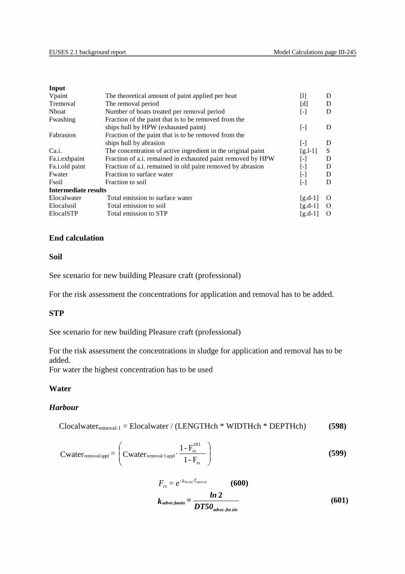
EUSES 2.1 background report Model Calculations page III-245
Input Vpaint The theoretical amount of paint applied per boat [l] D Tremoval The removal period [d] D Nboat Number of boats treated per removal period [-] D Fwashing Fraction of the paint that is to be removed from the
ships hull by HPW (exhausted paint) [-] D Fabrasion Fraction of the paint that is to be removed from the
ships hull by abrasion [-] D Ca.i. The concentration of active ingredient in the original paint [g.l-1] S Fa.i.exhpaint Fraction of a.i. remained in exhausted paint removed by HPW [-] D Fa.i.old paint Fraction of a.i. remained in old paint removed by abrasion [-] D Fwater Fraction to surface water [-] D Fsoil Fraction to soil [-] D Intermediate results Elocalwater Total emission to surface water [g.d-1] O Elocalsoil Total emission to soil [g.d-1] O ElocalSTP Total emission to STP [g.d-1] O End calculation Soil See scenario for new building Pleasure craft (professional) For the risk assessment the concentrations for application and removal has to be added. STP See scenario for new building Pleasure craft (professional) For the risk assessment the concentrations in sludge for application and removal has to be added. For water the highest concentration has to be used Water Harbour
Clocalwaterremoval-1 = Elocalwater / (LENGTHch * WIDTHch * DEPTHch) (598)
⋅
rs
183rs
appl 1removal/ plremoval/ap F- 1 F- 1
Cwater = Cwater (599)
intervalsin Tk -
rsbae= F ⋅ (600)
sinba,advec
basinadvec, DT50 ln= k2 (601)
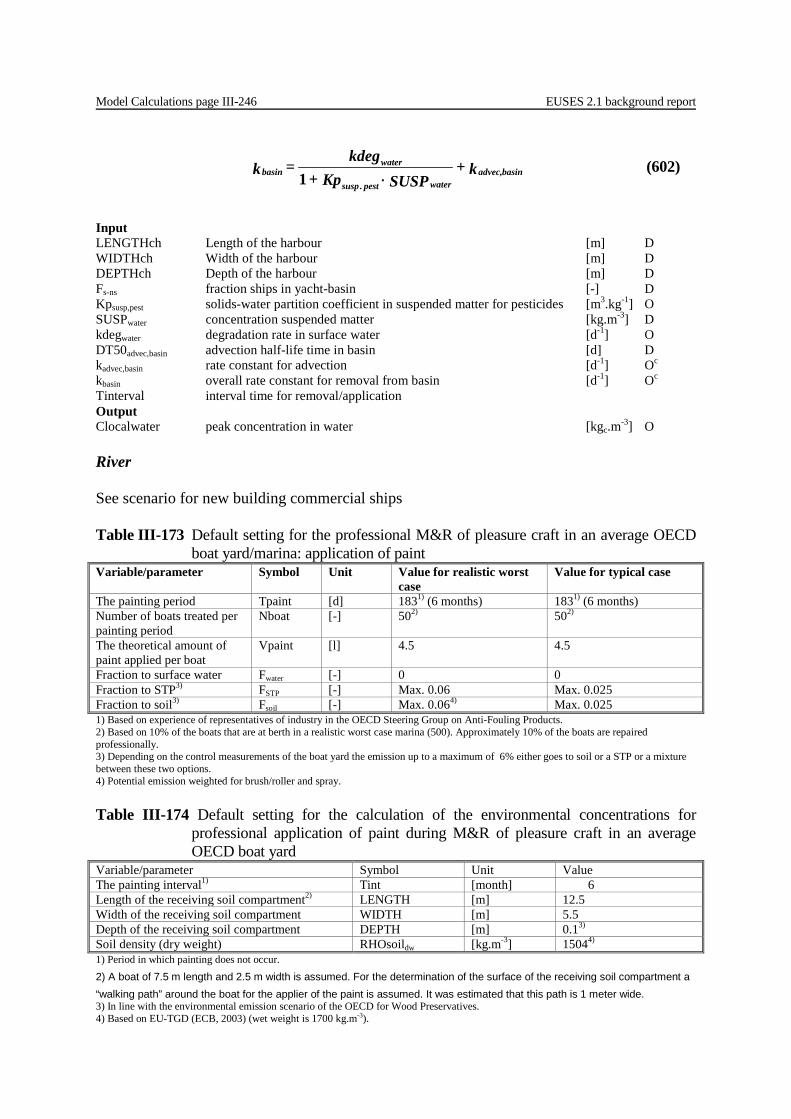
Model Calculations page III-246 EUSES 2.1 background report
k + SUSP Kp +
kdeg= k basinadvec,
waterpestsusp
waterbasin ⋅.1
(602)
Input LENGTHch Length of the harbour [m] D WIDTHch Width of the harbour [m] D DEPTHch Depth of the harbour [m] D Fs-ns fraction ships in yacht-basin [-] D Kpsusp,pest solids-water partition coefficient in suspended matter for pesticides [m3.kg-1] O SUSPwater concentration suspended matter [kg.m-3] D kdegwater degradation rate in surface water [d-1] O DT50advec,basin advection half-life time in basin [d] D kadvec,basin rate constant for advection [d-1] Oc kbasin overall rate constant for removal from basin [d-1] Oc
Tinterval interval time for removal/application Output Clocalwater peak concentration in water [kgc.m-3] O River See scenario for new building commercial ships Table III-173 Default setting for the professional M&R of pleasure craft in an average OECD
boat yard/marina: application of paint Variable/parameter Symbol Unit Value for realistic worst
case Value for typical case
The painting period Tpaint [d] 1831) (6 months) 1831) (6 months) Number of boats treated per painting period
Nboat [-] 502) 502)
The theoretical amount of paint applied per boat
Vpaint [l] 4.5 4.5
Fraction to surface water Fwater [-] 0 0 Fraction to STP3) FSTP [-] Max. 0.06 Max. 0.025 Fraction to soil3) Fsoil [-] Max. 0.064) Max. 0.025 1) Based on experience of representatives of industry in the OECD Steering Group on Anti-Fouling Products. 2) Based on 10% of the boats that are at berth in a realistic worst case marina (500). Approximately 10% of the boats are repaired professionally. 3) Depending on the control measurements of the boat yard the emission up to a maximum of 6% either goes to soil or a STP or a mixture between these two options. 4) Potential emission weighted for brush/roller and spray. Table III-174 Default setting for the calculation of the environmental concentrations for
professional application of paint during M&R of pleasure craft in an average OECD boat yard
Variable/parameter Symbol Unit Value The painting interval1) Tint [month] 6 Length of the receiving soil compartment2) LENGTH [m] 12.5 Width of the receiving soil compartment WIDTH [m] 5.5 Depth of the receiving soil compartment DEPTH [m] 0.13) Soil density (dry weight) RHOsoildw [kg.m-3] 15044) 1) Period in which painting does not occur. 2) A boat of 7.5 m length and 2.5 m width is assumed. For the determination of the surface of the receiving soil compartment a “walking path” around the boat for the applier of the paint is assumed. It was estimated that this path is 1 meter wide. 3) In line with the environmental emission scenario of the OECD for Wood Preservatives. 4) Based on EU-TGD (ECB, 2003) (wet weight is 1700 kg.m-3).

EUSES 2.1 background report Model Calculations page III-247
Table III-175 Default setting for the professional removal of the paint layer in an average OECD boatyard Variable/parameter Symbol Unit Value for realistic worst
case Value for typical case
The removal period Tremoval [d] 1831) (6 months) 1831) (6 months) Number of boats treated per removal period
Nboat [-] 502) 502)
The amount of paint applied per boat
Vpaint [l] 4.5 (as for application) 4.5 (as for application)
Fraction of the paint that is to be removed from the boat hull by HPW3)
Fwashing [-] 0.20 0.20
Fraction of the paint that is to be removed from the boat hull by abrasion3)
Fabrasion [-] 0.10 n/a
Fraction of a.i. remained in exhausted paint removed by washing3)
Fa.i.exh paint [-] 0.05 0.05
Fraction of a.i. remained in old paint removed by abrasion3)
Fa.i.old paint [-] 0.30 n/a
Fraction to surface water4) Fwater [-] Max. 1 Max. 1 Fraction to STP4) FSTP [-] Max. 1 Max. 1 Fraction to soil4) Fsoil [-] Max. 1 Max. 1 1) Based on expert judgement CEPE. 2) Based on 10% of the boats that are at berth in a realistic worst case marina (500). Approximately 10% of the boats are repaired professionally. 3) HP washing will remove only the leached layer. For pleasure boats the leached layer represents typically 20% of the paint film applied (Safinah, 2004) and contains a fraction of 0.05 (expert judgement CEPE) of the original concentration of of a.i. the paint. Abrasion will remove 30% of the old paint film. This 30% consists of the leached layer and an additional layer which contains a fraction of 0.30 (expert judgement CEPE) of the original concentration of of a.i. the paint (see also section Error! Reference source not found.). 4) Depending on the control measurements of the boatyard the emission goes to soil, surface water, or a STP or a mixture between these 3 options. Table III-176 Default setting for the calculation of the local initial environmental
concentrations in soil and surface water for professional application and removal of the paint layer during M&R of pleasure craft in an average OECD boatyard for both realistic worst and typical case
Variable/parameter Unit Symbol Value Soil The removal interval1) [month] Tint 6 Length of the receiving soil compartment2) [m] LENGTH 12.5 Width of the receiving soil compartment [m] WIDTH 5.5 Depth of the receiving soil compartment [m] DEPTH 0.13) Soil density (dry weight) [kg.m-3] RHOsoildw 15044) Surface water Length [m] LENGTHm 141.5 Width [m] WIDTHm 141.5 Depth of harbour [m] DEPTHm 4 Advection time in basin (d-1) DT50advec,basin [d] 50 1) Time period in which removal of paint does not occur. 2) The weighted average boat length of boats > 7.5 m is 10.36 m. A boat of 10.5 m length and 3.5 m width is assumed. For the determination of the surface of the receiving environmental compartment (compacted earth for the realistic worst case scenario) a “walking path” around the boat (width: 1 m) for the applier of the paint is assumed. 3) In line with the environmental emission scenario of the OECD for Wood Preservatives. 4) Based on EU-TGD (ECB, 2003) (wet weight is 1700 kg.m-3).
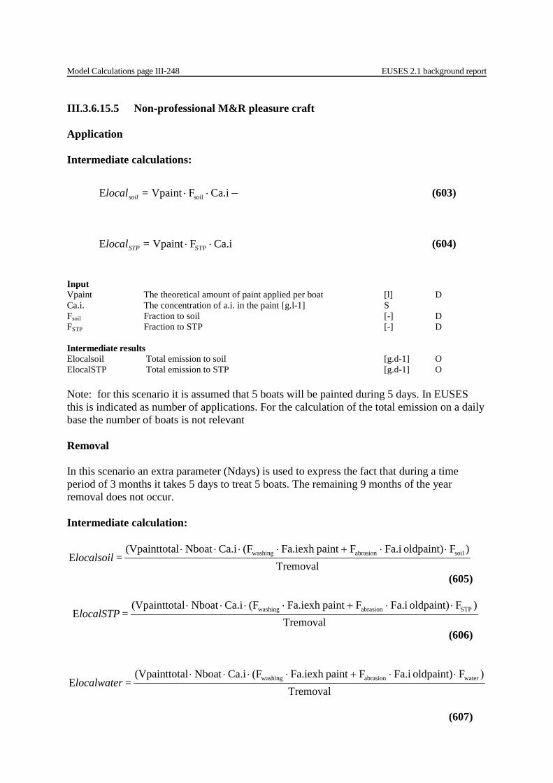
Model Calculations page III-248 EUSES 2.1 background report
III.3.6.15.5 Non-professional M&R pleasure craft Application Intermediate calculations:
= localsoil Ca.iFVpaintE soil ⋅⋅ (603)
= localSTP Ca.iFVpaintE STP ⋅⋅ (604)
Input Vpaint The theoretical amount of paint applied per boat [l] D Ca.i. The concentration of a.i. in the paint [g.l-1] S Fsoil Fraction to soil [-] D FSTP Fraction to STP [-] D Intermediate results Elocalsoil Total emission to soil [g.d-1] O ElocalSTP Total emission to STP [g.d-1] O Note: for this scenario it is assumed that 5 boats will be painted during 5 days. In EUSES this is indicated as number of applications. For the calculation of the total emission on a daily base the number of boats is not relevant Removal In this scenario an extra parameter (Ndays) is used to express the fact that during a time period of 3 months it takes 5 days to treat 5 boats. The remaining 9 months of the year removal does not occur. Intermediate calculation:
= localsoilTremoval
)Foldpaint) Fa.iFpaintFa.iexh (FCa.iNboatal(VpainttotE soilabrasionwashing ⋅⋅+⋅⋅⋅⋅
(605)
= localSTPTremoval
)Foldpaint) Fa.iFpaintFa.iexh (FCa.iNboatal(VpainttotE STPabrasionwashing ⋅⋅+⋅⋅⋅⋅
(606)
= localwaterTremoval
)Foldpaint) Fa.iFpaintFa.iexh (FCa.iNboatal(VpainttotE waterabrasionwashing ⋅⋅+⋅⋅⋅⋅
(607)
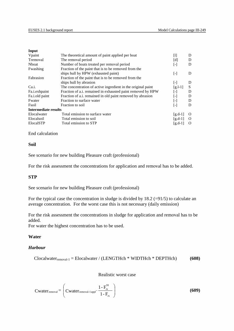
EUSES 2.1 background report Model Calculations page III-249
Input Vpaint The theoretical amount of paint applied per boat [l] D Tremoval The removal period [d] D Nboat Number of boats treated per removal period [-] D Fwashing Fraction of the paint that is to be removed from the
ships hull by HPW (exhausted paint) [-] D Fabrasion Fraction of the paint that is to be removed from the
ships hull by abrasion [-] D Ca.i. The concentration of active ingredient in the original paint [g.l-1] S Fa.i.exhpaint Fraction of a.i. remained in exhausted paint removed by HPW [-] D Fa.i.old paint Fraction of a.i. remained in old paint removed by abrasion [-] D Fwater Fraction to surface water [-] D Fsoil Fraction to soil [-] D Intermediate results Elocalwater Total emission to surface water [g.d-1] O Elocalsoil Total emission to soil [g.d-1] O ElocalSTP Total emission to STP [g.d-1] O End calculation Soil See scenario for new building Pleasure craft (professional) For the risk assessment the concentrations for application and removal has to be added. STP See scenario for new building Pleasure craft (professional) For the typical case the concentration in sludge is divided by 18.2 (=91/5) to calculate an average concentration. For the worst case this is not necessary (daily emission) For the risk assessment the concentrations in sludge for application and removal has to be added. For water the highest concentration has to be used. Water Harbour
Clocalwaterremoval-1 = Elocalwater / (LENGTHch * WIDTHch * DEPTHch) (608)
Realistic worst case
⋅
rs
91rs
appl 1 -removalremoval F- 1 F- 1
Cwater = Cwater (609)
Model Calculations page III-250 EUSES 2.1 background report
intervalsin Tk -rs
bae= F ⋅
sinba,advec
basinadvec, DT50 ln= k2 (610)
k + SUSP Kp +
kdeg= k basinadvec,
waterpestsusp
waterbasin ⋅.1
(611)
Input LENGTHch Length of the harbour [m] D WIDTHch Width of the harbour [m] D DEPTHch Depth of the harbour [m] D Fs-ns fraction ships in yacht-basin [-] D Kpsusp,pest solids-water partition coefficient in suspended matter for pesticides [m3.kg-1] O SUSPwater concentration suspended matter [kg.m-3] D kdegwater degradation rate in surface water [d-1] O DT50advec,basin advection half-life time in basin [d] D kadvec,basin rate constant for advection [d-1] Oc kbasin overall rate constant for removal from basin [d-1] Oc Output Clocalwater peak concentration in water [kgc.m-3] O River See scenario for new building commercial ships Table III-177 Default setting for the non-professional M&R of pleasure craft in an average
OECD marina: application of paint Variable/parameter Unit Symbol Value The painting period [d] Tpaint 911) (3 months) Number of days to paint one boat2) [-] Ndays 1 Number of boats treated per painting period [-] Nboat 53) The theoretical amount of paint applied per boat
[l] Vpaint 2.51)
Fraction to surface water [-] Fwater 0 Fraction to STP4) [-] FSTP Max. 0.025 Fraction to soil4) [-] Fsoil Max. 0.025 1) Expert judgement CEPE. 2) In this scenario an extra parameter (Ndays) is used to express the fact that during a time period of 3 months it takes 5 days to paint 5 boats. The remaining 9 months of the year painting does not occur. 3) 10% of the boats are repaired professionally (Safinah) and that 20% of the boats are not painted at all per year (expert judgement industry). Thus 350 (70%) of the boats that are at berth in a realistic worst case marina (500) are repaired non-professionally each year. During 3 months 350 boats are painted. This does not necessarily happen at the same spot of 9.5 m length and 4.5 m width (boats can be taken home for application or painted in storage area). Therefore it is assumed that only 5 boats are painted on the same spot per painting period (based on Finnish data: In Finland typically 1-5 boats are painted on the same spot). 4) Depending on the control measurements (hard standing area) the emission up to a maximum of 2.5% either goes to soil or a STP or a mixture between these two options. For non-professional application it is most likely that the emission goes to soil.
EUSES 2.1 background report Model Calculations page III-251
Table III-178 Default setting for the calculation of the environmental concentrations for non-
professional application of paint during M&R of pleasure craft in an average OECD marina for both realistic worst case and typical case scenario
Variable/parameter Unit Symbol Value S/D/O/P The painting interval1) [month] Tint 9 D Length of the receiving soil compartment2) [m] LENGTH 9.5 D Width of the receiving soil compartment [m] WIDTH 4.5 D Depth of the receiving soil compartment [m] DEPTH 0.13) D Soil density (dry weight) [kg.m-3] RHOsoildw 15044) 1) Period in which painting does not occur. 2) A boat of 7.5 m length and 2.5 m width is assumed. For the determination of the surface of the receiving soil compartment a “walking path” around the boat for the applier of the paint is assumed. It was estimated that this path is 1 metre wide. 3) In line with the environmental emission scenario of the OECD for Wood Preservatives. 4) Based on EU-TGD (ECB, 2003) (wet weight is 1700 kg.m-3). Table III-179 Default setting for the Non-professional removal of the paint layer in an average
OECD boatyard/marina Variable/parameter Symbol Unit Value for realistic worst
case Value for typical case
The removal period Tremoval [d] 911) (3 months)
911) (3 months)
The number of days for the treatment of one boat5)
Ndays [-] n/a 1
Number of boats treated per removal period
Nboat [-] 3502)
5
The amount of paint applied per boat
Vpaint [l] 2.5
2.5
Fraction of the paint that is to be removed from the boat hull by HPW3)
Fwashing [-] 0.20 n/a
Fraction of the paint that is to be removed from the boat hull by abrasion3)
Fabrasion [-] n/a 0.10
Fraction of a.i. remained in exhausted paint removed by washing3)
Fa.i.exh paint [-] 0.05 n/a
Fraction of a.i. remained in old paint removed by abrasion3)
Fa.i.old paint [-] n/a 0.30
Fraction to surface water4) Fwater [-] Max. 1 n/a Fraction to STP4) FSTP [-] Max. 1
Max. 1
Fraction to soil4) Fsoil [-] Max. 1 Max. 1 1) Based on expert judgement of CEPE. 2) Based on the fact that 10% of the boats are repaired professionally (Safinah 2004) and that 20% of the boats are not painted at all per year (expert judgement industry). Thus 70% of the boats that are at berth in a realistic worst case marina (500) are repaired non-professionally each year. 3) HP washing will remove only the leached layer. For pleasure boats the leached layer represents typically 20% of the paint film applied (Safinah, 2004) and contains a fraction of 0.05 (expert judgement CEPE) of the original concentration of of a.i. the paint. Abrasion will remove 30% of the old paint film. This 30% consists of the leached layer and an additional layer which contains a fraction of 0.30 (expert judgement CEPE) of the original concentration of of a.i. the paint. 4) Depending on the control measurements of the boatyard the emission goes to soil, surface water or a STP or a mixture between these 3 options. 5) In this scenario an extra parameter (Ndays) is used to express the fact that during a time period of 3 months it takes 5 days to treat 5 boats. The remaining 9 months of the year removal does not occur.
Model Calculations page III-252 EUSES 2.1 background report
Table III-180 Default setting for calculation of the environmental concentrations in soil and surface water for non-professional removal of the paint layer in an average OECD boatyard/marina (see M&R) for both realistic worst and typical case
Variable/parameter Symbol Unit Value Soil The removal interval1) Tint [month-1] 9 The removal frequency Tfreq [-] 5 Length of the receiving soil compartment2) LENGTH [m] 9.5 Width of the receiving soil compartment WIDTH [m] 4.5 Depth of the receiving soil compartment DEPTH [m] 0.13) Soil density (dry weight) RHOsoildw [kg.m-3] 15044) Surface water Length LENGTHm [m] 141.5 Width WIDTHm [m] 141.5 Depth of harbour DEPTHm [m] 4 Advection time in basin (d-1) DT50advec,basin [d] 50 1) Time period in which removal of paint does not occur. 2) A boat of 7.5 m length and 2.5 m width is assumed. For the determination of the surface of the receiving soil compartment a “walking path” around the boat for the applier of the paint is assumed. It was estimated that this path is 1 metre wide. 3) In line with the environmental emission scenario of the OECD for Wood Preservatives. 4) Based on EU-TGD (ECB, 2003) (wet weight is 1700 kg.m-3).
EUSES 2.1 background report Model Calculations page III-253
III.3.6.16 Embalming and taxidermist fluids The scenarios and models and calculation formulations used in this version of EUSES 2.1.1 for insecticides have been taken from the following document:
− European Union System for the Evaluation of Substances, EUSES 2.0 (EC, 2004)
Taxidermy includes the preservation of animals and concerns as well as large mammals, fishes, birds and reptiles. Embalming consist of three different procedures which involve the use of biocides: surface disinfection (soaps, solutions), arterial injection of fluids and injection of cavity fluids into the torso to substitute body fluids. III.3.6.16.1 Biocides used in taxidermy Model for calculating release to water for compounds used in taxidermist fluids. Ffix) -(1Qsubst Qskin= erElocal_wat i ⋅⋅ (612)
iwater erElocal_wat= Elocal ∑ (613)
Input Qskin quantity of treated drained skin per day [kg.d-1] D - type of agent per treatment step [-] P Qsubst quantity of active substance applied per kg of drained skin [kg.kg-1] O Ffix fixation fraction [-] S/D Elocal_wateri local emission of active substance to waste water for treatment [kg.d-1] O step i Output Elocalwater local emission of active substance to waste water for all [kgc.d-1] O treatment steps Table III-181 Default settings of the model for calculating the release of biocides used in
taxidermy. Parameter Symbol Unit Value
Quantity of treated drained skin per day Qskin [kg.d-1] 4
Quantity of active substance applied per kg of drained
skin
Pickling
- formaldehyde
- tanning agent
Soaking
- bactericide
Preservation
- insecticide
Qsubst [kg.kg-1] 0.02
0.005
0.02
0.002
0.02
Fixation fraction Ffix [-] 0.95
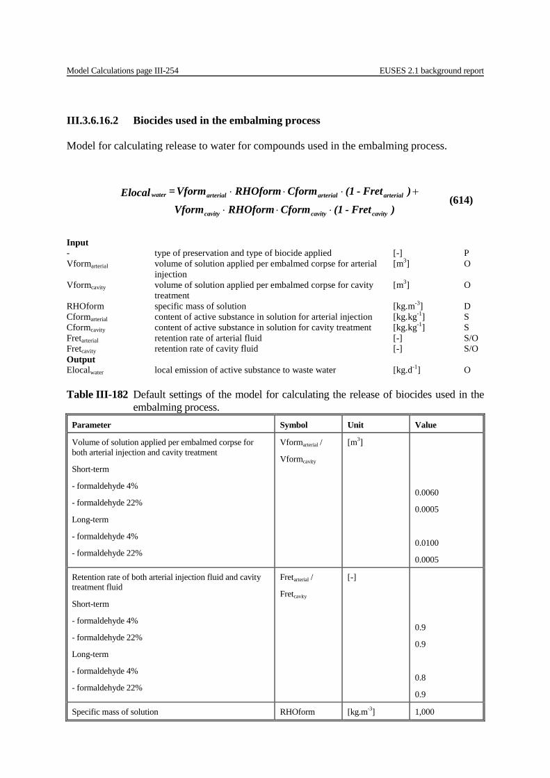
Model Calculations page III-254 EUSES 2.1 background report
III.3.6.16.2 Biocides used in the embalming process Model for calculating release to water for compounds used in the embalming process.
)Fret -(1CformRHOform Vform
)Fret -(1CformRHOform Vform= Elocal
cavitycavitycavity
arterialarterialarterialwater
⋅⋅⋅
+⋅⋅⋅ (614)
Input - type of preservation and type of biocide applied [-] P Vformarterial volume of solution applied per embalmed corpse for arterial [m3] O injection Vformcavity volume of solution applied per embalmed corpse for cavity [m3] O treatment RHOform specific mass of solution [kg.m-3] D Cformarterial content of active substance in solution for arterial injection [kg.kg-1] S Cformcavity content of active substance in solution for cavity treatment [kg.kg-1] S Fretarterial retention rate of arterial fluid [-] S/O Fretcavity retention rate of cavity fluid [-] S/O Output Elocalwater local emission of active substance to waste water [kg.d-1] O Table III-182 Default settings of the model for calculating the release of biocides used in the
embalming process. Parameter Symbol Unit Value
Volume of solution applied per embalmed corpse for both arterial injection and cavity treatment
Short-term
- formaldehyde 4%
- formaldehyde 22%
Long-term
- formaldehyde 4%
- formaldehyde 22%
Vformarterial /
Vformcavity
[m3]
0.0060
0.0005
0.0100
0.0005
Retention rate of both arterial injection fluid and cavity treatment fluid
Short-term
- formaldehyde 4%
- formaldehyde 22%
Long-term
- formaldehyde 4%
- formaldehyde 22%
Fretarterial /
Fretcavity
[-]
0.9
0.9
0.8
0.9
Specific mass of solution RHOform [kg.m-3] 1,000
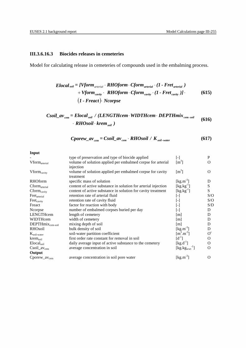
EUSES 2.1 background report Model Calculations page III-255
III.3.6.16.3 Biocides releases in cemeteries Model for calculating release in cemeteries of compounds used in the embalming process.
( ) NcorpseFreact-1
)]Fret -(1CformRHOform Vform)Fret -(1CformRHOform [Vform= Elocal
cavitycavitycavity
arterialarterialsoil
⋅
⋅⋅⋅⋅+
⋅⋅⋅arterial
(615)
)kremRHOsoil
DEPTHmixWIDTHcem(LENGTHcem / Elocal= Csoil_av
soil
soil-cemsoilcem
⋅⋅
⋅⋅ (616)
water-soilcemcem K / RHOsoil Csoil_av= Cporew_av ⋅ (617)
Input - type of preservation and type of biocide applied [-] P Vformarterial volume of solution applied per embalmed corpse for arterial [m3] O injection Vformcavity volume of solution applied per embalmed corpse for cavity [m3] O treatment RHOform specific mass of solution [kg.m-3] D Cformarterial content of active substance in solution for arterial injection [kg.kg-1] S Cformcavity content of active substance in solution for cavity treatment [kg.kg-1] S Fretarterial retention rate of arterial fluid [-] S/O Fretcavity retention rate of cavity fluid [-] S/O Freact factor for reaction with body [-] S/D Ncorpse number of embalmed corpses buried per day [-] D LENGTHcem length of cemetery [m] D WIDTHcem width of cemetery [m] D DEPTHmixcem-soil mixing depth of soil [m] D RHOsoil bulk density of soil [kg.m-3] D Ksoil-water soil-water partition coefficient [m3.m-3] Oc kremsoil first order rate constant for removal in soil [d-1] O Elocalsoil daily average input of active substance to the cemetery [kg.d-1] O Csoil_avcem average concentration in soil [kg.kgwwt
-1] O Output Cporew_avcem average concentration in soil pore water [kg.m-3] O
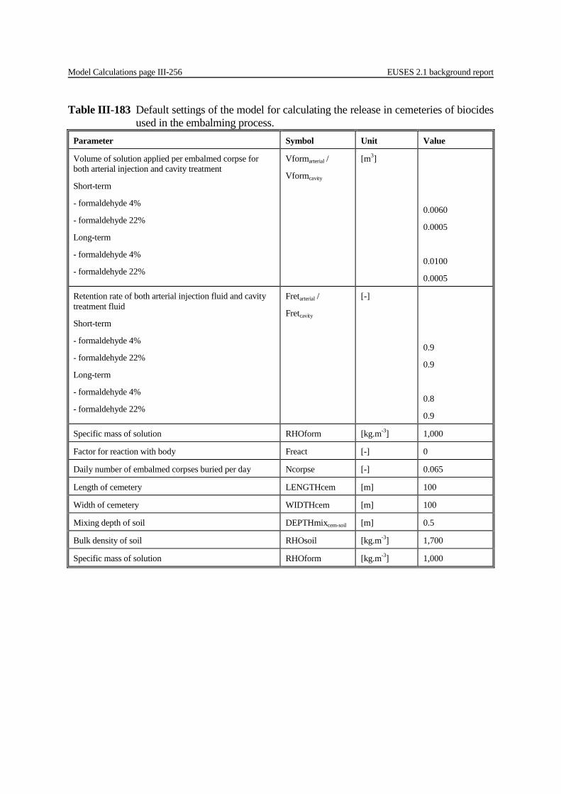
Model Calculations page III-256 EUSES 2.1 background report
Table III-183 Default settings of the model for calculating the release in cemeteries of biocides used in the embalming process.
Parameter Symbol Unit Value
Volume of solution applied per embalmed corpse for both arterial injection and cavity treatment
Short-term
- formaldehyde 4%
- formaldehyde 22%
Long-term
- formaldehyde 4%
- formaldehyde 22%
Vformarterial /
Vformcavity
[m3]
0.0060
0.0005
0.0100
0.0005
Retention rate of both arterial injection fluid and cavity treatment fluid
Short-term
- formaldehyde 4%
- formaldehyde 22%
Long-term
- formaldehyde 4%
- formaldehyde 22%
Fretarterial /
Fretcavity
[-]
0.9
0.9
0.8
0.9
Specific mass of solution RHOform [kg.m-3] 1,000
Factor for reaction with body Freact [-] 0
Daily number of embalmed corpses buried per day Ncorpse [-] 0.065
Length of cemetery LENGTHcem [m] 100
Width of cemetery WIDTHcem [m] 100
Mixing depth of soil DEPTHmixcem-soil [m] 0.5
Bulk density of soil RHOsoil [kg.m-3] 1,700
Specific mass of solution RHOform [kg.m-3] 1,000
EUSES 2.1 background report Model Calculations page III-257
References RIVM, VROM, VWS (2002). Uniform System for the Evaluation of Substances 4.0 (USES 4.0). National Institute of Public Health and the Environment (RIVM), Ministry of Housing, Spatial Planning and the Environment (VROM), Ministry of Health, Welfare and Sport (VWS), The Netherlands. RIVM report no. 601450012. Zandt, P. van der and Balk, F. (2004). Development of Environmental Emission Scenarios for Active Substances used in Biocidal Products. European Commission DG ENV. Service contract B4-3040/2001/326154/MAR/C3. Poel, P van der and Bakker, J. (2002). Emission Scenario Document for Biocides. Emission Scenarios for all 23 product types of the Biocidal Product Directive (EU Directive 98/8/EC). National Institute of Public Health and the Environment (RIVM), Biltoven, the Netherlands. RIVM report no. 601450009. EC (2004). European Union System for the Evaluation of Substances 2.0 (EUSES 2.0). Prepared for the European Chemicals Bureau by the National Institute of Public Health and the Environment (RIVM), Bilthoven, the Netherlands. Avialable via the European Chemicals Bureau, http://ecb.jrc.it. EC (2003). Technical Guidance Document on Risk Assessment (TGD) in support of Commission Directive 93/67/EEC, Commission Regulation (EC) No 1488/94 on Risk Assessment for Existing substances, Directive 98/8/EC of the European Parliament and of the Council concerning the placing of biocidal products on the market.
Model Calculations page III-258 EUSES 2.1 background report
III.4 ENVIRONMENTAL DISTRIBUTION In the environmental distribution module, five sub-modules are specified: • Estimation of partition coefficients. • Estimation of environmental degradation rates. • Fate in sewage treatment. • Regional environmental distribution. • Local environmental distribution. Environmental distribution is estimated on three spatial scales: local, regional and continental. The environmental characteristics of these scales are (by default) the same. III.4.1 Partition coefficients In this section, the characteristics of the environmental compartments are defined. From this definition, the bulk densities of soil, sediment and suspended matter are calculated. The following partitioning processes are quantified in this section: • Adsorption to aerosol particles. • Air-water partitioning. • Adsorption/desorption to solids in soil, sediment, suspended matter and sewage sludge. The output parameters for bulk densities of compartments and 'dimensionless partition coefficients' are closed for the user. This is done for the sake of internal consistency. For example bulk density of soil is defined by the fractions and densities of the separate phases (solids, water, air). The bulk density should not be changed without changing the fractions or densities of the phases.

EUSES 2.1 background report Model Calculations page III-259
Input VP vapour pressure [Pa] MOLW molecular weight [kgc.mol-1] SOL solubility [kgc.m-3] Kow octanol-water partition coefficient [-] TEMPmelt melting point (only for solids for estimating Fassaer) [K] Intermediate results VPL sub-cooled liquid vapour pressure [Pa] Koc organic carbon-water partition coefficient [m3.kg-1] Output 1 RHOsoil wet bulk density of soil [kgwwt.m-3] c RHOsed wet bulk density of sediment [kgwwt.m-3] c RHOsusp wet bulk density of suspended matter [kgwwt.m-3] c CONVsoil conversion factor for soil concentrations: wwt to dwt [kgwwt.kgdwt
-1] c CONVsed conversion factor for sediment concentrations: wwt to dwt [kgwwt.kgdwt
-1] c Fassaer fraction of chemical associated with aerosol particles [-] HENRY Henry's law constant [Pa.m3.mol-1] Kpsusp solids-water partition coefficient in suspended matter [m3.kg-1] Kpsed solids-water partition coefficient in sediment [m3.kg-1] Kpsoil solids-water partition coefficient in soil [m3.kg-1] KpRS solids-water partition coeff. in raw sewage sludge [m3.kg-1] KpPS solids-water partition coeff. in settled sewage sludge [m3.kg-1] KpA solids-water partition coeff. in activated sewage sludge [m3.kg-1] KpSLS solids-water partition coeff. in effluent sewage sludge [m3.kg-1] Output 2 (internal parameters) Kair-water air-water partition coefficient [m3.m-3] c Ksoil-water soil-water partition coefficient [m3.m-3] c Ksusp-water suspended matter-water partition coefficient [m3.m-3] c Ksed-water sediment-water partition coefficient [m3.m-3] c
Model Calculations page III-260 EUSES 2.1 background report
III.4.1.1 Bulk densities of compartments Each of the compartments soil, sediment, and suspended matter is described as consisting of three phases: air (relevant in soil only), solids and water. The bulk density of each compartment is thus defined by the fraction and bulk density of each phase. Both the fractions of solids and water, and the total bulk density are used in subsequent calculations. This implies that the bulk
Table III-184 Default environmental characteristics for local, regional and continental scales Parameter Symbol Unit Value
General
Density of solid phase RHOsolid [kgsolid.msolid-3] 2500
Density of water phase RHOwater [kgwater.mwater-3] 1000
Density of air RHOair [kgair.mair-3] 1.3
Environmental temperature Freshwater environment (12 °C)
Marine environment (12 °C)
TEMP [K] 285 285 c
Constant of Junge equation CONjunge [Pa.m] a
Specific surface area of aerosol particles SURFaer [m2.m-3] a
Gas constant R [Pa.m3.mol-1.K-1] 8.314 b
Suspended matter
Volume fraction of solids in susp. matter Fsolidsusp [msolid3.msusp
-3] 0.1
Volume fraction of water in susp. matter Fwatersusp [mwater3.msusp
-3] 0.9
Weight fraction of organic carbon in susp. solids Focsusp [kgoc.kgsolid-1] 0.1
Sediment
Volume fraction of solids in sediment Fsolidsed [msolid3.msed
-3] 0.2
Volume fraction of water in sediment Fwatersed [mwater3.msed
-3] 0.8
Weight fraction of organic carbon sediment solids Focsed [kgoc.kgsolid-1] 0.05
Soil
Volume fraction of solids in soil Fsolidsoil [msolid3.msoil
-3] 0.6
Volume fraction of water in soil Fwatersoil [mwater3.msoil
-3] 0.2
Volume fraction of air in soil Fairsoil [mair3.msoil
-3] 0.2
Weight fraction of organic carbon in soil solids Focsoil [kgoc.kgsolid-1] 0.02
a By default, the product of CONjunge and SURFaer is set to 10-4 Pa (Van de Meent, 1993); Den Hollander and Van de Meent (2004) uses 2.58.10-5 Pa. b This default cannot be changed by the user. c Although the TGD (2003) proposed a temperature of 9 °C, due to the small differences it was decided to keep the temperature the same for all compartments on the moderate global scale the same.
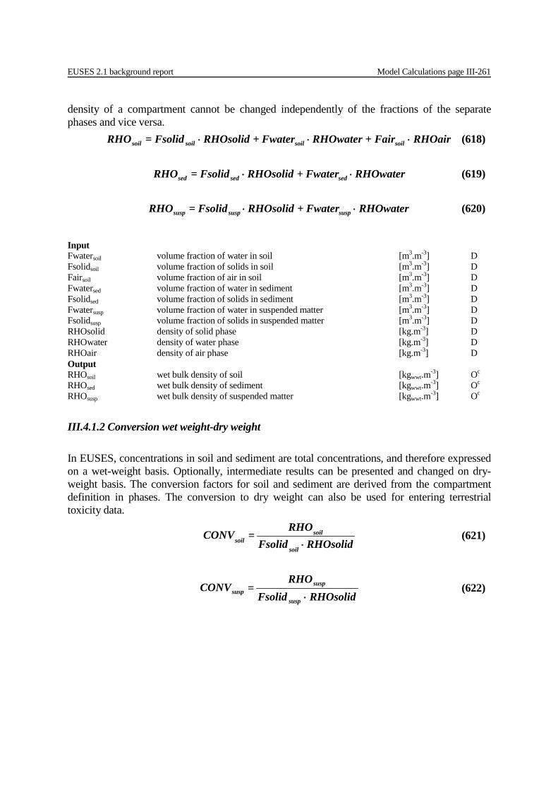
EUSES 2.1 background report Model Calculations page III-261
density of a compartment cannot be changed independently of the fractions of the separate phases and vice versa.
Input Fwatersoil volume fraction of water in soil [m3.m-3] D Fsolidsoil volume fraction of solids in soil [m3.m-3] D Fairsoil volume fraction of air in soil [m3.m-3] D Fwatersed volume fraction of water in sediment [m3.m-3] D Fsolidsed volume fraction of solids in sediment [m3.m-3] D Fwatersusp volume fraction of water in suspended matter [m3.m-3] D Fsolidsusp volume fraction of solids in suspended matter [m3.m-3] D RHOsolid density of solid phase [kg.m-3] D RHOwater density of water phase [kg.m-3] D RHOair density of air phase [kg.m-3] D Output RHOsoil wet bulk density of soil [kgwwt.m-3] Oc RHOsed wet bulk density of sediment [kgwwt.m-3] Oc RHOsusp wet bulk density of suspended matter [kgwwt.m-3] Oc
III.4.1.2 Conversion wet weight-dry weight In EUSES, concentrations in soil and sediment are total concentrations, and therefore expressed on a wet-weight basis. Optionally, intermediate results can be presented and changed on dry-weight basis. The conversion factors for soil and sediment are derived from the compartment definition in phases. The conversion to dry weight can also be used for entering terrestrial toxicity data.
RHOair Fair+ RHOwaterFwater+ RHOsolid Fsolid= RHO soilsoilsoilsoil ⋅⋅⋅ (618)
RHOwaterFwater+ RHOsolid = FsolidRHO sedsedsed ⋅⋅ (619)
RHOwater Fwater+ RHOsolid= FsolidRHO suspsuspsusp ⋅⋅ (620)
RHOsolidFsolid
RHO= CONV
soil
soilsoil ⋅
(621)
RHOsolidFsolid
RHO= CONV
susp
suspsusp ⋅
(622)
Model Calculations page III-262 EUSES 2.1 background report
Input RHOsoil wet bulk density of soil [kgwwt.m-3] Oc Fsolidsoil volume fraction of solids in soil [m3.m-3] D RHOsusp wet bulk density of suspended matter [kgwwt.m-3] Oc Fsolidsusp volume fraction of solids in suspended matter [m3.m-3] D RHOsolid density of solid phase [kg.m-3] D Output CONVsoil conversion factor for soil concentrations: wwt to dwt [kgwwt.kgdwt
-1] Oc CONVsusp conversion factor for suspended matter conc.: wwt to dwt [kgwwt.kgdwt
-1] Oc
III.4.1.3 Adsorption to aerosol particles The fraction of the chemical associated with aerosol particles can be estimated on the basis of the chemical's vapour pressure, according to Junge (1977). In this equation, the sub-cooled liquid vapour pressure should be used. For solids, a correction is applied according to Mackay (1991).
If TEMPmelt <= TEMP (substance is liquid):
If TEMPmelt > TEMP (substance is solid):
Input CONjunge constant of Junge equation [Pa.m] D SURFaer surface area of aerosol particles [m2.m-3] D VP vapour pressure [Pa] S TEMP environmental temperature [K] D TEMPmelt melting point of substance [K] S Output VPL sub-cooled liquid vapour pressure [Pa] O Fassaer fraction of chemical associated with aerosol particles [-] O
III.4.1.4 Air-water partitioning The transfer of substances from the aqueous phase to the gas phase (e.g. stripping in the aeration tank of an STP, volatilisation from surface water) is estimated by means of its Henry's Law constant. If the value is not available in the input dataset, the required Henry's Law constant and Kair-water (also known as the 'dimensionless' Henry's Law constant) can be estimated from the ratio of the vapour pressure to the water solubility:
SURF CONjunge + VP
SURF CONjunge = FassaerL
aeraer ⋅
⋅ (623)
VPVPL = (624)
e
VP= VP
TEMPTEMPmelt -
L
179.6
(625)
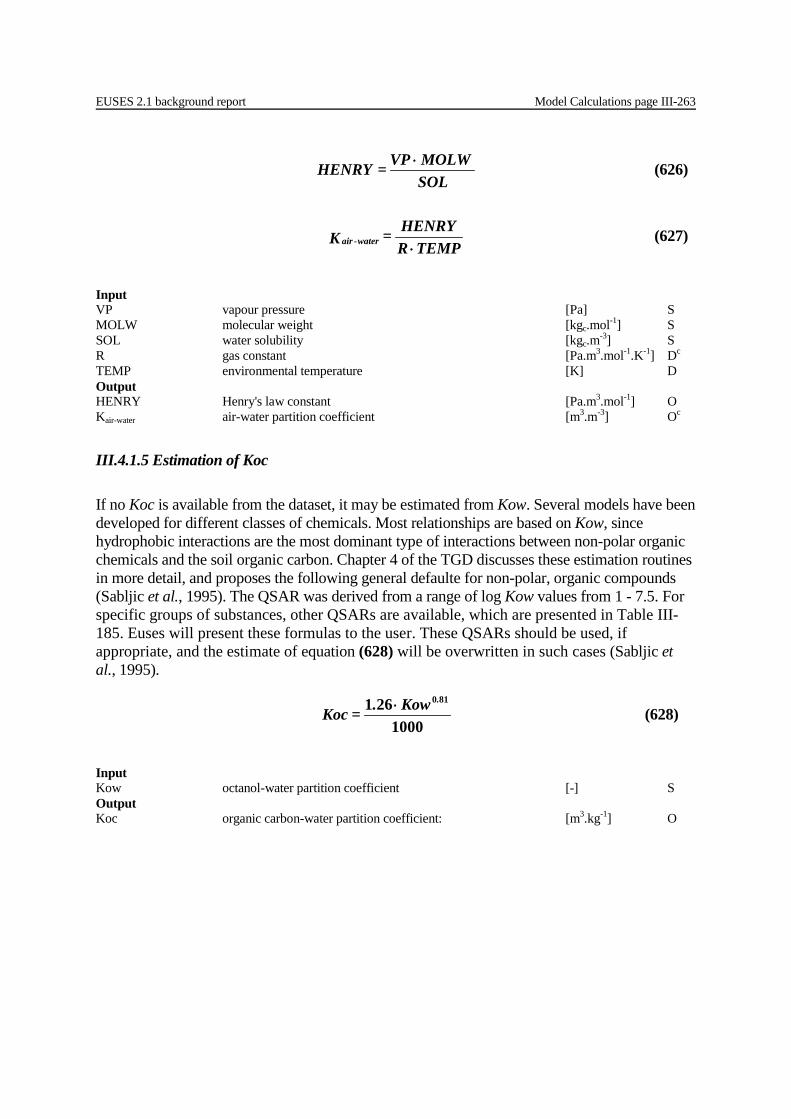
EUSES 2.1 background report Model Calculations page III-263
Input VP vapour pressure [Pa] S MOLW molecular weight [kgc.mol-1] S SOL water solubility [kgc.m-3] S R gas constant [Pa.m3.mol-1.K-1] Dc TEMP environmental temperature [K] D Output HENRY Henry's law constant [Pa.m3.mol-1] O Kair-water air-water partition coefficient [m3.m-3] Oc
III.4.1.5 Estimation of Koc If no Koc is available from the dataset, it may be estimated from Kow. Several models have been developed for different classes of chemicals. Most relationships are based on Kow, since hydrophobic interactions are the most dominant type of interactions between non-polar organic chemicals and the soil organic carbon. Chapter 4 of the TGD discusses these estimation routines in more detail, and proposes the following general defaulte for non-polar, organic compounds (Sabljic et al., 1995). The QSAR was derived from a range of log Kow values from 1 - 7.5. For specific groups of substances, other QSARs are available, which are presented in Table III-185. Euses will present these formulas to the user. These QSARs should be used, if appropriate, and the estimate of equation (628) will be overwritten in such cases (Sabljic et al., 1995).
Input Kow octanol-water partition coefficient [-] S Output Koc organic carbon-water partition coefficient: [m3.kg-1] O
SOLMOLW VP= HENRY ⋅ (626)
TEMP R
HENRY= K water-air ⋅ (627)
1000
261 810.Kow.= Koc ⋅ (628)
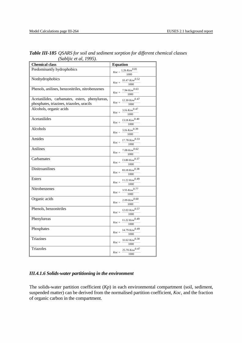
Model Calculations page III-264 EUSES 2.1 background report
Table III-185 QSARS for soil and sediment sorption for different chemical classes
(Sabljic et al, 1995). Chemical class Equation Predominantly hydrophobics
1000
810261 .Kow.Koc = ⋅
Nonhydrophobics 1000
5204710 .Kow.Koc =
⋅
Phenols, anilines, benzonitriles, nitrobenzenes 1000
630947 .Kow.Koc =
⋅
Acetanilides, carbamates, esters, phenylureas, phosphates, triazines, triazoles, uracils 1000
4703012 .Kow.Koc =
⋅
Alcohols, organic acids 1000
470163 .Kow.Koc =
⋅
Acetanilides 1000
4001813 .Kow.Koc =
⋅
Alcohols 1000
390163 .Kow.Koc =
⋅
Amides 1000
3307817 .Kow.Koc =
⋅
Anilines 1000
620087 .Kow.Koc =
⋅
Carbamates 1000
3708013 .Kow.Koc =
⋅
Dinitroanilines 1000
3801883 .Kow.Koc =
⋅
Esters 1000
4902211 .Kow.Koc =
⋅
Nitrobenzenes 1000
770553 .Kow.Koc =
⋅
Organic acids 1000
600092 .Kow.Koc =
⋅
Phenols, benzonitriles 1000
5700212 .Kow.Koc =
⋅
Phenylureas 1000
4902211 .Kow.Koc =
⋅
Phosphates 1000
4907914 .Kow.Koc =
⋅
Triazines 1000
3006231 .Kow.Koc =
⋅
Triazoles 1000
4707025 .Kow.Koc =
⋅
III.4.1.6 Solids-water partitioning in the environment The solids-water partition coefficient (Kp) in each environmental compartment (soil, sediment, suspended matter) can be derived from the normalised partition coefficient, Koc, and the fraction of organic carbon in the compartment.

EUSES 2.1 background report Model Calculations page III-265
Input Focsoil weight fraction of organic carbon in soil [kg.kg-1] D Focsed weight fraction of organic carbon in sediment [kg.kg-1] D Focsusp weight fraction of organic carbon in suspended matter [kg.kg-1] D Koc organic carbon-water partition coefficient [m3.kg-1] O Output Kpsusp solids-water partition coefficient in suspended matter [m3.kg-1] O Kpsed solids-water partition coefficient in sediment [m3.kg-1] O Kpsoil solids-water partition coefficient in soil [m3.kg-1] O
Koc = Foc Kp soilsoil ⋅ (629)
Koc = Foc Kp sedsed ⋅ (630)
Koc = Foc Kp suspsusp ⋅ (631)
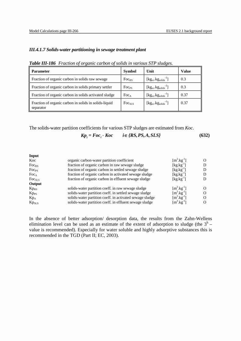
Model Calculations page III-266 EUSES 2.1 background report
III.4.1.7 Solids-water partitioning in sewage treatment plant
The solids-water partition coefficients for various STP sludges are estimated from Koc.
Input Koc organic carbon-water partition coefficient [m3.kg-1] O FocRS fraction of organic carbon in raw sewage sludge [kg.kg-1] D FocPS fraction of organic carbon in settled sewage sludge [kg.kg-1] D FocA fraction of organic carbon in activated sewage sludge [kg.kg-1] D FocSLS fraction of organic carbon in effluent sewage sludge [kg.kg-1] D Output KpRS solids-water partition coeff. in raw sewage sludge [m3.kg-1] O KpPS solids-water partition coeff. in settled sewage sludge [m3.kg-1] O KpA solids-water partition coeff. in activated sewage sludge [m3.kg-1] O KpSLS solids-water partition coeff. in effluent sewage sludge [m3.kg-1] O In the absence of better adsorption/ desorption data, the results from the Zahn-Wellens elimination level can be used as an estimate of the extent of adsorption to sludge (the 3h –value is recommended). Especially for water soluble and highly adsorptive substances this is recommended in the TGD (Part II; EC, 2003).
Table III-186 Fraction of organic carbon of solids in various STP sludges. Parameter Symbol Unit Value
Fraction of organic carbon in solids raw sewage FocRS [kgoc.kgsolids-1] 0.3
Fraction of organic carbon in solids primary settler FocPS [kgoc.kgsolids-1] 0.3
Fraction of organic carbon in solids activated sludge FocA [kgoc.kgsolids-1] 0.37
Fraction of organic carbon in solids in solids-liquid separator
FocSLS [kgoc.kgsolids-1] 0.37
SLS}A,PS,{RS, i Koc = Foc Kp ii ∈⋅ (632)

EUSES 2.1 background report Model Calculations page III-267
III.4.1.8 Total compartment-water partitioning Kp describes the partitioning between solids and water in a compartment. The 'dimensionless' form of Kp, or the total compartment-water partition coefficient, is derived from the definition of the compartments in three phases.
Input Fwatersoil fraction of water in soil [m3.m-3] D Fsolidsoil fraction of solids in soil [m3.m-3] D Fairsoil fraction of air in soil [m3.m-3] D Fwatersed fraction of water in sediment [m3.m-3] D Fsolidsed fraction of solids in sediment [m3.m-3] D Fwatersusp fraction of water in suspended matter [m3.m-3] D Fsolidsusp fraction of solids in suspended matter [m3.m-3] D RHOsolid density of solid phase [kg.m-3] D Kpsoil solids-water partition coefficient in soil [m3.kg-1] O Kpsed solids-water partition coefficient in sediment [m3.kg-1] O Kpsusp solids-water partition coefficient in suspended matter [m3.kg-1] O Kair-water air-water partition coefficient [m3.m-3] Oc Output Ksoil-water total soil-water partition coefficient [m3.m-3] Oc Ksusp-water total suspended matter-water partition coefficient [m3.m-3] Oc Ksed-water total sediment-water partition coefficient [m3.m-3] Oc
RHOsolid Kp Fsolid + Fwater + K Fair= K soilsoilsoilwater-airsoilwater-soil ⋅⋅⋅ (633)
RHOsolid Kp Fsolid + Fwater= K suspsuspsuspwater-susp ⋅⋅ (634)
RHOsolid Kp Fsolid + Fwater= K sedsedsedwater-sed ⋅⋅ (635)

Model Calculations page III-268 EUSES 2.1 background report
III.4.2 Degradation and transformation rates Since measured data on degradation processes for different compartments are not usually available, they must be extrapolated from standardised laboratory tests. In this section, degradation rate constants are derived for abiotic degradation in surface water (hydrolysis and photolysis) and biotic degradation (in soil, sediment, water and sewage treatment). Abiotic degradation in marine environments should be assessed in a similar manner to abiotic degradation in freshwater environments except that the different physico-chemical conditions in marine environments should be taken into account. Abiotic degradation is not estimated for the compartments soil, sediment and STP. If rate constants are known, their default setting of zero (see table below) may be changed. Input characterisation of biodegradability (ready/inherent/non-biodegradable/specific criteria) TEMPtest temperature of the measured data in standard/simulation test [K] DT50hydrwater_temp test half-life for hydrolysis in water at the temperature of the data set [d] DT50photowater half-life for photolysis in water [d] kOH specific degradation rate constant with OH-radicals [m3.molec-1.d-1] DT50biowater_temp test half-life for biodegradation in water at temperature of the data set [d] DT50biosoil_temp test half-life for biodegradation in soil at temperature of data set [d] DT50bio-aersed_temp test half-life for biodeg. in aerobic sediment at temperature of data set [d] Intermediate results DT50hydrwater_temp env half-life for hydrolysis in water at the environmental temperature [d] DT50biostp half-life for biodegradation in STP [d] DT50biowater half-life for biodegradation in bulk surface water [d] DT50biowater_temp env half-life for biodegradation in water at the environmental temp. [d] DT50biosoil half-life for biodegradation in bulk soil [d] DT50biosoil_temp env half-life for biodegradation in soil at the environmental temp. [d] DT50bio-aersed half-life for biodegradation in aerobic sediment [d] DT50bio-aersed_temp env half-life for biodeg. in aerobic sediment at environmental temp. [d] Output kdegair total rate constant for degradation in air [d-1] kdegstp total rate constant for degradation in STP [d-1] kdegwater total rate constant for degradation in bulk surface water [d-1] kdegsoil total rate constant for biodegradation in bulk soil [d-1] kdegsed total rate constant for biodegradation in bulk sediment [d-1] Table III-187 Defaults for calculating degradation rates.
Parameter Symbol Unit Value
Concentration of OH-radicals in atmosphere OHCONCair [molecules.m-3] 5.1011
Fraction of sediment compartment that is aerated Faersed [m3.m-3] 0.10
Rate constant for abiotic degradation in STP kabiostp [d-1] 0
Rate constant for abiotic degradation in soil kabiosoil [d-1] 0
Rate constant for abiotic degradation in sediment kabiosed [d-1] 0
Rate constant for anaerobic biodegr. in sediment kbio-anaersed [d-1] 0
Environmental temperature Freshwater environment (12 °C) Marine environment (12 °C)
TEMP [K] 285 285 a
a Although the TGD (2003) proposed a temperature of 9 °C, due to the small differences it was decided to keep the temperature the same for all compartments on the moderate global scale the same.
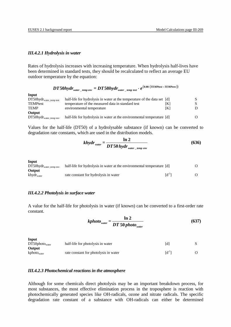
EUSES 2.1 background report Model Calculations page III-269
III.4.2.1 Hydrolysis in water Rates of hydrolysis increases with increasing temperature. When hydrolysis half-lives have been determined in standard tests, they should be recalculated to reflect an average EU outdoor temperature by the equation:
( )( )TEMPenvTEMPtesttesttempwaterenvtempwater e hydrDT= hydrDT −⋅⋅ 08.0
__ 5050 Input DT50hydrwater_temp test half-life for hydrolysis in water at the temperature of the data set [d] S TEMPtest temperature of the measured data in standard test [K] S TEMP environmental temperature [K] D Output DT50hydrwater_temp env half-life for hydrolysis in water at the environmental temperature [d] O Values for the half-life (DT50) of a hydrolysable substance (if known) can be converted to degradation rate constants, which are used in the distribution models.
Input DT50hydrwater_temp env half-life for hydrolysis in water at the environmental temperature [d] O Output khydrwater rate constant for hydrolysis in water [d-1] O
III.4.2.2 Photolysis in surface water A value for the half-life for photolysis in water (if known) can be converted to a first-order rate constant.
Input DT50photowater half-life for photolysis in water [d] S Output kphotowater rate constant for photolysis in water [d-1] O
III.4.2.3 Photochemical reactions in the atmosphere Although for some chemicals direct photolysis may be an important breakdown process, for most substances, the most effective elimination process in the troposphere is reaction with photochemically generated species like OH-radicals, ozone and nitrate radicals. The specific degradation rate constant of a substance with OH-radicals can either be determined
hydrDT
= khydrenvtempwater
water_50
2ln (636)
photoDT
= kphotowater
water 502ln (637)
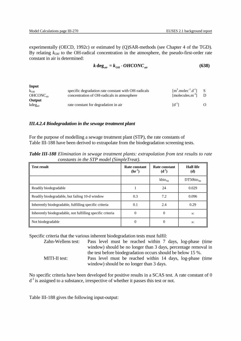
Model Calculations page III-270 EUSES 2.1 background report
experimentally (OECD, 1992c) or estimated by (Q)SAR-methods (see Chapter 4 of the TGD). By relating kOH to the OH-radical concentration in the atmosphere, the pseudo-first-order rate constant in air is determined:
Input kOH specific degradation rate constant with OH-radicals [m3.molec-1.d-1] S OHCONCair concentration of OH-radicals in atmosphere [molecules.m-3] D Output kdegair rate constant for degradation in air [d-1] O
III.4.2.4 Biodegradation in the sewage treatment plant For the purpose of modelling a sewage treatment plant (STP), the rate constants of Table III-188 have been derived to extrapolate from the biodegradation screening tests. Table III-188 Elimination in sewage treatment plants: extrapolation from test results to rate
constants in the STP model (SimpleTreat). Test result Rate constant
(hr-1) Rate constant
(d-1) Half-life
(d)
kbiostp DT50biostp
Readily biodegradable 1 24 0.029
Readily biodegradable, but failing 10-d window 0.3 7.2 0.096
Inherently biodegradable, fulfilling specific criteria 0.1 2.4 0.29
Inherently biodegradable, not fulfilling specific criteria 0 0 ∞
Not biodegradable 0 0 ∞
Specific criteria that the various inherent biodegradation tests must fulfil: Zahn-Wellens test: Pass level must be reached within 7 days, log-phase (time
window) should be no longer than 3 days, percentage removal in the test before biodegradation occurs should be below 15 %.
MITI-II test: Pass level must be reached within 14 days, log-phase (time window) should be no longer than 3 days.
No specific criteria have been developed for positive results in a SCAS test. A rate constant of 0 d-1 is assigned to a substance, irrespective of whether it passes this test or not. Table III-188 gives the following input-output:
airOHair OHCONCk= k ⋅deg (638)
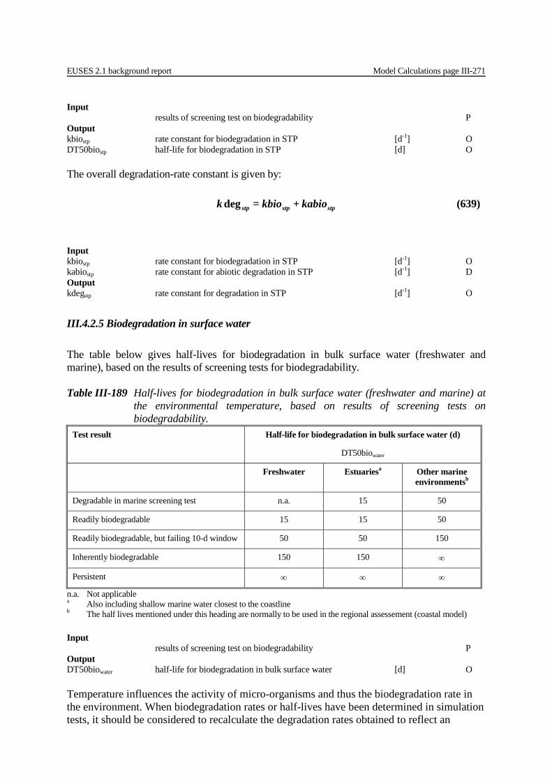
EUSES 2.1 background report Model Calculations page III-271
Input results of screening test on biodegradability P Output kbiostp rate constant for biodegradation in STP [d-1] O DT50biostp half-life for biodegradation in STP [d] O The overall degradation-rate constant is given by:
Input kbiostp rate constant for biodegradation in STP [d-1] O kabiostp rate constant for abiotic degradation in STP [d-1] D Output kdegstp rate constant for degradation in STP [d-1] O
III.4.2.5 Biodegradation in surface water The table below gives half-lives for biodegradation in bulk surface water (freshwater and marine), based on the results of screening tests for biodegradability.
n.a. Not applicable a Also including shallow marine water closest to the coastline b The half lives mentioned under this heading are normally to be used in the regional assessement (coastal model) Input results of screening test on biodegradability P Output DT50biowater half-life for biodegradation in bulk surface water [d] O Temperature influences the activity of micro-organisms and thus the biodegradation rate in the environment. When biodegradation rates or half-lives have been determined in simulation tests, it should be considered to recalculate the degradation rates obtained to reflect an
stpstpstp kabio+ kbio= k deg (639)
Table III-189 Half-lives for biodegradation in bulk surface water (freshwater and marine) at the environmental temperature, based on results of screening tests on biodegradability.
Test result Half-life for biodegradation in bulk surface water (d)
DT50biowater
Freshwater Estuariesa Other marine environmentsb
Degradable in marine screening test n.a. 15 50
Readily biodegradable 15 15 50
Readily biodegradable, but failing 10-d window 50 50 150
Inherently biodegradable 150 150 ∞
Persistent ∞ ∞ ∞

Model Calculations page III-272 EUSES 2.1 background report
average EU outdoor temperature by the following equation: ( )( )TEMPenvTEMPtest
testtempwaterenvtempwater e bioDT= bioDT −⋅⋅ 08.0__ 5050 (640)
Input DT50biowater_temp test half-life for biodegradation in water at temperature of the data set [d] S TEMPtest temperature of the measured data in simulation test [K] S TEMP environmental temperature [K] D Output DT50biowater_temp env half-life for biodegradation in water at the environmental temp. [d] O Values for the half-life (DT50) for biodegradation can be converted to first order rate constants for biodegradation.
Input DT50biowater half-life for biodegradation in bulk surface water [d] O DT50biowater_temp env half-life for biodegradation in water at the environmental temp. [d] O Output kbiowater rate constant for biodegradation in bulk surface water [d-1] O
III.4.2.6 Overall rate constant for degradation in bulk surface water The rate constants for the various different transformation processes can be summed into one overall degradation rate constant (used for regional and continental calculations only). It should be noted that different types of degradation (primary and ultimate) are added, which is done for modelling purposes only.
Input khydrwater rate constant for hydrolysis in surface water [d-1] O kphotowater rate constant for photolysis in surface water [d-1] O kbiowater rate constant for biodegradation in bulk surface water [d-1] O Output kdegwater total rate constant for degradation in bulk surface water [d-1] O
bioDT
= kbioorbioDT = kbio
envtempwaterwater
waterwater
_502ln
502ln (641)
waterwaterwaterwater kbio+ kphoto+ khydr= k deg (642)
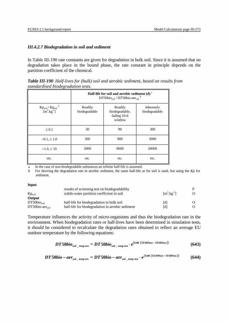
EUSES 2.1 background report Model Calculations page III-273
III.4.2.7 Biodegradation in soil and sediment In Table III-190 rate constants are given for degradation in bulk soil. Since it is assumed that no degradation takes place in the bound phase, the rate constant in principle depends on the partition coefficient of the chemical. Table III-190 Half-lives for (bulk) soil and aerobic sediment, based on results from standardised biodegradation tests.
Half-life for soil and aerobic sediment (d) a DT50biosoil / DT50bio-aersed b
Kpsoil / Kpsed b [m3.kg-1]
Readily biodegradable
Readily biodegradable,
failing 10-d window
Inherently biodegradable
≤ 0.1 30 90 300
>0.1, ≤ 1.0 300 900 3000
>1.0, ≤ 10 3000 9000 30000
etc. etc. etc. etc.
a In the case of non-biodegradable substances an infinite half-life is assumed. b For deriving the degradation rate in aerobic sediment, the same half-life as for soil is used, but using the Kp for
sediment. Input results of screening test on biodegradability P Kpsoil solids-water partition coefficient in soil [m3.kg-1] O Output DT50biosoil half-life for biodegradation in bulk soil [d] O DT50bio-aersed half-life for biodegradation in aerobic sediment [d] O Temperature influences the activity of micro-organisms and thus the biodegradation rate in the environment. When biodegradation rates or half-lives have been determined in simulation tests, it should be considered to recalculate the degradation rates obtained to reflect an average EU outdoor temperature by the following equations: ( )( )TEMPenvTEMPtest
testtempsoilenvtempsoil e bioDT= bioDT −⋅⋅ 08.0__ 5050 (643)
( )( )TEMPenvTEMPtest
testtempsedenvtempsed e aerbioDT= aerbioDT −⋅⋅−− 08.0__ 5050 (644)
Model Calculations page III-274 EUSES 2.1 background report
Input DT50biosoil_temp test half-life for biodegradation in soil at temperature of data set [d] S DT50bio-aersed_temp test half-life for biodeg. in aerobic sediment at temperature of data set [d] O TEMPtest temperature of the measured data in simulation test [K] S TEMP environmental temperature [K] D Output DT50biosoil_temp env half-life for biodegradation in soil at the environmental temp. [d] O DT50bio-aersed_temp env half-life for biodeg. in aerobic sediment at environmental temp. [d] O The following equation converts the DT50 to a rate constant for biodegradation in bulk soil. A rate constant for abiotic degradation (if known) is added.
Input DT50biosoil half-life for biodegradation in bulk soil [d] O DT50biosoil_temp env half-life for biodegradation in soil at the environmental temp. [d] O kabiosoil rate constant for abiotic degradation in bulk soil [d-1] D kbiosoil rate constant for biodegradation in bulk soil [d-1] O Output kdegsoil total rate constant for degradation in bulk soil [d-1] O The extrapolation of test results to rate constants for sediment is problematic, given the fact that sediment generally consists of a relatively thin oxic top layer and anoxic deeper layers. For the degradation in the anoxic layers, a rate constant of zero (infinite half-life) is assumed unless specific information on degradation under anaerobic conditions is available. For the oxic zone, the same rate constant and temperature correction as that for soil is assumed (see Table III-190).
Input DT50bio-aersed half-life for biodegradation in aerobic sediment [d] O DT50bio-aersed_temp env half-life for biodeg. in aerobic sediment at environmental temp. [d] O Faersed fraction of sediment compartment that is aerated [m3.m-3] D kabiosed rate constant for abiotic degradation in bulk sediment [d-1] D kbio-anaersed rate constant for anaerobic biodegradation in sediment [d-1] D Output kbio-aersed rate constant for biodegradation in aerobic sediment [d-1] O kdegsed total rate constant for degradation in bulk sediment [d-1] O
envtempsoil
soilsoil
soil bioDT = kbioor
bioDT = kbio
_502ln
502ln (645)
soilsoilsoil kabio + kbio= k deg (646)
envtempsed
sed-aersed
sed-aer aerbioDT = kbioor
aerbioDT = kbio
_502ln
502ln
−− (647)
sedsedsedsedsedsed kabio+ anaerkbio )Faer( + aerkbioFaerdegk −⋅−−⋅= 1 (648)
EUSES 2.1 background report Model Calculations page III-275
III.4.3 Sewage treatment Emissions to wastewater are treated in a sewage treatment plant (STP). For estimation of fate in an STP, the model SimpleTreat 3.1is used, which differs from version 3.0 only with respect to the default calculation of the solids-water partitioning coefficient Kp. This model is not described in detail in this section. For details and the mathematical process descriptions, the reader is referred to the SimpleTreat reference manual (Struijs, 1996). Sewage treatment takes place at the local, regional and continental scale. The definition of STP characteristics is the same at each of these spatial scales. The number of inhabitants is used to scale the size of the STP. The following options are included in the STP module: • temperature dependence of biodegradation, • Monod degradation kinetics, • not considering a primary settler (this 'six-box option' can only be specified at the local
spatial scale). Input: chemical properties HENRY Henry's law constant [Pa.m3.mol-1] kdegstp total rate constant for degradation in STP [d-1] KpRS solids-water partition coeff. in raw sewage sludge [m3.kg-1] KpPS solids-water partition coeff. in settled sewage sludge [m3.kg-1] KpA solids-water partition coeff. in activated sewage sludge [m3.kg-1] KpSLS solids-water partition coeff. in effluent sewage sludge [m3.kg-1] Input: emissions Elocalwater local emission rate to wastewater during episode [kgc.d-1] Eregwater regional emission rate to wastewater (annual average) [kgc.d-1] Econtwater continental emission rate to wastewater (annual average) [kgc.d-1] Intermediate results EFFLUENTlocalstp effluent discharge rate of local STP [m3.d-1] c Fstpi fraction directed to compartment i by local STP [-] Fstp-regi fraction directed to compartment i by regional STP [-] Fstp-conti fraction directed to compartment i by continental STP [-] i ∈ {air,water,sludge,degr} Output: local Estpair local indirect emission to air from STP during episode [kgc.d-1] Clocaleff concentration of chemical (total) in the STP effluent [kgc.m-3] Csludge concentration in dry sewage sludge [kgc.kg-1] PECstp PEC for micro-organisms in STP [kgc.m-3] Output: regional Estp-regair regional indirect emission to air from STP [kgc.d-1] Estp-regwater regional indirect emission to surface water from STP [kgc.d-1] Estp-regagric regional indirect emission to agricultural soil via sludge [kgc.d-1] Output: continental Estp-contair continental indirect emission to air from STP [kgc.d-1] Estp-contwater continental indirect emission to surface water from STP [kgc.d-1] Estp-contagric continental indirect emission to agricultural soil via sludge [kgc.d-1]
Model Calculations page III-276 EUSES 2.1 background report
Table III-191 lists the fixed parameters, subdivided into the categories raw sewage, primary sedimentation (9-box only), aerator and solids-liquid separation.
Only four parameters may be specified if the user does not accept the default values (see Table III-192). The sludge loading-rate parameter, kSLR (kg BOD kgdwt
-1 d-1), is chosen instead of the sludge retention time, SRT (d), to quantify the BOD loading of the installation. In principle, the hydraulic retention time, HRT (hr), could also have been chosen for this purpose. For the operation range relevant for wastewater treatment technology, these three parameters are interdependent according to certain relationships, which in some cases are empirical.
Table III-191 Fixed parameters for raw sewage and the operation of domestic wastewater treatment.
Parameter Symbol Unit Value
raw sewage
Mass of O2-binding material per person per day BOD [kgO2.eq-1.d-1] 0.054
Dry weight of solids produced per person per day SOLIDS [kgdwt.eq.-1 d-1] 0.09
Density of solids RHORS [kgdwt.m-3] 1500
primary settler (9-box only)
Depth DEPTHPS [m] 4
Hydraulic retention time (2 hours) HRTPS [d] 0.083
Density of suspended and settled solids RHOPS [kgdwt.m-3] 1500
activated sludge tank
Depth DEPTHA [m] 3
Density solids of activated sludge RHOA [kgdwt.m-3] 1300
Concentration solids of activated sludge CAS [kgdwt.m-3] 4
Steady-state O2 concentration in activated sludge COX [kg.m-3] 0.002
Aeration rate of bubble aeration G [m3.d-1.eq-1] 1.13
solids-liquid separator
Depth DEPTHSLS [m] 3
Density of suspended and settled solids RHOSLS [kgdwt.m-3] 1300
Concentration of solids in effluent SUSPeff [kgdwt.m-3] 0.03
Hydraulic retention time (6 hours) HRTSLS [d] 0.25
EUSES 2.1 background report Model Calculations page III-277
III.4.3.1 STP calculations The SimpleTreat calculations yield the following input-output: Input HENRY Henry's law constant [Pa.m3.mol-1] O kdegstp rate constant for biodegradation in STP [d-1] O Elocalwater local emission rate to wastewater during episode [kgc.d-1] O Eregwater regional emission rate to wastewater (annual average) [kgc.d-1] O Econtwater continental emission rate to wastewater (annual average) [kgc.d-1] O KpRS solids-water partition coeff. in raw sewage sludge [m3.kg-1] O KpPS solids-water partition coeff. in settled sewage sludge [m3.kg-1] O KpA solids-water partition coeff. in activated sewage sludge [m3.kg-1] O KpSLS solids-water partition coeff. in effluent sewage sludge [m3.kg-1] O Output Clocaleff concentration of chemical (total) in STP effluent [kgc.m-3] O Csludge concentration in dry sewage sludge [kgc.kgdwt
-1] O Fstpi fraction of emission directed to compartment i by STP [-] O Fstp-regi fraction directed to compartment i by regional STP [-] O Fstp-conti fraction directed to compartment i by continental STP [-] O i ∈ {air,water,sludge,degr} EUSES will perform a check whether the effluent concentration (Clocaleff) exceeds the water solubility. If this is the case, the results of this module should be studied in more detail on a case-by-case basis.
III.4.3.2 Calculation of influent concentration The influent concentration is used for exposure of micro-organisms in the case of intermittent release. For local-scale assessments, it is assumed that one point source is releasing its wastewater to one STP. The concentration in the influent of the STP, i.e. the untreated
Table III-192 Input parameters characterising size and mode of operation of sewage treatment plant.
Parameter Symbol Units Value
Sewage flow Qstp [m3.eq-1.d-1] 0.2
Number of inhabitants feeding system at scale local region EU
Nlocal N *
[eq] 10000 20.106 370.106
Sludge-loading rate kSLR [kgBOD.kgdwt-1.d-1] 0.15
Temperature of air above aeration tank (15 °C) TEMPstpair [K] 288
Temperature of water in aeration tank (15 °C) TEMPstpwater [K] 288
Wind speed (3 m/s) WINDSPEED [m.d-1] 2.59.105
Mode of aeration: surface (s) or bubble aeration (b) M [-] s
* Different parameter value possible on regional and continental scale.
Model Calculations page III-278 EUSES 2.1 background report
wastewater, can be calculated from the local emission to wastewater and the influent discharge of the STP. The influent discharge equals the effluent discharge.
Input Elocalwater local emission rate to wastewater during episode [kgc.d-1] O EFFLUENTlocalstp effluent discharge rate of local STP [m3.d-1] Oc
Fstpwater fraction of the emission to wastewater directed to effluent [-] O Output Clocalinf concentration in untreated wastewater [kgc.m-3] O Clocaleff concentration of chemical in the STP effluent [kgc.m-3] O For calculating the PEC in surface water (fresh water or marine water) without sewage treatment, the fraction of the emission to wastewater directed to effluent (Fstpwater) should be set to 1. The fractions to air and sludge (Fstpair and Fstpsludge, respectively) should be set to zero. This (Fstpwater=1) is the default for local emissions to the marine environment. The effluent discharge of the local STP is given by the following equation. The effluent discharges of the regional and continental STPs are given in Section III.4.4.5 (Equation 127 and 119 MOET DIT NIET ZIJN 655 and 656????). It should be noted that measured effluent-discharge rates cannot be entered directly by the user, but have to be derived by adjusting the number of inhabitants and the sewage flow per inhabitant.
Input Nlocal capacity of the local STP, number of inhabitants [eq] D Qstp sewage flow per inhabitant [m3.d-1.eq-1] D Output EFFLUENTlocalstp effluent discharge rate of local STP [m3.d-1] Oc
III.4.3.3 PEC for micro-organisms in STP For the risk characterisation of a chemical for micro-organisms in the STP, ideally the concentration in the aeration tank should be used. Assuming homogeneous mixing in the aeration tank, the dissolved concentration of a substance there is equal to the effluent concentration:
calEFFLUENTlo
Elocal= Clocalstp
waterinf (649)
watereff FstpClocal= Clocal ⋅inf (650)
QNlocalcalEFFLUENTlo stpstp ⋅= (651)
Clocal= PEC effstp (652)

EUSES 2.1 background report Model Calculations page III-279
Input Clocaleff total concentration of chemical in STP effluent [kgc.m-3] O Output PECstp PEC for micro-organisms in STP [kgc.m-3] O However, in the case of intermittent release, the concentration in of STP influent is more representative because the highest concentration as a result of shock load is accounted for.
Input Clocalinf total concentration of chemical in STP influent [kgc.m-3] O Output PECstp PEC for micro-organisms in STP [kgc.m-3] O
III.4.3.4 Calculation of the emission to air from the STP The (indirect) emission from the STP to air is given by the fraction of the emission to wastewater, directed to air.
Input Fstpair fraction of emission to air from STP [-] O Elocalwater local emission rate to wastewater during emission episode [kgc.d-1] O Output Estpair local emission to air from STP during emission episode [kgc.d-1] O
III.4.3.5 Emissions from STP at the regional and continental scale The indirect emissions via the STP at the regional and continental scale are calculated from the emissions to wastewater and the fate in the STP. The relative fate (expressed as fractions redirected to air, water and sludge) will usually be identical at all three spatial scales. However, when the degradation in the STP is modelled by Monod kinetics, differences in fate are possible.
Clocal= PEC infstp (653)
waterairair ElocalFstp=Estp ⋅ (654)
Ereg reg-= Fstp reg-Estp waterii ⋅ (655)
ic}sludge/agrwater,{air, i
Econt cont-= Fstp cont-Estp waterii
∈
⋅ (656)

Model Calculations page III-280 EUSES 2.1 background report
Input Fstp-regi fraction directed to compartment i by regional STP [-] O Fstp-conti fraction directed to compartment i by continental STP [-] O Eregwater regional emission rate to wastewater [kgc.d-1] O Econtwater continental emission rate to wastewater [kgc.d-1] O Output Estp-regair regional emission to air from STP [kgc.d-1] O Estp-regwater regional emission to water from STP [kgc.d-1] O Estp-regagric regional emission to agricultural soil via sludge [kgc.d-1] O Estp-contair continental emission to air from STP [kgc.d-1] O Estp-contwater continental emission to water from STP [kgc.d-1] O Estp-contagric continental emission to agricultural soil via sludge [kgc.d-1] O

EUSES 2.1 background report Model Calculations page III-281
III.4.4 Regional environmental distribution Steady-state exposure concentrations at the regional and continental scales are calculated for all environmental compartments using a nested version of the multi-media fate model SimpleBox (Van de Meent, 1993; Brandes et al., 1996; see also Section 2.4.4). The version of SimpleBox implemented in EUSES is described in technical detail by den Hollander, van de Meent and van Eijkeren (2003, in prep.) In this section, the regional model is described by its inputs, outputs and default values. Furthermore, the calculations for the net sedimentation rate and the residence time in air and water are given (these are shown as closed outputs in the defaults section of the EUSES programme). Input: regional emissions Eregj direct emission to compartment j (annual average flux) [kgc.d-1] j ∈ {direct-water,ind,agric,air} Estp-regj regional indirect emission to compartment j from STP [kgc.d-1] j ∈ {water,agric,air} Input: continental emissions Econtj direct emission to compartment j (annual average flux) [kgc.d-1] j ∈ {direct-water,ind,agric,air} Estp-contj continental indirect emission to compartment j from STP [kgc.d-1] j ∈ {water,agric,air} Input: chemical properties Kow octanol-water partition coefficient [S] (only for estimation of BCF for aquatic biota) Fassaer fraction of chemical associated with aerosol particles [-] Kair-water air-water partition coefficient [m3.m-3] c Ksoil-water soil-water partition coefficient [m3.m-3] c Ksed-water sediment-water partition coefficient [m3.m-3] c Kpsusp solids-water partition coefficient in suspended matter [m3.kgsolids
-1] RHOsoil wet bulk density of soil [kgwwt.m-3] c kdegair rate constant for degradation in air [d-1] kdegwater rate constant for degradation in bulk water [d-1] kdegsoil rate constant for degradation in bulk soil [d-1] kdegsed rate constant for degradation in bulk sediment [d-1] Output: continental concentrations PECcontwater,tot continental PEC in surface water (total) [kgc.m-3] c PECcontwater continental PEC in surface water (dissolved) [kgc.m-3] c PECcontair continental PEC in air (total) [kgc.m-3] c PECcontagric continental PEC in agricultural soil (total) [kgc.kgwwt
-1] c PECcontagric,porew continental PEC in pore water of agricultural soils [kgc.m-3] c PECcontnatural continental PEC in natural soil (total) [kgc.kgwwt
-1] c PECcontind continental PEC in industrial soil (total) [kgc.kgwwt
-1] c PECcontsed continental PEC in sediment (total) [kgc.kgwwt
-1] c Output: regional concentrations PECregwater,tot regional PEC in surface water (total) [kgc.m-3] PECregwater regional PEC in surface water (dissolved) [kgc.m-3] PECregair regional PEC in air (total) [kgc.m-3] PECregagric regional PEC in agricultural soil (total) [kgc.kgwwt
-1] PECregagric,porew regional PEC in pore water of agricultural soil [kgc.m-3] PECregnatural regional PEC in natural soil (total) [kgc.kgwwt
-1] PECregind regional PEC in industrial soil (total) [kgc.kgwwt
-1] PECregsed regional PEC in sediment (total) [kgc.kgwwt
-1]
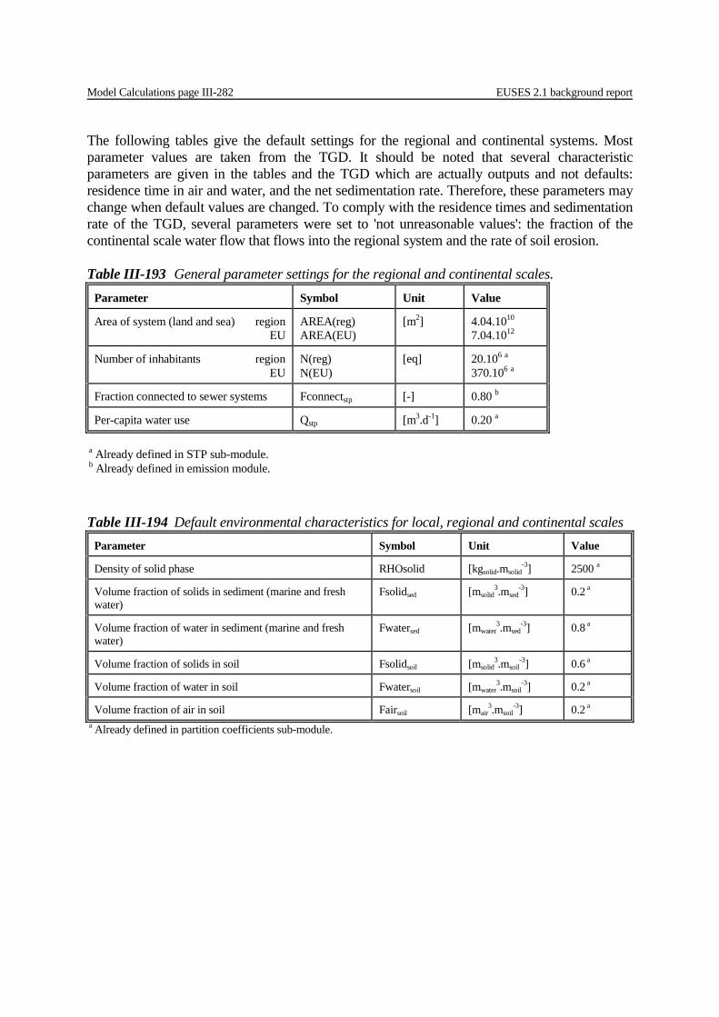
Model Calculations page III-282 EUSES 2.1 background report
The following tables give the default settings for the regional and continental systems. Most parameter values are taken from the TGD. It should be noted that several characteristic parameters are given in the tables and the TGD which are actually outputs and not defaults: residence time in air and water, and the net sedimentation rate. Therefore, these parameters may change when default values are changed. To comply with the residence times and sedimentation rate of the TGD, several parameters were set to 'not unreasonable values': the fraction of the continental scale water flow that flows into the regional system and the rate of soil erosion.
Table III-193 General parameter settings for the regional and continental scales. Parameter Symbol Unit Value
Area of system (land and sea) region EU
AREA(reg) AREA(EU)
[m2] 4.04.1010 7.04.1012
Number of inhabitants region EU
N(reg) N(EU)
[eq] 20.106 a 370.106 a
Fraction connected to sewer systems Fconnectstp [-] 0.80 b
Per-capita water use Qstp [m3.d-1] 0.20 a
a Already defined in STP sub-module. b Already defined in emission module.
Table III-194 Default environmental characteristics for local, regional and continental scales Parameter Symbol Unit Value
Density of solid phase RHOsolid [kgsolid.msolid-3] 2500 a
Volume fraction of solids in sediment (marine and fresh water)
Fsolidsed [msolid3.msed
-3] 0.2 a
Volume fraction of water in sediment (marine and fresh water)
Fwatersed [mwater3.msed
-3] 0.8 a
Volume fraction of solids in soil Fsolidsoil [msolid3.msoil
-3] 0.6 a
Volume fraction of water in soil Fwatersoil [mwater3.msoil
-3] 0.2 a
Volume fraction of air in soil Fairsoil [mair3.msoil
-3] 0.2 a a Already defined in partition coefficients sub-module.

EUSES 2.1 background report Model Calculations page III-283
Table III-195 Parameter settings for regional and continental air. Parameter Symbol Unit Value
Atmospheric mixing height HEIGHTair [m] 1000
Wind speed of system WINDSPEED [m.d-1] 2.59.105 a
Residence time of air region continent
TAUair * [d] 0.687 Oc 9.05 Oc
Aerosol-deposition velocity DEPRATEaer [m.d-1] 86.4
Aerosol-collection efficiency COLLEFFaer [-] 2.105
Average daily precipitation RAINRATE [m.d-1] 1.92.10-3
a Already defined in STP sub-module. * Different parameter value possible on regional and continental scale.
Table III-196 Parameter settings for regional and continental marine and fresh waters. Parameter Symbol Unit Value
Area fraction of fresh water region (both 3% of land area) continent
Fwater * [-] 0.0297 0.015
Area fraction of marine water region continent
Fwater,marine * [-] 0.0099 0.5
Water depth fresh water region+cont. DEPTHwater * [m] 3
Water depth marine region continent
DEPTHwater, marine * [m] 10 200
Fraction of flow from region larger scale continent
Fflowout * [-] 0.034 0
Residence time of fresh water region continent
TAUwater *
[d] 43.3 Oc 1721 Oc
Residence time of marine water region continent
TAUwater, marine *
[d] 4.04 Oc 365 Oc
Suspended-solids conc. region+cont.
SUSPwater * [kgdwt.m-3] 0.015 .
Suspended-solids conc. region+cont. SUSPwater, marine * [kgdwt.m-3] 0.005
Concentration of biota (marine and fresh water)
BIOTAwater [kgwwt.m-3] 0.001
Fraction of rainwater infiltrating in soil Finfsoil [-] 0.25 a
Rate of wet precipitation (700 mm/year) RAINRATE [m.d-1] 1.92.10-3 a
* Different parameter value possible on regional and continental scale.

Model Calculations page III-284 EUSES 2.1 background report
Table III-197 Parameter settings for regional and continental marine and fresh water sediments.
Parameter Symbol Unit Value
Sediment mixing depth DEPTHsed [m] 0.03
Settling velocity of suspended solids SETTLRATEsusp [m.d-1] 2.5
(Biogenic) production of suspended solids in fresh water region: 10g.m-2.a-1 continent: 10g.m-2.a-1
SUSPPRODwater *
[kg.d-1]
3.3.104 Oc 2.9.106 Oc
(Biogenic) production of suspended solids in marine water region: 10g.m-2.a-1 continent: 5g.m-2.a-1
SUSPPRODwater, marine *
[kg.d-1]
1.1.104 Oc 4.8.107 Oc
Suspended solids in STP effluent SUSPeff [kgdwt.m-3] 0.030 a
Net sedimentation rate fresh water region continent
NETsedrate * [msed.d-1] 7.5.10-6 Oc 7.5.10-6 Oc
Net sedimentation rate marine water region continent
NETsedratemarine * [msed.d-1] 4.2.10-6 Oc 1.8.10-8 Oc
a Already defined in STP sub-module. * Different parameter value possible on regional and continental scale.
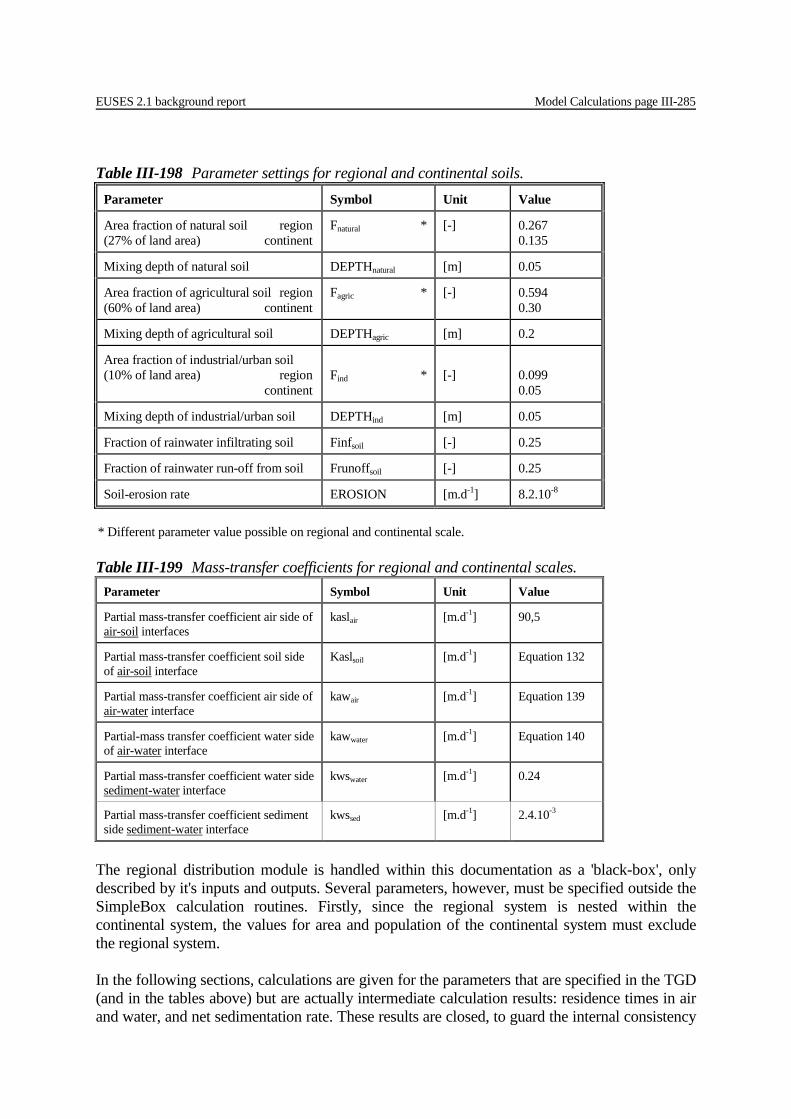
EUSES 2.1 background report Model Calculations page III-285
The regional distribution module is handled within this documentation as a 'black-box', only described by it's inputs and outputs. Several parameters, however, must be specified outside the SimpleBox calculation routines. Firstly, since the regional system is nested within the continental system, the values for area and population of the continental system must exclude the regional system. In the following sections, calculations are given for the parameters that are specified in the TGD (and in the tables above) but are actually intermediate calculation results: residence times in air and water, and net sedimentation rate. These results are closed, to guard the internal consistency
Table III-198 Parameter settings for regional and continental soils. Parameter Symbol Unit Value
Area fraction of natural soil region (27% of land area) continent
Fnatural * [-] 0.267 0.135
Mixing depth of natural soil DEPTHnatural [m] 0.05
Area fraction of agricultural soil region (60% of land area) continent
Fagric * [-] 0.594 0.30
Mixing depth of agricultural soil DEPTHagric [m] 0.2
Area fraction of industrial/urban soil (10% of land area) region continent
Find *
[-]
0.099 0.05
Mixing depth of industrial/urban soil DEPTHind [m] 0.05
Fraction of rainwater infiltrating soil Finfsoil [-] 0.25
Fraction of rainwater run-off from soil Frunoffsoil [-] 0.25
Soil-erosion rate EROSION [m.d-1] 8.2.10-8
* Different parameter value possible on regional and continental scale.
Table III-199 Mass-transfer coefficients for regional and continental scales. Parameter Symbol Unit Value
Partial mass-transfer coefficient air side of air-soil interfaces
kaslair [m.d-1] 90,5
Partial mass-transfer coefficient soil side of air-soil interface
Kaslsoil [m.d-1] Equation 132
Partial mass-transfer coefficient air side of air-water interface
kawair [m.d-1] Equation 139
Partial-mass transfer coefficient water side of air-water interface
kawwater [m.d-1] Equation 140
Partial mass-transfer coefficient water side sediment-water interface
kwswater [m.d-1] 0.24
Partial mass-transfer coefficient sediment side sediment-water interface
kwssed [m.d-1] 2.4.10-3
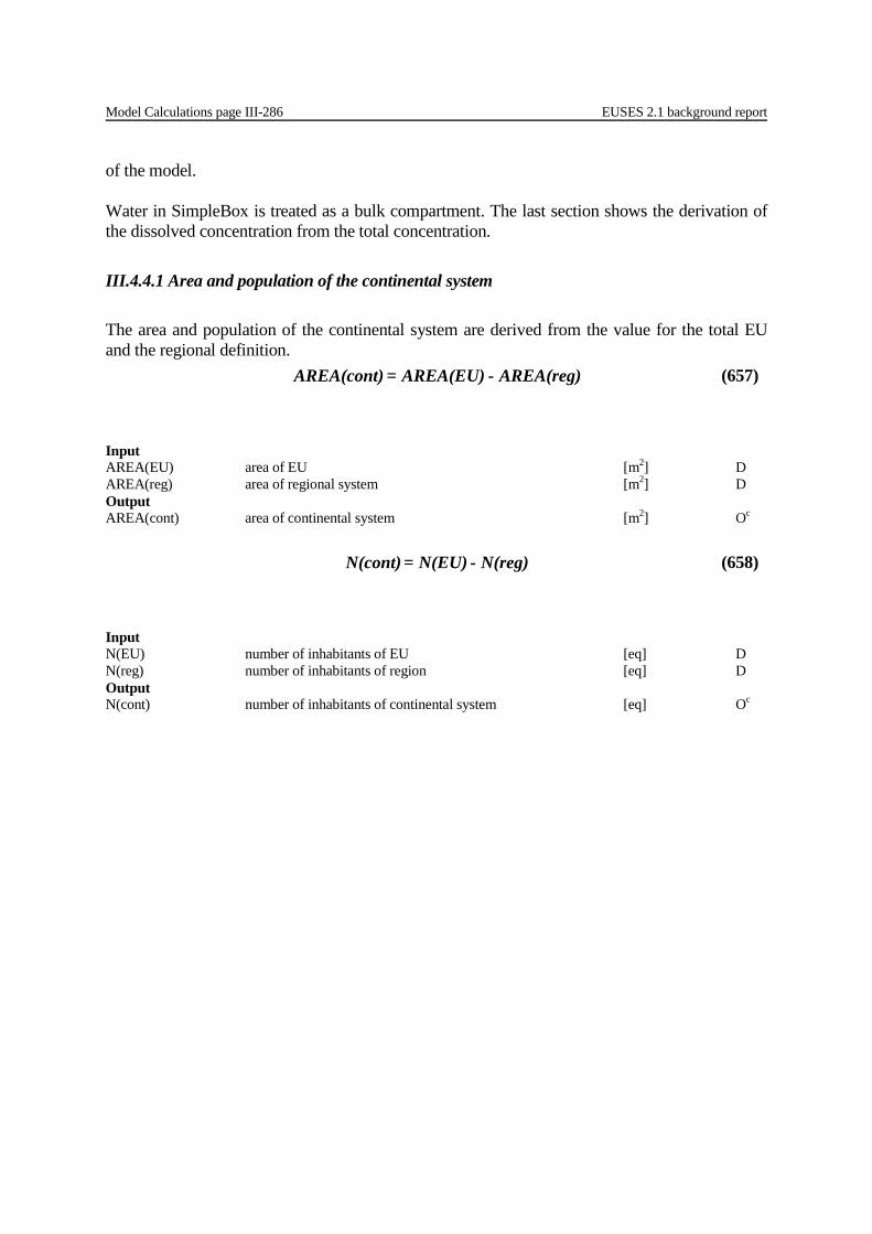
Model Calculations page III-286 EUSES 2.1 background report
of the model. Water in SimpleBox is treated as a bulk compartment. The last section shows the derivation of the dissolved concentration from the total concentration.
III.4.4.1 Area and population of the continental system The area and population of the continental system are derived from the value for the total EU and the regional definition.
Input AREA(EU) area of EU [m2] D AREA(reg) area of regional system [m2] D Output AREA(cont) area of continental system [m2] Oc
Input N(EU) number of inhabitants of EU [eq] D N(reg) number of inhabitants of region [eq] D Output N(cont) number of inhabitants of continental system [eq] Oc
AREA(reg) -AREA(EU)= AREA(cont) (657)
N(reg) -N(EU)= N(cont) (658)
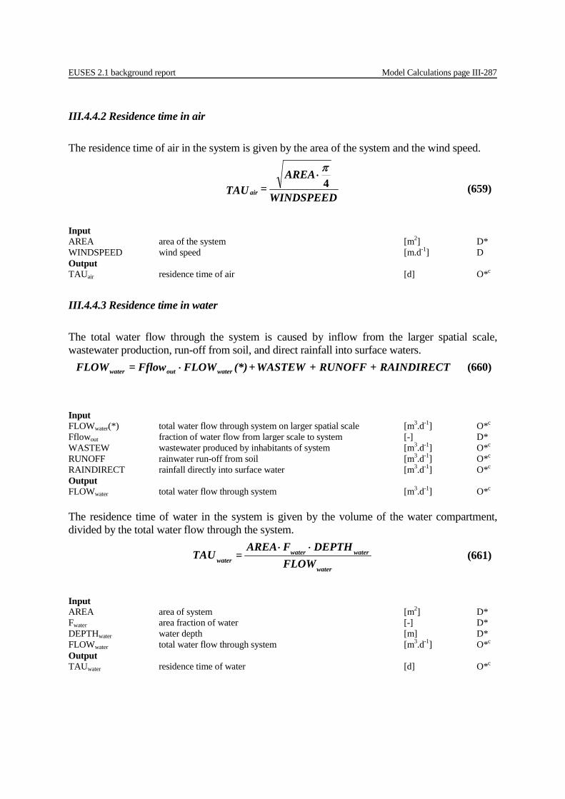
EUSES 2.1 background report Model Calculations page III-287
III.4.4.2 Residence time in air The residence time of air in the system is given by the area of the system and the wind speed.
Input AREA area of the system [m2] D* WINDSPEED wind speed [m.d-1] D Output TAUair residence time of air [d] O*c
III.4.4.3 Residence time in water The total water flow through the system is caused by inflow from the larger spatial scale, wastewater production, run-off from soil, and direct rainfall into surface waters.
Input FLOWwater(*) total water flow through system on larger spatial scale [m3.d-1] O*c Fflowout fraction of water flow from larger scale to system [-] D* WASTEW wastewater produced by inhabitants of system [m3.d-1] O*c RUNOFF rainwater run-off from soil [m3.d-1] O*c RAINDIRECT rainfall directly into surface water [m3.d-1] O*c Output FLOWwater total water flow through system [m3.d-1] O*c The residence time of water in the system is given by the volume of the water compartment, divided by the total water flow through the system.
Input AREA area of system [m2] D* Fwater area fraction of water [-] D* DEPTHwater water depth [m] D* FLOWwater total water flow through system [m3.d-1] O*c Output TAUwater residence time of water [d] O*c
WINDSPEED
AREA= TAU air
4π⋅
(659)
RAINDIRECT + RUNOFF + WASTEW+ (*)FLOW Fflow= FLOW wateroutwater ⋅ (660)
water
waterwaterwater FLOW
DEPTHFAREA= TAU
⋅⋅ (661)
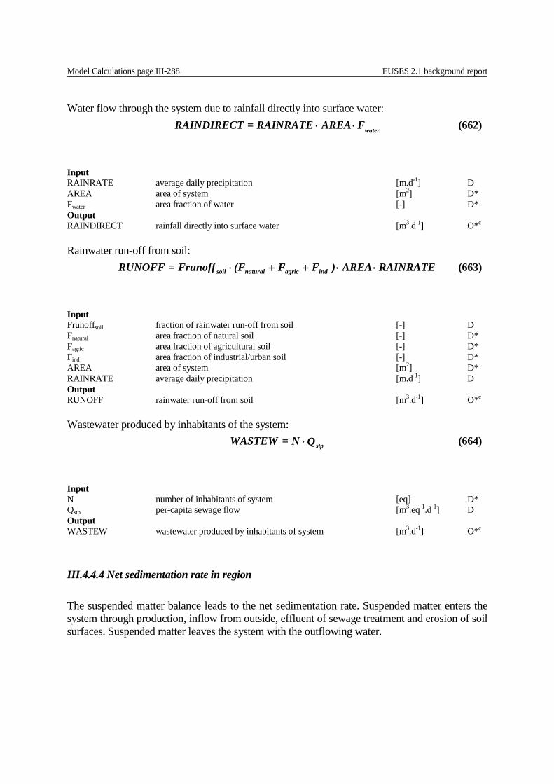
Model Calculations page III-288 EUSES 2.1 background report
Water flow through the system due to rainfall directly into surface water:
Input RAINRATE average daily precipitation [m.d-1] D AREA area of system [m2] D* Fwater area fraction of water [-] D* Output RAINDIRECT rainfall directly into surface water [m3.d-1] O*c Rainwater run-off from soil:
Input Frunoffsoil fraction of rainwater run-off from soil [-] D Fnatural area fraction of natural soil [-] D* Fagric area fraction of agricultural soil [-] D* Find area fraction of industrial/urban soil [-] D* AREA area of system [m2] D* RAINRATE average daily precipitation [m.d-1] D Output RUNOFF rainwater run-off from soil [m3.d-1] O*c Wastewater produced by inhabitants of the system:
Input N number of inhabitants of system [eq] D* Qstp per-capita sewage flow [m3.eq-1.d-1] D Output WASTEW wastewater produced by inhabitants of system [m3.d-1] O*c
III.4.4.4 Net sedimentation rate in region The suspended matter balance leads to the net sedimentation rate. Suspended matter enters the system through production, inflow from outside, effluent of sewage treatment and erosion of soil surfaces. Suspended matter leaves the system with the outflowing water.
waterF AREA RAINRATE= RAINDIRECT ⋅⋅ (662)
RAINRATE AREA )FF (FFrunoff= RUNOFF indagricnaturalsoil ⋅⋅++⋅ (663)
Q N= WASTEW stp⋅ (664)
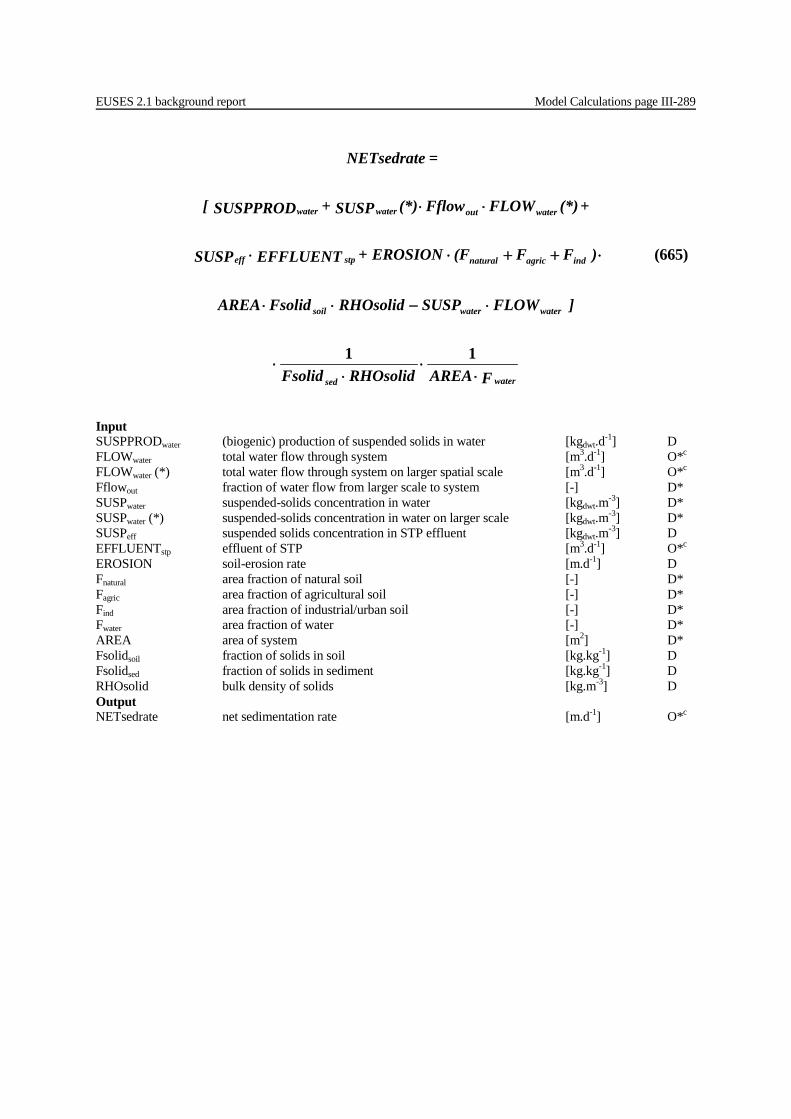
EUSES 2.1 background report Model Calculations page III-289
Input SUSPPRODwater (biogenic) production of suspended solids in water [kgdwt.d-1] D FLOWwater total water flow through system [m3.d-1] O*c FLOWwater (*) total water flow through system on larger spatial scale [m3.d-1] O*c Fflowout fraction of water flow from larger scale to system [-] D* SUSPwater suspended-solids concentration in water [kgdwt.m-3] D* SUSPwater (*) suspended-solids concentration in water on larger scale [kgdwt.m-3] D* SUSPeff suspended solids concentration in STP effluent [kgdwt.m-3] D EFFLUENTstp effluent of STP [m3.d-1] O*c EROSION soil-erosion rate [m.d-1] D Fnatural area fraction of natural soil [-] D* Fagric area fraction of agricultural soil [-] D* Find area fraction of industrial/urban soil [-] D* Fwater area fraction of water [-] D* AREA area of system [m2] D* Fsolidsoil fraction of solids in soil [kg.kg-1] D Fsolidsed fraction of solids in sediment [kg.kg-1] D RHOsolid bulk density of solids [kg.m-3] D Output NETsedrate net sedimentation rate [m.d-1] O*c
F AREA
RHOsolidFsolid
] FLOW SUSP RHOsolid Fsolid AREA
)FF (F EROSION + EFFLUENT SUSP
+ (*)FLOWFflow (*)SUSP + SUSPPROD [
= NETsedrate
watersed
waterwatersoil
indagricnaturalstpeff
wateroutwaterwater
⋅⋅
⋅⋅
⋅−⋅⋅
⋅++⋅⋅
⋅⋅
11
(665)

Model Calculations page III-290 EUSES 2.1 background report
III.4.4.5 Regional and continental effluent discharges The effluent discharge from regional and continental STPs depends on the fraction connected to treatment plants.
Input N number of inhabitants of system [eq] D* Qstp per-capita sewage flow [m3.eq-1.d-1] D Fconnectstp fraction connected to sewer systems [-] D Output EFFLUENTstp effluent of STP [m3.d-1] O*c
III.4.4.6 Calculation of the dissolved concentration in surface water In SimpleBox, water is treated as a bulk compartment, including biota and suspended matter. The model calculations therefore yield a total concentration in surface water. In subsequent calculations, and in risk characterisation, the dissolved concentration is required. Therefore, the total concentration is converted as follows. The bioconcentration factor for aquatic biota (BCFbiota) used in this equation to calculate the distribution over different phases is calculated from Equation (162/163). This parameter is closed and should be distinguished from BCFfish since measured BCF data for fish cannot be assumed representative for all aquatic biota. It should be noted that when a Kow value is not entered (e.g. for a metal), BCFbiota is set to zero. If sorption to aquatic biota is relevant for the dissolved concentration in surface water, the Kp for suspended matter can be adjusted manually to account for this process.
Input PECregwater,tot regional concentration in total surface water [kgc.m-3] O Kpsusp solids-water partition coefficient of suspended matter [m3.kgsolids
-1] O SUSPwater concentration of suspended matter in water of region [kgdwt.m-3] D BCFbiota BCF for aquatic biota in regional/continental model [m3.kgwwt
-1] Oc BIOTAwater concentration of aquatic biota in regional system [kgwwt.m-3] D Output PECregwater regional PEC in surface water [kgc.m-3] O
III.4.4.7 Calculation of porewater concentration in agricultural soil The concentration in porewater is derived from the total concentration by using the soil-water partition coefficient and the bulk density of the soil. The porewater concentration is used to estimate concentrations in plants and drinking water for indirect human exposure.
Fconnect Q N= EFFLUENT stpstpstp ⋅⋅ (666)
BIOTA BCF + SUSP Kp +
PECreg= PECreg
waterbiotawatersusp
totwater,water ⋅⋅1
(667)

EUSES 2.1 background report Model Calculations page III-291
Input PECregagric regional PEC in agricultural soil (total) [kgc.kgwwt
-1] O RHOsoil wet bulk density of soil [kgwwt.m-3] Oc Ksoil-water soil-water partition coefficient [m3.m-3] Oc Output PECregagric,porew regional PEC in porewater of agricultural soil [kgc.m-3] O
III.4.4.8 Mass transfer at air-soil and air-water interface on regional and continental scale Soil–air interface A substance-dependent soil-side partial mass transfer coefficient (PMTC) at the soil-air interface kaslsoil (m.d-1) is deduced from the exponential concentration profile in soil:
+=
p
soilsoilsoil d
DeffVeffkasl (669)
In soil, processes of downward advection (pore water + small particles), diffusion (air, water, solids), and degradation take place simultaneously. These processes are included in Simplebox 3.0 (Hollander et al., 2003). The result is an exponential decrease of the concentration with depth (Cz), characterised by a substance-dependent penetration depth (dp)
;/0
pdzz eCC −⋅=
soil
soilsoilsoilsoilp k
kDeffVeffVeffd
deg2deg2
⋅⋅++
= (670)
in which:
soilsoil
soilsoil Fsolid
soilSOLIDadvsoilFRsFwater
FRAINRATEsoilFRwVeff ...
inf. +
⋅= (671)
soilsoil
soil
soil
soilsoil Fsolid
soilSOLIDdiffsoilFRsFwater
FwaterDIFFwatersoilFRw
FairFairDIFFgas
soilFRaDeff .....5.15.1
⋅+⋅
+⋅
=
(672)
''.psoilsoilhsoil
soil
KFsolidFwaterKFairFwater
soilFRw⋅++⋅
= (673)
soilpsoilphsoil
soil
FsolidKFwaterKKFairFsolid
soilFRs++⋅
= '''. (674)
soilFRssoilFRwsoilFRa ..1. −−= (675)
K
RHO PECreg= PECreg
water-soil
soilporewagricporewagric,
⋅,
(668)
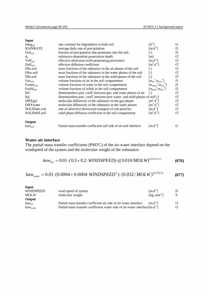
Model Calculations page III-292 EUSES 2.1 background report
Input kdegsoil rate constant for degradation in bulk soil [d-1] O RAINRATE average daily rate of precipitation [m.d-1] D Finfsoil fraction of precipitation that penetrates into the soil. [-] D dp substance-dependent penetration depth [m] Oc Veffsoil effective advection (with penetrating porewater) [m.d-1] Oc Deffsoil effective diffusion coefficient [m2.d-1] Oc FRa.soil mass fractions of the substance in the air phases of the soil [-] Oc FRw.soil mass fractions of the substance in the water phases of the soil [-] Oc FRs.soil mass fractions of the substance in the solid phases of the soil [-] Oc Fairsoil volume fractions of air in the soil compartment [mair
3.msoil-3] D
Fwatersoil volume fractions of water in the soil compartment [mwater3.msoil
-3] D Fsolidsoil volume fractions of solids in the soil compartment [msolid
3.msoil-3] D
Kh' dimensionless part. coeff. between gas- and water phases of air [-] Oc Kp' dimensionless part. coeff. between pore water- and solid phases of soil [-] Oc DIFFgas molecular diffusivity of the substance in the gas phases [m2.d-1] Oc DIFFwater molecular diffusivity of the substance in the water phases [m2.d-1] Oc SOLIDadv.soil rate of advective downward transport of soil particles [m.d-1] Oc SOLIDdiff.soil solid phase diffusion coefficient in the soil compartment [m2.d-1] Oc Output kaslsoil Partial mass-transfer coefficient soil side of air-soil interface [m.d-1] O Water-air interface The partial mass transfer coefficients (PMTC) of the air-water interface depend on the windspeed of the system and the molecular weight of the substance: ),,(
air /MOLW).((WINDSPEED)..(.kaw 5067001802030010 ⋅⋅⋅+⋅= (676)
)5,05,0(2 )/032.0()0004.00004.0(01.0 ⋅⋅⋅+⋅= MOLWWINDSPEEDkawwater (677)
Input WINDSPEED wind speed of system [m.d-1] D MOLW molecular weight [kgc.mol-1] S Output kawair Partial mass-transfer coefficient air side of air-water interface [m.d-1] O kawwater Partial-mass transfer coefficient water side of air-water interface[m.d-1] O

EUSES 2.1 background report Model Calculations page III-293
III.4.5 Local environmental distribution In this section, the calculation of local environmental concentrations (PEClocal) is presented. Dedicated models are used for the compartments air, surface water and soil. Concentrations in sediment and groundwater are derived from the concentrations in surface water and soil, respectively. It should be noted that these calculations are performed for each relevant application and each step of the life cycle. Several intermediate results of the soil sub-module are closed, since these results are too strictly model-related to allow for changes by the user (e.g. the concentration after 10 years due to deposition only: Cdep10i). Input: local direct emissions Elocalair local direct emission rate to air during episode [kgc.d-1] Temission number of days per year that emission takes place [d.year-1] Input: indirect emissions via STP Estpair local indirect emission to air from STP during episode [kgc.d-1] Clocaleff concentration of chemical in STP effluent [kgc.m-3] Csludge concentration in dry sewage sludge [kgc.kgdwt
-1] EFFLUENTlocalstp effluent discharge rate of local STP [m3.d-1] c Input: chemical properties Fassaer fraction of chemical bound to aerosol [-] Kair-water air-water partition coefficient [m3.m-3] c Ksoil-water soil-water partition coefficient [m3.m-3] c Ksusp-water suspended matter-water partition coefficient [m3.m-3] c Kpsusp solids-water partition coefficient of suspended matter [m3.kg-1] kdegsoil rate constant for degradation in soil [d-1] Input background concentrations PECregair regional concentration in air [kgc.m-3] PECregwater regional concentration in surface water [kgc.m-3] PECregwater,marine regional concentration in marine surface water [kgc.m-3] PECregnatural regional concentration in natural soil [kgc.kgwwt
-1] Intermediate results 1: removal rate constants soil kvolat i rate constant for volatilisation from soil i [d-1] kleach i rate constant for leaching from soil i [d-1] i ∈ {soil,agric,grassland} ki total rate constant for removal from topsoil i [d-1] Intermediate results 2 Clocalair local concentration in air during emission episode [kgc.m-3] Clocalair,ann annual average concentration in air, 100 m from point source [kgc.m-3] DEPtotal total deposition flux during emission episode [kgc.m-2.d-1] DEPtotalann annual average total deposition flux [kgc.m-2.d-1] Clocalwater local concentration in surface water during emission episode [kgc.m-3] Clocalwater,ann annual average local concentration in surface water [kgc.m-3] Clocalwater,marine local conc. in marine surface water during emission episode [kgc.m-3] Clocalwater,ann,marine annual average local concentration in marine surface water [kgc.m-3] Clocalsoil local concentration in agric. soil averaged over 30 days [kgc.kgwwt
-1] (to assess terrestrial ecosystem) Clocalagric local concentration in agric. soil averaged over 180 days [kgc.kgwwt
-1] (to calculate concentration in crops) Clocalgrassland local concentration in grassland averaged over 180 days [kgc.kgwwt
-1] Fst-sti fraction of steady-state situation achieved in soil i [-] c i ∈ {soil,agric,grassland} Output
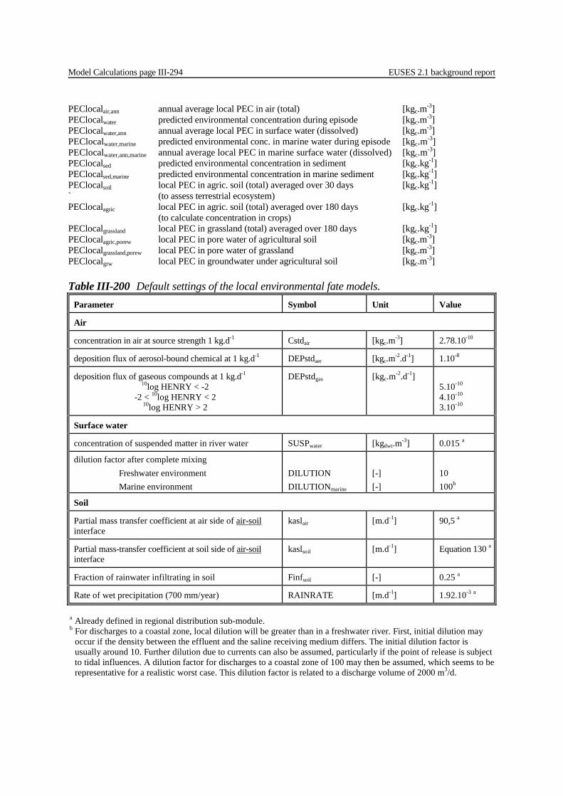
Model Calculations page III-294 EUSES 2.1 background report
PEClocalair,ann annual average local PEC in air (total) [kgc.m-3] PEClocalwater predicted environmental concentration during episode [kgc.m-3] PEClocalwater,ann annual average local PEC in surface water (dissolved) [kgc.m-3] PEClocalwater,marine predicted environmental conc. in marine water during episode [kgc.m-3] PEClocalwater,ann,marine annual average local PEC in marine surface water (dissolved) [kgc.m-3] PEClocalsed predicted environmental concentration in sediment [kgc.kg-1] PEClocalsed,marine predicted environmental concentration in marine sediment [kgc.kg-1] PEClocalsoil local PEC in agric. soil (total) averaged over 30 days [kgc.kg-1] ` (to assess terrestrial ecosystem) PEClocalagric local PEC in agric. soil (total) averaged over 180 days [kgc.kg-1] (to calculate concentration in crops) PEClocalgrassland local PEC in grassland (total) averaged over 180 days [kgc.kg-1] PEClocalagric,porew local PEC in pore water of agricultural soil [kgc.m-3] PEClocalgrassland,porew local PEC in pore water of grassland [kgc.m-3] PEClocalgrw local PEC in groundwater under agricultural soil [kgc.m-3]
Table III-200 Default settings of the local environmental fate models. Parameter Symbol Unit Value
Air
concentration in air at source strength 1 kg.d-1 Cstdair [kgc.m-3] 2.78.10-10
deposition flux of aerosol-bound chemical at 1 kg.d-1 DEPstdaer [kgc.m-2.d-1] 1.10-8
deposition flux of gaseous compounds at 1 kg.d-1 10log HENRY < -2
-2 < 10log HENRY < 2 10log HENRY > 2
DEPstdgas [kgc.m-2.d-1] 5.10-10 4.10-10 3.10-10
Surface water
concentration of suspended matter in river water SUSPwater [kgdwt.m-3] 0.015 a
dilution factor after complete mixing Freshwater environment Marine environment
DILUTION DILUTIONmarine
[-] [-]
10 100b
Soil
Partial mass transfer coefficient at air side of air-soil interface
kaslair [m.d-1] 90,5 a
Partial mass-transfer coefficient at soil side of air-soil interface
kaslsoil [m.d-1] Equation 130 a
Fraction of rainwater infiltrating in soil Finfsoil [-] 0.25 a
Rate of wet precipitation (700 mm/year) RAINRATE [m.d-1] 1.92.10-3 a
a Already defined in regional distribution sub-module. b For discharges to a coastal zone, local dilution will be greater than in a freshwater river. First, initial dilution may
occur if the density between the effluent and the saline receiving medium differs. The initial dilution factor is usually around 10. Further dilution due to currents can also be assumed, particularly if the point of release is subject to tidal influences. A dilution factor for discharges to a coastal zone of 100 may then be assumed, which seems to be representative for a realistic worst case. This dilution factor is related to a discharge volume of 2000 m3/d.
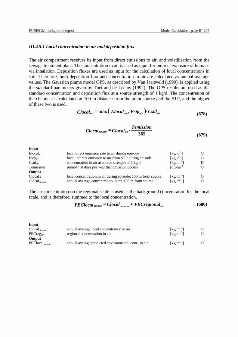
EUSES 2.1 background report Model Calculations page III-295
III.4.5.1 Local concentration in air and deposition flux The air compartment receives its input from direct emissions to air, and volatilisation from the sewage treatment plant. The concentration in air is used as input for indirect exposure of humans via inhalation. Deposition fluxes are used as input for the calculation of local concentrations in soil. Therefore, both deposition flux and concentration in air are calculated as annual average values. The Gaussian plume model OPS, as described by Van Jaarsveld (1990), is applied using the standard parameters given by Toet and de Leeuw (1992). The OPS results are used as the standard concentration and deposition flux at a source strength of 1 kg/d. The concentration of the chemical is calculated at 100 m distance from the point source and the STP, and the higher of these two is used.
Input Elocalair local direct emission rate to air during episode [kgc.d-1] O Estpair local indirect emission to air from STP during episode [kgc.d-1] O Cstdair concentration in air at source strength of 1 kg.d-1 [kgc.m-3] D Temission number of days per year that emission occurs [d.year-1] O Output Clocalair local concentration in air during episode, 100 m from source [kgc.m-3] O Clocalair,ann annual average concentration in air, 100 m from source [kgc.m-3] O The air concentration on the regional scale is used as the background concentration for the local scale, and is therefore, summed to the local concentration.
Input Clocalair,ann annual average local concentration in air [kgc.m-3] O PECregair regional concentration in air [kgc.m-3] O Output PEClocalair,ann annual average predicted environmental conc. in air [kgc.m-3] O
( ) airairairair Cstd Estp ,Elocal = Clocal ⋅max (678)
365Temission Clocal= Clocal airannair, ⋅
(679)
airannairannair, lPECregiona + Clocal= PEClocal , (680)
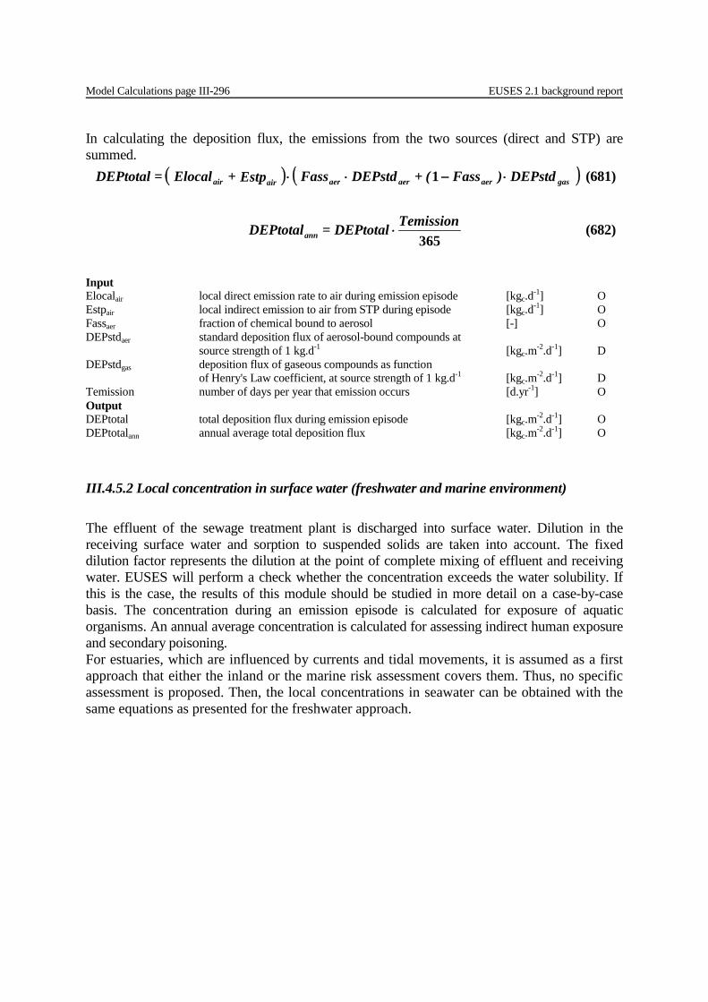
Model Calculations page III-296 EUSES 2.1 background report
In calculating the deposition flux, the emissions from the two sources (direct and STP) are summed.
Input Elocalair local direct emission rate to air during emission episode [kgc.d-1] O Estpair local indirect emission to air from STP during episode [kgc.d-1] O Fassaer fraction of chemical bound to aerosol [-] O DEPstdaer standard deposition flux of aerosol-bound compounds at source strength of 1 kg.d-1 [kgc.m-2.d-1] D DEPstdgas deposition flux of gaseous compounds as function of Henry's Law coefficient, at source strength of 1 kg.d-1 [kgc.m-2.d-1] D Temission number of days per year that emission occurs [d.yr-1] O Output DEPtotal total deposition flux during emission episode [kgc.m-2.d-1] O DEPtotalann annual average total deposition flux [kgc.m-2.d-1] O
III.4.5.2 Local concentration in surface water (freshwater and marine environment) The effluent of the sewage treatment plant is discharged into surface water. Dilution in the receiving surface water and sorption to suspended solids are taken into account. The fixed dilution factor represents the dilution at the point of complete mixing of effluent and receiving water. EUSES will perform a check whether the concentration exceeds the water solubility. If this is the case, the results of this module should be studied in more detail on a case-by-case basis. The concentration during an emission episode is calculated for exposure of aquatic organisms. An annual average concentration is calculated for assessing indirect human exposure and secondary poisoning. For estuaries, which are influenced by currents and tidal movements, it is assumed as a first approach that either the inland or the marine risk assessment covers them. Thus, no specific assessment is proposed. Then, the local concentrations in seawater can be obtained with the same equations as presented for the freshwater approach.
( ) ( ) DEPstd )Fass( + DEPstd Fass Estp + Elocal = DEPtotal gasaeraeraerairair ⋅−⋅⋅ 1 (681)
365
Temission DEPtotal= DEPtotalann ⋅ (682)
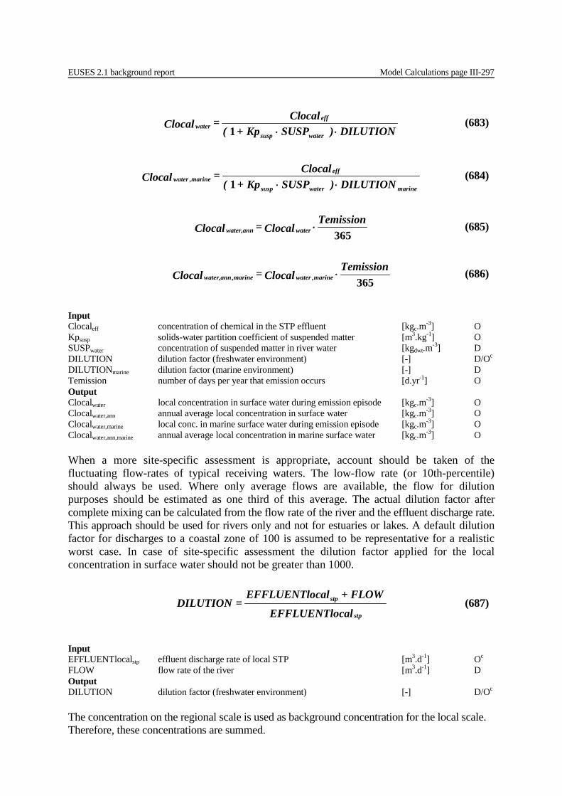
EUSES 2.1 background report Model Calculations page III-297
Input Clocaleff concentration of chemical in the STP effluent [kgc.m-3] O Kpsusp solids-water partition coefficient of suspended matter [m3.kg-1] O SUSPwater concentration of suspended matter in river water [kgdwt.m-3] D DILUTION dilution factor (freshwater environment) [-] D/Oc DILUTIONmarine dilution factor (marine environment) [-] D Temission number of days per year that emission occurs [d.yr-1] O Output Clocalwater local concentration in surface water during emission episode [kgc.m-3] O Clocalwater,ann annual average local concentration in surface water [kgc.m-3] O Clocalwater,marine local conc. in marine surface water during emission episode [kgc.m-3] O Clocalwater,ann,marine annual average local concentration in marine surface water [kgc.m-3] O When a more site-specific assessment is appropriate, account should be taken of the fluctuating flow-rates of typical receiving waters. The low-flow rate (or 10th-percentile) should always be used. Where only average flows are available, the flow for dilution purposes should be estimated as one third of this average. The actual dilution factor after complete mixing can be calculated from the flow rate of the river and the effluent discharge rate. This approach should be used for rivers only and not for estuaries or lakes. A default dilution factor for discharges to a coastal zone of 100 is assumed to be representative for a realistic worst case. In case of site-specific assessment the dilution factor applied for the local concentration in surface water should not be greater than 1000.
Input EFFLUENTlocalstp effluent discharge rate of local STP [m3.d-1] Oc FLOW flow rate of the river [m3.d-1] D Output DILUTION dilution factor (freshwater environment) [-] D/Oc The concentration on the regional scale is used as background concentration for the local scale. Therefore, these concentrations are summed.
DILUTION ) SUSP Kp + (
Clocal= Clocalwatersusp
effwater ⋅⋅1
(683)
marinewatersusp
effmarinewater DILUTION ) SUSP Kp + (
Clocal= Clocal⋅⋅1, (684)
365
Temission Clocal= Clocal waterannwater, ⋅ (685)
365,,
Temission Clocal= Clocal marinewatermarineannwater, ⋅ (686)
calEFFLUENTlo
FLOW+ calEFFLUENTlo= DILUTION
stp
stp (687)
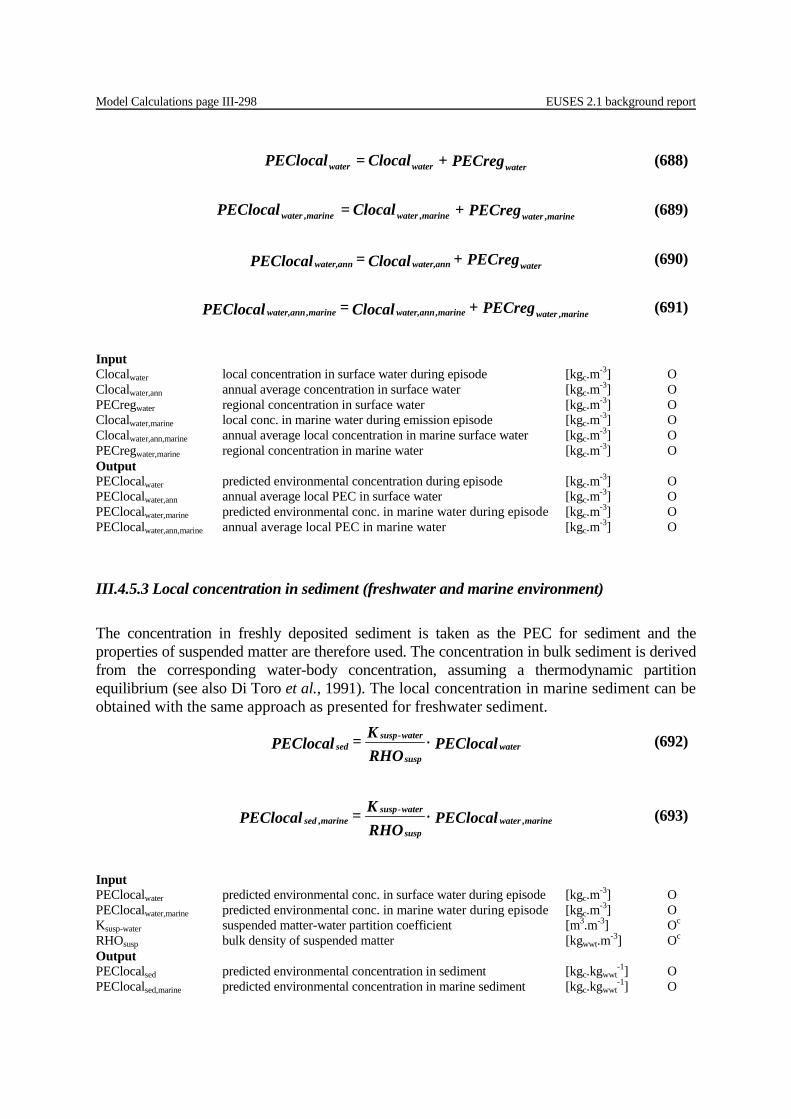
Model Calculations page III-298 EUSES 2.1 background report
Input Clocalwater local concentration in surface water during episode [kgc.m-3] O Clocalwater,ann annual average concentration in surface water [kgc.m-3] O PECregwater regional concentration in surface water [kgc.m-3] O Clocalwater,marine local conc. in marine water during emission episode [kgc.m-3] O Clocalwater,ann,marine annual average local concentration in marine surface water [kgc.m-3] O PECregwater,marine regional concentration in marine water [kgc.m-3] O Output PEClocalwater predicted environmental concentration during episode [kgc.m-3] O PEClocalwater,ann annual average local PEC in surface water [kgc.m-3] O PEClocalwater,marine predicted environmental conc. in marine water during episode [kgc.m-3] O PEClocalwater,ann,marine annual average local PEC in marine water [kgc.m-3] O
III.4.5.3 Local concentration in sediment (freshwater and marine environment) The concentration in freshly deposited sediment is taken as the PEC for sediment and the properties of suspended matter are therefore used. The concentration in bulk sediment is derived from the corresponding water-body concentration, assuming a thermodynamic partition equilibrium (see also Di Toro et al., 1991). The local concentration in marine sediment can be obtained with the same approach as presented for freshwater sediment.
Input PEClocalwater predicted environmental conc. in surface water during episode [kgc.m-3] O PEClocalwater,marine predicted environmental conc. in marine water during episode [kgc.m-3] O Ksusp-water suspended matter-water partition coefficient [m3.m-3] Oc RHOsusp bulk density of suspended matter [kgwwt.m-3] Oc Output PEClocalsed predicted environmental concentration in sediment [kgc.kgwwt
-1] O PEClocalsed,marine predicted environmental concentration in marine sediment [kgc.kgwwt
-1] O
PECreg + Clocal= PEClocal waterwaterwater (688)
PECreg + Clocal= PEClocal marinewatermarinewatermarinewater ,,, (689)
PECreg + Clocal= PEClocal waterannwater,annwater, (690)
PECreg + Clocal= PEClocal marinewatermarineannwater,marineannwater, ,,, (691)
PEClocal RHOK= PEClocal water
susp
water-suspsed ⋅ (692)
PEClocal RHOK= PEClocal marinewater
susp
water-suspmarinesed ,, ⋅ (693)
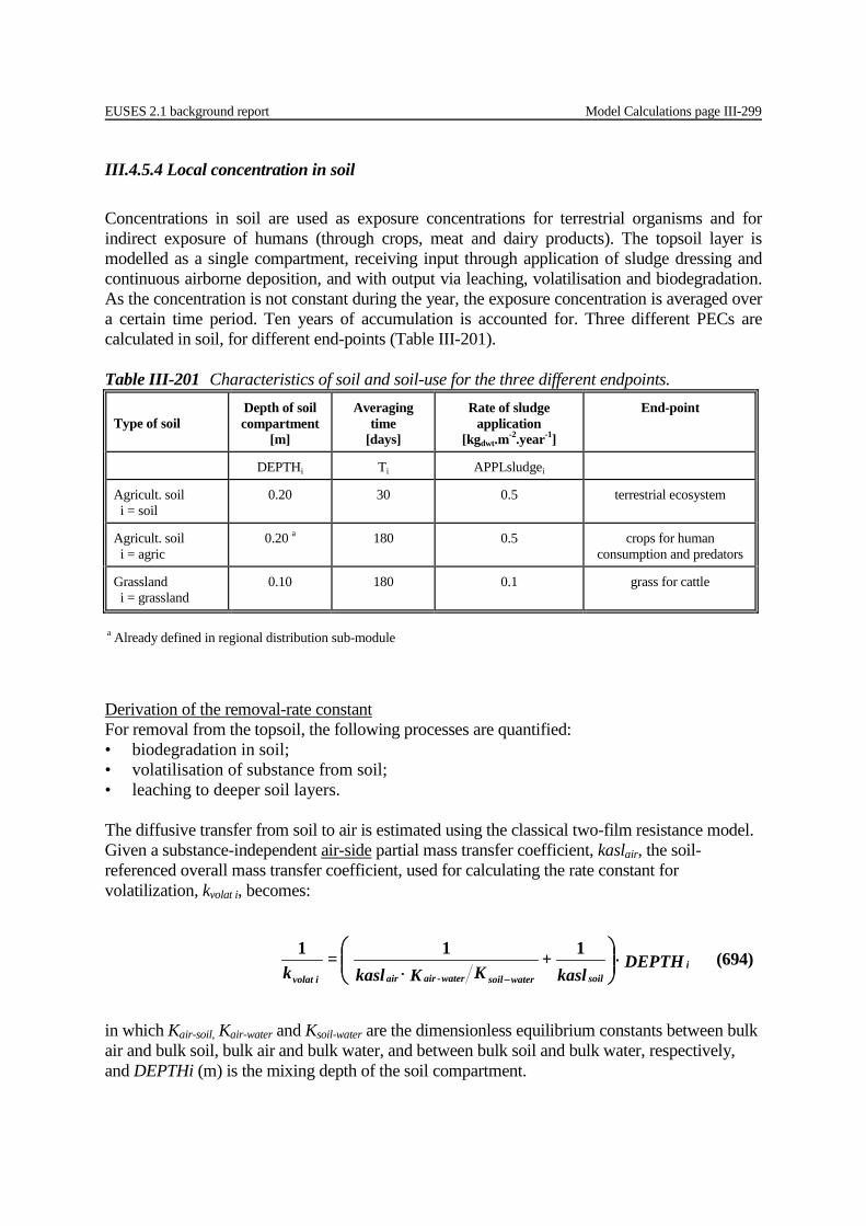
EUSES 2.1 background report Model Calculations page III-299
III.4.5.4 Local concentration in soil Concentrations in soil are used as exposure concentrations for terrestrial organisms and for indirect exposure of humans (through crops, meat and dairy products). The topsoil layer is modelled as a single compartment, receiving input through application of sludge dressing and continuous airborne deposition, and with output via leaching, volatilisation and biodegradation. As the concentration is not constant during the year, the exposure concentration is averaged over a certain time period. Ten years of accumulation is accounted for. Three different PECs are calculated in soil, for different end-points (Table III-201).
Derivation of the removal-rate constant For removal from the topsoil, the following processes are quantified: • biodegradation in soil; • volatilisation of substance from soil; • leaching to deeper soil layers. The diffusive transfer from soil to air is estimated using the classical two-film resistance model. Given a substance-independent air-side partial mass transfer coefficient, kaslair, the soil-referenced overall mass transfer coefficient, used for calculating the rate constant for volatilization, kvolat i, becomes:
in which Kair-soil, Kair-water and Ksoil-water are the dimensionless equilibrium constants between bulk air and bulk soil, bulk air and bulk water, and between bulk soil and bulk water, respectively, and DEPTHi (m) is the mixing depth of the soil compartment.
Table III-201 Characteristics of soil and soil-use for the three different endpoints. Type of soil
Depth of soil compartment
[m]
Averaging time
[days]
Rate of sludge application
[kgdwt.m-2.year-1]
End-point
DEPTHi Ti APPLsludgei
Agricult. soil i = soil
0.20 30 0.5 terrestrial ecosystem
Agricult. soil i = agric
0.20 a 180 0.5 crops for human consumption and predators
Grassland i = grassland
0.10 180 0.1 grass for cattle
a Already defined in regional distribution sub-module
DEPTH kasl
+ KK kasl
= k i
soilwatersoilwater-airairivolat
⋅
⋅ −
111 (694)
Model Calculations page III-300 EUSES 2.1 background report
Input kaslair partial mass-transfer coeff. at air side of air-soil interface [m.d-1] D kaslsoil partial mass-transfer coeff. at soil side of air-soil interface [m.d-1] O Kair-water air-water partition coefficient [m3.m-3] Oc Ksoil-water soil-water partition coefficient [m3.m-3] Oc DEPTHi mixing depth of soil type i [m] D Output kvolat i rate constant for volatilisation from soil i [d-1] O A first-order rate constant for leaching can be calculated from the amount of rain flushing the liquid phase of the soil compartment.
Input Finfsoil fraction of rainwater that infiltrates into soil [-] D RAINRATE rate of wet precipitation [m.d-1] D Ksoil-water soil-water partition coefficient [m3.m-3] Oc DEPTHi mixing depth of soil type i [m] D Output kleach i rate constant for leaching from soil i [d-1] O The overall removal-rate constant is given by the sum of all relevant-removal rate constants.
Input kvolat i rate constant for volatilisation from soil i [d-1] O kleach i rate constant for leaching from topsoil i [d-1] O kdegsoil rate constant for degradation in soil [d-1] O Output ki rate constant for removal from topsoil i [d-1] O
DEPTH K
RAINRATE Finf= kiwater-soil
soili leach ⋅
⋅ (695)
kdeg + k + k= k soili leachi volati (696)
EUSES 2.1 background report Model Calculations page III-301
Referencing deposition flux to kg soil To simplify the calculations, the airborne deposition flux (Section III.4.5.1) is referenced to kg substance per kg of soil per day. The total deposition flux is converted as follows:
Input DEPtotalann annual average total deposition flux [kgc.m-2.d-1] O DEPTHi mixing depth of soil type i [m] D RHOsoil bulk density of soil [kgwwt.m-3] Oc Output Dair i airborne deposition flux per kg of soil i [kgc.kgwwt
-1.d-1] Oc Initial concentration after 10 years of sludge application To take accumulation in soil into account, sludge application is assessed for 10 consecutive years. The PEC in soil is the concentration in the 10th year, averaged over a time period T. As a first step, the initial concentration in this year needs to be derived. The contributions of deposition and sludge applications are considered separately. The concentration due to 10 years of continuous deposition only is given by:
Input Dair i airborne deposition flux per kg of soil i [kgc.kgwwt
-1.d-1] O ki rate constant for removal from top-soil i [d-1] O Output Cdep10i concentration in soil i due to deposition in 10th year at t=0 [kgc.kgwwt
-1] Oc Sludge application is not a continuous process, but is assumed to take place once a year at the beginning of each year. The concentration just after the first year of sludge application is given by:
Input Csludge concentration in dry sewage sludge [kgc.kgdwt
-1] O APPLsludgei dry sludge application rate on soil i [kgdwt.m-2.yr-1] D DEPTHi mixing depth of soil type i [m] D RHOsoil bulk density of soil [kgwwt.m-3] Oc Output Csludge1i concentration in soil due to sludge in first year at t=0 [kgc.kgwwt
-1] Oc
RHO DEPTH
DEPtotal= Dsoili
anni air ⋅
(697)
e k
D -k
D= Cdep10 ik
i
i air
i
i airi
⋅⋅−⋅ 10365 (698)
soili
isludgei RHODEPTH
APPLsludgeC= Csludge1
⋅
⋅ (699)
Model Calculations page III-302 EUSES 2.1 background report
At the end of each year, a fraction Facc of the initial concentration remains in the topsoil layer. Using this fraction, the initial concentration after 10 applications of sludge can be assessed.
Input ki rate constant for removal from top soil i [d-1] O Facci fraction accumulating in one year in soil i [-] Oc Csludge1i concentration in soil i due to sludge in first year at t=0 [kgc.kgwwt
-1] Oc Output Csludge10i concentration in soil i due to sludge in 10th year at t=0 [kgc.kgwwt
-1] Oc The sum of the concentrations due to deposition and to sludge is the initial concentration in year 10.
Input Csludge10i concentration in soil i due to sludge in 10th year at t=0 [kgc.kgwwt
-1] Oc Cdep10i concentration in soil i due to deposition in 10th year at t=0 [kgc.kgwwt
-1] Oc Output Clocal10i initial concentration in soil i (in 10th year at t=0) [kgc.kgwwt
-1] Oc Local concentration in soil The fate of the chemical in soil is modelled with a one-compartment model with a continuous input from airborne deposition and continuous elimination from the topsoil layer. The initial condition is given by Clocal10i. The differential equation describing the one-compartment model can be solved analytically to give the concentration in soil as a function of time. The exposure concentration in soil was defined as the average concentration over a certain time period T, and is thus defined by the integral of the concentration in soil i from 0 to T days:
e= Facc ik-i
365 (700)
⋅ ∑ Facc + Csludge1= Csludge10 i
n
= nii
9
1
1 (701)
iii Csludge10 + Cdep10= Clocal10 (702)
dt (t) Clocal T
= Clocal i
T
ii
i
∫⋅0
1 (703)
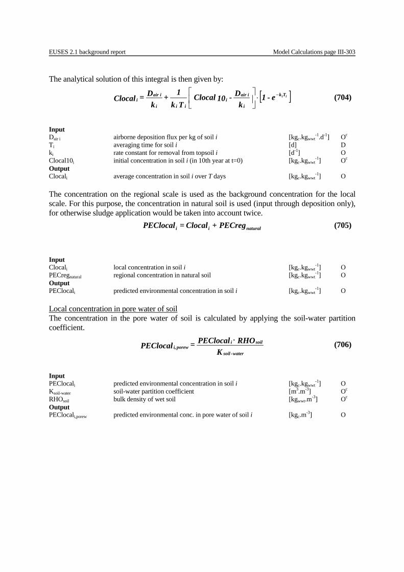
EUSES 2.1 background report Model Calculations page III-303
The analytical solution of this integral is then given by:
Input Dair i airborne deposition flux per kg of soil i [kgc.kgwwt
-1.d-1] Oc Ti averaging time for soil i [d] D ki rate constant for removal from topsoil i [d-1] O Clocal10i initial concentration in soil i (in 10th year at t=0) [kgc.kgwwt
-1] Oc Output Clocali average concentration in soil i over T days [kgc.kgwwt
-1] O The concentration on the regional scale is used as the background concentration for the local scale. For this purpose, the concentration in natural soil is used (input through deposition only), for otherwise sludge application would be taken into account twice.
Input Clocali local concentration in soil i [kgc.kgwwt
-1] O PECregnatural regional concentration in natural soil [kgc.kgwwt
-1] O Output PEClocali predicted environmental concentration in soil i [kgc.kgwwt
-1] O Local concentration in pore water of soil The concentration in the pore water of soil is calculated by applying the soil-water partition coefficient.
Input PEClocali predicted environmental concentration in soil i [kgc.kgwwt
-1] O Ksoil-water soil-water partition coefficient [m3.m-3] Oc RHOsoil bulk density of wet soil [kgwwt.m-3] Oc Output PEClocali,porew predicted environmental conc. in pore water of soil i [kgc.m-3] O
[ ]iiTk
i
i airi
iii
i airi e-1
kD -10Clocal
T k1 +
kD= Clocal −⋅
(704)
naturalii PECreg + Clocal= PEClocal (705)
K
RHO PEClocal= PEClocalwater-soil
soiliporewi,
⋅ (706)
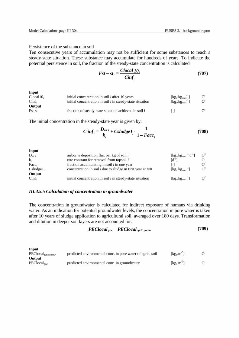
Model Calculations page III-304 EUSES 2.1 background report
Persistence of the substance in soil Ten consecutive years of accumulation may not be sufficient for some substances to reach a steady-state situation. These substance may accumulate for hundreds of years. To indicate the potential persistence in soil, the fraction of the steady-state concentration is calculated.
Input Clocal10i initial concentration in soil i after 10 years [kgc.kgwwt
-1] Oc Cinfi initial concentration in soil i in steady-state situation [kgc.kgwwt
-1] Oc Output Fst-sti fraction of steady-state situation achieved in soil i [-] Oc The initial concentration in the steady-state year is given by:
Input Dair i airborne deposition flux per kg of soil i [kgc.kgwwt
-1.d-1] Oc ki rate constant for removal from topsoil i [d-1] O Facci fraction accumulating in soil i in one year [-] Oc Csludge1i concentration in soil i due to sludge in first year at t=0 [kgc.kgwwt
-1] Oc Output Cinfi initial concentration in soil i in steady-state situation [kgc.kgwwt
-1] Oc
III.4.5.5 Calculation of concentration in groundwater The concentration in groundwater is calculated for indirect exposure of humans via drinking water. As an indication for potential groundwater levels, the concentration in pore water is taken after 10 years of sludge application to agricultural soil, averaged over 180 days. Transformation and dilution in deeper soil layers are not accounted for.
Input PEClocalagric,porew predicted environmental conc. in pore water of agric. soil [kgc.m-3] O Output PEClocalgrw predicted environmental conc. in groundwater [kgc.m-3] O
Cinf
10Clocal= stFsti
ii− (707)
i
ii
i airi Facc
Csludge1 + k
D= infC−
⋅1
1 (708)
PEClocal= PEClocal porewagric,grw (709)
EUSES 2.1 background report Model Calculations page III-305
III.5 EXPOSURE MODULE In the exposure module, exposure levels for humans and predating birds and mammals are estimated. This module is divided into four specific sub-modules, which will be handled separately: • Secondary poisoning. • Indirect human exposure. • Consumer exposure. • Workplace exposure. III.5.1 Secondary poisoning For the assessment of secondary poisoning, three example food chains are modelled: 1. water (freshwater and marine environment)→fish→predator 2. water (marine environment)→fish→predator→toppredator 3. soil→worm→predator. Exposure levels are calculated, assuming a scenario whereby 50% of the food is sourced from the local environment and 50% from the regional environment. Input: chemical properties Kow octanol-water partition coefficient [-] Input: environmental properties RHOsoil bulk density of soil [kgwwt.m-3] c CONVsoil conversion factor for soil concentrations: wwt to dwt [kgwwt.kgdwt
-1] c
PEClocalwater,ann annual average local PEC in surface water (dissolved) [kgc.m-3] PEClocalwater,ann,marine annual average local PEC in marine surface water (dissolved) [kgc.m-3] PEClocalagric local PEC in agricultural soil [kgc. kgwwt
-1] PEClocalagric,porew local PEC in pore water of agricultural soil [kgc.m-3] PECregwater regional PEC in surface water (dissolved) [kgc.m-3] PECregwater,marine regional PEC in marine surface water (dissolved) [kgc.m-3] PECregagric regional PEC in agricultural soil [kgc.kgwwt
-1] PECregagric,porew regional PEC in pore water of agricultural soil [kgc.m-3] Intermediate results BCFworm bioconcentration factor for earthworms [kgsoil wwt.kgworm wwt
-1] BCFfish bioconcentration factor for fish [m3.kgwwt
-1] Output BCFfish bioconcentration factor for fish [m3.kgwwt
-1] PECoral,fish concentration in fish from surface water for predators [kgc.kgwwt
-1] PECoral,fish,marine concentration in fish from marine surface water for predators [kgc.kgwwt
-1] PECoral,fish predator,marine concentration in fish-eating predator for marine toppredators [kgc.kgwwt
-1] PECoral,worm concentration in earthworms from agricultural soil [kgc.kgwwt
-1]
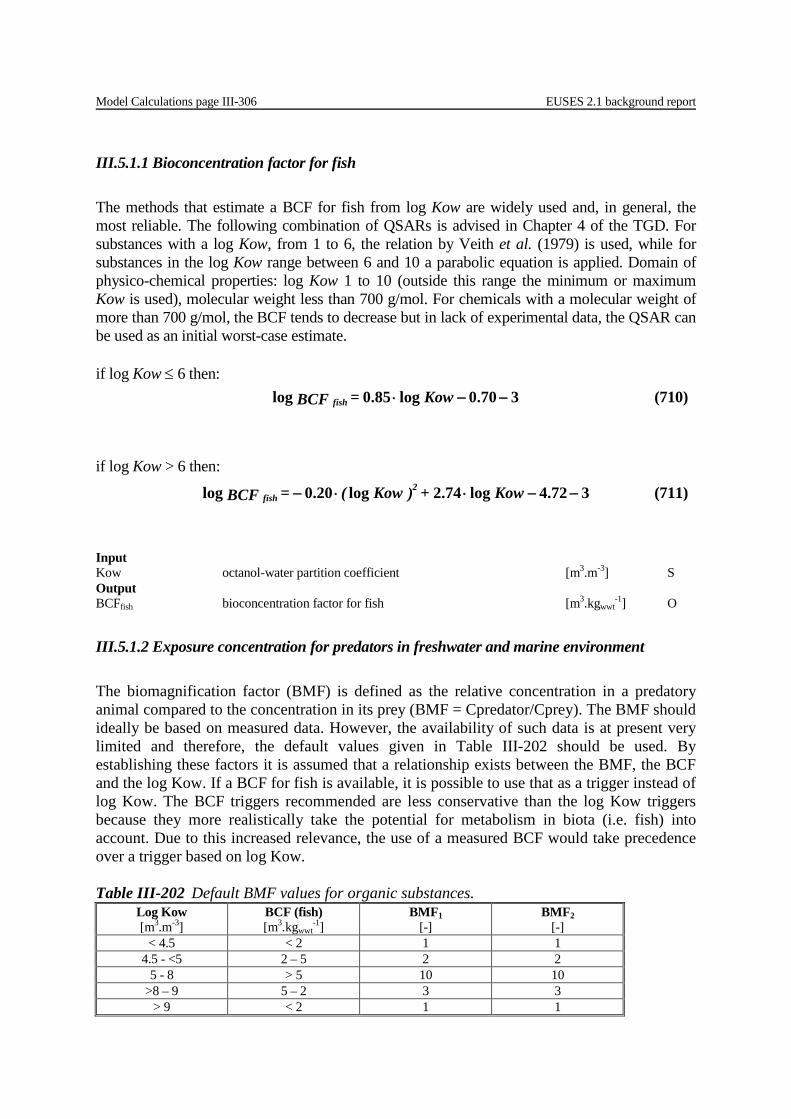
Model Calculations page III-306 EUSES 2.1 background report
III.5.1.1 Bioconcentration factor for fish The methods that estimate a BCF for fish from log Kow are widely used and, in general, the most reliable. The following combination of QSARs is advised in Chapter 4 of the TGD. For substances with a log Kow, from 1 to 6, the relation by Veith et al. (1979) is used, while for substances in the log Kow range between 6 and 10 a parabolic equation is applied. Domain of physico-chemical properties: log Kow 1 to 10 (outside this range the minimum or maximum Kow is used), molecular weight less than 700 g/mol. For chemicals with a molecular weight of more than 700 g/mol, the BCF tends to decrease but in lack of experimental data, the QSAR can be used as an initial worst-case estimate. if log Kow ≤ 6 then:
if log Kow > 6 then:
Input Kow octanol-water partition coefficient [m3.m-3] S Output BCFfish bioconcentration factor for fish [m3.kgwwt
-1] O
III.5.1.2 Exposure concentration for predators in freshwater and marine environment The biomagnification factor (BMF) is defined as the relative concentration in a predatory animal compared to the concentration in its prey (BMF = Cpredator/Cprey). The BMF should ideally be based on measured data. However, the availability of such data is at present very limited and therefore, the default values given in Table III-202 should be used. By establishing these factors it is assumed that a relationship exists between the BMF, the BCF and the log Kow. If a BCF for fish is available, it is possible to use that as a trigger instead of log Kow. The BCF triggers recommended are less conservative than the log Kow triggers because they more realistically take the potential for metabolism in biota (i.e. fish) into account. Due to this increased relevance, the use of a measured BCF would take precedence over a trigger based on log Kow. Table III-202 Default BMF values for organic substances.
Log Kow [m3.m-3]
BCF (fish) [m3.kgwwt
-1] BMF1
[-] BMF2
[-] < 4.5 < 2 1 1
4.5 - <5 2 – 5 2 2 5 - 8 > 5 10 10
>8 – 9 5 – 2 3 3 > 9 < 2 1 1
370.0log85.0log −−⋅ Kow = BCF fish (710)
372.4log74.2log20.0log −−⋅⋅− Kow + )Kow ( = BCF 2fish (711)
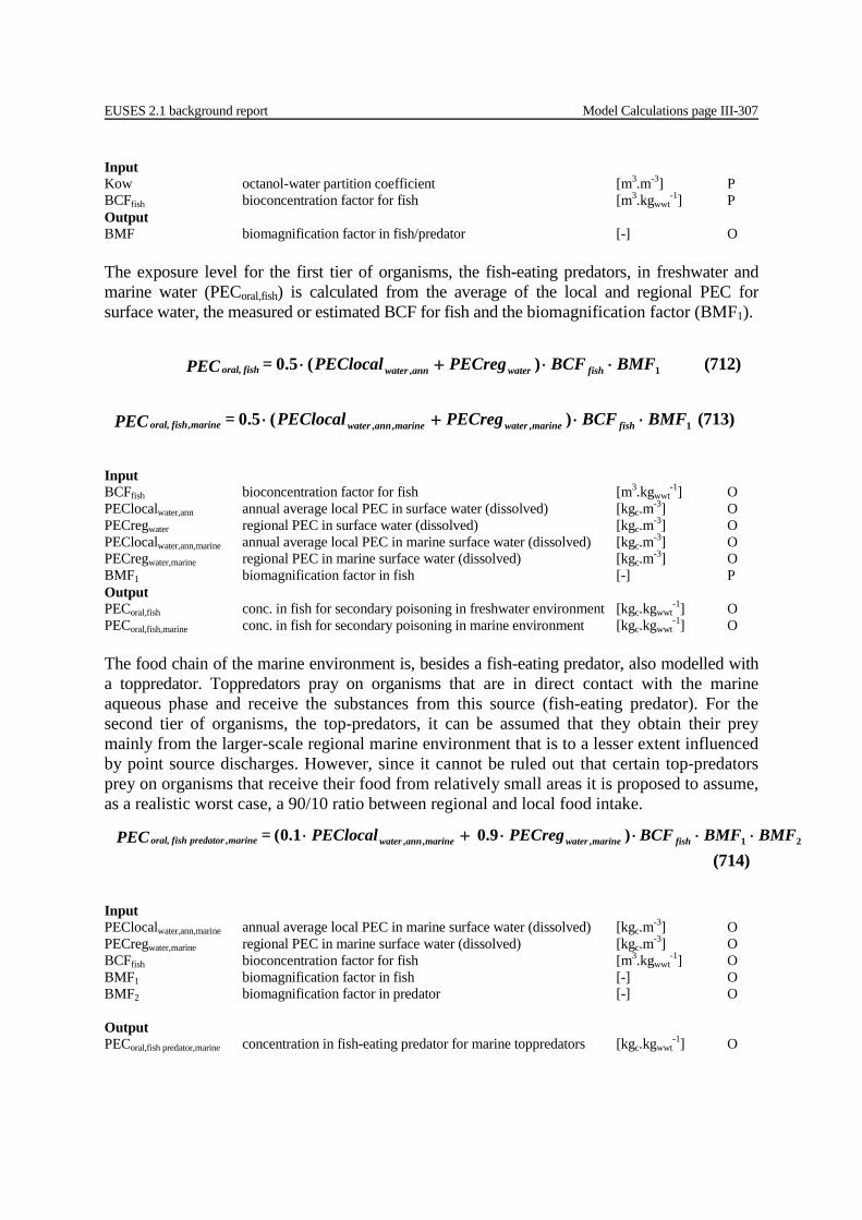
EUSES 2.1 background report Model Calculations page III-307
Input Kow octanol-water partition coefficient [m3.m-3] P BCFfish bioconcentration factor for fish [m3.kgwwt
-1] P Output BMF biomagnification factor in fish/predator [-] O The exposure level for the first tier of organisms, the fish-eating predators, in freshwater and marine water (PECoral,fish) is calculated from the average of the local and regional PEC for surface water, the measured or estimated BCF for fish and the biomagnification factor (BMF1).
Input BCFfish bioconcentration factor for fish [m3.kgwwt
-1] O PEClocalwater,ann annual average local PEC in surface water (dissolved) [kgc.m-3] O PECregwater regional PEC in surface water (dissolved) [kgc.m-3] O PEClocalwater,ann,marine annual average local PEC in marine surface water (dissolved) [kgc.m-3] O PECregwater,marine regional PEC in marine surface water (dissolved) [kgc.m-3] O BMF1 biomagnification factor in fish [-] P Output PECoral,fish conc. in fish for secondary poisoning in freshwater environment [kgc.kgwwt
-1] O PECoral,fish,marine conc. in fish for secondary poisoning in marine environment [kgc.kgwwt
-1] O The food chain of the marine environment is, besides a fish-eating predator, also modelled with a toppredator. Toppredators pray on organisms that are in direct contact with the marine aqueous phase and receive the substances from this source (fish-eating predator). For the second tier of organisms, the top-predators, it can be assumed that they obtain their prey mainly from the larger-scale regional marine environment that is to a lesser extent influenced by point source discharges. However, since it cannot be ruled out that certain top-predators prey on organisms that receive their food from relatively small areas it is proposed to assume, as a realistic worst case, a 90/10 ratio between regional and local food intake.
Input PEClocalwater,ann,marine annual average local PEC in marine surface water (dissolved) [kgc.m-3] O PECregwater,marine regional PEC in marine surface water (dissolved) [kgc.m-3] O BCFfish bioconcentration factor for fish [m3.kgwwt
-1] O BMF1 biomagnification factor in fish [-] O BMF2 biomagnification factor in predator [-] O Output PECoral,fish predator,marine concentration in fish-eating predator for marine toppredators [kgc.kgwwt
-1] O
1, )(5.0 BMFBCFPECregPEClocal= PEC fishwaterannwaterfishoral, ⋅⋅+⋅ (712)
1,,,, )(5.0 BMFBCFPECregPEClocal= PEC fishmarinewatermarineannwatermarinefishoral, ⋅⋅+⋅ (713)
21,,,, )9.01.0( BMFBMFBCFPECreg PEClocal= PEC fishmarinewatermarineannwatermarinepredatorfishoral, ⋅⋅⋅⋅+⋅
(714)

Model Calculations page III-308 EUSES 2.1 background report
III.5.1.3 Bioconcentration factor for earthworms For organic chemicals, the main route of uptake into earthworms will be via the interstitial water. Bioconcentration can be described as a hydrophobic partitioning between the pore water and the phases inside the organism and is modelled according to the equation as described by Jager (1998). The model was supported by data with neutral organic chemicals in soil within the range log Kow 3-8 and in water-only experiments from log Kow 1-6. An application range of log Kow 1-8 is advised and it is reasonable to assume that extrapolation to lower Kow values is possible. Table III-203 Default settings for earthworm specific parameters.
Parameter Symbol Unit Value
Fraction of water inside the worm (volume fraction) Fwaterworm [-] 0.84
Fraction of lipids inside the worm (volume fraction) Flipidworm [-] 0.012
Density of earthworms RHOworm [kgwwt.m-3] 1000
Fraction of gut loading in worm Fgutworm [kgdwt.kgwwt-1] 0.1
worm
wormwormworm RHO
KowFlipidFwater= BCF
⋅+ (715)
Input Fwaterworm fraction of water inside the worm (volume fraction) [-] D Flipidworm fraction of lipids inside the worm (volume fraction) [-] D Kow octanol-water partition coefficient [m3.m-3] S RHOworm density of earthworms [kgwwt.m-3] D Output BCFworm bioconcentration factor for earthworms [m3.kgwwt
-1] O
III.5.1.4 Exposure concentration for worm-eating predators The concentration in earthworms for secondary poisoning is estimated from the BCF, the gut loading of earthworms and the average of regional and local concentrations in agricultural soil and porewater. The gut loading of earthworms depends heavily on soil conditions and available food. Reported values range from 2-20 % (kgdwt gut/kgwwt voided worm), 10% can therefore be taken as a reasonable value.
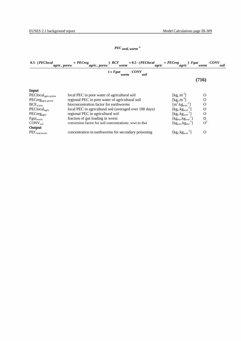
EUSES 2.1 background report Model Calculations page III-309
soilCONV
wormFgut
soilCONV
wormFgut
agricPECreg
agricPEClocal
wormBCF
porewagricPECreg
porewagricPEClocal
= PEC wormoral,
⋅+
⋅⋅+⋅+⋅+⋅
1
)(5.0),,
(5.0
(716) Input PEClocalagric,porew local PEC in pore water of agricultural soil [kgc.m-3] O PECregagric,porew regional PEC in pore water of agricultural soil [kgc.m-3] O BCFworm bioconcentration factor for earthworms [m3.kgwwt
-1] O PEClocalagric local PEC in agricultural soil (averaged over 180 days) [kgc.kgwwt
-1] O PECregagric regional PEC in agricultural soil [kgc.kgwwt
-1] O Fgutworm fraction of gut loading in worm [kgdwt.kgwwt
-1] D CONVsoil conversion factor for soil concentrations: wwt to dwt [kgwwt.kgdwt
-1] OC
Output PECoral,worm concentration in earthworms for secondary poisoning [kgc.kgwwt
-1] O
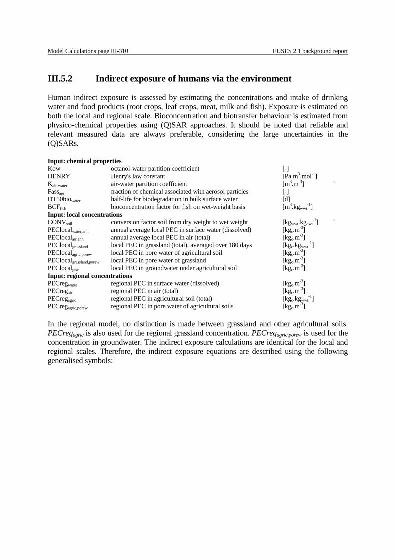
Model Calculations page III-310 EUSES 2.1 background report
III.5.2 Indirect exposure of humans via the environment Human indirect exposure is assessed by estimating the concentrations and intake of drinking water and food products (root crops, leaf crops, meat, milk and fish). Exposure is estimated on both the local and regional scale. Bioconcentration and biotransfer behaviour is estimated from physico-chemical properties using (Q)SAR approaches. It should be noted that reliable and relevant measured data are always preferable, considering the large uncertainties in the (Q)SARs. Input: chemical properties Kow octanol-water partition coefficient [-] HENRY Henry's law constant [Pa.m3.mol-1] Kair-water air-water partition coefficient [m3.m-3] c Fassaer fraction of chemical associated with aerosol particles [-] DT50biowater half-life for biodegradation in bulk surface water [d] BCFfish bioconcentration factor for fish on wet-weight basis [m3.kgwwt
-1] Input: local concentrations CONVsoil conversion factor soil from dry weight to wet weight [kgwwt.kgdwt
-1] c PEClocalwater,ann annual average local PEC in surface water (dissolved) [kgc.m-3] PEClocalair,ann annual average local PEC in air (total) [kgc.m-3] PEClocalgrassland local PEC in grassland (total), averaged over 180 days [kgc.kgwwt
-1] PEClocalagric,porew local PEC in pore water of agricultural soil [kgc.m-3] PEClocalgrassland,porew local PEC in pore water of grassland [kgc.m-3] PEClocalgrw local PEC in groundwater under agricultural soil [kgc.m-3] Input: regional concentrations PECregwater regional PEC in surface water (dissolved) [kgc.m-3] PECregair regional PEC in air (total) [kgc.m-3] PECregagric regional PEC in agricultural soil (total) [kgc.kgwwt
-1] PECregagric,porew regional PEC in pore water of agricultural soils [kgc.m-3] In the regional model, no distinction is made between grassland and other agricultural soils. PECregagric is also used for the regional grassland concentration. PECregagric,porew is used for the concentration in groundwater. The indirect exposure calculations are identical for the local and regional scales. Therefore, the indirect exposure equations are described using the following generalised symbols:
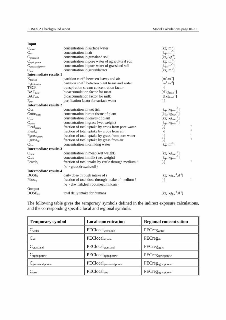
EUSES 2.1 background report Model Calculations page III-311
Input Cwater concentration in surface water [kgc.m-3] Cair concentration in air [kgc.m-3] Cgrassland concentration in grassland soil [kgc.kg-1] Cagric,porew concentration in pore water of agricultural soil [kgc.m-3] Cgrassland,porew concentration in pore water of grassland soil [kgc.m-3] Cgrw concentration in groundwater [kgc.m-3] Intermediate results 1 Kleaf-air partition coeff. between leaves and air [m3.m-3] Kplant-water partition coeff. between plant tissue and water [m3.m-3] TSCF transpiration stream concentration factor [-] BAFmeat bioaccumulation factor for meat [d.kgfood
-1] BAFmilk bioaccumulation factor for milk [d.kgfood
-1] Fpur purification factor for surface water [-] Intermediate results 2 Cfish concentration in wet fish [kgc.kgwwt
-1] Crootplant concentration in root tissue of plant [kgc.kgwwt
-1] Cleaf concentration in leaves of plant [kgc.kgwwt
-1] Cgrass concentration in grass (wet weight) [kgc.kgwwt
-1] Fleafporew fraction of total uptake by crops from pore water [-] c Fleafair fraction of total uptake by crops from air [-] c Fgrassporew fraction of total uptake by grass from pore water [-] c Fgrassair fraction of total uptake by grass from air [-] c Cdrw concentration in drinking water [kgc.m-3] Intermediate results 3 Cmeat concentration in meat (wet weight) [kgc.kgwwt
-1] Cmilk concentration in milk (wet weight) [kgc.kgwwt
-1] Fcattlei fraction of total intake by cattle through medium i [-] c i ∈ {grass,drw,air,soil} Intermediate results 4 DOSEi daily dose through intake of i [kgc.kgbw
-1.d-1] Fdosei fraction of total dose through intake of medium i [-] c i ∈ {drw,fish,leaf,root,meat,milk,air} Output DOSEtot total daily intake for humans [kgc.kgbw
-1.d-1] The following table gives the 'temporary' symbols defined in the indirect exposure calculations, and the corresponding specific local and regional symbols.
Temporary symbol Local concentration Regional concentration
Cwater PEClocalwater,ann PECregwater
Cair PEClocalair,ann PECregair
Cgrassland PEClocalgrassland PECregagric
Cagric,porew PEClocalagric,porew PECregagric,porew
Cgrassland,porew PEClocalgrassland,porew PECregagric,porew
Cgrw PEClocalgrw PECregagric,porew

Model Calculations page III-312 EUSES 2.1 background report
Temporary symbol Local concentration Regional concentration
Cfish Clocalfish Cregfish
Cleaf Clocalleaf Cregleaf
Cgrass Clocalgrass Creggrass
Fleafporew Flocal-leafporew Freg-leafporew
Fleafair Flocal-leafair Freg-leafair
Fgrassporew Flocal-grassporew Freg-grassporew
Fgrassair Flocal-grassair Freg-grassair
Croot Clocalroot Cregroot
Cmeat Clocalmeat Cregmeat
Cmilk Clocalmilk Cregmilk
Cdrw Clocaldrw Cregdrw
DOSEi DOSElocali DOSEregi
Fdosei Fdose-locali Fdose-regi
DOSEtot DOSElocaltot DOSEregtot
III.5.2.1 Concentration in fish The BCF for fish is estimated in Section III.5.1.1 on secondary poisoning. The concentration in fish for human indirect exposure is given by:
Input BCFfish bioconcentration factor for fish on wet-weight basis [m3.kgwwt
-1] O Cwater concentration in surface water [kgc.m-3] O Output Cfish concentration in wet fish [kgc.kgwwt
-1] O
III.5.2.2 Concentration in crops The modelling approach proposed by Trapp and Matthies (1995) is used to estimate levels in plants due to uptake from pore water and air (gas phase). This approach integrates uptake from
C BCF= C waterfishfish ⋅ (717)
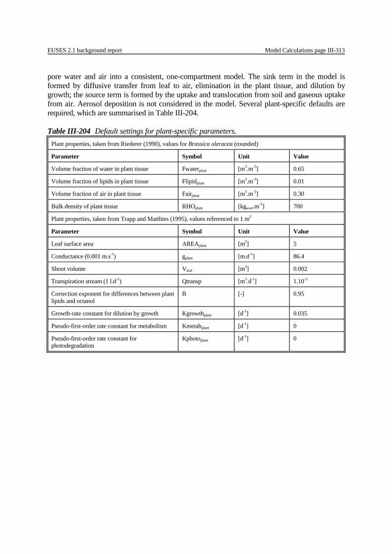
EUSES 2.1 background report Model Calculations page III-313
pore water and air into a consistent, one-compartment model. The sink term in the model is formed by diffusive transfer from leaf to air, elimination in the plant tissue, and dilution by growth; the source term is formed by the uptake and translocation from soil and gaseous uptake from air. Aerosol deposition is not considered in the model. Several plant-specific defaults are required, which are summarised in Table III-204.
Table III-204 Default settings for plant-specific parameters. Plant properties, taken from Riederer (1990), values for Brassica oleracea (rounded)
Parameter Symbol Unit Value
Volume fraction of water in plant tissue Fwaterplant [m3.m-3] 0.65
Volume fraction of lipids in plant tissue Flipidplant [m3.m-3] 0.01
Volume fraction of air in plant tissue Fairplant [m3.m-3] 0.30
Bulk density of plant tissue RHOplant [kgwwt.m-3] 700
Plant properties, taken from Trapp and Matthies (1995), values referenced to 1 m2
Parameter Symbol Unit Value
Leaf surface area AREAplant [m2] 5
Conductance (0.001 m.s-1) gplant [m.d-1] 86.4
Shoot volume Vleaf [m3] 0.002
Transpiration stream (1 l.d-1) Qtransp [m3.d-1] 1.10-3
Correction exponent for differences between plant lipids and octanol
B [-] 0.95
Growth-rate constant for dilution by growth Kgrowthplant [d-1] 0.035
Pseudo-first-order rate constant for metabolism Kmetabplant [d-1] 0
Pseudo-first-order rate constant for photodegradation
Kphotoplant [d-1] 0
Model Calculations page III-314 EUSES 2.1 background report
The general partitioning between water and plant tissue is assumed to be based on hydrophobic sorption to plant lipids. Kow is corrected slightly for the differences between plant lipids and octanol.
Input Fwaterplant volume fraction of water in plant tissue [m3.m-3] D Flipidplant volume fraction of lipids in plant tissue [m3.m-3] D Kow octanol-water partition coefficient [m3.m-3] S b correction for differences between plant lipids and octanol [-] D Output Kplant-water partition coeff. between plant tissue and water [m3.m-3] O The concentration in root tissue is governed mainly by physical sorption, and is given by:
Input Kplant-water partition coeff. between plant tissue and water [m3.m-3] O Cagric,porew concentration in pore water of agricultural soil [kgc.m-3] O RHOplant bulk density of plant tissue (wet weight) [kgwwt.m-3] D Output Croot concentration in root tissue of plant [kgc.kgwwt
-1] O The transpiration-stream concentration factor (TSCF) is the ratio between the concentration in the transpiration stream and the concentration in pore water. TSCF is given by (Briggs et al., 1982). This estimation of TSCF was derived for a small group of pesticides in one plant species (Barley). Domain of physico-chemical properties: log Kow -0.5 to 4.5 (outside this range the minimum or maximum Kow is used).
Input Kow octanol-water partition coefficient [-] S Output TSCF transpiration-stream concentration factor [-] O
Kow Flipid+ = Fwater K bplantplantwaterplant ⋅− (718)
RHO
C K= Cplant
porewagric,water-plantroot
⋅ (719)
⋅
44.278.1logexp784.0
2) Kow - ( - = TSCF (720)
EUSES 2.1 background report Model Calculations page III-315
Gaseous exchange between leaves and air can be described by a leaf-air partition coefficient. Kleaf-air is given by:
Input Kplant-water partition coefficient between plant tissue and water [m3.m-3] O Kair-water air-water partition coefficient [m3.m-3] Oc Fairplant volume fraction of air in plant tissue [m3.m-3] D Output Kleaf-air partition coeff. between leaves and air [m3.m-3] O Elimination of the substance may take place in the leaf tissue by metabolism or photolysis. If rate constants are known for these processes, they may be added:
Input kmetabplant rate constant for metabolism in plants [d-1] D kphotoplant rate constant for photolysis in plants [d-1] D Output kelimplant rate constant for total elimination in plants [d-1] Oc The actual one-compartment model for calculating the concentration in the leaf can be described with a simple differential equation. The sink term is formed by diffusive transfer from leaf to air, elimination in the plant tissue and dilution by growth:
Input AREAplant leaf surface area [m2] D gplant conductance [m.d-1] D Kleaf-air partition coeff. between leaves and air [-] O Vleaf shoot volume [m3] D kelimplant rate constant for elimination in plants [d-1] Oc kgrowthplant rate constant for dilution by growth [d-1] D Output ALPHA sink term of differential equation [d-1] Oc
K
K + Fair= Kwater-air
water-plantplantair-leaf (721)
plantplantplant kphoto + kmetab= kelim (722)
plantplantleafair-leaf
plantplant kgrowthkelim+ V K
g AREA= ALPHA +
⋅
⋅ (723)

Model Calculations page III-316 EUSES 2.1 background report
The source term is formed by the uptake and translocation from soil and gaseous uptake from air. Since we have two pore-water concentrations, for agricultural soil and grassland, two separate source terms must be estimated. At the moment, the same default plant characteristics are used for grass as for crops.
Input Qtransp transpiration stream [m3.d-1] D Cagric,porew concentration in pore water of agricultural soil [kgc.m-3] O Cgrassland,porew concentration in pore water of grassland [kgc.m-3] O Cair concentration in air [kgc.m-3] O gplant leaf conductance [m.d-1] D TSCF transpiration-stream concentration factor [-] O Vleaf shoot volume [m3] D Fassaer fraction of substance adsorbed to aerosol [-] O Output BETAagric source term of differential equation for crops [kgc.m-3.d-1] Oc BETAgrass source term of differential equation for grass [kgc.m-3.d-1] Oc The steady-state concentration is calculated as the source term divided by the sink term. The default growth-dilution rate constant ensures that a steady state will always be reached within the relevant period of time (assuming constant exposure levels).
Input ALPHA sink term of differential equation [d-1] Oc BETAagric source term of differential equation, agricultural soil [kgc.m-3.d-1] Oc BETAgrass source term of differential equation, grassland [kgc.m-3.d-1] Oc RHOplant bulk density of plant tissue (wet weight) [kgwwt.m-3] D Output Cleaf concentration in leaves of plant [kgc.kgwwt
-1] O Cgrass concentration in grass [kgc.kgwwt
-1] O
V
AREA g C )Fass( + V
Qtransp TSCF C= BETAleaf
plantplantairaer
leafporewagricagric ⋅⋅⋅−⋅⋅ 1, (724)
VAREA g C )Fass(
+ V
Qtransp TSCF C= BETA
leaf
plantplantairaer
leafporewgrassland,grass
⋅⋅⋅−
⋅⋅
1
(725)
RHO
1 ALPHA
BETA= Cplant
agricleaf ⋅ (726)
RHO
1 ALPHA
BETA= Cplant
grassgrass ⋅ (727)
EUSES 2.1 background report Model Calculations page III-317
As additional information, the contribution of uptake from pore water and air to the total uptake is calculated.
Input Qtransp transpiration stream [m3.d-1] D Cagric,porew concentration in pore water of agricultural soil [kgc.m-3] O Cgrassland,porew concentration in pore water of grassland [kgc.m-3] O Cair concentration in air [kgc.m-3] O TSCF transpiration-stream concentration factor [-] O Vleaf shoot volume [m3] D Fassaer fraction of substance adsorbed to aerosol [-] O BETAagric source term of differential equation for crops [kgc.m-3.d-1] Oc BETAgrass source term of differential equation for grass [kgc.m-3.d-1] Oc Output Fleafporew fraction of total uptake by crops from pore water [-] Oc Fleafair fraction of total uptake by crops from air [-] Oc Fgrassporew fraction of total uptake by grass from pore water [-] Oc Fgrassair fraction of total uptake by grass from air [-] Oc
III.5.2.3 Concentration in meat and milk products Travis and Arms (1988) performed a log-linear regression analysis on experimentally derived bioaccumulation factors and the octanol-water partition coefficient. It should be noted that the uncertainty in these estimates is considerable. The concentrations in meat and milk are calculated by applying the bioaccumulation factors and summing the contributions from air, soil, grass and drinking water. The BAF for meat is derived from data on 36 organic compounds, with a log Kow range of 1.5 - 6.5. The BAF for milk was derived from data on 28 organic compounds, with a log Kow range of 3 - 6.5. Outside these ranges, the minimum or maximum Kow is used.
BETA
VQtransp TSCFC
= Fleafagric
leafporewagric,
porew
⋅⋅ (728)
BETA
VAREA g C )Fass-(
= Fleafagric
leaf
plantplantairaer
air
⋅⋅⋅1 (729)
BETA
VQtransp TSCF C
= Fgrassgrass
leafporewgrassland,
porew
⋅⋅ (730)
BETA
VAREA g C )Fass-(
= Fgrassgrass
leaf
plantplantairaer
air
⋅⋅⋅1 (731)
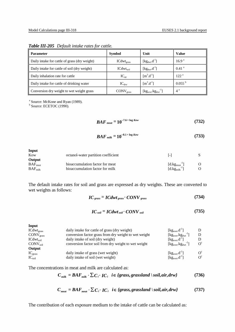
Model Calculations page III-318 EUSES 2.1 background report
Input Kow octanol-water partition coefficient [-] S Output BAFmeat bioaccumulation factor for meat [d.kgmeat
-1] O BAFmilk bioaccumulation factor for milk [d.kgmilk
-1] O The default intake rates for soil and grass are expressed as dry weights. These are converted to wet weights as follows:
Input ICdwtgrass daily intake for cattle of grass (dry weight) [kgwwt.d-1] D CONVgrass conversion factor grass from dry weight to wet weight [kgwwt.kgdwt
-1] D ICdwtsoil daily intake of soil (dry weight) [kgwwt.d-1] D CONVsoil conversion factor soil from dry weight to wet weight [kgwwt.kgdwt
-1] Oc Output ICgrass daily intake of grass (wet weight) [kgwwt.d-1] Oc ICsoil daily intake of soil (wet weight) [kgwwt.d-1] Oc The concentrations in meat and milk are calculated as:
The contribution of each exposure medium to the intake of cattle can be calculated as:
Table III-205 Default intake rates for cattle. Parameter Symbol Unit Value
Daily intake for cattle of grass (dry weight) ICdwtgrass [kgdwt.d-1] 16.9 a
Daily intake for cattle of soil (dry weight) ICdwtsoil [kgdwt.d-1] 0.41 a
Daily inhalation rate for cattle ICair [m3.d-1] 122 a
Daily intake for cattle of drinking water ICdrw [m3.d-1] 0.055 b
Conversion dry weight to wet weight grass CONVgrass [kgwwt.kgdwt-1] 4 a
a Source: McKone and Ryan (1989). b Source: ECETOC (1990).
10 log6.7 Kow + meat = BAF − (732)
10 log1.8 Kow + milk = BAF − (733)
CONV ICdwt= IC grassgrassgrass ⋅ (734)
CONV ICdwt= IC soilsoilsoil ⋅ (735)
drw}air,soil,\grassland{grass, i IC C BAF= C iimilkmilk ∈⋅∑⋅ (736)
drw}air,soil,\grassland{grass, i IC C BAF= C iimeatmeat ∈⋅∑⋅ (737)
EUSES 2.1 background report Model Calculations page III-319
Input Cgrass concentration in grass (wet weight) [kgc.kgwwt
-1] O ICgrass daily intake of grass (wet weight) [kgwwt.d-1] Oc Cgrassland total concentration in grassland soil (wet weight) [kgc.kgwwt
-1] O ICsoil daily intake of soil (wet weight) [kgwwt.d-1] Oc Cair total concentration in air [kgc.mair
-3] O ICair daily inhalation rate of cattle [mair
3.d-1] D Cdrw concentration in drinking water [kgc.mdrw
-3] O ICdrw daily intake of drinking water [mdrw
3.d-1] D Output Cmeat concentration in meat (wet weight) [kgc.kgwwt
-1] O Cmilk concentration in milk (wet weight) [kgc.kgwwt
-1] O Fcattlei fraction of total intake by cattle through i [-] Oc i ∈ {grass,soil,air,drw}
III.5.2.4 Concentration in drinking water Drinking water is produced from surface water or groundwater. Complete removal of suspended particles from surface water and groundwater is assumed. The effects of the treatment processes used for purification of groundwater, which are generally not intended for the removal of organic pollutants, can be neglected. Surface-water treatment is estimated according to Hrubec and Toet (1992). For the purification of river water for drinking water, a combination of extended storage of river water and extensive treatment is used. The storage is realised in open reservoirs and by means of artificial water recharge in the dunes. Dependent on the type of storage, two different water-treatment systems for surface water can be distinguished: • System 1:
- Storage in open reservoirs (volatilisation); - Coagulation, flocculation and rapid sand filtration; - Active carbon filtration.
• System 2: - Coagulation, flocculation and rapid sand filtration; - Dune water recharge; - Slow sand filtration.
The removal by ozonation of system 1 is not considered, because of the high uncertainty in the removal efficiency of this process. For dune recharge the purification step with powdered activated carbon was not considered (Hrubec and Toet, 1992). Removal of the dissolved fraction of a xenobiotic from the surface water is modelled by means of purification factors. Purification factors for both treatment systems can be taken from Table III-206. Sorption (sedimentation), volatilisation and biodegradation predominantly influence the behaviour of organic compounds during treatment. Hence, the purification factors are dependent on Kow, Henry coefficient and DT50 water. The factors from each relevant column of the table should be multiplied to give a resulting purification factor for each separate system (Fsys1pur and Fsys2pur). The maximum value of both systems (worst-case approach) is taken for the purification factor (Fpur).
drw}air,soil,\grassland{grass, i IC C
IC C= Fcattleii
iii ∈
⋅∑⋅ (738)
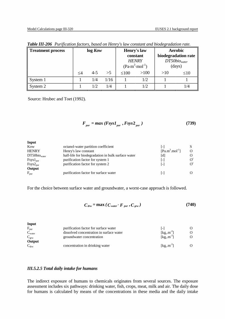
Model Calculations page III-320 EUSES 2.1 background report
Input Kow octanol-water partition coefficient [-] S HENRY Henry's law constant [Pa.m3.mol-1] O DT50biowater half-life for biodegradation in bulk surface water [d] O Fsys1pur purification factor for system 1 [-] Oc Fsys2pur purification factor for system 2 [-] Oc Output Fpur purification factor for surface water [-] O For the choice between surface water and groundwater, a worst-case approach is followed.
Input Fpur purification factor for surface water [-] O Cwater dissolved concentration in surface water [kgc.m-3] O Cgrw groundwater concentration [kgc.m-3] O Output Cdrw concentration in drinking water [kgc.m-3] O
III.5.2.5 Total daily intake for humans The indirect exposure of humans to chemicals originates from several sources. The exposure assessment includes six pathways: drinking water, fish, crops, meat, milk and air. The daily dose for humans is calculated by means of the concentrations in these media and the daily intake
Table III-206 Purification factors, based on Henry's law constant and biodegradation rate. Treatment process log Kow Henry's law
constant HENRY
(Pa⋅m3⋅mol-1)
Aerobic biodegradation rate
DT50biowater (days)
≤4 4-5 >5 ≤100 >100 >10 ≤10 System 1 1 1/4 1/16 1 1/2 1 1 System 2 1 1/2 1/4 1 1/2 1 1/4
Source: Hrubec and Toet (1992).
) Fsys, (Fsys1 max= F purpurpur 2 (739)
)C , F C( = C grwpurwaterdrw ⋅max (740)
EUSES 2.1 background report Model Calculations page III-321
values. This approach implies an exposure scenario whereby each of these intake media is retrieved exclusively from within the contaminated system.
The total dose can now be calculated as the sum of the dose for each medium:
The contribution of each intake medium to the total dose is calculated as:
Input Cdrw concentration in drinking water [kgc.m-3] O Cfish concentration in fish [kgc.kgwwt
-1] O Cleaf concentration in leaves of crops [kgc.kgwwt
-1] O Croot concentration in roots of crops [kgc.kgwwt
-1] O Cmeat concentration in meat [kgc.kgwwt
-1] O Cmilk concentration in milk [kgc.kgwwt
-1] O Cair concentration in air [kgc.mair
-3] O Fresp respirable fraction of inhaled substance [-] D IHi daily intake of medium i [kg.d-1 or m3.d-1] D BIOoral,2 bioavailability for oral intake [-] D BIOinh,2 bioavailability for inhalation [-] D BW body weight of (adult) human considered [kg] D Output DOSEi daily dose via intake of i [kgc.kgbw
-1.d-1] Oc DOSEtot total daily intake for humans [kgc.kgbw
-1.d-1] O Fdosei fraction of total dose via intake of medium i [-] Oc In Table III-207, the default consumption rates for each food product are given (taken from ECETOC, 1994). These values represent the highest country-average intake across all EU Member States for each food product.
milk}meat,root,leaf,fish,{drw, j BW
IH C= DOSE jjj ∈
⋅ (741)
2,
2,
oral
inhairairrespair BIO
BIO
BWIH C F= DOSE ⋅⋅⋅
(742)
milk}meat,root,leaf,fish,drw,{air, i
DOSE = DOSE ii
tot
∈
∑ (743)
DOSE
DOSE= Fdosei
i
ii ∑
(744)

Model Calculations page III-322 EUSES 2.1 background report
Table III-207 Standard defaults for indirect exposure of humans.
Parameter Symbol Value Unit Source
Daily intake of drinking water IHdrw 0.002 [m3.d-1] (b)
Daily intake of fish IHfish 0.115 [kgwwt.d-1] (a)
Daily intake of leaf crops (incl. fruit and cereals) IHleaf 1.20 [kgwwt.d-1] (a)
Daily intake of root crops IHroot 0.384 [kgwwt.d-1] (a)
Daily intake of meat IHmeat 0.301 [kgwwt.d-1] (a)
Daily intake of dairy products IHmilk 0.561 [kgwwt.d-1] (a)
Daily inhalation rate IHair 20 [m3.d-1] (b)
Respirable fraction of the inhaled substance Fresp 1 [-]
Bioavailability for inhalation BIOinh 0.75 [-] (c)
Bioavailability for oral uptake BIOoral 1.0 [-] (c)
Body weight of adult BW 70 [kg]
a Source: Euromonitor (1992) as reported by ECETOC (1994). b Source: US-EPA (1989). c Source: Vermeire et al. (1993b).
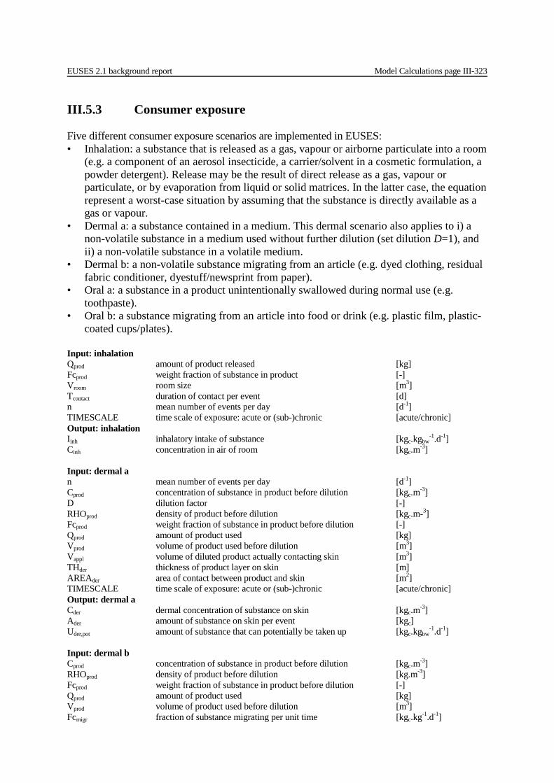
EUSES 2.1 background report Model Calculations page III-323
III.5.3 Consumer exposure Five different consumer exposure scenarios are implemented in EUSES: • Inhalation: a substance that is released as a gas, vapour or airborne particulate into a room
(e.g. a component of an aerosol insecticide, a carrier/solvent in a cosmetic formulation, a powder detergent). Release may be the result of direct release as a gas, vapour or particulate, or by evaporation from liquid or solid matrices. In the latter case, the equation represent a worst-case situation by assuming that the substance is directly available as a gas or vapour.
• Dermal a: a substance contained in a medium. This dermal scenario also applies to i) a non-volatile substance in a medium used without further dilution (set dilution D=1), and ii) a non-volatile substance in a volatile medium.
• Dermal b: a non-volatile substance migrating from an article (e.g. dyed clothing, residual fabric conditioner, dyestuff/newsprint from paper).
• Oral a: a substance in a product unintentionally swallowed during normal use (e.g. toothpaste).
• Oral b: a substance migrating from an article into food or drink (e.g. plastic film, plastic-coated cups/plates).
Input: inhalation Qprod amount of product released [kg] Fcprod weight fraction of substance in product [-] Vroom room size [m3] Tcontact duration of contact per event [d] n mean number of events per day [d-1] TIMESCALE time scale of exposure: acute or (sub-)chronic [acute/chronic] Output: inhalation Iinh inhalatory intake of substance [kgc.kgbw
-1.d-1] Cinh concentration in air of room [kgc.m-3] Input: dermal a n mean number of events per day [d-1] Cprod concentration of substance in product before dilution [kgc.m-3] D dilution factor [-] RHOprod density of product before dilution [kgc.m-3] Fcprod weight fraction of substance in product before dilution [-] Qprod amount of product used [kg] Vprod volume of product used before dilution [m3] Vappl volume of diluted product actually contacting skin [m3] THder thickness of product layer on skin [m] AREAder area of contact between product and skin [m2] TIMESCALE time scale of exposure: acute or (sub-)chronic [acute/chronic] Output: dermal a Cder dermal concentration of substance on skin [kgc.m-3] Ader amount of substance on skin per event [kgc] Uder,pot amount of substance that can potentially be taken up [kgc.kgbw
-1.d-1] Input: dermal b Cprod concentration of substance in product before dilution [kgc.m-3] RHOprod density of product before dilution [kg.m-3] Fcprod weight fraction of substance in product before dilution [-] Qprod amount of product used [kg] Vprod volume of product used before dilution [m3] Fcmigr fraction of substance migrating per unit time [kgc.kg-1.d-1]
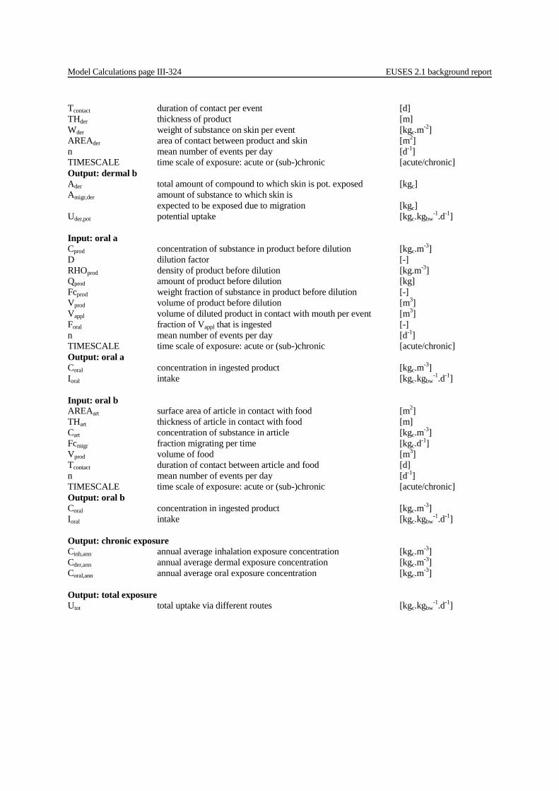
Model Calculations page III-324 EUSES 2.1 background report
Tcontact duration of contact per event [d] THder thickness of product [m] Wder weight of substance on skin per event [kgc.m-2] AREAder area of contact between product and skin [m2] n mean number of events per day [d-1] TIMESCALE time scale of exposure: acute or (sub-)chronic [acute/chronic] Output: dermal b Ader total amount of compound to which skin is pot. exposed [kgc] Amigr,der amount of substance to which skin is expected to be exposed due to migration [kgc] Uder,pot potential uptake [kgc.kgbw
-1.d-1] Input: oral a Cprod concentration of substance in product before dilution [kgc.m-3] D dilution factor [-] RHOprod density of product before dilution [kg.m-3] Qprod amount of product before dilution [kg] Fcprod weight fraction of substance in product before dilution [-] Vprod volume of product before dilution [m3] Vappl volume of diluted product in contact with mouth per event [m3] Foral fraction of Vappl that is ingested [-] n mean number of events per day [d-1] TIMESCALE time scale of exposure: acute or (sub-)chronic [acute/chronic] Output: oral a Coral concentration in ingested product [kgc.m-3] Ioral intake [kgc.kgbw
-1.d-1] Input: oral b AREAart surface area of article in contact with food [m2] THart thickness of article in contact with food [m] Cart concentration of substance in article [kgc.m-3] Fcmigr fraction migrating per time [kgc.d-1] Vprod volume of food [m3] Tcontact duration of contact between article and food [d] n mean number of events per day [d-1] TIMESCALE time scale of exposure: acute or (sub-)chronic [acute/chronic] Output: oral b Coral concentration in ingested product [kgc.m-3] Ioral intake [kgc.kgbw
-1.d-1] Output: chronic exposure Cinh,ann annual average inhalation exposure concentration [kgc.m-3] Cder,ann annual average dermal exposure concentration [kgc.m-3] Coral,ann annual average oral exposure concentration [kgc.m-3] Output: total exposure Utot total uptake via different routes [kgc.kgbw
-1.d-1]
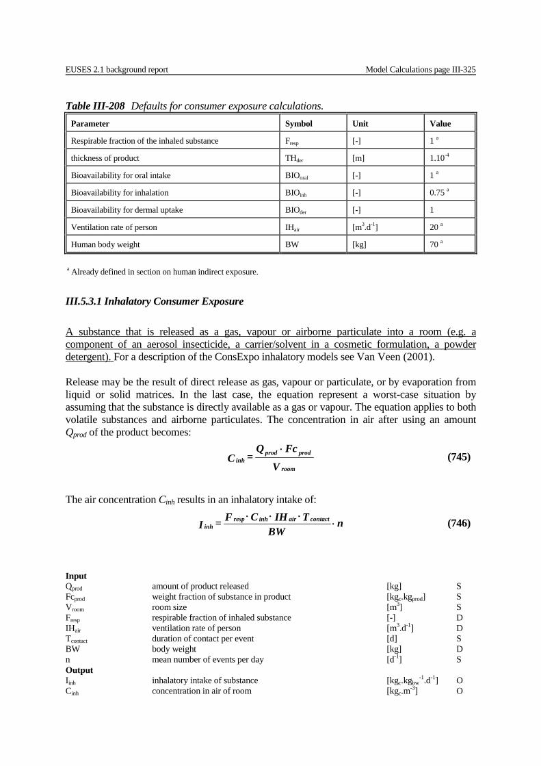
EUSES 2.1 background report Model Calculations page III-325
III.5.3.1 Inhalatory Consumer Exposure A substance that is released as a gas, vapour or airborne particulate into a room (e.g. a component of an aerosol insecticide, a carrier/solvent in a cosmetic formulation, a powder detergent). For a description of the ConsExpo inhalatory models see Van Veen (2001). Release may be the result of direct release as gas, vapour or particulate, or by evaporation from liquid or solid matrices. In the last case, the equation represent a worst-case situation by assuming that the substance is directly available as a gas or vapour. The equation applies to both volatile substances and airborne particulates. The concentration in air after using an amount Qprod of the product becomes:
The air concentration Cinh results in an inhalatory intake of:
Input Qprod amount of product released [kg] S Fcprod weight fraction of substance in product [kgc.kgprod] S Vroom room size [m3] S Fresp respirable fraction of inhaled substance [-] D IHair ventilation rate of person [m3.d-1] D Tcontact duration of contact per event [d] S BW body weight [kg] D n mean number of events per day [d-1] S Output Iinh inhalatory intake of substance [kgc.kgbw
-1.d-1] O Cinh concentration in air of room [kgc.m-3] O
Table III-208 Defaults for consumer exposure calculations. Parameter Symbol Unit Value
Respirable fraction of the inhaled substance Fresp [-] 1 a
thickness of product THder [m] 1.10-4
Bioavailability for oral intake BIOoral [-] 1 a
Bioavailability for inhalation BIOinh [-] 0.75 a
Bioavailability for dermal uptake BIOder [-] 1
Ventilation rate of person IHair [m3.d-1] 20 a
Human body weight BW [kg] 70 a
a Already defined in section on human indirect exposure.
V
FcQ= C
room
prodprodinh
⋅ (745)
n BW
T IH C F= I contactairinhrespinh ⋅
⋅⋅⋅ (746)
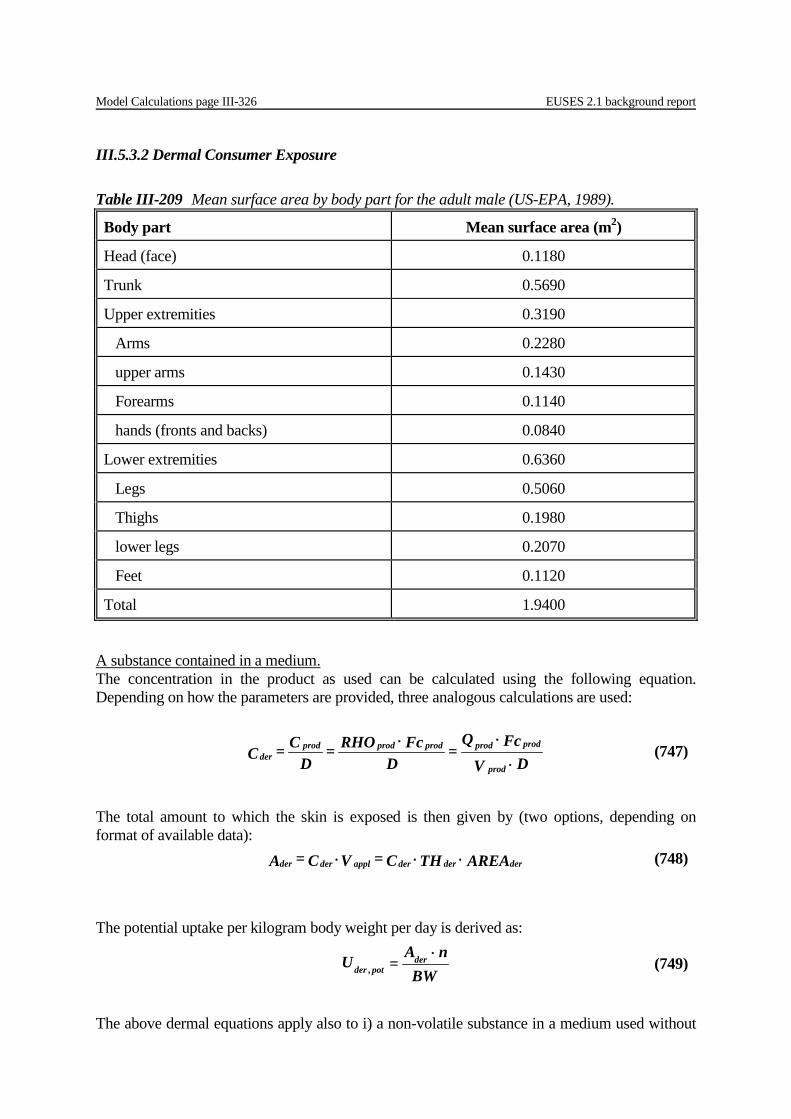
Model Calculations page III-326 EUSES 2.1 background report
III.5.3.2 Dermal Consumer Exposure
A substance contained in a medium. The concentration in the product as used can be calculated using the following equation. Depending on how the parameters are provided, three analogous calculations are used:
The total amount to which the skin is exposed is then given by (two options, depending on format of available data):
The potential uptake per kilogram body weight per day is derived as:
The above dermal equations apply also to i) a non-volatile substance in a medium used without
Table III-209 Mean surface area by body part for the adult male (US-EPA, 1989).
Body part Mean surface area (m2)
Head (face) 0.1180
Trunk 0.5690
Upper extremities 0.3190
Arms 0.2280
upper arms 0.1430
Forearms 0.1140
hands (fronts and backs) 0.0840
Lower extremities 0.6360
Legs 0.5060
Thighs 0.1980
lower legs 0.2070
Feet 0.1120
Total 1.9400
D V
Fc Q=
DFc RHO=
DC= C
prod
prodprodprodprodprodder ⋅
⋅⋅ (747)
AREA TH C= V C= A derderderapplderder ⋅⋅⋅ (748)
BW
nA= U der
pot,der
⋅ (749)
EUSES 2.1 background report Model Calculations page III-327
further dilution (set dilution D=1), and ii) a non-volatile substance in a volatile medium. In the latter case, the concentration Cder is valid at the very beginning of exposure only. However, this concentration can still be used to calculate Ader, because the substance is non-volatile. The above dermal equations can also be used in the case of a volatile substance, but in that case they represent a worst-case situation. If the duration of contact is specified, a chronic exposure can be calculated by EUSES (equation 221). For a description of the ConsExpo inhalatory models see Van Veen (2001). Input Cprod concentration of substance in product before dilution [kgc.m-3] S D dilution factor [-] S RHOprod density of product before dilution [kg.m-3] S Qprod amount of product used [kg] S Fcprod weight fraction of substance in product before dilution [-] S Vprod volume of product used before dilution [m3] S Vappl volume of diluted product actually contacting the skin [m3] S THder thickness of product layer on skin [m] D AREAder area of contact between product and skin [m2] P/S BW body weight [kg] D n mean number of events per day [d-1] S Output Cder dermal concentration of substance on skin [kgc.m-3] O Ader amount of substance on skin per event [kgc] O Uder,pot amount of substance that can potentially be taken up [kgc.kgbw
-1.d-1] O A non-volatile substance migrating from an article (e.g. dyed clothing, residual fabric conditioner, dyestuff/newsprint from paper). The exposure calculation will involve estimating the amount of substance which will migrate from the area of the article in contact with skin during the time of contact. The concentration in the product as used can be calculated according to Equation (209) in case the density of the product and the fraction of substance in the product are known. Dyestuff levels in fabrics and paper are usually given as weight of product per unit area (e.g. mg/m2). The total amount is then calculated by multiplying by AREAder. The amount to which the skin is exposed is given by
where Cder ⋅ THder is equal to weight per unit of area:
Extractability in simulated body fluids for several classes of dyestuffs and different fabric types has been evaluated by ETAD (1983). For migrating substances, only part of the total amount Ader is able to reach the skin. The amount to be used is:
where Fcmigr ⋅ Tcontact must be much smaller than 1. The potential uptake per kilogram body
AREA TH C= AREA W= A derderderderderder ⋅⋅⋅ (750)
TH C= W derderder ⋅ (751)
T Fc A= A contactmigrderdermigr, ⋅⋅ (752)

Model Calculations page III-328 EUSES 2.1 background report
weight per day is then derived as:
It should be noted that EUSES does not check whether the estimated daily uptake exceeds the theoretical maximum. This maximum can be derived from the amount of product used (kg), the concentration of the substance (kgc.kg-1) in the product, the use frequency (d-1) and the bodyweight (kgbw). EUSES also asks to specify the duraction of contact per event to be able to calculate a chronic dermal exposure. Input Fcmigr fraction of substance migrating per unit time [kgc.kg-1.d-1] S Tcontact duration of contact per event [d] S THder thickness of product [m] D Wder weight of substance on skin per event [kgc.m-2] S AREAder area of contact between product and skin [m2] P/S Cder concentration of substance [kgc.m-3] O BW body weight [kg] D n mean number of events per day [d-1] S Output Ader total amount of comp. to which skin is pot. exposed [kgc] O Amigr,der amount of substance to which skin is expected to be exposed due to migration [kgc] O Uder,pot potential uptake [kgc.kgbw
-1.d-1] O
III.5.3.3 Oral consumer exposure A substance in a product unintentionally swallowed during normal use (e.g. toothpaste). These equations may also be used to estimate exposures arising from ingestion of the non-respirable fraction of inhaled airborne particulates. The concentration in the product as swallowed is calculated from
and the intake is then given by
If an undiluted product is swallowed, D = 1. For a description of the ConsExpo inhalatory models see Van Veen (2001).
BW
n A= U dermigr,potder,
⋅ (753)
D V
Fc Q=
DFc RHO=
DC= C
prod
prodprodprodprodprodoral ⋅
⋅⋅ (754)
BW
n C V F= I oralapploraloral
⋅⋅⋅ (755)
EUSES 2.1 background report Model Calculations page III-329
Input Cprod concentration of substance in product before dilution [kgc.m-3] S D dilution factor [-] S RHOprod density of product before dilution [kg.m-3] S Qprod amount of product before dilution [kgc] S Fcprod weight fraction of substance in product before dilution [-] S Vprod volume of product before dilution [m3] S Vappl volume of diluted product per event in contact with mouth [m3] S Foral fraction of Vappl that is ingested [-] S BW body weight [kg] D n mean number of events per day [d-1] S Output Coral concentration in ingested product [kgc.m-3] O Ioral intake [kgc.kgbw
-1.d-1] O A substance migrating from an article into food or drink (e.g. plastic film, plastic-coated cups/plates). The following equation can be used to obtain a conservative estimate of substance uptake from a defined volume of food. The value of Fcmigr will be influenced by the type of food (e.g. fatty/dry/moist), the period of exposure and the temperature at which migration occurs. The consumer exposure level will be influenced by the proportion of the contaminated food eaten. The concentration in the food as a result of migration from an article is given by:
Oral intake is given by:
Input AREAart surface area of article in contact with food [m2] S THart thickness of article in contact with food [m] S Cart concentration of substance in article [kgc.m-3] S Fcmigr fraction migrating per time [kgc.d-1] S Vprod volume of food [m3] S Vappl volume of diluted product actually ingested [m3] S Tcontact contact duration between article and food [d] S BW body weight [kg] D n mean number of events per day [d-1] S Output Coral concentration in ingested product [kgc.m-3] O Ioral intake [kgc.kgbw
-1.d-1] O
V
T Fc C TH AREA= Cprod
contactmigrartartartoral
⋅⋅⋅⋅ (756)
BW
n C V= I oralapploral
⋅⋅ (757)
Model Calculations page III-330 EUSES 2.1 background report
III.5.3.4 Acute versus chronic consumer exposure Consumer exposure may be acute or chronic. Because consumer products are used lifelong, the lifetime average exposure is well approximated by using the annual average exposure, averaging out seasonal usage differences. With regard to acute exposures, the equations used for consumer exposure model exposures as resulting from a constant concentration, thereby setting mean and maximum event concentrations equal. Therefore, acute exposure is characterized by the inhalatory, dermal, and oral concentrations, Cinh, Cder, and Coral respectively, which are given in the model descriptions. For chronic exposures, the intake and potential uptake rates Iinh, Uder,pot and Ioral represent annual average measures of exposure. Where chronic exposure is measured with reference to concentration, the annual average exposure concentrations are to be used:
where Croute represents the exposure concentration via the inhalatory, dermal or oral route. Both the acute and the chronic characterisation of exposure are given. The former is compared to the LD50, the latter to the chronic NOAEL. Because the equations model exposure with reference to constant concentration, the equation can be written as:
Input Croute exposure concentration through route route [kgc.m-3] O Tcontact event duration [d] S n mean number of events per day [d-1] S Output Cinh,ann annual average inhalation exposure concentration [kgc.m-3] O Cder,ann annual average dermal exposure concentration [kgc.m-3] O Coral,ann annual average oral exposure concentration [kgc.m-3] O Both the acute and the chronic characterisations are given per route. The acute concentrations are compared to the appropriate acute toxicity value, the chronic intakes or concentrations to the appropriate N(L)OAEL.
III.5.3.5 Total consumer exposure If a consumer is exposed to a substance in a particular consumer product via different routes, the contribution of each route to the total uptake can be summed. The summation is done for each time scale separately (acute and -sub-chronic). Differences in bioavailability for the various routes are accounted for by multiplying the intakes (or potential uptakes) with absolute absorption factors.
oral}der,{inh, route dt (t)C
=Croute
annroute, ∈∫
365
365
0 (758)
oral}der,{inh, route T n C= C contactrouteannroute, ∈⋅⋅ (759)
EUSES 2.1 background report Model Calculations page III-331
Input Iinh inhalatory intake of substance [kgc.kgbw
-1.d-1] O Uder,pot potential uptake [kgc.kgbw
-1.d-1] O Ioral intake [kgc.kgbw
-1.d-1] O BIOoral,2 bioavailability for oral intake (end route) [-] D BIOinh,2 bioavailability for inhalation (end route) [-] D BIOder,2 bioavailability for dermal uptake (end route) [-] D Output Utot total uptake for one product via different routes [kgc.kgbw
-1.d-1] O
III.5.3.6 ConsExpo ConsExpo 3.0 (Van Veen, 2001) can be started (or circumvented) from EUSES. When started the selected output of Consexpo is exported to EUSES and used in the further calculation General input data With the ConsExpo implements several exposure models for the inhalatory, dermal and oral routes of exposure resp. For all these scenarios the contact of the exposed person with the substance and the physico-chemical properties of the substance have to be defined: Input: contact use frequency [year-1] use duration [min] total duration [min] Input: chemical molecular weight [g.mol-1] octanol/water partition coefficient [number] vapour pressure [Pa] water solubility [g.liter-1] ConsExpo: inhalatory models ConsExpo implements the EUSES inhalatory model as the “constant concentration”-scenario. In addition ConsExpo implements five more advanced inhalatory scenarios. • source-ventilation : a substance is released into the (ventilated) room air with a constant
release rate. • evaporation from pure substance: a substance is released from a open can filled with the
(liquid) substance in it’s pure form by evaporation. • evaporation from mixture: a substance is released by evaporation from a open can filled
with a liquid mixture of which the substance is an ingredient. • painting: a viscous product such as paint is being applied to a surface with a certain
application area. The substance, which is part of the paint, diffuses to the surface of the applied product and evaporates.
• spray: currently being revised. Input: source and ventilation generation (/release) rate of the substance [kgc .s-1] break down rate of the substance [s-1]
BIO I + BIO U + BIO I = U oraloralderpotder,inhinhtot 2,2,2, ⋅⋅⋅ (760)
Model Calculations page III-332 EUSES 2.1 background report
room volume [m3] ventilation rate [h-1] ambient air concentration [kgc.m-3] Input: evaporation from pure substance model release area [m2] temperature [oC] room volume [m3] ventilation rate [m3.h-1] Input: evaporation from mixture model release area [m2] temperature [oC] room volume [m3] ventilation rate [h-1] molecular weight matrix product [kg.mol-1] weight fraction of the substance in the product [fraction] Input: painting model release area [m2] product amount [g] weight fraction of the substance in the product [fraction] density product [kg.m-3] layer exchange rate [min-1] fraction upper layer [fraction] room volume [m3] ventilation rate [h-1] temperature [oC] molecular weight matrix product [kg.mol-1] Input: spray model Currently being revised ConsExpo offers three uptake models to calculate the internal dose for the inhalatory route: • Fraction model: a (user-)specified fraction of the exposure enters the body • Diffusion model: • Flow model Input: fraction model inhalation rate [m3.min-1] absorbed fraction [fraction] (should be 1 to calculate potential dose) respirable fraction [fraction] Input: diffusion model air/blood partition coefficient [ratio] blood flow [cm3.min-1] volume lung blood [cm3] lung wall permeability [cm.min-1] lung volume [liter] dead space [fraction] inhalation rate [liter.min-1] respirable fraction [fraction] Input: flow model air/blood partition coefficient [fraction] blood flow [cm3.s-1] inhalation rate [liter.min-1] respirable fraction [fraction]
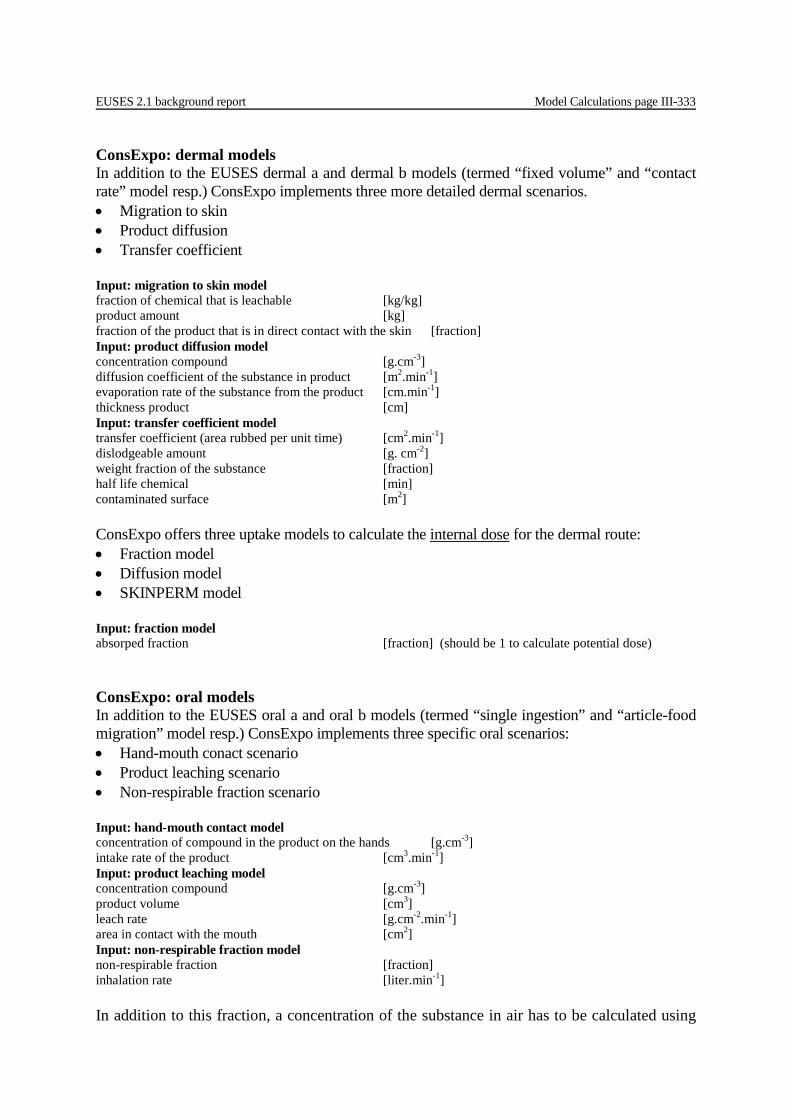
EUSES 2.1 background report Model Calculations page III-333
ConsExpo: dermal models In addition to the EUSES dermal a and dermal b models (termed “fixed volume” and “contact rate” model resp.) ConsExpo implements three more detailed dermal scenarios. • Migration to skin • Product diffusion • Transfer coefficient Input: migration to skin model fraction of chemical that is leachable [kg/kg] product amount [kg] fraction of the product that is in direct contact with the skin [fraction] Input: product diffusion model concentration compound [g.cm-3] diffusion coefficient of the substance in product [m2.min-1] evaporation rate of the substance from the product [cm.min-1] thickness product [cm] Input: transfer coefficient model transfer coefficient (area rubbed per unit time) [cm2.min-1] dislodgeable amount [g. cm-2] weight fraction of the substance [fraction] half life chemical [min] contaminated surface [m2] ConsExpo offers three uptake models to calculate the internal dose for the dermal route: • Fraction model • Diffusion model • SKINPERM model Input: fraction model absorped fraction [fraction] (should be 1 to calculate potential dose) ConsExpo: oral models In addition to the EUSES oral a and oral b models (termed “single ingestion” and “article-food migration” model resp.) ConsExpo implements three specific oral scenarios: • Hand-mouth conact scenario • Product leaching scenario • Non-respirable fraction scenario Input: hand-mouth contact model concentration of compound in the product on the hands [g.cm-3] intake rate of the product [cm3.min-1] Input: product leaching model concentration compound [g.cm-3] product volume [cm3] leach rate [g.cm-2.min-1] area in contact with the mouth [cm2] Input: non-respirable fraction model non-respirable fraction [fraction] inhalation rate [liter.min-1] In addition to this fraction, a concentration of the substance in air has to be calculated using
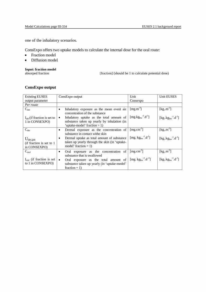
Model Calculations page III-334 EUSES 2.1 background report
one of the inhalatory scenarios. ConsExpo offers two uptake models to calculate the internal dose for the oral route: • Fraction model • Diffusion model Input: fraction model absorped fraction [fraction] (should be 1 to calculate potential dose) ConsExpo output Existing EUSES output parameter
ConsExpo output Unit Consexpo
Unit EUSES
Per route Cinh Iinh (if fraction is set to 1 in CONSEXPO)
• Inhalatory exposure as the mean event air concentration of the substance
• Inhalatory uptake as the total amount of substance taken up yearly by inhalation (in ‘uptake-model’ fraction = 1)
[mg.m-3] [mg.kgbw
-1.d-1]
[kgc.m-3] [kgc.kgbw
-1.d-1]
Cder Uder,pot (if fraction is set to 1 in CONSEXPO)
• Dermal exposure as the concentration of substance in contact withe skin
• Dermal uptake as total amount of substance taken up yearly through the skin (in ‘uptake-model’ fraction = 1)
[mg.cm-3] [mg. kgbw
-1.d-1]
[kgc.m-3] [kgc.kgbw
-1.d-1]
Coral Ioral (if fraction is set to 1 in CONSEXPO)
• Oral exposure as the concentration of substance that is swallowed
• Oral exposure as the total amount of substance taken up yearly (in ‘uptake-model’ fraction = 1)
[mg.cm-3] [mg. kgbw
-1.d -1]
[kgc.m-3] [kgc.kgbw
-1.d-1]
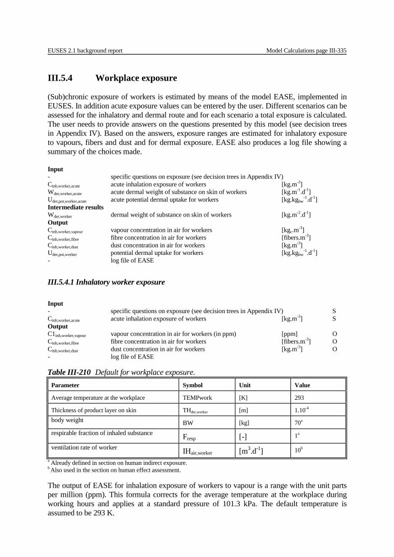
EUSES 2.1 background report Model Calculations page III-335
III.5.4 Workplace exposure (Sub)chronic exposure of workers is estimated by means of the model EASE, implemented in EUSES. In addition acute exposure values can be entered by the user. Different scenarios can be assessed for the inhalatory and dermal route and for each scenario a total exposure is calculated. The user needs to provide answers on the questions presented by this model (see decision trees in Appendix IV). Based on the answers, exposure ranges are estimated for inhalatory exposure to vapours, fibers and dust and for dermal exposure. EASE also produces a log file showing a summary of the choices made. Input - specific questions on exposure (see decision trees in Appendix IV) Cinh,worker,acute acute inhalation exposure of workers [kg.m-3] Wder,worker,acute acute dermal weight of substance on skin of workers [kg.m-1.d-1] Uder,pot,worker,acute acute potential dermal uptake for workers [kg.kgbw
-1.d-1] Intermediate results Wder,worker dermal weight of substance on skin of workers [kg.m-2.d-1] Output Cinh,worker,vapour vapour concentration in air for workers [kgc.m-3] Cinh,worker,fibre fibre concentration in air for workers [fibers.m-3] Cinh,worker,dust dust concentration in air for workers [kg.m-3] Uder,pot,worker potential dermal uptake for workers [kg.kgbw
-1.d-1] - log file of EASE
III.5.4.1 Inhalatory worker exposure Input - specific questions on exposure (see decision trees in Appendix IV) S Cinh,worker,acute acute inhalation exposure of workers [kg.m-3] S Output C1inh,worker,vapour vapour concentration in air for workers (in ppm) [ppm] O Cinh,worker,fibre fibre concentration in air for workers [fibers.m-3] O Cinh,worker,dust dust concentration in air for workers [kg.m-3] O - log file of EASE
a Already defined in section on human indirect exposure. b Also used in the section on human effect assessment. The output of EASE for inhalation exposure of workers to vapour is a range with the unit parts per million (ppm). This formula corrects for the average temperature at the workplace during working hours and applies at a standard pressure of 101.3 kPa. The default temperature is assumed to be 293 K.
Table III-210 Default for workplace exposure. Parameter Symbol Unit Value
Average temperature at the workplace TEMPwork [K] 293
Thickness of product layer on skin THder,worker [m] 1.10-4 body weight BW [kg] 70a respirable fraction of inhaled substance Fresp [-] 1a
ventilation rate of worker IHair,worker [m3.d-1] 10b
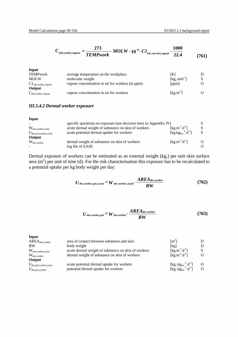
Model Calculations page III-336 EUSES 2.1 background report
Input TEMPwork average temperature on the workplace [K] D MOLW molecular weight [kgc.mol-1] S C1inh,worker,vapour vapour concentration in air for workers (in ppm) [ppm] O Output Cinh,worker,vapour vapour concentration in air for workers [kg.m-3] O
III.5.4.2 Dermal worker exposure Input - specific questions on exposure (see decision trees in Appendix IV) S Wder,worker,acute acute dermal weight of substance on skin of workers [kg.m-1.d-1] S Uder,pot,worker,acute acute potential dermal uptake for workers [kg.kgbw
-1.d-1] S Output Wder,worker dermal weight of substance on skin of workers [kg.m-2.d-1] O - log file of EASE O Dermal exposure of workers can be estimated as an external weight (kgc) per unit skin surface area (m2) per unit of time (d). For the risk characterisation this exposure has to be recalculated to a potential uptake per kg body weight per day:
Input AREAder,worker area of contact between substance and skin [m2] D BW body weight [kg] D Wder,worker,acute acute dermal weight of substance on skin of workers [kg.m-1.d-1] S Wder,worker dermal weight of substance on skin of workers [kg.m-2.d-1] O Output Uder,pot,worker,acute acute potential dermal uptake for workers [kgc.kgbw
-1.d-1] O Uder,pot,worker potential dermal uptake for workers [kgc.kgbw
-1.d-1] O
4221000
10273 6
. C1 MOLW
TEMPwork= C
vapourker,wor,inhvapour,inh,worker ⋅⋅⋅⋅ −
(761)
BW
AREA W= U workerder,acuteworkerder,acutepotworker,der, ⋅,, (762)
BW
AREA W= U der,workerder,workerpot,der,worker ⋅ (763)

EUSES 2.1 background report Model Calculations page III-337
III.5.4.3 Total worker exposure If a worker is exposed to a substance via different routes, the contribution of each route to the total uptake can be summed. The summation is done for each time scale separately (acute and –sub-chronic). Differences in bioavailability for the inhalatory and dermal routes are accounted for by multiplying the intakes (or potential uptakes) with absolute absorption factors. The vapour exposure concentrations for workers are recalculated to intakes:
n BW
T IH C F= Iworcontactworairacuteworinhresp
acuteworinh ⋅⋅⋅⋅ ker,ker,ker,,
ker,, (764)
n BW
T IH C F= Iworcontactworairvapourworinhresp
vapourworinh ⋅⋅⋅⋅ ker,ker,ker,,
ker,, (765)
Input Fresp respirable fraction of inhaled substance [-] D IHair,worker ventilation rate of worker [m3.d-1] D Tcontact,worker duration of contact with skin of worker per event [d] S BW body weight [kg] D n mean number of events per day [d-1] S Cinh,worker,acute acute inhalation exposure of workers [kg.m-3] S Cinh,worker,vapour vapour concentration in air for workers [kg.m-3] O Output Iinh,worker,acute acute inhalatory intake of substance for worker [kgc.kgbw
-1.d-1] O Iinh,worker, vapour inhalatory intake of substance for worker [kgc.kgbw
-1.d-1] O
BIO U + BIO I= U derworpotder,inhvapourworinhwordvtot ⋅⋅− ker,ker,,ker,/ (766)
BIO U + BIO I= U deracuteworpotder,inhacuteworinhacutewortot ⋅⋅ ker,,ker,,ker,, (767)

Model Calculations page III-338 EUSES 2.1 background report
Input Iinh,worker,acute acute inhalatory intake of substance for worker [kgc.kgbw
-1.d-1] O Iinh,worker, vapour inhalatory intake of substance for worker [kgc.kgbw
-1.d-1] O BIOinh bioavailability for inhalation [-] D BIOder bioavailability for dermal uptake [-] D Uder,pot,worker,acute acute potential dermal uptake for workers [kg.kgbw
-1.d-1] O Uder,pot,worker potential dermal uptake for workers [kg.kgbw
-1.d-1] O Output Utot,worker,acute total uptake for one scenario via different routes, for acute effects [kgc.kgbw
-1.d-1] O Utot-v/d,worker total uptake (vapour + dermal) for one scenario via different routes [kgc.kgbw
-1.d-1] O
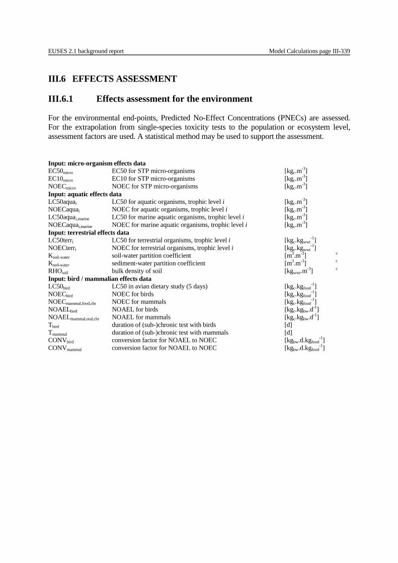
EUSES 2.1 background report Model Calculations page III-339
III.6 EFFECTS ASSESSMENT III.6.1 Effects assessment for the environment For the environmental end-points, Predicted No-Effect Concentrations (PNECs) are assessed. For the extrapolation from single-species toxicity tests to the population or ecosystem level, assessment factors are used. A statistical method may be used to support the assessment. Input: micro-organism effects data EC50micro EC50 for STP micro-organisms [kgc.m-3] EC10micro EC10 for STP micro-organisms [kgc.m-3] NOECmicro NOEC for STP micro-organisms [kgc.m-3] Input: aquatic effects data LC50aquai LC50 for aquatic organisms, trophic level i [kgc.m-3] NOECaquai NOEC for aquatic organisms, trophic level i [kgc.m-3] LC50aquai,marine LC50 for marine aquatic organisms, trophic level i [kgc.m-3] NOECaquai,marine NOEC for marine aquatic organisms, trophic level i [kgc.m-3] Input: terrestrial effects data LC50terri LC50 for terrestrial organisms, trophic level i [kgc.kgwwt
-1] NOECterri NOEC for terrestrial organisms, trophic level i [kgc.kgwwt
-1] Ksoil-water soil-water partition coefficient [m3.m-3] c Ksed-water sediment-water partition coefficient [m3.m-3] c RHOsoil bulk density of soil [kgwwt.m-3] c Input: bird / mammalian effects data LC50bird LC50 in avian dietary study (5 days) [kgc.kgfood
-1] NOECbird NOEC for birds [kgc.kgfood
-1] NOECmammal,food,chr NOEC for mammals [kgc.kgfood
-1] NOAELbird NOAEL for birds [kgc.kgbw.d-1] NOAELmammal,oral,chr NOAEL for mammals [kgc.kgbw.d-1] Tbird duration of (sub-)chronic test with birds [d] Tmammal duration of (sub-)chronic test with mammals [d] CONVbird conversion factor for NOAEL to NOEC [kgbw.d.kgfood
-1] CONVmammal conversion factor for NOAEL to NOEC [kgbw.d.kgfood
-1]

Model Calculations page III-340 EUSES 2.1 background report
Intermediate results 1 TOXaqua toxicological data used for extrapolation of PNEC [kgc.m-3] AFaqua assessment factor applied in extrapolation of aquatic PNEC [-] AFaquamarine assessment factor applied in extrapolation of marine PNEC [-] TOXmicro toxicological data used for extrapolation of PNEC [kgc.m-3] AFmicro assessment factor applied in extrapolation of PNEC [-] TOXoral toxicological data used for extrapolation of PNEC [kgc.kgfood
-1] AForal assessment factor applied in extrapolation of PNEC [-] Intermediate results 2 TOXterr toxicological data used for extrapolation of PNEC [kgc.kgwwt
-1] AFterr assessment factor applied in extrapolation of PNEC [-] EPterr equilibrium partitioning used for PNEC in soil? [yes/no] c EPsed equilibrium partitioning used for PNEC in sediment? [yes/no] c Output 1 PNECwater PNEC for aquatic organisms [kgc.m-3] c PNECwater,marine PNEC for marine aquatic organisms [kgc.m-3] c PNECmicro-organisms PNEC for STP micro-organisms [kgc.m-3] c PNECoral PNEC for secondary poisoning of birds and mammals [kgc.kgfood
-1] c PNECstatwater PNEC for aquatic organisms with statistical method [kgc.m-3] c PNECstatwater, marine PNEC for marine aquatic organisms with statistical method [kgc.m-3] c PNECstatsoil PNEC for terrestrial organisms with statistical method [kgc.m-3] c Output 2 PNECsoil PNEC for terrestrial organisms [kgc.kgwwt
-1] c PNECsed PNEC for sediment-dwelling organisms [kgc.kgwwt
-1] Table III-211 Default environmental characteristics soil and sediment in all scales
Sediment
Weight fraction of organic carbon soil solids Focsoil [kgoc.kgsolid-1] 0.02
Weight fraction of organic matter soil solids Fomsoil [kgom.kgsolid-1] 0.02
Weight fraction of organic carbon in fresh water and marine sediment Focsed [kgoc.kgsolid-1] 0.05
Weight fraction of organic matter in fresh water and marine sediment Fomsed [kgom.kgsolid-1] 0.05
III.6.1.1 Aquatic compartment (freshwater and marine environment) Depending on the available toxicity data for aquatic organisms, assessment factors are selected for extrapolating single-species toxicity tests to a PNEC for the water compartment. If intermittent release is identified for a stage of the life cycle, only short-term effects need to be considered for risk characterisation of that stage (only for the aquatic compartment). The following trophic levels are distinguished for the freshwater and marine environment: • algae (primary producers); • crustaceans / Daphnia (primary consumers); • fish (secondary consumers); • other species (e.g. decomposers). ( ) aquaLC50 = aquaLC50 imin min (768)
( ) NOECaqua = NOECaqua imin min (769)
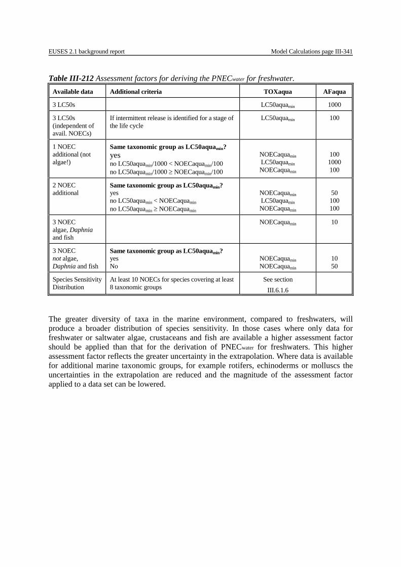
EUSES 2.1 background report Model Calculations page III-341
Table III-212 Assessment factors for deriving the PNECwater for freshwater. Available data Additional criteria TOXaqua AFaqua
3 LC50s LC50aquamin 1000
3 LC50s (independent of avail. NOECs)
If intermittent release is identified for a stage of the life cycle
LC50aquamin 100
1 NOEC additional (not algae!)
Same taxonomic group as LC50aquamin? yes no LC50aquamin/1000 < NOECaquamin/100 no LC50aquamin/1000 ≥ NOECaquamin/100
NOECaquamin LC50aquamin NOECaquamin
100 1000 100
2 NOEC additional
Same taxonomic group as LC50aquamin? yes no LC50aquamin < NOECaquamin no LC50aquamin ≥ NOECaquamin
NOECaquamin LC50aquamin NOECaquamin
50 100 100
3 NOEC algae, Daphnia and fish
NOECaquamin
10
3 NOEC not algae, Daphnia and fish
Same taxonomic group as LC50aquamin? yes No
NOECaquamin NOECaquamin
10 50
Species Sensitivity Distribution
At least 10 NOECs for species covering at least 8 taxonomic groups
See section III.6.1.6
The greater diversity of taxa in the marine environment, compared to freshwaters, will produce a broader distribution of species sensitivity. In those cases where only data for freshwater or saltwater algae, crustaceans and fish are available a higher assessment factor should be applied than that for the derivation of PNECwater for freshwaters. This higher assessment factor reflects the greater uncertainty in the extrapolation. Where data is available for additional marine taxonomic groups, for example rotifers, echinoderms or molluscs the uncertainties in the extrapolation are reduced and the magnitude of the assessment factor applied to a data set can be lowered.
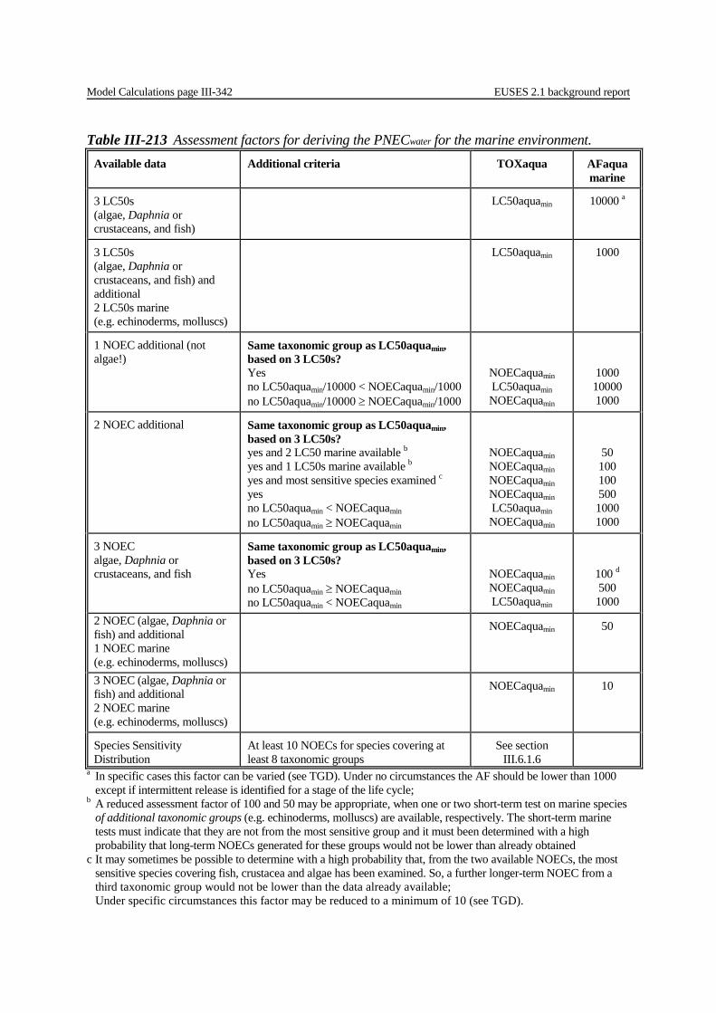
Model Calculations page III-342 EUSES 2.1 background report
Table III-213 Assessment factors for deriving the PNECwater for the marine environment. Available data Additional criteria TOXaqua AFaqua
marine
3 LC50s (algae, Daphnia or crustaceans, and fish)
LC50aquamin 10000 a
3 LC50s (algae, Daphnia or crustaceans, and fish) and additional 2 LC50s marine (e.g. echinoderms, molluscs)
LC50aquamin 1000
1 NOEC additional (not algae!)
Same taxonomic group as LC50aquamin, based on 3 LC50s? Yes no LC50aquamin/10000 < NOECaquamin/1000 no LC50aquamin/10000 ≥ NOECaquamin/1000
NOECaquamin LC50aquamin NOECaquamin
1000 10000 1000
2 NOEC additional Same taxonomic group as LC50aquamin, based on 3 LC50s? yes and 2 LC50 marine available b
yes and 1 LC50s marine available b yes and most sensitive species examined c yes no LC50aquamin < NOECaquamin no LC50aquamin ≥ NOECaquamin
NOECaquamin NOECaquamin NOECaquamin NOECaquamin LC50aquamin NOECaquamin
50 100 100 500 1000 1000
3 NOEC algae, Daphnia or crustaceans, and fish
Same taxonomic group as LC50aquamin, based on 3 LC50s? Yes no LC50aquamin ≥ NOECaquamin no LC50aquamin < NOECaquamin
NOECaquamin NOECaquamin LC50aquamin
100 d
500 1000
2 NOEC (algae, Daphnia or fish) and additional 1 NOEC marine (e.g. echinoderms, molluscs)
NOECaquamin
50
3 NOEC (algae, Daphnia or fish) and additional 2 NOEC marine (e.g. echinoderms, molluscs)
NOECaquamin
10
Species Sensitivity Distribution
At least 10 NOECs for species covering at least 8 taxonomic groups
See section III.6.1.6
a In specific cases this factor can be varied (see TGD). Under no circumstances the AF should be lower than 1000 except if intermittent release is identified for a stage of the life cycle;
b A reduced assessment factor of 100 and 50 may be appropriate, when one or two short-term test on marine species of additional taxonomic groups (e.g. echinoderms, molluscs) are available, respectively. The short-term marine tests must indicate that they are not from the most sensitive group and it must been determined with a high probability that long-term NOECs generated for these groups would not be lower than already obtained
c It may sometimes be possible to determine with a high probability that, from the two available NOECs, the most sensitive species covering fish, crustacea and algae has been examined. So, a further longer-term NOEC from a third taxonomic group would not be lower than the data already available;
Under specific circumstances this factor may be reduced to a minimum of 10 (see TGD).
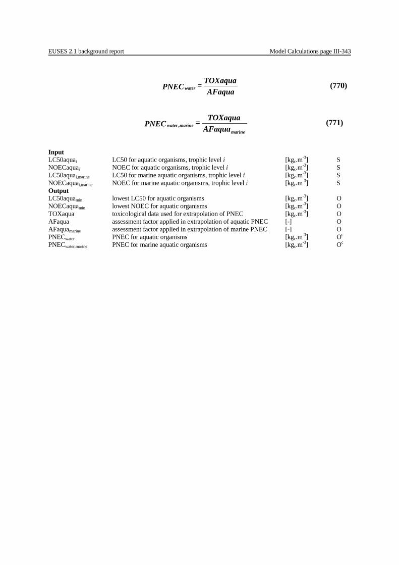
EUSES 2.1 background report Model Calculations page III-343
marine
marinewater AFaquaTOXaqua= PNEC , (771)
Input LC50aquai LC50 for aquatic organisms, trophic level i [kgc.m-3] S NOECaquai NOEC for aquatic organisms, trophic level i [kgc.m-3] S LC50aquai,marine LC50 for marine aquatic organisms, trophic level i [kgc.m-3] S NOECaquai,marine NOEC for marine aquatic organisms, trophic level i [kgc.m-3] S Output LC50aquamin lowest LC50 for aquatic organisms [kgc.m-3] O NOECaquamin lowest NOEC for aquatic organisms [kgc.m-3] O TOXaqua toxicological data used for extrapolation of PNEC [kgc.m-3] O AFaqua assessment factor applied in extrapolation of aquatic PNEC [-] O AFaquamarine assessment factor applied in extrapolation of marine PNEC [-] O PNECwater PNEC for aquatic organisms [kgc.m-3] Oc
PNECwater,marine PNEC for marine aquatic organisms [kgc.m-3] Oc
AFaqua
TOXaqua= PNECwater (770)
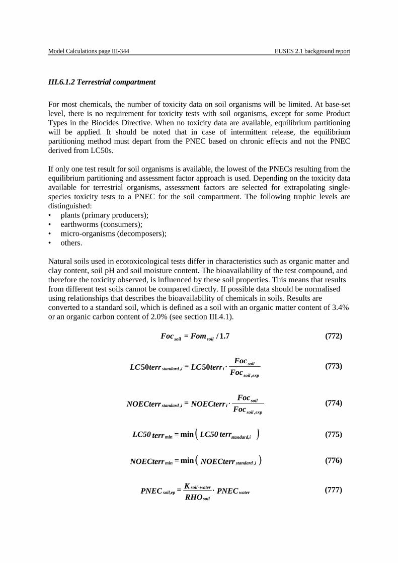
Model Calculations page III-344 EUSES 2.1 background report
III.6.1.2 Terrestrial compartment For most chemicals, the number of toxicity data on soil organisms will be limited. At base-set level, there is no requirement for toxicity tests with soil organisms, except for some Product Types in the Biocides Directive. When no toxicity data are available, equilibrium partitioning will be applied. It should be noted that in case of intermittent release, the equilibrium partitioning method must depart from the PNEC based on chronic effects and not the PNEC derived from LC50s. If only one test result for soil organisms is available, the lowest of the PNECs resulting from the equilibrium partitioning and assessment factor approach is used. Depending on the toxicity data available for terrestrial organisms, assessment factors are selected for extrapolating single-species toxicity tests to a PNEC for the soil compartment. The following trophic levels are distinguished: • plants (primary producers); • earthworms (consumers); • micro-organisms (decomposers); • others. Natural soils used in ecotoxicological tests differ in characteristics such as organic matter and clay content, soil pH and soil moisture content. The bioavailability of the test compound, and therefore the toxicity observed, is influenced by these soil properties. This means that results from different test soils cannot be compared directly. If possible data should be normalised using relationships that describes the bioavailability of chemicals in soils. Results are converted to a standard soil, which is defined as a soil with an organic matter content of 3.4% or an organic carbon content of 2.0% (see section III.4.1). 7.1/soilsoil = Fom Foc (772)
expsoil
soiliistandard Foc
Foc terrLC= terrLC
,, 5050 ⋅ (773)
expsoil
soiliistandard Foc
Foc NOECterr= NOECterr
,, ⋅ (774)
( ) terrLC50 = terrLC50 standard,imin min (775)
( ) NOECterr = NOECterr istandardmin ,min (776)
PNEC RHOK= PNEC water
soil
water-soilepsoil, ⋅ (777)
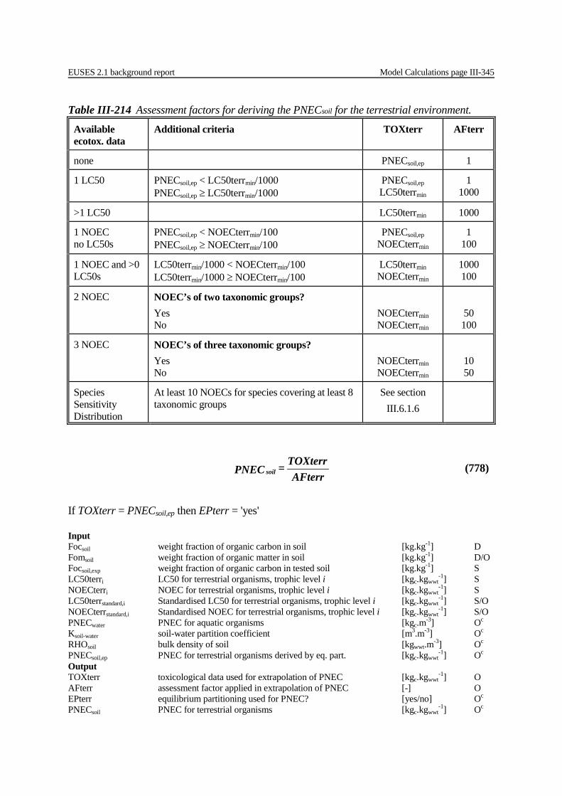
EUSES 2.1 background report Model Calculations page III-345
Table III-214 Assessment factors for deriving the PNECsoil for the terrestrial environment.
Available ecotox. data
Additional criteria TOXterr AFterr
none PNECsoil,ep 1
1 LC50 PNECsoil,ep < LC50terrmin/1000 PNECsoil,ep ≥ LC50terrmin/1000
PNECsoil,ep LC50terrmin
1 1000
>1 LC50 LC50terrmin 1000
1 NOEC no LC50s
PNECsoil,ep < NOECterrmin/100 PNECsoil,ep ≥ NOECterrmin/100
PNECsoil,ep NOECterrmin
1 100
1 NOEC and >0 LC50s
LC50terrmin/1000 < NOECterrmin/100 LC50terrmin/1000 ≥ NOECterrmin/100
LC50terrmin NOECterrmin
1000 100
2 NOEC NOEC’s of two taxonomic groups? Yes No
NOECterrmin NOECterrmin
50 100
3 NOEC NOEC’s of three taxonomic groups? Yes No
NOECterrmin NOECterrmin
10 50
Species Sensitivity Distribution
At least 10 NOECs for species covering at least 8 taxonomic groups
See section III.6.1.6
If TOXterr = PNECsoil,ep then EPterr = 'yes' Input Focsoil weight fraction of organic carbon in soil [kg.kg-1] D Fomsoil weight fraction of organic matter in soil [kg.kg-1] D/O Focsoil,exp weight fraction of organic carbon in tested soil [kg.kg-1] S LC50terri LC50 for terrestrial organisms, trophic level i [kgc.kgwwt
-1] S NOECterri NOEC for terrestrial organisms, trophic level i [kgc.kgwwt
-1] S LC50terrstandard,i Standardised LC50 for terrestrial organisms, trophic level i [kgc.kgwwt
-1] S/O NOECterrstandard,i Standardised NOEC for terrestrial organisms, trophic level i [kgc.kgwwt
-1] S/O PNECwater PNEC for aquatic organisms [kgc.m-3] Oc Ksoil-water soil-water partition coefficient [m3.m-3] Oc RHOsoil bulk density of soil [kgwwt.m-3] Oc PNECsoil,ep PNEC for terrestrial organisms derived by eq. part. [kgc.kgwwt
-1] Oc Output TOXterr toxicological data used for extrapolation of PNEC [kgc.kgwwt
-1] O AFterr assessment factor applied in extrapolation of PNEC [-] O EPterr equilibrium partitioning used for PNEC? [yes/no] Oc PNECsoil PNEC for terrestrial organisms [kgc.kgwwt
-1] Oc
AFterr
TOXterr= PNEC soil (778)
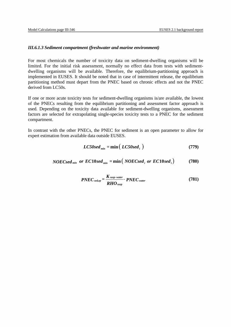
Model Calculations page III-346 EUSES 2.1 background report
III.6.1.3 Sediment compartment (freshwater and marine environment) For most chemicals the number of toxicity data on sediment-dwelling organisms will be limited. For the initial risk assessment, normally no effect data from tests with sediment-dwelling organisms will be available. Therefore, the equilibrium-partitioning approach is implemented in EUSES. It should be noted that in case of intermittent release, the equilibrium partitioning method must depart from the PNEC based on chronic effects and not the PNEC derived from LC50s. If one or more acute toxicity tests for sediment-dwelling organisms is/are available, the lowest of the PNECs resulting from the equilibrium partitioning and assessment factor approach is used. Depending on the toxicity data available for sediment-dwelling organisms, assessment factors are selected for extrapolating single-species toxicity tests to a PNEC for the sediment compartment. In contrast with the other PNECs, the PNEC for sediment is an open parameter to allow for expert estimation from available data outside EUSES. ( ) LC50sed = LC50sed imin min (779)
( )iiminmin sedECorNOECsed = sedECor NOECsed 10min10 (780)
PNEC RHOK= PNEC water
susp
water-suspepsed, ⋅ (781)
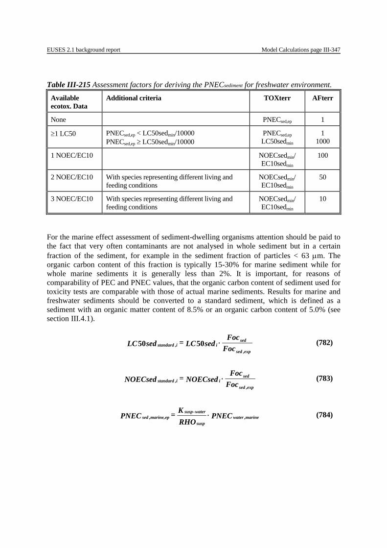
EUSES 2.1 background report Model Calculations page III-347
Table III-215 Assessment factors for deriving the PNECsediment for freshwater environment.
Available ecotox. Data
Additional criteria TOXterr AFterr
None PNECsed,ep 1
≥1 LC50 PNECsed,ep < LC50sedmin/10000 PNECsed,ep ≥ LC50sedmin/10000
PNECsed,ep LC50sedmin
1 1000
1 NOEC/EC10 NOECsedmin/ EC10sedmin
100
2 NOEC/EC10 With species representing different living and feeding conditions
NOECsedmin/ EC10sedmin
50
3 NOEC/EC10 With species representing different living and feeding conditions
NOECsedmin/ EC10sedmin
10
For the marine effect assessment of sediment-dwelling organisms attention should be paid to the fact that very often contaminants are not analysed in whole sediment but in a certain fraction of the sediment, for example in the sediment fraction of particles < 63 mm. The organic carbon content of this fraction is typically 15-30% for marine sediment while for whole marine sediments it is generally less than 2%. It is important, for reasons of comparability of PEC and PNEC values, that the organic carbon content of sediment used for toxicity tests are comparable with those of actual marine sediments. Results for marine and freshwater sediments should be converted to a standard sediment, which is defined as a sediment with an organic matter content of 8.5% or an organic carbon content of 5.0% (see section III.4.1).
expsed
sediistandard Foc
Foc sedLC= sedLC
,, 5050 ⋅ (782)
expsed
sediistandard Foc
Foc NOECsed= NOECsed
,, ⋅ (783)
PNEC RHOK= PNEC marinewater
susp
water-suspepmarine,sed ,, ⋅ (784)
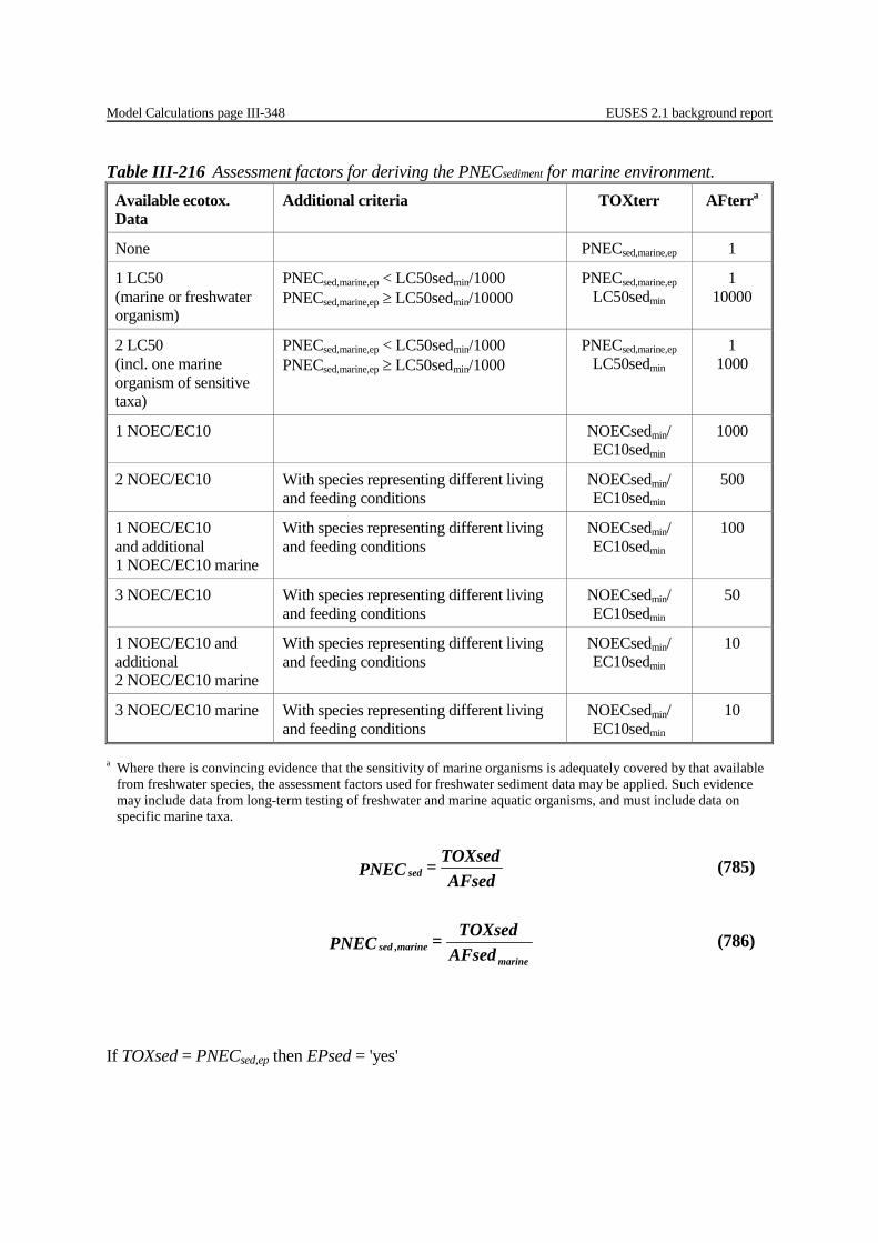
Model Calculations page III-348 EUSES 2.1 background report
Table III-216 Assessment factors for deriving the PNECsediment for marine environment. Available ecotox. Data
Additional criteria TOXterr AFterra
None PNECsed,marine,ep 1
1 LC50 (marine or freshwater organism)
PNECsed,marine,ep < LC50sedmin/1000 PNECsed,marine,ep ≥ LC50sedmin/10000
PNECsed,marine,ep LC50sedmin
1 10000
2 LC50 (incl. one marine organism of sensitive taxa)
PNECsed,marine,ep < LC50sedmin/1000 PNECsed,marine,ep ≥ LC50sedmin/1000
PNECsed,marine,ep LC50sedmin
1 1000
1 NOEC/EC10 NOECsedmin/ EC10sedmin
1000
2 NOEC/EC10 With species representing different living and feeding conditions
NOECsedmin/ EC10sedmin
500
1 NOEC/EC10 and additional 1 NOEC/EC10 marine
With species representing different living and feeding conditions
NOECsedmin/ EC10sedmin
100
3 NOEC/EC10 With species representing different living and feeding conditions
NOECsedmin/ EC10sedmin
50
1 NOEC/EC10 and additional 2 NOEC/EC10 marine
With species representing different living and feeding conditions
NOECsedmin/ EC10sedmin
10
3 NOEC/EC10 marine With species representing different living and feeding conditions
NOECsedmin/ EC10sedmin
10
a Where there is convincing evidence that the sensitivity of marine organisms is adequately covered by that available
from freshwater species, the assessment factors used for freshwater sediment data may be applied. Such evidence may include data from long-term testing of freshwater and marine aquatic organisms, and must include data on specific marine taxa.
AFsed
TOXsed= PNEC sed (785)
marine
marinesed AFsedTOXsed= PNEC , (786)
If TOXsed = PNECsed,ep then EPsed = 'yes'
EUSES 2.1 background report Model Calculations page III-349
Input Focsed weight fraction of organic carbon in marine sediment [kg.kg-1] D Fomsed weight fraction of organic matter in marine sediment [kg.kg-1] D/O Focsed,exp weight fraction of organic carbon in tested sediment [kg.kg-1] S LC50sedi LC50 for sediment-dwelling organisms, species i [kgc.kgwwt
-1] S NOECsedi NOEC for sediment-dwelling organisms, species i [kgc.kgwwt
-1] S EC10sedi EC10 for sediment-dwelling organisms, species i [kgc.kgwwt
-1] S LC50sedstandard,i Standardised LC50 for sediment-dwelling organisms, species i [kgc.kgwwt
-1] S/O NOECsedstandard,i Standardised NOEC for sediment-dwelling organisms, species i [kgc.kgwwt
-1] S/O EC10sedstandard,i Standardised EC10 for sediment-dwelling organisms, species i [kgc.kgwwt
-1] S/O PNECwater PNEC for aquatic organisms [kgc.m-3] Oc Ksusp-water suspended matter-water partition coefficient [m3.m-3] Oc RHOsusp bulk density of suspended matter [kgwwt.m-3] Oc PNECsed,ep PNEC for sediment-dwelling organisms derived by eq. part. [kgc.kgwwt
-1] Oc Output TOXsed toxicological data used for extrapolation of PNEC [kgc.kgwwt
-1] O AFsed assessment factor applied in extrapolation of PNEC [-] O EPsed equilibrium partitioning used for PNEC in sediment? [yes/no] Oc PNECsed PNEC for sediment-dwelling organisms [kgc.kgwwt
-1] O

Model Calculations page III-350 EUSES 2.1 background report
III.6.1.4 Micro-organisms Chemicals may cause adverse effects on microbial activity in STPs and therefore it is necessary to derive a PNECmicro-organisms. Current test systems for measuring the effect of chemicals on microbial activity have different endpoints and different levels of sensitivity. A number of internationally accepted test systems exist. Available data suggest the following order of increasing sensitivities among particular test systems: respiration inhibition test < inhibition control in base-set tests < growth inhibition test with P. putida < inhibition of nitrification. Depending on the test system and toxicity data available for micro-organisms, assessment factors are selected for extrapolating results from toxicity tests to a PNEC for the sewage treatment plant. Table III-217 Assessment factors for deriving the PNECmicro-organisms for the STP.
Test system TOXmicro AFmicro Activated sludge, respiration inhibition tests
Respiration inhibition tests EU Annex V C.11, OECD 209
NOECmicro or EC10micro 10
EC50micro 100 Inhibition control in base-set tests
Inhibition control in standard biodegradation test: ready or inherent tests
Tested conc. at which toxicity to inoculum can
be ruled out a
10
Activated sludge, other tests Activated sludge growth inhibition tests, ISO-15522
NOECmicro or EC10micro 10
EC50micro 100
Pilot scale activated sludge simulation tests OECD 303 A, ISO-11733
Expert judgement b Case-by-case down to 1
Tests with specific populations of bacteria or protozoa Inhibition of nitrification, ISO-9509
NOECmicro or EC10micro 1
EC50micro 10
Ciliate growth inhibition tests,
NOECmicro or EC10micro 1
EC50micro 10
Growth inhibition tests with Pseudomonas putida, NF EN ISO 10712
NOECmicro or EC10micro 1
EC50micro 10 a The tested concentration at which toxicity to the inoculum can be ruled out with sufficient reliability
(cf. corresponding text section above) could be considered as a NOEC for the toxicity to micro-organisms of a STP; b Based on case-by-case expert judgement, the tested concentration not impairing proper functioning of the
continuous activated sludge unit could be considered as NOEC for micro-organisms in STPs If more than one toxicity value is given, the lower of the resulting PNECs is used.
AFmicro
TOXmicro= PNEC organisms-micro (787)
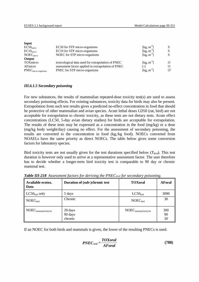
EUSES 2.1 background report Model Calculations page III-351
Input EC50micro EC50 for STP micro-organisms [kgc.m-3] S EC10micro EC10 for STP micro-organisms [kgc.m-3] S NOECmicro NOEC for STP micro-organisms [kgc.m-3] S Output TOXmicro toxicological data used for extrapolation of PNEC [kgc.m-3] O AFmicro assessment factor applied in extrapolation of PNEC [-] O PNECmicro-organisms PNEC for STP micro-organisms [kgc.m-3] Oc
III.6.1.5 Secondary poisoning For new substances, the results of mammalian repeated-dose toxicity test(s) are used to assess secondary poisoning effects. For existing substances, toxicity data for birds may also be present. Extrapolation from such test results gives a predicted no-effect concentration in food that should be protective of other mammalian and avian species. Acute lethal doses LD50 (rat, bird) are not acceptable for extrapolation to chronic toxicity, as these tests are not dietary tests. Acute effect concentrations (LC50, 5-day avian dietary studies) for birds are acceptable for extrapolation. The results of these tests may be expressed as a concentration in the food (mg/kg) or a dose (mg/kg body weight/day) causing no effect. For the assessment of secondary poisoning, the results are converted to the concentration in food (kgc/kg food). NOECs converted from NOAELs have the same priority as direct NOECs. The table below gives some conversion factors for laboratory species. Bird toxicity tests are not usually given for the test durations specified below (Tbird). This test duration is however only used to arrive at a representative assessment factor. The user therefore has to decide whether a longer-term bird toxicity test is comparable to 90 day or chronic mammal test. Table III-218 Assessment factors for deriving the PNECoral for secondary poisoning.
Available ecotox. Data
Duration of (sub-)chronic test TOXoral AForal
LC50bird only 5 days LC50bird 3000
NOECbird Chronic NOECbird 30
NOECmammal,food,chr 28 days 90 days chronic
NOECmammal,food,chr 300 90 30
If an NOEC for both birds and mammals is given, the lower of the resulting PNECs is used.
AForal
TOXoral= PNECoral (788)
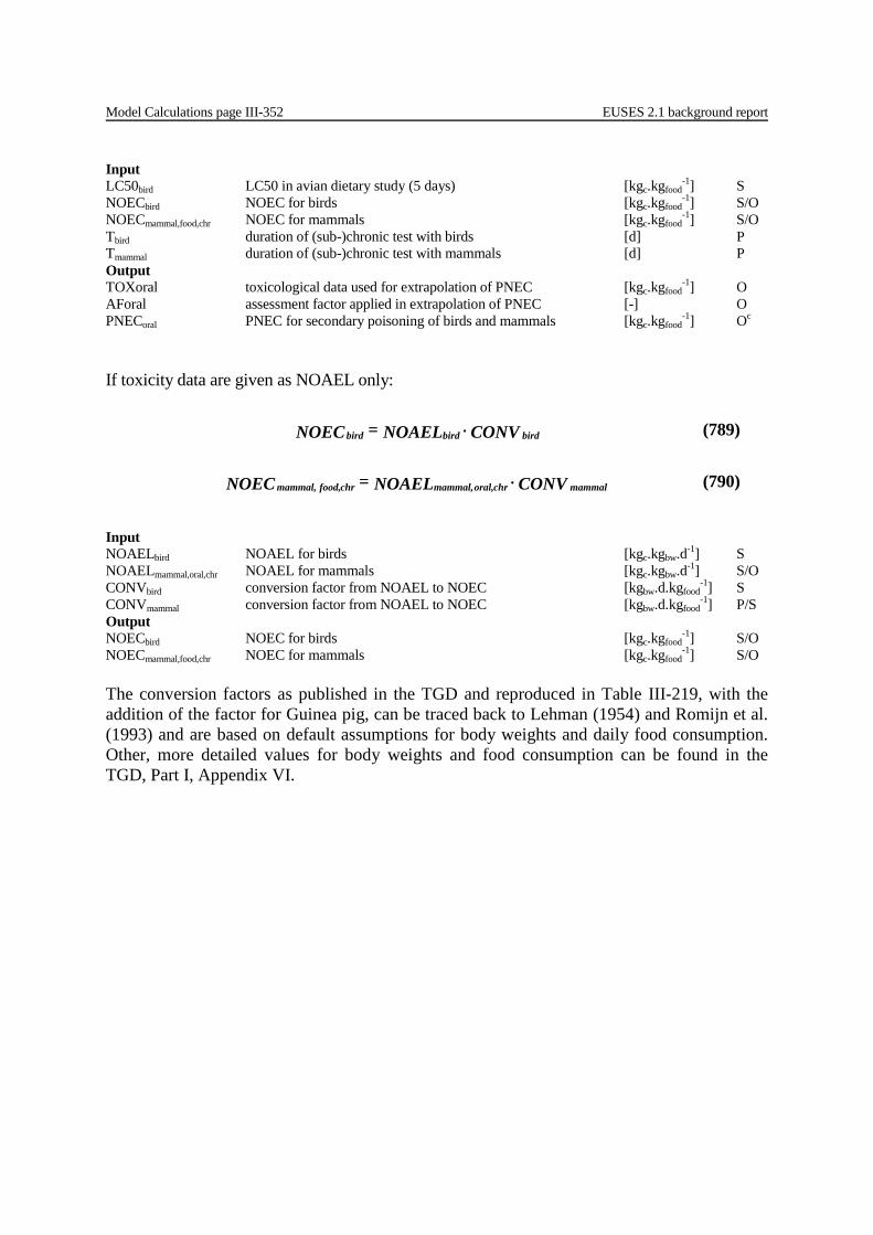
Model Calculations page III-352 EUSES 2.1 background report
Input LC50bird LC50 in avian dietary study (5 days) [kgc.kgfood
-1] S NOECbird NOEC for birds [kgc.kgfood
-1] S/O NOECmammal,food,chr NOEC for mammals [kgc.kgfood
-1] S/O Tbird duration of (sub-)chronic test with birds [d] P Tmammal duration of (sub-)chronic test with mammals [d] P Output TOXoral toxicological data used for extrapolation of PNEC [kgc.kgfood
-1] O AForal assessment factor applied in extrapolation of PNEC [-] O PNECoral PNEC for secondary poisoning of birds and mammals [kgc.kgfood
-1] Oc If toxicity data are given as NOAEL only:
Input NOAELbird NOAEL for birds [kgc.kgbw.d-1] S NOAELmammal,oral,chr NOAEL for mammals [kgc.kgbw.d-1] S/O CONVbird conversion factor from NOAEL to NOEC [kgbw.d.kgfood
-1] S CONVmammal conversion factor from NOAEL to NOEC [kgbw.d.kgfood
-1] P/S Output NOECbird NOEC for birds [kgc.kgfood
-1] S/O NOECmammal,food,chr NOEC for mammals [kgc.kgfood
-1] S/O The conversion factors as published in the TGD and reproduced in Table III-219, with the addition of the factor for Guinea pig, can be traced back to Lehman (1954) and Romijn et al. (1993) and are based on default assumptions for body weights and daily food consumption. Other, more detailed values for body weights and food consumption can be found in the TGD, Part I, Appendix VI.
CONV NOAEL= NOEC birdbirdbird ⋅ (789)
CONV NOAEL= NOEC mammalchroral,mammal,chrfood,mammal, ⋅ (790)

EUSES 2.1 background report Model Calculations page III-353
III.6.1.6 Statistical extrapolation method The statistical extrapolation method itself is not incorporated in EUSES 2.0. The Aldenberg and Jaworska (2000) method within the ETX-program (Van Vlaardingen and Traas, 2002) can be used to support the effect assessment performed with assessment factors. The results of this method can be entered as input (PNECstat). For the statistical extrapolation method we refer to the ETX-program, which can be obtained from the RIVM ([email protected]). The no-effect level (HC5) calculated according the Aldenberg and Jaworska (2000) method within ETX is the median concentration with the 90% confidence interval that protects 95% of the species in the system for which the experimental NOECs are a representative sample. The method is used for aquatic as well as terrestrial toxicity data. Values of the extrapolation constant ks depend on the number of NOECs given and the desired confidence level. According to the TGD (2003) at least 10 NOECs from at least 8 different taxonomic groups must be present for this calculation. The TGD lists the taxonomical groups that are required. The TGD also documents data selection and data averaging, if more than one NOEC is available for each species. In ETX it is checked whether the toxicity data deviate from the assumed normal distribution using the Anderson-Darling test (and the Kolmogorov Smirnov test). If a test statistic is above the 5% critical value, normality is rejected at the 5% critical value, indicating doubts about normality. If a GOF test statistic is below the 5% critical value, normality is accepted at the 5% critical value. If a higher critical value is accepted (e.g. at 2.5% significance level), then the probability that these data derive from a normal distribution is smaller than at 5%, but it is not impossible that the sample derives from a normal distribution. A GOF test does not say that a sample cannot derive from a normal distribution, just that it becomes less probable with decreasing significance levels.
Table III-219 Conversion factors from NOAEL to NOEC for several mammalian species.
Species Conversion factor (BW/DFI) CONVmammal [kgbw.d.kgfood
-1]
Canis domesticus/dog 40
Cavia cobaya/Guinea pig 25
Cricetus/hamster 10
Macaca spp./monkey 20
Microtus spp./vole 8.3
Mus musculus/mouse 8.3
Oryctolagus cuniculus/rabbit 33.3
Rattus norvegicus (> 6 weeks)/rat 20
Rattus norvegicus (≤ 6 weeks)/rat 10
Gallus domesticus/chick 8

Model Calculations page III-354 EUSES 2.1 background report
Input PNECstatwater PNEC for aquatic organisms with statistical method [kgc.m-3] S PNECstatwater, marine PNEC for marine aquatic organisms with statistical method [kgc.m-3] S PNECstatsoil PNEC for terrestrial organisms with statistical method [kgc.m-3] S
III.6.1.7 PBT assessment The PBT assessment (persistence, bioconcentration, toxicity) is not included in EUSES. It is referred to the TGD (2003) (Part II, chapter 4.4) for the criteria and the testing strategies.

EUSES 2.1 background report Model Calculations page III-355
III.6.2 Effects assessment for humans
III.6.2.1 Route-to-route extrapolation For acute time scale effects it is not common to perform route-to-route extrapolations. When necessary and applicable, for (sub-)chronic time scale effects (repeated dose toxicity, carcinogenicity and reproductive toxicity (and within this endpoint a.o. fertility, maternal toxicity and developmental toxicity) route-to-route extrapolations may be performed. Oral-to-dermal route If oral and dermal absorption rates are known these should be used in the calculations. If these data are not known default values should be taken.
Table III-220 Defaults for oral-to-dermal extrapolation. Parameter Symbol (a) Unit Value
Bioavailability for oral uptake BIOoral,1 [-] 1
Bioavailability for dermal uptake
MOLW >500 and [log Kow <-1 or >4] MOLW ≤500 and [log Kow ≥-1 or ≤4]
BIOder,2 [-]
0.10 1
These are parameters are already defined in the sub-modules on human exposure. (a) “1” indicates starting route, “2” end route.

Model Calculations page III-356 EUSES 2.1 background report
If absorption rates of humans and experimental animals differ and are known, the toxicity parameter estimated by EUSES should be corrected manually by multiplication with a factor BIOder-animal/BIOder-human. Input N(L)OAELmammal,oral,i oral N(L)OAEL for mammals for endpoint i [kgc.kgbw
-1.d-1] S/O N(L)OAELman,oral,i oral N(L)OAEL for man for endpoint i [kgc.kgbw
-1.d-1] S/O T25mammal,oral,nt oral T25 for mammals for non-threshold effects [kgc.kgbw
-1.d-1] S/O CEDmammal,oral,i oral CED for mammals for endpoint i [kgc.kgbw
-1.d-1] S/O i ∈ {repdose,carc,fert,mattox,devtox} CEDmammal,oral, nt oral CED for mammals for non-threshold effects [kgc.kgbw
-1.d-1] S/O BIOoral,1 bioavailability for oral uptake (starting route) [-] S/D BIOder,2 bioavailability for dermal uptake (end route) [-] S/D Output N(L)OAELmammal,der,i dermal N(L)OAEL for mammals for endpoint i [kgc.kgbw
-1.d-1] S/O N(L)OAELman,der,i dermal N(L)OAEL for man for endpoint i [kgc.kgbw
-1.d-1] S/O i ∈ {repdose,carc,fert,mattox,devtox} T25mammal,der,nt dermal T25 for mammals for non-threshold effects [kgc.kgbw
-1.d-1] S/O CEDmammal,der,i dermal CED for mammals for endpoint i [kgc.kgbw
-1.d-1] S/O i ∈ {repdose,carc,fert,mattox,devtox} CEDmammal,der, nt dermal CED for mammals for non-threshold effects [kgc.kgbw
-1.d-1] S/O
BIOBIO NOAEL= NOAEL
der
oralioral,mammal,ider,mammal,
2,
1,⋅ (791)
BIOBIO LOAEL= LOAEL
der
oralioral,mammal,ider,mammal,
2,
1,⋅ (792)
BIOBIO NOAEL= NOAEL
der
oralioral,man,ider,man,
2,
1,⋅ (793)
BIOBIO LOAEL= LOAEL
der
oralioral,man,ider,man,
2,
1,⋅ (794)
BIOBIO CED= CED
der
oralioralmammal,idermammal
2,
1,,,, ⋅ (795)
devtox}mattoxfertcarc{repdose i ,,,,∈
BIOBIO T= T
der
oralntoralmammalntdermammal
2,
1,,,,, 2525 ⋅ (796)
BIOBIO CED= CED
der
oralntoralmammal,ntdermammal
2,
1,,,, ⋅ (797)
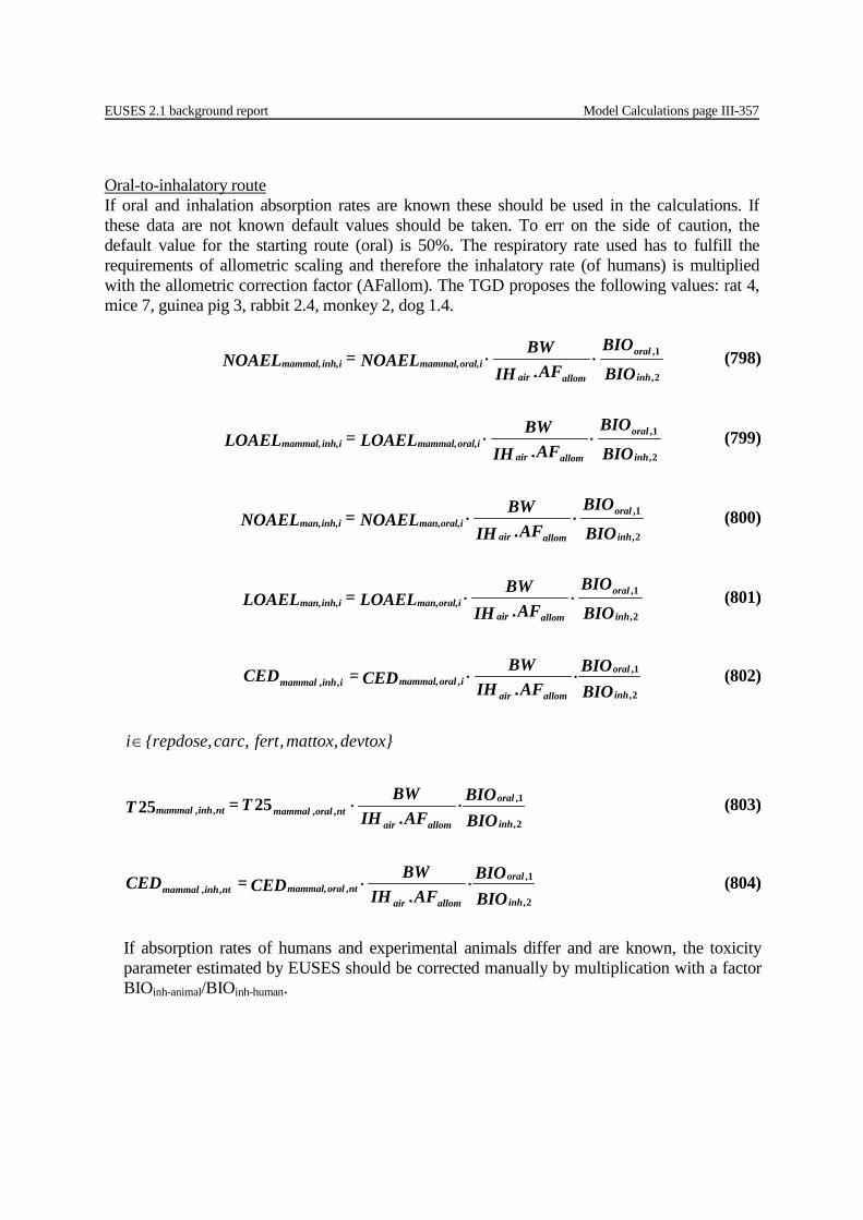
EUSES 2.1 background report Model Calculations page III-357
Oral-to-inhalatory route If oral and inhalation absorption rates are known these should be used in the calculations. If these data are not known default values should be taken. To err on the side of caution, the default value for the starting route (oral) is 50%. The respiratory rate used has to fulfill the requirements of allometric scaling and therefore the inhalatory rate (of humans) is multiplied with the allometric correction factor (AFallom). The TGD proposes the following values: rat 4, mice 7, guinea pig 3, rabbit 2.4, monkey 2, dog 1.4.
BIO
BIO
AFIHBW NOAEL= NOAEL
inh
oral
allomairioral,mammal,iinh,mammal,
2,
1,
.⋅⋅ (798)
BIO
BIO
AFIHBW LOAEL= LOAEL
inh
oral
allomairioral,mammal,iinh,mammal,
2,
1,
.⋅⋅ (799)
BIO
BIO
AFIHBW NOAEL= NOAEL
inh
oral
allomairioral,man,iinh,man,
2,
1,
.⋅⋅ (800)
BIO
BIO
AFIHBW LOAEL= LOAEL
inh
oral
allomairioral,man,iinh,man,
2,
1,
.⋅⋅ (801)
BIOBIO
AFIHBW CED= CED
inh
oral
allomairioralmammal,iinhmammal
2,
1,,,, .
⋅⋅ (802)
devtox}mattoxfertcarc{repdose i ,,,,∈
BIOBIO
AFIHBW T= T
inh
oral
allomairntoralmammalntinhmammal
2,
1,,,,, .
2525 ⋅⋅ (803)
BIOBIO
AFIHBW CED= CED
inh
oral
allomairntoralmammal,ntinhmammal
2,
1,,,, .
⋅⋅ (804)
If absorption rates of humans and experimental animals differ and are known, the toxicity parameter estimated by EUSES should be corrected manually by multiplication with a factor BIOinh-animal/BIOinh-human.
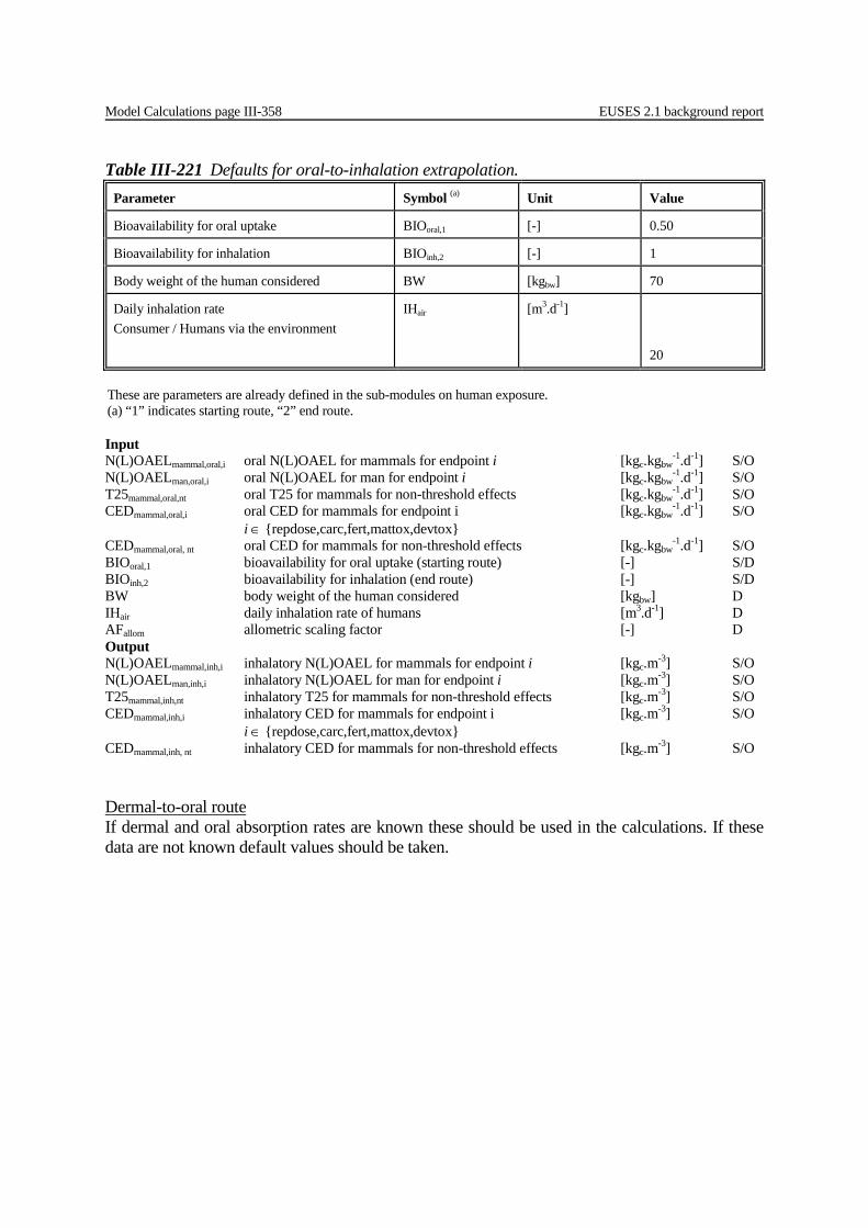
Model Calculations page III-358 EUSES 2.1 background report
Input N(L)OAELmammal,oral,i oral N(L)OAEL for mammals for endpoint i [kgc.kgbw
-1.d-1] S/O N(L)OAELman,oral,i oral N(L)OAEL for man for endpoint i [kgc.kgbw
-1.d-1] S/O T25mammal,oral,nt oral T25 for mammals for non-threshold effects [kgc.kgbw
-1.d-1] S/O CEDmammal,oral,i oral CED for mammals for endpoint i [kgc.kgbw
-1.d-1] S/O i ∈ {repdose,carc,fert,mattox,devtox} CEDmammal,oral, nt oral CED for mammals for non-threshold effects [kgc.kgbw
-1.d-1] S/O BIOoral,1 bioavailability for oral uptake (starting route) [-] S/D BIOinh,2 bioavailability for inhalation (end route) [-] S/D BW body weight of the human considered [kgbw] D IHair daily inhalation rate of humans [m3.d-1] D AFallom allometric scaling factor [-] D Output N(L)OAELmammal,inh,i inhalatory N(L)OAEL for mammals for endpoint i [kgc.m-3] S/O N(L)OAELman,inh,i inhalatory N(L)OAEL for man for endpoint i [kgc.m-3] S/O T25mammal,inh,nt inhalatory T25 for mammals for non-threshold effects [kgc.m-3] S/O CEDmammal,inh,i inhalatory CED for mammals for endpoint i [kgc.m-3] S/O i ∈ {repdose,carc,fert,mattox,devtox} CEDmammal,inh, nt inhalatory CED for mammals for non-threshold effects [kgc.m-3] S/O Dermal-to-oral route If dermal and oral absorption rates are known these should be used in the calculations. If these data are not known default values should be taken.
Table III-221 Defaults for oral-to-inhalation extrapolation. Parameter Symbol (a) Unit Value
Bioavailability for oral uptake BIOoral,1 [-] 0.50
Bioavailability for inhalation BIOinh,2 [-] 1
Body weight of the human considered BW [kgbw] 70
Daily inhalation rate Consumer / Humans via the environment
IHair [m3.d-1]
20
These are parameters are already defined in the sub-modules on human exposure. (a) “1” indicates starting route, “2” end route.

EUSES 2.1 background report Model Calculations page III-359
Table III-222 Defaults for dermal-to-oral extrapolation. Parameter Symbol (a) Unit Value
Bioavailability for dermal uptake
MOLW >500 and [log Kow <-1 or >4] MOLW ≤500 and [log Kow ≥-1 and ≤4]
BIOder,1 [-]
0.01 0.1
Bioavailability for oral uptake BIOoral,2 [-] 1 These are parameters are already defined in the sub-modules on human exposure. (a) “1” indicates starting route, “2” end route.
BIOBIO NOAEL= NOAEL
oral
derider,mammal,ioral,mammal,
2,
1,⋅ (805)
BIOBIO LOAEL= LOAEL
oral
derider,mammal,ioral,mammal,
2,
1,⋅ (806)
BIOBIO NOAEL= NOAEL
oral
derider,man,ioral,man,
2,
1,⋅ (807)
BIOBIO LOAEL= LOAEL
oral
derider,man,ioral,man,
2,
1,⋅ (808)
BIOBIO CED= CED
oral
deridermammal,ioralmammal
2,
1,,,, ⋅ (809)
devtox}mattoxfertcarc{repdose i ,,,,∈
BIOBIO T= T
oral
derntdermammalntoralmammal
2,
1,,,,, 2525 ⋅ (810)
BIOBIO CED= CED
oral
derntdermammal,ntoralmammal
2,
1,,,, ⋅ (811)
If absorption rates of humans and experimental animals differ and are known, the toxicity parameter estimated by EUSES should be corrected manually by multiplication with a factor BIOoral-animal/BIOoral-human.

Model Calculations page III-360 EUSES 2.1 background report
Input N(L)OAELmammal,der,i dermal N(L)OAEL for mammals for endpoint i [kgc.kgbw
-1.d-1] S/O N(L)OAELman,der,i dermal N(L)OAEL for man for endpoint i [kgc.kgbw
-1.d-1] S/O T25mammal,der,nt dermal T25 for mammals for non-threshold effects [kgc.kgbw
-1.d-1] S/O CEDmammal,der,i dermal CED for mammals for endpoint i [kgc.kgbw
-1.d-1] S/O i ∈ {repdose,carc,fert,mattox,devtox} CEDmammal,der, nt dermal CED for mammals for non-threshold effects [kgc.kgbw
-1.d-1] S/O BIOder,1 bioavailability for dermal uptake (starting route) [-] S/D BIOoral,2 bioavailability for oral uptake (end route) [-] S/D Output N(L)OAELmammal,oral,i oral N(L)OAEL for mammals for endpoint i [kgc.kgbw
-1.d-1] S/O N(L)OAELman,oral,i oral N(L)OAEL for man for endpoint i [kgc.kgbw
-1.d-1] S/O T25mammal,oral,nt oral T25 for mammals for non-threshold effects [kgc.kgbw
-1.d-1] S/O CEDmammal,oral,i oral CED for mammals for endpoint i [kgc.kgbw
-1.d-1] S/O i ∈ {repdose,carc,fert,mattox,devtox} CEDmammal,oral, nt oral CED for mammals for non-threshold effects [kgc.kgbw
-1.d-1] S/O Dermal-to-inhalatory route If dermal and inhalation absorption rates are known these should be used in the calculations. If these data are not known default values should be taken. The respiratory rate used has to fulfill the requirements of allometric scaling and therefore the inhalatory rate (of humans) is multiplied with the allometric correction factor (AFallom). The TGD proposes the following values: rat 4, mice 7, guinea pig 3, rabbit 2.4, monkey 2, dog 1.4.
Table III-223 Defaults for dermal-to-inhalation extrapolation. Parameter Symbol (a) Unit Value
Bioavailability for dermal uptake
MOLW >500 and [log Kow <-1 or >4] MOLW ≤500 and [log Kow ≥-1 and ≤4]
BIOder,1 [-]
0.01 0.1
Bioavailability for inhalation BIOinh,2 [-] 1
Body weight of the human considered BW [kgbw] 70
Daily inhalation rate Consumer / Humans via the environment
IHair [m3.d-1]
20
These are parameters are already defined in the sub-modules on human exposure. (a) “1” indicates starting route, “2” end route.

EUSES 2.1 background report Model Calculations page III-361
BIO
BIO
AFIHBW NOAEL= NOAEL
inh
der
allomairider,mammal,iinh,mammal,
2,
1,
.⋅⋅ (812)
BIO
BIO
AFIHBW LOAEL= LOAEL
inh
der
allomairider,mammal,iinh,mammal,
2,
1,
.⋅⋅ (813)
BIO
BIO
AFIHBW NOAEL= NOAEL
inh
der
allomairider,man,iinh,man,
2,
1,
.⋅⋅ (814)
BIO
BIO
AFIHBW LOAEL= LOAEL
inh
der
allomairider,man,iinh,man,
2,
1,
.⋅⋅ (815)
BIOBIO
AFIHBW CED= CED
inh
der
allomairidermammal,iinhmammal
2,
1,,,, .
⋅⋅ (816)
devtox}mattoxfertcarc{repdose i ,,,,∈
BIOBIO
AFIHBW T= T
inh
der
allomairntdermammalntinhmammal
2,
1,,,,, .
2525 ⋅⋅ (817)
BIOBIO
AFIHBW CED= CED
inh
der
allomairntdermammal,ntinhmammal
2,
1,,,, .
⋅⋅ (818)
If absorption rates of humans and experimental animals differ and are known, the toxicity parameter estimated by EUSES should be corrected manually by multiplication with a factor BIOinh-animal/BIOinh-human.
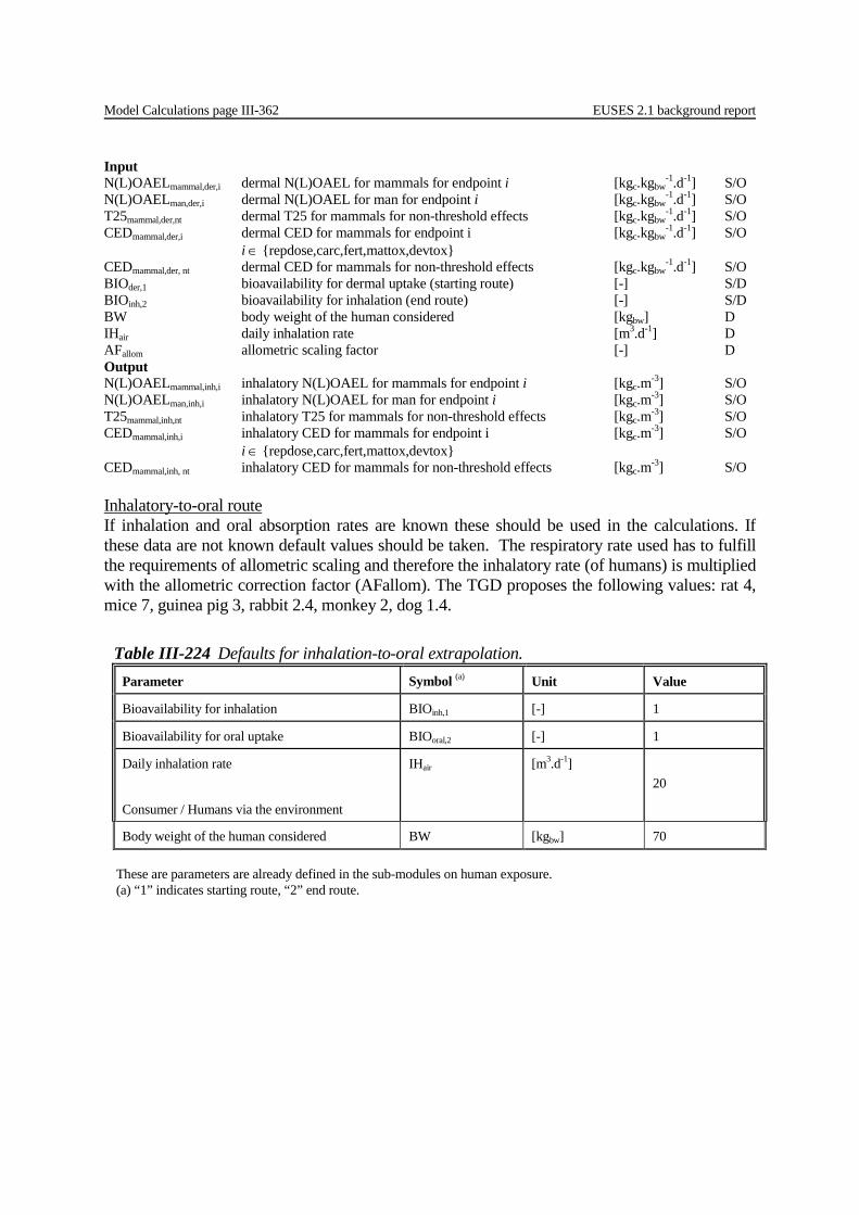
Model Calculations page III-362 EUSES 2.1 background report
Input N(L)OAELmammal,der,i dermal N(L)OAEL for mammals for endpoint i [kgc.kgbw
-1.d-1] S/O N(L)OAELman,der,i dermal N(L)OAEL for man for endpoint i [kgc.kgbw
-1.d-1] S/O T25mammal,der,nt dermal T25 for mammals for non-threshold effects [kgc.kgbw
-1.d-1] S/O CEDmammal,der,i dermal CED for mammals for endpoint i [kgc.kgbw
-1.d-1] S/O i ∈ {repdose,carc,fert,mattox,devtox} CEDmammal,der, nt dermal CED for mammals for non-threshold effects [kgc.kgbw
-1.d-1] S/O BIOder,1 bioavailability for dermal uptake (starting route) [-] S/D BIOinh,2 bioavailability for inhalation (end route) [-] S/D BW body weight of the human considered [kgbw] D IHair daily inhalation rate [m3.d-1] D AFallom allometric scaling factor [-] D Output N(L)OAELmammal,inh,i inhalatory N(L)OAEL for mammals for endpoint i [kgc.m-3] S/O N(L)OAELman,inh,i inhalatory N(L)OAEL for man for endpoint i [kgc.m-3] S/O T25mammal,inh,nt inhalatory T25 for mammals for non-threshold effects [kgc.m-3] S/O CEDmammal,inh,i inhalatory CED for mammals for endpoint i [kgc.m-3] S/O i ∈ {repdose,carc,fert,mattox,devtox} CEDmammal,inh, nt inhalatory CED for mammals for non-threshold effects [kgc.m-3] S/O Inhalatory-to-oral route If inhalation and oral absorption rates are known these should be used in the calculations. If these data are not known default values should be taken. The respiratory rate used has to fulfill the requirements of allometric scaling and therefore the inhalatory rate (of humans) is multiplied with the allometric correction factor (AFallom). The TGD proposes the following values: rat 4, mice 7, guinea pig 3, rabbit 2.4, monkey 2, dog 1.4.
Table III-224 Defaults for inhalation-to-oral extrapolation. Parameter Symbol (a) Unit Value
Bioavailability for inhalation BIOinh,1 [-] 1
Bioavailability for oral uptake BIOoral,2 [-] 1
Daily inhalation rate
Consumer / Humans via the environment
IHair [m3.d-1] 20
Body weight of the human considered BW [kgbw] 70 These are parameters are already defined in the sub-modules on human exposure. (a) “1” indicates starting route, “2” end route.
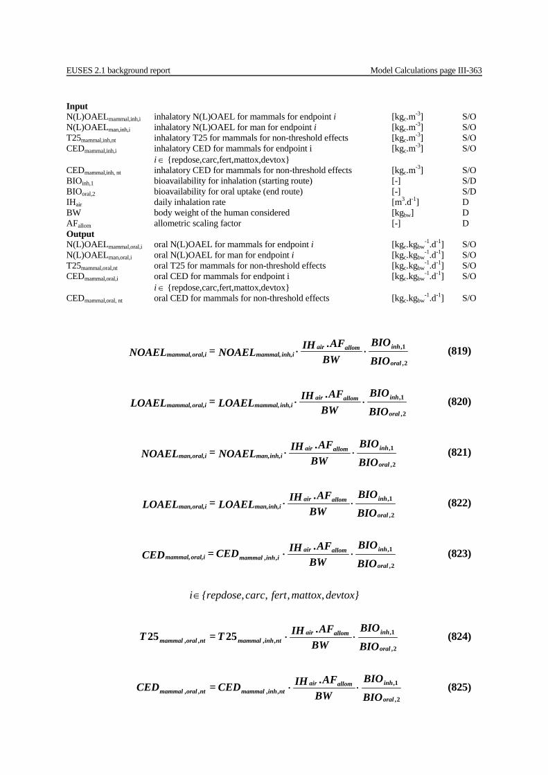
EUSES 2.1 background report Model Calculations page III-363
Input N(L)OAELmammal,inh,i inhalatory N(L)OAEL for mammals for endpoint i [kgc.m-3] S/O N(L)OAELman,inh,i inhalatory N(L)OAEL for man for endpoint i [kgc.m-3] S/O T25mammal,inh,nt inhalatory T25 for mammals for non-threshold effects [kgc.m-3] S/O CEDmammal,inh,i inhalatory CED for mammals for endpoint i [kgc.m-3] S/O i ∈ {repdose,carc,fert,mattox,devtox} CEDmammal,inh, nt inhalatory CED for mammals for non-threshold effects [kgc.m-3] S/O BIOinh,1 bioavailability for inhalation (starting route) [-] S/D BIOoral,2 bioavailability for oral uptake (end route) [-] S/D IHair daily inhalation rate [m3.d-1] D BW body weight of the human considered [kgbw] D AFallom allometric scaling factor [-] D Output N(L)OAELmammal,oral,i oral N(L)OAEL for mammals for endpoint i [kgc.kgbw
-1.d-1] S/O N(L)OAELman,oral,i oral N(L)OAEL for man for endpoint i [kgc.kgbw
-1.d-1] S/O T25mammal,oral,nt oral T25 for mammals for non-threshold effects [kgc.kgbw
-1.d-1] S/O CEDmammal,oral,i oral CED for mammals for endpoint i [kgc.kgbw
-1.d-1] S/O i ∈ {repdose,carc,fert,mattox,devtox} CEDmammal,oral, nt oral CED for mammals for non-threshold effects [kgc.kgbw
-1.d-1] S/O
BIO
BIO
BWAFIH NOAEL= NOAEL
oral
inhallomairiinh,mammal,ioral,mammal,
2,
1,.⋅⋅ (819)
BIO
BIO
BWAFIH LOAEL= LOAEL
oral
inhallomairiinh,mammal,ioral,mammal,
2,
1,.⋅⋅ (820)
BIO
BIO
BWAFIH NOAEL= NOAEL
oral
inhallomairiinh,man,ioral,man,
2,
1,.⋅⋅ (821)
BIO
BIO
BWAFIH LOAEL= LOAEL
oral
inhallomairiinh,man,ioral,man,
2,
1,.⋅⋅ (822)
BIO
BIO
BWAFIH CED= CED
oral
inhallomairiinhmammalioral,mammal,
2,
1,,,
.⋅⋅ (823)
devtox}mattoxfertcarc{repdose i ,,,,∈
BIO
BIO
BWAFIH T= T
oral
inhallomairntinhmammalntoralmammal
2,
1,,,,,
.2525 ⋅⋅ (824)
BIO
BIO
BWAFIH CED= CED
oral
inhallomairntinhmammalntoralmammal
2,
1,,,,,
.⋅⋅ (825)
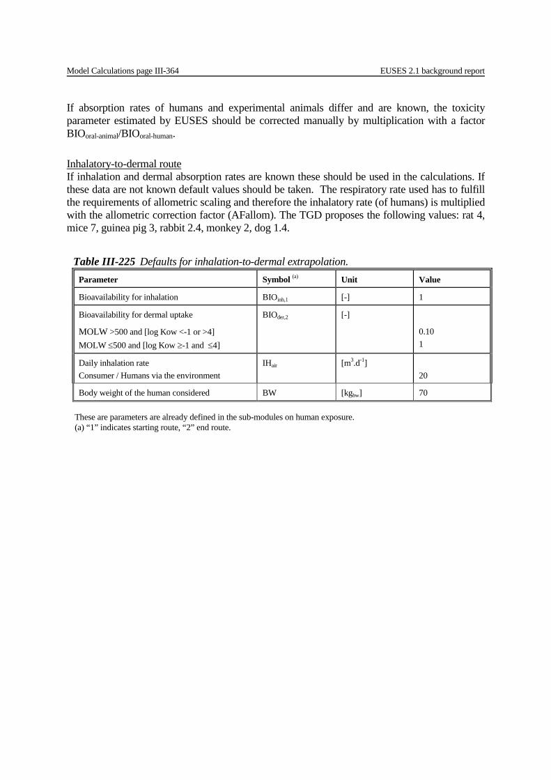
Model Calculations page III-364 EUSES 2.1 background report
If absorption rates of humans and experimental animals differ and are known, the toxicity parameter estimated by EUSES should be corrected manually by multiplication with a factor BIOoral-animal/BIOoral-human.
Inhalatory-to-dermal route If inhalation and dermal absorption rates are known these should be used in the calculations. If these data are not known default values should be taken. The respiratory rate used has to fulfill the requirements of allometric scaling and therefore the inhalatory rate (of humans) is multiplied with the allometric correction factor (AFallom). The TGD proposes the following values: rat 4, mice 7, guinea pig 3, rabbit 2.4, monkey 2, dog 1.4.
Table III-225 Defaults for inhalation-to-dermal extrapolation. Parameter Symbol (a) Unit Value
Bioavailability for inhalation BIOinh,1 [-] 1
Bioavailability for dermal uptake
MOLW >500 and [log Kow <-1 or >4] MOLW ≤500 and [log Kow ≥-1 and ≤4]
BIOder,2 [-]
0.10 1
Daily inhalation rate Consumer / Humans via the environment
IHair [m3.d-1] 20
Body weight of the human considered BW [kgbw] 70 These are parameters are already defined in the sub-modules on human exposure. (a) “1” indicates starting route, “2” end route.
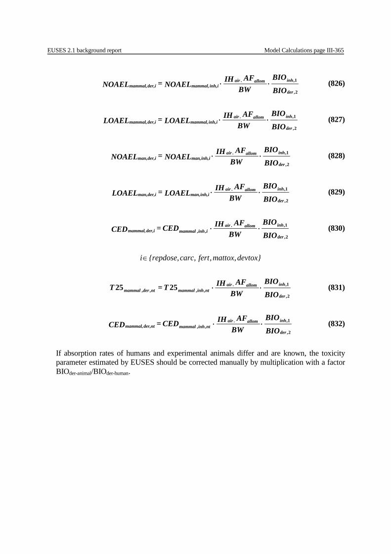
EUSES 2.1 background report Model Calculations page III-365
BIO
BIO
BWAFIH NOAEL= NOAEL
der
inhallomairiinh,mammal,ider,mammal,
2,
1,. ⋅⋅ (826)
BIO
BIO
BWAFIH LOAEL= LOAEL
der
inhallomairiinh,mammal,ider,mammal,
2,
1,. ⋅⋅ (827)
BIO
BIO
BWAFIH NOAEL= NOAEL
der
inhallomairiinh,man,ider,man,
2,
1,. ⋅⋅ (828)
BIO
BIO
BWAFIH LOAEL= LOAEL
der
inhallomairiinh,man,ider,man,
2,
1,. ⋅⋅ (829)
BIO
BIO
BWAFIH CED= CED
der
inhallomairiinhmammalider,mammal,
2,
1,.,, ⋅⋅ (830)
devtox}mattoxfertcarc{repdose i ,,,,∈
BIO
BIO
BWAFIH T= T
der
inhallomairntinhmammalntdermammal
2,
1,.,,,, 2525 ⋅⋅ (831)
BIO
BIO
BWAFIH CED= CED
der
inhallomairntinhmammalntder,mammal,
2,
1,.,, ⋅⋅ (832)
If absorption rates of humans and experimental animals differ and are known, the toxicity parameter estimated by EUSES should be corrected manually by multiplication with a factor BIOder-animal/BIOder-human.
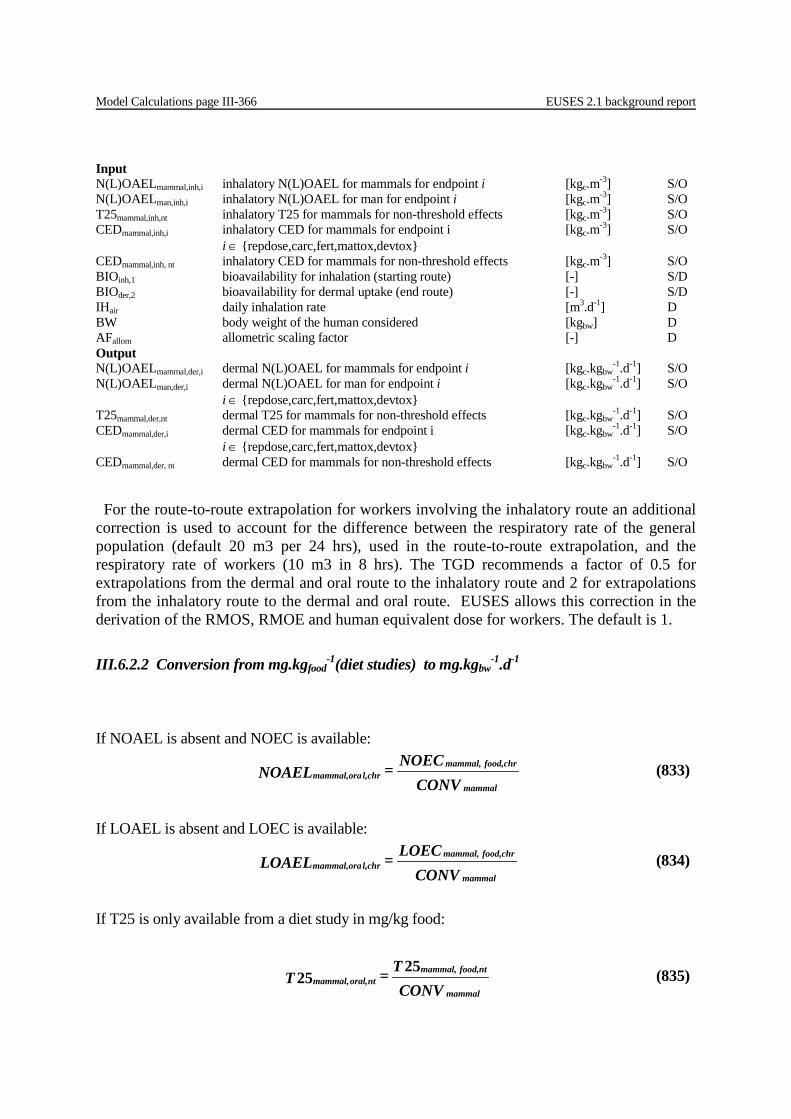
Model Calculations page III-366 EUSES 2.1 background report
Input N(L)OAELmammal,inh,i inhalatory N(L)OAEL for mammals for endpoint i [kgc.m-3] S/O N(L)OAELman,inh,i inhalatory N(L)OAEL for man for endpoint i [kgc.m-3] S/O T25mammal,inh,nt inhalatory T25 for mammals for non-threshold effects [kgc.m-3] S/O CEDmammal,inh,i inhalatory CED for mammals for endpoint i [kgc.m-3] S/O i ∈ {repdose,carc,fert,mattox,devtox} CEDmammal,inh, nt inhalatory CED for mammals for non-threshold effects [kgc.m-3] S/O BIOinh,1 bioavailability for inhalation (starting route) [-] S/D BIOder,2 bioavailability for dermal uptake (end route) [-] S/D IHair daily inhalation rate [m3.d-1] D BW body weight of the human considered [kgbw] D AFallom allometric scaling factor [-] D Output N(L)OAELmammal,der,i dermal N(L)OAEL for mammals for endpoint i [kgc.kgbw
-1.d-1] S/O N(L)OAELman,der,i dermal N(L)OAEL for man for endpoint i [kgc.kgbw
-1.d-1] S/O i ∈ {repdose,carc,fert,mattox,devtox} T25mammal,der,nt dermal T25 for mammals for non-threshold effects [kgc.kgbw
-1.d-1] S/O CEDmammal,der,i dermal CED for mammals for endpoint i [kgc.kgbw
-1.d-1] S/O i ∈ {repdose,carc,fert,mattox,devtox} CEDmammal,der, nt dermal CED for mammals for non-threshold effects [kgc.kgbw
-1.d-1] S/O For the route-to-route extrapolation for workers involving the inhalatory route an additional correction is used to account for the difference between the respiratory rate of the general population (default 20 m3 per 24 hrs), used in the route-to-route extrapolation, and the respiratory rate of workers (10 m3 in 8 hrs). The TGD recommends a factor of 0.5 for extrapolations from the dermal and oral route to the inhalatory route and 2 for extrapolations from the inhalatory route to the dermal and oral route. EUSES allows this correction in the derivation of the RMOS, RMOE and human equivalent dose for workers. The default is 1.
III.6.2.2 Conversion from mg.kgfood-1(diet studies) to mg.kgbw
-1.d-1
If NOAEL is absent and NOEC is available:
CONV
NOEC= NOAELmammal
food,chrmammal,l,chrmammal,ora (833)
If LOAEL is absent and LOEC is available:
CONV
LOEC= LOAELmammal
food,chrmammal,l,chrmammal,ora (834)
If T25 is only available from a diet study in mg/kg food:
CONV
T= Tmammal
ntfood,mammal,ntoral,mammal,
2525 (835)
EUSES 2.1 background report Model Calculations page III-367
If CED is only available from a diet study in mg/kg food:
CONV
CED= CEDmammal
ntfood,mammal,ntoral,mammal, (836)
devtox}mattoxfertcarc{repdose i ,,,,∈
Input N(L)OECmammal,food,i N(L)OEC via food for mammals for endpoint i [kgc.kgfood
-1] S/O T25mammal,food,nt T25 via food for mammals for non-threshold substances [kgc.kgfood
-1] S/O CEDmammal,food,i CED via food for mammals for endpoint i [kgc.kgfood
-1] S/O CEDmammal,food,nt CED via food for mammals for non-threshold substances [kgc.kgfood
-1] S/O CONVmammal conversion factor NOAEL to NOEC [kgbw.d.kgfood
-1] P/S a i ∈ {repdose,carc,fert,mattox,devtox} Output N(L)OAELmammal,oral,i oral N(L)OAEL for mammals for endpoint i [kgc.kgbw
-1.d-1] S/O T25mammal,oral,nt oral T25 for mammals for non-threshold effects [kgc.kgbw
-1.d-1] S/O CEDmammal,oral,i oral CED for mammals for endpoint i [kgc.kgbw
-1.d-1] S/O i ∈ {repdose,carc,fert,mattox,devtox} CEDmammal,oral, nt oral CED for mammals for non-threshold effects [kgc.kgbw
-1.d-1] S/O a see Table III-219 in Section III.6.1.5.
Model Calculations page III-368 EUSES 2.1 background report
III.7 RISK CHARACTERISATION In risk characterisation, exposure levels are compared to suitable no-effect levels to yield so-called Risk Characterisation Ratios (RCR) for each protection goal. For the environmental end-points, this is the ratio of PEC to PNEC. For the human end-points a distinction need to be made between threshold and non-threshold substances. For threshold substances the Margin Of Safety (MOS) is derived, i.e. the ratio of the effect parameter and the estimated exposure value. The MOS is compared to a reference-MOS. In addition, for biocides the Acceptable-Operator-Exposure-Level (AOEL) is compared to the internal exposure value. Risk characterisation of non-threshold substances entails a comparison between the estimated exposure and the T25 or BMD05, extrapolated to a lifetime cancer risk for humans. Additionally, the Margin of Exposure (MOE) approach is followed. This approach is equivalent to the MOS approach for threshold substances: the MOE is the ratio of the effect parameter (T25 or BMD05) and the estimated lifetime daily exposure level. The MOE is to be compared to the reference-MOE.. Environmental risk characterisation and human health risk characterisation are handled in separate sub-modules. This module is divided into four specific sub-modules, which will be treated separately: • Environment. • Indirect human exposure. • Consumer exposure. • Workplace exposure.

EUSES 2.1 background report Model Calculations page III-369
III.7.1 Risk characterisation for the environment Input PEClocalwater local PEC in surface water during emission episode [kgc.m-3] PEClocalwater,marine local PEC in marine surface water during emission episode [kgc.m-3] PECregwater regional steady-state PEC in surface water [kgc.m-3] PECregwater,marine regional steady-state PEC in marine surface water [kgc.m-3] PNECwater PNEC for the aquatic compartment [kgc.m-3] c PNECwater,marine PNEC for the marine aquatic compartment [kgc.m-3] c PEClocalsoil local PEC in agricultural soil, averaged over 30 days [kgc.kgwwt
-1] PECregagric regional steady-state PEC in agricultural soil [kgc.kgwwt
-1] PNECsoil PNEC for the soil compartment [kgc.kgwwt
-1] c TOXterr toxicological data used for extrapolation of PNEC [kgc.kgwwt
-1] EPterr equilibrium partitioning used for PNEC for soil? [yes/no] c Kow octanol-water partition coefficient [m3.m-3] PEClocalsed local PEC in sediment [kgc.kgwwt
-1] PEClocalsed,marine local PEC in marine sediment [kgc.kgwwt
-1] PECregsed regional steady-state PEC in sediment [kgc.kgwwt
-1] PECregsed,marine regional steady-state PEC in marine sediment [kgc.kgwwt
-1] PNECsed PNEC for the sediment compartment [kgc.kgwwt
-1] PNECsed,marine PNEC for the marine sediment compartment [kgc.kgwwt
-1] EPsed equilibrium partitioning used for PNEC for sediment? [yes/no] c EPsedmarine equilibrium partitioning used for PNEC for marine sediment? [yes/no] c PECstp local PEC in STP during emission episode [kgc.m-3] PNECmicro-organisms PNEC for STP micro-organisms [kgc.m-3] c PECoral,fish PEC in fish (local and regional combined) [kgc.kgwwt
-1] PECoral,fish,marine PEC in marine fish (local and regional combined) [kgc.kgwwt
-1] PECoral,fish predator,marine PEC in marine fish-eating predator (local and regional combined) [kgc.kgwwt
-1] PECoral,worm PEC in worm (local and regional combined) [kgc.kgwwt
-1] PNECoral PNEC for birds and mammals [kgc.kgwwt
-1] c PNECstatwater PNEC for aquatic organisms with statistical method [kgc.m-3] PNECstatwater, marine PNEC for marine aquatic organisms with statistical method [kgc.m-3] PNECstatsoil PNEC for terrestrial organisms with statistical method [kgc.m-3] Output RCRlocalwater RCR for the local water compartment [-] c RCRlocalwater,marine RCR for the local marine water compartment [-] c RCRregwater RCR for the regional water compartment [-] c RCRregwater,marine RCR for the regional marine water compartment [-] c RCRlocalsoil RCR for the local soil compartment [-] c RCRregsoil RCR for the regional soil compartment [-] c RCRlocalsed RCR for the local sediment compartment [-] c RCRlocalsed,marine RCR for the local marine sediment compartment [-] c RCRregsed RCR for the regional sediment compartment [-] c RCRregsed,marine RCR for the regional marine sediment compartment [-] c RCRstp RCR for the sewage treatment plant [-] c RCRoral,fish RCR for fish-eating birds and mammals [-] c RCRoral,fish,marine RCR for fish-eating birds/mammals (marine environment) [-] c RCRoral,fish predator,marine RCR for top-predators (marine environment) [-] c RCRoral,worm RCR for worm-eating birds and mammals [-] c RCRstatwater RCR for aquatic organisms with statistical method [-] c RCRstatwater, marine RCR for marine aquatic organisms with statistical method [-] c RCRstatsoil RCR for terrestrial organisms with statistical method [-] c

Model Calculations page III-370 EUSES 2.1 background report
III.7.1.1 Aquatic environment The concentration of the chemical in surface water is compared to the no-effect concentration for aquatic organisms. This is done for the local as well as the regional freshwater and marine environment. On the local scale, the concentration during an emission episode is taken. It should be noted that the local ratios have to be defined for all relevant stages of the life cycle and for each application of the substance.
Input PEClocalwater local PEC in surface water during emission episode [kgc.m-3] O PECregwater regional steady-state PEC in surface water [kgc.m-3] O PEClocalwater,marine local PEC in marine water during emission episode [kgc.m-3] O PECregwater,marine regional steady-state PEC in marine surface water [kgc.m-3] O PNECwater PNEC for aquatic compartment [kgc.m-3] Oc PNECwater,marine PNEC for marine aquatic compartment [kgc.m-3] Oc Output RCRlocalwater RCR for local water compartment [-] Oc RCRregwater RCR for regional water compartment [-] Oc RCRlocalwater,marine RCR for local marine water compartment [-] Oc RCRregwater,marine RCR for regional marine water compartment [-] Oc
PNEC
PEClocal= RCRlocalwater
waterwater (837)
PNEC
PEClocal= RCRlocalmarinewater
marinewatermarinewater
,
,, (838)
PNEC
PECreg= RCRregwater
waterwater (839)
PNEC
PECreg= RCRreg
marinewater
marinewatermarinewater
,
,, (840)

EUSES 2.1 background report Model Calculations page III-371
III.7.1.2 Terrestrial compartment The concentration of the chemical in agricultural soil is compared to the no-effect concentration for terrestrial organisms. This is done for the local as well as the regional environment. On the local scale, the concentration averaged over 30 days is used. It should be noted that the local ratios have to be defined for all relevant stages of the life cycle and for each application of the substance. For substances with a log Kow greater than 5, the equilibrium-partitioning method is used in a modified way. For these substances, the PEC/PNEC in soil is increased by a factor of 10 to account for uptake via ingestion of soil.
PNEC
PEClocal= RCRlocalsoil
soilsoil (841)
PNEC
PECreg= RCRreg
soil
agricsoil (842)
If EPterr = yes and log Kow > 5 then
If EPterr = yes and log Kow > 5 then
10⋅
PNEC
PECreg= RCRreg
soil
agricsoil
(844)
Input PEClocalsoil local PEC in agricultural soil, averaged over 30 days [kgc.kgwwt
-1] O PECregagric regional steady-state PEC in agricultural soil [kgc.kgwwt
-1] O PNECsoil PNEC for soil compartment [kgc.kgwwt
-1] Oc EPterr equilibrium partitioning used for PNEC? [yes/no] Oc Kow octanol-water partition coefficient [m3.m-3] S Output RCRlocalsoil RCR for local soil compartment [-] Oc RCRregsoil RCR for regional soil compartment [-] Oc
10⋅
PNECPEClocal= RCRlocal
soil
soilsoil
(843)
Model Calculations page III-372 EUSES 2.1 background report
III.7.1.3 Sediment compartment The concentration of the chemical in sediment is compared to the no-effect concentration for sediment-dwelling organisms. This is done for the local as well as the regional freshwater and marine environment. It should be noted that the local ratios have to be defined for all relevant stages of the life cycle and for each application of the substance. For substances with a log Kow greater than 5, the equilibrium-partitioning method is used in a modified way. For these substances, the PEC/PNEC in sediment is increased by a factor of 10 to account for uptake via ingestion of sediment. It should be noted that a risk characterisation for sediment is only feasible if measured data are used to overwrite the estimates for PEC and/or PNEC in sediment (otherwise, equilibrium partitioning is applied to derive both PEC and PNEC).
PNEC
PEClocal= RCRlocalsed
sedsed (845)
PNEC
PEClocal= RCRlocalmarinesed
marinesedmarinesed
,
,, (846)
PNEC
PECreg= RCRreg
sed
sedsed (847)
PNEC
PECreg= RCRreg
marinesed
marinesedmarinesed
,
,, (848)
If EPsed = yes and log Kow > 5 then:
10⋅PNEC
PEClocal= RCRlocalsed
sedsed (849)
10⋅PNEC
PECreg= RCRreg
sed
sedsed (850)
If EPsedmarine = yes and log Kow > 5 then:
10,
,, ⋅
PNECPEClocal= RCRlocal
marinesed
marinesedmarinesed (851)
10,
,, ⋅
PNEC
PECreg= RCRreg
marinesed
marinesedmarinesed (852)

EUSES 2.1 background report Model Calculations page III-373
Input PEClocalsed local PEC in sediment [kgc.kgwwt
-1] O PEClocalsed,marine local PEC in marine sediment [kgc.kgwwt
-1] O PECregsed regional steady-state PEC in sediment [kgc.kgwwt
-1] O PECregsed,marine regional steady-state PEC in marien sediment [kgc.kgwwt
-1] O PNECsed PNEC for the sediment compartment [kgc.kgwwt
-1] O PNECsed,marine PNEC for the marine sediment compartment [kgc.kgwwt
-1] O EPsed equilibrium partitioning used for PNEC for sediment? [yes/no] Oc EPsedmarine equilibrium partitioning used for PNEC for marine sediment? [yes/no] Oc Kow octanol-water partition coefficient [m3.m-3] S Output RCRlocalsed RCR for local sediment compartment [-] Oc RCRlocalsed,marine RCR for local marine sediment compartment [-] Oc RCRregsed RCR for regional sediment compartment [-] Oc RCRregsed,marine RCR for regional marine sediment compartment [-] Oc
III.7.1.4 Micro-organisms in STP The concentration of the chemical in the sewage treatment plant is compared to the no-effect concentration for micro-organisms. This is done for the local environment only. The concentration during an emission episode is used. It should be noted that the ratios have to be defined for all relevant stages of the life cycle and for each application of the substance.
Input PECstp local PEC in STP during emission episode [kgc.m-3] O PNECmicro-organisms PNEC for STP micro-organisms [kgc.m-3] Oc Output RCRstp RCR for sewage treatment plant [-] Oc
III.7.1.5 Predators in freshwater and marine environment The concentration of the chemical in fish and in fish-eating predator is compared to the no-effect concentration for birds and mammals. Local and regional concentrations are combined for calculating the concentration in fish and fish-eating predator . It should be noted that the ratios have to be defined for all relevant stages of the life cycle and for each application of the substance.
PNEC
PEC= RCRorganisms-micro
stpstp (853)
PNECPEC= RCR
oral
fishoral,fishoral, (854)
PNEC
PEC= RCRoral
marinefishoral,marinefishoral,
,, (855)
Model Calculations page III-374 EUSES 2.1 background report
PNEC
PEC= RCRoral
marinepredatorfishoral,marinepredatorfishoral,
,, (856)
put PECoral,fish PEC in fish (local and regional combined) [kgc.kgwwt
-1] O PECoral,fish,marine PEC in marine fish (local and regional combined) [kgc.kgwwt
-1] O PECoral,fish predator,marine PEC in marine fish-eating predator (local and regional combined) [kgc.kgwwt
-1] O PNECoral PNEC for birds and mammals [kgc.kgwwt
-1] Oc Output RCRoral,fish RCR for fish-eating birds/mammals (freshwater environment) [-] Oc RCRoral,fish,marine RCR for fish-eating birds/mammals (marine environment) [-] Oc RCRoral,fish predator,marine RCR for top-predators (marine environment) [-] Oc
III.7.1.6 Worm-eating predators The concentration of the chemical in earthworms is compared to the no-effect concentration for birds and mammals. There is only one concentration in earthworms as local and regional are combined in this concentration. It should be noted that the ratios have to be defined for all relevant stages of the life cycle and for each application of the substance.
PNEC
PEC= RCRoral
wormoral,wormoral, (857)
Input PECoral,worm PEC in worm (local and regional combined) [kgc.kgwwt
-1] O PNECoral PNEC for birds and mammals [kgc.kgwwt
-1] Oc Output RCRoral,worm RCR for worm-eating birds and mammals [-] Oc

EUSES 2.1 background report Model Calculations page III-375
III.7.2 Risk characterisation for human health For threshold-based effects, the quantitative risk characterisation is carried out by calculating 'Margins Of Safety' (MOS) and comparing this to a reference-MOS (MOS approach). This MOS approach is not applicable for non-threshold based effects. Next to the MOS approach, for biocides an Acceptable Operator Exposure Level (AOEL) is to be derived, which should be compared to the estimated exposure values. For non-threshold effects, i.e. genotoxic carcinogens, lifetime cancer risk is calculated based on T25 or CED05. Additionally, the Margin of Exposure (MOE) is calculated and compared to a reference-MOE (RMOE).
a Correction for differences in metabolic size: the TGD recommends 4 for rats, 7 for mice, 3 for guinea pigs, 2.4 for rabbits, 2 for monkeys and 1.4 for dogs b The TGD recommends 2.5 c The TGD recommends 5 for workers and 10 for the general population dThe TGD recommends 3 for subacute to sub/semi-chronic extrapolation, 2 for sub/semi-chronic to chronic extrapolation amd 6 for subacute to chronic extrapolation e Factor to account for uncertainty in the route-to-route extrapolation f Factor to account for uncertainty in the dose-response extrapolation; includes uncertainty regarding the nature of the effect and the quality of the database g Factor, used for the calculation of the reference-MOE for non-threshold substances, accounting for the extrapolation for the high risk related to the T25 (25:100) to a low reference level, default chosen to be 1:106
h Factor accounting for the difference between the respiratory rate of the general population (default 20 m3 per 24 hrs) used in the route-to-route extrapolation and the respiratory rate of workers (10 m3 in 8 hrs). The TGD recommends a factor of 0.5 for extrapolations from the dermal and oral route to the inhalatory route and 2 for extrapolations from the inhalatory route to the dermal and oral route.
Table III-226 Defaults factors Assessment factor Symbol Unit Value
Allometric scaling factor AFallom [-] 1a
Remaining interspecies differences AFinter [-] 1b
Intraspecies differences AFintra [-] 1c
Differences in exposure duration AFexpdur [-] 1d
Differences in exposure route AFexprt [-] 1e
Dose-response relationship AFdose-resp [-] 1f
Low risk extrapolation factor AFlr [-] 250,000g
Correction factors workers
Correction factor for route-to route extrapolation to account for difference in ventilation rate between workers and general population
CFoccup1 [-] 1h
Correction factor for duration and frequency of exposure
CFoccup2 [-] 2.8
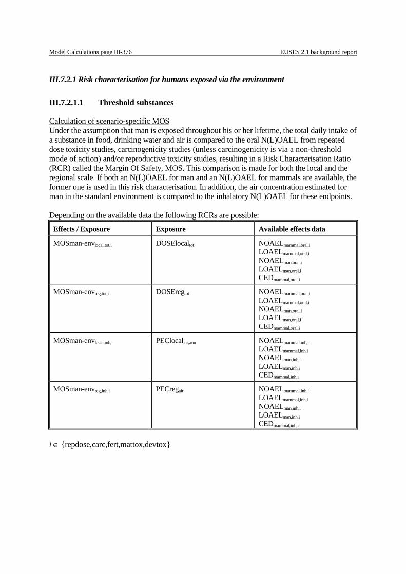
Model Calculations page III-376 EUSES 2.1 background report
III.7.2.1 Risk characterisation for humans exposed via the environment III.7.2.1.1 Threshold substances Calculation of scenario-specific MOS Under the assumption that man is exposed throughout his or her lifetime, the total daily intake of a substance in food, drinking water and air is compared to the oral N(L)OAEL from repeated dose toxicity studies, carcinogenicity studies (unless carcinogenicity is via a non-threshold mode of action) and/or reproductive toxicity studies, resulting in a Risk Characterisation Ratio (RCR) called the Margin Of Safety, MOS. This comparison is made for both the local and the regional scale. If both an N(L)OAEL for man and an N(L)OAEL for mammals are available, the former one is used in this risk characterisation. In addition, the air concentration estimated for man in the standard environment is compared to the inhalatory N(L)OAEL for these endpoints. Depending on the available data the following RCRs are possible:
Effects / Exposure Exposure Available effects data
MOSman-envlocal,tot,i DOSElocaltot NOAELmammal,oral,i LOAELmammal,oral,i NOAELman,oral,i LOAELman,oral,i CEDmammal,oral,i
MOSman-envreg,tot,i DOSEregtot NOAELmammal,oral,i LOAELmammal,oral,i NOAELman,oral,i LOAELman,oral,i CEDmammal,oral,i
MOSman-envlocal,inh,i PEClocalair,ann NOAELmammal,inh,i LOAELmammal,inh,i NOAELman,inh,i LOAELman,inh,i CEDmammal,inh,i
MOSman-envreg,inh,i PECregair NOAELmammal,inh,i LOAELmammal,inh,i NOAELman,inh,i LOAELman,inh,i CEDmammal,inh,i
i ∈ {repdose,carc,fert,mattox,devtox}

EUSES 2.1 background report Model Calculations page III-377
Input N(L)OAELmammal,oral,i oral N(L)OAEL for mammals for endpoint of concern [kgc.kgbw
-1.d-1] S/O N(L)OAELman,oral,i oral N(L)OAEL for man for endpoint of concern [kgc.kgbw
-1.d-1] S/O N(L)OAELmammal,inh,i inhalatory N(L)OAEL for mammals for endpoint of concern [kgc.m-3] S/O N(L)OAELman,inh,i inhalatory N(L)OAEL for man for endpoint of concern [kgc.m-3] S/O CEDmammal,oral,i oral CED for mammals for endpoint of concern [kgc.kgbw
-1.d-1] S CEDmammal,inh,i inhalatory CED for mammals for endpoint of concern [kgc.m-3] S DOSElocaltot local total daily intake for humans [kgc.kgbw
-1.d-1] O DOSEregtot regional total daily intake for humans [kgc.kgbw
-1.d-1] O PEClocalair,ann annual average local PEC in air (total) [kgc.m-3] O PECregair regional PEC in air (total) [kgc.m-3] O i ∈ {repdose,carc,fert,mattox,devtox} Output MOSman-envlocal,tot,i MOS local, total exposure via all media, for endpoint of concern [-] Oc MOSman-envlocal,inh,i MOS local, exposure via air, for endpoint of concern [-] Oc MOSman-envreg,tot,i MOS regional, total exposure via all media, for endpoint of conc. [-] Oc MOSman-envreg,inh,i MOS regional, exposure via air, for endpoint of concern [-] Oc i ∈ {repdose,carc,fert,mattox,devtox} Derivation of scenario-specific reference-MOS In order to account for the various uncertainties and variabilities in the extrapolation from experimental data to the human situation and in the available data set, per scenario under consideration a reference-MOS is to be derived. All aspects that can be dealt with quantitatively (as assessment factors) are combined to form the overall assessment factor or reference-MOS (RMOS).
x ∈ {local,reg} y ∈ {tot,inh} i ∈ {repdose,carc,fert,mattox,devtox} Input AFallom assessment factor for allometric scaling [-] S/D AFinter assessment factor for remaining interspecies differences [-] S/D AFintra assessment factor for intraspecies differences [-] S/D AFexpdur assessment factor for differences in exposure duration [-] S/D AFexprt assessment factor for differences in exposure route [-] S/D AFdose-resp assessment factor for dose-response relationship [-] S/D Output RMOSman-envlocal,tot,i reference-MOS local, total exposure via all media, for endpoint of concern [-] Oc RMOSman-envlocal,inh,i reference-MOS local, exposure via air, for endpoint of concern [-] Oc RMOSman-envreg,tot,i reference-MOS regional, total exposure via all media, for endpoint of concern [-] Oc RMOSman-envreg.inh,i reference-MOS regional, exposure via air, for endpoint of concern [-] Oc i ∈ {repdose,carc,fert,mattox,devtox}
AF AF AF AF AF AF= envRMOSman respdosertdurallom raeriyx −⋅⋅⋅⋅⋅− expexpintint,, (858)

Model Calculations page III-378 EUSES 2.1 background report
Comparison of MOS with reference-MOS In judging the acceptability of the MOS, in a second step of the quantitative risk characterisation the MOS is compared to the reference-MOS, resulting in a MOS/reference-MOS ratio (MRR). Depending on the available data the following MRRs are possible:
RCR / reference-MOS RCR Reference-MOS
MRRman-envlocal,tot,i MOSman-envlocal,tot,i RMOSman-envlocal,tot,i
MRRman-envreg,tot,i MOSman-envreg,tot,i RMOSman-envreg,tot,i
MRRman-envlocal,inh,i MOSman-envlocal,inh,i RMOSman-envlocal,inh,i
MRRman-envreg,inh,i MOSman-envreg,inh,i RMOSman-envreg,inh,i
i ∈ {repdose,carc,fert,mattox,devtox} Input MOSman-envlocal,tot,i MOS local, total exposure via all media, for endpoint of concern [-] Oc MOSman-envlocal,inh,i MOS local, exposure via air, for endpoint of concern [-] Oc MOSman-envreg,tot,i MOS regional, total exposure via all media, for endpoint of conc. [-] Oc MOSman-envreg,inh,i MOS regional, exposure via air, for endpoint of concern [-] Oc RMOSman-envlocal,tot,i reference-MOS local, total exposure via all media, for endpoint of concern [-] Oc RMOSman-envlocal,inh,i reference-MOS local, exposure via air, for endpoint of concern [-] Oc RMOSman-envreg,tot,i reference-MOS regional, total exposure via all media, for endpoint of concern [-] Oc RMOSman-envreg.inh,i reference-MOS regional, exposure via air, for endpoint of concern [-] Oc i ∈ {repdose,carc,fert,mattox,devtox} Output MRRman-envlocal,tot,i ratio MOS/reference-MOS local, total exposure via all media, for endp. of concern [-] Oc MRRman-envlocal,inh,i ratio MOS/reference-MOS local, exposure via air, for endpoint of concern [-] Oc MRRman-envreg,tot,i ratio MOS/reference-MOS regional, total exposure via all media, for endp. of conc. [-] Oc MRRman-envreg.inh,i ratio MOS/reference-MOS regional, exposure via air, for endpoint of concern [-] Oc i ∈ {repdose,carc,fert,mattox,devtox} III.7.2.1.2 Non-threshold substances A. Lifetime carcinogenic risk Starting point is the T25 which first needs to be converted to an equivalent human dose descriptor, the HT25, applying allometric assessment factors and, possibly, an assessment factor for route-to-route extrapolation.
rtallomntyx AFAFenvAFman exp,, ⋅=− x ∈ {local,reg} y ∈ {tot,inh}

EUSES 2.1 background report Model Calculations page III-379
Input AFallom assessment factor for allometric scaling [-] S/D AFexprt assessment factor for differences in exposure route [-] S/D Output AFman-envlocal,tot,nt assessment factor local, exposure via all media, non-thr. [-] S/O AFman-envreg,tot,nt assessment factor regional, exposure via all media, non-thr. [-] S/O AFman-envlocal,inh,nt assessment factor local, exposure via air, non-thr. [-] S/O AFman-envlocal,inh,nt assessment factor regioanl, exposure via air, non-thr. [-] S/O
nttotx
ntoralmammalnttotx envAFman
TenvmanHT
,,
,,,,
2525
−=− (859)
ntinhx
ntinhmammalntinhx envAFman
TenvmanHT
,,
,,,,
2525
−=− (860)
x ∈ {local,reg} Input T25mammal,oral,nt oral T25 for mammals for non-threshold effects [kgc.kgbw
-1.d-1] S/O T25mammal,inh,nt inhalatory T25 for mammals for non-threshold effects [kgc.m-3] S/O AFman-envlocal,tot,nt assessment factor local, exposure via all media, non-thr. [-] S/O AFman-envreg,tot,nt assessment factor regional, exposure via all media, non-thr. [-] S/O AFman-envlocal,inh,nt assessment factor local, exposure via air, non-thr. [-] S/O AFman-envlocal,inh,nt assessment factor regioanl, exposure via air, non-thr. [-] S/O Output HT25man-envlocal,tot,nt human equivalent dose local, exposure via all media, non-thr. [kgc.kgbw
-1.d-1] O HT25man-envreg,tot,nt human equivalent dose regional, exposure via all media, non-thr. [kgc.kgbw
-1.d-1] O HT25man-envlocal,inh,nt human equivalent dose local, exposure via air media, non-thr. [kgc.m-3] O HT25man-envreg,inh,nt human equivalent dose regional, exposure via air media, non-thr. kgc.m-3] O
Subsequently the lifetime cancer risk is calculated for total exposure to and inhalation of ambient air at each spatial scale.
25.025 ,,
,, ⋅−
=−nttotlocal
totnttotlocal envmanHT
DOSElocalenvcLRman (861)
25.025 ,,
,, ⋅−
=−nttotreg
totnttotreg envmanHT
DOSEregenvcLRman (862)
25.025 ,,
,,, ⋅
−=−
ntinhlocal
annairntinhlocal envmanHT
PEClocalenvcLRman (863)
25.025 ,,
,, ⋅−
=−ntinhreg
airntinhreg envmanHT
PECregenvcLRman (864)
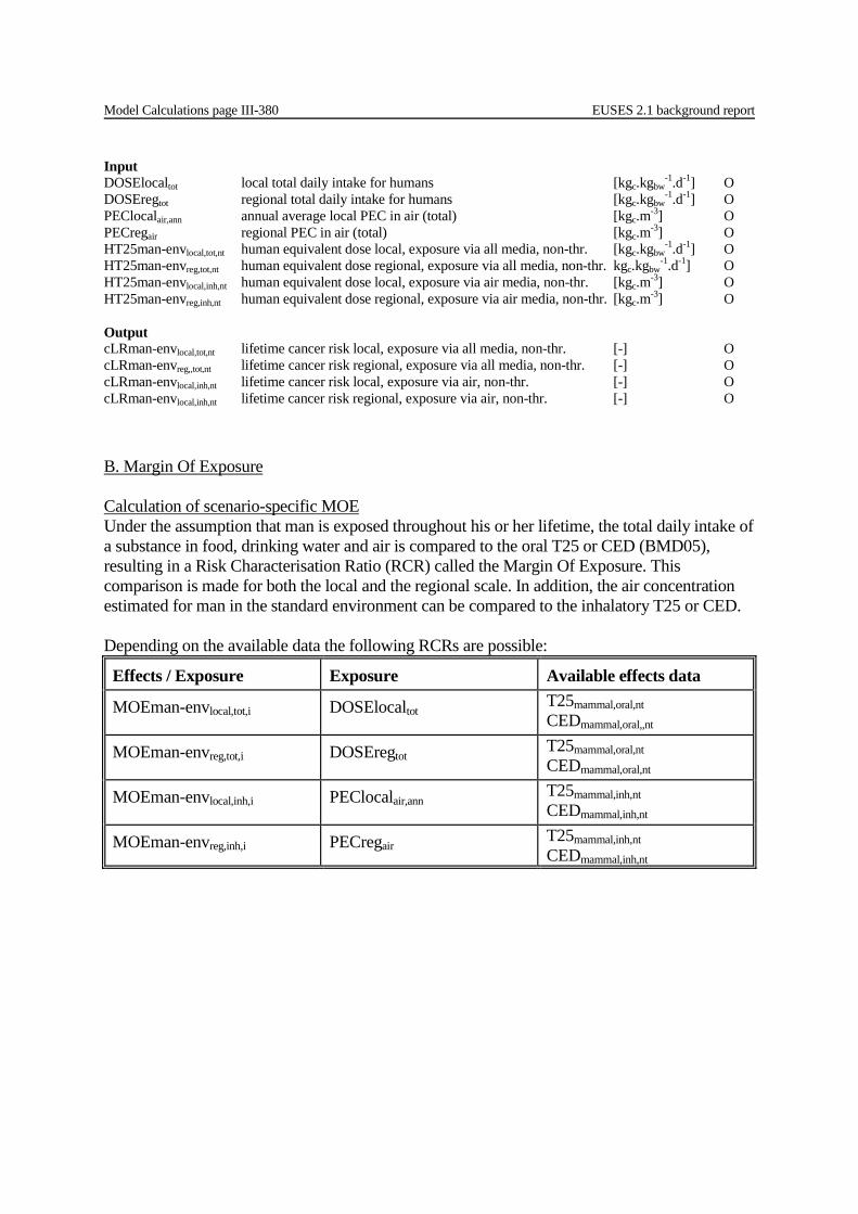
Model Calculations page III-380 EUSES 2.1 background report
Input DOSElocaltot local total daily intake for humans [kgc.kgbw
-1.d-1] O DOSEregtot regional total daily intake for humans [kgc.kgbw
-1.d-1] O PEClocalair,ann annual average local PEC in air (total) [kgc.m-3] O PECregair regional PEC in air (total) [kgc.m-3] O HT25man-envlocal,tot,nt human equivalent dose local, exposure via all media, non-thr. [kgc.kgbw
-1.d-1] O HT25man-envreg,tot,nt human equivalent dose regional, exposure via all media, non-thr. kgc.kgbw
-1.d-1] O HT25man-envlocal,inh,nt human equivalent dose local, exposure via air media, non-thr. [kgc.m-3] O HT25man-envreg,inh,nt human equivalent dose regional, exposure via air media, non-thr. [kgc.m-3] O Output cLRman-envlocal,tot,nt lifetime cancer risk local, exposure via all media, non-thr. [-] O cLRman-envreg,,tot,nt lifetime cancer risk regional, exposure via all media, non-thr. [-] O cLRman-envlocal,inh,nt lifetime cancer risk local, exposure via air, non-thr. [-] O cLRman-envlocal,inh,nt lifetime cancer risk regional, exposure via air, non-thr. [-] O B. Margin Of Exposure Calculation of scenario-specific MOE Under the assumption that man is exposed throughout his or her lifetime, the total daily intake of a substance in food, drinking water and air is compared to the oral T25 or CED (BMD05), resulting in a Risk Characterisation Ratio (RCR) called the Margin Of Exposure. This comparison is made for both the local and the regional scale. In addition, the air concentration estimated for man in the standard environment can be compared to the inhalatory T25 or CED. Depending on the available data the following RCRs are possible:
Effects / Exposure Exposure Available effects data
MOEman-envlocal,tot,i DOSElocaltot T25mammal,oral,nt CEDmammal,oral,,nt
MOEman-envreg,tot,i DOSEregtot T25mammal,oral,nt CEDmammal,oral,nt
MOEman-envlocal,inh,i PEClocalair,ann T25mammal,inh,nt CEDmammal,inh,nt
MOEman-envreg,inh,i PECregair T25mammal,inh,nt CEDmammal,inh,nt
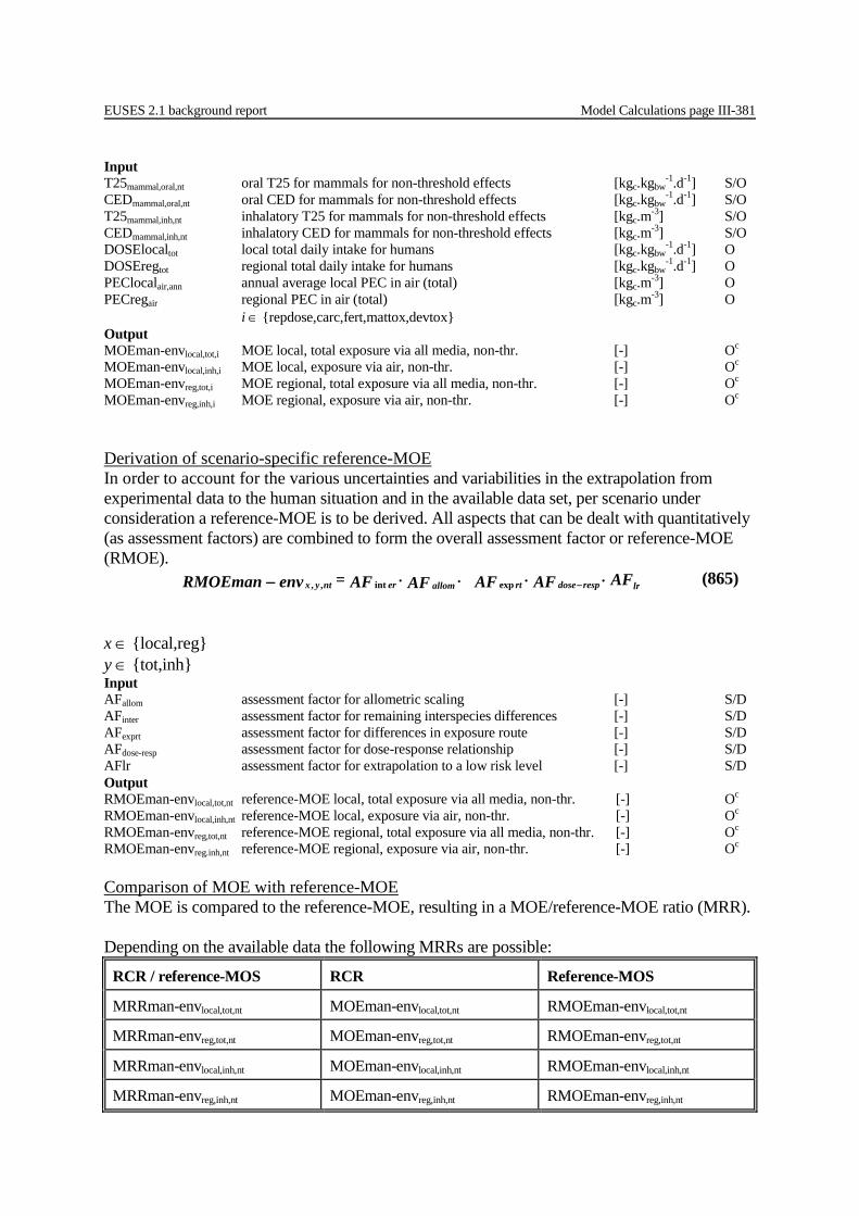
EUSES 2.1 background report Model Calculations page III-381
Input T25mammal,oral,nt oral T25 for mammals for non-threshold effects [kgc.kgbw
-1.d-1] S/O CEDmammal,oral,nt oral CED for mammals for non-threshold effects [kgc.kgbw
-1.d-1] S/O T25mammal,inh,nt inhalatory T25 for mammals for non-threshold effects [kgc.m-3] S/O CEDmammal,inh,nt inhalatory CED for mammals for non-threshold effects [kgc.m-3] S/O DOSElocaltot local total daily intake for humans [kgc.kgbw
-1.d-1] O DOSEregtot regional total daily intake for humans [kgc.kgbw
-1.d-1] O PEClocalair,ann annual average local PEC in air (total) [kgc.m-3] O PECregair regional PEC in air (total) [kgc.m-3] O i ∈ {repdose,carc,fert,mattox,devtox} Output MOEman-envlocal,tot,i MOE local, total exposure via all media, non-thr. [-] Oc MOEman-envlocal,inh,i MOE local, exposure via air, non-thr. [-] Oc MOEman-envreg,tot,i MOE regional, total exposure via all media, non-thr. [-] Oc MOEman-envreg,inh,i MOE regional, exposure via air, non-thr. [-] Oc Derivation of scenario-specific reference-MOE In order to account for the various uncertainties and variabilities in the extrapolation from experimental data to the human situation and in the available data set, per scenario under consideration a reference-MOE is to be derived. All aspects that can be dealt with quantitatively (as assessment factors) are combined to form the overall assessment factor or reference-MOE (RMOE). AF AF AF AF AF= envRMOEman lrrespdosertallomerntyx ⋅⋅⋅⋅− −expint,, (865)
x ∈ {local,reg} y ∈ {tot,inh} Input AFallom assessment factor for allometric scaling [-] S/D AFinter assessment factor for remaining interspecies differences [-] S/D AFexprt assessment factor for differences in exposure route [-] S/D AFdose-resp assessment factor for dose-response relationship [-] S/D AFlr assessment factor for extrapolation to a low risk level [-] S/D Output RMOEman-envlocal,tot,nt reference-MOE local, total exposure via all media, non-thr. [-] Oc RMOEman-envlocal,inh,nt reference-MOE local, exposure via air, non-thr. [-] Oc RMOEman-envreg,tot,nt reference-MOE regional, total exposure via all media, non-thr. [-] Oc RMOEman-envreg.inh,nt reference-MOE regional, exposure via air, non-thr. [-] Oc Comparison of MOE with reference-MOE The MOE is compared to the reference-MOE, resulting in a MOE/reference-MOE ratio (MRR). Depending on the available data the following MRRs are possible:
RCR / reference-MOS RCR Reference-MOS
MRRman-envlocal,tot,nt MOEman-envlocal,tot,nt RMOEman-envlocal,tot,nt
MRRman-envreg,tot,nt MOEman-envreg,tot,nt RMOEman-envreg,tot,nt
MRRman-envlocal,inh,nt MOEman-envlocal,inh,nt RMOEman-envlocal,inh,nt
MRRman-envreg,inh,nt MOEman-envreg,inh,nt RMOEman-envreg,inh,nt
Model Calculations page III-382 EUSES 2.1 background report
Input MOEman-envlocal,tot,,nt MOE local, total exposure via all media, non-thr. [-] Oc MOEman-envlocal,inh,nt MOE local, exposure via air, non-thr. [-] Oc MOEman-envreg,tot,nt MOE regional, total exposure via all media, non-thr. [-] Oc MOEman-envreg,inh,nt MOE regional, exposure via air, non-thr. [-] Oc RMOEman-envlocal,tot,nt reference-MOE local, total exposure via all media, non-thr. [-] Oc RMOEman-envlocal,inh,nt reference-MOE local, exposure via air, non-thr. [-] Oc RMOEman-envreg,tot,nt reference-MOE regional, total exposure via all media, non-thr. [-] Oc RMOEman-envreg.inh,nt reference-MOE regional, exposure via air, non-thr. [-] Oc Output MRRman-envlocal,tot,nt ratio MOE/RMOE local, total exposure via all media, non-thr. [-] Oc MRRman-envreg,tot,nt ratio MOE/RMOE regional, total exposure via all media, non-thr. [-] Oc MRRman-envlocal,inh,nt ratio MOE/RMOE local, exposure via air, non-thr. [-] Oc MRRman-envreg.inh,nt ratio MOE/RMOE regional, exposure via air, non-thr. [-] Oc
III.7.2.2 Risk characterisation for consumers III.7.2.2.1 Threshold substances MOS approach: Calculation of scenario-specific MOS The concentration of the substance in air, a medium swallowed or on the skin is compared to effect or no-effect concentrations of corresponding time scale and route of exposure. Likewise, a potential dermal uptake rate for a substance in contact with the skin and an intake rate for a substance in a medium swallowed are compared to effect or no-effect doses of corresponding time scale and route of exposure. See Section III.6.2.2 for decision rules on the choice of the effect parameter in the risk characterisation for human health. If both an N(L)OAEL for man and an N(L)OAEL for mammals are available, the former one is used in this risk characterisation. Note: Although in theory it is possible to calculate MOSs for the endpoints irritation/corrosivity and sensitisation, in practice the available toxicological database does not allow the derivation of a threshold for these endpoints. Therefore, MOS calculations for these endpoints have not been implemented in EUSES, but EUSES allows the user to flag substances for these properties (see Section III.6.2.2).
EUSES 2.1 background report Model Calculations page III-383
Inhalation exposure Depending on the time scale of the exposure scenario and available effects data the following RCRs are possible:
Effects / Exposure Exposure Available effects data
MOSconsinh,acute Cinh LC50mammal,inh NOAELman,inh,acute LOAELman,inh,acute
MOSconsinh,i Cinh,ann NOAELmammal,inh,i LOAELmammal,inh,i NOAELman,inh,i LOAELman,inh,i CEDmammal,inh,i
i ∈ {repdose,carc,fert,mattox,devtox} Input LC50mammal,inh inhalatory LC50 for mammals [kgc.m-3] S N(L)OAELman,inh,acute inhalatory N(L)OAEL for man for acute effects [kgc.m-3] S N(L)OAELmammal,inh,i inhalatory N(L)OAEL for mammals for endpoint of concern [kgc.m-3] S/O N(L)OAELman,inh,i inhalatory N(L)OAEL for man for endpoint of concern [kgc.m-3] S/O CEDmammal,inh,i inhalatory CED for mammals for endpoint of concern [kgc.m-3] S Cinh concentration in air of room [kgc.m-3] O Cinh,ann annual average inhalation exposure concentration [kgc.m-3] O i ∈ {repdose,carc,fert,mattox,devtox} Output MOSconsinh,acute MOS acute, inhalatory exposure [-] Oc MOSconsinh,i MOS for endpoint of concern, inhalatory exposure [-] Oc i ∈ {repdose,carc,fert,mattox,devtox}
Model Calculations page III-384 EUSES 2.1 background report
Dermal exposure Depending on the time scale of the exposure scenario and available effects data the following RCRs are possible:
Effects / Exposure Exposure Available effects data
MOSconsder,acute Uder,pot LD50mammal,der NOAELman,der,acute LOAELman,der,acute
Cder NOECman,medium,acute LOECman,medium,acute
MOSconsder,i Uder,pot NOAELmammal,der,i LOAELmammal,der,i NOAELman,der,i LOAELman,der,i CEDmammal,der,i
Cder,ann NOECman,medium,i LOECman,medium,i
i ∈ {repdose,carc,fert,mattox,devtox} Input LD50mammal,der dermal LD50 for mammals [kgc.kgbw
-1] S N(L)OAELman,der,acute dermal N(L)OAEL for man for acute effects [kgc.kgbw
-1] S N(L)OECman,medium,acute dermal N(L)OEC in a medium for man for acute effects [kgc.m-3] S N(L)OAELmammal,der,i dermal N(L)OAEL for mammals for endpoint of concern [kgc.kgbw
-1.d-1] S/O N(L)OAELman,der,i dermal N(L)OAEL for man for endpoint of concern [kgc.kgbw
-1.d-1] S/O CEDmammal,der,i dermal CED for mammals for endpoint of concern [kgc.kgbw
-1.d-1] S N(L)OECman,medium,i dermal N(L)OEC in a medium for man for endpoint of concern [kgc.m-3] S Uder,pot potential dermal uptake rate [kgc.kgbw
-1.d-1] O Cder concentration of substance in product on skin [kgc.m-3] O Cder,ann annual average dermal exposure concentration [kgc.m-3] O i ∈ {repdose,carc,fert,mattox,devtox} Output MOSconsder,acute MOS acute, dermal exposure [-] Oc MOSconsder,i MOS for endpoint of concern, dermal exposure [-] Oc i ∈ {repdose,carc,fert,mattox,devtox}
EUSES 2.1 background report Model Calculations page III-385
Oral exposure Depending on the time scale of the exposure scenario and available effects data the following RCRs are possible:
Effects / Exposure Exposure Available effects data
MOSconsoral,acute Ioral LD50mammal,oral DDmammal,oral NOAELman,oral,acute LOAELman,oral,acute
MOSconsoral,i Ioral NOAELmammal,oral,i LOAELmammal,oral,i NOAELman,oral,i LOAELman,oral,i CEDmammal,oral,i
Coral,ann / RHOprod NOECmammal,food,i LOECmammal,food,i
i ∈ {repdose,carc,fert,mattox,devtox} Input LD50mammal,oral oral LD50 for mammals [kgc.kgbw
-1] S DDmammal,oral oral Discriminating Dose for mammals [kgc.kgbw
-1] S N(L)OAELman,oral,acute oral N(L)OAEL for man for acute effects [kgc.kgbw
-1] S N(L)OAELmammal,oral,i oral N(L)OAEL for mammals for endpoint of concern [kgc.kgbw
-1.d-1] S/O N(L)OAELman,oral,i oral N(L)OAEL for man for endpoint of concern [kgc.kgbw
-1.d-1] S/O CEDmammal,oral,i oral CED for mammals for endpoint of concern [kgc.kgbw
-1.d-1] S N(L)OECmammal,food,i N(L)OEC via food for mammals for endpoint of concern [kgc.kgfood
-1] S RHOprod density of product before dilution [kg.m-3] S Ioral ingestion rate of substance [kgc.kgbw
-1.d-1] O Coral,ann annual average oral exposure concentration [kgc.m-3] O i ∈ {repdose,carc,fert,mattox,devtox} Output MOSconsoral,acute MOS acute, oral exposure [-] Oc MOSconsoral,i MOS for endpoint of concern, oral exposure [-] Oc i ∈ {repdose,carc,fert,mattox,devtox}
Model Calculations page III-386 EUSES 2.1 background report
Total exposure via all routes Depending on the time scale and available effects data the following RCRs are possible:
Effects / Exposure Exposure Available effects data
MOSconstot,acute Utot / BIOoral,2 LD50mammal,oral DDmammal,oral NOAELman,oral,acute LOAELman,oral,acute
MOSconstot,i Utot / BIOoral,2 NOAELmammal,oral,i LOAELmammal,oral,i NOAELman,oral,i LOAELman,oral,i CEDmammal,oral,i
i ∈ {repdose,carc,fert,mattox,devtox} Input LD50mammal,oral oral LD50 for mammals [kgc.kgbw
-1] S DDmammal,oral oral Discriminating Dose for mammals [kgc.kgbw
-1] S N(L)OAELman,oral,acute oral N(L)OAEL for man for acute effects [kgc.kgbw
-1] S N(L)OAELmammal,oral,i oral N(L)OAEL for mammals for endpoint of concern [kgc.kgbw
-1.d-1] S/O N(L)OAELman,oral,i oral N(L)OAEL for man for endpoint of concern [kgc.kgbw
-1.d-1] S/O CEDmammal,oral,i oral CED for mammals for endpoint of concern [kgc.kgbw
-1.d-1] S BIOoral,2 bioavailability for oral uptake (starting route) [-] S/D Utot total uptake for one product via different routes [kgc.kgbw
-1.d-1] O i ∈ {repdose,carc,fert,mattox,devtox} Output MOSconstot,acute MOS acute, total exposure [-] Oc MOSconstot,i MOS for endpoint of concern, total exposure [-] Oc i ∈ {repdose,carc,fert,mattox,devtox} Derivation of scenario-specific reference-MOS In order to account for the various uncertainties and variabilities in the extrapolation from experimental data to the human situation and in the available data set, per scenario under consideration a reference-MOS is to be derived. All aspects that can be dealt with quantitatively (as assessment factors) are combined to form the overall assessment factor or reference-MOS (RMOS).
y ∈ {inh,der,oral,tot} i ∈ {repdose,carc,fert,mattox,devtox}
AF AF AF AF AF AF= RMOScons respdosertdurallom raeracutey −⋅⋅⋅⋅⋅ expexpintint, (866)
AF AF AF AF AF AF= RMOScons respdosertdurallom raeriy −⋅⋅⋅⋅⋅ expexpintint, (867)
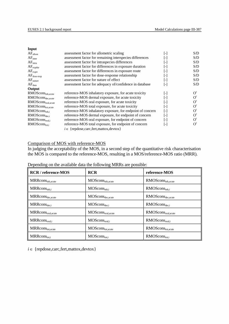
EUSES 2.1 background report Model Calculations page III-387
Input AFallom assessment factor for allometric scaling [-] S/D AFinter assessment factor for remaining interspecies differences [-] S/D AFintra assessment factor for intraspecies differences [-] S/D AFexpdur assessment factor for differences in exposure duration [-] S/D AFexprt assessment factor for differences in exposure route [-] S/D AFdose-resp assessment factor for dose-response relationship [-] S/D AFnature assessment factor for nature of effect [-] S/D AFdata assessment factor for adequacy of/confidence in database [-] S/D Output RMOSconsinh,acute reference-MOS inhalatory exposure, for acute toxicity [-] Oc
RMOSconsder,acute reference-MOS dermal exposure, for acute toxicity [-] Oc RMOSconsoral,acute reference-MOS oral exposure, for acute toxicity [-] Oc RMOSconstot,acute reference-MOS total exposure, for acute toxicity [-] Oc RMOSconsinh,i reference-MOS inhalatory exposure, for endpoint of concern [-] Oc RMOSconsder,i reference-MOS dermal exposure, for endpoint of concern [-] Oc RMOSconsoral,i reference-MOS oral exposure, for endpoint of concern [-] Oc RMOSconstot,i reference-MOS total exposure, for endpoint of concern [-] Oc i ∈ {repdose,carc,fert,mattox,devtox} Comparison of MOS with reference-MOS In judging the acceptability of the MOS, in a second step of the quantitative risk characterisation the MOS is compared to the reference-MOS, resulting in a MOS/reference-MOS ratio (MRR). Depending on the available data the following MRRs are possible:
RCR / reference-MOS RCR reference-MOS
MRRconsinh,acute MOSconsinh,acute RMOSconsinh,acute
MRRconsinh,i MOSconsinh,i RMOSconsinh,i
MRRconsder,acute MOSconsder,acute RMOSconsder,acute
MRRconsder,i MOSconsder,i RMOSconsder,i
MRRconsoral,acute MOSconsoral,acute RMOSconsoral,acute
MRRconsoral,i MOSconsoral,i RMOSconsoral,i
MRRconstot,acute MOSconstot,acute RMOSconstot,acute
MRRconstot,i MOSconstot,i RMOSconstot,i
i ∈ {repdose,carc,fert,mattox,devtox}
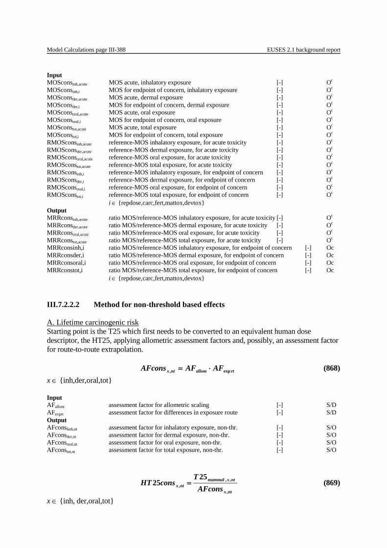
Model Calculations page III-388 EUSES 2.1 background report
Input MOSconsinh,acute MOS acute, inhalatory exposure [-] Oc MOSconsinh,i MOS for endpoint of concern, inhalatory exposure [-] Oc MOSconsder,acute MOS acute, dermal exposure [-] Oc MOSconsder,i MOS for endpoint of concern, dermal exposure [-] Oc MOSconsoral,acute MOS acute, oral exposure [-] Oc MOSconsoral,i MOS for endpoint of concern, oral exposure [-] Oc MOSconstot,acute MOS acute, total exposure [-] Oc MOSconstot,i MOS for endpoint of concern, total exposure [-] Oc RMOSconsinh,acute reference-MOS inhalatory exposure, for acute toxicity [-] Oc RMOSconsder,acute reference-MOS dermal exposure, for acute toxicity [-] Oc RMOSconsoral,acute reference-MOS oral exposure, for acute toxicity [-] Oc RMOSconstot,acute reference-MOS total exposure, for acute toxicity [-] Oc RMOSconsinh,i reference-MOS inhalatory exposure, for endpoint of concern [-] Oc RMOSconsder,i reference-MOS dermal exposure, for endpoint of concern [-] Oc RMOSconsoral,i reference-MOS oral exposure, for endpoint of concern [-] Oc RMOSconstot,i reference-MOS total exposure, for endpoint of concern [-] Oc i ∈ {repdose,carc,fert,mattox,devtox} Output MRRconsinh,acute ratio MOS/reference-MOS inhalatory exposure, for acute toxicity [-] Oc MRRconsder,acute ratio MOS/reference-MOS dermal exposure, for acute toxicity [-] Oc MRRconsoral,acute ratio MOS/reference-MOS oral exposure, for acute toxicity [-] Oc MRRconstot,acute ratio MOS/reference-MOS total exposure, for acute toxicity [-] Oc MRRconsinh,i ratio MOS/reference-MOS inhalatory exposure, for endpoint of concern [-] Oc MRRconsder,i ratio MOS/reference-MOS dermal exposure, for endpoint of concern [-] Oc MRRconsoral,i ratio MOS/reference-MOS oral exposure, for endpoint of concern [-] Oc MRRconstot,i ratio MOS/reference-MOS total exposure, for endpoint of concern [-] Oc i ∈ {repdose,carc,fert,mattox,devtox} III.7.2.2.2 Method for non-threshold based effects A. Lifetime carcinogenic risk Starting point is the T25 which first needs to be converted to an equivalent human dose descriptor, the HT25, applying allometric assessment factors and, possibly, an assessment factor for route-to-route extrapolation. rtallomntx AFAFAFcons exp, ⋅= (868) x ∈ {inh,der,oral,tot} Input AFallom assessment factor for allometric scaling [-] S/D AFexprt assessment factor for differences in exposure route [-] S/D Output AFconslinh,nt assessment factor for inhalatory exposure, non-thr. [-] S/O AFconsder,nt assessment factor for dermal exposure, non-thr. [-] S/O AFconsoral,nt assessment factor for oral exposure, non-thr. [-] S/O AFconstot,nt assessment factor for total exposure, non-thr. [-] S/O
ntx
ntxmammalntx AFcons
TconsHT
,
,,,
2525 = (869)
x ∈ {inh, der,oral,tot}
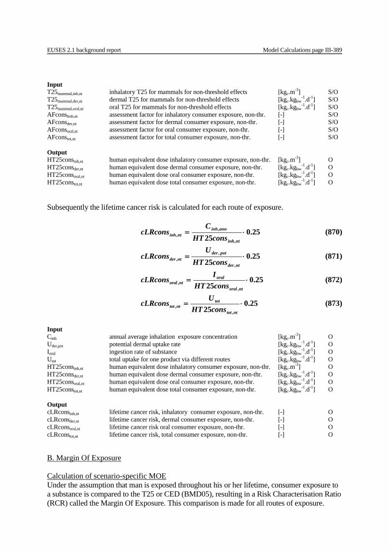
EUSES 2.1 background report Model Calculations page III-389
Input T25mammal,inh,nt inhalatory T25 for mammals for non-threshold effects [kgc.m-3] S/O T25mammal,der,nt dermal T25 for mammals for non-threshold effects [kgc.kgbw
-1.d-1] S/O T25mammal,oral,nt oral T25 for mammals for non-threshold effects [kgc.kgbw
-1.d-1] S/O AFconslinh,nt assessment factor for inhalatory consumer exposure, non-thr. [-] S/O AFconsder,nt assessment factor for dermal consumer exposure, non-thr. [-] S/O AFconsoral,nt assessment factor for oral consumer exposure, non-thr. [-] S/O AFconstot,nt assessment factor for total consumer exposure, non-thr. [-] S/O Output HT25consinh,nt human equivalent dose inhalatory consumer exposure, non-thr. [kgc.m-3] O HT25consder,nt human equivalent dose dermal consumer exposure, non-thr. [kgc.kgbw
-1.d-1] O HT25consoral,nt human equivalent dose oral consumer exposure, non-thr. [kgc.kgbw
-1.d-1] O HT25constot,nt human equivalent dose total consumer exposure, non-thr. [kgc.kgbw
-1.d-1] O
Subsequently the lifetime cancer risk is calculated for each route of exposure.
25.025 ,
,, ⋅=
ntinh
anninhntinh consHT
CcLRcons (870)
25.025 ,
,, ⋅=
ntder
potderntder consHT
UcLRcons (871)
25.025 ,
, ⋅=ntoral
oralntoral consHT
IcLRcons (872)
25.025 ,
, ⋅=nttot
totnttot consHT
UcLRcons (873)
Input Cinh annual average inhalation exposure concentration [kgc.m-3] O Uder,pot potential dermal uptake rate [kgc.kgbw
-1.d-1] O Ioral ingestion rate of substance [kgc.kgbw
-1.d-1] O Utot total uptake for one product via different routes [kgc.kgbw
-1.d-1] O HT25consinh,nt human equivalent dose inhalatory consumer exposure, non-thr. [kgc.m-3] O HT25consder,nt human equivalent dose dermal consumer exposure, non-thr. [kgc.kgbw
-1.d-1] O HT25consoral,nt human equivalent dose oral consumer exposure, non-thr. [kgc.kgbw
-1.d-1] O HT25constot,nt human equivalent dose total consumer exposure, non-thr. [kgc.kgbw
-1.d-1] O Output cLRconsinh,nt lifetime cancer risk, inhalatory consumer exposure, non-thr. [-] O cLRconsder,nt lifetime cancer risk, dermal consumer exposure, non-thr. [-] O cLRconsoral,nt lifetime cancer risk oral consumer exposure, non-thr. [-] O cLRconstot,nt lifetime cancer risk, total consumer exposure, non-thr. [-] O B. Margin Of Exposure Calculation of scenario-specific MOE Under the assumption that man is exposed throughout his or her lifetime, consumer exposure to a substance is compared to the T25 or CED (BMD05), resulting in a Risk Characterisation Ratio (RCR) called the Margin Of Exposure. This comparison is made for all routes of exposure.

Model Calculations page III-390 EUSES 2.1 background report
Depending on the available data the following RCRs are possible:
Effects / Exposure Exposure Available effects data
MOEconsinh,nt Cinh,ann T25mammal,inh,nt CEDmammal,inh,,nt
MOEconsder,nt Uder,pot T25mammal,der,nt CEDmammal,der,nt
MOEconsoral,nt Ioral T25mammal,oral,nt CEDmammal,oral,nt
MOEconstot,nt Utot/BIOoral,2 T25mammal,oral,nt CEDmammal,oral,nt
Input T25mammal,inh,nt inhalatory T25 for mammals for non-threshold effects [kgc.m-3] S/O CEDmammal,inh,nt inhalatory CED for mammals for non-threshold effects [kgc.m-3] S/O T25mammal,der,nt dermal T25 for mammals for non-threshold effects [kgc.kgbw
-1.d-1] S/O CEDmammal,der,nt dermal CED for mammals for non-threshold effects [kgc.kgbw
-1.d-1] S/O T25mammal,oral,nt oral T25 for mammals for non-threshold effects [kgc.kgbw
-1.d-1] S/O CEDmammal,oral,nt oral CED for mammals for non-threshold effects [kgc.kgbw
-1.d-1] S/O Cinh annual average inhalation exposure concentration [kgc.m-3] O Uder,pot potential dermal uptake rate [kgc.kgbw
-1.d-1] O Ioral ingestion rate of substance [kgc.kgbw
-1.d-1] O Utot total uptake for one product via different routes [kgc.kgbw
-1.d-1] O BIOoral,2 bioavailability for oral uptake, starting route Output MOEconsinh,nt MOE inhalatory consumer exposure, non-thr. [-] Oc MOEconsder,nt MOE dermal consumer exposure, non-thr. [-] Oc MOEconsoral,nt MOE oral consumer exposure, non-thr. [-] Oc MOEconstot,nt MOE total consumer exposure, non-thr. [-] Oc Derivation of scenario-specific reference-MOE In order to account for the various uncertainties and variabilities in the extrapolation from experimental data to the consumer situation and in the available data set, per scenario under consideration a reference-MOE is to be derived. All aspects that can be dealt with quantitatively (as assessment factors) are combined to form the overall assessment factor or reference-MOE (RMOE). AF AF AFAF AF= RMOEcons lrrespdosertallomerntx ⋅⋅⋅⋅ −expint, (874)
x ∈ {inh,der,oral,tot}

EUSES 2.1 background report Model Calculations page III-391
Input AFallom assessment factor for allometric scaling [-] S/D AFinter assessment factor for remaining interspecies differences [-] S/D AFexprt assessment factor for differences in exposure route [-] S/D AFdose-resp assessment factor for dose-response relationship [-] S/D AFlr assessment factor for extrapolation to a low risk level [-] S/D Output RMOEconsinh,nt reference-MOE inhalatory consumer exposure, non-thr. [-] Oc RMOEconsder,nt reference-MOE dermal consumer exposure, non-thr. [-] Oc RMOEconsoral,nt reference-MOE oral consumer exposure, non-thr. [-] Oc RMOEconstot,nt reference-MOE total consumer exposure, non-thr. [-] Oc Comparison of MOE with reference-MOE The MOE is compared to the reference-MOE, resulting in a MOE/reference-MOE ratio (MRR). Depending on the available data the following MRRs are possible:
RCR / reference-MOS RCR Reference-MOS
MRRconsinh,nt MOEconsinh,nt RMOEconsinh,nt
MRRconsder,nt MOEconsder,nt RMOEconsder,nt
MRRconsoral,nt MOEconsoral,nt RMOEconsoral,nt
MRRconstot,nt MOEconstot,nt RMOEconstot,nt
Input MOEconsinh,nt MOE inhalatory consumer exposure, non-thr. [-] Oc MOEconsder,nt MOE dermal consumer exposure, non-thr. [-] Oc MOEconsoral,nt MOE oral consumer exposure, non-thr. [-] Oc MOEconstot,nt MOE total consumer exposure, non-thr. [-] Oc RMOEconsinh,nt reference-MOE inhalatory consumer exposure, non-thr. [-] Oc RMOEconsder,nt reference-MOE dermal consumer exposure, non-thr. [-] Oc RMOEconsoral,nt reference-MOE oral consumer exposure, non-thr. [-] Oc RMOEconstot,nt reference-MOE total consumer exposure, non-thr. [-] Oc Output MRRconsinh,nt ratio MOE/RMOE, inhalatory consumer exposure, non-thr. [-] Oc MRRconsder,nt ratio MOE/RMOE, dermal consumer exposure, non-thr. [-] Oc MRRconsoral,nt ratio MOE/RMOE, oral consumer exposure, non-thr. [-] Oc MRRconstot,nt ratio MOE/RMOE, total consumer exposure, non-thr. [-] Oc
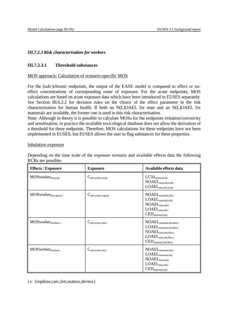
Model Calculations page III-392 EUSES 2.1 background report
III.7.2.3 Risk characterisation for workers III.7.2.3.1 Threshold substances MOS approach: Calculation of scenario-specific MOS For the (sub-)chronic endpoints, the output of the EASE model is compared to effect or no-effect concentrations of corresponding route of exposure. For the acute endpoints, MOS calculations are based on acute exposure data which have been introduced in EUSES separately. See Section III.6.2.2 for decision rules on the choice of the effect parameter in the risk characterisation for human health. If both an N(L)OAEL for man and an N(L)OAEL for mammals are available, the former one is used in this risk characterisation. Note: Although in theory it is possible to calculate MOSs for the endpoints irritation/corrosivity and sensitisation, in practice the available toxicological database does not allow the derivation of a threshold for these endpoints. Therefore, MOS calculations for these endpoints have not been implemented in EUSES, but EUSES allows the user to flag substances for these properties. Inhalation exposure Depending on the time scale of the exposure scenario and available effects data the following RCRs are possible:
Effects / Exposure Exposure Available effects data
MOSworkerinh,acute Cinh,worker,acute
LC50mammal,inh NOAELman,inh,acute LOAELman,inh,acute
MOSworkerinh,vapour,i Cinh,worker,vapour NOAELmammal,inh,i LOAELmammal,inh,i NOAELman,inh,i LOAELman,inh,i CEDmammal,inh,i
MOSworkerinh,fibre,i Cinh,worker,fibre NOAELmammal,inh,fibre,i LOAELmammal,inh,fibre,i NOAELman,inh,fibre,i LOAELman,inh,fibre,i CEDmammal,inh,fibre,i
MOSworkerinh,dust,i Cinh,worker,dust NOAELmammal,inh,i LOAELmammal,inh,i NOAELman,inh,i LOAELman,inh,i CEDmammal,inh,i
i ∈ {repdose,carc,fert,mattox,devtox}

EUSES 2.1 background report Model Calculations page III-393
Input LC50mammal,inh inhalatory LC50 for mammals [kgc.m-3] S N(L)OAELman,inh,acute inhalatory N(L)OAEL for man for acute effects [kgc.m-3] S N(L)OAELmammal,inh,i inhalatory N(L)OAEL for mammals for endpoint of concern [kgc.m-3] S/O N(L)OAELman,inh,i inhalatory N(L)OAEL for man for endpoint of concern [kgc.m-3] S/O CEDmammal,inh,i inhalatory CED for mammals for endpoint of concern [kgc.m-3] S N(L)OAELmammal,inh,fibre,i inh. N(L)OAEL for mammals exposed to fibers for endpoint of concern [fibers.m-3] S N(L)OAELman,inh,fibre,i inh. N(L)OAEL for man exposed to fibers for endpoint of concern [fibers.m-3] S CEDmammal,inh,fibre,i inh. CED for mammals exposed to fibers for endpoint of concern [fibers.m-3] S Cinh,worker,acute concentration in air for workers, acute exposure [kg.m-3] S Cinh,worker,vapour vapour concentration in air for workers [kg.m-3] O Cinh,worker,fibre fibre concentration in air for workers [fibers.m-3] O Cinh,worker,dust dust concentration in air for workers [kg.m-3] O i ∈ {repdose,carc,fert,mattox,devtox} Output MOSworkerinh,acute MOS acute, inhalatory exposure [-] Oc MOSworkerinh,vapour,i MOS for endpoint of concern, inhalatory exposure of vapour [-] Oc MOSworkerinh,fibre,i MOS for endpoint of concern, inhalatory exposure of fibers [-] Oc MOSworkerinh,dust,i MOS for endpoint of concern, inhalatory exposure of dust [-] Oc i ∈ {repdose,carc,fert,mattox,devtox} Dermal exposure Depending on the time scale of the exposure scenario and available effects data the following RCRs are possible:
Effects / Exposure Exposure Available effects data
MOSworkerder,acute Uder,pot,worker,acute LD50mammal,der NOAELman,der,acute LOAELman,der,acute
Wder,worker,acute / (THder,worker ⋅ nworker)
NOECman,medium,acute LOECman,medium,acute
MOSworkerder,i Uder,pot,worker NOAELmammal,der,i LOAELmammal,der,i NOAELman,der,i LOAELman,der,i CEDmammal,der,i
Wder,worker / (THder,worker ⋅ nworker) NOECman,medium,i LOECman,medium,i
i ∈ {repdose,carc,fert,mattox,devtox}
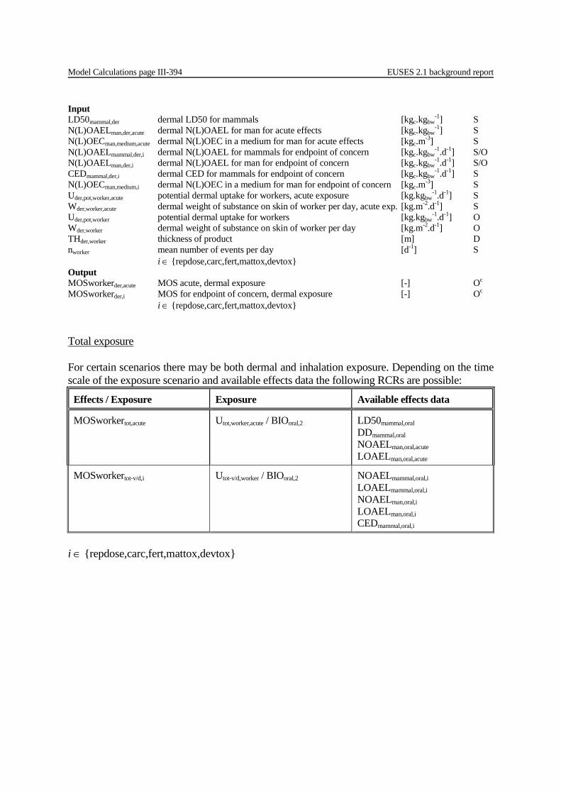
Model Calculations page III-394 EUSES 2.1 background report
Input LD50mammal,der dermal LD50 for mammals [kgc.kgbw
-1] S N(L)OAELman,der,acute dermal N(L)OAEL for man for acute effects [kgc.kgbw
-1] S N(L)OECman,medium,acute dermal N(L)OEC in a medium for man for acute effects [kgc.m-3] S N(L)OAELmammal,der,i dermal N(L)OAEL for mammals for endpoint of concern [kgc.kgbw
-1.d-1] S/O N(L)OAELman,der,i dermal N(L)OAEL for man for endpoint of concern [kgc.kgbw
-1.d-1] S/O CEDmammal,der,i dermal CED for mammals for endpoint of concern [kgc.kgbw
-1.d-1] S N(L)OECman,medium,i dermal N(L)OEC in a medium for man for endpoint of concern [kgc.m-3] S Uder,pot,worker,acute potential dermal uptake for workers, acute exposure [kg.kgbw
-1.d-1] S Wder,worker,acute dermal weight of substance on skin of worker per day, acute exp. [kg.m-2.d-1] S Uder,pot,worker potential dermal uptake for workers [kg.kgbw
-1.d-1] O Wder,worker dermal weight of substance on skin of worker per day [kg.m-2.d-1] O THder,worker thickness of product [m] D nworker mean number of events per day [d-1] S i ∈ {repdose,carc,fert,mattox,devtox} Output MOSworkerder,acute MOS acute, dermal exposure [-] Oc MOSworkerder,i MOS for endpoint of concern, dermal exposure [-] Oc i ∈ {repdose,carc,fert,mattox,devtox} Total exposure For certain scenarios there may be both dermal and inhalation exposure. Depending on the time scale of the exposure scenario and available effects data the following RCRs are possible:
Effects / Exposure Exposure Available effects data
MOSworkertot,acute Utot,worker,acute / BIOoral,2 LD50mammal,oral DDmammal,oral NOAELman,oral,acute LOAELman,oral,acute
MOSworkertot-v/d,i Utot-v/d,worker / BIOoral,2 NOAELmammal,oral,i LOAELmammal,oral,i NOAELman,oral,i LOAELman,oral,i CEDmammal,oral,i
i ∈ {repdose,carc,fert,mattox,devtox}
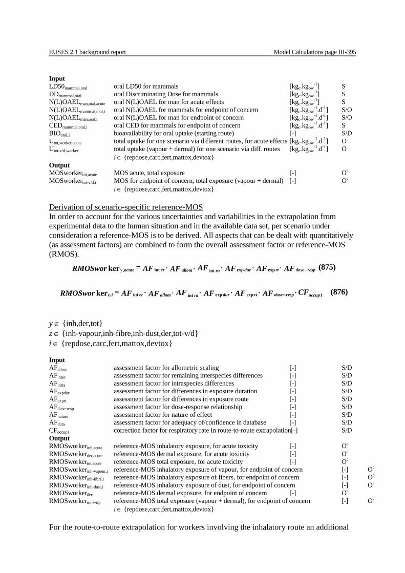
EUSES 2.1 background report Model Calculations page III-395
Input LD50mammal,oral oral LD50 for mammals [kgc.kgbw
-1] S DDmammal,oral oral Discriminating Dose for mammals [kgc.kgbw
-1] S N(L)OAELman,oral,acute oral N(L)OAEL for man for acute effects [kgc.kgbw
-1] S N(L)OAELmammal,oral,i oral N(L)OAEL for mammals for endpoint of concern [kgc.kgbw
-1.d-1] S/O N(L)OAELman,oral,i oral N(L)OAEL for man for endpoint of concern [kgc.kgbw
-1.d-1] S/O CEDmammal,oral,i oral CED for mammals for endpoint of concern [kgc.kgbw
-1.d-1] S BIOoral,2 bioavailability for oral uptake (starting route) [-] S/D Utot,worker,acute total uptake for one scenario via different routes, for acute effects [kgc.kgbw
-1.d-1] O Utot-v/d,worker total uptake (vapour + dermal) for one scenario via diff. routes [kgc.kgbw
-1.d-1] O i ∈ {repdose,carc,fert,mattox,devtox} Output MOSworkertot,acute MOS acute, total exposure [-] Oc MOSworkertot-v/d,i MOS for endpoint of concern, total exposure (vapour + dermal) [-] Oc i ∈ {repdose,carc,fert,mattox,devtox} Derivation of scenario-specific reference-MOS In order to account for the various uncertainties and variabilities in the extrapolation from experimental data to the human situation and in the available data set, per scenario under consideration a reference-MOS is to be derived. All aspects that can be dealt with quantitatively (as assessment factors) are combined to form the overall assessment factor or reference-MOS (RMOS).
y ∈ {inh,der,tot} z ∈ {inh-vapour,inh-fibre,inh-dust,der,tot-v/d} i ∈ {repdose,carc,fert,mattox,devtox} Input AFallom assessment factor for allometric scaling [-] S/D AFinter assessment factor for remaining interspecies differences [-] S/D AFintra assessment factor for intraspecies differences [-] S/D AFexpdur assessment factor for differences in exposure duration [-] S/D AFexprt assessment factor for differences in exposure route [-] S/D AFdose-resp assessment factor for dose-response relationship [-] S/D AFnature assessment factor for nature of effect [-] S/D AFdata assessment factor for adequacy of/confidence in database [-] S/D CFoccup1 correction factor for respiratory rate in route-to-route extrapolation[-] S/D Output RMOSworkerinh,acute reference-MOS inhalatory exposure, for acute toxicity [-] Oc
RMOSworkerder,acute reference-MOS dermal exposure, for acute toxicity [-] Oc RMOSworkertot,acute reference-MOS total exposure, for acute toxicity [-] Oc RMOSworkerinh-vapour,i reference-MOS inhalatory exposure of vapour, for endpoint of concern [-] Oc RMOSworkerinh-fibre,i reference-MOS inhalatory exposure of fibers, for endpoint of concern [-] Oc RMOSworkerinh-dust,i reference-MOS inhalatory exposure of dust, for endpoint of concern [-] Oc RMOSworkerder,i reference-MOS dermal exposure, for endpoint of concern [-] Oc RMOSworkertot-v/d,i reference-MOS total exposure (vapour + dermal), for endpoint of concern [-] Oc i ∈ {repdose,carc,fert,mattox,devtox} For the route-to-route extrapolation for workers involving the inhalatory route an additional
AF AF AF AF AF AF= RMOSwor respdosertdurallom raeracutey −⋅⋅⋅⋅⋅ expexpintint,ker (875)
CF AF AF AF AF AF AF= RMOSwor occuprespdosertdurallom raeriz 1expexpintint,ker ⋅⋅⋅⋅⋅⋅ − (876)
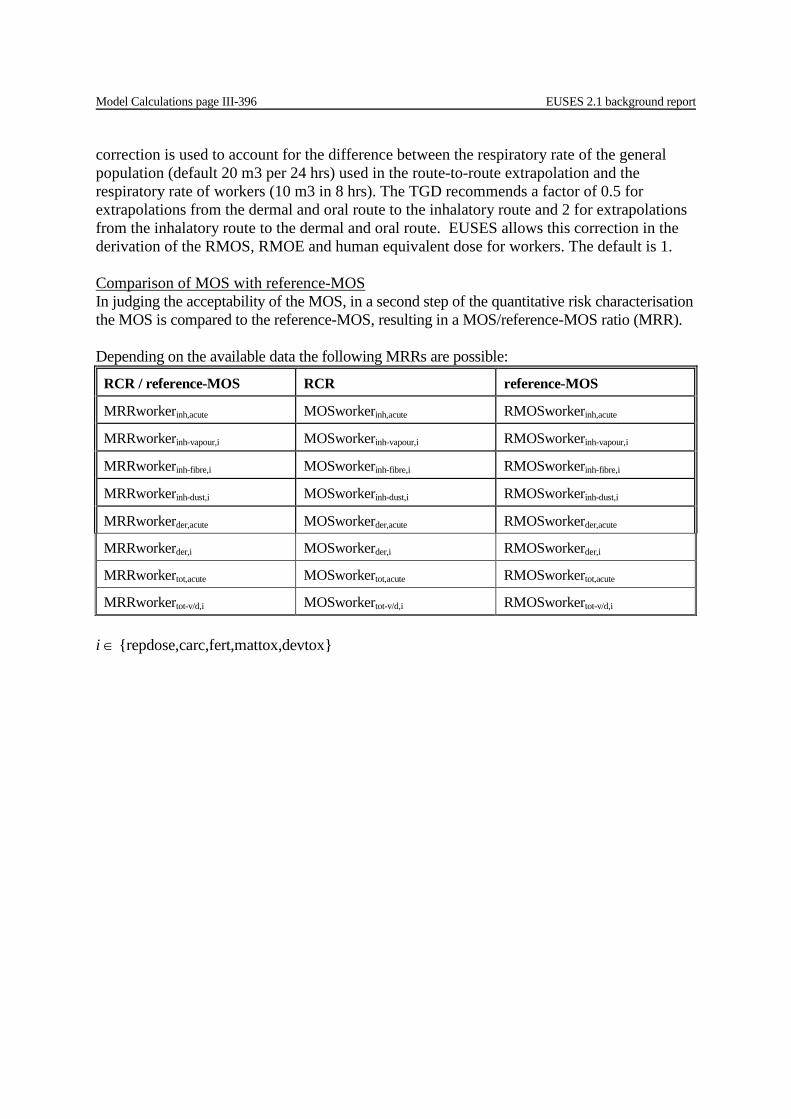
Model Calculations page III-396 EUSES 2.1 background report
correction is used to account for the difference between the respiratory rate of the general population (default 20 m3 per 24 hrs) used in the route-to-route extrapolation and the respiratory rate of workers (10 m3 in 8 hrs). The TGD recommends a factor of 0.5 for extrapolations from the dermal and oral route to the inhalatory route and 2 for extrapolations from the inhalatory route to the dermal and oral route. EUSES allows this correction in the derivation of the RMOS, RMOE and human equivalent dose for workers. The default is 1. Comparison of MOS with reference-MOS In judging the acceptability of the MOS, in a second step of the quantitative risk characterisation the MOS is compared to the reference-MOS, resulting in a MOS/reference-MOS ratio (MRR). Depending on the available data the following MRRs are possible:
RCR / reference-MOS RCR reference-MOS
MRRworkerinh,acute MOSworkerinh,acute RMOSworkerinh,acute
MRRworkerinh-vapour,i MOSworkerinh-vapour,i RMOSworkerinh-vapour,i
MRRworkerinh-fibre,i MOSworkerinh-fibre,i RMOSworkerinh-fibre,i
MRRworkerinh-dust,i MOSworkerinh-dust,i RMOSworkerinh-dust,i
MRRworkerder,acute MOSworkerder,acute RMOSworkerder,acute
MRRworkerder,i MOSworkerder,i RMOSworkerder,i
MRRworkertot,acute MOSworkertot,acute RMOSworkertot,acute
MRRworkertot-v/d,i MOSworkertot-v/d,i RMOSworkertot-v/d,i i ∈ {repdose,carc,fert,mattox,devtox}

EUSES 2.1 background report Model Calculations page III-397
Input MOSworkerinh,acute MOS acute, inhalatory exposure [-] Oc MOSworkerinh,vapour,i MOS for endpoint of concern, inhalatory exposure of vapour [-] Oc MOSworkerinh,fibre,i MOS for endpoint of concern, inhalatory exposure of fibers [-] Oc MOSworkerinh,dust,i MOS for endpoint of concern, inhalatory exposure of dust [-] Oc MOSworkerder,acute MOS acute, dermal exposure [-] Oc MOSworkerder,i MOS for endpoint of concern, dermal exposure [-] Oc MOSworkertot,acute MOS acute, total exposure [-] Oc MOSworkertot-v/d,i MOS for endpoint of concern, total exposure (vapour + dermal) [-] Oc RMOSworkerinh,acute reference-MOS inhalatory exposure, for acute toxicity [-] Oc RMOSworkerder,acute reference-MOS dermal exposure, for acute toxicity [-] Oc RMOSworkertot,acute reference-MOS total exposure, for acute toxicity [-] Oc RMOSworkerinh-vapour,i reference-MOS inhalatory exposure of vapour, for endpoint of concern [-] Oc RMOSworkerinh-fibre,i reference-MOS inhalatory exposure of fibers, for endpoint of concern [-] Oc RMOSworkerinh-dust,i reference-MOS inhalatory exposure of dust, for endpoint of concern [-] Oc RMOSworkerder,i reference-MOS dermal exposure, for endpoint of concern [-] Oc RMOSworkertot-v/d,i reference-MOS total exposure (vapour + dermal), for endpoint of concern [-] Oc i ∈ {repdose,carc,fert,mattox,devtox} Output MRRworkerinh,acute ratio MOS/reference-MOS inhalatory exposure, for acute toxicity [-] Oc MRRworkerder,acute ratio MOS/reference-MOS dermal exposure, for acute toxicity [-] Oc MRRworkertot,acute ratio MOS/reference-MOS total exposure, for acute toxicity [-] Oc MRRworkerinh-vapour,i ratio MOS/reference-MOS inhalatory exposure of vapour, for endpoint of concern [-] Oc MRRworkerinh-fibre,i ratio MOS/reference-MOS inhalatory exposure of fibers, for endpoint of concern [-] Oc MRRworkerinh-dust,i ratio MOS/reference-MOS inhalatory exposure of dust, for endpoint of concern [-] Oc MRRworkerder,i ratio MOS/reference-MOS dermal exposure, for endpoint of concern [-] Oc MRRworkertot-v/d,i ratio MOS/reference-MOS total exposure (vapour + dermal), for endpoint of concern [-] Oc i ∈ {repdose,carc,fert,mattox,devtox} III.7.2.3.2 Non-threshold substances A. Lifetime carcinogenic risk Starting point is the T25 which first needs to be converted to an equivalent human dose descriptor, the HT25, applying allometric assessment factors and, possibly, an assessment factor for route-to-route extrapolation. 1exp, .ker occuprtallomntx CFAFAFAFwor ⋅= (877)
x ∈ {inh-vapour,inh-fibre, inh-dust, der,tot-v/d} Input AFallom assessment factor for allometric scaling [-] S/D AFexprt assessment factor for differences in exposure route [-] S/D CFoccup1 correction factor for respiratory rate in route-to-route extrapolation[-] S/D Output AFworkerlinh-vaour,nt assessment factor for inhalatory worker vapour exposure, non-thr. [-] S/O AFworkerlinh-fibre,nt assessment factor for inhalatory worker fibre exposure, non-thr. [-] S/O AFworkerlinh-dust,nt assessment factor for inhalatory worker dust exposure, non-thr. [-] S/O AFworkerder,nt assessment factor for dermal worker exposure, non-thr. [-] S/O AFworkertot-v/d,nt assessment factor for total worker exposure, non-thr. [-] S/O
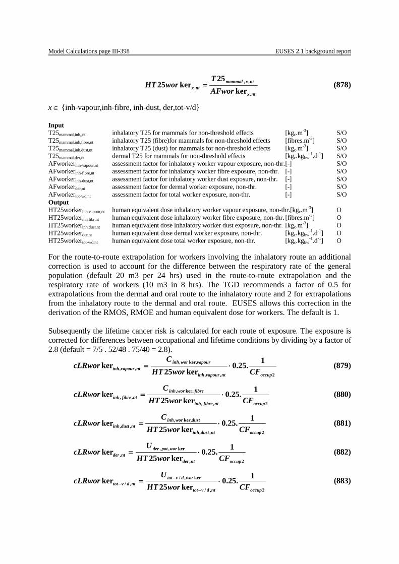
Model Calculations page III-398 EUSES 2.1 background report
ntx
ntxmammalntx AFwor
TworHT
,
,,, ker
25ker25 = (878)
x ∈ {inh-vapour,inh-fibre, inh-dust, der,tot-v/d} Input T25mammal,inh,,nt inhalatory T25 for mammals for non-threshold effects [kgc.m-3] S/O T25mammal,inh,fibre,nt inhalatory T25 (fibre)for mammals for non-threshold effects [fibres.m-3] S/O T25mammal,inh,dust,nt inhalatory T25 (dust) for mammals for non-threshold effects [kgc.m-3] S/O T25mammal,der,nt dermal T25 for mammals for non-threshold effects [kgc.kgbw
-1.d-1] S/O AFworkerinh-vapour,nt assessment factor for inhalatory worker vapour exposure, non-thr. [-] S/O AFworkerinh-fibre,nt assessment factor for inhalatory worker fibre exposure, non-thr. [-] S/O AFworkerinh-dust,nt assessment factor for inhalatory worker dust exposure, non-thr. [-] S/O AFworkerder,nt assessment factor for dermal worker exposure, non-thr. [-] S/O AFworkertot-v/d,nt assessment factor for total worker exposure, non-thr. [-] S/O Output HT25workerinh,vapour,nt human equivalent dose inhalatory worker vapour exposure, non-thr.[kgc.m-3] O HT25workerinh,fibr,nt human equivalent dose inhalatory worker fibre exposure, non-thr. [fibres.m-3] O HT25workerinh,dust,nt human equivalent dose inhalatory worker dust exposure, non-thr. [kgc.m-3] O HT25workerder,nt human equivalent dose dermal worker exposure, non-thr. [kgc.kgbw
-1.d-1] O HT25workertot-v/d,nt human equivalent dose total worker exposure, non-thr. [kgc.kgbw
-1.d-1] O
For the route-to-route extrapolation for workers involving the inhalatory route an additional correction is used to account for the difference between the respiratory rate of the general population (default 20 m3 per 24 hrs) used in the route-to-route extrapolation and the respiratory rate of workers (10 m3 in 8 hrs). The TGD recommends a factor of 0.5 for extrapolations from the dermal and oral route to the inhalatory route and 2 for extrapolations from the inhalatory route to the dermal and oral route. EUSES allows this correction in the derivation of the RMOS, RMOE and human equivalent dose for workers. The default is 1. Subsequently the lifetime cancer risk is calculated for each route of exposure. The exposure is corrected for differences between occupational and lifetime conditions by dividing by a factor of 2.8 (default = 7/5 . 52/48 . 75/40 = 2.8).
2,,
ker,,,,
1.25.0ker25
keroccupntvapourinh
vapourworinhntvapourinh CFworHT
CcLRwor ⋅= (879)
2,,
ker,,,,
1.25.0ker25
keroccupntfibreinh
fibreworinhntfibreinh CFworHT
CcLRwor ⋅= (880)
2,,
ker,,,,
1.25.0ker25
keroccupntdustinh
dustworinhntdustinh CFworHT
CcLRwor ⋅= (881)
2,
ker,,,
1.25.0ker25
keroccupntder
worpotderntder CFworHT
UcLRwor ⋅= (882)
2,/
ker,/,/
1.25.0ker25
keroccupntdvtot
wordvtotntdvtot CFworHT
UcLRwor ⋅=
−
−− (883)

EUSES 2.1 background report Model Calculations page III-399
Input Cinh,worker, vapour vapour concentration in air for workers [kgc.m-3] O Cinh,worker, fibre fibre concentration in air for workers [fibres.m-3] O Cinh,worker, dust dust concentration in air for workers [kgc.m-3] O Uder,pot,worker potential dermal uptake rate for workers [kgc.kgbw
-1.d-1] O Utot-v/d,worker total uptake for one scenario via different routes [kgc.kgbw
-1.d-1] O HT25workerinh,vapour,nt human equivalent dose inhalatory worker vapour exposure, non-thr.[kgc.m-3] O HT25workerinh,fibr,nt human equivalent dose inhalatory worker fibre exposure, non-thr. [fibres.m-3] O HT25workerinh,dust,nt human equivalent dose inhalatory worker dust exposure, non-thr. [kgc.m-3] O HT25workerder,nt human equivalent dose dermal worker exposure, non-thr. [kgc.kgbw
-1.d-1] O HT25workertot-v/d,nt human equivalent dose total worker exposure, non-thr. [kgc.kgbw
-1.d-1] O CFoccup2 correction factor for duration and frequency of exposure [-] D Output cLRconsinh,vaour,nt lifetime cancer risk, inhalatory worker vapour exposure, non-thr. [-] O cLRconsinh,fibre,nt lifetime cancer risk, inhalatory worker fibre exposure, non-thr. [-] O cLRconsinh,dust,nt lifetime cancer risk, inhalatory worker dust exposure, non-thr. [-] O cLRconsder,nt lifetime cancer risk, dermal worker exposure, non-thr. [-] O cLRconstot,nt lifetime cancer risk, total worker exposure, non-thr. [-] O B. Margin Of Exposure Calculation of scenario-specific MOE Under the assumption that man is exposed throughout his or her lifetime, exposure of workers to a substance is compared to the T25 or CED (BMD05), resulting in a Risk Characterisation Ratio (RCR) called the Margin Of Exposure. This comparison is made for all relevant routes of exposure. Depending on the available data the following RCRs are possible:
Effects / Exposure Exposure Available effects data
MOEworkerinh,vapour,nt Cinh,worker,vapour .1/CFoccup2 T25mammal,inh,nt CEDmammal,inh,nt
MOEworkerinh,fibre,nt Cinh,worker,fibre .1/CFoccup2 T25mammal,inh,fibre,nt CEDmammal,inh,fibre,nt
MOEworkerinh,dust,nt Cinh,worker,dust.1/CFoccup2 T25mammal,inh,dust,nt CEDmammal,inh,,dust,nt
MOEworkerder,nt Uder,pot,worker.1/CFoccup2 T25mammal,der,nt CEDmammal,der,nt
MOEworkertot-v/d,nt Utot-v/d,worker/(BIOoral,2 . CFoccup2) T25mammal,oral,nt CEDmammal,oral,nt
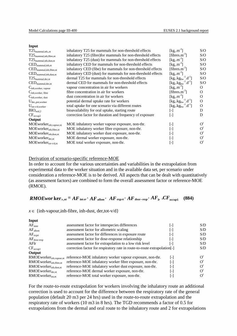
Model Calculations page III-400 EUSES 2.1 background report
Input T25mammal,inh,,nt inhalatory T25 for mammals for non-threshold effects [kgc.m-3] S/O T25mammal,inh,fibre,nt inhalatory T25 (fibre)for mammals for non-threshold effects [fibres.m-3] S/O T25mammal,inh,dust,nt inhalatory T25 (dust) for mammals for non-threshold effects [kgc.m-3] S/O CEDmammal,inh,nt inhalatory CED for mammals for non-threshold effects [kgc.m-3] S/O CEDmammal,inh,fibre,nt inhalatory CED (fibe) for mammals for non-threshold effects [fibres.m-3] S/O CEDmammal,inh,dust,nt inhalatory CED (dust) for mammals for non-threshold effects [kgc.m-3] S/O T25mammal,der,nt dermal T25 for mammals for non-threshold effects [kgc.kgbw
-1.d-1] S/O CEDmammal,der,nt dermal CED for mammals for non-threshold effects [kgc.kgbw
-1.d-1] S/O Cinh,worker, vapour vapour concentration in air for workers [kgc.m-3] O Cinh,worker, fibre fibre concentration in air for workers [fibres.m-3] O Cinh,worker, dust dust concentration in air for workers [kgc.m-3] O Uder,,pot,worker potential dermal uptake rate for workers [kgc.kgbw
-1.d-1] O Utot-v/d,worker total uptake for one scenario via different routes [kgc.kgbw
-1.d-1] O BIOoral,2 bioavailability for oral uptake, starting route [-] D CFoccup2 correction factor for duration and frequency of exposure [-] D Output MOEworkerinh,vapour,nt MOE inhalatory worker vapour exposure, non-thr. [-] Oc MOEworkerinh,fibre,nt MOE inhalatory worker fibre exposure, non-thr. [-] Oc MOEworkerinh,dust,nt MOE inhalatory worker dust exposure, non-thr. [-] Oc MOEworkerder,nt MOE dermal worker exposure, non-thr. [-] Oc MOEworkertot-v/d,nt MOE total worker exposure, non-thr. [-] Oc Derivation of scenario-specific reference-MOE In order to account for the various uncertainties and variabilities in the extrapolation from experimental data to the worker situation and in the available data set, per scenario under consideration a reference-MOE is to be derived. All aspects that can be dealt with quantitatively (as assessment factors) are combined to form the overall assessment factor or reference-MOE (RMOE).
CF AF AF AF AF AF= RMOEwor occuplrrespdosertallomerntx 1expint, .ker ⋅⋅⋅⋅ − (884)
x ∈ {inh-vapour,inh-fibre, inh-dust, der,tot-v/d} Input AFinter assessment factor for interspecies differences [-] S/D AFallom assessment factor for allometric scaling [-] S/D AFexprt assessment factor for differences in exposure route [-] S/D AFdose-resp assessment factor for dose-response relationship [-] S/D AFlr assessment factor for extrapolation to a low risk level [-] S/D CFoccup1 correction factor for respiratory rate in route-to-route extrapolation[-] S/D Output RMOEworkerinh,vapour,nt reference-MOE inhalatory worker vapour exposure, non-thr. [-] Oc RMOEworkerinh,fibre,nt reference-MOE inhalatory worker fibre exposure, non-thr. [-] Oc RMOEworkerinh,dust,nt reference-MOE inhalatory worker dust exposure, non-thr. [-] Oc RMOEworkerder,nt reference-MOE dermal worker exposure, non-thr. [-] Oc RMOEworkertot,nt reference-MOE total worker exposure, non-thr. [-] Oc For the route-to-route extrapolation for workers involving the inhalatory route an additional correction is used to account for the difference between the respiratory rate of the general population (default 20 m3 per 24 hrs) used in the route-to-route extrapolation and the respiratory rate of workers (10 m3 in 8 hrs). The TGD recommends a factor of 0.5 for extrapolations from the dermal and oral route to the inhalatory route and 2 for extrapolations
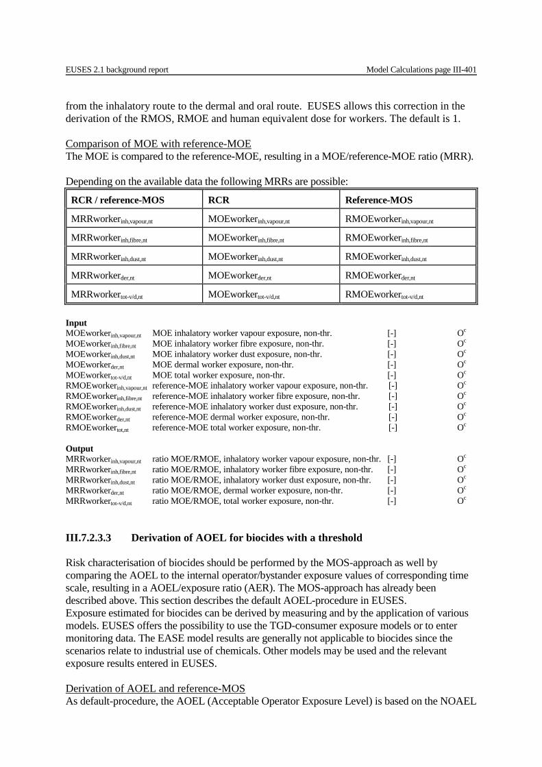
EUSES 2.1 background report Model Calculations page III-401
from the inhalatory route to the dermal and oral route. EUSES allows this correction in the derivation of the RMOS, RMOE and human equivalent dose for workers. The default is 1. Comparison of MOE with reference-MOE The MOE is compared to the reference-MOE, resulting in a MOE/reference-MOE ratio (MRR). Depending on the available data the following MRRs are possible:
RCR / reference-MOS RCR Reference-MOS
MRRworkerinh,vapour,nt MOEworkerinh,vapour,nt RMOEworkerinh,vapour,nt
MRRworkerinh,fibre,nt MOEworkerinh,fibre,nt RMOEworkerinh,fibre,nt
MRRworkerinh,dust,nt MOEworkerinh,dust,nt RMOEworkerinh,dust,nt
MRRworkerder,nt MOEworkerder,nt RMOEworkerder,nt
MRRworkertot-v/d,nt MOEworkertot-v/d,nt RMOEworkertot-v/d,nt
Input MOEworkerinh,vapour,nt MOE inhalatory worker vapour exposure, non-thr. [-] Oc MOEworkerinh,fibre,nt MOE inhalatory worker fibre exposure, non-thr. [-] Oc MOEworkerinh,dust,nt MOE inhalatory worker dust exposure, non-thr. [-] Oc MOEworkerder,nt MOE dermal worker exposure, non-thr. [-] Oc MOEworkertot-v/d,nt MOE total worker exposure, non-thr. [-] Oc RMOEworkerinh,vapour,nt reference-MOE inhalatory worker vapour exposure, non-thr. [-] Oc RMOEworkerinh,fibre,nt reference-MOE inhalatory worker fibre exposure, non-thr. [-] Oc RMOEworkerinh,dust,nt reference-MOE inhalatory worker dust exposure, non-thr. [-] Oc RMOEworkerder,nt reference-MOE dermal worker exposure, non-thr. [-] Oc RMOEworkertot,nt reference-MOE total worker exposure, non-thr. [-] Oc Output MRRworkerinh,vapour,nt ratio MOE/RMOE, inhalatory worker vapour exposure, non-thr. [-] Oc MRRworkerinh,fibre,nt ratio MOE/RMOE, inhalatory worker fibre exposure, non-thr. [-] Oc MRRworkerinh,dust,nt ratio MOE/RMOE, inhalatory worker dust exposure, non-thr. [-] Oc MRRworkerder,nt ratio MOE/RMOE, dermal worker exposure, non-thr. [-] Oc MRRworkertot-v/d,nt ratio MOE/RMOE, total worker exposure, non-thr. [-] Oc III.7.2.3.3 Derivation of AOEL for biocides with a threshold Risk characterisation of biocides should be performed by the MOS-approach as well by comparing the AOEL to the internal operator/bystander exposure values of corresponding time scale, resulting in a AOEL/exposure ratio (AER). The MOS-approach has already been described above. This section describes the default AOEL-procedure in EUSES. Exposure estimated for biocides can be derived by measuring and by the application of various models. EUSES offers the possibility to use the TGD-consumer exposure models or to enter monitoring data. The EASE model results are generally not applicable to biocides since the scenarios relate to industrial use of chemicals. Other models may be used and the relevant exposure results entered in EUSES. Derivation of AOEL and reference-MOS As default-procedure, the AOEL (Acceptable Operator Exposure Level) is based on the NOAEL
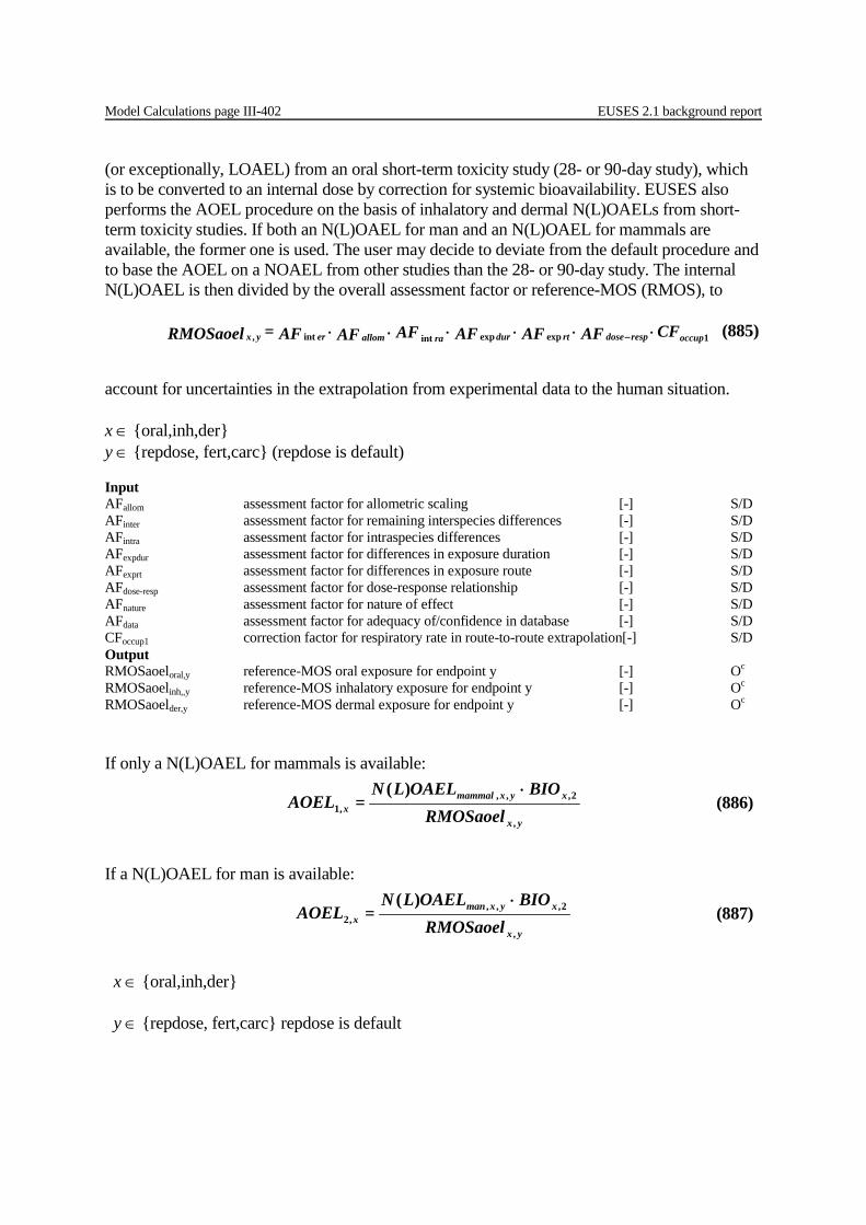
Model Calculations page III-402 EUSES 2.1 background report
(or exceptionally, LOAEL) from an oral short-term toxicity study (28- or 90-day study), which is to be converted to an internal dose by correction for systemic bioavailability. EUSES also performs the AOEL procedure on the basis of inhalatory and dermal N(L)OAELs from short-term toxicity studies. If both an N(L)OAEL for man and an N(L)OAEL for mammals are available, the former one is used. The user may decide to deviate from the default procedure and to base the AOEL on a NOAEL from other studies than the 28- or 90-day study. The internal N(L)OAEL is then divided by the overall assessment factor or reference-MOS (RMOS), to
account for uncertainties in the extrapolation from experimental data to the human situation. x ∈ {oral,inh,der} y ∈ {repdose, fert,carc} (repdose is default) Input AFallom assessment factor for allometric scaling [-] S/D AFinter assessment factor for remaining interspecies differences [-] S/D AFintra assessment factor for intraspecies differences [-] S/D AFexpdur assessment factor for differences in exposure duration [-] S/D AFexprt assessment factor for differences in exposure route [-] S/D AFdose-resp assessment factor for dose-response relationship [-] S/D AFnature assessment factor for nature of effect [-] S/D AFdata assessment factor for adequacy of/confidence in database [-] S/D CFoccup1 correction factor for respiratory rate in route-to-route extrapolation[-] S/D Output RMOSaoeloral,y reference-MOS oral exposure for endpoint y [-] Oc
RMOSaoelinh,,y reference-MOS inhalatory exposure for endpoint y [-] Oc
RMOSaoelder,y reference-MOS dermal exposure for endpoint y [-] Oc
If only a N(L)OAEL for mammals is available:
If a N(L)OAEL for man is available:
CF AF AF AF AF AF AF= RMOSaoel occuprespdosertdurallom raeryx 1expexpintint, ⋅⋅⋅⋅⋅⋅ − (885)
yx
xyxmammalx RMOSaoel
BIOOAELLN= AOEL
,
2,,,,1
)( ⋅ (886)
yx
xyxmanx RMOSaoel
BIOOAELLN= AOEL
,
2,,,,2
)( ⋅ (887)
x ∈ {oral,inh,der} y ∈ {repdose, fert,carc} repdose is default
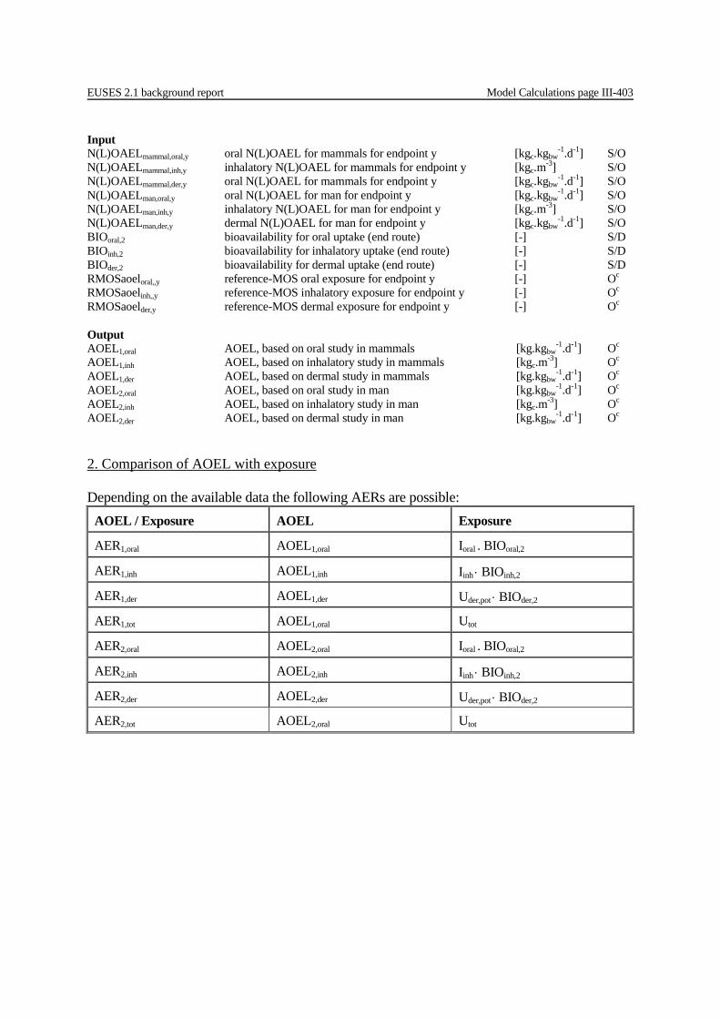
EUSES 2.1 background report Model Calculations page III-403
Input N(L)OAELmammal,oral,y oral N(L)OAEL for mammals for endpoint y [kgc.kgbw
-1.d-1] S/O N(L)OAELmammal,inh,y inhalatory N(L)OAEL for mammals for endpoint y [kgc.m-3] S/O N(L)OAELmammal,der,y oral N(L)OAEL for mammals for endpoint y [kgc.kgbw
-1.d-1] S/O N(L)OAELman,oral,y oral N(L)OAEL for man for endpoint y [kgc.kgbw
-1.d-1] S/O N(L)OAELman,inh,y inhalatory N(L)OAEL for man for endpoint y [kgc.m-3] S/O N(L)OAELman,der,y dermal N(L)OAEL for man for endpoint y [kgc.kgbw
-1.d-1] S/O BIOoral,2 bioavailability for oral uptake (end route) [-] S/D BIOinh,2 bioavailability for inhalatory uptake (end route) [-] S/D BIOder,2 bioavailability for dermal uptake (end route) [-] S/D RMOSaoeloral,,y reference-MOS oral exposure for endpoint y [-] Oc
RMOSaoelinh,,y reference-MOS inhalatory exposure for endpoint y [-] Oc
RMOSaoelder,y reference-MOS dermal exposure for endpoint y [-] Oc
Output AOEL1,oral AOEL, based on oral study in mammals [kg.kgbw
-1.d-1] Oc AOEL1,inh AOEL, based on inhalatory study in mammals [kgc.m-3] Oc AOEL1,der AOEL, based on dermal study in mammals [kg.kgbw
-1.d-1] Oc AOEL2,oral AOEL, based on oral study in man [kg.kgbw
-1.d-1] Oc AOEL2,inh AOEL, based on inhalatory study in man [kgc.m-3] Oc AOEL2,der AOEL, based on dermal study in man [kg.kgbw
-1.d-1] Oc 2. Comparison of AOEL with exposure Depending on the available data the following AERs are possible:
AOEL / Exposure AOEL Exposure
AER1,oral AOEL1,oral Ioral . BIOoral,2
AER1,inh AOEL1,inh Iinh ⋅ BIOinh,2
AER1,der AOEL1,der Uder,pot ⋅ BIOder,2
AER1,tot AOEL1,oral Utot
AER2,oral AOEL2,oral Ioral . BIOoral,2
AER2,inh AOEL2,inh Iinh ⋅ BIOinh,2
AER2,der AOEL2,der Uder,pot ⋅ BIOder,2
AER2,tot AOEL2,oral Utot
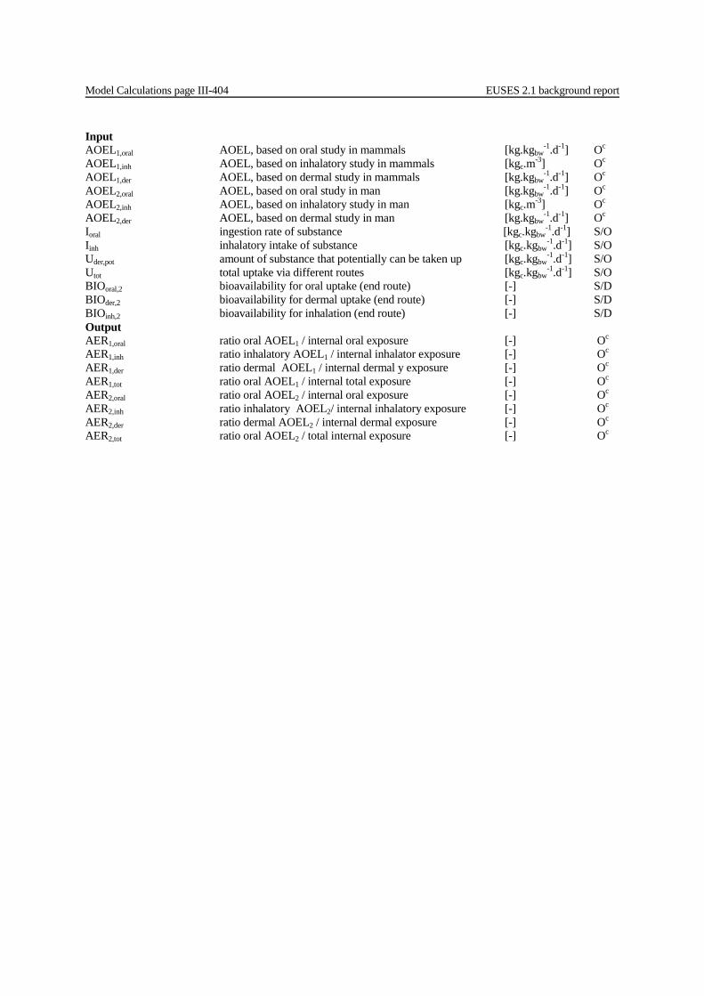
Model Calculations page III-404 EUSES 2.1 background report
Input AOEL1,oral AOEL, based on oral study in mammals [kg.kgbw
-1.d-1] Oc AOEL1,inh AOEL, based on inhalatory study in mammals [kgc.m-3] Oc AOEL1,der AOEL, based on dermal study in mammals [kg.kgbw
-1.d-1] Oc AOEL2,oral AOEL, based on oral study in man [kg.kgbw
-1.d-1] Oc AOEL2,inh AOEL, based on inhalatory study in man [kgc.m-3] Oc AOEL2,der AOEL, based on dermal study in man [kg.kgbw
-1.d-1] Oc Ioral ingestion rate of substance [kgc.kgbw
-1.d-1] S/O Iinh inhalatory intake of substance [kgc.kgbw
-1.d-1] S/O Uder,pot amount of substance that potentially can be taken up [kgc.kgbw
-1.d-1] S/O Utot total uptake via different routes [kgc.kgbw
-1.d-1] S/O BIOoral,2 bioavailability for oral uptake (end route) [-] S/D BIOder,2 bioavailability for dermal uptake (end route) [-] S/D BIOinh,2 bioavailability for inhalation (end route) [-] S/D Output AER1,oral ratio oral AOEL1 / internal oral exposure [-] Oc AER1,inh ratio inhalatory AOEL1 / internal inhalator exposure [-] Oc AER1,der ratio dermal AOEL1 / internal dermal y exposure [-] Oc AER1,tot ratio oral AOEL1 / internal total exposure [-] Oc AER2,oral ratio oral AOEL2 / internal oral exposure [-] Oc AER2,inh ratio inhalatory AOEL2/ internal inhalatory exposure [-] Oc AER2,der ratio dermal AOEL2 / internal dermal exposure [-] Oc AER2,tot ratio oral AOEL2 / total internal exposure [-] Oc

EUSES 2.1 background report Model Calculations page III-405
III.8 HYDROCARBON BLOCK METHOD (HBM) The principal steps in the application of the Hydrocarbon Block Method (HBM) are: • obtain compositional data for the substance that are sufficient to assign components to
blocks; • define blocks by grouping components on the basis of similar structural and/or physico-
chemical and ecotoxicological properties. If desired, blocks can be defined as single components;
• obtain production and use data; • establish release estimates for each block. A single release estimate for a petroleum
substance may not always be adequate; blocks with markedly different physico-chemical properties may require different release estimates;
• assign representative values for physico-chemical properties, degradation-rate constants and LC/EC50s and NOECs to each block;
• determine the PEC for each compartment for each block (local as well as regional); • determine the PNEC for each block; • calculate the PEC/PNEC ratio for each block, and sum. Once the blocks with their physico-chemical and ecotoxicological properties have been defined, the assessment follows the methods described in the following sections. This means that local and regional PECs can be calculated as described in the 'Environmental distribution module' and a PNEC can be derived as described in the 'Effects assessment module'.
Model Calculations page III-406 EUSES 2.1 background report
III.9 ENVIRONMENTAL RISK ASSESSMENT FOR METALS AND METAL COMPOUNDS
In principle, the models and approaches for organic substances can also be used to estimate exposure to metals. However, there are several differences compared with the use of these models for organic substances. Below, the differences are described. III.9.1 Exposure assessment 1. Physico-chemical properties (Input module) In general, water solubility, boiling point and vapour pressure cannot be used. The octanol-water partition coefficient is not appropriate and measured partition coefficients (Kp) should be used instead. 2. Partition coefficients (Environmental distribution module, partition coefficients sub-
module) Adsorption to aerosol particles Most of the metal present in the atmosphere will be bound to aerosols. Therefore, an extremely low value for the vapour pressure should be used to estimate the fraction bound to aerosol, e.g. 10-20 Pa. This leads to a value for Fassaer almost equal to one. If a valid measured value is available for the aerosol-bound fraction, this value can be used. Volatilisation Volatilisation can be ignored for metals, except for mercury compounds and several organometallo-compounds. Therefore, the Henry coefficient should generally be set to a very low value. Adsorption/desorption Formulae to estimate Koc cannot be used. Measured Kp-values must be used for water-soil, water-sediment and water-suspended matter. Kp is influenced by speciation and the speciation behaviour must therefore be accounted for in Kp. 3. Biotic and abiotic degradation rates (Environmental distribution module, Environmental
degradation rates sub-module) Not relevant for metals. The substances must be specified as non-biodegradable (very high DT50). 4. Elimination processes prior to the release in the environment (Environmental
distribution module, Sewage treatment sub-module) For applying the STP model, a partition coefficient is used for water-sludge. For metals, a measured Kp-value must be used. 5. Calculation of the regional PEC (Environmental distribution module, Regional
environmental distribution sub-module) The values applied for model parameters for the regional model, inter-media mass-transfer coefficients and model parameters for the continental concentration can be used.

EUSES 2.1 background report Model Calculations page III-407
III.9.2 Effects assessment PNECs can be derived through the application of assessment factors on the basis of the available data. Evaluation of the toxicity data is critical (the reader is referred to the TGD; EC, 1996). Standard methods applied for organic compounds can be used for this (see Section III.6). However, because of the specific mode of action that metals may have for some species, care should be taken in extrapolating short term toxicity data to the PNEC using the standard assessment factors. For many metals, sufficient long term toxicity data for aquatic organisms may be present to enable statistical extrapolation, results of which can support the results of PNECs calculated using assessment factors. Calculated PNECs derived for essential metals may not be lower than natural background concentrations. A prerequisite for the derivation of the PNEC is that it is done on the basis of the same level of availability as in exposure assessment: • Results from aquatic toxicity tests are usually expressed as total concentrations. As a first
approach, total concentrations have to be recalculated to dissolved concentrations using partition coefficients. If this is not possible, the total concentration can be set equal to the dissolved concentration. Differences in test systems, e.g. (semi-)static versus continuous flow systems and natural versus standard water, have to be considered.
• For the terrestrial compartment, many data exist, but most are only expressed as total concentration that has been added to the test media. This added amount will be partitioned among the aqueous and the solid phase. Application of partition coefficients to calculate the available concentration in soil can be applied. Soil type correction, using reference lines, should be applied to correct for differences among soil types (Slooff, 1992).
• Some of the metals are essential metals, having a function in biological processes at low concentrations. Shortage of micronutrients may cause malfunction. This implies that in setting the PNEC, information on deficiency levels should be taken into account. It should, however, be noted that often no information on deficiency levels of various metals for various species is available.
Though some exceptions exist, in general ionic metal species are considered to be the dominant metal species taken up, and are thus considered to be the metal species responsible for the toxic effect. Data on the concentration of ionic species in aquatic and terrestrial systems are not readily available, and cannot, as yet, be applied on a regular basis in risk assessment. Bioaccumulation of essential metals Metals are taken up by organisms. For essential metals, biota regulate their uptake by means of the general physiological mechanism of homeostasis. By this mechanism, organisms will keep, within a certain range of varying external concentrations, their intracellular levels relatively constant, in order to satisfy their requirements for that essential element. Homeostasis implies that organisms can actively concentrate essential elements if concentrations in the environment are very low. This may lead to high BCF values. On the other hand, the homeostatic regulation capacity will be exceeded at a given higher external concentration beyond which the element will accumulate and become toxic.