handbook for calculations of nuclear reaction data, ripl-2 · pdf filehandbook for...

IAEA-TECDOC-1506

Handbook for calculations ofnuclear reaction data, RIPL-2

Reference Input Parameter Library-2

Final report of a coordinated research project

August 2006

The originating Section of this publication in the IAEA was:

Nuclear Data Section International Atomic Energy Agency

Wagramer Strasse 5 P.O. Box 100

A-1400 Vienna, Austria

HANDBOOK FOR CALCULATIONS OF NUCLEAR REACTION DATA, RIPL-2 IAEA, VIENNA, 2006 IAEA-TECDOC-1506 ISBN 92–0–105206–5

ISSN 1011–4289 © IAEA, 2006

Printed by the IAEA in Austria August 2006

FOREWORD

Nuclear data for applications constitute an integral part of the IAEA programme of ac-tivities. When considering low-energy nuclear reactions induced with light particles, suchas neutrons, protons, deuterons, alphas and photons, a broad range of applications areaddressed, from nuclear power reactors and shielding design through cyclotron productionof medical radioisotopes and radiotherapy to transmutation of nuclear waste. All theseand many other applications require a detailed knowledge of production cross sections,spectra of emitted particles and their angular distributions.

A long-standing problem of how to meet the nuclear data needs of the future withlimited experimental resources puts a considerable demand upon nuclear model compu-tation capabilities. Originally, almost all nuclear data were provided by measurementprogrammes. Over time, theoretical understanding of nuclear phenomena has reached ahigh degree of reliability, and nuclear modeling has become standard practice in nucleardata evaluations (with measurements remaining critical for data testing and benchmark-ing). Thus, theoretical calculations are instrumental in obtaining complete and internallyconsistent nuclear data files.

The practical use of nuclear model codes requires a considerable numerical input thatdescribes the properties of the nuclei and the interactions involved. Experts have useda variety of different input sets, often developed over years in their own laboratories.Many of these partial input databases were poorly documented or not documented atall, and were not always available for other users. With the trend of reduced funds fornuclear data evaluations, there is a real threat that the immense accumulated knowledgeof input parameters and associated calculations may be compromised or even lost forfuture applications. Therefore, the IAEA has undertaken an extensive co-ordinated effortto develop a library of evaluated and tested nuclear-model input parameters.

Considering that such a task is so immense, it was decided to proceed in two majorsteps. First, to summarize the present knowledge on input parameters and to develop asingle Starter File of input model parameters, and then to focus on testing, validating andimproving the Starter File. The first step was addressed through the IAEA Co-ordinatedResearch Project (CRP) entitled “Development of Reference Input Parameter Library forNuclear Model Calculations of Nuclear Data (Phase I: Starter File)”, initiated in 1994and completed successfully in 1997. The electronic Starter File (known as RIPL-1) wasdeveloped and made available to users throughout the world. The second step followedimmediately afterwards within the CRP entitled “Nuclear Model Parameter Testing forNuclear Data Evaluation (Reference Input Parameter Library: Phase II)”, initiated in1998 and completed in 2002. This later CRP resulted in the revision and extension ofthe original RIPL-1 Starter File to produce a consistent RIPL-2 library containing rec-ommended input parameters, a large amount of theoretical results suitable for nuclearreaction calculations, and a number of computer codes for parameter retrieval, determi-nation and use. The new library will be of immediate practical value for a number ofusers and should represent a firm basis for future improvements.

Initial objectives of the RIPL-2 CRP were:

• Test and improve nuclear model parameters for theoretical calculations of nuclearreaction cross sections at incident energies below 100 MeV.

• Produce a well-tested Reference Input Parameter Library for calculations of nuclearreactions using nuclear reaction codes.

• Develop user-oriented retrieval tools and interfaces to established codes for nuclearreaction calculations.

• Publish Technical Report and make the library and tools available on-line and onCD-ROM.

The CRP participants (T. Belgya (Hungary), O. Bersillon (France), R. Capote Noy(Cuba), T. Fukahori (Japan), Ge Zhigang (China), S. Goriely (Belgium), M. Herman(IAEA), A. V. Ignatyuk (Russian Federation), S. Kailas (India), A. J. Koning (Nether-lands), P. Oblozinsky (USA), V. Plujko (Ukraine) and P. G. Young (USA)) convened atthree Research Co-ordination Meetings held at:

• Vienna, Austria, 25-27 November 1998 (see INDC(NDS)-389, February 1999)

• Varenna, Italy, 12-16 June 2000 (see INDC(NDS)-416, September 2000)

• Vienna, Austria, 3-7 December 2001 (see INDC(NDS)-431, April 2002)

to discuss progress and agree on the contents and form of the new library. In the courseof work, the original scope of the CRP has been substantially extended by inclusion ofnew quantities and results of microscopic calculations for about 8000 nuclei. Extensiveefforts have also been dedicated to the testing of the RIPL-2 data.

RIPL-2 is targeted at users of nuclear reaction codes interested in low-energy nuclearapplications. Incident and outgoing particles include neutrons, protons, deuterons, tri-tons, 3He, 4He and γ, with energies up to approximately 100 MeV. The numerical dataand computer codes included in the library are arranged in seven segments/directories:

No Directory Contents

__ _________ ____________________________________

1 MASSES Atomic Masses and Deformations

2 LEVELS Discrete Level Schemes

3 RESONANCES Average Neutron Resonance Parameters

4 OPTICAL Optical Model Parameters

5 DENSITIES Level Densities (Total, Partial)

6 GAMMA Gamma-Ray Strength Functions

7 FISSION Fission Barriers and Level Densities

The RIPL-2 library is physically located at a Web server operated by the IAEA, andcan be conveniently accessed by pointing any Web browser at:

http://www-nds.iaea.org/RIPL-2/This Web site provides for downloading entire RIPL-2 segments, individual files, andretrieval of selected data. In addition, some basic calculations and graphical comparisonsof parameters are also available. A CD-ROM with the complete RIPL-2 library canbe requested cost-free from the IAEA. This Handbook contains a full description of thelibrary including the physics involved, with an introductory and seven technical chapters,plus related Annexes that describe the library structure as defined above.

During the development of RIPL-2, several important issues could not be addressedwithin the current CRP. Therefore, a third phase of the RIPL project has been initiatedin 2002 in order to extend the applicability of the library to cross sections for reactionson nuclei far from the stability line, incident energies beyond 100 MeV, and reactionsinduced by charged particles. This phase is planned for completion in 2006-07.

The IAEA wishes to thank all participants of the CRP for their diligent work thathas lead to the creation of the Reference Input Parameter Library, and for their valu-able contributions to the present Technical Report. Finally, M. Herman was the IAEAresponsible officer for the CRP, this publication and the resulting database.

EDITORIAL NOTE

The use of particular designations of countries or territories does not imply any judgement by the publisher, the IAEA, as to the legal status of such countries or territories, of their authorities and institutions or of the delimitation of their boundaries.

The mention of names of specific companies or products (whether or not indicated as registered) does not imply any intention to infringe proprietary rights, nor should it be construed as an endorsement or recommendation on the part of the IAEA.

T. Belgya (Institute of Isotope and Surface Chemistry, Hungary)O. Bersillon (Centre d’Etudes Nucleaires de Bruyeres-le-Chatel, France)R. Capote Noy (Centro de Estudios Aplicados al Desarrollo Nuclear, Cuba)T. Fukahori (Japan Atomic Energy Agency, Japan)Ge Zhigang (China Institute of Atomic Energy, China)S. Goriely (Universite Libre de Bruxelles, Belgium)M. Herman (International Atomic Energy AgencyA.V. Ignatyuk (Institute of Physics and Power Engineering, Russian Federation)S. Kailas (Bhabha Atomic Research Centre, India)A.J. Koning Netherlands)P. Oblozinsky (Brookhaven National Laboratory, USA)V. Plujko (Taras Shevchenko National University, Ukraine)P.G. Young (Los Alamos National Laboratory, USA)

Contributing Authors

)

Nuclear Resear and Consultanc Group,ych(

r

Contents

1 Introduction 1

2 Atomic Masses 5

2.1 Atomic masses . . . . . . . . . . . . . . . . . . . . . . . . . . . . . . . . . 5

2.1.1 Experimental masses . . . . . . . . . . . . . . . . . . . . . . . . . . 6

2.1.2 Finite-Range-Droplet-Model mass table . . . . . . . . . . . . . . . . 6

2.1.3 Hartree-Fock-Bogoliubov mass table . . . . . . . . . . . . . . . . . 6

2.1.4 Duflo-Zuker approximation to the Shell Model . . . . . . . . . . . . 7

2.2 Shell corrections . . . . . . . . . . . . . . . . . . . . . . . . . . . . . . . . . 8

2.3 Deformations . . . . . . . . . . . . . . . . . . . . . . . . . . . . . . . . . . 9

2.4 Relative isotopic abundances . . . . . . . . . . . . . . . . . . . . . . . . . . 9

2.5 Summary of codes and data files . . . . . . . . . . . . . . . . . . . . . . . . 9

3 Discrete Levels 11

3.1 Discrete Level Scheme Library (DLSL) . . . . . . . . . . . . . . . . . . . . 12

3.1.1 Format of the Discrete Level Schemes Library . . . . . . . . . . . . 14

3.1.2 Conventions and methods . . . . . . . . . . . . . . . . . . . . . . . 16

3.1.3 Format of the file with constant-temperature fit parameters . . . . 17

3.2 Applied procedures . . . . . . . . . . . . . . . . . . . . . . . . . . . . . . . 19

3.2.1 Construction of Discrete Level Scheme Library . . . . . . . . . . . 19

3.2.2 Consistency tests . . . . . . . . . . . . . . . . . . . . . . . . . . . . 21

3.2.3 Physical validation of the files . . . . . . . . . . . . . . . . . . . . . 24

Annex 3.A Procedure for Constant Temperature Fittingof Cumulative Number of Levels . . . . . . . . . . . . . . . . . . . 27

Annex 3.B Determination of Unique Spins . . . . . . . . . . . . . . . . . . . . 29

Annex 3.C Determination of Missing Internal Conversion Coefficients . . . . . 31

Annex 3.D Calculation of Decay Probabilities . . . . . . . . . . . . . . . . . . . 32

Annex 3.E Simple Method for Determination of ApproximateNuclear Temperature . . . . . . . . . . . . . . . . . . . . . . . . . . 33

Annex 3.F Flowchart of DLSL Construction . . . . . . . . . . . . . . . . . . . 34

4 Average Neutron Resonance Parameters 37

4.1 Evaluation methods . . . . . . . . . . . . . . . . . . . . . . . . . . . . . . . 38

4.2 Files of average neutron resonance parameters . . . . . . . . . . . . . . . . 40

4.3 Conclusions and recommendations . . . . . . . . . . . . . . . . . . . . . . . 45

5 Optical Model Parameters 47

5.1 Phenomenological parameterizations . . . . . . . . . . . . . . . . . . . . . 48

5.1.1 Description of the potential . . . . . . . . . . . . . . . . . . . . . . 48

5.1.2 Dispersive relations . . . . . . . . . . . . . . . . . . . . . . . . . . . 49

5.1.3 Nucleon-nucleus potentials . . . . . . . . . . . . . . . . . . . . . . . 49

5.1.4 Complex-particle potentials . . . . . . . . . . . . . . . . . . . . . . 51

5.1.5 Format of OMP library . . . . . . . . . . . . . . . . . . . . . . . . . 52

5.1.6 Contents of OMP library . . . . . . . . . . . . . . . . . . . . . . . . 53

5.2 Microscopic optical model . . . . . . . . . . . . . . . . . . . . . . . . . . . 54

5.3 Validation . . . . . . . . . . . . . . . . . . . . . . . . . . . . . . . . . . . . 54

5.4 Recommendations and conclusions . . . . . . . . . . . . . . . . . . . . . . 56

5.4.1 Recommendations . . . . . . . . . . . . . . . . . . . . . . . . . . . . 56

5.4.2 Conclusions . . . . . . . . . . . . . . . . . . . . . . . . . . . . . . . 58


Annex 5.A Optical Model Parameter Format for RIPL Library . . . . . . . . . 65

Annex 5.B Reference Numbering System for RIPL OpticalModel Potentials . . . . . . . . . . . . . . . . . . . . . . . . . . . . 69

Annex 5.C Example of a Potential in the Optical Parameter Library . . . . . . 70

Annex 5.D Summary of Entries and References Included in the RIPL-2Optical Model Potential Library . . . . . . . . . . . . . . . . . . . . 72

6 Nuclear Level Densities 85

6.1 Total level densities . . . . . . . . . . . . . . . . . . . . . . . . . . . . . . . 86

6.1.1 Composite Gilbert-Cameron model . . . . . . . . . . . . . . . . . . 86

6.1.2 Back-shifted Fermi-gas model . . . . . . . . . . . . . . . . . . . . . 92

6.1.3 Generalized superfluid model . . . . . . . . . . . . . . . . . . . . . 98

6.1.4 Microscopic Generalized Superfluid Model . . . . . . . . . . . . . . 104

6.2 Partial level densities . . . . . . . . . . . . . . . . . . . . . . . . . . . . . . 106

6.2.1 Equidistant formula with exact Pauli correction term and binding-energy and well-depth restrictions . . . . . . . . . . . . . . . . . . . 107

6.2.2 Microscopic theory . . . . . . . . . . . . . . . . . . . . . . . . . . . 108



7 Gamma-Ray Strength Functions 117

7.1 Experimental γ-ray strength functions . . . . . . . . . . . . . . . . . . . . 118

7.2 Standard closed-form models for E1 strength function . . . . . . . . . . . . 119

7.3 Refined closed-form models for E1 strength function . . . . . . . . . . . . . 120

7.4 Comparison of closed-form expressions with experimental data . . . . . . . 124

7.5 Microscopic approach to E1 strength function . . . . . . . . . . . . . . . . 127

7.6 Giant dipole resonance parameters . . . . . . . . . . . . . . . . . . . . . . 129

7.7 M1 and E2 transitions . . . . . . . . . . . . . . . . . . . . . . . . . . . . . 132



8 Nuclear Fission 139

8.1 Fission barriers and level densities for pre-actinides . . . . . . . . . . . . . 140

8.2 Fission barriers and level densities for actinides . . . . . . . . . . . . . . . 143

8.3 Large-scale microscopic calculations of fission barriers and level densities . 148

8.3.1 Fission barriers . . . . . . . . . . . . . . . . . . . . . . . . . . . . . 149

8.3.2 Fission level densities . . . . . . . . . . . . . . . . . . . . . . . . . . 151



List of participants

157Errata

159

1 INTRODUCTION

An important trend in the evaluation of neutron and charged-particle nuclear data isthe increased use of nuclear reaction theory codes to compute cross sections, spectra andangular distributions required for a large variety of applications. As a matter of principle,the use of model codes offers many advantages such as preservation of the energy balanceand coherence of partial cross sections with total and/or reaction cross sections. Thesefeatures are essential for consistent and reliable transport calculations. In addition, thetheoretical approach permits the prediction of data for unstable nuclei and fills gaps inthe experimental data. Nuclear reaction theory is believed to be in a position to meetmany of the requirements for practical applications. The major sources of uncertainty arethe input parameters needed to perform theoretical calculations.

For any nuclear reaction calculation, nuclear masses are the basic data for obtainingbinding energies and Q-values. These data are presented in Chapter 2, together withother useful information such as ground state deformations.

Discrete level schemes, including spins, parities, γ-transition branchings and conver-sion coefficients are important for the determination of low-energy nuclear level densitiesand for cross-section calculations. Most of the related experimental information is con-tained in the ENSDF library. However, the format of the ENSDF library is not appropriatefor reaction calculations. In addition, a lack of unique spin and/or parity assignments formany levels, and missing conversion coefficients for most of the electromagnetic transitionsprevent direct use of the ENSDF library by the reaction model codes. To overcome thesedeficiencies, a dedicated RIPL-2 library of discrete levels has been created. Chapter 3describes the contents, along with the procedures used to retrieve the necessary data andfill gaps.

As is well known, neutron cross sections at low incident energies exhibit resonantbehavior, and a careful statistical analysis of the experimental results leads to the averageneutron resonance parameters, as described in Chapter 4. These average quantities arenot directly used in the model calculations, but are important data for constraining theparameters of different models:

• average spacing of resonances is the only measure of the level density near theneutron binding energy,

• neutron strength functions have to be reproduced by the optical model at low en-ergies, and

• average radiative width is used to normalize γ-ray strength functions.

Above the resonance energy region, the nuclear reaction models can only reproducethe smooth behavior of the cross sections, and the evaluation of nuclear data is generallydivided into two major steps. By using the optical model in the first step, the elasticchannel and the direct inelastic channels for deformed nuclei are explicitly calculated,whereas all other channels are lumped together in the reaction cross section. Chapter 5gives an extensive compilation of optical model parameters for different types of incident

1

particles, from the neutron to 4He. A consistent evaluation can be achieved for eachinteracting system by using a unique parameterization which reproduces the relevant ob-servables (total or reaction cross sections, elastic angular distributions, analyzing powers)over an energy range as broad as possible, including, the low energy region in the caseof neutron interaction, where the calculated neutron strength function and scattering ra-dius should match the experimental values. Furthermore, the parameters should have asmooth energy dependence.

The second step consists in sharing the reaction cross section among all possible indi-vidual channels. For incident energies lower than about 10 MeV, this is done by using thestatistical decay of the compound nucleus, a formalism often referred to as the Hauser-Feshbach theory. Written in a compact form, the Hauser-Feshbach formula that gives thecross section for the A(a,b)B reaction is represented by the expression:

σa→b =∑Jπ

Ta Tb∑i

∑c Tic

where the index i stands for the different types of outgoing particles1 (or the fissionchannel, if any), and the T s are the transmission coefficients calculated by the opticalmodel for this particle. The index c represents all accessible final states which are eitherdiscrete excited levels of the residual nucleus or a continuum of levels described by thelevel density.

In the case of discrete levels, one should only take into account the low-lying levels ofknown excitation energy, spin, parity, and decay branchings (if γ production is required).Above the energy of the last level for which one of the previous quantities is missing oruncertain, one has to consider a continuum of levels described by the total level density.At low excitation energy, the level density should match the cumulative number of discretelevels and reproduce the average spacing of neutron resonances at the neutron bindingenergy. Different theoretical approaches to this longstanding problem are presented inSection 6.1.

For incident energies higher than approximately 10 MeV, the pre-equilibrium reactionmechanism constitutes the bridge between fast (direct) processes and slow (compound)processes providing for the high-energy tails in spectra and the smoothly forward peakedangular distributions. Methods for calculating partial (or particle-hole) level densitiesused in the pre-equilibrium model calculations are given in Section 6.2.

Gamma-ray emission is an almost universal reaction channel since γ rays, in general,accompany any nuclear reaction. Modeling of the γ cascade provides γ spectra and allowscalculation of isomeric cross sections. The basic quantity is the γ-ray strength functionderived typically from the Giant Resonance parameters, as discussed in Chapter 7.

The fission cross-section calculations depend on two key ingredients: (i) fission leveldensity (level density of the fissioning nucleus at the saddle point deformation), and (ii)fission barriers. These two strongly interdependent parameters are discussed in Chap-ter 8.

1Outgoing particles considered are normally p, n, d, t, 3He, α and γ.

2

Many of the parameters are model dependent, and should therefore be used strictlywithin the frame of their definitions. Although the parameters reported in RIPL-2 areready to be used in reaction calculations, some of them may still need improvements or ad-justments. The reaction models are particularly sensitive to optical model potentials andtotal level densities, which have to reproduce consistently different pieces of information.Therefore, utmost care should be applied when selecting an adequate set of parameters.

Due to the extensive testing and additions, the RIPL-2 database has been substantiallyimproved compared to the original RIPL-1 database. Nevertheless, RIPL-2 does not fullysupersede the original RIPL-1 library since only the recommended files were consideredin the RIPL-2 exercise. So called ‘other’ files of RIPL-1 were not incorporated in thenew database. Although these do not match the level of testing typical for RIPL-2, theystill might be of practical use in nuclear data evaluations or basic research, and thereforeRIPL-1 information and data continue to be fully tracable through:

(a) Handbook for Calculations of Nuclear Reaction Data - Reference Input ParameterLibrary, IAEA-TECDOC-1034, IAEA, Vienna (1998);

(b) Web site address: http://www-nds.iaea.org/ripl/;

(c) CD-ROM: RIPL-1.

RIPL-2 contains numerical values for most of the parameters needed to model nuclearreactions and a number of computer codes. For nuclei close to the stability line, theparameters were derived from the available experimental data. For a certain nucleus,these are usually sets of a few numbers used by the reaction codes to calculate derivedquantities such as Q-values, transmission coefficients, level densities or γ-ray strengthfunctions. Often, these parameters are supplemented with closed-form systematics to fillgaps in the experimental data. Since these systematics were obtained by fitting existingdata, their extrapolation to the nuclei far from the stability line is doubtful. Therefore,RIPL-2 also contains parameters and some derived quantities provided by the large-scalecalculations within microscopic models adjusted to the existing experimental data. Theseresults are tabulated for practically all nuclei between drip lines and can be directly usedby nuclear reaction codes. All RIPL-2 data are stored in a unified format to facilitatetheir use. In addition to the model parameters, RIPL-2 includes a number of utilitycodes, which are intended for calculating derived quantities from the RIPL-2 parameters,data retrieval and library maintenance. The internet address for the RIPL-2 database ishttp://www-nds.iaea.org/RIPL-2/.

3

2 ATOMIC MASSES

Coordinator: S. Goriely

Summary

Nuclear ground state properties are fundamental quantities in many different fields ofphysics. The present chapter considers the available experimental data concerning theatomic masses (Audi and Wapstra 1995 [2.1]), as well as the deformation parameters(Raman et al. 2001 [2.13]) extracted from the experimental reduced electric quadrupoletransition probability. When no experimental data exist, ground-state properties canbe derived from local or global theoretical approaches. RIPL-2 provides ground-stateproperties predicted by three global models: the Finite-Range Droplet Model (Moller etal. 1995 [2.3]), the Hartree-Fock-Bogoliubov Model (Goriely et al. 2002 [2.6]) and theapproximation to the Shell Model by Duflo and Zuker (1995 [2.8]). In addition to nu-clear masses, the FRDM model also provides microscopic corrections and deformationparameters, while the HFB model provides density distributions and deformation param-eters. Relative isotopic abundances for all stable nuclei found naturally on earth are alsoprovided as supplementary information.

2.1 Atomic masses

Nuclear ground state properties, and more particularly nuclear masses, are fundamentalquantities in many different fields of physics. The mass Mnuc(N, Z) of a nucleus with Nneutrons (of mass Mn) and Z protons (of mass Mp) is measurably different from the sumof the masses of the free nucleons, and provides a direct determination of the internalenergy Enuc (negative of the binding energy) of the nucleus:

Enuc = {Mnuc(N, Z) −NMn − ZMp}c2 (2.1)

The atomic mass can be calculated from the nuclear mass from the relationship:

Mat = Mnuc(N, Z) + ZMe − Be(Z) (2.2)

where Me is the electron mass, and Be is the total atomic binding energy of all electrons.

Most of the nuclear masses for nuclei close to the stability line were measured with highaccuracy. However, many applications involve nuclear species for which no experimentaldata are available. In these cases, they have to be estimated on a theoretical basis.Many different mass formulae are available nowadays. We will consider here only globalapproaches, which provide predictions of nuclear masses for all nuclei lying between theproton and the neutron drip lines up to the super-heavy region Z <∼ 120.

5

2.1.1 Experimental masses

The latest compilation of experimental atomic masses at the time was the 1995 workof Audi and Wapstra [2.1], which includes 1964 nuclei. In addition, these authors alsoestimated a set of additional 967 masses from trends in systematics based on the regularityof the mass surface. This final set of Audi and Wapstra best recommended masses included2931 nuclei.

2.1.2 Finite-Range-Droplet-Model mass table

Attempts to develop formula or algorithms representing the variation in Enuc from onenucleus to another go back to the 1935 “semi-empirical mass formula” of von Weizsacker[2.2]. This approach corresponds to the widely used liquid-drop model of the nucleus,i.e., the macroscopic mass formula which accounts for all but a small part of the vari-ation in the binding energy. Improvements have been gradually made to the originalliquid-drop mass formula, leading to the development of macroscopic-microscopic massformulae, where microscopic corrections accounting for the shell and pairing correlationeffects are added to the liquid drop part. Thus, the macroscopic and microscopic fea-tures are treated independently, both parts being connected exclusively by a parameterfit to experimental masses. Later developments included modifications to the macroscopicproperties of the infinite and semi-infinite nuclear matter and the finite range character ofthe nuclear forces. The most sophisticated version of this macroscopic-microscopic massformula is the “finite-range droplet model” (FRDM) [2.3]. The atomic mass excessesand nuclear ground-state deformations are tabulated for 8979 nuclei ranging from 16O toA=339. The calculations are based on the finite-range droplet macroscopic model and thefolded-Yukawa single-particle microscopic correction. Relative to the 1981 version, im-provements are mainly found in the macroscopic model, pairing model with a new formfor the effective-interaction pairing gap, and minimization of the ground-state energy withrespect to the additional shape degrees of freedom. The parameters are determined di-rectly from a least-squares adjustment to the ground-state masses of 1654 nuclei rangingfrom 16O to 106Sg. The error of this mass model is 0.689 MeV for the 1888 Z, N ≥ 8nuclei with experimental masses. Data file mass-frdm95.dat includes the Audi andWapstra (1995) experimental and best recommended masses when available, along withthe FRDM calculated masses, microscopic corrections and deformation parameters inthe β-parameterization. The microscopic correction Emic corresponds to the differencebetween the total binding energy and the spherical macroscopic energy (see below).

2.1.3 Hartree-Fock-Bogoliubov mass table

As well as the liquid-drop approach, there are microscopic theories based on the nucleonicinteractions providing estimates of the binding energies. The most promising approachnowadays is the non-relativistic Hartree-Fock (HF) method based on an effective nucleon-nucleon interaction of Skyrme type. It was demonstrated that HF calculations in whichthe Skyrme force is fitted essentially to all mass data are not only feasible, but can alsocompete with the most accurate droplet-like formulae available nowadays [2.4].

6

Recently, a new Skyrme force has been derived on the basis of HF calculations withpairing correlations taken into account in the Bogoliubov approach, using a δ-functionpairing force [2.5, 2.6]. Pairing correlations are often described within the BCS framework.However, the BCS procedure neglects the fact that the scattering of nucleon pairs betweendifferent single-particle states under the influence of the pairing interaction will actuallymodify the single-particle states, a difficulty that becomes particularly serious close to theneutron-drip line where nucleon pairs are scattered into the continuum. For such nuclei,this problem is avoided in the HF-Bogoliubov (HFB) method.

The Skyrme and pairing parameters of the HFB-2 mass table are determined by fittingto all Audi and Wapstra (1995) experimental masses for 1888 Z, N ≥ 8 nuclei, bothspherical and deformed. A Wigner correction term of the form EW = VW exp(−λ(N −Z)2/A2)−V ′

W |N −Z| exp(−A2/A20) is also included to account for the over-binding in the

Z � N nuclei. The latest force (BSk2) is a standard Skyrme which gives an rms error of0.680 MeV with respect to the 1888 known masses. The quality of the HFB predictionsis identical to the one obtained with the FRDM (the same rms of about 0.680 MeVon the same set of masses). The BSk2 force is characterized by the following nuclearmatter properties: energy per nucleon at equilibrium in symmetric nuclear matter av =−15.794 MeV, the corresponding density ρ0 = 0.1575 fm−3, the isoscalar effective massM∗

s /M = 1.04, the isovector effective mass M∗v /M = 0.86 and the symmetry coefficient

J = 28 MeV. Details regarding the BSk2 force can be found in Ref. [2.6] and thoseregarding the HFB model in Ref. [2.5]. The HFB model was also found to give reliablepredictions of nuclear radii. A comparison with the measured radii of the 523 nuclei inthe 1994 data compilation of Nadjakov et al. [2.7] shows an rms error of 0.028 fm.

The complete HFB-2 mass table is available in the mass-hfb02.dat file. In addi-tion to the Audi and Wapstra (1995) experimental and best recommended masses whenavailable, this mass table includes the HFB masses, deformation parameters in the β-parameterization and the parameters of the nucleon density distribution for all 9200 nucleilying between the two drip lines over the range Z, N ≥ 8 and Z ≤ 120. The density dis-tribution amplitude ρq,0, radius rq and diffuseness aq are determined by fitting the HFBdistribution by a simple spherical Fermi function ρq(r) = ρq,0/[1 + exp(−(r − rq)/aq)].Note that the amplitude ρq,0 is determined so that the nucleon number is conserved inthe spherical approximation. Exact HFB density distributions (assuming spherical sym-metry) are also tabulated in the matter-density-hfb02 subdirectory for nuclear radiiup to 15 fm in steps of 0.1 fm. The tabulated nucleon densities do not take into accountthe finite size of the proton.

2.1.4 Duflo-Zuker approximation to the Shell Model

Another microscopic approach worth considering is the development by Duflo and Zuker[2.8] of a mass formula based on the shell model. In this approach, the nuclear Hamiltonianis separated into a monopole term and a residual multipole term. The monopole term isresponsible for saturation and single-particle properties, and is fitted phenomenologically,while the multipole part is derived from realistic interactions. The latest version of themass formula made of 10 free parameters reproduces the 1888 Z, N ≥ 8 experimentalmasses with an rms error of 0.553 MeV. A simple 120-lines FORTRAN subroutine in themasses/duflo-zuker96.for file makes the computation of any mass straightforward, and

7

is especially useful when the nucleus is not available in the previously mentioned tables.

2.2 Shell corrections

The microscopic correction to the binding energy is a quantity of fundamental importancein the derivation of many physical properties affected by the shell, pairing and deformationeffects. However, there is a lot of confusion in the literature about what is referred to asthe shell correction energy; different definitions exist. The most common one defines thevarious microscopic corrections (e.g., [2.3]) as follows:

The total nuclear binding energy is written as

Etot(Z, A, β) = Emac(Z, A, β) + Es+p(Z, A, β) (2.3)

where β characterizes the nuclear shape at equilibrium, i.e., the shape which minimizesthe total binding energy. Es+p = Eshell +Epair is the shell-plus-pairing correction energy1.Defining a macroscopic deformation energy by the difference in the macroscopic energybetween the equilibrium and spherical shape:

Edef (Z, A, β) = Emac(Z, A, β)−Emac(Z, A, β = 0), (2.4)

the total nuclear binding energy can now be expressed as

Etot(Z, A, β) = Emac(Z, A, β = 0) + Emic(Z, A, β) (2.5)

with the microscopic correction

Emic(Z, A, β) = Eshell(Z, A, β) + Epair(Z, A, β) + Edef (Z, A, β) (2.6)

including all shell, pairing and deformation effects. Another frequent definition of themicroscopic energy considers the experimental energy Eexp(Z, A), when available, insteadof the total theoretical binding energy Etot and is given by the equation:

Eexpmic = Eexp(Z, A)− Emac(Z, A, β) (2.7)

� Eshell(Z, A, β) + Epair(Z, A, β) = Es+p(Z, A, β) (2.8)

Should the mass formula be exact, Eexpmic = Es+p(Z, A, β). Although Eexp

mic is often referredto as an “experimental” microscopic correction, this terminology is incorrect, since the pa-rameter remains model-dependent through the use of the model-dependent Emac quantity.Each mass model calls for specific theoretical backgrounds to estimate the macroscopicpart, as well as the shell, pairing and deformation energies. The most common approachesto derive the macroscopic part are the Finite-Range Droplet or Liquid Drop model [2.3],the Thomas-Fermi approach [2.9] or the Extended-Thomas-Fermi approach [2.10]. De-pending on the approach followed to derive the smooth macroscopic part of the bindingenergy and the parameter set adopted for the macroscopic part, the microscopic correc-tions can take different values. The FRDM microscopic correction Emic can be found inthe mass-frdm95.dat file. This dataset also contains the deformation corrections calcu-lated for the deformation parameters β2 and β4 estimated from the FRDM mass formula.

1Note that we define the pairing correction for even-even nuclei, and do not consider the odd-eveneffect also attributed to the pairing interaction.

8

Therefore, these corrections can also be used for transforming the FRDM microscopic cor-rections into the corresponding FRDM shell corrections. The shell corrections calculatedaccording to the liquid drop model of Myers-Swiatecki [2.11] are included in the “NuclearLevel Densities” segment (shellcor-ms.dat file).

When shell, pairing and deformation corrections are introduced to a given quantity(for example the nuclear level density) using the corresponding energy correction, specialattention should be paid to the prescription adopted. In particular, depending on the leveldensity formula considered, the ”microscopic” correction to the level density a-parametercan include very different effects, so that different energy corrections should be considered(see [2.12] for more details).

2.3 Deformations

In addition to the theoretical deformation parameters derived from the FRDM and HFBground-state predictions, information can also be extracted from the experimental reducedelectric quadrupole transition probabilities B(E2). Assuming a uniform charge distribu-tion to distance R and zero charge beyond, the model-dependent deformation parameterβ is related to B(E2) by [2.13]:

β =4π

3ZR20

[B(E2)/e2]2 (2.9)

where R0 = 1.2 A1/3. The final compilation of 328 experimental deformation parametersβ (and corresponding uncertainties) is included in the gs-deformations-exp.dat file.Note that a similar parameter β2 is widely used in the theory of the direct-interactionexcitation of collective states to describe the deformation of the average potential. Whilethe β values given here provide a useful guide to the values to be expected for this nuclearpotential deformation parameter, the β and β2 values can differ somewhat.

2.4 Relative isotopic abundances

For practical applications, the relative isotopic abundances (expressed in percent) foreach stable nucleus found naturally on earth is given in the abundance.dat file. Thedata originate from the Nuclear Wallet Cards, as retrieved from Brookhaven NationalLaboratory [2.14].

2.5 Summary of codes and data files

The programs and data files included in the directory are:

abundance.dat - Natural abundances of stable isotopes.

abundance.readme - Description of the abundance.dat file.

9

duflo-zuker96.for - Code to estimate nuclear masses with the 10 parameter formula ofDuflo and Zuker.

duflo-zuker96.readme - Description of the duflo-zuker96.for file.

gs-deformations-exp.dat - Compilations of experimental deformation parameters beta2.

gs-deformations-exp.readme - Description of the gs-deformations-exp.dat. file.

mass-frdm95.dat - Ground state properties based on the FRDM model.

mass-frdm95.readme - Description of the mass-frdm95.dat file.

mass-hfb02.dat - Ground state properties based on the HFB model.

mass-hfb02.readme - Description of the mass-hfb02.dat file.

matter-density-hfb02/zxxx.dat - Neutron and proton density distributions based onthe HFB model.

matter-density-hfb02.readme - Description of the matter-density-hfb02/zxxx.dat files.

REFERENCES

[2.1] AUDI, G., WAPSTRA, A.H., Nucl. Phys. A595 (1995) 409.

[2.2] VON WEIZSACKER, C.F., Z. Phys. 99 (1935) 431.

[2.3] MOLLER, P., NIX, J.R., MYERS, W.D., SWIATECKI, W.J., At. Data Nucl.Data Tables 59 (1995) 185.

[2.4] GORIELY, S., TONDEUR, F., PEARSON, J.M., At. Data Nucl. Data Tables 77(2001) 311.

[2.5] SAMYN, M., GORIELY, S., HEENEN, P.-H., PEARSON, J.M., TONDEUR, F.,Nucl. Phys. A700 (2002) 142.

[2.6] GORIELY, S., SAMYN, M., HEENEN, P.-H., PEARSON, J.M., TONDEUR, F.,Phys. Rev. C66 (2002) 024326.

[2.7] NADJAKOV, E., MARINOVA, K., GANGRSKY, Y., At. Data Nucl. Data Tables56 (1994) 134.

[2.8] DUFLO, J., ZUCKER, A., Phys. Rev. C52 (1995) R23.

[2.9] MYERS, W.D., SWIATECKI, W.J., Nucl. Phys. A601 (1996) 141.

[2.10] ABOUSSIR, Y., PEARSON, J.M., DUTTA, A.K., TONDEUR, F., At. DataNucl. Data Tables 61 (1995) 127.

[2.11] MYERS, W.D., SWIATECKI, W.J., Nucl. Phys. A80 (1966) 1.

[2.12] GORIELY, S., Proc. Research Co-ordination Meeting on Nuclear Model ParameterTesting for Nuclear Data Evaluation, Varenna, Italy, June 2000, INDC(NDS)-416,IAEA, Vienna (2000) 87.

[2.13] RAMAN, S., NESTOR, Jr., C.W., TIKKANEN, P., At. Data Nucl. Data Tables78 (2001) 1.

[2.14] TULI, J.K., Nuclear Wallet Cards, NNDC, Brookhaven National Laboratory, 2001.

10

3 DISCRETE LEVELS

Coordinator: T. Belgya

Summary

Discrete levels and their decay characteristics are required as input for nuclear reactioncalculations, which replace the statistical level densities and strength functions below acertain energy Emax. Most of the data were extracted from the ENSDF library. How-ever, many missing data such as unique spins and parities were inferred using statisticalmethods, while missing internal conversion coefficients (ICC) and electromagnetic de-cay probabilities were calculated. For each element the data have been stored in a filecontaining all isotopes in increasing mass order.

In addition, cutoff energies Emax for completeness of level schemes and spin cutoffparameters have been determined for a large number of nuclei. The latter data havebeen collected in a separate data file, together with the results obtained from a constanttemperature fit to the nuclear level schemes.

Nuclear reaction and statistical model calculations require complete knowledge of thenuclear level schemes in order to specify all possible outgoing reaction channels and tocalculate partial (isomeric) cross sections. Knowledge of discrete levels is also importantfor adjusting level densities, which replace unknown discrete level schemes at higher exci-tation energies. For this purpose completeness of the level scheme is of crucial importance.The term ”completeness” means that up to a certain excitation energy all discrete levelsin a given nucleus are observed and are characterized by unique energy, spin and parityvalues. Knowledge of particle and gamma-ray decay branches is also required, especiallywhen the population of isomeric states is of interest.

Complete level schemes can only be obtained from comprehensive spectroscopic studiesof non-selective reactions. Statistical reactions, such as (n, n′γ) and averaged resonancecapture, are particularly suitable due to their non-selective excitation mechanism andcompleteness of information obtained by means of gamma-ray spectroscopy [3.1]. Forpractical reasons the vast majority of nuclei cannot be studied by such means; hencethe degree of knowledge of the experimentally determined discrete level schemes varieswidely throughout the nuclear chart. While this knowledge is compiled for the EvaluatedNuclear Structure Data File (ENSDF) [3.2], the format is too involved for use in reactioncalculations. The original purpose of the ENSDF is to serve as a typographical inputfor the preparation of Nuclear Data Sheets, and extracting data is by no means simple.ENSDF contains a great deal of information in a format that can not be easily decodedby the computer codes. Therefore, the data have to be extracted and reformatted for

11

practical applications.

The first attempt to create a suitable library of discrete levels was undertaken in theRIPL-1 project [3.3, 3.4, 3.5]. However, the RIPL-1 starter file suffered from a numberof deficiencies related to the use of the retrieval code NUDAT and a format that was toorestrictive. Therefore, a new extended Discrete Level Schemes Library has been createdand formatted according to the recommendations of the RIPL-2 co-ordination meetings[3.6, 3.7].

3.1 Discrete Level Scheme Library (DLSL)

The RIPL-2 Discrete Level Scheme Library (DLSL) has been created by the Budapestgroup using the ENSDF-II data set of 1998 as a source [3.2, 3.8]. This data set is aslightly modified version of the original ENSDF library [3.2], and contains explicit finalstates for gamma transitions. In the new version of the DLSL, there are no limitationsto the number of levels or transitions, which were identified as deficiencies in the RIPL-1file [3.5].

The 1998 ENSDF II CD-ROM contains 2637 data sets of nuclear decay schemes(606254 rows of data). There are 2546 nuclear decay schemes with at least 1 knownlevel, that cover the range A = 1−266, Z = 0−109. These 2546 level schemes, have beencalled the basic set, and were processed to obtain the DLSL files. The basic set contains113346 levels out of which 8554 have unknown level energies. These are marked with +X,+Y..., an ENSDF notation also used in the RIPL-2 DLSL files. A total of 12956 spinsare unique; for the additional 8708 levels, spin and/or parity assignment is considereduncertain (parenthesis around a single spin or parity value). These spin-parity valueswere adopted and extracted from the ENSDF file. The basic set also reports 159323 γtransitions between the levels.

Some of the data such as level spins, parities and electron conversion coefficients werefound to be missing in the basic data set. Since these data are crucial for model calcu-lations, they have been calculated or inferred from other available data using statisticalassumptions. Table 3.1 shows the number of spins that has been inferred under differentassumptions.

Table 3.1: Type and number of spin estimates.

Type of method NumberSpin ranges from gamma transitions 3560Spins from spin distribution 3551Spins chosen from a list using spin distribution 6280

One of the most difficult tasks was the determination of the maximum level number(Nmax), and the corresponding energy (Emax) up to which a level scheme is supposed tobe complete. A new fitting method that eliminates the deficiencies of the earlier fittingprocedure [3.5, 3.9] has been developed, and is outlined in Ref. [3.7] and detailed inANNEX 3.A. The temperature as a function of the mass number A was obtained from

12

a global least-squares fit for 625 nuclei. An additional 503 nuclei that were not used inthe global fit have been fitted using the above T (A) function in order to estimate Nmax

values. The results for the 2546 nuclei are reported in the file level-param.dat.

In order to calculate γ-ray emission intensities from nuclear reactions, the ICCs mustbe known for all electromagnetic transitions from a given level. Since only some of themare available in ENSDF, the missing values have been calculated and included in theRIPL-2 file. This brings the number of ICCs in RIPL-2 to 92634 compared to 21595 inENSDF.

Data uncertainties have generally been disregarded since they are not used in thereaction calculations.

The major steps in the construction of the Discrete Level Scheme Library are outlinedbelow:

• Adopted or available discrete nuclear levels and γ-ray transitions have been retrievedand converted into RIPL-2 format using FORTRAN programs developed within theCRP.

• Cut-off energies (Emax) and the corresponding cumulative numbers of levels (Nmax)below these energies have been determined from constant-temperature fits to thestaircase plots for nuclei with at least 20 known levels.

• Additional energy cut-offs (Ec), corresponding to the energy of the highest levelwith unique spin and parity assignment, have been determined for all nuclei on thebasis of the ENSDF data alone.

• Data retrieved from ENSDF have been extended in order to obtain unique datavalues as required for reaction calculations. Thus, unique spin and parity valueshave been generated from known data up to the cut-off energy Emax. Internalconversion coefficients (ICC) for electromagnetic transitions have been calculatedusing unique spin and parity values if they were not given in ENSDF.

The extension has included the complete (γ-ray and particle emission) decay be-havior of the levels if known from experiments.

• Data have been tested for internal inconsistencies that may arise from misprints,logical errors, or use of improper algorithms.

• For nuclei that have at least 10 levels with spin assignment below Emax, the spincut-off factors have been calculated from the spin assignments provided in ENSDF.

• Missing spins and parities were inferred up to Nmax because up to this energy onerelies on spin/parity distributions derived from known data.

It should be stressed, that the data in the RIPL-2 DLSL files are intended only fornuclear reaction calculations and not for nuclear structure studies. This warning refersparticularly to inferred spins and calculated quantities such as ICCs.

13

3.1.1 Format of the Discrete Level Schemes Library

The library is located in the RIPL-2/levels/levels directory and is arranged in separateelemental files. The file names are zxxx.dat where xxx stands for the charge numberof an element preceded with zeros if necessary to form three digits. The charge numberruns from 0 to 109. Each file contains decay data for all isotopes of an element orderedby increasing mass number.

There are three kinds of records. Data for each isotope begin with an identificationrecord. An example is given below for Nb-89. The upper lines with labels are not part ofthe actual file and serve only to facilitate explanation of the format:

SYMB A Z Nol Nog Nmax Nc Sn[MeV] Sp[MeV]

89Nb 89 41 25 24 16 1 12.270000 4.286000

The corresponding FORTRAN format is (a5,6i5,2f12.6), and the labels mean:

SYMB: mass number with elemental symbol

A: mass number

Z: charge number

Nol: number of levels in decay scheme

Nog: number of gamma rays in decay scheme

Nmax: maximum number of levels up to which the level-scheme is complete; the corre-sponding level energy is Emax

Nc: level number up to which the experimental spins and parities are unique

Sn: neutron separation energy in MeV

Sp: proton separation energy in MeV

The identification record is followed by level records shown below for the first threelevels in Nb-89:

Nl El[MeV] J p T1/2[s] Ng s unc spin info nd m percent mode

1 0.000000 4.5 1 6.84E+03 0 u +X (9/2+) 1 = 100.0000 %EC+%B+

2 0.000000 0.5 -1 4.25E+03 0 u +Y (1/2)- 1 = 100.0000 %EC+%B+

3 0.658600 3.5 -1 4.00E-09 1 c (7/2,9/2,11/2) 0

The corresponding FORTRAN format is:

(i3,1x,f10.6,1x,f5.1,i3,1x,(e10.2),i3,1x,a1,1x,a4,1x,a18,i3,10(1x,a2,1x,f10.4,1x,a7)),

and the labels mean:

14

Nl: serial number of level

El: level energy in (MeV)

J: Assigned unique spin, determined from spin information; details are given inANNEX 3.B

p: calculated unique parity determined from parity information; details are givenbelow

T1/2: half-life of level if known; details are given below

Ng: number of gamma rays de-exciting the level

s: method of selection of J and p; details are given in ANNEX 3.B

unc: uncertain level energy; details are given below

spin info: original spin information from ENSDF file; can be used to adjust spin-parityvalues by hand

nd: number of decay mode of a level if known (values up to 10); value 0 means thatdecay may occur by gamma-ray emissions, but other decay modes are not known

m: modifier of percentage; details are given below

percent: percent of the decay mode; details are given below

mode: ENSDF notation of decay modes; details are given below

The third kind of record is a gamma record, which immediately follows a correspondinglevel record. Number of gamma records is given in the level record. The sample gammarecords below correspond to the decay of the 5th level in Nb-94 (level record is also shown):

5 0.113401 5.0 1 5.00E-09 2 u (5)+ 0

Nf Eg[MeV] Pg Pe ICC

3 0.055 4.267E-02 1.301E-00 2.050E+00

1 0.113 7.499E-01 8.699E-01 1.600E-01

The corresponding FORTRAN format is (39x,i4,1x,f10.3,3(1x,e10.3)), and the labels are:

Nf: serial number of the final state

Eg: gamma-ray energy in (MeV)

Pg: probability of decay with gamma ray; details are given below

Pe: probability of decay with electromagnetic transition; details are given in ANNEX3.D

ICC: internal conversion coefficient; details are given below

15

3.1.2 Conventions and methods

This section contains detailed description of the conventions used to represent physicalquantities and methods of their determination. Formulas for estimating certain quantitiesare given if not trivial.

J: Spin of a level. Unknown spin values have been determined according to theprocedure described in ANNEX 3.B. Possible values are -1.0 for unknown spin,otherwise 0.0, 0.5, 1.0 ...

p: Parity of a level. If parity was not known, positive or negative values were chosenwith equal probability for levels up to Emax. The method used for the paritydetermination is not indicated in the file. Possible values are 1 for positive parity,-1 for negative parity, and 0 for unknown parity.

T1/2: Half-life of a level. All known half-lives or level widths have been converted intoseconds. Half-lives of stable nuclei are represented as -1.0E+0.

unc: Flag indicating uncertain energy of a level. Under certain cases, such as anunobserved low energy transition out of a band head or decays to a large numberof levels from a super-deformed band, the energy of a corresponding band may beimpossible to determine. This field provides the means of introducing a note aboutthis problem in the level scheme. ENSDF evaluators set the energy of such bandheads to 0.0 keV or, if the level order is known, to the preceding level energy, andthey place a note that one should add an unknown energy X to this value. In suchcases, a decay scheme is not suitable for level density determination. Usually, thesuper-deformed levels are inadequate for calculation of the level density anyway.Therefore, the nuclei with more then two uncertain levels have been excludedfrom level density calculations. Two uncertain levels have been accepted, becausein some cases they correspond to important isomeric states.

m: The decay percentage modifier informs a user about major uncertainties in thedecay pattern of a level. Modifiers have been copied from ENSDF without anymodifications. They can have the following values: =, <, >, ? (unknown, butexpected), AP (approximate), GE (greater than or equal), LE (less than or equal),LT (less than), and SY (value from systematics).

percent: Probability of different decay modes of a level. As a general rule, probabilitiesof various decay modes add up to 100% except: (i) when a small probability ispresent, the sum may be slightly more then 100% due to rounding, (ii) whenβ-decay is followed by heavier particle emission, probability of the β-delayed par-ticle emission is also included as a portion of the β-decay and the sum can besubstantially larger then 100%. When the modifier is ‘?’, the sum is indefinite.

mode: Short notation for decay modes of a level (see Table 3.2 for details). Some minorchannels, such as decay through emission of 20Ne, have been ignored.

Pg: Probability that a level decays through γ-ray emission (ratio of the total electro-magnetic decay of the level to the intensity of the γ ray). If no branching ratiowas provided in ENSDF file, Pg is set to zero.

16

Table 3.2: Decay mode codes.

Code Explanation%B− β− decay%EC electron capture%EC+%B+ electron capture and β+ decay%N neutron decay%A α decay%IT isomeric transition%P proton decay%3HE 3He decay%B+P β+ delayed proton decay%B−N β− delayed neutron decay%SF spontaneous fission%ECP electron capture delayed proton decay%ECA electron capture delayed α decay%G γ decay%B+2P β+ delayed double proton decay%B−2N β− delayed double neutron decay

Pe: Probability that a level decays with the given electromagnetic transition (ratio ofthe intensity of a given electromagnetic transition and the total electromagneticdecays of the level). The sum of the electromagnetic decays has been normalizedto %IT or %G (see ANNEX 3.D). If no branching ratio was provided in ENSDF,Pe is set to zero.

ICC: Internal conversion coefficient for a transition. An improved version of the NNDCprogram HSICC.FOR [3.10] has been used to calculate the ICC values if notprovided in ENSDF (see ANNEX 3.C for details). When calculating the ICCs,the first multipole mixing ratio given in ENSDF has been used. If there wasno multipole mixing ratio given, E2 has been assumed for the mixed E2+M1transitions of even-even nuclei, and M1 for the others. No attempt has beenmade to include possible E0 decays. For other mixing possibilities the lowestmultipole order has been used unless the mixing ratio was found in ENSDF. Themass of the nucleus and energy of the transition also limits the ICC calculations.Below A=10, ICCs have only been calculated for Li and C. ICCs have been setto zero if the transition energy exceeds a certain (mass dependent) energy.

3.1.3 Format of the file with constant-temperature fit parameters

The parameters resulting from the constant-temperature fits to the discrete levels havebeen tabulated in a separate file (level-param.dat). An excerpt from this file is givenbelow:

17

# Results of constant temperature fits to discrete levels

# Z A El T dT U0 dU0 Nlev Nmax N0 Nc Emax Ec Chi Fit Flag NoX Xm EX sigma

# [MeV] [MeV] [MeV] [MeV] [MeV] [MeV] [MeV]

#-------------------------------------------------------------------------------------------------------------------------

24 46 Cr 1.15020 0.11901 0.00000 0.00000 1 1 1 1 0.00000 0.00000 0 0.000

24 47 Cr 1.13140 0.11924 -0.89872 0.24665 31 9 7 1 1.54100 0.00000 3.291E-02 0 0.000

24 49 Cr 1.10760 0.11815 0.28855 0.35758 159 46 7 13 5.05800 2.61320 2.419E-02 * 0 2.899

24 50 Cr 1.10170 0.11543 0.71883 0.34984 146 41 7 7 4.80100 3.32457 1.706E-02 * 0 2.711

24 51 Cr 1.09890 0.11131 -0.51774 0.39928 270 93 7 13 4.45100 2.38540 5.770E-03 * 0 3.010

24 52 Cr 1.09810 0.10624 1.11616 0.28719 272 27 7 12 4.83730 3.77172 1.467E-02 * 0 2.993

24 53 Cr 1.09860 0.10091 -0.18601 0.31142 167 31 15 9 3.61651 2.32071 6.920E-03 * 0 2.856

24 54 Cr 1.09950 0.09625 0.71942 0.28388 121 38 7 7 4.68052 3.15956 1.097E-02 * 0 2.475

24 55 Cr 1.09960 0.09324 -0.68804 0.25704 105 33 7 5 3.35100 0.88071 1.789E-02 * 0 2.554

24 56 Cr 1.09800 0.09261 0.91710 0.22630 36 18 7 3 4.01400 1.83160 8.940E-03 * 0 2.082

24 57 Cr 1.09340 0.09437 0.00000 0.00000 1 1 1 1 0.00000 0.00000 0 0.000

24 58 Cr 1.08490 0.09767 0.00000 0.00000 1 1 1 1 0.00000 0.00000 0 0.000

where:

Z: charge number

A: mass number

El: elemental symbol

T: temperature in the CT model

dT: uncertainty of T

U0: back-shift in CT model

dU0: uncertainty of U0

Nlev: number of levels in the ENSDF data set

Nmax: level up to which the level scheme is complete (from CT fit)

Nmin: first level considered in the fit

Nc: last level with unique spin assignment

Emax: energy corresponding to Nmax

Ec: energy corresponding to Nc

Chi: measure of the fit quality (see ANNEX 3.A)

Fit: ‘star’ if the record comes from the global fit of pre-selected nuclei used to determinethe T (A) function

Flag: ‘F’ if Chi > 0.05, i.e., bad fit

NoX: number of levels with +X, +Y, +Z ... notation (X, Y, Z... are unknown energyvalues)

Xm: level at which the first +X, +Y, +Z ... notation appears

Ex: level energy at which the first +X, +Y, +Z ... notation appears

sigma: spin-cutoff parameter deduced from experimental spins (see ANNEX 3.B for de-tails)

18

The corresponding FORTRAN format statement is:(2i4,1x,a2,4(1x,f9.5),4i4,1x,f8.5,1x,f8.5,(1x,e10.3),1x,a1,a2,i4,i4,f7.3,1x,f6.3)

No constant-temperature fits have been carried out for nuclei with less then 20 knownlevels or more then 2 uncertain levels. In such cases, the Chi value is left blank andU0 = 0, dU0 = 0, Nmax = 1, Nmin = 1, Emax = 0.

3.2 Applied procedures

This section contains a detailed description of the procedure applied in the constructionof the DLSL, and should possibly facilitate future updates of the library.

3.2.1 Construction of Discrete Level Scheme Library

Several FORTRAN codes have been developed and used in the preparation of the Dis-crete Level Scheme Library (see flowchart in ANNEX 3.F). The available data sets werecollected from the individual ENSDF-II data files [3.8] and transferred into a single datafile (my.enx) using a simple FORTRAN code ensdf2read.f90. The order of data sets in thesingle file has been determined by the order of file names in the input file (file.ENSDF).

FORTRAN code (discretels.f90) has been used to provide a simplified level schemefile for drawing and fitting, or to create a more complete intermediate file. The simplifiedlevel scheme file (levdens.dat) was used as an input for the global constant-temperaturelevel-density fitting code (levglobal.f90), which is described in ANNEX 3.A. Output of thelevglobal.f90 code is par30 20 -4 4.dat, which contains the results of global level densityfitting. The numbers in the file name indicate nuclei that have been included in the globalfit (actually those with a minimum of 30 levels and lying within -4 to +4 mass unitsaround the stability valley). Number 20 indicates the number of nodes of the Cardinalspline used to describe temperature as a function of A (T (A)). The total number ofnuclei included in the fit was 625. Several combinations of the above input parametershad been studied before the best combination was found. Program levglobal.f90 providesthe graphic interface [3.11] to visualize the development of the T (A) function during theiterative fitting procedure. In each iteration, the program changes Nmax and the Nmin

level numbers for each nucleus independently, in such a way that the fit approaches thatpart of the level scheme that can be well described by a constant temperature formula.Ten iterations were generally enough to minimize the global χ2 and determine the Nmax

and Nmin values. Resulting Nmax values have been identified as the cut-off point at whichthe level schemes can be considered complete. The final nuclear temperature functionT (A) is shown in Fig. 3.1. A comparison of this function with the temperatures obtainedfrom the Gilbert-Cameron fits by the Bombay group is favorable [3.6], although there aredifferences at shell closures and in the transitional regions (see Ref. [3.7]).

Values of the corresponding shift parameters U0 as a function of mass are shown inFig. 3.2. It is important to note that for the first time reliable uncertainty estimatescould be determined for the temperature and the shift parameter values.

The FORTRAN code cumcomp.f90 was used to visualize the results of global fitting.

19

Figure 3.1: Nuclear temperature T as a function of the mass number A for nuclei nearthe valley of stability.

��

��

��

��

�

�

�

�

�

� ��

�

��

��

Figure 3.2: Shift parameter U0 as a function of mass number A.

20

For each nucleus, the constant-temperature formula with fitted parameters was comparedto the actual staircase plot of cumulative level numbers, providing a visual test of the fitquality.

In a subsequent run of the discretels.f90 code a complete intermediate file (dls.dat)was created using files my.enx and par30 20 -4 4.dat as input. This exercise constitutedthe actual retrieval of ENDSF data and included the decoding of all relevant informationfrom the ENSDF data file. Fixed temperature fits were also performed for those nucleithat have more then 20 levels and no more than 2 with uncertain energies, but had notbeen not included in the global fit. The code assigned Nmax to each nucleus, based onthe agreement of the constant-temperature fit with the staircase diagram for this nucleus.Also unique spins and parities for levels up to Nmax were assigned using the available dataand algorithms described in ANNEX 3.B. In addition, the level-param.dat file containingthe results of the constant temperature fits was created.

The last step in DLSL construction is the final formatting and testing. Calculationsof the ICCs and transition probabilities were also performed during this step, using thecode dtest.f90 to read the intermediate dls.dat file as input. Missing ICCs for the elec-tromagnetic transitions were calculated by means of a FORTRAN subroutine developedfrom the ENSDF HISCC code and input files Icctbl.dat and Iccndx.dat (see ANNEX 3.Cfor details). The code dtest.f90 was used for calculating decay probabilities (formula aregiven in ANNEX 3.D) and for testing the internal consistency of the data stored in dls.datfile. The outputs of the code dtest.f90 are zxxx.dat files with nuclear decay schemes thatconstitute the Discrete Level Scheme Library and several additional files with the resultsof the tests.

3.2.2 Consistency tests

The following tests have been performed with the code dtest.f90.

• The difference between the initial and final level energies has been compared withthe de-exciting γ-ray energy corrected for the nucleus recoil. Cases with energydifferences larger then 5 keV are listed in Table 3.3. While small differences mightwell be within the quoted uncertainties, the larger values indicate internal incon-sistencies in the ENSDF library. Therefore, these observations have been collectedtogether and communicated to the ENSDF manager at the National Nuclear DataCenter in Brookhaven National Laboratory. As a result, some of these problemshave been corrected in the ENSDF data set.

• Sums of the decay probabilities have been tested by printing deviations of the sumfrom 100% if they exceeded 0.1%. There are cases in which the decay probabilitiessum up to much less then 100%. Typically, they correspond to one known partialwidth and known total width for a level at which the evaluators were unable todistribute the difference among other possible decay modes such as neutron or alpha.On the other hand, when β delayed-neutron or proton decay occurs, the sum ofdecay probabilities given in ENSDF is substantially larger than 100%, because thepercentage given for the heavy particle is a portion of the β-decay followed by theheavier particle (or particles) emission.

21

Table 3.3: Statistics of energy differences

No. Cases Range [keV ]289 5 ≤ E < 10116 10 ≤ E < 2050 20 ≤ E < 5021 50 ≤ E < 10033 100 ≤ E

Sum 509

• Errors in the ICC calculation occurred when a γ decay of unknown energy occursbetween two levels with energies E and E+X, where X is unknown.

• Multiple orders of γ-ray transitions have been checked yielding 19 cases with unusu-ally high multipolarities. Some of them are actually real, while others result fromdeficiencies in the original ENSDF file or from the spin assignment of the presentwork since the unique spin selection (see ANNEX 3.B) makes use of only the finalstate spin. Cases in which a γ cascade between two states with known spins involvesan intermediate state of unknown spin were not considered. Fortunately, there arenot too many such cases and they can be treated individually (see Table 3.4). Alsonote that the 1998 version of the ENSDF-II does not contain the corresponding spinlimitation.

Table 3.4: Cases of very large multipole order

Symbol Ei [keV ] Ji Jf Comment58Mn 728.060 1.0 6.0 Spin selection should be improved53Fe 3040.400 -9.5 -4.5 Known M5 transition from isomer level53Fe 3040.400 -9.5 -3.5 Known E6 transition from isomer level67Zn 2434.930 -5.5 -0.5 M5 non-isomer (transition rate must be too high)90Y 682.030 7.0 -2.0 Known E5 transition from isomer level113Cd 263.590 -5.5 0.5 Known E5 transition from isomer level117Sn 314.580 -5.5 0.5 Known E5 transition from isomer level123Te 247.550 -5.5 0.5 Known E5 transition from isomer level125Te 144.795 -5.5 0.5 Known E5 transition from isomer level133Ba 288.247 -5.5 0.5 Known E5 transition from isomer level184Re 188.010 8.0 -3.0 Known E5 transition from isomer level192Ir 155.160 9.0 4.0 Known E5 transition from isomer level1206Tl 2643.110 -12.0 6.0 Exists in ENSDF; no multipolarity stated207Tl 1348.100 -5.5 0.5 Known E5 transition from isomer level202Pb 2169.830 -9.0 4.0 Known E5 transition from isomer level202Pb 2169.830 -9.0 4.0 Known E5 transition from isomer level204Pb 2185.790 -9.0 4.0 Known E5 transition from isomer level211Po 1462.000 12.5 -3.5 Spin selection should be improved2

1Level energy has changed in the recent evaluation.2Final spin is given in a recent evaluation as 17/2+ to give an E4 isomeric transition.

22

Figure 3.3: Distribution of relative differences between calculated ICCs, and ICCs fromENSDF.

• A total of 21595 calculated ICC values were compared with those given in theENSDF file. The distribution of relative differences ((ICCcal − ICCexp)/ICCexp)is shown in Fig. 3.3. Out of 21595 relative differences, about half (10493) arewithin 1% and approximate to a normal distribution resulting partly from roundingerrors. About 6000 relative differences form a double peak structure; the reasonfor these differences was far from trivial. When analyzing absolute and relativedifferences, part of this structure arose from rounding effects and there were otherunclear reasons for the small ICC values. To make the above statements clear,Fig. 3.4 presents the absolute value of small differences of ICCs as a function ofthe calculated ICC values. By scanning the horizontal axis one can see similarpatterns as in fractals. The origin of the grouping can be traced back to rounding orperhaps to the differences in the ICC theory and/or measured values. The remaining5000 values show very large differences due to various reasons. For example, anarbitrary rule is used to calculate ICCs in the case of unknown mixing ratios: thepresent ICC values for M1+E2 mixed transitions were calculated assuming pureE2 in even-even nuclei and pure M1 otherwise, while in ENSDF the ICC valueswere calculated assuming 50% mixing. In summary, the applied subroutine can beconcluded to provide satisfactory ICC values for the current purpose, although theorigin of the differences between the present calculations and ENSDF values shouldbe investigated further.

• Electromagnetic transition rates have been successfully tested - all of the calculatedrates satisfy the Recommended Upper Limit (RUL) [3.12].

• Formal correctness of the zxxx.dat files has been tested with the code zread.f90 and

23

Figure 3.4: Absolute differences between calculated and ENSDF ICC values as a functionof ICC.

no formatting problems have been encountered. The zread.f90 code includes thegetza subroutine which can also be used to retrieve level schemes from the library.

• A new method to extract nuclear temperature T has been developed (see ANNEX3.E). The temperatures provided by this procedure have been compared to the T (A)function obtained in the global fit (see Fig. 3.5). Most of the T values obtained withthe method described in ANNEX 3.E are close to the T (A) curve. Only a smallpercentage of cases are discrepant due to bad fits and/or low number of availablelevels.

3.2.3 Physical validation of the files

The Discrete Level Scheme Library was tested in reaction calculations using three statisti-cal model codes (EMPIRE, TALYS and UNF). These tests helped to disclose and correctsome deficiencies (such as negative internal conversion coefficients and zero branchingratios assigned to a single transition depopulating a level) that had escaped previouschecks.

24

Figure 3.5: Comparison of temperature values obtained from two independent methods.Points with no uncertainty bars are obtained using the method described in ANNEX 3.E,while points with error bars originate from the global fit procedure (see Fig. 3.1).

REFERENCES

[3.1] MOLNAR, G., BELGYA, T., FAZEKAS, B., “Complete Spectroscopy of DiscreteNuclear Level”, Proc. First Research Co-ordination Meeting on Development ofReference Input Parameter Library for Nuclear Model Calculations of NuclearData, Cervia (Ravenna), Italy, September 1994, INDC(NDS)-335, IAEA, Vienna(1995) 97.

[3.2] Evaluated Nuclear Structure Data File (ENSDF) - produced by members of theInternational Nuclear Structure and Decay Data Network, and maintained bythe National Nuclear Data Center, BNL, USA. Also available online from IAEANuclear Data Section, Vienna.

[3.3] Proc. First Research Co-ordination Meeting on Development of Reference InputParameter Library for Nuclear Model Calculations of Nuclear Data, Cervia(Ravenna), Italy, September 1994, INDC(NDS)-312, IAEA, Vienna (1994).

[3.4] Proc. Second Research Co-ordination Meeting on Development of ReferenceInput Parameter Library for Nuclear Model Calculations of Nuclear Data, IAEA,Vienna, November 1995, INDC(NDS)-350, IAEA, Vienna (1996).

[3.5] INTERNATIONAL ATOMIC ENERGY AGENCY, Handbook for Calculationsof Nuclear Reaction Data - Reference Input Parameter Library, Final Report of aCo-ordinated Research Project, IAEA-TECDOC-1034, Vienna (1998) 11-24.

[3.6] Proc. First Research Co-ordination Meeting on Nuclear Model Parameter Testingfor Nuclear Data Evaluation (Reference Input Parameter Library: Phase II),

25

IAEA, Vienna, November 1998, INDC(NDS)-389, IAEA, Vienna (1998).

[3.7] Proc. Second Research Co-ordination Meeting on Nuclear Model ParameterTesting for Nuclear Data Evaluation (Reference Input Parameter Library: PhaseII), Varenna, Italy, June 2000, INDC(NDS)-416, IAEA, Vienna (2000).

[3.8] Table of Isotopes CD-ROM, Eighth Edition: 1998 Update, FIRESTONE, R.B.,SHIRLEY, V.S., CHU, S.Y.F., BAGLIN, C.M., ZIPKIN, J., Eds., LawrenceBerkeley National Laboratory, University of California, Wiley-Interscience (1998).

[3.9] BELGYA, T., MOLNAR, G.L., FAZEKAS, B., OSTOR, J., Histogram Plotsand Cutoff Energies for Nuclear Discrete Levels, INDC(NDS)-367, IAEA, Vienna(1997).

[3.10] EWBANK, W.B., modified by EWBANK, W.B., BELL, J., ORNL-NDP HSICCprogram for ENSDF data sets (1976).

[3.11] PGPLOT FORTRAN Graphics Subroutine Library was used, as obtained withFTP from the California Institute of Technology.

[3.12] ENDT, P.M., Strengths of Gamma-ray Transitions in A = 91-150 Nuclei, At.Data Nucl. Data Tables 26 (1981) 47.

26

ANNEX 3.A

PROCEDURE FOR CONSTANT TEMPERATURE FITTINGOF CUMULATIVE NUMBER OF LEVELS

The nuclear temperature is a smooth function of mass number A [A3.1, A3.2]. Thisobservation supports the possibility of simultaneously fitting the temperature T as afunction of mass number for a large number of nuclei. Furthermore, the work of the CRPhas demonstrated that nuclei around the valley of stability can be fitted in this way. Anatural requirement is that there must be a certain minimum number (N0) of known levelsin each nucleus.

The nuclei suitable for fitting were selected and the following method has been ap-plied. First, the fit which was used in the RIPL-1 project [A3.1] has been repeated fora set of selected nuclei. This approach provided initial values for Nmax, while the initialminimum numbers of levels (Nmin) were set to 14 for odd-odd, and to 7 for other nuclei.A temperature function T (A) has been subsequently fitted to the cummulative numberof levels for all these nuclei and was represented by a Cardinal spline. The formulas usedin the fitting procedure are listed below.

Let N(Emi) denote the cumulative number of levels at level i in the mth nucleus andYim = ln(N(Eim)) denote the associated natural logarithm. The constant temperatureformula can be written as

N(E) = exp(

E − U0

T

), (3.1)

and the natural logarithm is

ln(N(E)) =E − U0

T= aE + b (3.2)

with

T =1

aand U0 = − b

a(3.3)

The dependence of a(A) as a function of mass number A can be expressed using thefollowing linear equation

a(A) = A20∑

k=1

βkCk(A) (3.4)

In Eq. 3.4, Ck(A) is the kth Cardinal spline [A3.3]. Multiplying the spline with the massnumber A transforms the approximate linear dependence of a(A) into dependence on A.We are now ready to set up the least square function for the problem:

χ2 =∑i,m

(Yi,m − a(Am)Ei,m − bm)2

Ei,m

(3.5)

The index i runs from Nmin to Nmax in each nucleus. Nmin and Nmax are independentfor each nucleus and were changed during this fitting process in such a way that the fitapproached the linear part of Yim. Limits were applied for the Nmin and Nmax values.If Nmax − Nmin > 15, the new Nmax and Nmin values have been set. For non even-evennuclei, the Nmin values were limited to the 7-20 region.

27

Energy weighting (Ei,m) has been chosen to decrease the weight of the potentiallypoorly-known high energy levels. By solving Eq. 3.5, a universal T (A) function for all nu-clei and U0 values for individual nuclei have been obtained. 10 iterations were sufficient toachieve convergence. Since the χ2 values provided by the procedure were unconventional,the final χ2 values have been calculated for each individual nucleus using the correspond-ing partial sum in Eq. 3.5, normalized to the difference between Nmax and Nmin.

28

ANNEX 3.B

DETERMINATION OF UNIQUE SPINS

When determining the unique spin for a level, a check was made as to whether a rangeof spin values could be assigned with the help of γ transitions to final levels of known spin.Otherwise, if there were more than 10 levels with known spins (not necessarily unique),a continuous spin distribution was determined from the existing spin assignments up toEmax, and all missing spins up to Emax were randomly extracted from the resulting spindistribution. If there were less than 10 known spins, a reliable spin distribution could notbe estimated and no spins were inferred.

For the continuous spin distribution, the usual formula has been used [A3.4, A3.5]

ρ(J) =(2J + 1)exp (−(J + 1/2)2/(2σ2))

2√

2πσ3, (3.6)

where J is the spin and σ is the spin cut-off parameter. The normalization factor N canbe obtained by integration

N =

+∞∫0

ρ(J)dJ =

√2exp (−1/(8σ2))

2√

πσ. (3.7)

The normalized spin distribution is

ρN (J) =ρ(J)

N=

2J + 1

2σ2exp

(−(J + 1/2)2

(2σ2)− 1

8σ2

). (3.8)

The spin cut-off parameter was obtained from the following formula

+∞∫0

(J + 1/2)2ρN (J)dJ = 2σ2 + 1/4. (3.9)

The experimental spin cut-off was calculated with the discrete representation of Eq. 3.9.

σ2exp =

Nmax∑i=1

Ni∑k=1

(Ji,k + 1/2)2/Ni

2N− 1

8, (3.10)

where Ni is the number of known possible spins (e.g., for 1/2, 3/2, 5/2; Ni = 3) given forthe ith level and k = 1, 2, ...Ni. N is the number of levels for which Ni > 0, while the levelindex i extends to the cut-off number Nmax.

The continuous normalized spin distribution with the experimental spin cut-off pa-rameter has been used to determine unique spin values for levels up to energy Emax usinga Monte Carlo procedure. Five cases can be distinguished:

29

1. Ni = 0. When there was no experimental information on the spin, J has been chosenrandomly with a probability modeled by the spin distribution. In such cases, thetype of selection ‘s’ has been coded as ‘n’.

2. Ni = 1. Despite uncertainties (such as (1)+ ), the spin has been considered tobe “unique” and selection type ‘s’ has been coded as ‘u’. We note that Nc is notconsistent with the ‘u’ sign and is meant to give the highest level number withunique (i.e., single and unequivocal) experimental spin and parity values.

3. Ni > 1. The spin has been chosen using the probabilities obtained from the spindistribution, but constrained to spin values of a given set (e.g., (1, 3, 4)−). Thesum of these probabilities was normalized to 1 before a spin was chosen in a MonteCarlo procedure using the normalized weights. In such cases, the type of selection‘s’ has been coded as ‘c’.

4. If a set of possible spins was inferred from the spins of final states after γ transitions,‘s’ has been coded as ‘g’. Method 2 or 3 was then used for selection depending onthe number of possible spins.

5. Above Emax or if unique spins could not be determined due to the lack of experi-mental spin distribution, the ‘s’ field has been coded as ‘blank’. If there were levelswith unique experimental spin above Emax, the corresponding ‘s’ fields have beencoded as ‘u’. The possible spin values are: 0.0, 0.5, 1.0 ... and -1.0 for an unknownspin.

30

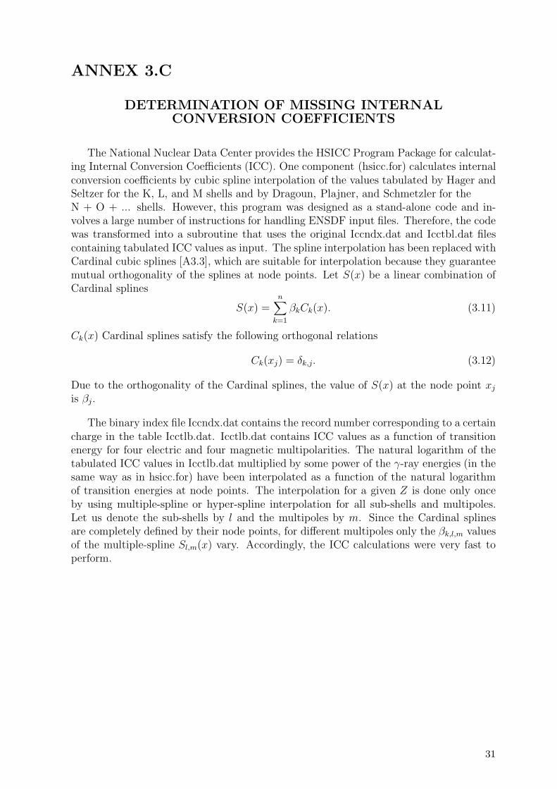
ANNEX 3.C

DETERMINATION OF MISSING INTERNALCONVERSION COEFFICIENTS

The National Nuclear Data Center provides the HSICC Program Package for calculat-ing Internal Conversion Coefficients (ICC). One component (hsicc.for) calculates internalconversion coefficients by cubic spline interpolation of the values tabulated by Hager andSeltzer for the K, L, and M shells and by Dragoun, Plajner, and Schmetzler for theN + O + ... shells. However, this program was designed as a stand-alone code and in-volves a large number of instructions for handling ENSDF input files. Therefore, the codewas transformed into a subroutine that uses the original Iccndx.dat and Icctbl.dat filescontaining tabulated ICC values as input. The spline interpolation has been replaced withCardinal cubic splines [A3.3], which are suitable for interpolation because they guaranteemutual orthogonality of the splines at node points. Let S(x) be a linear combination ofCardinal splines

S(x) =n∑

k=1

βkCk(x). (3.11)

Ck(x) Cardinal splines satisfy the following orthogonal relations

Ck(xj) = δk,j. (3.12)

Due to the orthogonality of the Cardinal splines, the value of S(x) at the node point xj

is βj.

The binary index file Iccndx.dat contains the record number corresponding to a certaincharge in the table Icctlb.dat. Icctlb.dat contains ICC values as a function of transitionenergy for four electric and four magnetic multipolarities. The natural logarithm of thetabulated ICC values in Icctlb.dat multiplied by some power of the γ-ray energies (in thesame way as in hsicc.for) have been interpolated as a function of the natural logarithmof transition energies at node points. The interpolation for a given Z is done only onceby using multiple-spline or hyper-spline interpolation for all sub-shells and multipoles.Let us denote the sub-shells by l and the multipoles by m. Since the Cardinal splinesare completely defined by their node points, for different multipoles only the βk,l,m valuesof the multiple-spline Sl,m(x) vary. Accordingly, the ICC calculations were very fast toperform.

31

ANNEX 3.D

CALCULATION OF DECAY PROBABILITIES

Calculations of total decay probabilities were based on the following rules: (i) if nodecay mode was given for a level, but there were de-exciting γ transitions, 100% electro-magnetic decay was assigned to the level (%IT=100%); (ii) if other decay modes beside theelectromagnetic were given, the percentage of electromagnetic decay mode was obtainedfrom the decay mode information. This procedure was identified by the notation %ITor %G in the decay record in the ENSDF files. First, the total relative electromagneticdecay probability was calculated

Ptot rel =Noγ∑k=1

Ik(1 + αk), (3.13)

where Ik is the relative γ intensity and αk is the ICC. The absolute electromagnetic decayprobability of the kth branch is

Pelectromagnetic,k =Ik(1 + αk)

Ptot rel· 0.01 ·%IT (%G), (3.14)

while the absolute γ-decay probability is

Pγ,k =Ik

Ptot rel· 0.01 ·%IT (%G). (3.15)

Other decay probabilities (particle) are given in the information on decay modes for alevel.

32

ANNEX 3.E

SIMPLE METHOD FOR DETERMINATION OFAPPROXIMATE NUCLEAR TEMPERATURE

A simple method of determining approximate nuclear temperature was developed andapplied to DLSL. Assuming that the constant temperature model describes level densitiesat low energies with some confidence, a useful expression was derived to determine thetemperature T . If one calculates the average level energy in continuous approximationwith the constant-temperature level density, the following expression is obtained:

Eaverage(Emax) =

1T

Emax∫−∞

Eexp(

E−U0T

)dE

exp(

Emax−U0

T

) = Emax − T, (3.16)

which is replaced by the following sum in discrete representation:

Eaverage(Emax) =

Nmax∑i=1

Ei

Nmax≈ Emax − T (3.17)

T can easily be obtained from Eq 3.17. This equation can be used to calculate thenuclear temperature by using the Emax obtained from the least-square fits (as comparedwith the T (A) function of Fig. 3.5). This new method is independent of the global fittingmethod because any functional dependence of the temperature on the mass number is notassumed, although the usage of Emax may introduce some correlation between the twomethods.

33

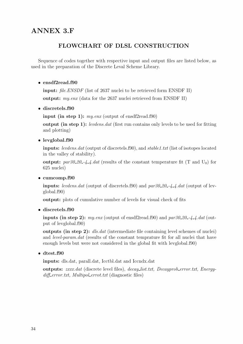
ANNEX 3.F

FLOWCHART OF DLSL CONSTRUCTION

Sequence of codes together with respective input and output files are listed below, asused in the preparation of the Discrete Leval Scheme Library.

• ensdf2read.f90

input: file.ENSDF (list of 2637 nuclei to be retrieved form ENSDF II)

output: my.enx (data for the 2637 nuclei retrieved from ENSDF II)

• discretels.f90

input (in step 1): my.enx (output of ensdf2read.f90)

output (in step 1): levdens.dat (first run contains only levels to be used for fittingand plotting)

• levglobal.f90

inputs: levdens.dat (output of discretels.f90), and stable1.txt (list of isotopes locatedin the valley of stability).

output: par30 20 -4 4.dat (results of the constant temperature fit (T and U0) for625 nuclei)

• cumcomp.f90

inputs: levdens.dat (output of discretels.f90) and par30 20 -4 4.dat (output of lev-global.f90)

output: plots of cumulative number of levels for visual check of fits

• discretels.f90

inputs (in step 2): my.enx (output of ensdf2read.f90) and par30 20 -4 4.dat (out-put of levglobal.f90)

outputs (in step 2): dls.dat (intermediate file containing level schemes of nuclei)and level-param.dat (results of the constant temprature fit for all nuclei that haveenough levels but were not considered in the global fit with levglobal.f90)

• dtest.f90

inputs: dls.dat, parall.dat, Icctbl.dat and Iccndx.dat

outputs: zxxx.dat (discrete level files), decay list.txt, Decayprob error.txt, Energy-diff error.txt, Multipol errot.txt (diagnostic files)

34

REFERENCES TO ANNEXES

[A3.1] BELGYA, T., MOLNAR, G., FAZEKAS, B., OSTOR, J., Histogram plots andcutoff energies for nuclear discrete levels, INDC(NDS)-367, IAEA, Vienna (1997).

[A3.2] INTERNATIONAL ATOMIC ENERGY AGENCY, Handbook for Calculationsof Nuclear Reaction Data - Reference Input Parameter Library,IAEA-TECDOC-1034 (1998).

[A3.3] WINTERBON, K.B., Nucl. Phys. A246 (1975) 293.

[A3.4] ERICSON, T., Adv. Phys. 9 (1960) 425.

[A3.5] GILBERT, A., CAMERON, A.G.W., Can J. Phys. 43 (1965) 1446.

35

4 AVERAGE NEUTRON RESONANCE

PARAMETERS

Coordinator: A. Ignatyuk

Summary

Average resonance parameters included in the recommended RIPL-1 file were tested andrevised during RIPL-2. The differences between the recommended and alternative fileswere analyzed on the basis of the last compilation of the resolved resonance parameters.Recommended data were corrected for some nuclei, and the number of nuclei has beenextended to 297. Along with the data for the s-wave neutron resonances, the evaluationsof the average parameters for the p-wave resonances have been added to the RIPL-2library. The file formats are explained in the corresponding readme file.

Parameters required for statistical model calculations are neutron strength functions,average radiative widths and the average spacing of resonances. These parameters aregenerally obtained from the analysis of parameter sets for the resolved resonances. Experi-mental resolution and sensitivity limits create incomplete (missing resonances) or distorted(errors in width determination) information on the resonance parameters. Therefore, theaverage widths and resonance spacings cannot be directly deduced from available res-onance sequences, and should always be estimated while taking into account missingresonances. Various methods for statistical analysis of missing resonances have been de-veloped, and most of them were applied to evaluate average resonance parameters duringthe RIPL project. Advantages and shortcomings of such methods are briefly discussedbelow in order to obtain some objective estimation of the accuracy of the recommendedparameters. Before describing the statistical methods for resonance analysis, one shouldbe aware that statistical methods of resonance analysis work only when applied to pureresonance samples - results become less and less accurate with sample deficiencies.

Sample cases of pure resonances are rare. Such difficulties are overcome by adoptingdifferent statistical analysis methods as well as sampling criteria to identify a reducedsample in which missing resonances and/or distortions are reduced. Thus, determinigaverage resonance parameters is an iterative procedure in which one tries to reach con-vergence of results from different methods of analysis. The spread of values from differentstatistical procedures indicates that the uncertainties are affecting the results. However,in many cases such an iterative procedure is not sufficient to guarantee the correctnessof the parameters. Whenever possible, they should be validated by use of supplementaryinformation such as capture cross sections and radiative widths.

37

4.1 Evaluation methods

The neutron strength functions for a given orbital angular momentum l are defined bythe relationship

Sl =< gΓl

n >

(2l + 1)Dl=

1

(2l + 1)∆E

∑r

grΓlnr , (4.1)

where the summation is performed over N resonances in the energy interval ∆E;gr = (2Jr + 1)/2(2I0 + 1) is the statistical weight factor that depends on the angularmomentum Jr of a resonance and the spin I0 of the target nucleus; Γl

nr are the reducedneutron widths of resonances, and Dl is the average resonance spacing defined as

Dl = ∆E/(N − 1). (4.2)

The reliable identification of s- and p-wave resonances is most important for an accurateevaluation of the average parameters. If such an identification can be made, the neutronstrength functions can be simply evaluated from the linear approximation of the cumula-tive sum of the products grΓ

lnr . Departure from linearity may indicate missing resonances.

The relative error of the evaluation can be defined from the equation

δSl

Sl=√

2/N, (4.3)

which is based on an asymptotic estimate for the variance of the sum of neutron widthsdistributed in accordance with the Porter-Thomas law [4.1].

Dominant contributions to the sum in Eq. (4.1) for s-neutrons are given by resonanceswith large neutron widths; missing weak resonances or admixture of p-wave resonanceshave a rather small effect on the evaluation of the strength functions. The situation is notso favorable for p-neutrons, for which the strength function can be strongly distorted byany admixture of incorrectly identified s-wave resonances. This is the main reason thatthe relative accuracies of p-wave strength functions for many nuclei are much lower thanfor the s-waves.

For a rather full set of resonances the relative statistical error of the resonance spacingcan be determined by the relationship

δDl

Dl=

0.45√

lnN + 2.18

N≈ 1

N, (4.4)

which was obtained by Dayson and Mehta for the Gaussian orthogonal ensemble [4.2].Obviously, missing resonances in the analyzed set result in an error that essentially exceedsthe statistical error. Thus, an estimation of the missing resonances is crucial for anaccurate evaluation of the average resonance spacings.

Three approaches were developed to account statistically for the missing or erroneouslyidentified resonances: (i) methods that exploit the statistics of level spacings, (ii) methodsbased on the fit of the reduced neutron width distribution by the Porter-Thomas law,(iii) methods that use combined simulation of the level and width statistics. Both theadvantages and weaknesses of these various methods have been broadly discussed in Refs.[4.3–4.8]. Some new developments related to the third type of method were proposedrecently [4.9–4.12].

38

The simplest method of resonance analysis is the staircase plot of the cumulativenumber N(E) of resonances as a function of energy. It is usually assumed that at lowenergies there are no missing resonances, and a linear approximation of this part of theplot gives a direct estimation of Dl. A variation of this method is the approach basedon ∆3 statistics given by Dayson and Mehta [4.2]. The best fit of N(E) is determinedthrough a least-squares study of the parameter

∆ = min

[1

∆E

∫ ∆E

0[N(E)−AE − B]2dE

]. (4.5)

For a complete set of levels, the value and the variance of this parameter are defined bythe relationships:

∆3 =< ∆ >=1

π2(lnN − 0.0687), σ =

1

π2

√4π2

45+

7

24= 0.11. (4.6)

Obviously, absence of levels or presence of spurious levels from another sequences increases∆3. Therefore, if the fitted value of ∆ satisfies the condition ∆3 − σ < ∆ < ∆3 + σ, theanalyzed set of resonances may be considered as a pure and complete set. Unfortunately,∆3 statistics provide no means of correcting an inadequate set of resonance parameters.Besides, one finds in practice that the ∆3 test criteria are often satisfied for samples thatare known to be neither pure nor complete [4.6, 4.8].

In contrast to the spacing distribution, the neutron width distribution is only slightlyaffected by missing or spurious weak resonances. The upper part of the Porter-Thomasdistribution, corresponding to strong resonances, can be regarded as virtually unper-turbed. A number of resonances that have the reduced neutron width above a given valueare described by the function

N(Γ) = N0

∫ ∞

Γ/Γ

exp(−x/2)dx√2πx

= N0

[1− erf

√Γ/2Γ

]. (4.7)

Thus, by fitting the corresponding distribution of neutron widths with a maximum like-lihood approach, we can find both the average reduced neutron width and total numberof resonances N0 at the considered energy interval. Various versions of this method weredeveloped to take into account energy variations of the measurement threshold and otherexperimental conditions [4.8, 4.9].

The third class of methods attempts to account simultaneously for limitations imposedon estimations of a mean width and resonance spacing by the Wigner and Porter-Thomaslaws. Simulations of the neutron cross section by the Monte-Carlo methods that includeexperimental resolution and other conditions are applied in most cases. Some analyticaltreatments that could replace the Monte-Carlo simulation for some calculations werediscussed in Ref. [4.9].

The conclusion that can be formulated on the basis of the resonance parameter analy-ses performed by different groups is that none of the methods guarantees an unambiguousidentification of missed or spurious resonances. Critical analyses of the experimental con-ditions and approaches used to obtain individual resonance parameters are very importantin many cases. Priority in average parameter evaluations should be given to the qualityof the selected resonance set rather than to the total number of resonances considered

39

[4.9, 4.13]. Only for a rather small number of nuclei is the accuracy of the evaluated res-onance spacings better than 10%. The best examples of such nuclei are U-235 and U-238for which the relative errors of the recommended D0 are better than 2%, and Pu-239,Pu-240 and Pu-242 for which such errors are about 5% [4.9, 4.11].

4.2 Files of average neutron resonance parameters

Complete tables of average resonance parameters provided by Beijing, Bologna and Ob-ninsk groups were collected during the course of the RIPL-1 project. All these parametersare mainly based on the analysis of the resolved resonance parameters presented in thewell-known BNL compilation [4.14, 4.15]. Despite the common base, many discrepancieswere found between the average parameter estimations. These discrepancies were ratherlarge when compared to the parameter uncertainties, especially for cases with less than20 resonances.

After consideration of the existing discrepancies, the Beijing and Obninsk groups re-analyzed some of their previous evaluations, and prepared updated versions of the averageresonance parameters. Agreement between the updated parameters has been significantlyimproved for most of the nuclei, although the uncertainties quoted for the Obninsk eval-uations were systematically higher than the uncertainties given in the original BNL eval-uations [4.14, 4.15] and the revised Beijing data. This difference was shown to be mainlyconcerned with the reduction of the energy interval that the Obninsk group used to im-prove the quality of the analyzed sets of resonances in accord with the statistical methodsdescribed above. Taking into account substantial differences between the uncertaintiesobtained by the various methods, those of the Obninsk group seem more reliable thanothers. Accordingly, the Obninsk evaluation of the average resonance parameters wasincluded in RIPL-1 as the recommended file, and the Beijing evaluation as the alterna-tive [4.16]. The Minsk evaluation of the average resonance parameters for the actinideswas also included as an alternative file, and the additional compilations of the averageresonance spacings (mengoni gc.dat and iljinov gc.dat files) were included in Segment 5of the RIPL-1 Starter File [4.16], because of their relevance to nuclear level densities.

The recommended data sets have been extended under the RIPL-2 project to includethe average parameters for p-wave neutron resonances along with the s-wave resonance pa-rameters considered previously. Although the accuracy of the data for p-wave resonancesis certainly not as good as for s-wave resonances, such improved data are important inthe optical and statistical models. Another task of the RIPL-2 project was to test andrevise the previously recommended parameters.

A reliable separation of p-wave resonances from the background of stronger s-waveresonances plays a crucial role in estimating the average resonance parameters. Thus,trustworthy results for the p-wave resonance parameters can only be obtained under thesimultaneous analysis of the resolved resonance data for both s- and p-wave neutrons.Such an analysis for nuclei included in the RIPL-1 list of recommended parameters wasperformed by the Obninsk group [4.17], and the corresponding resonance spacings D1,the neutron strength functions S1, and the average radiative widths of p-wave resonanceswere added to the RIPL-2 database.

40

Another problem is to produce a complete list of recommended parameters. In theoriginal BNL compilation [4.14, 4.15], the average resonance parameters were obtained forabout 230 nuclei; Iljinov et al. [4.18] compiled the resonance spacings for 284 nuclei; theBeijing compilation reports data for 344 nuclei [4.19]; however, the recommended RIPL-1file is limited to only 281 nuclei. A careful review of the Beijing compilation shows that 35out of 344 nuclei contain no data quantifying the neutron strength functions and a numberof resonances are set to zero. This observation indicates that the resonance spacings forthese nuclei were not obtained from the analysis of experimental data, but rather from thesystematics of neighboring nuclei. Such systematics could be useful for many applications,but the results should not be mixed with the direct experimental data, and therefore havebeen removed from the RIPL-2 database. All issues related to the resonance spacingsystematics that are connected with nuclear level densities are considered in Chapter 6.

Some skepticism can arise with respect to the recommended parameters of nuclei forwhich data are available for a rather small number of resonances, particularly for about45 nuclei in RIPL-1 in which the number of resonances are equal or less than five. Anystatistical analysis of such data is doubtful. Nevertheless, we decided to include such casesin the recommended file to provide an estimate that is certainly better than nothing. So allnuclei available in the alternative files of RIPL-1 but not in the recommended file were re-analyzed on the basis of the last compilation of the resolved resonance parameters [4.20].As a result, 16 nuclei were added to the list of average resonance parameters included inthe RIPL-2 file. This file was tested by the Brussels group in their microscopic calculationsof nuclear level densities, and some misprints were corrected in the final version of theRIPL-2 file.

Independent analyses of the resonance parameters for about 20 nuclei have been per-formed by the BNL group [4.21]. They re-evaluated the resonance spacings, the neutronstrength functions and the radiative widths for the most important fission products. Inmost cases, the new BNL results overlap with the RIPL-1 recommended parameters withinthe bounds of the accepted uncertainties.

The s-wave resonance spacings included in RIPL-2 are shown in Fig. 4.1, along withthe Beijing evaluation [4.16] and BNL data. Uncertainties for most of the data do notexceed the sizes of the symbols, showing that the results of all the evaluations agree ratherwell for nuclei with more than 30 known resonances. For other nuclei, the data included inthe RIPL-2 file seem preferable for two reasons: (i) more accurate selection of the energyinterval used for the average parameter evaluations and (ii) more reliable estimations ofthe quoted uncertainties.

The resonance spacings of the p-wave resonances are shown in Fig. 4.2. These datawere obtained for a substantially smaller number of nuclei than for the s-wave resonances.Nevertheless, the p-resonance spacing data are very important in testing the consistencyof the results. Based on the general statistical properties of nuclear levels, the spacingsof the s- and p-wave resonances should be related (D1 = D0/3) at least for nuclei farfrom the magic numbers. This relationship is also useful for a coarse estimation of thes-resonance spacing when only p-resonance data are available. Data included in RIPL-2for the s-wave neutron strength functions are shown in Fig. 4.3, and compared withBNL data [4.14, 4.15] corrected in a new evaluation [4.21]. For most cases, there are nosignificant differences between the two evaluations. As explained above, the

41

0 50 100 150 200 25010-4

10-3

10-2

10-1

100

101

102

103

Beijing BNL RIPL-2

Mass number

Do

, keV

Figure 4.1: Average resonance spacings for the s-wave neutron resonances included in theBNL [4.14, 4.15, 4.21], Beijing [4.16, 4.19] and RIPL-2 evaluations.

0 50 100 150 200 25010-3

10-2

10-1

100

101

102

BNL Obninsk

Mass number

D1

, keV

Figure 4.2: Average resonance spacings for the p-wave neutron resonances included in theBNL [4.14, 4.15] and RIPL-2 evaluations.

42

0 50 100 150 200 250

0,1

1

10

BNL RIPL-2

Mass number

S0 1

0 4

Figure 4.3: The s-wave neutron strength functions included in the BNL [4.14, 4.15, 4.21]and RIPL-2 evaluations. Uncertainties are shown for the RIPL-2 evaluations only.

uncertainties quoted in the RIPL-2 file are slightly higher than those in the BNL evalu-ation, partially because they take into account sample quality in addition to statisticalerrors.

Similar results for the p-wave neutron strength functions are presented in Fig. 4.4.The BNL compilation includes some additional data on the p-wave strength functions thatwere obtained from neutron cross-section analyses in the unresolved resonance region.However, such analyses require some additional, model-dependent approximations, andtherefore we decided to limit the RIPL-2 resonance files to the data based on the resolvedresonance parameters observed directly.

Average radiative widths included in the RIPL-2 files are shown in Figs. 4.5 and 4.6for the s- and p-wave resonances, respectively. The recommended values obtained bydifferent groups agree with each other in general [4.16]. However, we note that for manynuclei the average widths are given without any uncertainties in the BNL and Beijingevaluations. Under such circumstances, the uncertainties provided in the RIPL-2 fileshould be adopted.

43

0 50 100 150 200 25010-1

100

101

BNL Obninsk

Mass number

S1 1

04

Figure 4.4: The p-wave neutron strength functions included in the BNL [4.14, 4.15] andRIPL-2 evaluations.

0 50 100 150 200 25010

100

1000

BNL RIPL-2

Mass number

Gg, m

eV

Figure 4.5: Average radiative widths for the s-wave neutron resonances included in theBNL and RIPL-2 evaluations.

44

0 50 100 150 200 250101

102

103

BNL Obninsk

Mass number

Gg (

meV

)

Figure 4.6: Average radiative widths for the p-wave neutron resonances included in theBNL [4.14, 4.15] and RIPL-2 evaluations.

4.3 Conclusions and recommendations

All recent evaluations by the Beijing, Minsk, Obninsk, and Troitsk groups have beenincluded in the RIPL-1 database, and the recommended RIPL-1 data were tested andrevised during the RIPL-2 project. Previous data were corrected and extended by takinginto account recent experimental data. In addition to the data for the s-wave neutronresonances, new evaluations of the average parameters for the p-wave resonances havebeen included in the RIPL-2 library.

REFERENCES

[4.1] PORTER, C.E., THOMAS, R.G., Phys. Rev. 104 (1956) 483.

[4.2] PORTER, C.E. (Ed.), Statistical Theories of Spectra, Academic Press, New York(1965).

[4.3] MEHTA, M.L., Random Matrices, Academic Press, New York (1967).

[4.4] LYNN, J.E., Theory of Neutron Resonance Reactions, Clarendon Press, Oxford(1968).

[4.5] CAMARDA, H.S., et al., in Statistical Properties of Nuclei, CARD., J.B., (Ed.),Plenum Press, New York (1972) 285.

45

[4.6] LIOU, H.I., CAMARDA, H.S., WYNCHANK, S., SLAGOWITZ, M., HACKEN,G., RAHN, F., RAINWATER, J., Phys. Rev. C5 (1972) 974.

[4.7] DELFINI, G., GRUPPELLAAR, H., in Proc. Meeting on Neutron Cross Sectionsof Fission Product Nuclei, COCEVA, C., PANINI, G.C., (Eds.), NEANDC(E)-209,Bologna (1979) 169.

[4.8] FORT, E., DERRIEN, H., LAFOND, O. in Proc. Meeting on Neutron CrossSections of Fission Product Nuclei, COCEVA, C., PANINI, G.C., (Eds.), NE-ANDC(E) 209, Bologna (1979) 121.

[4.9] FROHNER, F.H., in IAEA Advisory Group Meeting on Basic and Applied Prob-lems of Nuclear Level Densities, BHAT, M.R., (Ed.), BNL-NCS-51694, Brookhaven(1983) 219.

[4.10] RIBON, P., ibid., 245.

[4.11] ZONGDI SU, et al., in Proc. Meeting on Nuclear Data Evaluation Methods, DUN-FORD, C., (Ed.), New York (1992).

[4.12] PORODZINSKI, Yu.V., SUKHOVITSKI, E.Sh., in Proc. ISTC Workshop on Nu-clear Data for Minor Actinides, JAERI-97-001, Tokai (May 1996) 34.

[4.13] BELANOVA, T.S., IGNATYUK, A.V., PASHCHENKO, A.B., PLYASKIN, V.I.,Radiative Neutron Capture - Handbook (in Russian), Energoatomizdat, Moscow(1986).

[4.14] MUGHABGHAB, S.F., DIVADEENAM, M., HOLDEN, N.E., Neutron Cross Sec-tions, Vol. 1, part A, Academic Press, New York and London (1981).

[4.15] MUGHABGHAB, S.F., Neutron Cross Sections, Vol. 1, part B, Academic Press,New York and London (1985).

[4.16] INTERNATIONAL ATOMIC ENERGY AGENCY, Handbook for Calculationsof Nuclear Reaction Data - Reference Input Parameter Library, IAEA-TECDOC-1034, Vienna (1998).

[4.17] IGNATYUK, A.V., Low Energy Neutron Physics, Landolt-Boernstein Series 16A,part 2, Springer, Berlin (2000) 1.

[4.18] ILJINOV, A.S., MEBEL, M.V., BIANCHI, N., DE SANCTIS, E., GUARALDO,C., LUCHERINI, V., MUCCIFORA, V., POLLI, E., REOLON, A.R., ROSSI, P.,Nucl. Phys. A543 (1992) 517.

[4.19] ZONGDI SU, et al., Contribution to Third CRP Meeting on RIPL, Trieste, May1997.

[4.20] SUKHORUCHKIN, S.M., et al., Low Energy Neutron Physics, Landolt-BoernsteinSeries 16B, Springer, Berlin (2000).

[4.21] OH, SOO-YOUL, CHANG, J., MUGHABGHAB, S.F., Neutron Cross SectionEvaluations of Fission Products Below the Fast Energy Region, BNL-NCS-67469(ENDF-362) (2000).

46

5 OPTICAL MODEL PARAMETERS

Coordinators: O. Bersillon and P.G. Young

Summary

The optical model segment of the Reference Input Parameter Library is described. Avail-able files include a library of phenomenological optical model potentials (OMP) for inci-dent neutrons, protons, deuterons, tritons, 3He and 4He particles; a microscopic opticalmodel code for incident nucleons; several retrieval and utility codes for accessing the OMPlibrary; definition of the format of the OMP library; and user information for the variouscodes. Global as well as nuclide-specific potentials are included that utilize spherical,vibrational, dispersive and rotational models. The optical model parameterizations in thelibrary are given in a general format that allows for easy expansion. Recommendations forthe use of the library are given, together with user instructions for the various computercodes.

The optical model provides the basis for many theoretical analyzes and/or evaluationsof nuclear cross sections that are used in providing nuclear data for applied purposes. Aswell as offering a convenient means for the calculation of reaction, shape elastic and (neu-tron) total cross sections, optical model potentials are widely used in quantum-mechanicalpre-equilibrium and direct-reaction theory calculations, and (most importantly) in sup-plying particle transmission coefficients for Hauser-Feshbach statistical-theory as used innuclear data evaluations.

The importance of optical model parameterizations is made even more apparent bythe worldwide diminution of experimental facilities for low-energy nuclear physics mea-surements and the consequent increased reliance on theoretical methods for providingnuclear data for applications. Therefore, the preservation of past work aimed at describ-ing experimental results with optical model potentials is vital for the future developmentof nuclear databases. Additionally, the availability and use of microscopic optical modelcodes is important for predicting data for target nuclei far from the line of stability, wherephenomenological models might not be valid.

The optical model segment of RIPL-2 is aimed at extending the library of opticalmodel parameterizations developed under the RIPL-1 project [5.1], and providing accessto a microscopic optical model code. The product of this activity for phenomenologicaloptical potentials is an optical model potential (OMP) library that contains reliable, state-of-the-art parameterizations for the conventional optical model codes used in calculationsof nuclear data for applications. In addition to preserving optical model parameterizationsfor future activities, the library offers a convenient means for evaluators to access a wide

47

body of information on the optical model. Subroutines have been developed for readingand writing the data library and for creating convenient summaries of the library. Pro-cessing codes are provided that permit direct interfacing of the library with the selectedoptical model codes.

The OMP library is organized in two parts: an archival file and a user file. Thearchival file contains all potentials compiled so far, totaling some 533 entries; the user fileis a subset of the archival file and contains 406 potentials. The focus of the RIPL-2 studieswas the user library, which contains the most useful optical potentials for calculating datafor applications. The format of the archival library is identical to the user library, and thevarious retrieval and utility codes that are provided work equally well with either library.Details of the phenomenological library and supporting codes are given below.

In addition to the OMP library, a semi-microscopic optical model code is also suppliedand described in Section 5.2. This model should mainly be used when experimental dataare missing.

5.1 Phenomenological parameterizations

5.1.1 Description of the potential

One of the primary goals of the optical model segment is to provide a format for opticalmodel parameterizations that is general enough to cover all commonly used phenomeno-logical potential representations and that is easily expanded for additional types of opticalpotentials. We have focused on standard Schrodinger-type forms of optical model poten-tials, and have included spherical, coupled-channel rotational, vibrational and dispersiveoptical models.

As presently formulated, potentials of the form

V (r) = −VR fR(r) − iWV fV (r) + 4aV D VDd

drfV D(r) + 4iaWD WD

d

drfWD(r) +

λ2π

r[VSO

d

drfV SO(r) + iWSO

d

drfWSO(r)] σ · l (5.1)

are allowed, in which VR and WV are the real and imaginary volume potential well depths,VD and WD are the real and imaginary well depths for the surface derivative term, VSO

and WSO are the real and imaginary well depths for the spin-orbit potential, and λ2π is

the pion Compton wavelength squared (� 2 fm2). The quantity σ · l is the scalar productof the intrinsic and orbital angular momentum operators and is given by

σ · l = l for j = l +1

2

= −(l + 1) for j = l − 1

2(5.2)

where fi(r) are radial-dependent form factors and are defined below (Section 5.1.5).

Any incident particle is permitted by the format, but we have limited our initiallibrary to incident neutrons, protons, deuterons, tritons, 3He and 4He particles. Our

48

approach is to supply a general form for optical model potentials that is an extension of therepresentation implemented in the SCAT2000 optical model code [5.2] and that describesmost of the parameterizations that have been commonly used in the past. Additionally,three specialized formats are formulated that describe particular less common forms ofpotentials, but which offer promise as being important for applied purposes.

Many high energy potentials are obtained with the use of the relativistic kinematics(see Annex 5.D). It should be noted here that the relativistic OMPs given in the libraryinclude the γ relativistic factor [5.3].

5.1.2 Dispersive relations

The dispersive optical model is a natural result of the causality principle: a scattered wavecannot be emitted before the arrival of the incident wave. This introduces an integralrelationship [5.4] which links the real and imaginary parts of the nuclear potential

∆V (E) =1

πP∫ ∞

−∞W (E ′)E ′ − E

dE′ .

where W is either the volume or the surface absorption potential. This addition provides amore realistic description of the energy dependence of the optical potential and enables theprediction of single-particle, bound-state quantities (such as binding energies, occupationprobabilities and spectroscopic factors). There are few analyses that include dispersiverelationships. One reason is that the integrals are analytical for only a very restrictednumber of absorption potential energy dependences (piecewise linear [5.2] or Brown andRho form [5.5, 5.6]). Precise numerical calculation of these integrals might make the useof the dispersion approach easier [5.7].

An example is given in Ref. [5.8] of the extension of the dispersive optical modelapproach to permanently deformed nuclei.

5.1.3 Nucleon-nucleus potentials

Individual Nucleus Potentials

The bulk of the nucleon-nucleus potentials in the OMP library is for single target nuclei(or perhaps for a very narrow range of neighboring targets) and cover a range of incidentenergies. These potentials are usually the most accurate for specific targets and should beconsidered whenever accuracy is imperative. There is one important series of potentialsthat, while given for specific targets, were derived as part of a comprehensive analysiscovering targets from 24Mg to 209Bi. These are the spherical optical model potentialsby Koning and Delaroche [5.9]. Other significant individual nuclide potentials are thoseby Arthur [5.10] and the extensive lists of potentials used in China [5.11] and Japan[5.12] for fission products. All of the rotational model potentials described below are inthe form of individual nucleus potentials with relatively small ranges of validity in Z andA.

49

Global potentials

The use of the term “global” refers to optical model potentials that cover a wide rangeof incident energy and target nuclei. The most important potentials that are global forboth incident neutrons and protons are those of

• Koning and Delaroche [5.9] (Z=12-83, A=27-209, E=0.001-200 MeV), and

• Madland [5.3] (Z=6-82, A=12-208, E=50-400 MeV).

In addition to incorporating improved methodology, these potentials are the most recentlydeveloped global potentials and, as such, their analyses have drawn upon a wider rangeof experimental data than the older potentials.

Other older global potentials that cover both incident neutrons and protons are thoseof

• Becchetti and Greenlees [5.13] (Z=20-92, A=40-238, E=10-50 MeV),

• Walter and Guss [5.14] (Z=26-82, A=54-208, E=10-80 MeV), and

• Varner et al. [5.15] (Z=20-83, A=40-209, E=16-65 MeV).

Older global potentials developed exclusively for incident neutrons are those of

• Moldauer [5.16] (Z=20-83, A=40-209, E=0.001-5 MeV),

• Wilmore and Hodgson [5.17] (Z=20-92, A=40-238, E=0.01-25 MeV),

• Engelbrecht and Fiedeldey [5.18] (Z=20-83, A=40-210, E=0.001-155 MeV),

• Strohmaier et al. [5.19] (Z=23-41, A=50-95, E=0.001-30 MeV).

For incident protons alone, there are the potentials of

• Menet et al. [5.20] (Z=6-82, A=12-208, E=30-60 MeV),

• Perey [5.21] (Z=16-49, A=30-100, E=0.01-22 MeV), and

• Patterson et al. [5.22] (Z=20-82, A=48-208, E=25-45 MeV).

Coupled-channels potentials

The RIPL-2 OMP library contains 33 neutron and 8 proton coupled-channels poten-tials for ground-state rotational bands. These potentials have been necessarily developedfor more limited target Z and A ranges, as they are dependent upon the structure ofeach target nucleus. For incident neutrons, the targets include 151−153Eu, 165Ho, 169Tm,

50

182−186W, 185,187Re, 197Au and a number of actinides between 232Th and 252Cf. In eachcase, the structure information is provided in the OMP library for the target nuclei forwhich the potential was determined. It is possible for the user to use these potentials overa broader range of target nuclei, most probably with reduced accuracy, although the usermust provide the required structure information.

Coupled-channels potentials for incident protons are provided for the same targetnuclei, except that only one potential is included for actinides. These potentials weredetermined with the neutron potentials using the Lane model [5.23].

5.1.4 Complex-particle potentials

A limited number of spherical potentials are included for complex particles.

For incident deuterons, there are global potentials from

• Bojowald et al. [5.24] (Z=6-82, A=12-208, E=20-100 MeV),

• Lohr and Haeberli [5.25] ( Z=20-83, A=40-209, E=8-13 MeV), and

• Perey and Perey [5.26] (Z=20-82, A=40-208, E=11-27 MeV).

Additionally, there are individual target potentials for 5 nuclei between 40Ca and 208Pbby Daehnick et al. [5.27], each covering the incident deuteron energy range from 11.8 to90 MeV.

For incident tritons and 3He particles, the global potentials of Becchetti and Greenlees[5.28] (Z=20-82, A=40-208, E=1-40 MeV) are included. The energy dependence of thetriton potential is based on the 3He potential, which covers the same energy range for thesame target charge and mass range.

In the case of incident alpha particles, the OMP library includes global potentials from

• McFadden and Satchler [5.29] (Z=8-82, A=16-208, E=1-25 MeV),

• Avrigeanu et al. [5.30] (Z=8-96, A=16-250, E=1-73 MeV),

• Huizenga and Igo [5.31] (Z=10-92, A=20-235, E=1-46 MeV), and

• Strohmaier et al. [5.19] (Z=20-45, A=40-100, E=1-30 MeV).

Also included in the RIPL-2 optical file space is a code that can be used to obtain phe-nomenological alpha-particle potentials (om-alpha.f). This code was developed by Kumarand Kailas [5.32] for the RIPL-2 co-ordinated research project, and utilizes systematics ofthe nuclear radius and slope as well as real potential microscopic volume integrals fromearlier analyzes of alpha optical model potentials. The new global potential is valid forincident alpha energies near the Coulomb barrier up to 150 MeV and for target nuclei overthe mass range A = 16 to 208. The elastic and reaction cross sections calculated with this

51

model show satisfactory agreement with experimental data for the limited cases checkedso far. At energies below the Coulomb barrier, the potential has not been thoroughlytested.

5.1.5 Format of OMP library

A complete description of the format of the OMP library is given in Annex 5.A, so onlya summary is given here. The format allows parameterizations for spherical, coupled-channels rotational, vibrational and non-axial deformed optical models. Potentials may berelativistic or non-relativistic, dispersive or non-dispersive. The format allows for inclusionof structure data for coupled-channels rotational, vibrational and non-axial deformedmodels.

The general form of the optical model potential is the following:

Vi(E) = α1 + α7η + α8∆c + α9A + α10A1/3 + α11A

−2/3 + α12∆c′ +

(α2 + α13η + α14A)E + α3E2 + α4E

3 + α6

√E +

(α5 + α15η + α16E) ln(E) + α17∆cE−2 (5.3)

where Vi(E) designates the ith term of the potential (for example, VR, WD, VSO, etc.)at incident laboratory energy E, η = (N − Z)/A, N and Z are the neutron and protonnumbers of the target nucleus, and A is the integer atomic mass of the target, i.e., A= N + Z. Two different forms of correction terms for Coulomb repulsion with incidentprotons are provided:

∆c =0.4 Z

A1/3and ∆c′ =

1.73 Z

Rc(5.4)

where Rc is the Coulomb radius. The coefficients that multiply ∆c and ∆c′ are usuallyzero for incident neutrons.

Each of the potential terms in Eq. 5.1 can be represented over any number of definedenergy ranges using as many of the terms given in Eq. 5.3 as required, with the coefficientsof the unused terms set to zero.

Either Woods-Saxon or Gaussian form factors are permitted for the fi(r) terms inEq. 5.1:

fi(r) =[1 + exp

(r − Ri

ai

)]−1

(Woods-Saxon form) (5.5)

or

fi(r) = exp

[−(r − Ri)

2

a2i

](Gaussian form). (5.6)

The nuclear radius is given by Ri = ri A1/3, where ri is given by

ri(E) = β1 + β2E + β3η + β4A−1 + β5A

−1/2 + β6A2/3 + β7A + β8A

2 +

β9A3 + β10A

1/3 + β11A−1/3, (5.7)

52

and a similar form is used for the diffuseness (ai):

ai(E) = δ1 + δ2E + δ3η + δ4A−1 + δ5A

−1/2 + δ6A2/3 + δ7A + δ8A

2 +

δ9A3 + δ10A

1/3 + δ11A−1/3. (5.8)

βi and δi are constants that are given in the OMP library. Note that the β11A−1/3

term in Eq. 5.7 permits the inclusion of a constant (A-independent) quantity to the radiusthat is Ri = ro + r′i A

1/3 = β11 + r′i A1/3.

In addition to the general formula given in Eq. 5.7, three specialized formats areprovided for inclusion of potentials by Smith et al. [5.33], Engelbrecht and Fiedeldey[5.18], Varner et al. [5.15], and Koning and Delaroche [5.9]. The first two special formsare described in the RIPL-1 report [5.1]; whereas the third is used with potentials fromKoning and Delaroche, has changed since RIPL-1, and is summarized below.

The format used for the Koning and Delaroche potentials, as well as that of Koningel al. [5.34], is given by the following expression:

Vi = b1[1− b2(E − Ef ) + b3(E −Ef )2− b4(E − Ef)3] + b5 +

b6(E − Ef )n/[(E − Ef )n + bn7 ] + b11 exp[−b12(E − Ef )] +

b8 exp[−b9(E −Ef )](E − Ef)n/[(E − Ef)

n + bn10] (5.9)

where Ef is the Fermi energy and is provided in the library. Likewise, the various bi aredetermined from parameters in the library. The format and relationships are fully definedin Annex 5.A.

5.1.6 Contents of OMP library

The OMP library is given in two parts: an archival file and a user file. The archival filecontains all potentials compiled so far and totaling 533, of which 287 are potentials forincident neutrons, 146 potentials for protons, 11 for deuterons, 26 for tritons, 53 for 3Heparticles, and 10 for incident alpha particles. The user file is a subset of the archival filewith all single-energy potentials eliminated, and contains 406 entries.

Each potential included in RIPL is given a unique reference number, according toa system that is described in Annex 5.B. This numbering system was adopted in orderto separate the potentials for different incident particles into different reference numberregions, and to provide approximate information on the sources of the various potentials bygeographical region. For example, the latter information might be used if only potentialsfrom a particular source are adopted for a given set of calculations.

An example of a complete entry for one reference in the library is given in Annex 5.C,following the format given in Annex 5.A. The reference number (5003) indicates that theincident particle is a proton, and that the source of the potential is a laboratory in theUnited States of America.

Summary information on all the potentials compiled to date is given in Annex 5.D,together with references for each potential. The user library to date includes:

53

• 283 optical model parameterizations for incident neutrons,

• 101 parameterizations for incident protons,

• 8 parameterizations for incident deuterons,

• 1 parameterization for incident tritons,

• 3 parameterizations for 3He particles, and

• 10 parameterizations for incident alpha particles.

5.2 Microscopic optical model

The phenomenological parameterizations described in the previous section are suitable ifthere are sufficient experimental data to constrain the optical model parameters. If thesedata are too sparse or totally lacking, one has to move to global parameterizations or, ina more physical way, to a semi-microscopic approach as described in Ref. [5.35].

The potentials in this model are calculated by folding the target radial matter densitywith an optical potential in nuclear matter based on the Bruckner-Hartree-Fock work ofJeukenne et al. [5.36]. Parameterization of this potential in nuclear matter was revisedby unifying the low and high energy components [5.35, 5.37], and thus making the semi-microscopic model applicable in the nucleon energy range from 1 keV to 200 MeV andfor spherical nuclei with mass number A > 30.

The semi-Microscopic Optical Model is implemented in the MOM package which isincluded in the optical directory.

5.3 Validation

Validation of the potentials in the library has been carried out at several levels. In additionto considerable proof reading, several of the potentials contained in the RIPL-2 libraryhave been tested by Kumar et al. [5.38] against experimental data. In every case wherelocal potentials were compared to global potentials, the local parameterizations producedbetter agreement with the experimental data than did the global potentials. Additionally,volume integrals from several well-known global potentials were compared to “best-fit”potentials for the 208Pb + n system [5.1], which indirectly involved experimental data.

The testing of the present RIPL-2 OMP library has focused on verifying that thepotentials in the library are accurately entered and that they produce reasonable resultswhen used in optical model calculations. To this end, every potential in the library hasbeen processed with the OM-RETRIEVE code to make inputs for the ECIS96 code.ECIS96 calculations were performed at one or more incident energies, and the resultingreaction cross sections were compared to check for obvious errors. Additionally, inputswere made for the SCAT2000 code from every spherical potential and the resultingreaction cross sections were compared against one another and with the ECIS96 results.

54

Table 5.1: Comparison of total (σt) and reaction (σr) cross sections calculated for 14 MeVneutrons on 27Al with the SCAT2000 and ECIS96 codes from spherical potentials inthe RIPL-2 library. The om-retrieve.f code was used to generate inputs for the codes.

RIPL First σt (mb) σt (mb) σr (mb) σr (mb)number author SCAT2000 ECIS96 SCAT2000 ECIS96

18 Harper 1670.9 1672.0 919.0 919.1117 Petler 1709.1 1709.1 954.0 953.2419 Molina* 1688.1 1688.1 907.8 906.91402 Koning 1722.8 1722.5 987.4 992.32405 Koning 1780.7 1780.6 1051.9 1051.4242 Lee 1749.0 1747.9 1029.4 1028.4418 Molina* 1697.9 1698.0 932.1 931.4101 Ferrer 1774.6 1774.8 1099.0 1099.0

* Dispersive potentials.

No consideration was given to the Z and A ranges of validity of the potentials, as the testwas merely intended to check for library data input errors.

The global potential of Madland [5.3], as processed from the RIPL-2 library withOM-RETRIEVE, has been checked in detail against Madland’s calculations with theSNOOPY code used in his original analysis. Additionally, the global and individual-nucleus potentials of Koning and Delaroche [5.9] have been checked in detail by comparisonwith parameter values supplied by Koning. The results of SCAT2000 and ECIS96calculations with these potentials have been compared with some of the older potentialsfor particular targets and incident energies.

Table 5.1 compares reaction cross sections calculated with SCAT2000 and ECIS96for 14 MeV neutrons on 27Al and a variety of RIPL-2 potentials. All the potentials arespherical, and two of the potentials are dispersive. SCAT2000 and ECIS96 results arein excellent agreement, typically within a few tenths of a percent. These small differencescan be attributed to the differences in the target masses adopted in the two codes. The

Table 5.2: Comparison of total (σt), elastic scattering (σe), reaction (σr), first (σ1) andsecond (σ2) excited state cross sections calculated for 10 MeV neutrons on 238U with theECIS96 code from coupled-channels rotational potentials in the RIPL-2 library. Theom-retrieve.f code was used to generate inputs for the codes.

RIPL First σt σe σr σ1 σ2 Type ofnumber author (mb) (mb) (mb) (mb) (mb) potential

600 Vladuca 5745.0 2592.0 3153.0 248.6 39.0 Coupled-channels410 Lagrange 5774.1 2609.2 3164.9 238.5 54.1 Coupled-channels416 Haouat 5774.1 2609.2 3164.9 238.5 54.1 Coupled-channels5 Young 5780.1 2628.3 3151.7 259.6 60.7 Coupled-channels

2006 Young 5760.3 2620.7 3139.5 263.8 61.6 Coupled-channels

55

Table 5.3: Comparison of reaction cross sections (σr) calculated for 50 and 90 MeVprotons on 208Pb with the SCAT2000 and ECIS96 codes from spherical potentials inthe RIPL-2 library. The om-retrieve.f code was used to generate inputs for the codes.

50 MeV 90 MeVRIPL First σr (mb) σr (mb) σr (mb) σr (mb)

number author SCAT2000 ECIS96 SCAT2000 ECIS964101 Becchetti 2049.5 2049.4 - -4102 Menet 2122.6 2122.5 - -4131 Schwandt 1998.8 1991.2 1919.5 1913.34428 Koning 2028.3 2020.7 1956.3 1949.55405 Koning 2033.0 2025.4 1950.5 1943.85001 Madland 1974.8 1967.2 1894.1 1888.05100 Varner 2103.2 2103.2 - -5101 Walter 2029.1 2029.1 - -

total cross sections from the various potentials show a total spread of roughly 6 percent,whereas the spread in the reaction cross sections is almost 20 percent.

Similar comparisons are given in Table 5.2 for 10 MeV neutrons on 238U, limited tothe ECIS96 code because the potentials use a coupled-channels rotational model. Theagreement in this case is much better for the total, reaction and elastic cross sections, andis reasonably good for the (n, n′) cross sections.

Proton potentials for 208Pb are compared at 50 and 90 MeV in Table 5.3. Again, theSCAT2000 and ECIS96 results are in good agreement, and the spread in the reactioncross sections is small. Note that calculations are only included over the energy range ofvalidity of the various potentials.

5.4 Recommendations and conclusions

5.4.1 Recommendations

Ultimately, it is the responsibility of the users of the RIPL-2 data files to choose potentialsthat are most appropriate for the particular applications they are addressing. However,on the basis of our testing of these data, some general recommendations can be made.

Nucleus-specific potentials can be expected to give better results than global poten-tials, provided the potential has been carefully derived under physical constraints, andusers apply only the potentials in the Z, A and energy ranges where the potentials werederived. This conclusion is supported by the work of Kumar et al. [5.38] who foundthat in every case where local potentials were compared to global potentials, the localparameterizations produced better agreement with experimental data.

A common situation is that nucleus-specific potentials may not exist or be so limitedas to be useless for a particular problem. Under such circumstances, one must resort to

56

other options. Additionally, even if nucleus-specific potentials are available for a problem,the choice always exists as to which nucleus-specific potential to choose for a particularproblem. Accordingly, we have made suggestions or recommendations for an initial choiceof potentials that can be adopted for most problems.

Actinide and rare earth targets

1. In the case of strongly deformed nuclei, we recommend that coupled-channels ro-tational potentials be used for the individual nucleus involved if such are available.These potentials can be chosen from those listed in Annex 5.D.

Incident neutrons - targets with Z ≤ 90

1. We recommend the individual-nucleus potentials of Koning and Delaroche (RIPL1400 - 1467).

2. For cases where option 1 is not possible but the target is still close to the line ofstability, we recommend the global potential of Koning and Delaroche (RIPL 2405).For 50 ≤ E ≤ 400 MeV, a possible alternative is the potential of Madland (RIPL2001).

3. If the target lies far from the line of stability, we recommend use of the microscopicoptical model code MOM.

Incident protons - targets with Z ≤ 90

1. We recommend the individual-nucleus potentials of Koning and Delaroche (RIPL4416 - 4429).

2. For cases where option 1 is not possible but the target is still close to the line ofstability, we recommend the global potential of Koning and Delaroche (RIPL 5405).For 50 ≤ E ≤ 400 MeV, a possible alternative is the potential of Madland (RIPL5001).

3. If the target lies far from the line of stability, we recommend use of the microscopicoptical model code MOM.

Incident deuterons

1. We recommend the individual-nucleus potentials of Daehnick (RIPL 6112 - 6116),where applicable.

2. If option 1 not possible, we recommend the global potential of Bojowald et al. (RIPL6400).

57

Incident tritons

1. We recommend the global potential of Becchetti and Greenlees (RIPL 7100); thisis the only choice available in the RIPL-2 library.

Incident 3He

1. We recommend the global potential of Becchetti and Greenlees (RIPL 7100).

Incident alpha particles

1. We recommend the individual-nucleus potentials from Annex 5.D, where possible.

2. If option 1 is not possible, we recommend the global potential of Strohmaier (RIPL9400: Z = 20 - 45, E = 1 - 30 MeV) or Avrigeanu et al. (RIPL 9600: Z = 8 - 96,E = 1 - 73 MeV).

5.4.2 Conclusions

Improved phenomenological optical model potentials have been developed in recent yearsthat can enhance significantly the quality of optical model calculations for applied prob-lems. These include Koning and Delaroche’s extensive set of optical model potentials forindividual target nuclei covering the nucleon energy range E=1-200 MeV and the targetrange Z=12-83, A=24-209, with accompanying global potentials covering the same energyand target ranges [5.9]. These potentials not only span very broad ranges in energy, Zand A, but are also based upon a modern analysis approach that utilizes an extensiveexperimental data base [5.34]. Additionally, the use of microscopic optical model calcu-lations has advanced to a state where routine use of such potentials as a supplement tophenomenological models is not only feasible but also very desirable.

A primary aim of the RIPL-2 optical segment has been to accumulate a large bodyof information that will be useful in optical model calculations and to provide computercodes for processing the information into inputs for commonly used optical model codes.The RIPL-2 optical model potential library includes a wide collection of older, traditionalpotentials as well as many of the newer ones. The data base and codes in the RIPL-2library should permit users to perform a wide range of optical model calculations of highquality. Considerable testing of the OMP library has been performed, and the reliabilityof the data base is judged to be high. While it is recognized that the information base isby no means exhaustive, these data have been formulated in a manner that permits easyexpansion as new information becomes available or as gaps are filled in older data.

58


The structure of the optical directory in RIPL-2 is as follows:

optical/

om.readmeom-utility.readmeom-utility.tgz

om-summary.fom-modify.fom-utility.cmb

om-data/om-parameter.readmeom-parameter-a.datom-parameter-u.datom-deformations.readmeom-deformations.dat

om-get/om-retrieve.readmeom-retrieve.tgz

om-retrieve.fom-retrieve.cmbgs-mass-sp.dat

kd-global.readmekd-global.fom-alpha.readmeom-alpha.tgz

om-microscopic/mom.readmemom.tgzmom-manual.ps

Programs and data files are included in the directory:

om.readme - short description of the overall content of the OPTICAL directory.

om-utility.readme - description of the om-summary.f and om-modify.f codes.

om-utility.tgz - tarred and zipped (gzip) file containing the om-summary.f, om-modify.f,and om-utility.cmb files.

om-summary.f - code that provides summary information about the om-parameter-a.dat or om-parameter-u.dat libraries. The only input required is the OMP libraryfile, plus a terminal input specifying whether the outputs are sorted on RIPL ref-erence number or on target Z, A, Emin for each projectile type. The code createsthree output files: (i) a concise table of potentials with a description of each, oneline per RIPL reference; (ii) publication references for each entry in the table: (iii)a summary for each RIPL entry giving RIPL reference, authors, publication refer-ence, and a brief summary of the work. See Annex 5.D for the table and referencesfile that result from the om-parameter-u.dat file.

59

om-modify.f - code that allows addition or deletion of potentials from the OMP library.Contains a simple option for creating a user OMP file from an inputted archivalOMP file.

om-utility.cmb - common-block file required by both the om-summary.f and om-modify.fcode.

om-parameter.readme - description of the optical model parameter library files, in-cluding complete details of the format of the library.

om-parameter-a.dat - archival version of the OMP library.

om-parameter-u.dat - user version of the OMP library.

om-deformations.readme - description of the om-deformations.dat file.

om-deformations.dat - file of deformation parameters that can be accessed by the om-retrieve.f code for distorted-wave Born-approximation calculations; described below.

om-retrieve.readme - description of the input options and files required for the om-retrieve.dat code. A summary is given of the output files, together with instructionsfor compiling the code.

om-retrieve.tgz - tarred and zipped (gzip) file containing the om-retrieve.f, om-retrieve.cmband gs-mass-sp.dat files.

om-retrieve.f - FORTRAN-77 code that allows retrieval of potential parameters fromthe OMP library and formatting into inputs for the SCAT2000 [5.2] sphericalor the ECIS96 [5.6] coupled-channels optical model codes. Inputs for spherical,coupled-channels rotational, vibrational, or DWBA calculations can be made, withSCAT2000 limited to spherical models only.

Summary of the code:

1. The three basic options are to produce (i) SCAT2000 input, (ii) ECIS96inputs, or (iii) ECIS96 inputs for DWBA calculations. If option (ii) is chosen,the form of the ECIS96 input is determined by whether the OMP potentialis spherical, rotational, or vibrational. Any required structure information isprovided by the OMP library.

2. The input to the om-retrieve.f code includes the RIPL potential reference num-ber, incident particle, target nucleus and energies at which SCAT2000 orECIS96 inputs are required.

3. Using a built-in energy grid, a table of potential values can be made as afunction of energy using option (ii) above.

4. A simple input exists that allows ECIS or SCAT inputs to be made for agiven target Z, A and a given incident particle at a given energy from everyspherical potential in the library - useful for checking purposes.

5. If the option is chosen to make DWBA inputs for ECIS96, deformation in-formation is taken from an external file, either user-provided or from the om-deformations.dat file, as described above.

60

The code contains certain protections for misuse of the potentials. For example,only ECIS96 inputs can be made from coupled-channels or vibrational potentials,and the DWBA option only works for ECIS96 inputs. However, only a screenmessage is given if the user attempts to utilize a potential in a Z or A or energyrange outside the range of validity of a particular potential, because there can bevalid reasons for highlighting such a situation.

om-retrieve.cmb - common-block file required by the om-retrieve.f code.

gs-mass-sp.dat - file of nuclear masses (and ground-state spins and parities) requiredby the om-retrieve.f code. The mass values in the file are entirely consistent withthose provided in the RIPL-2 file mass/mass-frdm95.dat.

om-kd02.readme - description of the kd-global.f code.

om-kd02.tgz - simple stand-alone code for calculating optical parameters from theKoning-Delaroche global neutron and proton potential (RIPL reference numbers2405 and 5405). The code requires a simple input that specifies whether the inci-dent particle is a neutron or proton, the energy of the incident particle, and the Zand A of the target nucleus.

om-alpha.readme - description of the alphaop.f code, including instructions for theinput and a summary of the output quantities.

om-alpha.tgz - tarred and zipped (gzip) file containing a stand-alone code for calculat-ing phenomenological optical model potentials. Instructions for using the code areincluded in the om-alpha.readme file.

mom.readme - description of the microscopic optical model code and supplementaryfiles.

mom.tgz - tarred and zipped (gzip) file containing files required for microscopic opticalmodel calculations.

mom-manual.ps - postscript file containing the manual for the mom.f code. The man-ual contains a description of the physics in the code and instructions for use.

REFERENCES


[5.2] BERSILLON, O., SCAT2000 - Un programme de modele optique spherique,to be published, 2002; see also SCAT2 - Un programme de modeleoptiquespherique, Commissariat a l’Energie Atomique report CEA-N-2227 (1978), Proc.ICTP Workshop on Computation and Analysis of Nuclear Data Relevant toNuclear Energy and Safety, 10 February - 13 March 1992, Trieste, Italy.

[5.3] MADLAND, D.G.,“Progress in the Development of Global Medium-EnergyNucleon-Nucleus Optical-Model Potential”, Proc. OECD/NEA Specialists Meet-ing on Nucleon-Nucleus Optical Model to 200 MeV, Bruyeres-le-Chatel, France(1997) 129.

61

[5.4] MAHAUX, C., SARTOR, R., Adv. Nucl. Phys. 20 (1991) 1.

[5.5] BROWN, G.E., RHO, M., Nucl. Phys. A372 (1981) 397.

[5.6] RAYNAL, J., ECIS96, Proc. OECD/NEA Specialists Meeting on Nucleon-NucleusOptical Model to 200 MeV, Bruyeres-le-Chatel, France (1997) 159.

[5.7] CAPOTE, R., MOLINA, A., QUESADA, J.M., J. Phys. G: Nucl. Phys. 27 B15(2001).

[5.8] ROMAIN, P., DELAROCHE, J.P., in Proc. OECD/NEA Specialists Meeting onNucleon-Nucleus Optical Model to 200 MeV, Bruyeres-le-Chatel, France (1997)167.

[5.9] KONING, A.J., DELAROCHE, J.P., Nucl. Phys. A713 (2003) 231.

[5.10] For example, see ARTHUR, E.D., Nucl. Sci. Eng. 76 (1980) 137 and otherreferences in Annex 5.D.

[5.11] For example, see GE ZHIGANG, China Nuclear Data Center, Communication ofNuclear Data Progress, No. 21 (1999) 35 and other references in Annex 5.D.

[5.12] For example, see IGARASI, S., JAERI-M 5752 (1974) and other references inAnnex 5.D.

[5.13] BECHETTI Jr., F.D., GREENLEES, G.W., Phys. Rev. 182 (1969) 1190.

[5.14] WALTER, R.L., GUSS, P.P., Rad. Effects 95 (1986) 73.

[5.15] VARNER, R.L., THOMPSON, W.J., MCABEE, T.L., LUDWIG, E.J., CLEGG,T.B., Phys. Repts. 201 (1991) 57.

[5.16] MOLDAUER, P.A., Nucl. Phys. 47 (1963) 65.

[5.17] WILMORE, D., HODGSON, P.E., Nucl. Phys. 55 (1964) 673.

[5.18] ENGELBRECHT, C.A., FRIEDELDEY, H., Ann. Phys. 42 (1967) 262.

[5.19] STROHMAIER, B., UHL, M., REITER, W., ”Neutron Cross Section Calculationsfor 52Cr, 55Mn, 56Fe, and 58,60Ni”, IAEA Advisory Group Meeting on NuclearData for Radiation Damage Assessment and Related Safety Aspects, Vienna,Austria, October 1981, INDC(NDS)-128, IAEA Vienna (1982).

[5.20] MENET, J.J.H., GROSS, E.E., MALANIFY, J.J., ZUCKER, A., Phys. Rev. C4(1971) 1114.

[5.21] PEREY, F.G., Phys. Rev. 131 (1963) 745.

[5.22] PATTERSON, D.M., DOERING, R.R., GALONSKY, A., Nucl. Phys. A263(1976) 261.

[5.23] LANE, A.M., Nucl. Phys. 35 (1962) 676.

[5.24] BOJOWALD, J., MACHNER, H., NANN, H., OELERT, W., ROGGE, M.,TUREK, P., Phys. Rev. C38 (1988) 1153.

[5.25] LOHR, J.M., HAEBERLI, W., Nucl. Phys. A232 (1974) 381.

[5.26] PEREY, C.M., PEREY, F.G., At. Data Nucl. Data Tables 17 (1976) 1.

[5.27] DAEHNICK, W.W., CHILDS, J.D., VRCELJ, Z., Phys. Rev. C21 (1980) 2253.

62

[5.28] BECCETTI Jr., F.D., GREENLEES, G.W., Annual Report, J.H. WilliamsLaboratory, University of Minnesota (1969).

[5.29] MCFADDEN, L., SATCHLER, G.R., Nucl. Phys. 84 (1966) 177.

[5.30] AVRIGEANU, V., HODGSON, P.E., AVRIGEANU, M., Phys. Rev. C49(1994) 2136; see also AVRIGEANU, M., AVRIGEANU, V., Development of aComputerized System for the Storage, Retrieval, and Optimization of OpticalModel Parameters for Nuclear Data Computations, Institute of Atomic Physics,Bucharest, NP-83-1994 (1994).

[5.31] HUIZENGA, J.R., IGO, G., Nucl. Phys. 29 (1962) 462.

[5.32] KUMAR, A., KAILAS, S., Bhabha Atomic Research Centre, personal communi-cation (2002).

[5.33] SMITH, A.B., GUENTHER, P.T., WHALEN, J.F., Nucl. Phys. A415 (1984) 1.

[5.34] KONING, A.J., VAN WIJK, J.J., DELAROCHE, J.P., “ECISVIEW: An Inter-active Toolbox for Optical Model Development”, Proc. OECD/NEA SpecialistsMeeting on Nucleon-Nucleus Optical Model to 200 MeV, Bruyeres-le-Chatel,France (1997) 111.

[5.35] BAUGE, E., DELAROCHE, J.P., GIROD, M., Phys. Rev. C63 (2001) 024607.

[5.36] JEUKENNE, J.P., LEJEUNE, A., MAHAUX, C., Phys. Rev. C14, 1391 (1974);Phys. Rev. C15 (1977) 10; Phys. Rev. C16 (1976) 80; Phys. Rep. 25C (1976) 83.

[5.37] BAUGE, E., DELAROCHE, J.P., GIROD, M., Phys. Rev. C58 (1998) 1118.

[5.38] KUMAR, A., YOUNG, P.G., CHADWICK, M.B., Assessment of Some OpticalModel Potentials in Predicting Neutron Cross Sections, LA-UR-97-0289 (1997).

63

ANNEX 5.A

OPTICAL MODEL PARAMETER FORMAT

FOR RIPL LIBRARY

Structure of the format

[ALL INPUT PARAMETERS ARE READ IN FREE FORMAT READ STATEMENTS]

irefauthor [1 line of author names]reference [1 line of reference information]summary [4 lines of descriptive information]emin,emaxizmin,izmaxiamin,iamaximodel,izproj,iaproj,irel,idr

*****LOOP: i=1,6jrange(i)

*****LOOP j=1,jrangeepot(i,j)(rco(i,j,k), k=1,11)(aco(i,j,k), k=1,11)(pot(i,j,k), k=1,25)

*****END i AND j LOOPS

jcoul*****LOOP j=1,jcoul

ecoul(j),rcoul0(j),rcoul(j),rcoul1(j),rcoul2(j),beta(j)*****END j LOOP

(1)*****SKIP TO (2)***** IF IMODEL NOT EQUAL TO 1

nisotopes*****LOOP n=1,nisotopes

iz(n),ia(n),ncoll(n),lmax(n),idef(n),bandk(n),[def(j,n),j=2,idef(n),2]

*****LOOP k=1,ncoll(n)ex(k,n),spin(k,n),ipar(k,n)

*****END k AND n LOOPS

(2)*****SKIP TO (3)***** IF IMODEL NOT EQUAL TO 2


iz(n),ia(n),nvib(n)*****LOOP k=1,nvib(n)

exv(k,n),spinv(k,n),iparv(k,n),nph(k,n),defv(k,n),thetm(k,n)*****END k LOOP*****END n LOOP

(3)*****SKIP REMAINING LINES IF IMODEL NOT EQUAL TO 3


iz(n),ia(n),beta0(n),gamma0(n),xmubeta(n)*****END n LOOP

65

Definitions

iref = unique fixed point reference number for this potentialauthor = authors for this potential (up to 80 characters, 1 line)

reference = reference for this potential (up to 80 characters, 1 line)summary = short description of the potential (320 characters, 4 lines)

emin,emax = minimum and maximum energies for validity of this potentializmin,izmax = minimum and maximum Z values for this potential, where

Z is the number of protons in the target nucleus.iamin,iamax = minimum and maximum A values for this potential, where

A = Z + N and N is the number of neutrons in the target.imodel = 0 for spherical potential

= 1 for coupled-channel, rotational model= 2 for vibrational model= 3 for non-axial deformed model

izproj = Z for incident projectileiaproj = A for incident projectileirel = 0 for non-relativistic parameterization

= 1 for relativistic parameterizationidr = 0 dispersion relations not used

= 1 dispersion relations with equivalent volume realpotential used

= 2 exact dispersion relations used, i.e., volume +surface real potential used. In this case the real surfacepotential is entered in the library as zero and must besupplied by a processing code. This calculation is donein the om-retrieve code.

index i = 1 real volume potential (Woods-Saxon)= 2 imaginary volume potential (Woods-Saxon)= 3 real surface derivative potential= 4 imaginary surface derivative potential= 5 real spin-orbit potential= 6 imaginary spin-orbit potential

jrange = number of energy ranges over which the potential is specified= positive for potential strengths= negative for volume integrals= 0 if potential of type i not used

epot(i,j) = upper energy limit for jth energy range for potential irco(i,j,k)= coefficients for multiplying A**(1/3) for

specification of radius R in fm where:R(i,j) = {abs[rco(i,j,1)] + rco(i,j,2)*E + rco(i,j,3)*eta

+ rco(i,j,4)/A + rco(i,j,5)/sqrt(A)+ rco(i,j,6)*A**(2/3) + rco(i,j,7)*A+ rco(i,j,8)*A**2 + rco(i,j,9)*A**3+ rco(i,j,10)*A**(1/3)+ rco(i,j,11)*A**(-1/3)} * [A**(1/3)]

and

if rco(4,j,1) > 0.0: Woods-Saxon derivative surface potentialif rco(4,j,1) < 0.0: Gaussian surface potential.

[Note that the A dependence of rco(i,j,11) cancels out so thatrco(i,j,11) is equivalent to adding a constant of that magnitudeto the radius R(i,j)].

aco(i,j,k) = coefficients for specification of diffuseness a in fmwhere:

a(i,j) = abs(aco(i,j,1)) + aco(i,j,2)*E + aco(i,j,3)*eta+ aco(i,j,4)/A + aco(i,j,5)/sqrt(A)+ aco(i,j,6)*A**(2/3) + aco(i,j,7)*A+ aco(i,j,8)*A**2 + aco(i,j,9)*A**3

66

+ aco(i,j,10)*A**(1/3) + aco(i,j,11)*A**(-1/3)

pot(i,j,k) = strength parameters in MeV when aco(i,j,1)>0.= volume integral of strength in MeV-fm**3 when

aco(i,j,1) < 0., and are given as follows:

if pot(i,j,k>21) .eq. 0, then [standard form]

V(i,j) = pot(i,j,1) + pot(i,j,7)*eta + pot(i,j,8)*Ecoul1+ pot(i,j,9)*A + pot(i,j,10)*A**(1/3)+ pot(i,j,11)*A**(-2/3) + pot(i,j,12)*Ecoul2+ [pot(i,j,2) + pot(i,j,13)*eta + pot(i,j,14)*A]*E+ pot(i,j,3)*E*E + pot(i,j,4)*E*E*E + pot(i,j,6)*sqrt(E)+ [pot(i,j,5) + pot(i,j,15)*eta + pot(i,j,16)*E]*ln(E)+ pot(i,j,17)*Ecoul1/E**2

if pot(i,j,22) .ne. 0, then [Smith form]

V(i,j) = pot(i,j,1) + pot(i,j,2)*eta+ pot(i,j,3)*cos[2*pi*(A - pot(i,j,4))/pot(i,j,5)]+ pot(i,j,6)*exp[pot(i,j,7)*E + pot(i,j,8)*E*E]+ pot(i,j,9)*E*exp[pot(i,j,10)*E**pot(i,j,11)]

if pot(i,j,23) .ne. 0, then [Varner form]

V(i,j) = [pot(i,j,1) + pot(i,j,2)*eta]/{1 + exp[(pot(i,j,3) - E + pot(i,j,4)*Ecoul2)/pot(i,j,5)]}+ pot(i,j,6)*exp[(pot(i,j,7)*E - pot(i,j,8))/pot(i,j,6)]

if pot(i,j,24) .ne. 0, then [Koning form]

V(i,j) = b(i,j,1)*(1.- b(i,j,2)*(E-EF) + b(i,j,3)*(E-EF)**2- b(i,j,4)*(E-EF)**3) + b(i,j,5)+ b(i,j,6)*((E-EF)**n(i,j)/((E-EF)**n(i,j) + b(i,j,7)**n(i,j)))+ b(i,j,8)*exp(-b(i,j,9)*(E-EF))*((E-EF)**n(i,j)/((E-EF)**n(i,j) + b(i,j,10)**n(i,j)))+ b(i,j,11)*exp(-b(i,j,12)*(E-EF))

whereE = projectile laboratory energy in MeVeta = (N-Z)/AEcoul1 = 0.4Z/A**(1/3)Ecoul2 = 1.73*Z/RCEF = Fermi energy in MeV [for above case when

pot(i,j,24).ne.0. or when idr=2].= pot(i,j,18) + pot(i,j,19)*A

If pot(i,j,18) and pot(i,j,19) = 0., thenEF = -0.5*[SN(Z,A) + SN(Z,A+1)] (for incident neutrons)

= -0.5*[SP(Z,A) + SP(Z+1,A+1)] (for incident protons)

whereSN(Z,A) = the neutron separation energy for nucleus (Z,A)SP(Z,A) = the proton separation energy for nucleus (Z,A).

For cases where idr=2:EP = pot(i,j,20)

= average energy of particle states.If pot(i,j,20)=0., then use default value of EP=EF.

EA = pot(i,j,21)= energy above which nonlocality of the absorptive potential

will be assumed.If pot(i,j,21)=0., then use default value of EA=1000.

For pot(i,j,24).ne.0., the b(i,j,m) are defined as:

67

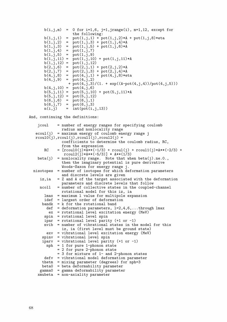
b(i,j,m) = 0 for i=1,6, j=1,jrange(i), m=1,12, except forthe following:

b(1,j,1) = pot(1,j,1) + pot(1,j,2)*A + pot(1,j,8)*etab(1,j,2) = pot(1,j,3) + pot(1,j,4)*Ab(1,j,3) = pot(1,j,5) + pot(1,j,6)*Ab(1,j,4) = pot(1,j,7)b(1,j,5) = pot(1,j,9)b(1,j,11) = pot(1,j,10) + pot(1,j,11)*Ab(1,j,12) = pot(1,j,12)b(2,j,6) = pot(2,j,1) + pot(2,j,2)*Ab(2,j,7) = pot(2,j,3) + pot(2,j,4)*Ab(4,j,8) = pot(4,j,1) + pot(4,j,8)*etab(4,j,9) = pot(4,j,2)

+ pot(4,j,3)/(1. + exp((A-pot(4,j,4))/pot(4,j,5)))b(4,j,10) = pot(4,j,6)b(5,j,11) = pot(5,j,10) + pot(5,j,11)*Ab(5,j,12) = pot(5,j,12)b(6,j,6) = pot(6,j,1)b(6,j,7) = pot(6,j,3)n(i,j) = int(pot(i,j,13))

And, continuing the definitions:

jcoul = number of energy ranges for specifying coulombradius and nonlocality range

ecoul(j) = maximum energy of coulomb energy range jrcoul0(j),rcoul(j),rcoul1(j),rcoul2(j) =

coefficients to determine the coulomb radius, RC,from the expression

RC = [rcoul0(j)*A**(-1/3) + rcoul(j) + rcoul1(j)*A**(-2/3) +rcoul2(j)*A**(-5/3)] * A**(1/3)

beta(j) = nonlocality range. Note that when beta(j).ne.0.,then the imaginary potential is pure derivativeWoods-Saxon for energy range j.

nisotopes = number of isotopes for which deformation parametersand discrete levels are given

iz,ia = Z and A of the target associated with the deformationparameters and discrete levels that follow

ncoll = number of collective states in the coupled-channelrotational model for this iz, ia

lmax = maximum l value for multipole expansionidef = largest order of deformation

bandk = k for the rotational banddef = deformation parameters, l=2,4,6,...through lmaxex = rotational level excitation energy (MeV)

spin = rotational level spinipar = rotational level parity (+1 or -1)nvib = number of vibrational states in the model for this

iz, ia (first level must be ground state)exv = vibrational level excitation energy (MeV)

spinv = vibrational level spiniparv = vibrational level parity (+1 or -1)

nph = 1 for pure 1-phonon state= 2 for pure 2-phonon state= 3 for mixture of 1- and 2-phonon states

defv = vibrational model deformation parameterthetm = mixing parameter (degrees) for nph=3beta0 = beta deformability parameter

gamma0 = gamma deformability parameterxmubeta = non-axiality parameter

68

ANNEX 5.B

REFERENCE NUMBERING SYSTEM

FOR RIPL OPTICAL MODEL POTENTIALS

DEFINITION: IREF = 1000*I + JREF

Table 5.4: Incident Particles (leading digit, I).

IREF I Particle1 - 3999 0 - 3 Neutrons

4000 - 5999 4 - 5 Protons6000 - 6999 6 Deuterons7000 - 7999 7 Tritons8000 - 8999 8 He-39000 - 9999 9 He-4

Table 5.5: Geographic Indicators (trailing 3 digits, JREF).

JREF Region1 - 99 Los Alamos National Laboratory (LANL)

100 - 199 Other U.S. laboratories, universities200 - 299 Japan, JAERI300 - 399 Russia400 - 499 Western Europe, JEF community500 - 599 China600 - 649 Former Soviet Union and Eastern Europe650 - 699 India, Pakistan700 - 799 Others800 - 999 Reserved

69

ANNEX 5.C

EXAMPLE OF A POTENTIAL

IN THE OPTICAL PARAMETER LIBRARY

5003E.D.Arthur and C.PhilisReport LA-8630-PR, p.2 (1980)Parameters are based on fits to 169Tm low-energy resonance data and totalcross sections, plus fits to 11-MeV neutron scattering on 165Ho. Lanemodel used to relate n and p potentials.

0.001 100.000067 69165 1691 1 1 0 01

100.0001.26000 0.00000+0 0.00000+0 0.00000+0 0.00000+0 0.00000+0 0.00000+0

0.00000+0 0.00000+0 0.00000+0 0.00000+00.63000 0.00000+0 0.00000+0 0.00000+0 0.00000+0 0.00000+0 0.00000+0

0.00000+0 0.00000+0 0.00000+0 0.00000+049.80000 -2.50000-1 0.00000+0 0.00000+0 0.00000+0 0.00000+0 1.60000+1

1.00000+0 0.00000+0 0.00000+0 0.00000+0 0.00000+0 0.00000+00.00000+0 0.00000+0 0.00000+0 0.00000+0 0.00000+0 0.00000+00.00000+0 0.00000+0 0.00000+0 0.00000+0 0.00000+0 0.00000+0

28.3001.26000 0.00000+0 0.00000+0 0.00000+0 0.00000+0 0.00000+0 0.00000+0

0.00000+0 0.00000+0 0.00000+0 0.00000+00.63000 0.00000+0 0.00000+0 0.00000+0 0.00000+0 0.00000+0 0.00000+0

0.00000+0 0.00000+0 0.00000+0 0.00000+00.00000 0.00000+0 0.00000+0 0.00000+0 0.00000+0 0.00000+0 0.00000+0

0.00000+0 0.00000+0 0.00000+0 0.00000+0 0.00000+0 0.00000+00.00000+0 0.00000+0 0.00000+0 0.00000+0 0.00000+0 0.00000+00.00000+0 0.00000+0 0.00000+0 0.00000+0 0.00000+0 0.00000+0

100.0001.26000 0.00000+0 0.00000+0 0.00000+0 0.00000+0 0.00000+0 0.00000+0

0.00000+0 0.00000+0 0.00000+0 0.00000+00.63000 0.00000+0 0.00000+0 0.00000+0 0.00000+0 0.00000+0 0.00000+0

0.00000+0 0.00000+0 0.00000+0 0.00000+0-1.00000 1.20000-1 0.00000+0 0.00000+0 0.00000+0 0.00000+0 0.00000+0

0.00000+0 0.00000+0 0.00000+0 0.00000+0 0.00000+0 0.00000+00.00000+0 0.00000+0 0.00000+0 0.00000+0 0.00000+0 0.00000+00.00000+0 0.00000+0 0.00000+0 0.00000+0 0.00000+0 0.00000+0

026.5001.26000 0.00000+0 0.00000+0 0.00000+0 0.00000+0 0.00000+0 0.00000+0

0.00000+0 0.00000+0 0.00000+0 0.00000+00.48000 0.00000+0 0.00000+0 0.00000+0 0.00000+0 0.00000+0 0.00000+0

0.00000+0 0.00000+0 0.00000+0 0.00000+05.02000 5.10000-1 0.00000+0 0.00000+0 0.00000+0 0.00000+0 8.00000+0

0.00000+0 0.00000+0 0.00000+0 0.00000+0 0.00000+0 0.00000+00.00000+0 0.00000+0 0.00000+0 0.00000+0 0.00000+0 0.00000+00.00000+0 0.00000+0 0.00000+0 0.00000+0 0.00000+0 0.00000+0

100.0001.26000 0.00000+0 0.00000+0 0.00000+0 0.00000+0 0.00000+0 0.00000+0

0.00000+0 0.00000+0 0.00000+0 0.00000+00.48000 0.00000+0 0.00000+0 0.00000+0 0.00000+0 0.00000+0 0.00000+0

0.00000+0 0.00000+0 0.00000+0 0.00000+08.93300 -9.20000-2 0.00000+0 0.00000+0 0.00000+0 0.00000+0 8.00000+0

0.00000+0 0.00000+0 0.00000+0 0.00000+0 0.00000+0 0.00000+00.00000+0 0.00000+0 0.00000+0 0.00000+0 0.00000+0 0.00000+00.00000+0 0.00000+0 0.00000+0 0.00000+0 0.00000+0 0.00000+0

1

70

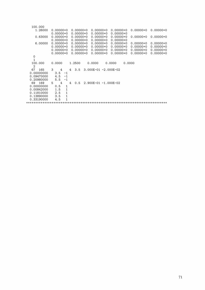
100.0001.26000 0.00000+0 0.00000+0 0.00000+0 0.00000+0 0.00000+0 0.00000+0

0.00000+0 0.00000+0 0.00000+0 0.00000+00.63000 0.00000+0 0.00000+0 0.00000+0 0.00000+0 0.00000+0 0.00000+0

0.00000+0 0.00000+0 0.00000+0 0.00000+06.00000 0.00000+0 0.00000+0 0.00000+0 0.00000+0 0.00000+0 0.00000+0

0.00000+0 0.00000+0 0.00000+0 0.00000+0 0.00000+0 0.00000+00.00000+0 0.00000+0 0.00000+0 0.00000+0 0.00000+0 0.00000+00.00000+0 0.00000+0 0.00000+0 0.00000+0 0.00000+0 0.00000+0

01

100.000 0.0000 1.2500 0.0000 0.0000 0.00002

67 165 3 4 4 3.5 3.000E-01 -2.000E-020.00000000 3.5 -10.09470000 4.5 -10.20980000 5.5 -169 169 5 4 4 0.5 2.900E-01 -1.000E-020.00000000 0.5 10.00842000 1.5 10.11810000 2.5 10.13890000 3.5 10.33190000 4.5 1

++++++++++++++++++++++++++++++++++++++++++++++++++++++++++++++++++++++++++++++

71

ANNEX 5.D

SUMMARY OF ENTRIES AND REFERENCES

INCLUDED IN THE RIPL-2 OPTICAL MODEL

POTENTIAL LIBRARY

This annex contains a summary of the optical model parameterizations that are in-cluded in the user version of the RIPL-2 optical model potential ibrary. The results aregiven in tabular form, with each entry summarized in a single line and with a completelist of the references included in the library (as defined by Ref. No.). The table andreference list were obtained using the om-summary.f computer code, which is includedin the RIPL-2/optical/om-get directory.

Lib. Inc. Model Disp Rel Z-Range A-Range E-Range Ref. FirstNo. Part. Type Pot Pot (MeV) No. Author

15 n spher. no no 6- 6 12- 12 0.0- 65.0 1 M.B.Chadwick2001 n spher. no yes 6-82 12-208 50.0-400.0 2 D.G.Madland

16 n spher. no no 7- 7 14- 14 0.0- 60.0 1 M.B.Chadwick136 n spher. no no 7- 7 14- 14 18.0- 60.0 3 M.S.Islam17 n spher. no no 8- 8 16- 16 0.0- 50.0 1 M.B.Chadwick

137 n spher. no no 8- 8 16- 16 18.0- 60.0 3 M.S.Islam101 n spher. no no 12-83 24-209 11.0- 11.0 4 J.C.Ferrer

1400 n spher. no yes 12-12 24- 24 0.0-200.0 5 A.J.Koning1401 n spher. no yes 12-12 26- 26 0.0-200.0 5 A.J.Koning

18 n spher. no no 13-13 27- 27 0.0- 20.0 6 R.C.Harper430 n spher. no no 13-82 27-208 0.1- 24.0 7 O.Bersillon117 n spher. no no 13-13 27- 27 0.0- 60.0 8 J.Petler243 n spher. no no 13-47 27-109 0.0- 80.0 9 N.Yamamuro419 n spher. yes no 13-13 27- 27 0.0-150.0 10 A. Molina

1402 n spher. no yes 13-13 27- 27 0.0-200.0 5 A.J.Koning2405 n spher. no yes 13-83 27-209 0.0-200.0 11 A.J.Koning242 n spher. no no 13-13 27- 27 0.0-250.0 12 Lee418 n spher. yes yes 13-13 27- 27 0.0-250.0 10 A. Molina

1403 n spher. no yes 14-14 28- 28 0.0-200.0 5 A.J.Koning1404 n spher. no yes 15-15 31- 31 0.0-200.0 5 A.J.Koning1405 n spher. no yes 16-16 32- 32 0.0-200.0 5 A.J.Koning1406 n spher. no yes 17-17 35- 35 0.0-200.0 5 A.J.Koning1408 n spher. no yes 18-18 40- 40 0.0-200.0 5 A.J.Koning1407 n spher. no yes 19-19 39- 39 0.0-200.0 5 A.J.Koning116 n spher. no no 20-83 40-209 0.0- 5.0 13 P.A.Moldauer401 n spher. no no 20-92 40-238 0.0- 25.0 14 D.Wilmore

2100 n spher. no no 20-83 40-209 10.0- 26.0 15 R.L.Varner100 n spher. no no 20-92 40-238 10.0- 50.0 16 F.D.Becchetti138 n spher. no no 20-20 40- 40 18.0- 60.0 3 M.S.Islam800 n spher. no no 20-83 40-210 0.0-155.0 17 C.A.Engelbrecht

1409 n spher. no yes 20-20 40- 40 0.0-200.0 5 A.J.Koning1410 n spher. no yes 21-21 45- 45 0.0-200.0 5 A.J.Koning133 n spher. no no 22-22 44- 50 0.1- 20.0 18 D.W.Muir

1411 n spher. no yes 22-22 48- 48 0.0-200.0 5 A.J.Koning134 n spher. no no 23-23 50- 51 0.1- 20.0 18 D.W.Muir404 n spher. no no 23-41 50- 95 0.0- 30.0 19 B.Strohmaier

72

1412 n spher. no yes 23-23 51- 51 0.0-200.0 5 A.J.Koning112 n spher. no no 24-24 50- 50 0.0-100.0 20 A.Prince114 n spher. no no 24-24 52- 52 0.0-100.0 20 A.Prince

1413 n spher. no yes 24-24 52- 52 0.0-200.0 5 A.J.Koning113 n spher. no no 24-24 53- 53 0.0-100.0 20 A.Prince115 n spher. no no 24-24 54- 54 0.0-100.0 20 A.Prince

1415 n spher. no yes 25-25 55- 55 0.0-200.0 5 A.J.Koning125 n spher. no no 26-26 54- 54 8.0- 14.0 21 S.M.El-Kadi428 n vibra. no no 26-26 54- 56 0.1- 14.0 22 J.P.Delaroche129 n spher. no no 26-29 54- 65 8.0- 30.0 21 S.M.El-Kadi130 n spher. no no 26-29 54- 65 8.0- 30.0 21 S.M.El-Kadi10 n spher. no no 26-26 54- 56 0.0- 52.0 23 E.D.Arthur

2101 n spher. no no 26-82 54-208 10.0- 80.0 24 R.L.Walter104 n spher. no no 26-26 54- 54 0.0-100.0 20 A.Prince

1414 n spher. no yes 26-26 54- 54 0.0-200.0 5 A.J.Koning126 n spher. no no 26-26 56- 56 8.0- 14.0 21 S.M.El-Kadi103 n spher. no no 26-26 56- 56 0.0-100.0 20 A.Prince

1416 n spher. no yes 26-26 56- 56 0.0-200.0 5 A.J.Koning105 n spher. no no 26-26 57- 57 0.0-100.0 20 A.Prince106 n spher. no no 26-26 58- 58 0.0-100.0 20 A.Prince11 n spher. no no 27-27 59- 59 0.0- 27.5 25 E.D.Arthur

1419 n spher. no yes 27-27 59- 59 0.0-200.0 5 A.J.Koning19 n spher. no no 28-28 58- 58 0.0- 20.0 6 R.C.Harper

131 n vibra. no no 28-28 58- 60 0.0- 80.0 26 P.P.Guss132 n spher. no no 28-28 58- 60 0.0- 80.0 26 P.P.Guss107 n spher. no no 28-28 58- 58 0.0-100.0 20 A.Prince

1417 n spher. no yes 28-28 58- 58 0.0-200.0 5 A.J.Koning108 n spher. no no 28-28 60- 60 0.0-100.0 20 A.Prince

1418 n spher. no yes 28-28 60- 60 0.0-200.0 5 A.J.Koning109 n spher. no no 28-28 61- 61 0.0-100.0 20 A.Prince110 n spher. no no 28-28 62- 62 0.0-100.0 20 A.Prince111 n spher. no no 28-28 64- 64 0.0-100.0 20 A.Prince127 n spher. no no 29-29 63- 63 8.0- 14.0 21 S.M.El-Kadi429 n vibra. no no 29-29 63- 65 0.1- 14.0 22 J.P.Delaroche

1420 n spher. no yes 29-29 63- 63 0.0-200.0 5 A.J.Koning128 n spher. no no 29-29 65- 65 8.0- 14.0 21 S.M.El-Kadi

1421 n spher. no yes 29-29 65- 65 0.0-200.0 5 A.J.Koning12 n spher. no no 30-30 57- 81 0.0- 20.0 27 P.G.Young

200 n spher. no no 31-69 69-146 0.0- 20.0 28 S.Igarasi240 n spher. no no 31-69 69-146 0.0- 20.0 29 S.Igarasi500 n spher. no no 31-31 69- 69 0.1- 20.0 30 Zhang

1422 n spher. no yes 31-31 69- 69 0.0-200.0 5 A.J.Koning1423 n spher. no yes 32-32 74- 74 0.0-200.0 5 A.J.Koning202 n spher. no no 33-37 61-107 0.0- 20.0 31 Japan

1424 n spher. no yes 33-33 75- 75 0.0-200.0 5 A.J.Koning1425 n spher. no yes 33-33 79- 79 0.0-200.0 5 A.J.Koning1426 n spher. no yes 34-34 80- 80 0.0-200.0 5 A.J.Koning501 n spher. no no 36-36 83- 83 0.1- 20.0 32 Cai502 n spher. no no 36-36 86- 86 0.1- 20.0 33 Cai503 n spher. no no 37-37 85- 85 0.1- 20.0 32 Cai

1427 n spher. no yes 37-37 85- 85 0.0-200.0 5 A.J.Koning203 n spher. no no 38-42 69-116 0.0- 20.0 31 Japan504 n spher. no no 38-38 88- 88 0.1- 20.0 32 Cai

1428 n spher. no yes 38-38 88- 88 0.0-200.0 5 A.J.Koning118 n spher. no no 39-51 85-125 0.0- 5.0 34 A.B.Smith505 n spher. no no 39-39 89- 89 0.1- 20.0 32 Cai13 n spher. no no 39-39 89- 89 0.0- 21.0 35 E.D.Arthur

1429 n spher. no yes 39-39 89- 89 0.0-200.0 5 A.J.Koning506 n spher. no no 39-39 91- 91 0.1- 20.0 36 Cai14 n spher. no no 40-40 90- 90 0.0- 20.0 37 E.D.Arthur

1430 n spher. no yes 40-40 90- 90 0.0-200.0 5 A.J.Koning2404 n spher. no no 40-40 90- 90 0.0-200.0 38 A.J.Koning1431 n spher. no yes 40-40 91- 91 0.0-200.0 5 A.J.Koning1432 n spher. no yes 40-40 92- 92 0.0-200.0 5 A.J.Koning1435 n spher. no yes 40-40 94- 94 0.0-200.0 5 A.J.Koning

73

20 n spher. no no 41-41 93- 93 0.0- 20.0 6 R.C.Harper507 n spher. no no 41-41 93- 93 0.1- 20.0 39 Rong

1434 n spher. no yes 41-41 93- 93 0.0-200.0 5 A.J.Koning508 n spher. no no 41-41 95- 95 0.1- 20.0 39 Rong422 n spher. no no 42-42 92-100 0.0- 20.0 40 Ch.Lagrange

1433 n spher. no yes 42-42 92- 92 0.0-200.0 5 A.J.Koning1436 n spher. no yes 42-42 94- 94 0.0-200.0 5 A.J.Koning509 n spher. no no 42-42 95- 95 0.1- 20.0 41 Cai

1437 n spher. no yes 42-42 96- 96 0.0-200.0 5 A.J.Koning510 n spher. no no 42-42 97- 97 0.1- 20.0 42 Cai511 n spher. no no 42-42 98- 98 0.1- 20.0 42 Cai

1438 n spher. no yes 42-42 98- 98 0.0-200.0 5 A.J.Koning512 n spher. no no 42-42 100-100 0.1- 20.0 33 Cai

1440 n spher. no yes 42-42 100-100 0.0-200.0 5 A.J.Koning204 n spher. no no 43-45 80-125 0.0- 20.0 31 Japan513 n spher. no no 43-43 99- 99 0.1- 20.0 36 Cai

1439 n spher. no yes 43-43 99- 99 0.0-200.0 5 A.J.Koning514 n spher. no no 44-44 99- 99 0.1- 20.0 43 Zhang515 n spher. no no 44-44 100-100 0.1- 20.0 43 Zhang516 n spher. no no 44-44 101-101 0.1- 20.0 44 Zhang517 n spher. no no 44-44 102-102 0.1- 20.0 43 Zhang518 n spher. no no 44-44 103-103 0.1- 20.0 44 Zhang519 n spher. no no 44-44 104-104 0.1- 20.0 43 Zhang520 n spher. no no 44-44 105-105 0.1- 20.0 43 Zhang521 n spher. no no 45-45 103-103 0.1- 20.0 43 Zhang

1441 n spher. no yes 45-45 103-103 0.0-200.0 5 A.J.Koning522 n spher. no no 45-45 105-105 0.1- 20.0 43 Zhang205 n spher. no no 46-48 89-134 0.0- 20.0 31 Japan523 n spher. no no 46-46 105-105 0.1- 20.0 45 Zhang

1442 n spher. no yes 46-46 106-106 0.0-200.0 5 A.J.Koning524 n spher. no no 46-46 108-108 0.1- 20.0 45 Zhang


1444 n spher. no yes 48-48 114-114 0.0-200.0 5 A.J.Koning206 n spher. no no 49-51 97-141 0.0- 20.0 31 Japan526 n spher. no no 49-49 115-115 0.1- 20.0 46 Zhang

1445 n spher. no yes 49-49 115-115 0.0-200.0 5 A.J.Koning1446 n spher. no yes 50-50 116-116 0.0-200.0 5 A.J.Koning1447 n spher. no yes 50-50 118-118 0.0-200.0 5 A.J.Koning1448 n spher. no yes 50-50 120-120 0.0-200.0 5 A.J.Koning1450 n spher. no yes 50-50 122-122 0.0-200.0 5 A.J.Koning1452 n spher. no yes 50-50 124-124 0.0-200.0 5 A.J.Koning527 n spher. no no 51-51 121-121 0.1- 20.0 46 Zhang


1451 n spher. no yes 51-51 123-123 0.0-200.0 5 A.J.Koning207 n spher. no no 52-54 103-150 0.0- 20.0 31 Japan

1454 n spher. no yes 52-52 128-128 0.0-200.0 5 A.J.Koning529 n spher. no no 52-52 130-130 0.1- 20.0 45 Zhang530 n spher. no no 53-53 127-127 0.1- 20.0 45 Zhang

1453 n spher. no yes 53-53 127-127 0.0-200.0 5 A.J.Koning531 n spher. no no 53-53 135-135 0.1- 20.0 45 Zhang532 n spher. no no 54-54 123-123 0.1- 20.0 47 Shen533 n spher. no no 54-54 124-124 0.1- 20.0 47 Shen534 n spher. no no 54-54 129-129 0.1- 20.0 48 Shen535 n spher. no no 54-54 131-131 0.1- 20.0 48 Shen536 n spher. no no 54-54 132-132 0.1- 20.0 48 Shen537 n spher. no no 54-54 134-134 0.1- 20.0 48 Shen538 n spher. no no 54-54 135-135 0.1- 20.0 48 Shen539 n spher. no no 54-54 136-136 0.1- 20.0 48 Shen208 n spher. no no 55-55 111-153 0.0- 20.0 31 Japan540 n spher. no no 55-55 133-133 0.1- 20.0 43 Zhang

1455 n spher. no yes 55-55 133-133 0.0-200.0 5 A.J.Koning541 n spher. no no 55-55 134-134 0.1- 20.0 43 Zhang542 n spher. no no 55-55 135-135 0.1- 20.0 43 Zhang

74

543 n spher. no no 55-55 137-137 0.1- 20.0 43 Zhang209 n spher. no no 56-56 112-154 0.0- 20.0 31 Japan544 n spher. no no 56-56 135-135 0.1- 20.0 43 Zhang545 n spher. no no 56-56 136-136 0.1- 20.0 43 Zhang546 n spher. no no 56-56 137-137 0.1- 20.0 43 Zhang547 n spher. no no 56-56 138-138 0.1- 20.0 43 Zhang

1456 n spher. no yes 56-56 138-138 0.0-200.0 5 A.J.Koning210 n spher. no no 57-58 117-156 0.0- 20.0 31 Japan548 n spher. no no 57-57 139-139 0.1- 20.0 43 Zhang


1458 n spher. no yes 58-58 140-140 0.0-200.0 5 A.J.Koning550 n spher. no no 58-58 141-141 0.1- 20.0 43 Zhang551 n spher. no no 58-58 142-142 0.1- 20.0 43 Zhang552 n spher. no no 58-58 144-144 0.1- 20.0 43 Zhang211 n spher. no no 59-59 119-160 0.0- 20.0 31 Japan553 n spher. no no 59-59 141-141 0.1- 20.0 47 Shen

1459 n spher. no yes 59-59 141-141 0.0-200.0 5 A.J.Koning212 n spher. no no 60-60 141-143 0.0- 20.0 31 Japan420 n vibra. no no 60-60 142-148 0.0- 15.0 49 G.Haouat554 n spher. no no 60-60 142-142 0.1- 20.0 47 Shen

1460 n spher. no yes 60-60 142-142 0.0-200.0 5 A.J.Koning555 n spher. no no 60-60 143-143 0.1- 20.0 47 Shen213 n spher. no no 60-60 144-148 0.0- 20.0 31 Japan556 n spher. no no 60-60 144-144 0.1- 20.0 47 Shen

1461 n spher. no yes 60-60 144-144 0.0-200.0 5 A.J.Koning557 n spher. no no 60-60 145-145 0.1- 20.0 47 Shen558 n spher. no no 60-60 146-146 0.1- 20.0 47 Shen559 n spher. no no 60-60 147-147 0.1- 20.0 47 Shen421 n CC rot. no no 60-60 148-150 0.0- 15.0 49 G.Haouat560 n spher. no no 60-60 148-148 0.1- 20.0 47 Shen214 n spher. no no 60-60 150-999 0.0- 20.0 31 Japan561 n spher. no no 60-60 150-150 0.1- 20.0 47 Shen215 n spher. no no 61-61 147-999 0.0- 20.0 31 Japan562 n spher. no no 61-61 147-147 0.1- 20.0 47 Shen563 n spher. no no 61-61 148-148 0.1- 20.0 47 Shen564 n spher. no no 61-61 149-149 0.1- 20.0 47 Shen216 n spher. no no 62-62 144-144 0.0- 20.0 31 Japan565 n spher. no no 62-62 144-144 0.1- 20.0 47 Shen217 n spher. no no 62-62 147-147 0.0- 20.0 31 Japan566 n spher. no no 62-62 147-147 0.1- 20.0 47 Shen123 n vibra. no no 62-62 148-150 0.0- 15.0 50 M.T.McEllistrem218 n spher. no no 62-62 148-148 0.0- 20.0 31 Japan567 n spher. no no 62-62 148-148 0.1- 20.0 47 Shen

1462 n spher. no yes 62-62 148-148 0.0-200.0 5 A.J.Koning219 n spher. no no 62-62 149-149 0.0- 20.0 31 Japan568 n spher. no no 62-62 149-149 0.1- 20.0 47 Shen124 n CC rot. no no 62-62 150-152 0.0- 15.0 50 M.T.McEllistrem220 n spher. no no 62-62 150-150 0.0- 20.0 31 Japan569 n spher. no no 62-62 150-150 0.1- 20.0 47 Shen570 n spher. no no 62-62 151-151 0.1- 20.0 47 Shen571 n spher. no no 62-62 152-152 0.1- 20.0 47 Shen572 n spher. no no 62-62 154-154 0.1- 20.0 47 Shen221 n spher. no no 63-63 151-999 0.0- 20.0 31 Japan573 n spher. no no 63-63 151-151 0.1- 20.0 51 Ge

2004 n CC rot. no no 63-63 151-153 0.0- 20.0 52 R.Macklin574 n spher. no no 63-63 153-153 0.1- 20.0 51 Ge575 n spher. no no 63-63 154-154 0.1- 20.0 51 Ge576 n spher. no no 63-63 155-155 0.1- 20.0 51 Ge222 n spher. no no 64-64 133-171 0.0- 20.0 31 Japan577 n spher. no no 64-64 152-152 0.1- 20.0 47 Shen578 n spher. no no 64-64 154-154 0.1- 20.0 47 Shen579 n spher. no no 64-64 155-155 0.1- 20.0 47 Shen580 n spher. no no 64-64 156-156 0.1- 20.0 47 Shen581 n spher. no no 64-64 157-157 0.1- 20.0 47 Shen

75

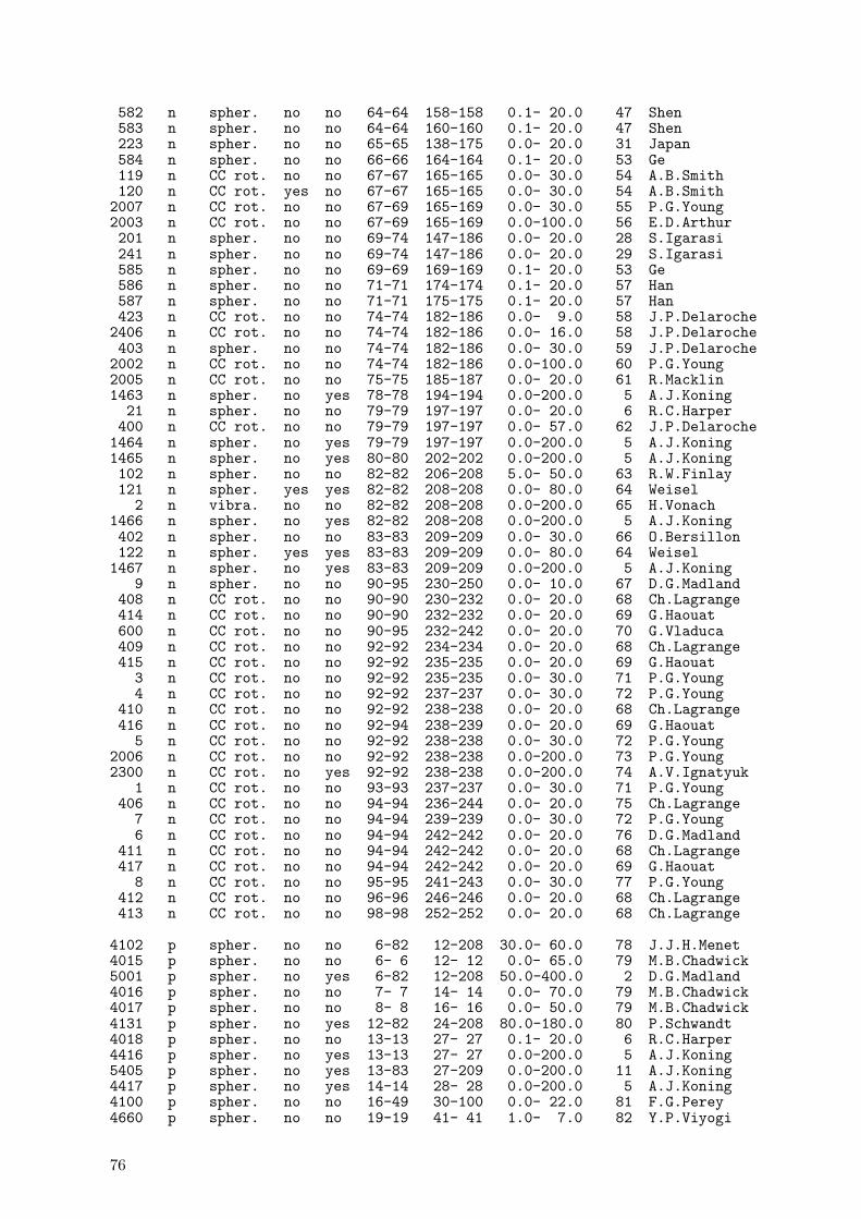
582 n spher. no no 64-64 158-158 0.1- 20.0 47 Shen583 n spher. no no 64-64 160-160 0.1- 20.0 47 Shen223 n spher. no no 65-65 138-175 0.0- 20.0 31 Japan584 n spher. no no 66-66 164-164 0.1- 20.0 53 Ge119 n CC rot. no no 67-67 165-165 0.0- 30.0 54 A.B.Smith120 n CC rot. yes no 67-67 165-165 0.0- 30.0 54 A.B.Smith

2007 n CC rot. no no 67-69 165-169 0.0- 30.0 55 P.G.Young2003 n CC rot. no no 67-69 165-169 0.0-100.0 56 E.D.Arthur201 n spher. no no 69-74 147-186 0.0- 20.0 28 S.Igarasi241 n spher. no no 69-74 147-186 0.0- 20.0 29 S.Igarasi585 n spher. no no 69-69 169-169 0.1- 20.0 53 Ge586 n spher. no no 71-71 174-174 0.1- 20.0 57 Han587 n spher. no no 71-71 175-175 0.1- 20.0 57 Han423 n CC rot. no no 74-74 182-186 0.0- 9.0 58 J.P.Delaroche

2406 n CC rot. no no 74-74 182-186 0.0- 16.0 58 J.P.Delaroche403 n spher. no no 74-74 182-186 0.0- 30.0 59 J.P.Delaroche

2002 n CC rot. no no 74-74 182-186 0.0-100.0 60 P.G.Young2005 n CC rot. no no 75-75 185-187 0.0- 20.0 61 R.Macklin1463 n spher. no yes 78-78 194-194 0.0-200.0 5 A.J.Koning

21 n spher. no no 79-79 197-197 0.0- 20.0 6 R.C.Harper400 n CC rot. no no 79-79 197-197 0.0- 57.0 62 J.P.Delaroche

1464 n spher. no yes 79-79 197-197 0.0-200.0 5 A.J.Koning1465 n spher. no yes 80-80 202-202 0.0-200.0 5 A.J.Koning102 n spher. no no 82-82 206-208 5.0- 50.0 63 R.W.Finlay121 n spher. yes yes 82-82 208-208 0.0- 80.0 64 Weisel

2 n vibra. no no 82-82 208-208 0.0-200.0 65 H.Vonach1466 n spher. no yes 82-82 208-208 0.0-200.0 5 A.J.Koning402 n spher. no no 83-83 209-209 0.0- 30.0 66 O.Bersillon122 n spher. yes yes 83-83 209-209 0.0- 80.0 64 Weisel

1467 n spher. no yes 83-83 209-209 0.0-200.0 5 A.J.Koning9 n spher. no no 90-95 230-250 0.0- 10.0 67 D.G.Madland

408 n CC rot. no no 90-90 230-232 0.0- 20.0 68 Ch.Lagrange414 n CC rot. no no 90-90 232-232 0.0- 20.0 69 G.Haouat600 n CC rot. no no 90-95 232-242 0.0- 20.0 70 G.Vladuca409 n CC rot. no no 92-92 234-234 0.0- 20.0 68 Ch.Lagrange415 n CC rot. no no 92-92 235-235 0.0- 20.0 69 G.Haouat

3 n CC rot. no no 92-92 235-235 0.0- 30.0 71 P.G.Young4 n CC rot. no no 92-92 237-237 0.0- 30.0 72 P.G.Young

410 n CC rot. no no 92-92 238-238 0.0- 20.0 68 Ch.Lagrange416 n CC rot. no no 92-94 238-239 0.0- 20.0 69 G.Haouat

5 n CC rot. no no 92-92 238-238 0.0- 30.0 72 P.G.Young2006 n CC rot. no no 92-92 238-238 0.0-200.0 73 P.G.Young2300 n CC rot. no yes 92-92 238-238 0.0-200.0 74 A.V.Ignatyuk

1 n CC rot. no no 93-93 237-237 0.0- 30.0 71 P.G.Young406 n CC rot. no no 94-94 236-244 0.0- 20.0 75 Ch.Lagrange

7 n CC rot. no no 94-94 239-239 0.0- 30.0 72 P.G.Young6 n CC rot. no no 94-94 242-242 0.0- 20.0 76 D.G.Madland

411 n CC rot. no no 94-94 242-242 0.0- 20.0 68 Ch.Lagrange417 n CC rot. no no 94-94 242-242 0.0- 20.0 69 G.Haouat

8 n CC rot. no no 95-95 241-243 0.0- 30.0 77 P.G.Young412 n CC rot. no no 96-96 246-246 0.0- 20.0 68 Ch.Lagrange413 n CC rot. no no 98-98 252-252 0.0- 20.0 68 Ch.Lagrange

4102 p spher. no no 6-82 12-208 30.0- 60.0 78 J.J.H.Menet4015 p spher. no no 6- 6 12- 12 0.0- 65.0 79 M.B.Chadwick5001 p spher. no yes 6-82 12-208 50.0-400.0 2 D.G.Madland4016 p spher. no no 7- 7 14- 14 0.0- 70.0 79 M.B.Chadwick4017 p spher. no no 8- 8 16- 16 0.0- 50.0 79 M.B.Chadwick4131 p spher. no yes 12-82 24-208 80.0-180.0 80 P.Schwandt4018 p spher. no no 13-13 27- 27 0.1- 20.0 6 R.C.Harper4416 p spher. no yes 13-13 27- 27 0.0-200.0 5 A.J.Koning5405 p spher. no yes 13-83 27-209 0.0-200.0 11 A.J.Koning4417 p spher. no yes 14-14 28- 28 0.0-200.0 5 A.J.Koning4100 p spher. no no 16-49 30-100 0.0- 22.0 81 F.G.Perey4660 p spher. no no 19-19 41- 41 1.0- 7.0 82 Y.P.Viyogi

76

4101 p spher. no no 20-83 40-209 10.0- 50.0 83 F.D.Becchetti5100 p spher. no no 20-83 40-209 16.0- 65.0 15 R.L.Varner4418 p spher. no yes 20-20 40- 40 0.0-200.0 5 A.J.Koning4651 p spher. no no 20-20 48- 48 3.0- 5.0 84 S.Kailas4662 p spher. no no 20-20 48- 48 1.0- 7.0 82 Y.P.Viyogi4108 p spher. no no 20-82 48-208 25.0- 45.0 85 D.M.Patterson4650 p spher. no no 21-21 45- 45 3.0- 5.0 84 S.Kailas4661 p spher. no no 21-21 45- 45 1.0- 7.0 82 Y.P.Viyogi4663 p spher. no no 22-22 49- 49 1.0- 7.0 82 Y.P.Viyogi4652 p spher. no no 23-23 51- 51 3.0- 5.0 84 S.Kailas4664 p spher. no no 23-23 51- 51 1.0- 7.0 82 Y.P.Viyogi4653 p spher. no no 24-24 54- 54 3.0- 5.0 84 S.Kailas4000 p spher. no no 25-26 54- 56 0.0- 28.0 23 E.D.Arthur4665 p spher. no no 25-25 55- 55 1.0- 7.0 82 Y.P.Viyogi5101 p spher. no no 26-82 54-208 10.0- 80.0 86 R.L.Walter4419 p spher. no yes 26-26 54- 54 0.0-200.0 5 A.J.Koning4420 p spher. no yes 26-26 56- 56 0.0-200.0 5 A.J.Koning4001 p spher. no no 26-27 59- 59 0.0- 23.0 87 E.D.Arthur4654 p spher. no no 27-27 59- 59 3.0- 5.0 84 S.Kailas4666 p spher. no no 27-27 59- 59 1.0- 7.0 82 Y.P.Viyogi4019 p spher. no no 28-28 58- 58 0.1- 20.0 6 R.C.Harper4421 p spher. no yes 28-28 58- 58 0.0-200.0 5 A.J.Koning4422 p spher. no yes 28-28 60- 60 0.0-200.0 5 A.J.Koning4655 p spher. no no 28-28 61- 61 3.0- 5.0 84 S.Kailas4667 p spher. no no 28-28 61- 61 1.0- 7.0 82 Y.P.Viyogi4423 p spher. no yes 28-28 62- 62 0.0-200.0 5 A.J.Koning4425 p spher. no yes 28-28 64- 64 0.0-200.0 5 A.J.Koning4424 p spher. no yes 29-29 63- 63 0.0-200.0 5 A.J.Koning4656 p spher. no no 29-29 65- 65 3.0- 5.0 84 S.Kailas4668 p spher. no no 29-29 65- 65 1.0- 7.0 82 Y.P.Viyogi4669 p spher. no no 30-30 68- 68 1.0- 7.0 82 Y.P.Viyogi4657 p spher. no no 31-31 71- 71 3.0- 5.0 84 S.Kailas4670 p spher. no no 31-31 71- 71 1.0- 7.0 82 Y.P.Viyogi4658 p spher. no no 33-33 75- 75 3.0- 5.0 84 S.Kailas4671 p spher. no no 33-33 75- 75 1.0- 7.0 82 Y.P.Viyogi4659 p spher. no no 34-34 80- 80 3.0- 5.0 84 S.Kailas4672 p spher. no no 34-34 80- 80 1.0- 7.0 82 Y.P.Viyogi4002 p spher. no no 38-38 88- 89 0.0- 21.0 35 E.D.Arthur4109 p spher. no no 39-39 89- 89 1.0- 7.0 88 C.H.Johnson4673 p spher. no no 39-39 89- 89 1.0- 7.0 82 Y.P.Viyogi4003 p spher. no no 39-39 89- 89 0.0- 21.0 35 E.D.Arthur4426 p spher. no yes 40-40 90- 90 0.0-200.0 5 A.J.Koning5404 p spher. no no 40-40 90- 90 0.0-200.0 38 A.J.Koning4125 p spher. no no 40-40 92- 92 2.0- 7.0 89 D.S.Flynn4126 p spher. no no 40-40 94- 94 2.0- 7.0 89 D.S.Flynn4127 p spher. no no 40-40 96- 96 2.0- 7.0 89 D.S.Flynn4110 p spher. no no 41-41 93- 93 1.0- 7.0 88 C.H.Johnson4674 p spher. no no 41-41 93- 93 1.0- 7.0 82 Y.P.Viyogi4020 p spher. no no 41-41 93- 93 0.1- 20.0 6 R.C.Harper4128 p spher. no no 42-42 95- 95 2.0- 7.0 89 D.S.Flynn4675 p spher. no no 42-42 96- 96 1.0- 7.0 82 Y.P.Viyogi4129 p spher. no no 42-42 98- 98 2.0- 7.0 89 D.S.Flynn4676 p spher. no no 42-42 98- 98 1.0- 7.0 82 Y.P.Viyogi4130 p spher. no no 42-42 100-100 2.0- 7.0 89 D.S.Flynn4111 p spher. no no 45-45 103-103 1.0- 7.0 88 C.H.Johnson4677 p spher. no no 45-45 103-103 1.0- 7.0 82 Y.P.Viyogi4112 p spher. no no 46-46 105-105 1.0- 7.0 88 C.H.Johnson4678 p spher. no no 46-46 105-105 1.0- 7.0 82 Y.P.Viyogi4113 p spher. no no 47-47 107-107 1.0- 7.0 88 C.H.Johnson4679 p spher. no no 47-47 107-107 1.0- 7.0 82 Y.P.Viyogi4114 p spher. no no 47-47 109-109 1.0- 7.0 88 C.H.Johnson4680 p spher. no no 47-47 109-109 1.0- 7.0 82 Y.P.Viyogi4115 p spher. no no 48-48 110-110 1.0- 7.0 88 C.H.Johnson4681 p spher. no no 48-48 110-110 1.0- 7.0 82 Y.P.Viyogi4116 p spher. no no 48-48 111-111 1.0- 7.0 88 C.H.Johnson

77

4117 p spher. no no 48-48 113-113 1.0- 7.0 88 C.H.Johnson4118 p spher. no no 48-48 114-114 1.0- 7.0 88 C.H.Johnson4119 p spher. no no 49-49 115-115 1.0- 7.0 88 C.H.Johnson4682 p spher. no no 49-49 115-115 1.0- 7.0 82 Y.P.Viyogi4120 p spher. no no 50-50 116-116 1.0- 7.0 88 C.H.Johnson4683 p spher. no no 50-50 120-120 1.0- 7.0 82 Y.P.Viyogi4427 p spher. no yes 50-50 120-120 0.0-200.0 5 A.J.Koning4121 p spher. no no 50-50 122-122 1.0- 7.0 88 C.H.Johnson4122 p spher. no no 50-50 124-124 1.0- 7.0 88 C.H.Johnson4684 p spher. no no 50-50 124-124 1.0- 7.0 82 Y.P.Viyogi4123 p spher. no no 52-52 128-128 1.0- 7.0 88 C.H.Johnson4685 p spher. no no 52-52 128-128 1.0- 7.0 82 Y.P.Viyogi4124 p spher. no no 52-52 130-130 1.0- 7.0 88 C.H.Johnson4686 p spher. no no 52-52 130-130 1.0- 7.0 82 Y.P.Viyogi5004 p CC rot. no no 63-63 151-153 0.0- 20.0 52 R.Macklin5003 p CC rot. no no 67-69 165-169 0.0-100.0 56 E.D.Arthur5406 p CC rot. no no 74-74 182-186 0.0- 16.0 58 J.P.Delaroche5002 p CC rot. no no 74-74 182-186 0.0-100.0 60 P.G.Young5005 p CC rot. no no 75-75 185-187 0.0- 20.0 61 R.Macklin4004 p CC rot. no no 79-79 197-197 0.0- 57.0 90 P.G.Young4428 p spher. no yes 82-82 208-208 0.0-200.0 5 A.J.Koning4429 p spher. no yes 83-83 209-209 0.0-200.0 5 A.J.Koning5006 p CC rot. no no 92-92 238-238 0.0-200.0 73 P.G.Young5300 p CC rot. no yes 92-92 238-238 0.0-200.0 74 A.V.Ignatyuk

6400 d spher. no no 6-82 12-208 20.0-100.0 91 J.Bojowald6100 d spher. no no 20-83 40-209 8.0- 13.0 92 J.M.Lohr6101 d spher. no no 20-82 40-208 11.0- 27.0 93 C.M.Perey6112 d spher. no no 20-20 40- 40 11.8- 90.0 94 W.W.Daehnick6113 d spher. no no 28-28 58- 58 11.8- 90.0 94 W.W.Daehnick6114 d spher. no no 40-40 90- 90 11.8- 90.0 94 W.W.Daehnick6115 d spher. no no 50-50 120-120 11.8- 90.0 94 W.W.Daehnick6116 d spher. no no 82-82 208-208 11.8- 90.0 94 W.W.Daehnick

7100 t spher. no no 20-82 40-208 1.0- 40.0 95 F.D.Becchetti

8100 3He spher. no no 20-82 40-208 1.0- 40.0 95 F.D.Becchetti8101 3He spher. no no 20-20 40- 40 21.0- 84.0 96 H.H.Chang8102 3He spher. no no 28-28 58- 58 22.0- 84.0 96 H.H.Chang

9100 4He spher. no no 8-82 16-208 1.0- 25.0 97 L.McFadden9600 4He spher. no no 8-96 16-250 1.0- 73.0 98 V.Avrigeanu9101 4He spher. no no 10-92 20-235 1.0- 46.0 99 J.R.Huizenga9018 4He spher. no no 13-13 27- 27 0.1- 20.0 6 R.C.Harper9000 4He spher. no no 13-26 27- 56 1.0-100.0 100 E.D.Arthur9400 4He spher. no no 20-45 40-100 1.0- 30.0 19 B.Strohmaier9401 4He spher. no no 22-30 37- 86 20.0- 30.0 101 O.F.Lemos9001 4He spher. no no 27-27 59- 59 1.0-100.0 102 E.D.Arthur9019 4He spher. no no 28-28 58- 58 0.1- 20.0 6 R.C.Harper9020 4He spher. no no 41-41 93- 93 0.1- 20.0 6 R.C.Harper

78

REFERENCES TO ANNEX 5.D

[1] CHADWICK, M.B., YOUNG, P.G., Nucl. Sci. Eng. 123 (1996) 17.

[2] MADLAND, D.G., OECD/NEA Specialists’ Meeting Nucleon-Nucleus OpticalModel to 200 MeV, Paris (1997) 129.

[3] ISLAM, M.S., FINLAY, R.W., PETLER, J.S., RAPAPORT, J., ALARCON, R.,Phys. Med. Biol. 33 (1988) 315.

[4] FERRER, J.C., CARLSON, J.D., RAPAPORT, J., Nucl. Phys. A275 (1977) 325.

[5] KONING, A.J., DELAROCHE, J.P., Nucl. Phys. A713 (2003) 231.

[6] HARPER, R.C., ALFORD, W.L., J. Phys. G: Nucl. Phys. 8 (1982) 153.

[7] BERSILLON, O., CINDRO, Fifth Int. Sym. Interactions of Fast Neutrons withNuclei, Gaussig (1975).

[8] PETLER, J., ISLAM, M.S., FINLAY, R.W., Phys. Rev. C32 (1985) 673.

[9] YAMAMURO, N., Int. Conf. Nucl. Data for Science and Technol., Mito (1988)489.

[10] MOLINA, A., CAPOTE, R., QUESADA, J.M., LOZANO, M., Phys. Rev. C65(2002) 034616.

[11] KONING, A.J., DELAROCHE, J.P., Nucl. Phys. A713 (2003) 231.

[12] LEE, Y-O., CHANK, J., FUKAHORI, T., CHIBA, S., J. Nucl. Sci. Technol. 36(1999) 1125.

[13] MOLDAUER, P.A., Nucl. Phys. 47 (1963) 65.

[14] WILMORE, D., HODGSON, P.E., Nucl. Phys. 55 (1964) 673.

[15] VARNER, R.L., THOMPSON, W.J., MCABEE, T.L., LUDWIG, E.J., CLEGG,T.B., Phys. Rep. 201 (1991) 57.

[16] BECCETTI Jr., F.D., GREENLEES, G.W., Phys. Rev. 182 (1969) 1190.

[17] ENGELBRECHT, C.A., FIEDELDEY, H., Ann. Phys. 42 (1967) 262.

[18] MUIR, D.W., ARTHUR, E.D., J. Nucl. Mat. 122/123 (1984) 1058.

[19] STROHMAIER, B., UHL, M., REITER, W., “Neutron Cross Section Calculationsfor 52Cr, 55Mn, 56Fe, and 58,60Ni”, IAEA Advisory Group Meeting on Nuclear Datafor Radiation Damage Assessment and Related Safety Aspects, Vienna, Austria,October 1981, INDC(NDS)-128, IAEA Vienna (1982).

[20] PRINCE, A., Int. Conf. Nucl. Data, Antwerp (1982).

[21] EL-KADI, S.M., NELSON, C.E., PURSER, F.O., WALTER, R.L., BEYERLE,A., GOULD, C.R. SEAGONDOLLA, L.W., Nucl. Phys. A390 (1982) 509.

79

[22] DELAROCHE, J.P., EL-KADI, S.M., GUSS, P.P., FLOYD, C.E., WALTER, R.L.,Nucl. Phys. A390 (1982) 541.

[23] ARTHUR, E.D., YOUND, P.G., LA-UR-95-3654 (1995), BNL-NCS-51245 (1980)731, LA-8626-MS (1980).

[24] WALTER, R.L., GUSS, P.P., Rad. Effects 95 (1986) 73.

[25] ARTHUR, E.D., YOUNG, P.G., MATTHES, W., BNL-51245 (1980) 751; Nucl.Sci. Eng. 124 (1996) 271.

[26] GUSS, P.P., BYRD, R.C., FLOYD, C.E., HOWELL, C.R., MURPHY, K., TUN-GATE, G., DELAROCHE, J.P., Nucl. Phys. A438 (1985) 187.

[27] YOUNG, P.G., RUTHERFORD, D., IAEA-TECDOC-483 (1988) 167.

[28] IGARASI, S., Japan Atomic Energy Research Institute, JAERI 1228 (1973) 41.

[29] IGARASI, S., JAERI-M 5752 (1974).

[30] ZHANG SONGBAI, China Nuclear Data Center, Communication of Nuclear DataProgress, No. 21 (1999) 52.

[31] Japan Atomic Energy Research Institute (JAERI), JNDC FP Nucl. Data WG.

[32] CAI CHONGHAI, Nankai University, Tianjin, P.R. China, Communication of Nu-clear Data Progress, No. 21 (1999) 40.

[33] CAI CHONGHAI, Nankai University, Tainjin, P.R. China, private communication.

[34] SMITH, A.B., GUENTHER, P.T., WHALEN, J.F., Nucl. Phys. A415 (1984) 1.

[35] ARTHUR, E.D., Nucl. Sci. Eng. 76 (1980) 137.

[36] CAI CHONGHAI, Nankai University, Tianjin, P.R. China, private communication.

[37] ARTHUR, E.D., Nucl. Sci. Eng. 76 (1980) 137; LA-UR-94-3104 (1994).

[38] KONING, A.J., VAN WIJK, J.J., DELAROCHE, J.P., OECD/NEA SpecialistMtg. Nucleon-Nucleus Opt. Mod. to 200 MeV, Paris (1997) 111.

[39] RONG JIAN, ZHANG ZHENGJUN, China Nuclear Data Center, private commu-nication.

[40] LAGRANGE, Ch., Specialist Meeting Neutron Data for Structural Materials, Geel(1977).

[41] CAI CHONGHAI, Nankai University, Tainjin, P.R. China, private communication.

[42] CAI CHONGHAI, GE ZHIGANG, China Nuclear Data Center, private communi-cation.

[43] ZHANG ZHENGJUN, Phys. Dept. of Northwest University, Xian, private commu-nication.

80

[44] ZHANG ZHENGJUN, GE ZHIGANG, China Nuclear Data Center, private com-munication.

[45] ZHANG ZHENGJUN, GE ZHIGANG, China Nuclear Data Center, private com-munication.

[46] ZHANG ZHENGJUN, et al., Communication of Nuclear Data Progress, No. 20(1998) 77.

[47] SHEN QINGBIAO, China Nuclear Data Center, private communication.

[48] SHEN QINGBIAO, ZHANG ZHENGJUN, China Nuclear Data Center, privatecommunication.

[49] HAOUAT, G., LACHKAR, J., LAGRANGE, Ch., MCELLISTREM, M.T.,PATIN, Y., SHAMU, R.E., SIGAUD, J., Phys. Rev. C20 (1979) 78.

[50] McELLISTREM, M.T., SHAMU, R.E., LACHKAR, J., HAOUAT, G., LA-GRANGE, Ch., PATIN, Y., SIGAUD, J., COCU, F., Phys. Rev. C15 (1977)927.

[51] GE ZHIAGANG, China Nuclear Data Center, Communication of Nuclear DataProgress, No. 21 (1999) 35.

[52] MACKLIN, R., YOUNG, P.G., Nucl. Sci. Eng. 95 (1987) 189.

[53] GE ZHIAGANG, China Nuclear Data Center, private communication.

[54] SMITH, A.B., ANL/NDM-151 (December 2000).

[55] YOUNG, P.G., LA-UR (1997).

[56] ARTHUR, E.D., PHILIS, C., LA-8630-PR (1980) 2.

[57] HAN YINLU, China Nuclear Data Center, private communication.

[58] DELAROCHE, J.P., HAOUAT, G., LACHKAR, J., PATIN, Y., SIGAUD, J.,CHARDINE, J., Phys. Rev. C23 (1981) 136.

[59] DELAROCHE, J.P., et al., Int. Conf. Nucl. Data, Knoxville, TN (1978).

[60] YOUNG, P.G., ARTHUR, E.D., BOZIAN, M., ENGLAND, T.R., HALE, G.M.,LABAUVE, R.J., LITTLE, R.C., et al., LA-11753-MS (1990); see also LA-8630-PR, (1980) 2.

[61] MACKLIN, R., YOUNG, P.G., Nucl. Sci. Eng. 97 (1987) 239.

[62] DELAROCHE, J.P., Proc. Int. Conf. Neut. Phys. for Reactors, Harwell, UK, 25-29Sept. 1978.

[63] FINLAY, R.W., ANNAND, J.R.M., CHEEMA, T.S. RAPAPORT, J., DIETRICH,F.S., Phys. Rev. C30 (1984) 796.

[64] WEISEL, G.J., TORNOW, W., HOWELL, C.R., FELSHER, P.D., ALOHALI,M., ROBERTS, M.L., DAS, R.K., WALTER, R.L., Phys. Rev. C54 (1996) 2410.

81

[65] VONACH, H., PAVLIK, A., CHADWICK, M.B., HAIGHT, R.C., NELSON, R.O.,WENDER, S.A., YOUNG, P.G., Phys. Rev. C50 (1994) 1952.

[66] BERSILLON, O., CEA-N-2284 (1982) 130; see also NEANDC-222.

[67] MADLAND, D.G., YOUNG, P.G., Int. Conf. Neut. Phys. for Reactors, Harwell,UK, 25-29 Sept. 1978.

[68] LAGRANGE, Ch., NEANDC(E)228, INDC(FR)-56 (1982).

[69] HAOUAT, G., LACHKAR, J., LAGRANGE, Ch., Nucl. Sci. Eng. 81 (1982) 491.

[70] VLADUCA, G., TUDORA, A., SIN, M., Rom. J. Phys., 41, no. 7-8 (1996) 515.

[71] YOUNG, P.G., ARTHUR, E.D., in Proc. Int. Conf. Nucl. Data Sci. Tech., Julich(1992) 894.

[72] YOUNG, P.G., ARTHUR, E.D., LA-UR-91-1424, 894 (1992).

[73] YOUNG, P.G., LA-11972-PR (1990) 9.

[74] IGNATYUK, A.V., LUNEV, V.P., SHUBIN, Yu.N., GAI, E.V., TITARENKO,N.N., VENTURA, A., GUDOWSKI, W., Nucl. Sci. Eng. 136 (2000) 340.

[75] LAGRANGE, Ch., CEA-N-1970, NEANDC(E) 179, INDC(FR)-16 (1977).

[76] MADLAND, D.G., YOUNG, P.G., LA-7533-MS (1978).

[77] YOUNG, P.G., ARTHUR, E.D., LA-UR-95-3654, paper at CRP RIPL Meeting,Vienna, 30 Oct. - 3 Nov. 1995.

[78] MENET, J.J.H., GROSS, E.E., MALANIFY, J.J., ZUCKER, A., Phys. Rev. C4(1971) 1114.

[79] CHADWICK, M.B., YOUNG, P.G., Proc. Int. Particle Therapy Meeting andPTCOG XXIV, 24-26 April 1996, Detroit, Michigan, USA.

[80] SCHWANDT, P., MEYER, H.O., JACOBS, W.W., BACHER, A.D., VIGDOR,S.E., KAITCHUCK, M.D., et al., Phys. Rev. C26 (1982) 55.

[81] PEREY, F.G., Phys. Rev. 131 (1963) 745.

[82] VIYOGI, Y.P., Ph.D Thesis, Calcutta University (1983).

[83] BECCHETTI Jr., F.D., GREENLEES, G.W., Phys. Rev. 182 (1969) 1190.

[84] KAILAS, S., MEHTA, M.K., GUPTA, S.K., VIYOGI, Y.P., GANGULY, N.K.,Phys. Rev. C20 (1979) 1272;MEHTA, M.K., KAILAS, S., Pramana. J. Phys. 27 (1986) 139.

[85] PATTERSON, D.M., DOERING, R.R., GALONSKY, A., Nucl. Phys. A263(1976) 261.

[86] WALTER, R.L., GUSS, P.P., Rad. Effects 95 (1986) 73.

82

[87] ARTHUER, E.D., YOUNG, P.G., MATTHES, W., BNL-51245 (1980) 751; Nucl.Sci. Eng. 124 (1996) 271.

[88] JOHNSON, C.H., GALONSKY, A., KERNELL, R.L., Phys. Rev. Lett. 39 (1977)1604; Phys. Rev. C20 (1979) 2052.

[89] FLYNN, D.S., HERSHBERGER, R.L., GABBARD, F., Phys. Rev. C31 (1985)87.

[90] YOUNG, P.G., ARTHUR, E.D., LA-UR-84-2767 (1984); LA-UR-94-3104 (1994).

[91] BOJOWALD, J., MACHNER, H., NANN, H., OELERT, W., ROGGE, M.,TUREK, P., Phys. Rev. C38 (1988) 1153.

[92] LOHR, J.M., HAEBERLI, W., Nucl. Phys. A232 (1974) 381.

[93] PEREY, C.M., PEREY, F.G., Phys. Rev. 132 (1963) 755.

[94] DAEHNICK, W.W., CHILDS, J.D., VRCELJ, Z., Phys. Rev. C21 (1980) 2253.

[95] BECCHETTI Jr., F.D., GREENLEES, G.W., Annual Report, J.H. Williams Lab-oratory, University of Minnesota (1969).

[96] CHANG, H.H., RIDLEY, B.W., BRAID, T.H., CONLON, T.W., GIBSON, E.F.,KING, N.S.P., Nucl. Phys. A297 (1978) 105.

[97] MCFADDEN, L., SATCHLER, G.R., Nucl. Phys. 84 (1966) 177.

[98] AVRIGEANU, V., HODGSON, P.E., AVRIGEANU, M., OUNP-94-02 (1994);Phys. Rev. C49 (1994) 2136.

[99] HUIZENGA, J.R., IGO, G., Nucl. Phys. 29 (1962) 462.

[100] ARTHUR, E.D., YOUNG, P.G., LA-8636-MS(ENDF-304) (1980).

[101] LEMOS, O.F., Orsay, Series A, No. 136 (1972).

[102] ARTHUR, E.D., YOUNG, P.G., MATTHES, W., BNL-51245, 751 (1980).

83

6 NUCLEAR LEVEL DENSITIES

Coordinators: A.V. Ignatyuk and R. Capote

Summary

Level densities are key ingredients of the statistical theory of nuclear reactions. Practicalformalisms of nuclear level densities and their parameterization are considered in thischapter. The total level densities required for the statistical calculations of reaction crosssections at low and intermediate energies are described in Section 6.1. Then, the partial(particle-hole) level densities needed as input to the extremely useful pre-equilibriummodel of nuclear reactions are discussed in Section 6.2. The fission level densities requiredfor the statistical calculations of the fission cross sections are considered separately inChapter 8, together with the corresponding fission barriers.

The RIPL-2 library includes a FORTRAN code written by Avrigeanu for variousFermi-gas single-particle models in the equidistant spacing approximation, including pair-ing and shell effects within the closed-form treatments. A FORTRAN code produced byCapote and Pedrosa has also been adopted which uses a microscopic theory based on aconvolution of shell-model single-particle states with BCS pairing.

The statistical properties of excited nuclear levels have been a matter of concern andstudy for many years. One of the basic statistical properties of these levels is theirdensity, for which the Fermi-gas and constant temperature models are frequently usedwith input parameters obtained from fitting certain experimental data. However, thephysical assumptions underlying these models are not sufficiently sophisticated to accountproperly for variations of level densities over a wide energy interval from the ground stateto well above the neutron separation energy. This is not surprising as these models wereformulated more than fifty years ago, in the infancy of such concepts of nuclear physics.

Some of the most important concepts upon which our current understanding of thestructure of low-lying nuclear levels is based include shell effects, pairing correlations andcollective phenomena. All these concepts have been incorporated into the generalizedsuper-fluid model developed by many authors over the last 30 years. The phenomenolog-ical versions of this model are convenient for the analysis of experimental data and havebeen developed intensively over recent years.

For practical applications of the statistical models, it is very important to obtainparameters of the level densities from reliable experimental data. The cumulative numbersof low-lying levels and the average distances between neutron resonances are usually

85

used for this purpose. The systematics of the level density parameters developed underthe RIPL project are discussed below together with recommendations regarding theirapplication to different tasks.

6.1 Total level densities

6.1.1 Composite Gilbert-Cameron model

Simple analytical expressions for the excited state density ρ(U) of a nucleus with a givenexcitation energy U and level density ρ(U, J) of a nucleus with a given angular momentumJ were obtained by Bethe on the basis of the Fermi-gas model [6.1]:

ρ(U) =

√π

12a1/4U5/4exp(2

√aU),

ρ(U, J) =2J + 1

2√

2πσ3ρ(U) exp

[−(J + 1/2)2

2σ2

], (6.1)

in which a = π2g/6 is the level density parameter proportional to the single-particle statedensity g near the Fermi energy, and σ2 is the spin cutoff parameter.

For the Fermi-gas model, the state equations determining the dependence of the ex-citation energy U , the entropy S and other thermodynamic functions of a nucleus ontemperature t have simple forms:

U = at2, S = 2at, σ2 =< m2 > gt, (6.2)

where < m2 > is the mean square value of the angular momentum projections for thesingle-particle states around the Fermi energy, which may also be associated with themoment of inertia of a heated nucleus I = g < m2 >. There are obvious connectionsbetween the thermodynamic functions (Eqs. 6.2) and the state and level densities (Eq.6.1).

The main parameters of the Fermi-gas model may be estimated rather simply usingthe semi-classical approximation:

a = 2(

π

3

)4/3 m0r20

h2 A(1 + βsA−1/3), (6.3)

I0 =2

5

m0r20

h2 A5/3, (6.4)

where m0 is the nucleon mass, r0 is the nuclear radius parameter, A is the mass number andβs defines the surface component of the single-particle level density. Eq. 6.4 correspondsto the rigid-body value of the nuclear moment of inertia, and differences between varioussemi-classical determinations of the level density parameters (Eq. 6.3) are mainly due tothe large uncertainties in the existing evaluations for βs.

The most direct information on the level density of highly-excited nuclei is obtainedfrom the average parameters of neutron resonances, which have been analyzed by many

86

authors [6.2–6.11]. For the majority of nuclei the observed resonances correspond to s-neutrons, and therefore the value of the average spacings D0 is related to the level densityof the compound nucleus by the relationships:

(D0)−1 =

{12[ρ(Bn + ∆E/2, I0 + 1/2) + ρ(Bn + ∆E/2, I0 − 1/2)] for I0 �= 0,

12ρ(Bn + ∆E/2, 1/2) for I0 = 0,

(6.5)

were Bn is the neutron binding energy, ∆E is the energy interval for which the resonancesare being examined, I0 is the target nucleus spin, and the coefficient 1/2 before the sumtakes into account that s-neutrons form resonances only of a particular parity. If necessary,resonances for p-neutrons can be considered in a similar way.

The experimental values of D0 are normally used as source data, from which themagnitude of the level density parameter can be derived by means of Eqs. 6.1 and 6.5.Many authors have carried out such an analysis [6.5, 6.7, 6.8]. The regular differencesof the level densities for even-even, odd and odd-odd nuclei analogous to the even-odddifferences of the nuclear masses have been already noted in the early systematics of theexperimental data. The so-called effective excitation energy is normally introduced totake this effect into account:

U∗ = U −

⎧⎪⎪⎪⎨⎪⎪⎪⎩

δZ + δN for even− evenδZ for even ZδN for even N0 for odd − odd

(6.6)

where δI is the corresponding phenomenological correction for even-odd differences ofnuclear binding energies.

Data on the cumulative numbers of low-lying nuclear levels are also very importantfor level density analyses. The observed energy dependence of the cumulative number oflevels can be described rather well by the function [6.3, 6.5]:

N(U) = exp[(U − U0)/T ], (6.7)

where U0 and T are free parameters determined by fitting corresponding data. N(U) isrelated to the level density by the equation:

ρlev(U) =dN

dU=

1

Texp [(U − U0)/T ] , (6.8)

in which the parameter T corresponds simply to a nuclear temperature. Since the valueof this parameter is assumed to be constant over the energy range considered, Eq. 6.8 iscalled the constant temperature model.

A description of the level density for the whole range of excitation energies is obtainedby combining the low-energy dependent Eq. 6.8 with the high-energy dependence pre-dicted by the Fermi-gas model. The link between the parameters of both models can befound by imposing the continuity of level density and the first derivative at some matchingenergy

Ux = U0 + T ln ρfg(Ux),1

T=

√a

U∗x

− 3

2U∗x

, (6.9)

where U∗x is the effective matching energy that includes the pairing corrections (Eq. 6.6).

87

Analysis of the experimental data within this phenomenological approach was carriedout initially by Gilbert and Cameron [6.5], and the parameters obtained by differentauthors in the subsequent analyzes of experimental data are reported in the RIPL-1Handbook [6.12]. A rather simple systematic relationship has been proposed for the leveldensity parameter:

a

A= 0.0088 (S(Z) + S(N)) + Q(Z, N), (6.10)

where S(I) are the shell corrections for protons and neutrons, respectively, and Q(Z, N) =0.12 for deformed nuclei (54 < Z < 78, 86 < N < 122, and 86 < Z < 122, 130 < N <182), and Q(Z, N) = 0.142 for other nuclei considered as spherical. Tables of the shellcorrections and the corresponding pairing contribution corrections are given in the RIPL-1data files.

Values of the a-parameters depend to some extent on the determination of the spincutoff parameter. Early systematics used a value of < m2 >= 0.146A2/3, which corre-sponds to mean-square averaging of the proton and neutron angular momenta projectionsover all single-particle levels occupied in the ground state of a nucleus [6.5, 6.7]. Lateranalyses used more correct values < m2 >= 0.24A2/3, or the rigid body values of themoment of inertia. These differences in the choice of the spin cutoff parameters, as wellas some variations in the even-odd corrections to the excitation energies, should be bornein mind when comparing the a-parameters obtained by different authors.

Adjusted tables of the shell and pairing corrections were proposed in Refs. [6.13-6.15].The systematics of the a-parameter differ from Eq. 6.10 only in the numerical values ofthe coefficients and a slightly different definition of the functions Q(Z, N). Parametersderived by the Beijing group [6.15] are based on rather recent compilations of the neutronresonance densities, and were included in the beijing gc.dat file of the RIPL-1 project asrecommended data.

Revision of the low-lying data and the neutron resonance spacings described in Chap-ters 3 and 4 requires an updating of the level density parameters. Level density param-eters obtained for the updated resonance spacings are shown in Fig. 6.1 in comparisonwith the results of previous analyses [6.11, 6.15]. We have used the pairing correctionsδ = n12A−1/2 with n = 2 for even-even nuclei, n = 1 for odd nuclei and n = 0 for odd-odd nuclei. Such a definition of the pairing corrections is used in the Myers-Swiateckimass formula, and reproduces the averaged behavior of the corrections reported in Refs.[6.5, 6.15]. The same corrections were also used in Ref. [6.11]. Agreement of the RIPL-2results with the parameters obtained by Iljinov et al [6.11] is good for most nuclei, andtheir differences from the Beijing data arise from the slightly different pairing correctionsand the updated values of the resonance spacings.

The level density parameters obtained from the resonance spacing analysis were matchedwith the level density of low-lying levels by solving Eqs. 6.7 and 6.9 for the cumulativenumbers N0 of low-lying levels and the corresponding excitation energies U0 as definedin the recommendations of Chapter 3. Fig. 6.2 shows the nuclear temperatures T , theenergy shifts U0 , and the matching energies Ux. Generally, the present results are close tosimilar results of previous analyses considered in the RIPL-1 Handbook [6.12]. However,the matching equations for the level densities (Eqs. 6.9) set some limitations on the tem-peratures and the energy shifts, resulting in differences between the values derived fromthe matching conditions and the same parameters estimated from the analysis of low-lying

88

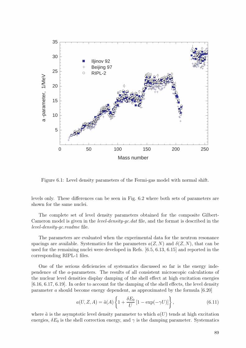
0 50 100 150 200 250

5

10

15

20

25

30

35

Iljinov 92 Beijing 97 RIPL-2

Mass number

a -p

aram

eter

, 1/

MeV

Figure 6.1: Level density parameters of the Fermi-gas model with normal shift.

levels only. These differences can be seen in Fig. 6.2 where both sets of parameters areshown for the same nuclei.

The complete set of level density parameters obtained for the composite Gilbert-Cameron model is given in the level-density-gc.dat file, and the format is described in thelevel-density-gc.readme file.

The parameters are evaluated when the experimental data for the neutron resonancespacings are available. Systematics for the parameters a(Z, N) and δ(Z, N), that can beused for the remaining nuclei were developed in Refs. [6.5, 6.13, 6.15] and reported in thecorresponding RIPL-1 files.

One of the serious deficiencies of systematics discussed so far is the energy inde-pendence of the a-parameters. The results of all consistent microscopic calculations ofthe nuclear level densities display damping of the shell effect at high excitation energies[6.16, 6.17, 6.19]. In order to account for the damping of the shell effects, the level densityparameter a should become energy dependent, as approximated by the formula [6.20]

a(U, Z, A) = a(A)

{1 +

δE0

U[1− exp(−γU)]

}, (6.11)

where a is the asymptotic level density parameter to which a(U) tends at high excitationenergies, δE0 is the shell correction energy, and γ is the damping parameter. Systematics

89

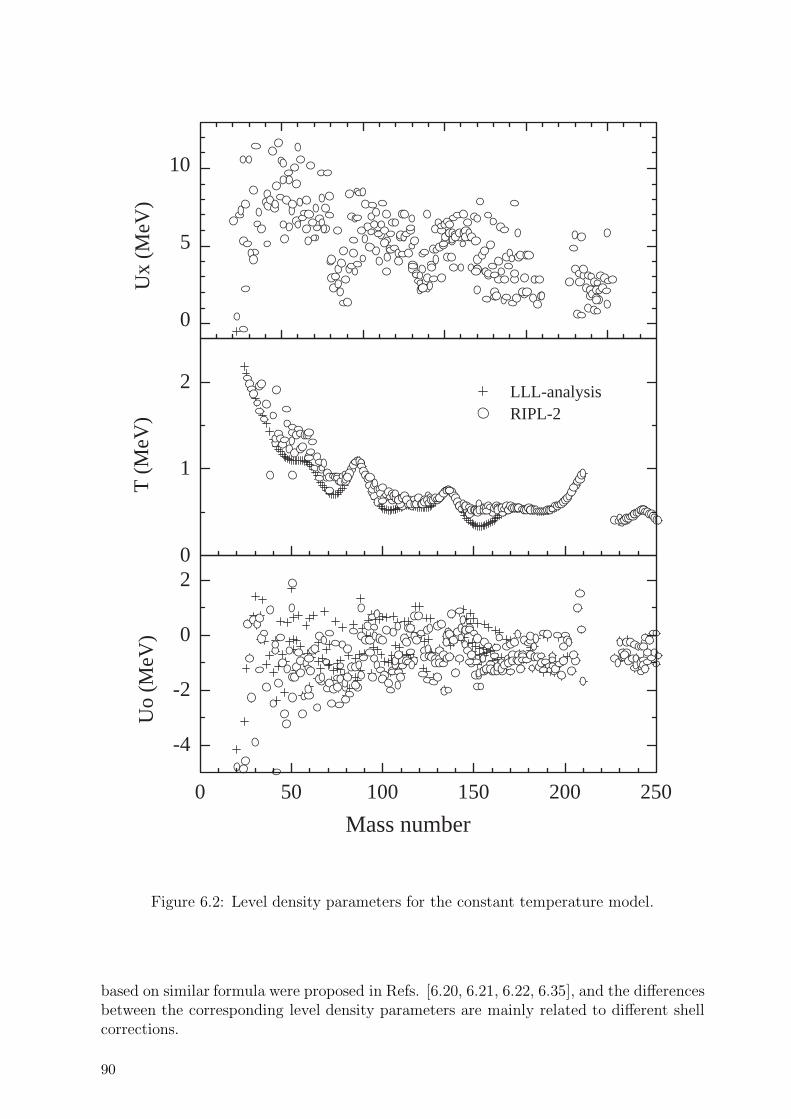
0 50 100 150 200 250

-4

-2

0

2

Mass number

Uo

(MeV

)

0

1

2

T (

MeV

)

LLL-analysis RIPL-2

0

5

10U

x (M

eV)

Figure 6.2: Level density parameters for the constant temperature model.

based on similar formula were proposed in Refs. [6.20, 6.21, 6.22, 6.35], and the differencesbetween the corresponding level density parameters are mainly related to different shellcorrections.

90

Shell corrections are usually determined as

δE0 = Mexp(Z, A)−Mld(Z, A, β), (6.12)

where Mexp is the experimental value of the mass defect, and Mld is the liquid-dropcomponent of the mass formula [6.23]. Differences between the various approximationsare mainly related to the liquid-drop component; if the liquid-drop model formula forspherical nuclei are adopted in Eq. 6.12, the shell corrections coincide with the microscopicenergies considered in Chapter 2. However, some authors prefer to include the deformationenergies within the liquid-drop component of Eq. 6.12 [6.23]. Such a consistent definitionof the shell corrections is important for the analysis of equilibrium deformations of highlyexcited nuclei [6.18], but differences in the shell correction estimations are less essentialfor the systematics of the level density parameters.

Fig. 6.3 shows the shell corrections corresponding to the most widely used massformula [6.5, 6.23, 6.24] for the nuclei considered above. If these corrections are takentogether with the a-parameter values for the neutron binding energies (Fig. 6.1), theasymptotic level density parameters can be derived on the basis of Eq. 6.11. Using thesemi-classical formula for the asymptotic and damping parameters

a = αA + βA2/3, γ = γ0/A1/3, (6.13)

and the Myers-Swiatecki shell corrections, the following coefficients (in units of MeV−1)were obtained from a least-squares fit of the a-parameters:

α = 0.0959 ± 0.0005, β = 0.1468 ± 0.0035, γ0 = 0.325± 0.015 (6.14)

Another mass-dependence formula for the asymptotic level density parameter is preferablefor the Moller-Nix shell corrections because of their large values for the actinides:

a = αA + βA2, [with γ = γ0/A1/3] (6.15)

with the corresponding coefficients:

α = 0.1125 ± 0.0005, β = (1.22± 0.11)10−4, γ0 = 0.325± 0.015. (6.16)

Deviations of the a-parameters included in the RIPL-2 level-densities-gc.dat file fromthe parameters calculated on the basis of systematics are shown in Fig. 6.4 for both sets ofshell corrections. Standard deviations are equal to 0.0613 for the systematics using Myers-Swiatecki corrections, and 0.0649 for Moller-Nix corrections. These results show thatboth systematics have approximately equal accuracy, and can be used for the evaluationof unknown level density parameters with expected uncertainties of about 6.5%. TheMyers-Swiatecki shell corrections for about 8000 nuclei are given in the shellcor-ms.datfile, while those of Moller-Nix are listed in the masses/mass-frdm95.dat file discussed inChapter 2.

The systematics of the constant temperature model parameters were discussed in Ref.[6.25], in which the nuclear temperature used in Eq. 6.7 was approximated by the formula

T = 17.60A−0.699√

1 + γδE0, (6.17)

91

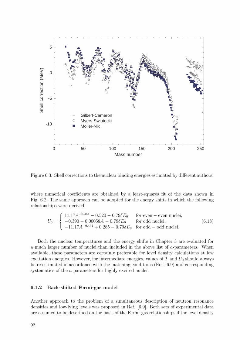
0 50 100 150 200 250

-10

-5

0

5

Gilbert-Cameron Myers-Swiatecki Moller-Nix

Mass number

She

ll co

rrec

tion

(MeV

)

Figure 6.3: Shell corrections to the nuclear binding energies estimated by different authors.

where numerical coefficients are obtained by a least-squares fit of the data shown inFig. 6.2. The same approach can be adopted for the energy shifts in which the followingrelationships were derived:

U0 =

⎧⎪⎨⎪⎩

11.17A−0.464 − 0.520− 0.79δE0 for even− even nuclei,−0.390− 0.00058A − 0.79δE0 for odd nuclei,−11.17A−0.464 + 0.285− 0.79δE0 for odd − odd nuclei.

(6.18)

Both the nuclear temperatures and the energy shifts in Chapter 3 are evaluated fora much larger number of nuclei than included in the above list of a-parameters. Whenavailable, these parameters are certainly preferable for level density calculations at lowexcitation energies. However, for intermediate energies, values of T and U0 should alwaysbe re-estimated in accordance with the matching conditions (Eqs. 6.9) and correspondingsystematics of the a-parameters for highly excited nuclei.

6.1.2 Back-shifted Fermi-gas model

Another approach to the problem of a simultaneous description of neutron resonancedensities and low-lying levels was proposed in Ref. [6.9]. Both sets of experimental dataare assumed to be described on the basis of the Fermi-gas relationships if the level density

92

0 50 100 150 200 250

-0,3

-0,2

-0,1

0,0

0,1

0,2

0,3

MN shell corrections MS shell corrections

Mass number

(aex

p-a

calc)/

aex

p

Figure 6.4: Deviations between the level density parameters derived from the resonancespacing analysis and the systematics based on the shell-correction formula (Moller-Nix(MN) and Myers-Swiatecki (MS)).

parameter a and the excitation energy shift δeff are considered as free parameters foreach nucleus. Since for odd-odd nuclei the resulting displacement is negative, the aboveapproach is known as the back-shifted Fermi-gas model. Since in this approach the Fermi-gas formula are applied to a rather low excitation energies, a more accurate estimation oftemperature is used

U − δeff = at2 − t,

and the temperature is usually added to the excitation energy in the dominator of Eq.6.1 [6.9].

Results of the corresponding analysis of the neutron resonance densities and low-lying nuclear levels are shown in Fig. 6.5. Due to the change in the determination ofthe effective excitation energies, the values obtained for the a-parameters are somewhatlower than those shown in Fig. 6.1. However, shell effects in the mass dependence ofthe a-parameter remain essentially the same. Differences between parameters obtained inRIPL-1 [6.12] and RIPL-2 reflect the improvements achieved for both sets of experimentaldata: neutron resonance spacings and cumulative numbers of low-lying levels.

Spin cutoff parameters are usually determined on the basis of the evaluation of themoment of inertia to give the rigid-body value and half this value. The results of thespin-distribution analysis of low-lying levels considered in Chapter 3 are shown in Fig. 6.6.The half-rigid-body value of the moment of inertia is in reasonable agreement with the

93

0 50 100 150 200 250

-4

-2

0

2

Mass number

ener

gy s

hift

(M

eV)

0

5

10

15

20

25

30

a-pa

ram

eter

(M

eV-1)

Huang 91 RIPL-2

Figure 6.5: Level density parameters in the back-shifted Fermi-gas model.

available data, but because of the large uncertainties more accurate spin cutoff parametersare difficult to estimate. Accordingly, the half-rigid-body moments of inertia were usedfor the evaluation of the a-parameters presented in Fig. 6.5.

The complete set of level density parameters obtained for the back-shifted Fermi-gasmodel is given in the level-density-bsfg.dat file, and the format is described in the level-density-bsfg.readme file.

94

50 100 150 200 2500

2

4

6

8

[S

pin

cut-

off]

1/2

Mass number

sigma FoT/2

Figure 6.6: Spin cutoff parameters obtained from the analysis of low-lying levels in com-parison with calculations using the half-rigid-body value of the moment of inertia.

Systematics for the level density parameters of the BSFG model were developed inRef. [6.26] on the basis of Eq. 6.11, which differs from the above for the Gilbert-Cameronmodel through mainly the pairing corrections. These corrections were taken to be equalto (δZ +δN )/2 for even-even nuclei, 0 for odd nuclei, and −(δZ +δN)/2 for odd-odd nuclei.Whereas for the Moller-Nix shell corrections and the asymptotic level density parametergiven by Eqs. 6.13, the following coefficients (in MeV−1) were obtained:

α = 0.1337, β = −0.06571, γ = 0.04884. (6.19)

We performed similar analysis for the a-parameters shown in Fig. 6.5. The Myers-Swiatecki shell corrections were used, the asymptotic level density parameter was takenas Eq. 6.13, and the pairing corrections were chosen to be equal to 12/A1/2 for even-evennuclei, 0 for odd nuclei, and −12/A1/2 for odd-odd nuclei. The following coefficients (inMeV−1) were obtained:

α = 0.0904± 0.0005, β = 0.0373 ± 0.0035, γ0 = 0.325± 0.015. (6.20)

For the Moller-Nix shell corrections and the asymptotic level density parameter definedby Eqs. 6.15 these coefficients are

α = 0.0883± 0.012, β = (1.03± 0.84)10−4, γ0 = 0.325± 0.015. (6.21)

95

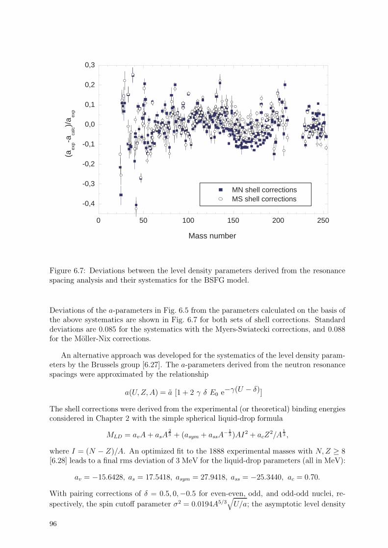
0 50 100 150 200 250

-0,4

-0,3

-0,2

-0,1

0,0

0,1

0,2

0,3

MN shell corrections MS shell corrections

Mass number

(aex

p-aca

lc)/

aex

p

Figure 6.7: Deviations between the level density parameters derived from the resonancespacing analysis and their systematics for the BSFG model.

Deviations of the a-parameters in Fig. 6.5 from the parameters calculated on the basis ofthe above systematics are shown in Fig. 6.7 for both sets of shell corrections. Standarddeviations are 0.085 for the systematics with the Myers-Swiatecki corrections, and 0.088for the Moller-Nix corrections.

An alternative approach was developed for the systematics of the level density param-eters by the Brussels group [6.27]. The a-parameters derived from the neutron resonancespacings were approximated by the relationship

a(U, Z, A) = a [1 + 2 γ δ E0 e−γ(U − δ)]

The shell corrections were derived from the experimental (or theoretical) binding energiesconsidered in Chapter 2 with the simple spherical liquid-drop formula

MLD = avA + asA23 + (asym + assA

− 13 )AI2 + acZ

2/A13 ,

where I = (N − Z)/A. An optimized fit to the 1888 experimental masses with N, Z ≥ 8[6.28] leads to a final rms deviation of 3 MeV for the liquid-drop parameters (all in MeV):

av = −15.6428, as = 17.5418, asym = 27.9418, ass = −25.3440, ac = 0.70.

With pairing corrections of δ = 0.5, 0,−0.5 for even-even, odd, and odd-odd nuclei, re-

spectively, the spin cutoff parameter σ2 = 0.0194A5/3√

U/a; the asymptotic level density

96

0.1

1

10

Dth

/ D

exp

BSFG

0.1

1

10

50 100 150 200 250

Dth

/ D

exp

A

HFBCS

Figure 6.8: Comparison between theoretical Dth and experimental Dexp values of the s-neutron resonance spacings. The theoretical predictions are obtained with the analyticalBSFG formula given in the text (upper panel) and the HFBCS-based model (lower panel).

parameters of Eqs. 6.13, can be obtained from a least-squares fit of the updated s-neutronresonance spacings Dexp to give the following coefficients (in MeV−1):

α = 0.1012, β = 0.0356, γ = 0.030. (6.22)

Ratios Dth/Dexp of the theoretical and experimental resonance spacings are shown inFig. 6.8. The root mean square deviation factor can be used to estimate the overalldeviation with respect to the experimental data:

frms = exp

[1

Ne

Ne∑i=1

ln2 Dith

Diexp

]1/2

,

where Ne is the number of nuclei considered. The present parameterization describes theexperimental data with a deviation frms = 1.78 that is comparable with the deviationfactor frms = 1.48 obtained for the more complex parameterization of the BSFG modelparameters in Ref. [6.26]. Results of microscopic calculations of resonance spacings arealso shown in Fig. 6.8 for comparison, and will be considered later.

Note that the BSFG model can diverge for the very low excitation energies for even-even and odd nuclei. So the BSFG model should be combined with the constant tempera-ture model for excitation energies below the accepted upper boundary of low-lying levels.

97

Of course, the nuclear temperatures and energy shifts for such a low-energy approach willbe rather different from those considered for the Gilbert-Cameron model (see above).

6.1.3 Generalized superfluid model

On the basis of all results considered above, we can conclude that the Fermi-gas and con-stant temperature models provide us with comparatively simple and convenient formulafor parameterizing experimental data on nuclear level densities. However, these models donot give any explanation for the shifts of excitation energies and shell changes of the leveldensity parameters. An interpretation of these effects must be obtained on the basis ofmore rigorous models that take into consideration shell inhomogeneities of single-particlelevel spectra, and the superfluid and collective effects produced by the residual interactionof nucleons. A detailed discussion of such models can be found in Ref. [6.18]. However,rigorous microscopic methods to calculate level densities are extremely laborious whichlimits their application to experimental data analyses. Thus, there is a need to develop aconsistent phenomenological description of nuclear level densities that takes into accountthe basic ideas of microscopic approaches to the structure of highly excited nuclear levels,while being sufficiently simple and convenient for broad application.

The influence of the super-conductive pairing correlations on nuclear properties canbe characterized by the value of the correlation functions (∆0τ), which determine directlythe even-odd differences in the nuclear binding energies and the energy gap of 2∆0τ inthe spectrum of quasi-particle excitations in even-even nuclei. The critical temperaturetc of the phase transition from a super-conductive (superfluid) to a normal state is alsorelated to the correlation function

tc = 0.567∆0. (6.23)

The excitation energy corresponding to the critical temperature may be expressed as:

Uc =π2

6gt2c +

1

4g∆2

0 − n∆0, (6.24)

where n = 0, 1 and 2 for even-even, odd and odd-odd nuclei, respectively.

Above the critical energy the level density and other nuclear thermodynamic functionscan be described by the Fermi-gas relationship in which the effective excitation energy isdefined as

U∗ = U − Econd, (6.25)

where Econd is the condensation energy that determines a reduction of the nuclear groundstate energy due to the pairing correlations

Econd =1

4g∆2

0 − n∆0. (6.26)

Below the phase transition point (Eq. 6.23) the expressions for the thermodynamicfunctions of a nucleus are rather complex, and will not be considered here. Completeexpressions can be found in Refs. [6.18, 6.29, 6.30], and the corresponding codes wereincluded in the RIPL-1 files.

98

If coherent collective effects are included to accommodate excited level structure, thenuclear level density may be expressed as

ρ(U) = ρqp(U)Kvibr(U)Krot(U), (6.27)

where ρqp is the level density due to quasi-particle excitations only, and Kvibr and Krot arethe corresponding enhancement coefficients due to vibrational and rotational excitations,respectively.

Rotational enhancement of the level density in the adiabatic approximation dependson the nuclear shape symmetry, and can be written as [6.31]

Krot =

{1 for spherical nuclei,I⊥t for deformed nuclei,

(6.28)

where I⊥ is the moment of inertia relative to the perpendicular axis. This formula isobtained if mirror and axial symmetry of a deformed nuclei is assumed. The most stablenuclei of the rare-earth elements (150 ≤ A ≤ 190) and the actinides A ≥ 230 have thisshape. Rotational enhancement of the level density becomes greater for non-axial forms[6.31].

The vibrational enhancement coefficient is determined in the microscopic approach bythe relationship

Kvibr =∏i

[1− exp(−ω0

i /t)

1− exp(−ωi/t)

]gi

, (6.29)

where ωi is the energy of the vibrational excitations, ω0i is the energy of the corresponding

quasi-particle excitation, and gi is the degeneracy of such excitations. The presenceof quasi-particle energies in Eq. 6.29 accounts to some extent for non-adiabatic effectsin excited nuclei. Due to symmetry constrains imposed on the nuclear Hamiltonian,the rotational and vibrational excitations become connected in a consistent microscopicapproach [6.18]. As a result, the calculated collective enhancement coefficients are alwaysreduced in comparison to the adiabatic estimation.

The adiabatic estimation of Krot increases the nuclear level densities by a factor of 50-100 compared to calculations based on quasi-particle excitations alone. Increases of leveldensities due to vibrational excitations will only be appreciable for low-energy excitationswith ωi < 1-2 MeV.

Over the previous twenty years, some microscopic models have been developed to con-sider collective effects in highly excited nuclei. The results of all these models demonstratethe damping of level density enhancement factors with increase of excitation energy. Onthe basis of the level density calculations within the SU-3 model (oscillator mean fieldwith the quadrupole-quadrupole interaction between particles), Hansen and Jensen [6.32]obtained the empirical function

Krot(U) =Kadiab

rot (U)

1 + exp[(U − Ur)/dr ], (6.30)

that describes the damping of rotational enhancement factors. The parameters of thisformula were estimated as

Ur = 120A1/3β22 MeV, dr = 1400A−2/3β2

2 MeV, (6.31)

99

where β2 is the quadrupole deformation parameter. Some other phenomenological de-scriptions for the damping enhancement factor were discussed in Refs. [6.33, 6.34, 6.35].All such descriptions include at least one or two parameters that can fluctuate from onenucleus to another. Rather large uncertainties exist in estimates of the collective dampingenhancement, and unfortunately we have no reliable experimental data that could be usedfor a crucial test of the various model predictions.

The vibrational enhancement of the level density can be approximated by the equation

Kvibr = exp[δS − (δU/t)], (6.32)

where δS and δU are changes in the entropy and excitation energy, respectively, that resultfrom the vibrational modes. These changes are described by the Bose gas relationships:

δS =∑

i

(2λi + 1)[(1 + ni) ln(1 + ni)− ni lnni],

δU =∑

i

(2λi + 1)ωini, (6.33)

where ωi are the energies, λi are the multipolarities, and ni are the occupation numbersfor vibrational excitations at a given temperature. The disappearance of collective en-hancement of the level density at high temperatures can be taken into account by definingthe occupation numbers in terms of the equation:

ni =exp(−γi/2ωi)

exp(ωi/t)− 1, (6.34)

where γi are the spreading widths of the vibrational excitations. This spreading of collec-tive excitations in nuclei should be similar to the zero-sound damping in a Fermi liquid,and the corresponding width can be written as

γi = C(ω2i + 4π2t2). (6.35)

A value of C = 0.0075A1/3 MeV−1 was obtained from the systematics of the neutronresonance densities of medium-weight nuclei [6.36]. This analysis adopted experimentalvalues for the energies of the first 2+ excitation, and ω = 50A−2/3 MeV for the octupoleexcitations. Due to higher energies, the influence of the latter is much weaker than forthe quadrupole excitations.

The shell inhomogeneities of single-particle level spectra result in a particular form ofenergy dependence of the level density parameter a(U): shell effects become weaker withincreasing excitation energy, and at sufficiently high energies the dependence of parametera on the mass number tends to the semi-classical value (Eq. 6.3). This important behaviorof the level density parameter was used in defining the systematics of the Fermi-gas modelparameters (Eq. 6.11). Similar equations for the GSM model [6.29] can be written as

a(U, Z, A) =

{a(A) [1 + δE0 f(U∗)/U∗] for U ≥ Uc,ac(Uc, Z, A) for U < Uc.

(6.36)

An additional shift of the excitation energies

Ueff = U∗ + δshift

100

0 50 100 150 200 250-2

-1

0

1

Mass number

Shif

t (M

eV)

0

5

10

15

20

25

a(B

n) (

1/M

eV)

Iljinov 92 RIPL-2

Figure 6.9: Level density parameters for the generalized superfluid model.

was introduced into Eq. 6.36 [6.35, 6.36] to take into account possible shortcomingsof the global systematics of the pairing correlation functions and collective enhancementcoefficients. The set of parameters a and δshift was obtained from the simultaneous fittingof the cumulative numbers of low-lying levels and neutron resonance spacings, using thesame data set as for the Gilbert-Cameron and backed-shifted Fermi-gas models. Theparameters obtained are shown in Fig. 6.9, and are contained within the level-densities-gsfm.dat file. Results of a similar analysis performed with the Fermi-gas model that takesinto account the collective enhancement of level densities are also shown for comparison

101

[6.11]. Collective enhancement reduces the values of the a-parameters that correspondsto the observed neutron resonance spacings, but the shell effects remain approximatelythe same as shown in Figs. 6.1 and 6.4 .

At first glance, the systematics of the level density parameters in terms of the Fermi-gas and GSM models appear to be equally justified, since they give almost identicaldescriptions of the level densities at excitation energies close to the neutron binding en-ergy. However, these descriptions correspond to different absolute values of the leveldensity parameters, because the inclusion of collective effects decreases the resulting a-parameters. The reduced values agree reasonably well with both the experimental dataderived from the spectra of inelastically scattered neutrons with energies up to 7 MeV,and with theoretical calculations of the a-parameters for the single-particle level schemesof a Woods-Saxon potential [6.29]. This agreement is very encouraging because the evap-oration spectra are most sensitive to the level density parameter. Differences betweenthe a-parameter obtained from resonance data and from evaporation spectra cannot beexplained in terms of the Fermi-gas model without accounting for the collective effects.Consideration of the level density collective enhancement is also very important for aconsistent description of the observed fissile behaviour of highly-excited nuclei [6.37].

Nowadays, there is overwhelming evidence that the description of the level densities ofexcited nuclei should use more consistent models than those of the Fermi-gas model, albeitinevitably more complex. The success of the generalized superfluid model is attributed tothe inclusion of the well-known major components of nuclear theory: pairing correlations,shell effects and collective excitations. Some complexity in the model seems to be justifiedby the mutual consistency of the parameters obtained from the various experimentaldata, and by the close relationship between the theoretical concepts used to describe thestructure of low-lying nuclear levels and the statistical properties of highly excited nuclei.

Individual parameters are preferable for all practical applications. Parametric uncer-tainties are not important in predicting the level densities within an intermediate energyregion if the experimental data for neutron resonances and low-lying levels have beenchosen correctly. Analyses of the evaporation spectra of different particles are of greatinterest in studies of nuclear level densities. The energy dependencies of the level densitiesobtained from the spectrum analyses of various threshold reactions are in good agreementwith the calculations based on the individual parameters of the GSM model [6.36].

However, many tasks require nuclear level density parameters for which no experi-mental data are available. Under such circumstances, global parameters may be used,and certain localised systematics may be proposed for these parameters that are basedon extrapolations of the isotopic or isotonic changes. Experimental data on the cumula-tive number of low-lying levels can be fitted to one of the individual parameters, whichmay be advantageous in maintaining the global systematics for other parameters. Weperformed the analisis data shown in Fig. 6.9 in order to obtain a global systematics ofthe GSM parameters . Using the Myers-Swiatecki shell corrections and Eqs. 6.13 for theasymptotic and damping a-parameters, the following coefficients (in MeV−1) have beenobtained from a least-squares fit of the data:

α = 0.103± 0.004, β = −0.105± 0.014, γ0 = 0.375 ± 0.015. (6.37)

The energy shifts (in MeV) were approximated by the simple relationship:

δshift = 0.617 − 0.00164 A.

102

0 50 100 150 200 2500,1

1

10

Mass number

Dsy

s/Dex

p

-0,4

-0,2

0,0

0,2

0,4(a

exp-a

sys)/

a exp

Figure 6.10: Deviations between the level density parameters derived from the resonancespacing analysis and their systematics for the GSM model.

Deviations between the a-parameters calculated on the basis of such systematics andestimated from the resonance spacing analysis (Fig. 6.9) are shown in Fig. 6.10. Thestandard deviation for the a-parameters is equal to 0.169, and the equivalent factor frms =1.98.

Deviations for GSFM are generally not much larger than equivalent data for theGilbert-Cameron model or BSFG. Careful analyses imply that the major deviations arerelated to the near-magic nuclei for which the shell effects are so strong that their con-sistent description is possible for only microscopic models. Some essential deviations alsoexist for nuclei in which the structure of the collective excitations is intermediate between

103

vibrational and rotational. A more accurate estimate of collective enhancements couldbe required for such nuclei than the separate consideration of vibrational and rotationaleffects used in the above analysis.

6.1.4 Microscopic Generalized Superfluid Model

A more rigorous description of the level densities and other statistical characteristicsof excited nuclei can be obtained from calculations performed with realistic schemes ofthe single-particle levels. Such calculations are considered in detail in Ref. [6.18]. Thethermodynamic functions of an excited nucleus (similar to Eq. 6.2 of the Fermi-gas model)may be written in the form

S =∑

i

gi[βEini + ln(1 + exp(−βEi)],

U =1

2

∑i

gi[√

(εi − λ)2 + ∆20 −Ei(1− 2ni)] +

∆20 −∆2

G, (6.38)

where β (= 1/t) is the inverse temperature, Ei are the energies of quasiparticle nuclearexcitations, ni = [1 + exp(−βEi)]

−1 are the occupation numbers for the correspondingsingle-particle levels, and gi is the degeneracy of these levels and the sums for i runsover all single-particle levels for both protons and neutrons. The quasiparticle energiesEi = [(εi − λτ )

2 + ∆2τ ]

1/2 are related to the single-particle energies and the correlationfunction ∆τ by the equations

G−1τ =

1

4

∑i

gi1− 2ni

Ei,

Nτ =1

2

∑i

gi[1−εi − λτ

Ei(1− 2ni)], (6.39)

where Nτ is the number of protons or neutrons in a nucleus, λτ is the correspondingchemical potential, and Gτ is the pairing force constant. Eqs. 6.39 determine the protonand neutron correlation functions for the ground state of a nucleus at t = 0.

For given schemes of single-particle levels, Eqs. 6.38 and 6.39 permit the thermody-namic functions and the nuclear level densities to be calculated without any additionalparameters. Differences between the behavior of the thermodynamic (Eqs. 6.38) and theFermi-gas functions (Eqs. 6.2) can be traced by determining the following functions

a′ = S2/4U, a =π2

6β∑

i

gini(1− ni),

m2 =pi2

6aβ∑

i

m2i gini(1− ni), I‖ = βσ2. (6.40)

Calculated level density parameters for low excitation energies reproduce rather well theshell variations of the Fermi-gas model parameters observed in experimental data [6.18].At high excitation energies (above 50 MeV), the mass number dependence of the calculatedparameters is very close to the semiclassical expression (Eq. 6.3).

Codes for microscopic calculations of the nuclear level densities are included in theRIPL-1 and RIPL-2 libraries. Collective effects are also included in these codes on the ba-sis of the same approximations as for the phenomenological generalized superfluid model.

104

The single-particle level schemes of Moller et al. [6.24] are recommended for such calcula-tions because they were also used to determine the recommended nuclear binding energies,shell corrections and deformations (see Chapter 2). Therefore, their application to thelevel densities provides the desired consistency between the ground and excited states.

An alternative description of nuclear level densities has been proposed in Ref. [6.19],based on the Extended-Thomas-Fermi plus Strutinsky-Integral model for the ground stateproperties (single-particle level schemes and pairing strengths). Although this approachrepresents the first global microscopic formula that could reasonably reproduce the exper-imental neutron resonance spacings, some large deviations have been found (for example,in the Sn region). These deficiencies have been removed in the new HFBCS-based model[6.38], which predicts all the experimental resonance spacings with an accuracy compara-ble to the equivalent data obtained by the phenomenological BSFG formula (frms = 2.14for the ratios Dth/Dexp, as illustrated in Fig. 6.8). This microscopic model is based onthe HFBCS ground state description [6.38] as characterized by a nucleon effective massclose to the real mass, a property of particular importance for reliable level density evalu-ations that provides a good description of the single-particle level density near the Fermisurface. HFBCS quantities relevant to the level density calculations can be found in thesingle-particle-levels/spl-hfbcs subdirectory, including the deformation parameters,the single-particle level schemes (energy, parity, spin), pairing strengths and the corre-sponding cut-off energies for both the neutron and proton systems.

The HFBCS single-particle schemes and deformations are used in addition to therenormalized pairing strength to estimate the spin-dependent level density within thestatistical approach. All details of the level density calculations and predictions can befound in Ref. [6.38]. Such a model includes

• BCS pairing (constant-G approximation) with a renormalized strength and blockingeffect for odd-mass and doubly odd nuclei,

• Gaussian-type spin dependence with microscopic shell and pairing effects on thespin cut-off parameter,

• collective contribution of the rotational band on top of each intrinsic state, and thedisappearance of colletive enhancements at increasing excitation energies,

• deformation effects taken into account in the single-particle spectra,

• improved description of the cumulative number of nuclear levels at very low energies,

• reliable description of the level densities at high energies.

The microscopic HFBCS-based model has been renormalized to experimental data(278 neutron resonance spacings and 1210 low-lying levels) to account for the availableexperimental information, and can consequently be used for practical applications witha high degree of confidence. The level densities are tabulated for about 8000 nuclei with8 ≤ Z ≤ 110 lying between the proton and the neutron drip lines, and can be foundin the level-densities-hfbcs subdirectory. Each table includes the spin-dependent leveldensities at energies up to U = 150 MeV and spin up to J = 29 (59/2) for each isotopeconsidered. The nuclear temperature, cumulative number of levels and total level and

105

state densities are also included in these tables. Level densities at the inner and outerfission saddle points are estimated using the HFBCS-based model for some 2300 nucleiwith 78 ≤ Z ≤ 120; details of the corresponding calculations can be found in Chapter 8.

Another quantity of particular importance in reaction cross-section calculations andextracted traditionally from level density formula corresponds to the cut-off energy Umax

above which the experimental level scheme ceases to be complete, or the number of knownlevels Nmax up to which the level scheme is complete. Nmax is usually obtained from asimple fit to the low-lying states with the constant temperature formula (see Chapter3). However, this oversimplified model cannot reproduce any of the shell, pairing anddeformation effects at low energies, except in a purely phenomenological manner by a two-parameter adjustment. Nmax has now been determined on the basis of the microscopicHFBCS predictions [6.38]. Estimated Nmax and Umax values can be found in the nmax-umax-hfbcs.dat file (including some 1220 nuclei for which more than 20 excited levels areknown experimentally). Nmax values obtained are substantially smaller than those derivedfrom the constant-T evaluation presented in Chapter 3.

6.2 Partial level densities

The partial level density is used in pre-equilibrium reaction calculations to describethe statistical properties of particle-hole excitations [6.39]. Since the pioneering studiesby Strutinsky [6.40], Ericson [6.41] and Blann [6.42], numerous theoretical methods havebeen developed to determine partial level densities (PLD), and a variety of approacheshave been used in pre-equilibrium calculations. Some of these studies involve theoreticalmethods for incorporating physical phenomena such as shell effects and residual pairinginteraction.

Despite extensive research, even the most sophisticated theoretical predictions cansignificantly deviate from reality. Difficulties arise in testing the validity of determiningpartial densities through comparison of calculated and measured pre-equilibrium spec-tra because of the uncertainties in our understanding of the pre-equilibrium reactionmechanisms. A useful collection of articles on PLD can be found in the conference pro-ceedings on Nuclear Level Densities in Upton, New York in 1983 [6.43] and at Bologna in1989 [6.44]. State-of-the-art methods to calculate PLD were recently reviewed by Betakand Hodgson [6.45].

The most widely used approach to PLD is an equidistant single-particle model usingclosed-form expressions, as proposed by Williams [6.46], and further refined by Dobes andBetak [6.47], Kalbach [6.43, 6.48, 6.49, 6.50], Zhang and Yang [6.51], Baguer et al [6.52],Anzaldo-Meneses [6.53] and Hilaire et al [6.54].

Pairing effects play an important role in partial level density near the particle-holeconfiguration thresholds as shown by Strutinsky [6.40] and later more consistently byIgnatyuk and Sokolov [6.55] and Moretto [6.56]. Their results for pairing correction wereparametrized by Fu [6.57] and Kalbach [6.49]. Numerical values of the Fu parameterizationwere recently refitted to the original results of Ignatyuk and Sokolov [6.55] to improve theiraccuracy near the thresholds [6.58].

106

An important modification has been made by Betak and Dobes [6.59] to limit theholes to excitation energies less than the nuclear well depth. This approach was extendedby Stankiewicz et al [6.60] and Oblozinsky [6.61] to consider binding energy restrictions.An analytical method to calculate PLD starting from an arbitrary single-particle levelscheme was first proposed by Dobes and Betak [6.47]. Chadwick and Oblozinsky [6.62]introduced the particle-hole state-densities with linear momentum in order to describe thelinear momentum structure of the phase space of the excited particles and holes (excitons).Accuracy of the PLD formula that consider the Pauli exclusion principle was improvedby Baguer et al [6.52]. As suggested by Betak and Dobes [6.59], the new formulationwas extended by De and Hua [6.63] to include the finite depth of the potential well andbinding energy constraints. Corrections for the PLD calculation near the threshold werederived by Anzaldo-Meneses [6.53], while an extensive study of the equidistant spacingmodel was performed by Hilaire et al [6.54]. A new closed formula was proposed, whichcompares very well with the results of the exact calculations; however, this model is noteasy to implement in routine calculations.

Since closed-form expressions for partial level densities based on equidistant levels arewidely used in pre-equilibrium calculations, we provide below simple expressions for theirdetermination as proposed by De and Hua [6.63]. Pairing correction is included followingthe parameterization of Fu [6.49, 6.57, 6.58]. The references cited above can also beconsulted for other formulations.

6.2.1 Equidistant formula with exact Pauli correction term and binding-energy and well-depth restrictions

The density of p-particle h-hole states with residual nucleus energy U can be factorizedinto the energy-dependent density and spin distribution, ρ(p, h, U, J) = ω(p, h, U) Rn(J).Adopting the equidistant model expression for the energy dependent one-component (noneutron-proton distinction) density with finite hole-depth and binding-energy restrictions[6.63]:

ω(p, h, U) =gn

p!h!

p∑i=0

h∑j=0

(−1)i+j

(p

i

)(h

j

)n−1∑λ=0

(E − α(p, h)− iB − jεF)n−1−λ B(p, h, λ)

(n− 1− λ)!

× Θ(E − α(p, h) − iB − jεF), (6.41)

where

n = p + h

α(p, h) = (p2 + h2)/2g

B(p, h, λ) =λ∑

k=0

C(p, k)C(h, λ− k)

C(m, λ) =λ∑

i=0

bi

i!(−m

g)iC(m− 1, λ− i)

C(0, λ) = δλ0

and g is the single-particle density, B is the binding energy, εF

is the Fermi energy andα(p, h) is the Pauli energy (i.e., minimum possible p− h configuration energy, if pairing

107

is not considered). The bi coefficients are the Bernoulli numbers which are tabulatedelsewhere (b0 = 1, b1 = 1/2, b2k+1 = 0 for k ≥ 1,...). Θ-function is unity if the argument ispositive, and zero otherwise. The single-particle density is often taken as g = A/13, whichapproximates to the average single-particle density near the Fermi energy. As pointed outby Kalbach [6.49], we can implement the pairing corrections by substituting the Paulienergy α(p, h) by the threshold energy Ethresh(p, h) [6.49, 6.58]:

Ethresh(p, h) =g(∆2

0 −∆2)

4+pm

[(pm/g)2 + ∆2

]1/2

where pm = max(p, h), and ∆0 and ∆ are the ground and excited state pairing gaps,respectively. The ratios of the pairing gaps were reported by Rejmund et al [6.58] to be:

(∆/∆0) = 0.996− 2.36(n/nc)1.57/(E/C)0.76 if (E/C) ≥ 1.03 + 2.07(n/nc)

2.91

= 0 otherwise

where C = g∆20/4 is the condensation energy, and nc = 0.791g∆0 is the number of excited

quasi-particles at the phase-transition point from the super-fluid state to the normal state.

As B →∞ and εF→∞ in Eq. (6.41), only the first term (corresponding to i = 0 and

j = 0) remains on the right side, and we obtain the PLD expression derived by Bagueret al [6.52]. Expanding the factor (E − α(p, h) − iB − jε

F)n−1 by means of the binomial

theorem, we can obtain the equidistant model expression for the energy-dependent one-component density with finite hole-depth and binding-energy restrictions similar to thosederived by Betak and Dobes [6.59] and Oblozinsky [6.61]

ω(p, h, U) =gn

p!h!(n− 1)!

p∑i=0

h∑j=0

(−1)i+j

(p

i

)(h

j

)(E − α(p, h) − iB − jε

F)n−1

x Θ(E − α(p, h) − iB − jεF). (6.42)

A Gaussian spin distribution is usually adopted:

Rn(l) =2J + 1

2√

2πσ3n

exp[−(J + 1/2)2

2σ2n

], (6.43)

where J is the spin and σn is the spin cut-off parameter (often taken as σ2n = 0.24nA2/3

[6.64]).

RIPL-2 includes a code written by Avrigeanu and Avrigeanu to calculate partial leveldensities using various models, as described in their extensive paper [6.65].

6.2.2 Microscopic theory

Most semi-empirical approaches to partial level densities are based on various simplifyingapproximations. Such approaches often account inadequately for shell effects, pairing ef-fects and parity distributions. More involved microscopical methods have been developed

108

to address these deficiencies and calculate realistic particle-hole level densities using thesingle-particle level scheme of the shell model. Additionally, the BCS formalism has beenincluded to account more properly for pairing effects. An exact method of computing par-tial nuclear level densities directly from a set of single-particle states has been proposedby Williams [6.66], which is based on the repetitive use of recursion relations to expandthe grand partition function and does not rely on the saddle-point approximation (unlikethe traditional statistical method). Far shorter computation times than the combinatorialapproach (counting all possible configurations) are required. Unfortunately, this methodcannot treat residual interactions in the classical form, and therefore is only useful in thenon-interacting Fermi-gas model.

The advent of high speed computers has encouraged the use of calculational methodswhich do not depend on closed-form expressions. These studies include combinatorialapproaches involving exhaustive counting of particle-hole configurations [6.67, 6.68, 6.69,6.70, 6.71]. The combinatorial method yields an exact level density (at least within the in-dependent particle model), but is very time consuming and can become intractable at highexcitation energies or for large shell model spaces (heavy nuclei). Pairing interaction maybe included by applying BCS theory [6.70], but at the expense of significantly increasedcomputation times. Therefore, the Monte-Carlo technique as proposed by Cerf [6.72, 6.73]is normally adopted to avoid exhaustive counting of the excited levels. Monte Carlo meth-ods provide very efficient algorithms for solving combinatorial problems (e.g., combina-torial optimization problems solved by simulated annealing). However, these methods asapplied to partial level densities are still at a relatively early stage of development [6.74].

RIPL-2 includes the microscopic.for code developed by Capote and Pedrosa [6.75] fromthe ICAR code described in Ref. [6.70]. This code allows for microscopic calculations ofparticle-hole partial level densities (up to 3p− 3h for even-even nuclei), which representthe dominant contribution to the pre-equilibrium component of emission spectra. Shell-model single-particle levels are required as input, and are also included in this compilation(Nix-Moller and Hartree-Fock-BCS).


For any application of the statistical theory of nuclear reactions, the parameters describingthe level density must be obtained from reliable experimental data. Both the cumulativenumbers of low-lying levels and the average spacings of neutron resonances are normallyused for this purpose. The level density parameters fitted to such data were compiled inRIPL-1 for the three models most frequently used in practical calculations: i) Gilbert-Cameron approach that combines the constant temperature model for low excitationenergies and the Fermi-gas model at high energies; ii) back-shifted Fermi-gas model; iii)generalized superfluid model that considers the shell, pairing and collective effects.

During the development of RIPL-2, the previously recommended data were testedand revised on the basis of the updated evaluations of the neutron resonance spacingsand the low-lying level systematics considered in Chapters 3 and 4. Revised parametersets were obtained for all three models. Furthermore, the systematics of the level densityparameters were developed for each model in terms of the shell correction approach. Suchsystematics are recommended for level density calculations involving nuclei that have no

109

experimental data on either their resonance spacings or low-energy level densities.

RIPL-2 contains large quantities of data from the microscopic calculations of nuclearlevel densities based on the HFBCS model. The microscopic model takes into accountthe shell, pairing and blocking effects, deformation effects in the single-particle spectra,collective enhancement of level densities at low excitation energies and damping at highexcitations. Corresponding tables of level densities for about 8000 nuclei are provided.The codes and single-particle level schemes for the microscopic calculations of the nuclearlevel densities are also given.

Microscopic calculations can be useful for detailed studies of the role of partial leveldensities in the pre-equilibrium emission since such calculations take into account shelland pairing effects. However, the results should always be treated with caution, as thepredictive capabilities of all partial level density theories are limited. For many pre-equilibrium calculations, the more phenomenological models included in Avrigeanu’s codeare adequate. The general formula derived by De and Hua [6.63] is recommended for use,which includes pairing corrections, binding energy and finite potential depth constraints,and a precise treatment of the Pauli exclusion principle. However, the limitations ofsuch partial level density predictions should be kept in mind, especially considering theuncertainties in our understanding of pre-equilibrium reaction mechanisms.


The structure of the directory is as follows:

densities/partial/

pld-analytical.readmepld-analytical.tgzpld-microscopic.readmepld-microscopic.tgz

single-particle-levels/spl-frdm/spl-frdm.readmespl-hfbcs/spl-hfbcs.readmespl-retrieve.forspl-retrieve.readme

total/level-densities-bsfg.datlevel-densities-bsfg.readmelevel-densities-gc.datlevel-densities-gc.readmelevel-densities-gsfm.datlevel-densities-gsfm.readmelevel-densities-hfbcs/level-densities-hfbcs.readmelevel-densities-micro.readmelevel-densities-micro.tgznmax-umax-hfbcs.datnmax-umax-hfbcs.readme

110

shellcor-ms.datshellcor-ms.readme


pld-analytical.readme - description of pld-analytical.tgz file.

pld-analytical.tgz - FORTRAN code that provides a set of subroutines for calculatingp-h level densities using analytical expressions for various equidistant and Fermi-gassingle-particle models.

pld-microscopic.readme - description of pld-microscopic.tgz file

pld-microscopic.tgz - FORTRAN code for microscopic calculation of p-h state densi-ties.

spl-frdm/zxxx.dat - single-particle levels and ground state deformations calculatedwithin the FRDM model.

spl-frdm.readme - description of spl-frdm/zxxx.dat files.

spl-hfbcs/zxxx.dat - single-particle levels and ground state deformations calculatedwithin the Hartree-Fock-BCS model.

spl-hfbcs.readme - description of spl-hfbcs/zxxx.dat files.

spl-retrieve.for - code for retrieving single-particle level schemes from spl-frdm/zxxx.datand spl-hfbcs/zxxx.dat files.

spl-retrieve.readme - description of spl-retrieve.for file.

level-densities-bsfg.dat - level density parameters for BSFG model.

level-densities-bsfg.readme - description of level-densities-bsfg.dat file.

level-densities-gc.dat - level density parameters for the Gilbert-Cameron approach.

level-densities-gc.readme - description of level-densities-gc.dat file

level-densities-gsfm.dat - level density parameters for the Generalized Superfluid Model.

level-densities-gsfm.readme - description of level-densities-gsfm.dat file.

level-densities-hfbcs/zxxx.dat - tabulated nuclear level densities calculated on thebasis of the statistical partition function approach, based on the realistic microscopicsingle-particle level schemes determined within the HF-BCS mass model.

level-densities-hfbcs.readme - description of level-densities-hfbcs/zxxx.dat file.

level-densities-micro.readme - description of level-densities-micro.tgz file.

level-densities-micro.tgz - microscopic statistical code for calculation of level densities,with phenomenological treatment of rotational and vibrational enhancements andincluding their temperature damping.

111

nmax-umax-hfbcs.dat - compilation of Nmax and Umax based on microscopic nuclearlevel densities.

nmax-umax-hfbcs.readme - description of nmax-umax-hfbcs.dat file

shellcor-ms.dat - shell corrections of Myers-Swiatecki mass formula.

shellcor-ms.readme - description of shellcor-ms.dat file.

REFERENCES

[6.1] BETHE, H., Rev. Mod. Phys. 9 (1937) 69.

[6.2] LANG, J.M., LE COUTEUR, K.J., Proc. Phys. Soc. A67 (1954) 586.

[6.3] ERICSON, T., Adv. Phys. 9 (1960) 425.

[6.4] ERBA, E., FACCHINI, U., SAETTA-MENICHELLA, E., Nuovo Cim. 22 (1961)1237.

[6.5] GILBERT, A., CAMERON, A.G.W., Can. J. Phys. 43 (1965) 1446.


[6.7] MALYSHEV, A.V., Level Density and Structure of Atomic Nuclei, Atomizdat,Moscow (1969) (in Russian).

[6.8] BABA, H., Nucl. Phys. A159 (1970) 625 .

[6.9] DILG, W., SCHANTL, W., VONACH, H., UHL, M., Nucl. Phys. A217 (1973)269.

[6.10] REFFO, G.,in Nuclear Theory for Applications, IAEA-SMR-43, Trieste (1980)205.

[6.11] ILJINOV, A.S., MEBEL, M.V., BIANCHI, N., DE SANCTIS, E., GUARALDO,C., LUCHERINI, V., MUCCIFORA, V., POLLI, E., REOLON, A.R., ROSSI, P.,Nucl. Phys. A543 (1992) 517.


[6.13] COOK, J.L., FERGUSON, H., MUSGROV, L., Aust. J. Phys. 20 (1967) 477.

[6.14] SU ZONGDI, ZHUANG YOUXIANG, WANG CUILAN, ZHOU CHUNMEI, Neu-tron Nuclear Reaction Theory and Application, INDC(CPR)-002, IAEA, Vienna(1985).

[6.15] LU GUOXIONG, DONG LIAOYUAN, HUANG ZHONGFU, QIU GUOCHUN,SU ZONGDI, Contribution to 3rd Research Co-ordination Meeting on RIPL, Tri-este (1997).

112

[6.16] IGNATYUK, A.V., STAVISSKI, V.S., SHUBIN, Yu.N., Nuclear Data for Reactors,IAEA, Vienna (1970).

[6.17] RAMAMURTHY, V.S., KAPOOR, S.S., KATARIA, S.K., Phys. Rev. Lett. 25(1970) 386.

[6.18] IGNATYUK, A.V., Statistical Properties of Excited Atomic Nuclei, Energoatomiz-dat, Moscow (1983) in Russian; INDC(CCP)-233, IAEA, Vienna (1985).

[6.19] GORIELY, S., Nucl. Phys. A605, (1996) 28.

[6.20] IGNATYUK, A.V., SMIRENKIN, G.N., TISHIN, A.S., Sov. J. Nucl. Phys. 21(1975) 255.

[6.21] KATARIA, S.K., RAMAMURTHY, V.S., Nucl. Phys. A349 (1980) 10.

[6.22] MENGONI, A., NAKAJIMA, Y., J. Nucl. Sci. Technol. 31 (1994) 151.

[6.23] MYERS, W.D., SWIATECKI, W.J., Ark. Fysik 36 (1967) 593.

[6.24] MOLLER, P., NIX, J.R., MYERS, W.D., SWIATECKI, W.J., At. Data Nucl.Data Tables 59 (1995) 185.

[6.25] IGNATYUK, A.V., in Capture Gamma-Ray Spectroscopy and Related Topics,WENDER, S., (Ed.), Melville, NY, AIP 529 (2000) 481.

[6.26] RAUSCHER, T., THIELEMANN, F.K., KRATZ, K.L., Phys. Rev. C56 (1997)1613.

[6.27] GORIELY, S., Contribution to 3rd Research Co-ordination Meeting on RIPL-2,IAEA, Vienna (2000).

[6.28] AUDI, G., WAPSTRA, A.H., Nucl. Phys. A595 (1995) 409.

[6.29] IGNATYUK, A.V., ISTEKOV, K.K., SMIRENKIN, G.N., Sov. J. Nucl. Phys. 29(1979) 450.

[6.30] IGNATYUK, A.V., WEIL, J.L., RAMAN, S., KAHANE, S., Phys. Rev. C47(1993) 1504.

[6.31] BOHR, A., MOTTELSON, B., Nuclear Structure, Vol. 2, Benjamin Inc., NewYork and Amsterdam (1974).

[6.32] HANSEN, G., JENSEN, A., Nucl. Phys. A406 (1983) 236.

[6.33] MAINO, G., MENGONI, A., VENTURA, A., Phys. Rev. C42 (1990) 988.

[6.34] RASTOPCHIN, E.M., SVIRIN, M.N., SMIRENKIN, G.N., Sov. J. Nucl. Phys. 52(1990) 1258.

[6.35] IGNATYUK, A.V., in Nuclear Data Evaluation Methodology, DUNFORD, C.,(Ed.) World Scientific, Singapore (1992) 411.

[6.36] GRUDZEVICH, O.T., IGNATYUK, A.V., PLYASKIN, V.I., ZELENETSKY,A.V., in Proc. Nuclear Data for Science and Technology, Mito (1988).

113

[6.37] IGNATYUK, A.V., ISTEKOV, K.K., OKOLVICH, V.N., SMIRENKIN, G.N., inPhysics and Chemistry of Fission, IAEA, Vienna, Vol. 1 (1980) 21.

[6.38] DEMETRIOU, P., GORIELY, S., Nucl. Phys. A695 (2001) 95.

[6.39] GRIFFIN, J.J., Phys. Rev. Lett. 17 (1966) 478.

[6.40] STRUTINSKY, V.M., in Proc. Int. Conf. Nucl. Phys., Paris (1958) 617.

[6.41] ERICSON, T., Adv. Phys. 9 (1960) 425.

[6.42] BLANN, M., Phys. Rev. Lett. 21 (1968) 1357.

[6.43] Proceedings of IAEA Advisory Group Meeting on Basic and Applied Problems onNuclear Level Densities, Upton, New York, 11-15 April 1983, BHAT, M.R. (Ed.),Brookhaven National Laboratory, BNL-NCS-51694 (1983).

[6.44] Proceedings of OECD Meeting on Nuclear Level Densities, Bologna, 15-17 Nov1989, REFFO, G., HERMAN, M., MAINO, G., (Eds.), World Scientific, Singapore(1992).

[6.45] BETAK, E., HODGSON, P., Rep. Progr. Phys. 61 (1998) 483.

[6.46] WILLIAMS Jr., F.C., Nucl. Phys. A166 (1971) 231.

[6.47] DOBES, J., BETAK, E., Nucl. Phys. A272 (1976) 353.

[6.48] KALBACH, C., Phys. Rev. C32 (1985) 1157.

[6.49] KALBACH, C., Nucl. Sci. Eng. 95, (1987) 70.

[6.50] KALBACH, C., Z. Phys. A332, (1989) 157.

[6.51] ZHANG JIN SHANG, YANG XIAN JUN, Z. Phys. A329 (1988) 69.

[6.52] BAGUER, N., CAPOTE, R., PEDROSA, R., Z. Phys. A334 (1989) 397.

[6.53] ANZALDO-MENSES, A., Z. Phys. A353 (1995) 295.

[6.54] HILAIRE, S., DELAROCHE, J.P., KONING, A.J., Nucl. Phys. A632 (1998) 417.

[6.55] IGNATYUK, A.V., SOKOLOV, Yu.V., Sov. J. Nucl. Phys. 17 (1973) 376.

[6.56] MORETTO, L.G., Nucl. Phys. A243 (1975) 77.

[6.57] FU, C.Y., Nucl. Sci. Eng. 86 (1984) 344; Nucl. Sci. Eng. 92 (1986) 440.

[6.58] REJMUND, F., IGNATYUK, A.V., JUNGHANS, A.R., SCHMIDT, K.-H., Nucl.Phys. A678 (2000) 215.

[6.59] BETAK, E., DOBES, J., Z. Phys. A279 (1976) 319.

[6.60] STANKIEWICZ, K., MARCINKOWSKI, A., HERMAN, M., Nucl. Phys. A435(1985) 67.

[6.61] OBLOZINSKY, P., Nucl. Phys. A453 (1986) 127.

[6.62] CHADWICK, M.B., OBLOZINSKY, P., Phys. Rev. C44 (1991) R1740; Phys.Rev. C46 (1992) 2028.

[6.63] MAO MING DE, GUO HUA, J. Phys. G19 (1993) 421.

[6.64] REFFO, G., HERMAN, M., Lett. Nuovo Cimento 34 (1982) 261.

[6.65] AVRIGEANU, M., AVRIGEANU, V., Comp. Phys. Comm. 112 (1998) 191.

114

[6.66] WILLIAMS Jr., F.C., Nucl. Phys. A133 (1969) 33.

[6.67] HILLMAN, M., GROOVER, J.R., Phys. Rev. 185 (1969) 1303.

[6.68] HILLMAN, M., Phys. Rev. C9 (1974) 289.

[6.69] FORD, G.P., Nucl. Sci. Eng. 66, (1978) 334.

[6.70] HERMAN, M., REFFO, G., Comp. Phys. Comm. 47 (1987) 103; HERMAN, M.,REFFO, G., Phys. Rev. C36 (1987) 1546; HERMAN, M., REFFO, G., REGO,R.A., Phys. Rev. C37 (1988) 797.

[6.71] HILAIRE, S., DELAROCHE, J.P., GIROD, M., Eur. Phys. J. A12 (2001) 169.

[6.72] CERF, N., Phys. Lett. B268 (1991) 317.

[6.73] CERF, N., Phys. Rev. C49 (1994) 852.

[6.74] DEAN, D.J., KOONIN, S.E., Phys. Rev. C60 (1999) 054306.

[6.75] CAPOTE, R., PEDROSA, R., DENSIDAD code, private communication (1997).

115

7 GAMMA-RAY STRENGTH FUNCTIONS

Coordinators: M. Herman and V. Plujko

Summary

Methods and related parameters for modeling γ-ray cascades in highly excited nucleihave been reviewed. This assessment includes experimental radiative strength functions,Giant Resonance parameters and various means of calculating γ-ray strength functionsin excited nuclei. Emphasis has been placed on the E1 γ-transitions, which tend todominate nuclear reactions. Recent analytical expressions for dipole transition γ-raystrength functions provide reasonably reliable results over a relatively wide range of γ-rayenergies (from zero to above the GDR energy). RIPL-1 data are recommended for otherγ-ray multipolarities [7.1].

RIPL-2 contains tabulated dipole γ-ray strength functions and Giant Dipole Reso-nance parameters that result from extensive microscopic calculations and can be useddirectly by nuclear reaction codes.

Gamma emission is one of the most significant channels for nuclear de-excitation pro-cesses, and accompanies most nuclear reactions. Both gamma decay and photo-absorptioncan be described through radiative strength functions [7.2, 7.3], while electron-positrondecay depends on the shape of the γ-ray strength functions [7.4, 7.5]. There are two typesof radiative strength functions:

(i) ‘downward’ strength function (←−f ), which determines the average radiative width of

the γ-decay, and

(ii) photo-excitation (upward) strength function (−→f ) related to the cross-section for

γ-ray absorption.

The γ-decay strength function for a γ-ray emission of multipole type XL is defined asthe average reduced partial radiation width ε−(2L+1)

γ 〈ΓXL(εγ)〉 per unit energy interval ofresonances with average spacing D:

←−f XL(εγ) = ε−(2L+1)

γ 〈ΓXL(εγ)〉/D, (7.1)

where εγ is the γ-ray energy. The photo-excitation strength function−→f Eλ is determined

by the average photo-absorption cross section 〈σXL(εγ)〉 summed over all possible spins

117

of final states [7.3]:

−→f E1(εγ) =

ε−2L+1γ

(πhc)2

〈σXL(εγ)〉2L + 1

. (7.2)

All γ-decay strength functions depend on the temperature Tf of the final states, whichis a function of the γ-ray energy in contrast to the initial state temperature T . Thetransmission coefficient TXL(εγ) of the γ-ray emission is given by the relationship

TXL(εγ) = 2πε(2L+1)γ

←−f XL(εγ). (7.3)

Therefore, γ-ray strength functions are important constituents of the compound nucleusmodel calculations of capture cross sections, γ-ray production spectra, isomeric state pop-ulations, and competition between γ-ray and particle emission. Relevant multipolaritiesin this context are E1, M1 and E2. The γ-ray strength functions include informationon nuclear structure, and are widely used to study the mechanisms of nuclear reactionsas well as nuclear structure. Widths and energies of the giant multipole resonances andnuclear deformation parameters in heated nuclei are extracted from experimental databy comparing of the shape of the experimental γ-ray strength functions with theoreticaldata [7.6, 7.7, 7.8, 7.9, 7.10].

Since γ-ray strengths functions are used in time-intensive calculations, simple closed-form expressions or ready-to-use tables are most convenient. Whereas the approachesbased on recent theoretical achievements are useful in improving the reliability of theclosed-form expressions.

Important quantities for the calculation of γ-ray strength functions are Lorentzianparameters of giant resonances, derived traditionally from the analysis of the photo-absorption cross sections for the E1 and E2 giant resonances. However, this experimentaldatabase is rather scarce and measurements have not been undertaken for many targetnuclei. Therefore, several global systematic parameterizations have been derived for themultipolarities of primary importance. Finally, experimental γ-ray strength functions areextremely useful for adjusting theoretical values.

7.1 Experimental γ-ray strength functions

All experimental γ-ray strength functions have been collected together over a period ofabout forty years, based on measurements of partial radiative widths Γγi by means ofthree different types of experiment. Most of the data are derived from discrete resonance-capture measurements using the method of slow neutron time-of-flight spectrometry.Thermal neutron-capture data can be used (with some restrictions) in certain cases toderive γ-decay strength functions. Finally, another source of data is provided by photonu-clear reactions. Analyses of all these experiments involves averaging over Porter-Thomasfluctuations, which governs the distribution of partial radiative widths.

The most extensive compilation of experimental γ-ray strength functions has beenprepared by Kopecky, and was included in RIPL-1 [7.1]. These data were adopted forRIPL-2, reformatted, and included in the gamma/gamma-strength-exp.dat file. E1and M1 strength functions (fE1 and fM1) are given for nuclei from 20F up to 239U, and

118

some of the original values were corrected (typically for non-statistical effects). Bothoriginal and recommended values are listed in units of 10−8 MeV−3. Readers are referredto RIPL-1 documentation for more details regarding compilation and data reduction [7.1].

7.2 Standard closed-form models for E1 strength function

The Brink hypothesis is widely used to calculate the dipole γ-ray strength function [7.11,

7.12]. E1 strength in the SLO model (←−f E1 ≡

←−f SLO) has Lorentzian shape with an energy

independent width Γr:

←−f SLO(εγ) = 8.674 · 10−8σrΓr

εγΓr

(ε2γ − E2

r )2 + (Γrεγ)2

(MeV−3), (7.4)

where the Lorentzian parameters σr, Er, and Γr are the peak cross section, energy andwidth of the Giant Resonance, respectively. This approach is probably the most appro-priate method for describing photo-absorption data on medium-weight and heavy nu-clei [7.3, 7.13, 7.14]. However, the SLO model for γ emission significantly underestimatesthe γ-ray spectra at low energies εγ

<∼ 1 MeV [7.15]. A global description of the γ spec-tra by the Lorentzian approach can be obtained over the energy range 1 <∼ εγ

<∼ 8 MeVwhen the Giant Dipole Resonance parameters are inconsistent with those derived from thephoto-absorption data. Generally, SLO overestimates experimental data such as capturecross sections and the average radiative widths in heavy nuclei [7.3, 7.16, 7.17, 7.18, 7.19],and therefore improvements based on microscopic methods are needed.

The first model that gave a correct description of the E1 strengths at energies εγ

close to zero was proposed in Ref. [7.20], followed by the development of an EnhancedGeneralized Lorentzian model (EGLO) in Refs. [7.1, 7.21]. For spherical nuclei, the EGLOradiative strength function consists of two components: (i) a Lorentzian with energy- andtemperature-dependent empirical width, and (ii) a term corresponding to the zero value ofthe γ-ray energy as defined in Ref. [7.20]. The γ-decay dipole strength within the EGLO

model (←−f E1 ≡

←−f EGLO) is defined by the equation [7.1, 7.21]:

←−f EGLO(εγ) = 8.674 · 10−8σrΓr

[εγΓk(εγ, Tf )

(ε2γ − E2

r )2 + (εγΓk(εγ, Tf))2

+ 0.7Γk(εγ = 0, Tf)

E3r

], (7.5)

where the energy-dependent width Γk(εγ, Tf) is defined as proportional to the collisionaldamping width in the Fermi-liquid through the empirical function K(εγ):

Γk(εγ, Tf) = K(εγ)Γr

E2r

[ε2γ + (2πTf)

2], K(εγ) = κ + (1− κ)

εγ − ε0

Er − ε0. (7.6)

The factor κ depends on the model adopted, and was obtained from the average resonancecapture data, while ε0 = 4.5 MeV. If the Fermi-gas model is used, κ is given by [7.1]

κ =

{1, A < 148,1 + 0.09(A− 148)2 exp (−0.18(A− 148)), A ≥ 148.

(7.7)

119

The EGLO model reproduces the experimental γ-ray data rather well in the mass regionA = 50 − 200, and was recommended in RIPL-1 as the most appropriate approach to asimplified definition of the E1 γ-ray strength function [7.1]. However, the EGLO (andSLO) expressions for the γ-decay strength function in heated nuclei are parameterizationsof the experimental data, and contradict recent theoretical findings:

• Shapes of the EGLO and SLO radiative strength functions are inconsistent withthe general relationship between the γ-ray strength function of the heated nucleiand the imaginary part of the nuclear response function to the electromagneticfield [7.22, 7.23, 7.24, 7.27].

• Damping width of the EGLO model is proportional to the collisional componentof the zero-sound damping width in the infinite Fermi-liquid in which only thecollisional (two-body) relaxation is taken into account. However, the importantcontribution to the total width is also given by the fragmentation (one-body) widtharising from the nucleon motion in a self-consistent mean field [7.25, 7.26]. Thiswidth is almost independent of the nuclear temperature and is not included in theEGLO model. On the other hand, the energy-independent width in the SLO modelaccounts for the fragmentation but not for collisional damping.

These shortcomings can be avoided by using new closed-form models proposed in Refs. [7.27]and [7.32].

7.3 Refined closed-form models for E1 strength function

The approach proposed in Refs. [7.27, 7.28, 7.29, 7.30, 7.31] is consistent with the de-tailed balance principle [7.6], and was originally referred to as the Thermodynamic PoleApproximation (renamed the Modified Lorentzian (MLO) approach because the resultingexpression is a Lorentzian scaled with an enhancement factor). The energy-dependentdamping width in the MLO model also includes a simplified fragmentation contributioncorresponding to the ‘wall approximation’ for one-body dissipation. An expression forthe dipole γ-ray strength function within the MLO model (

←−f E1 ≡

←−f MLO) is obtained by

calculating the average radiative width of nuclei with micro-canonically distributed initialstates. This function has the following form for spherical nuclei [7.28, 7.29, 7.30, 7.31]:

←−f MLO(εγ) = 8.674 · 10−8L(εγ, Tf)σrΓr

εγΓ(εγ, Tf)

(ε2γ −E2

r )2 + (Γ(εγ, Tf)εγ)2

(MeV −3), (7.8)

L(εγ, Tf) ≡1

1− exp(−εγ/Tf). (7.9)

where Er and Γr are the giant dipole resonance energy and width, respectively, Γ(εγ , Tf)is the strength function width (depends on the γ-ray energy and temperature Tf of thefinal state), and σr is the peak value of the photo-absorption cross section at Er. Theenergies and width are expressed in units of MeV , and σr in mb. Note that the width Γat energy εγ = Er can be identified with the GDR width Γr(T ) in the heated nucleus oftemperature T : Γr(T ) = Γ(εγ = Er, T ).

120

The scaling factor L(εγ , Tf) in Eq. 7.8 determines the enhancement of the radiativestrength function in a heated nucleus as compared to a cold nucleus. This quantity canbe interpreted as the average number of 1p-1h states excited by an electromagnetic fieldwith frequency ω = εγ/h, and is only important for low-energy radiations1. However, Lis essential for the consistency of Eqs. 7.1 and 7.8 with respect to the detailed balanceprinciple in constant temperature systems (see Refs. [7.22, 7.23, 7.24, 7.27]).

The Lorentzian term appears in Eq. 7.8 as the imaginary part of the nuclear linearresponse function to the electric dipole field. This shape is predicted by the extended hy-drodynamic model of Steinwedel-Jensen (ESJ) [7.30, 7.36] for heated nuclei, with frictionbetween the proton and neutron fluids, and also by a semi-classical Landau-Vlasov equa-tion with a memory-dependent collision term if the γ-transition strength is concentratednear the giant resonance [7.31]. The Lorentzian shape stems from the random-phaseapproximation in cold nuclei [7.37].

Different semi-empirical expressions for the damping width Γ were previously usedin the MLO approach, but the resulting radiative strength functions were close to eachother [7.31]. Therefore, we present here only the simplest expression corresponding tothe ESJ model to approximate the independent sources of dissipation [7.31, 7.38, 7.39];the width is taken as the sum of a collisional damping width (ΓC) and a term (ΓF ) thatsimulates the fragmentation component of the width:

Γ(εγ, T ) = ΓC(εγ, T ) + ΓF (εγ). (7.10)

Component ΓC is inversely proportional to the collision relaxation time τ in the isovectorchannel at dipole distortion of the Fermi surface [7.38, 7.39, 7.40], and depends linearlyon the γ-ray energy within the doorway state relaxation mechanism of heated nuclei:

ΓC = ΓC, d ≡h

τ (εγ, T )= CcollEr (εγ + U) , (7.11)

where U is the thermal excitation energy; U = aT 2 within the Fermi-gas model, anda = π2g/6, with g representing the single nucleon state density at the Fermi surface.Linear energy dependence of the collisional damping width in Eq. 7.11 results from theinverse proportionality of the effective mean square matrix element (for transitions be-tween the incoherent particle-hole states) to the excitation energy [7.40, 7.41]. The linearenergy dependence of the collisional width was also obtained by means of the test particleapproach, when nucleon collisions were considered as s-wave scattering between pseudo-particles [7.42, 7.43].

The parameter Ccoll in Eq. 7.11 is determined from the in-medium cross section σ(np)of neutron-proton scattering near the Fermi surface:

1L also appears in the Fermi-liquid approach with explicit allowance for single-particle occupationnumbers of compound nuclear states (in Ref. [7.33], see Eq.(22) for the strength function at εγ � Er).An extension of this method to γ-ray energies near GDR resonances slightly violates the detailed balanceprinciple [7.34, 7.35].

121

Ccoll =1

4π2

16m

9h2 σ(np) = c · F, c =1

4π2

16m

9h2 σf(np) = 0.542 · 10−3, F = σ(np)/σf (np),

(7.12)

in which the in-medium cross section σ(np) is assumed to be proportional (factor F ) tothe value of the free space cross section σf(np) = 5 fm2 near the Fermi surface. Thisrelationship for Ccall ensures agreement between the relaxation time given by Eq. 7.11 andthat calculated from the collisional integral within the Fermi-liquid approach at εγ = Er

and T = 0.

ΓF in Eq. 7.10 is proportional to the wall formula Γw [7.44] with a scaling factor ks:

ΓF (εγ) = ks(εγ)Γw, Γw =3hvF

4R0= 36.43 · A−1/3 (MeV ) (7.13)

at Fermi-energy εF = mv2F/2 = 37 MeV. For simplicity, the energy-dependent power

approximation is adopted for the factor ks :

ks(εγ) =

{kr + (k0 − kr)|(εγ − Er)/Er|ns , εγ < 2Er,k0, εγ ≥ 2Er,

(7.14)

where the quantities k0 ≡ ks(εγ = 0) and kr ≡ ks(εγ = Er) determine the contribution ofthe “wall” component to the width at zero and GDR energies, respectively. The value ofkr is obtained from fitting the GDR width Γr at zero temperature to Eqs. 7.10 - 7.14, withεγ = Er. Values for k0 = 0.3, ns = 1, and F = 1.0 were found by fitting the predictionsof the MLO model to the experimental γ-decay strengths.

Another approach to determining the E1 γ-ray strength is the Generalized FermiLiquid (GFL) model proposed in Ref. [7.32]. The general shape of the dipole strengthfunction is similar to that obtained by applying the Fermi-liquid theory to finite sys-tems [7.20], but with an energy-dependent width which includes fragmentation dampingfrom the dipole-quadrupole interaction. The GFL dipole strength function in sphericalnuclei

←−f E1 ≡

←−f GFL is defined by the equation:

←−f GFL(εγ) = 8.674 · 10−8σrΓr

KGFLεγΓm(εγ, Tf)

(ε2γ − E2

r )2 +KGFL(Γm(εγ, Tf)εγ)2

(MeV −3), (7.15)

KGFL =√

Er/E0 = (1 + F ′1/3)

1/2/(1 + F ′0)

1/2 = 0.63,

where F ′0 and F ′

1 are the Landau parameters of the quasi-particle interaction in the isovec-tor channel of the Fermi system (F ′

0 = 1.49 and F ′1 = −0.04) according to Ref. [7.32],

and E0 is an average energy for one-particle one-hole states forming GDR. Eq. 7.15 isan extension of the original expression [7.32], in which the term KGFL(Γmεγ)

2 has beenadded to the denominator to avoid singularity of the GFL approach near the GDR energy.The factor KGFL is included to preserve the standard relationship between the strengthfunction at the GDR energy and peak value σr of the photo-absorption cross section.

122

Similarly to Eq. 7.10, the width Γm in Eq. 7.15 is taken to be the sum of a collisionaldamping width (ΓC) and a term (Γdq) that simulates the fragmentation width:

Γm(εγ, T ) = ΓC(εγ, T ) + Γdq(εγ), ΓC = ΓC, f ≡ Cf

(ε2γ + 4π2T 2

). (7.16)

The collisional component corresponds to the damping width in the infinite Fermi-liquidmodel, and Γdq results from spreading the giant dipole resonance over surface quadrupolevibrations as a consequence of the dipole-quadrupole interaction:

Γdq(εγ) = Cdqεγ | β2 |√

1 +E2

εγ= Cdq

√ε2γβ

22 + εγs2, s2 = E2β

22 . (7.17)

Cdq = (5 ln 2/π)1/2 = 1.05, E2 is the energy of the first excited vibrational 2+ state (inMeV), and β2 is the effective deformation parameter characterizing the nuclear stiffnesswith respect to surface vibrations. The latter is determined from the reduced electricphoto-absorption rate B(E2) ↑≡ B(E2, 0+ → 2+) for the transition between the groundstate and 2+ state [7.45, 7.46]:

β22 ≡

5

2

E2

C2= B(E2) ↑ /(

3

4πeR2

0)2, (7.18)

where C2 is the stiffness factor of the restoring force, R0 = r0A1/3 is the radius of a

spherical nucleus of equal volume, and e is the elementary charge. Note that Eq. 7.17coincides with the expression for the GDR damping width in Ref. [7.47] after substitutingthe γ-ray energy εγ with the GDR energy Er.

Cf in Eq. 7.16 represents the collisional damping component in the GFL model, andis determined by defining the total GFL damping width at the GDR energy in cold nucleito be equal to the width Γr (Γm(εγ = Er, T = 0) = Γr). Note that Cf within the Fermi-liquid approach [7.40, 7.48, 7.49] is determined from the in-medium cross section σ(np) ofthe neutron-proton scattering near the Fermi surface, and is equal to Ccoll as determinedby Eq. 7.12.

Finally, we consider a hybrid formula for the E1-strength function proposed in Ref. [7.50].The general form of this hybrid approach coincides with Eq. 7.4 when Γh(εγ)Γr is adoptedin the numerator and the denominator instead of Γ2

r . The energy-dependent width Γh(εγ)

Γh(εγ) = KGFLΓr

ε2γ + 4π2T 2

f

εγEr(7.19)

is infinite at zero energy (εγ → 0) in heated nuclei, while the damping width Γh at zerotemperature depends linearly on the γ-ray energy as does the collisional width ΓC inEq. 7.11.

The expressions discussed above have to be generalized for the calculation of E1strength functions in deformed nuclei, which are usually considered axially symmetricwith the radius defined by

123

R(θ) = R′0 (1 + α2P2(cos θ)) = R

′0 (1 + β2Y20) , (7.20)

R′0 = R0/λ, λ3 = 1 +

3

5α2

2 +2

35α3

2,

where R′0 is the radius of a spherical nucleus of equal volume, P2(cos θ) is the Legen-

dre polynomial, and Y20 = (5/4π)1/2P2 is the spherical harmonic. Both α2 and β2 =(4π/5)1/2α2 are quadrupole deformation parameters chosen to reproduce the ground-statequadrupole nuclear moments Q. The E1 strength function in deformed nuclei is definedas the sum of two components, each with the corresponding energy Er,j, damping widthΓr,j and peak value for the photo-absorption cross-section σr,j. Parameters Er,j, Γr,j andσr,1 (j = 1, 2) correspond to collective vibrations along (j = 1) and perpendicular to(j = 2) the axis of symmetry.

The fragmentation damping widths ΓF,1, ΓF,2 of the collective vibrations along twoprincipal axes of a spheroid are assumed in MLO to be proportional to the dipole widths(Γs,1 and Γs,2) of the surface dissipative model [7.59]:

ΓF, j(εγ) = ks(εγ)Γs, j, Γs,1 = Γw/aδ0, Γs,2 = Γw/bδ

0, δ = 1.6, (7.21)

where a0 and b0 are relative semi-axes of a spheroid

a0 ≡ R(θ = 0)/R0 = (1 + α2) /λ, b0 ≡ R(θ = π/2)/R0 = (1− 0.5α2) /λ. (7.22)

The parameters kr (Eq. 7.14) and Cf (Eq. 7.16) appear in expressions that define thedamping widths for MLO and GFL in deformed nuclei, and are determined by fittingtheoretical damping widths Γr,j of the normal modes of the giant dipole resonance incold nuclei to the corresponding experimental values. Cf can become negative, leading tonegative values for the in-medium cross sections σ(np) if the same relationship between Cf

and σ(np) as in spherical nuclei is used for deformed nuclei (see Eq. 7.12, with Ccoll = Cf).

7.4 Comparison of closed-form expressions with experimentaldata

Variations in the dipole γ-decay strength functions (←−f E1) with mass number are shown in

Fig. 7.1 for 50 nuclei included in the gamma/gamma-strength-exp.dat file of RIPL-2. The back-shifted Fermi-gas model (BSFG) was used to define the thermal excitationenergy Uf = U − US − εγ of the final state in terms of the temperature Tf [7.60]; thisapproach relates the temperatures T and Tf to each another and to the thermal excitation

energy U of the initial state, with Tf = (1 +√

1 + 4a(aT 2 − T − εγ))/2a and T = (1 +√1 + 4a(U − US)/2a in which US is the energy shift parameter and a is the level density

parameter. Values for the level density parameters a and energy shifts US were taken fromthe beijing bs1.dat file of RIPL-1 [7.1] with rigid-body moments of inertia, or from global

124

0 50 100 150 200 250

1E-10

1E-9

1E-8

1E-7f E

1 ,

Me

V

-3

MLO GFL EGLO SLO

A

Figure 7.1: E1 γ-decay strength functions plotted against mass number.

systematics [7.61] when no experimental data were available. Quadrupole deformationparameters β2 were calculated from the ground-state deformation parameters given inthe masses/mass-frdm95.dat file and using Eqs. 7.28 and 7.27. Nuclei with β2 ≤ 0.01were considered to be spherical. The effective quadrupole deformation parameters β2 andenergies E2 of the first 2+ state for even-even nuclei in the GFL model were taken fromraman tableI.txt of Ref. [7.45]. When experimental data were unavailable for even-evennuclei and for all odd and odd-odd nuclei, |β2| were used for β2 and global parameterizationwas adopted for s2 [7.45]

s2 ≡ E2β22 = 217.16/A2. (7.23)

The results shown in Fig. 7.1 were calculated for γ-ray energies that correspond to themean energy εγ of E1 transitions in the gamma/gamma-strength-exp.dat file. Theseplots show that the GFL, MLO and EGLO models describe the experimental γ-decaydata with εγ ≈ Bn better than the SLO model. GFL and MLO calculations are in veryclose agreement and reproduce the experimental data for heavy nuclei (A >∼ 150) better

than the other two models. Fig. 7.2 shows calculated γ-decay strengths (←−f E1) for 90Zr;

experimental data are taken from Ref. [7.62] and the GFL, MLO and EGLO data arecalculated for the experimental energies U and εγ. The MLO and SLO models for 90Zrdescribe the experimental data better than GFL and EGLO, and the MLO representationis closer to the experimental data than that of the SLO model.

Fig. 7.3 shows the calculated strength functions (←−f E1) for 144Nd, with the initial ex-

125

6 8 10 12 14 16 18

1E-8

1E-7

1E-6

MeV

f E1 ,

Me

V

-3

εγ ,

MLO GFL EGLO SLO

Figure 7.2: E1 gamma-decay strength function plotted against energy εγ for 90Zr.

0,1 1 7

1E-9

1E-8

1E-7

MLO EGLO GFL SLO

MeVεγ ,

f E1 ,

Me

V

-3

Figure 7.3: E1 gamma-decay strength function of 144Nd for U = Bn.

126

citation energy U equal to the neutron binding energy Bn(≈ 7.8 MeV). The experimentaldata are taken from Ref. [7.15]. EGLO, GFL and MLO results are characterized by anon-zero limit and temperature dependence at low γ-ray energies. All three models are inreasonable agreement for εγ

<∼ 3 MeV, and describe the experimental data much betterthan the SLO model (which predicts a vanishing strength function at zero γ-ray energy).However, GFL, MLO and SLO results at εγ

>∼ 5 MeV are closer to the experimental datathan the values calculated by the EGLO method.

The photo-excitation strength function is expressed in the same form (7.2) as the γ-decay strength function, but with the temperature of the initial state (T ) instead of thefinal state temperature (Tf ). E1 photo-excitation strength functions calculated by theMLO and SLO models are in good agreement for warm and cold nuclei over a wide rangeof gamma-ray energies near the GDR peak energy.

7.5 Microscopic approach to E1 strength function

The Lorentzian or previously described closed-form expressions for the γ-ray strengthsuffer from various shortcomings:

(i) unable to predict the enhancement of the E1 strength at energies below the neutronseparation energy as demonstrated by nuclear resonance fluorescence experiments -this departure from a Lorentzian profile may occur in various ways, such as a pygmyE1 resonance [7.51] which is observed in fp-shell nuclei and heavy spherical nucleinear closed shells (Zr, Mo, Ba, Ce, Sn and Pb);

(ii) even if a Lorentzian function provides a suitable representation of the E1 strength,the location of the maximum and width remain to be predicted from some underlyingmodel for each nucleus, as described in the previous sections - this approach clearlylacks reliability when dealing with exotic nuclei.

Therefore, microscopic models have been developed with the aims of providing pre-dictive power and reasonably reliable E1 strength functions. Attempts in this directionhave been specifically conducted within the quasi-particle random-phase-approximation(QRPA) [7.52].

The spherical QRPA model includes a realistic Skyrme interaction, and has been usedrecently for large-scale derivations of the E1 strength function [7.53, 7.54]. This globalcalculation predicts GDR in close agreement with experimental data, i.e., rms deviationof the predictions from measurements of 84 nuclides is only about 300 keV. The final E1strength functions obtained by folding the QRPA strengths with a Lorentzian functionalso reproduce satisfactorily the photo-absorption as well as the average resonance capturedata at low energies [7.53]. These aforementioned QRPA calculations have been performedfor all 8 ≤ Z ≤ 110 nuclei lying between the two drip lines. QRPA distributions in theneutron-deficient region, as well as along the valley of β-stability, are very close to aLorentzian profile in the MLO model. Significant departures from Lorentzian are foundfor neutron-rich nuclei with large asymmetry coefficients I = (N − Z)/A = (A− 2Z)/A,as shown in Fig. 7.4 for the E1 photo-excitation strength function (fγ(E1)) in units of

127

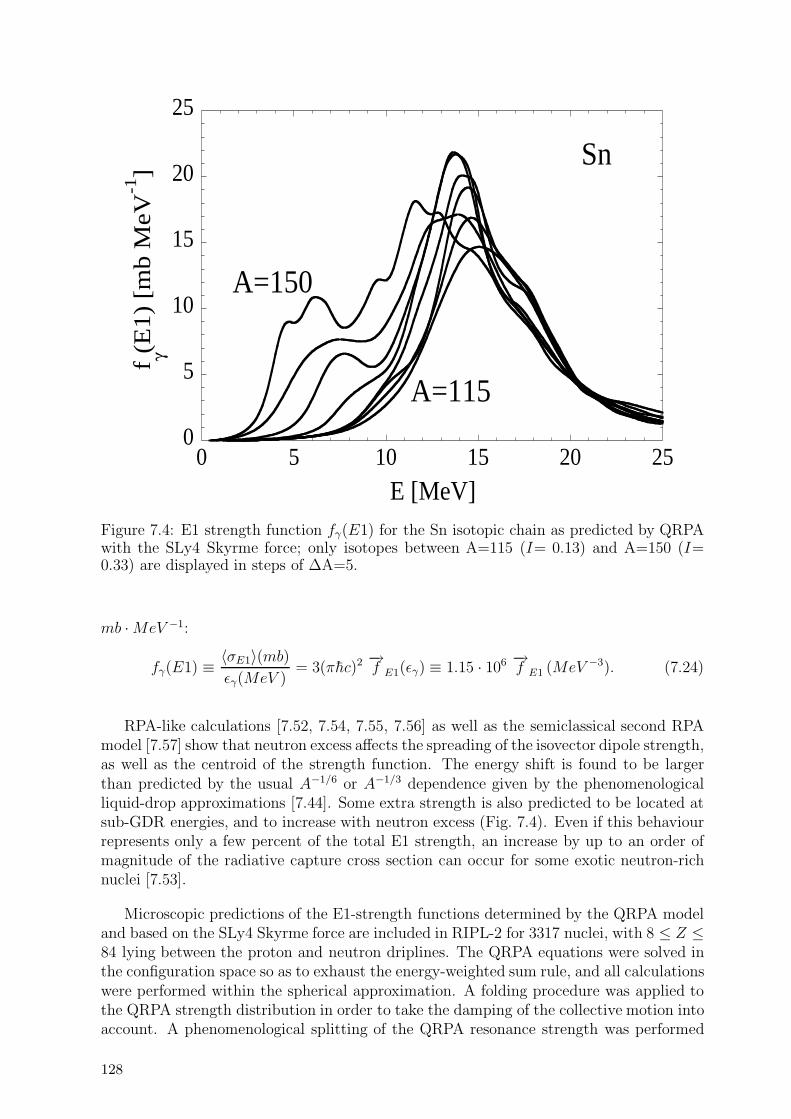
0

5

10

15

20

25

0 5 10 15 20 25

f γ(E1)

[mb M

eV-1

]

E [MeV]

Sn

A=115

A=150

Figure 7.4: E1 strength function fγ(E1) for the Sn isotopic chain as predicted by QRPAwith the SLy4 Skyrme force; only isotopes between A=115 (I= 0.13) and A=150 (I=0.33) are displayed in steps of ∆A=5.

mb ·MeV −1:

fγ(E1) ≡ 〈σE1〉(mb)

εγ(MeV )= 3(πhc)2 −→f E1(εγ) ≡ 1.15 · 106 −→f E1 (MeV −3). (7.24)

RPA-like calculations [7.52, 7.54, 7.55, 7.56] as well as the semiclassical second RPAmodel [7.57] show that neutron excess affects the spreading of the isovector dipole strength,as well as the centroid of the strength function. The energy shift is found to be largerthan predicted by the usual A−1/6 or A−1/3 dependence given by the phenomenologicalliquid-drop approximations [7.44]. Some extra strength is also predicted to be located atsub-GDR energies, and to increase with neutron excess (Fig. 7.4). Even if this behaviourrepresents only a few percent of the total E1 strength, an increase by up to an order ofmagnitude of the radiative capture cross section can occur for some exotic neutron-richnuclei [7.53].

Microscopic predictions of the E1-strength functions determined by the QRPA modeland based on the SLy4 Skyrme force are included in RIPL-2 for 3317 nuclei, with 8 ≤ Z ≤84 lying between the proton and neutron driplines. The QRPA equations were solved inthe configuration space so as to exhaust the energy-weighted sum rule, and all calculationswere performed within the spherical approximation. A folding procedure was applied tothe QRPA strength distribution in order to take the damping of the collective motion intoaccount. A phenomenological splitting of the QRPA resonance strength was performed

128

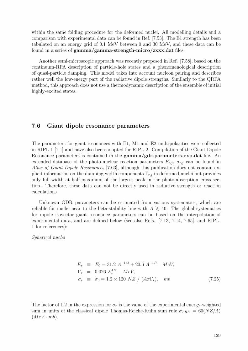
within the same folding procedure for the deformed nuclei. All modelling details and acomparison with experimental data can be found in Ref. [7.53]. The E1 strength has beentabulated on an energy grid of 0.1 MeV between 0 and 30 MeV, and these data can befound in a series of gamma/gamma-strength-micro/zxxx.dat files.

Another semi-microscopic approach was recently proposed in Ref. [7.58], based on thecontinuum-RPA description of particle-hole states and a phenomenological descriptionof quasi-particle damping. This model takes into account nucleon pairing and describesrather well the low-energy part of the radiative dipole strengths. Similarly to the QRPAmethod, this approach does not use a thermodynamic description of the ensemble of initialhighly-excited states.

7.6 Giant dipole resonance parameters

The parameters for giant resonances with E1, M1 and E2 multipolarities were collectedin RIPL-1 [7.1] and have also been adopted for RIPL-2. Compilation of the Giant DipoleResonance parameters is contained in the gamma/gdr-parameters-exp.dat file. Anextended database of the photo-nuclear reaction parameters Er,j, σr,j can be found inAtlas of Giant Dipole Resonances [7.63], although this publication does not contain ex-plicit information on the damping width components Γr,j in deformed nuclei but providesonly full-width at half-maximum of the largest peak in the photo-absorption cross sec-tion. Therefore, these data can not be directly used in radiative strength or reactioncalculations.

Unknown GDR parameters can be estimated from various systematics, which arereliable for nuclei near to the beta-stability line with A >∼ 40. The global systematicsfor dipole isovector giant resonance parameters can be based on the interpolation ofexperimental data, and are defined below (see also Refs. [7.13, 7.14, 7.65], and RIPL-1 for references):

Spherical nuclei

Er ≡ E0 = 31.2 A−1/3 + 20.6 A−1/6 MeV,

Γr = 0.026 E1.91r MeV,

σr ≡ σ0 = 1.2× 120 NZ / (AπΓr), mb (7.25)

The factor of 1.2 in the expression for σr is the value of the experimental energy-weightedsum in units of the classical dipole Thomas-Reiche-Kuhn sum rule σTRK = 60(NZ/A)(MeV ·mb).

129

Deformed nuclei

Er,1 = Er,2/[0.911

a0

b0+ 0.089

], Er,2 = E0

1

b0

[1− 1.51 · 10−2 · (a2

0 − b20)],

Γr,1 = 0.026E1.91r,1 , Γr,2 = 0.026E1.91

r,2 ,

σr,1 = σ0/3, σr,2 = 2σ0/3, (7.26)

where indexes 1 and 2 correspond respectively to the collective motion along and perpen-dicular to the axis of symmetry with relative semi-axes of a spheroid a0 = (1 + α2) /λ,b0 = (1− 0.5α2) /λ (see Eqs. 7.20 and 7.22).

The energy expressions in Eq. 7.26 were derived from the hydrodynamic model ofSteinwedel-Jensen [7.64] (Fig. 2 and Eq. 9), and for small deformations Er,1 � E0/(1+α2)and Er,2 � E0/(1 − 0.5α2) as reported in RIPL-12 [7.1]. Effective quadrupole deforma-tion parameters α2 or β2 of the equivalent spheroid (Eq. 7.20) were determined from the

ground-state deformation parameters βn ≡ αn

√(2n + 1)/4π, with the nuclear radius ex-

pansion expressed in spherical harmonics. βn parameters were calculated in Ref. [7.66],and are listed in the masses/mass-frdm95.dat file. The nuclear quadrupole moment Q

′

was calculated in units of (3/4π)ZeR20 for every nucleus by the equation (see also Eqs.1.22

and 6.19 in Ref. [7.67]):

Q′= α2 +

4

7α2

2 −1

7α3

2 −94

231α4

2 +8

7α2α4 +

72

77α2

2α4 +200

693α2

4, (7.27)

where αn ≡ βn/√

(2n + 1)/4π, with the ground-state deformation parameters βn taken

from Ref. [7.66]. The quadrupole deformation α2 of an effective spheroidal nucleus wasthen determined from the calculated quadrupole moment Q

′by solving the equation:

α2 +4

7α2

2 −1

7α3

2 −94

231α4

2 = Q′, (7.28)

where only terms up to the fourth order in α2 from the general expression for Q′

areretained. Effective quadrupole deformation parameters α2 have been determined this wayfor 8979 nuclei in the masses/mass-frdm95.dat file, and are tabulated in the deflib.datfile contained in the gamma/gamma-strength-analytic.tgz archive.

Nuclei at high excitation energy and with high angular momentum can be created inheavy-ion reactions. Static deformation is damped with increasing excitation energy, andthe nuclei become spherical. On the other hand, rotation leads to dynamic deformation,and calculation of the γ emission in such cases should use a spheroidal shape approxi-mation [7.8, 7.9, 7.68, 7.69]. Simple expressions were proposed in Ref. [7.70], based onthe liquid-drop model [7.71] with a rigid-body estimate for the nuclear moment of inertiaand a dynamic quadrupole deformation parameter for the rotating nuclei as a functionof angular momentum and mass number A. The oblate nucleus at slow rotation transits

2β was used in RIPL-1 instead of α2.

130

sharply to prolate shape when the frequency increases. General expressions are of theform:

β2 = β2 (I, A) = ES (I) (a1 + a2ES (I)) / (1 + a3ES (I))2

(7.29)

with

ai = bi + ci (A + di)2 , (7.30)

where ES (I) = E0rotI (I + 1) = 34.5A−5/3I (I + 1) MeV is the rotation energy of the

equivalent spherical nucleus with spin I . Slowly rotating spheroidal nuclei have an oblateshape, which changes to prolate shape at a critical angular momentum Icr. Coefficients bi,ci and di in Eq. 7.30 have the following values in the case of oblate nuclei (slow rotation):

b1 = −7.46 · 10−3, c1 = −1.94 · 10−7, d1 = −107.1;b2 = −4.20 · 10−5, c2 = −4.25 · 10−9, d2 = −93.90;b3 = 5.70 · 10−3, c3 = 2.44 · 10−7, d3 = −73.51.

(7.31)

Coefficients bi, ci and di for prolate nuclei (fast rotation) are:

b1 = −6.36 · 10−3, c1 = −6.33 · 10−7, d1 = −48.3;b2 = 1.02 · 10−3, c2 = 1.42 · 10−7, d2 = −95.9;b3 = 0.02, c3 = 8.59 · 10−7, d3 = −74.1.

(7.32)

The dependence of the critical spin Icr on mass number A and proton number Z is givenby the formula:

Icr = Icr (A, Z) = q1 + q2Z2 , (7.33)

where

qi = qi,1 + qi,2 · A + qi,3 · A2 , (7.34)

and

q1,1 = 55.10, q1,2 = − 0.063, q1,3 = 5.120 · 10−3;q2,1 = −0.013, q2,2 = 2.840 · 10−6, q2,3 = −2.570 · 10−7.

(7.35)

The dynamical deformation parameter at slow rotation (Eqs. 7.29 - 7.31) is practicallyidentical to the value obtained analytically in Refs. [7.46, 7.69, 7.72]:

β2 � −√

5π/4× 2.1A−7/3I(I + 1)/(1− 0.0205Z2/A). (7.36)

Macroscopic models describing the the relative motion of protons against neutronshave also been successful in reproducing experimental GDR energies and widths [7.44,

131

7.79]. An effect often neglected by systematics concerns the experimentally-observed shell-dependence of the GDR width, that can be explained by considering the coupling betweendipole oscillations and quadrupole surface vibrations [7.77]. RIPL-2 provides improvedpredictions of the GDR energies and widths for about 6000 nuclei from 14 ≤ Z ≤ 110lying between the proton and the neutron driplines. GDR is represented in the Goldhaber-Teller model [7.78], where the proton sphere vibrates against the neutron sphere. Thedynamics of the oscillation is assumed to be dominated by the np-interaction as describedin Ref. [7.79], with a renormalized strength K = 1360A−1/6 MeV fm3 derived froma least-squares fit to the experimental GDR energies [7.50]. Both the nucleon densitydistribution and ground-state deformation are taken from the Extended Thomas-Fermiplus Strutinsky Integral (ETFSI) compilation [7.80, 7.81]. The expression for the shell-dependent GDR width is taken from Ref. [7.77] using the newly-determined GDR energiesand the ETFSI shell corrections. Comparisons between predicted and experimental GDRenergies and widths are shown in Fig. 7.5; more details can be found in Ref. [7.50].GDR in deformed nuclei splitinto two peaks for oscillations parallel and perpendicularto the axis of rotational symmetry. All GDR energies and widths are tabulated in thegamma/gdr-parameters-theor.dat file.

7.7 M1 and E2 transitions

The GFL and MLO models can also be used to estimate the M1 strength←−f M1(εγ) over

a broad range of γ-ray energies when either experimental data or systematics for theratio R =

←−f E1(Bn)/

←−f M1(Bn) at neutron binding energy Bn are known. Then, the M1

strength function can be calculated from the following relationship:

←−f M1(εγ) =

←−f E1(Bn)

RφM1(εγ)

φM1(Bn), (7.37)

where φM1(εγ) describes the shape of the dipole magnetic radiative strength function,

and the dipole electric radiative strength←−f E1(Bn) is calculated using one of the models

discussed. Experimental values of the ratio R can be extracted for some nuclei fromthe gamma/gamma-strength-exp.dat file. Global parameterization of the R is givenby [7.1]:

R =

←−f E1(Bn)←−f M1(Bn)

= 0.0588 · A0.878, Bn ≈ 7 MeV. (7.38)

Two models are in common use for the function φM1:

(i) φM1(εγ) = const according to the single-particle model, and

(ii) φM1(εγ) from the SLO model (Eq. 7.4) and corresponding to the spin-flip giant res-onance mode [7.46], with the following global parameterization for the energy anddamping width [7.1]:

Er = 41 · A−1/3 MeV , Γr = 4 MeV .

132

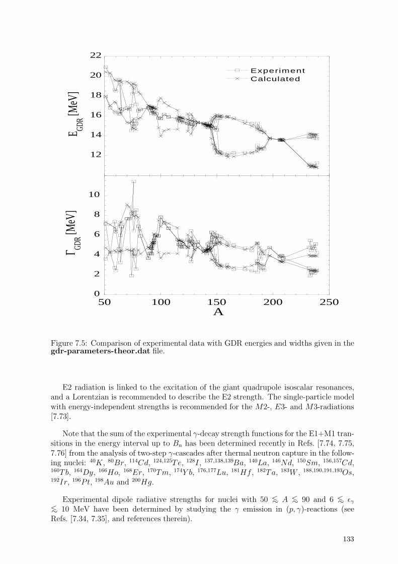
12

14

16

18

20

22

ExperimentCalculated

E GDR [M

eV]

0

2

4

6

8

10

50 100 150 200 250

Γ GDR [M

eV]

A

Figure 7.5: Comparison of experimental data with GDR energies and widths given in thegdr-parameters-theor.dat file.

E2 radiation is linked to the excitation of the giant quadrupole isoscalar resonances,and a Lorentzian is recommended to describe the E2 strength. The single-particle modelwith energy-independent strengths is recommended for the M2-, E3- and M3-radiations[7.73].

Note that the sum of the experimental γ-decay strength functions for the E1+M1 tran-sitions in the energy interval up to Bn has been determined recently in Refs. [7.74, 7.75,7.76] from the analysis of two-step γ-cascades after thermal neutron capture in the follow-ing nuclei: 40K, 80Br, 114Cd, 124,125Te, 128I , 137,138,139Ba, 140La, 146Nd, 150Sm, 156,157Cd,160T b, 164Dy, 166Ho, 168Er, 170Tm, 174Y b, 176,177Lu, 181Hf , 182Ta, 183W , 188,190,191,193Os,192Ir, 196Pt, 198Au and 200Hg.

Experimental dipole radiative strengths for nuclei with 50 <∼ A <∼ 90 and 6 <∼ εγ

<∼ 10 MeV have been determined by studying the γ emission in (p, γ)-reactions (seeRefs. [7.34, 7.35], and references therein).

133


Numerical studies indicate that the calculations of the γ-decay strength functions withinthe EGLO, GFL and MLO models give similar results at low γ-ray energies (εγ

<∼ 3 MeV ).These three models describe the experimental data much better than the SLO model atthese low energies, and also define a non-zero and temperature-dependent limit for thevanishing γ-ray energy. Results from the GFL, MLO and SLO models at εγ

>∼ 5 MeV arecloser to the experimental data than those obtained from EGLO. The E1 photo-excitationstrength functions for cold nuclei calculated with the MLO and SLO model agree over areasonably large range of γ-ray energies around the GDR peak.

The overall comparison between the EGLO, GFL, MLO and SLO models and experi-mental data showed that MLO and GFL provide the most reliable methods for determin-ing the E1 γ-ray strength functions over a relatively wide energy interval ranging fromzero to above the GDR peak. GFL and MLO are not time consuming calculational routesand are recommended for general use; both of them can be used to predict the statisticaldipole γ-ray emission and extract the GDR parameters from the experimental data forheated nuclei. We note that the GFL model is not consistent with the detailed balanceprinciple in systems with constant temperature, and the collisional components of theGFL damping width can become negative in some deformed nuclei.

A code has been developed as part of the RIPL-2 project to predict E1 strengthfunctions by means of the MLO, GFL, EGLO and SLO models, and is included in thegamma/gamma-strength-analytic.tgz file.

Large-scale QRPA calculations of the E1 strength have been undertaken in Ref. [7.53],and are tabulated in the gamma/gamma-strength-micro/zxxx.dat files that givethe same degree of accuracy as the MLO model in the energy range from 4 to 8 MeVfor nuclei close to the stability line. However, QRPA calculations reveal broadening ofthe GDR shape when moving away from the stability line. This effect stems from themicroscopic treatment and can not be accounted for by using experimental GDR shapes,which were measured for stable nuclei only. Thus, the use of the QRPA results can alsobe recommended for calculations on nuclei far from the stability line.



gamma-strength-analytic.readme - description of FORTRAN code for analytical cal-culation of the E1 strength function in terms of SLO, EGLO, MLO and GFL models.

gamma-strength-analytic.tgz - source of FORTRAN code for analytical calculationof the E1 strength function in terms of SLO, EGLO, MLO and GFL models.

gamma-strength-exp.dat - compilations of experimental E1 and M1 strength func-tions.

gamma-strength-exp.readme - description of gamma-strength-exp.dat file.

134

gamma-strength-micro/ - E1 strength functions determined within QRPA model.

gamma-strength-micro.readme - description of gamma-strength-micro file.

gdr-parameters-exp.dat - compilation of experimental giant dipole resonance param-eters.

gdr-parameters-exp.readme - description of gdr-parameters-exp.dat file.

gdr-parameters-theor.dat - theoretical predictions of the giant dipole resonance ener-gies and widths for about 6000 nuclei.

gdr-parameters-theor.readme - description of gdr-parameters-theor.dat file.

REFERENCES

[7.1] KOPECKY, J., “Gamma-Ray Strength Functions”, Handbook for calculationsof nuclear reaction data - Reference input parameter library, IAEA-TECDOC-1034, Vienna (1998) 97; directory GAMMA on the Web site http://www-nds.iaea.org/ripl/.

[7.2] BARTHOLOMEW, G.A., EARLE, E.D., FERGUSSON, A.J., KNOWLES, J.W.,LONE, M.A., Adv. Nucl. Phys. 7 (1973) 229.

[7.3] LONE, M.A., “Neutron induced reactions”, Proc. 4th. Int. Symp., Smolenice,Czechoslovakia, 1985, KRISTIAK, J., BETAK, E., REIDEL, D., (Eds.), Publ.Comp. Dordrecht, Holland (1986) 238.

[7.4] MONTOYA, C.P., SCHADMAND, S., DIOSZEGI, I., HOFMAN, D.J., ZHANG,P.H., PAUL, P., Z. Phys. A340 (1991) 371.

[7.5] SCHADMAND, S., VARMA, R., BANERJEE, S.R., BACK, B.B., HOFMAN,D.J., MONTOYA, C.P., PAUL, P., J. Phys. G21 (1995) 821.

[7.6] SNOVER, K., Ann. Rev. Nucl. Part. Sci. 36(1) (1986) 545.

[7.7] GAARDHOJE, J.J., Ann. Rev. Nucl. Part. Sci. 42 (1992) 483.

[7.8] BROGLIA, R.A., BORTIGNON, P.F., BRACCO, A., Prog. Part. Nucl. Phys. 28(1992) 517.

[7.9] PIERROUTSAKOU, D., AUGER, F., ALAMANOS, N., GOMES, P.R.S., SIDA,J.L., GILLIBERT, A., FRASCARIA, N., LHENRY, I., ROYNETTE, J.C.,SUOMIJARVI, T., Nucl. Phys. A600 (1996) 131.

[7.10] MATTIUZZI, M., BRACO, A. CAMERA, F., ORMAND, W.E., GAARDHØJE,J.J., MAJ, A., MILLION, B., PIGNANELLI, M., TVETER, T., Nucl. Phys.A612 (1997) 262.

[7.11] BRINK, D.M., PhD Thesis, University of Oxford (1955) 101.

[7.12] AXEL, P., Phys. Rev. 126 (1962) 671.

[7.13] BERMAN, B.L., FULTZ, S.C., Rev. Mod. Phys. 47 (1975) 713.

[7.14] DIETRICH, S.S., BERMAN, B.L., At. Data Nucl. Data Tables 38 (1988) 199.

135

[7.15] POPOV, Yu.P., “Neutron induced reactions”, Proc. Europhys. Topical Conf.,Smolenice, 1982, Physics and Applications, Vol. 10, OBLOZINSKY, P. (Ed.)(1982) 121.

[7.16] MCCULLAGH, C.M., STELTS, M., CHRIEN, R.E., Phys. Rev. C23 (1981) 1394.

[7.17] KOPECKY, J., UHL, M., Phys. Rev. C41 (1990) 1941.

[7.18] BECVAR, F., CEJNAR, P., CHRIEN, R.E., KOPECKY, J., Phys. Rev. C46(1992) 1276.

[7.19] COCEVA, C., Nuovo Cim. 107A (1994) 85.

[7.20] KADMENSKIJ, S.G., MARKUSHEV, V.P., FURMAN, V.I., Yad. Fiz. 37 (1983)277; Sov. J. Nucl. Phys. 37 (1983) 165.

[7.21] KOPECKY, J., UHL, M., CHRIEN, R.E., Phys. Rev. C47 (1993) 312.

[7.22] RING, P., ROBLEDO, L.M., EGIDO, J.L., FABER, M., Nucl. Phys. A419 (1984)261.

[7.23] EGIDO, J.L., WEIDENMUELLER, H., Phys.Rev. C39 (1989) 2398.

[7.24] EGIDO, J.L., RING, P., J. Phys. G19(1) (1993) 1.

[7.25] SPETH, J., VAN DE WOUDE, A., Rep. Prog. Phys. 44 (1981) 719.

[7.26] BERTSCH, G.F., BROGLIA, R.A., Oscillations in Finite Quantum Systems,Cambridge University Press, New York (1994).

[7.27] PLUJKO, V.A., Yad. Fiz. 52 (1990) 1004; Sov. J. Nucl. Phys. 52 (1990) 639.

[7.28] PLUJKO, V.A., Nucl. Phys. A649 (1999) 209c.

[7.29] PLUJKO, V.A., Acta Phys. Pol. B31 (2000) 435.

[7.30] PLUJKO, V.A., in Proc. 9th Int. Conf. Nucl. Reaction Mechanisms, Varenna,Italy, June 2000, GADIOLI, E. (Ed.) Suppl. N. 115 (2000) 113.

[7.31] PLUJKO, V.A., EZHOV, S.N., KAVATSYUK, M.O., GREBENUYK, A.A.,YERMOLENKO, R.V., in Proc. Int. Conf. Nuclear Data for Science and Technol-ogy, Oct. 2001, Tsukuba, Ibaraki, Japan. J. Nucl. Sci. Technol., Supp. 2 (August2002) 811.

[7.32] MUGHAGHAB, S.F., DUNFORD, C.L., Phys. Lett. B487 (2000) 155.

[7.33] SIROTKIN, V.K., Yad. Fiz. 43 (1986) 570.

[7.34] NEMSHKALO, B.A., SIROTKIN, V.K., SHEBEKO, K.B., Yad. Fiz. 55 (1992)123.

[7.35] FEDORETS, I.D., Yad. Fiz. 64 (2001) 51.

[7.36] EISENBERG, J.M., GREINER, W., Nuclear Theory, Vol. 1, Nuclear Models,Collective and Single-Particle Phenomena, North-Holland, Amsterdam (1987)Chapter 14, 3-5.

[7.37] DOVER, C.B., LEMMER, R.H., HAHNE, F.J.W., Ann. Phys. 70 (1972) 458.

[7.38] KOLOMIETZ, V.M., PLUJKO, V.A., SHLOMO, S., Phys. Rev. C54 (1996) 3014.

[7.39] PLUJKO, V.A., Acta Phys. Pol. B30 (1999) 1383.

136

[7.40] PLUJKO, V.A., GORBACHENKO, O.M., KAVATSYUK, M.O., Acta Phys.Slov. 51 (2001) 231; PLUJKO, V.A., EZHOV, S.N., GORBACHENKO, O.M.,KAVATSYUK, M.O., J. Phys.: Condensed Matter 14 (2002) 9473.

[7.41] OBLOZINSKY, P., Phys. Phys. C35 (1987) 407.

[7.42] BONASERA, A., BURGIO, G.F., DI TORO, M., Phys. Lett. B221 (1989) 233.

[7.43] SMERZI, A., BONASERA, A., DI TORO, M., Phys. Rev. C44 (1991) R1713.

[7.44] MYERS, W.D., SWIATECKI, W.J., KODAMA, T., EL-JAICK, L.J., HILF,E.R., Phys. Rev. C15 (1977) 2032.

[7.45] RAMAN, S., NESTOR, C.W., Jr., TIKKANEN, P., At. Data Nucl. Data Tables78 (2001) 1.

[7.46] BOHR, A.G., MOTTELSON, B.R., in Nuclear Structure, Vol. II, BenjaminLondon (1975) 636.

[7.47] LE TOURNEUX, J., Mat. Fys. Medd. Dan. Vid. Selsk. 34 (1965) 1.

[7.48] AYIK, S., BOILEY, D., Phys. Lett. B276 (1992) 263; ibid, B284 (1992) 482E.

[7.49] KOLOMIETZ, V.M., PLUJKO, V.A., SHLOMO, S., Phys. Rev. C52 (1995) 2480.

[7.50] GORIELY, S., Phys. Lett. B436 (1998) 10.

[7.51] GOVAERT, K., BAUWENS, F., BRYSSINCK, J., DE FRENNE, D., JACOBS,E., MONDELAERS, W., GOVOR, L., PONOMAREV, V.Yu., Phys. Rev. C57(1998) 2229.

[7.52] CATARA, F., LANZA, E.G., NAGARAJAN, M.A., VITTURI, A., Nucl. Phys.A624 (1997) 449.

[7.53] GORIELY, S., KHAN, E., Nucl. Phys. A706 (2002) 217.

[7.54] KHAN, E., SUOMIJARVI, T., BLUMENFELD, Y., NGUYEN VAN GIAI,ALAMANOS, N., AUGER, F., BAUGE, E., BEAUMEL, D., DELAROCHE,J.P., DELBOURGO-SALVADOR, P., DROUART, A., FORTIER, S., FRAS-CARIA, N., GILLIBERT, A., GIROD, M., JOUANNE, C., KEMPER, K.W.,LAGOYANNIS, A., LAPOUX, V., LEPINE-SZILY, A., LHENRY, I., LIBERT,J., MARECHAL, F., MAISON, J.M., MUSUMARRA, A., OTTINI-HUSTACHE,S., PIATTELLI, P., PITA, S., POLLACCO, E.C., ROUSSEL-CHOMAZ, P.,SANTONOCITO, D., SAUVESTRE, J.E., SCARPACI, J.A., ZERGUERRAS,T., Nucl. Phys. A694 (2001) 103.

[7.55] HAMOMOTO, I., SAGAWA, H., ZHANG, X.Z., Phys. Rev. C55 (1997) 2361;ibid, C57 (1998) R1064.

[7.56] VRETENAR, D., PAAR, N., RING, P., LALAZISIS, G.A., Nucl. Phys. A692(2001) 449.

[7.57] PLUJKO, V.A., KAVATSYUK, M.O., KAVATSYUK, O.O., Proc. 11th Int.Symp. Capture Gamma-Ray Spectr. and Related Topics (CGS 11), Pruhonicenear Prague, Czech Republic, Sept. 2002, KVASIL, J., CEJNAR, P., KRTICKA,M. (Eds.), World Scientific, Singapore (2003) 793.

[7.58] RODIN, V.A., URIN, M.G., Physics of Elementary Particle and Atomic Nuclei(Fyzika elementarnich chastitz i atomnogo yadra), Dubna, 31 (2000) 976.

137

[7.59] BUSH, B., ALHASSID, Y., Nucl. Phys. A531 (1991) 27.

[7.60] DILG, W., SCHANTL, W., VONACH, H., UHL, M., Nucl. Phys. A217 (1973) 269.

[7.61] VON EGIDY, T., SCHMIDT, H.H., BEHKAMI, A.N., Nucl. Phys. A481 (1988)189.

[7.62] SZEFLINSKI, Z., SZEFLINSKA, G., WILHELMI, Z., RZACA-URBAN, T.,KLAPDOR, H.V., ANDERSON, E., GROTZ, K., METZINGER, J., Phys. Lett.B126 (1983) 159.

[7.63] INTERNATIONAL ATOMIC ENERGY AGENCY, Handbook on photonucleardata for applications. Cross-sections and spectra. Final report of a co-ordinatedresearch project 1996-1999. IAEA-TECDOC-1178, Vienna (2000).

[7.64] DANOS, M., Nucl. Phys. 5 (1958) 23.

[7.65] CARLOS, P., BERGERE, R., BEIL, H., LEPRETRE, A., VEYSSIERE, A.,Nucl. Phys. A219 (1974) 61.

[7.66] MOLLER, P., NIX, J.R., MYERS, W.D., SWIATECKI, W.J., At. Nucl. DataTables 59 (1995) 185.

[7.67] HASSE, R.W., MYERS, W.D., Geometrical Relationships of Macroscopic NuclearPhysics, Springer-Verlag, Berlin, Heidelberg, New York (1988)

[7.68] BLANN, M., Phys. Rev. C21 (1980) 1770.

[7.69] BORTIGNON, P.F., BROGLIA, R.A., BRACCO, A., CASSING, W., DØSSING,T., ORMAND, W.E., Nucl.Phys. A495 (1989) 155c.

[7.70] GORBACHENKO, O.M., PLUJKO, V.A., Visnik Kyivskogo Universitetu, seriafis.-mat. nauk N1 (2001) 434; Abstracts 51th Conf. Nucl. Spectr. Nucl. Structure,September 2001, Sarov, Russia, VNIIEPH, P.130(304).

[7.71] BERINGER, R., KNOX, W.J., Phys. Rev. 121 (1961) 1195.

[7.72] VIGDOR, S.E., KARWOWSKI, H.J., Phys. Rev. C24 (1982) 1068.

[7.73] BLATT, M., WEISSKOPF, V.F., Theoretical Nuclear Physics, John Wiley, NewYork (1952) 647.

[7.74] VASILIEVA, E.V., SUKHOVOJ, A.M., KHITROV, V.A., Preprint P3-99-203,JINR, Dubna (1999).

[7.75] VASILIEVA, E.V., SUKHOVOJ, A.M., KHITROV, V.A., Physics of ElementaryParticle and Atomic Nuclei (Fyzika elementarnich chastitz i atomnogo yadra),Dubna, 31 (2000) 350.

[7.76] VASILIEVA, E.V., SUKHOVOJ, A.M., KHITROV, V.A., Yad. Fiz. 64 (2001) 3.

[7.77] THIELEMANN, F.K., ARNOULD, M., Proc. Conf. Nuclear Data for Science andTechnology, BOCKHOFF, K. (Ed.), Reidel, Dordrecht (1983) 762.

[7.78] GOLDHABER, M., TELLER, E., Phys. Rev. 74 (1948) 1046.

[7.79] VAN ISACKER, P., NAGARAJAN, M.A., WARNER, D.D., Phys. Rev. C45(1992) R13.

[7.80] GORIELY, S., in Proc. 10th Int. Symp. Capture Gamma-Ray Spectroscopy andRelated Topics, WENDER, S. (Ed.), AIP Conf. Proc. 529 (2002) 28.7

[7.81] ABOUSSIR, Y., PEARSON, J.M., DUTTA, A.K., TONDEUR, F., At. DataNucl. Data Tables 61 (1995) 127.

138

8 NUCLEAR FISSION

Coordinators: S. Goriely and A. Ignatyuk

Summary

A set of fission barriers and the corresponding nuclear level densities have been generatedfor various applications. Accurate level densities are prescribed within GSM for reactorphysics studies. Since fission level densities and barrier parameters are strongly interde-pendent, the corresponding set of parameters for both the inner and outer fission barriershas also been provided. Some specific applications, such as accelerator-driven systems andstellar nucleosynthesis, require a knowledge of large numbers of fission barriers and leveldensities to estimate spontaneous as well as neutron-induced or β-delayed fission prob-abilities. Hence, the present compilation includes fission barriers for some 2301 nucleiwith 78 ≤ Z ≤ 120 derived by means of the ETFSI method, and the corresponding leveldensities at both saddle-point deformations predicted by the microscopic model based onHFBCS single-particle properties.

The main concepts of nuclear fission theory are based essentially on the liquid-dropmodel [8.1, 8.2]. According to this model, competition between the surface tension forcesof a nuclear liquid drop and the Coulomb repulsion forces related to the nuclear chargeleads to the formation of an energy barrier which prevents spontaneous decay of the nu-cleus. The penetrability of the barrier determines the half-life for spontaneous fission. Inthe liquid-drop model, the height of the fission barrier for heavy nuclei decreases rapidlywith increase of Z2/A, and should disappear when (Z2/A)cr = 46− 48. The decrease inheight results in an exponential increase in barrier penetrability. These barrier changesexhibit good agreement with the behavior of the spontaneous fission lifetimes of the ac-tinide nuclei, ranging from the long-lived isotopes of uranium to the artificially synthesizedshort-lived isotopes of fermium and mendelevium [8.3, 8.4, 8.5, 8.6]. The height of thebarrier is a key ingredient for a description of fission cross sections measured in differentnuclear reactions.

Early studies show that despite some successful results the liquid-drop model can-not explain the major peculiarity of spontaneous and low-energy fission of the actinides,namely the asymmetric mass distribution of fission fragments [8.7], implying that shelleffects have a strong influence on fission fragment formation. Initially, fission mass-asymmetry was explained in terms of some modifications of the liquid-drop model pre-dictions for configurations close to the scission point (point where the fissioning nucleusbreaks into two fragments). However, new phenomena were discovered in the 1960s thatrequired more radical changes in the fission model in order to be explained, particularly

139

the spontaneously-fissioning Am isomers [8.8] and the intermediate resonance structuresobserved in the neutron-induced fission cross sections [8.9, 8.10] that cannot be explainedby adopting the traditional formula for fission barrier penetrability.

Calculations of nuclear deformation energies based on the shell correction method[8.11, 8.12] played a crucial role in explaining the above phenomena. The fission barrierscalculated for the actinides consisted of a two-hump curve with a rather deep potentialwell between the humps. This two-hump shape also identified the spontaneously-fissioningisomers as the lowest states of a fissioning nucleus in the second potential well, and theintermediate resonances as excited states of a nucleus in this well [8.13, 8.14].

Our present knowledge of the fission barriers can be represented in terms of threegroups:

(i) results of broad scale investigations of fission cross sections for pre-actinides thatundergo different charged-particle induced reactions to give the main experimentalinformation on the droplet properties of nuclei - interest in such data has increaseddramatically over the previous decade due to extensive discussions of accelerator-driven power systems for the transmutation of nuclear waste;

(ii) two-humped barriers of actinides studied with a high accuracy that undergo neutron-induced reactions of significant importance in reactor physics - investigations of thefission barriers at low energies were extended for many actinides to the high energiesof charged-particle induced reactions in order to study the changes of fission barrierswith increased excitation;

(iii) barriers required to explain the existence of long-lived superheavy elements with Z >102 due only to the shell effects in fission barriers - our knowledge and understandingof superheavy nuclei are still very scanty, and there are extremely large uncertaintiesassociated with the quantification of their fission barriers (see Ref. [8.15] for a goodreview of superheavy nuclei).

Our studies concentrate on the first two groups of data, which are connected withthe basic tasks of the RIPL project. Another field that requires extensive data on fissionbarriers is astrophysics which encompasses stellar nucleosynthesis and the rapid neutron-capture process. Microscopic calculations of the fission barriers associated with this phe-nomenon will be discussed in the final part of the chapter.

8.1 Fission barriers and level densities for pre-actinides

As with any other decay width, the fission width (Γf ) for an excited nucleus is deter-mined by the product of the excited level spacing (Dc) and the sum of the transmissioncoefficients over all channels leading to fission:

Γf (Uc) =Dc(Uc)

2π

∑Tfi . (8.1)

Based on the principles of the liquid-drop model, the intermediate saddle configuration atthe top of a fission barrier is of vital importance in the determination of fission probability.

140

A significant amount of the initial excitation energy at the saddle point is concentrated inthe fission degree of freedom, which imposes significant limitations on the excitations ofother degrees of freedom. Therefore, only the transitional states in the saddle point areusually considered as the fission channels [8.16]. The spectrum of such channels shouldbe similar to the observed level spectra of the heavy deformed nuclei, taking into accountpossible changes in the symmetry and deformation of transitional states. All limitationsconnected with the conservation laws for energy, angular momentum and parity shouldalso be taken into consideration in Eq. (8.1).

Most measurements of the fission cross sections for pre-actinides were performed atenergies above the fission barriers. Fission widths for such energies can be written in theform:

Γf (Uc) =1

2πρc(Uc)

Uc−Bf∫0

ρf(Uc − Bf −E)dE , (8.2)

where ρc and ρf are the level densities for the equilibrium compound and saddle configu-rations, respectively, and Bf is the fission barrier height [8.1]. Eq. (8.2) shows the stronginterdependence of the barrier parameters and the level densities. Approximations usedin the level density description of the fission cross-section analyses have been discussedby many authors [8.17, 8.18, 8.19, 8.20, 8.21], and the corresponding uncertainties of themodels applied should always be kept in mind when comparing the fission barriers derivedfrom available experimental data.

The most complete compilations of the experimental fission barriers are given in Refs.[8.22, 8.23, 8.24], where comprehensive sets of references can be found. A large amount ofdata has accumulated on the fission barriers for light charged-particle induced reactions.Many measurements of the fission cross sections were also performed for the heavy-ioninduced reactions [8.25]. However, because of the rather complex models involved inthe analysis of heavy-ion reactions, the uncertainties in the estimated fission barriers areusually found to be much larger than for light charged-particle reactions.

Generally, fission barriers are approximated by the equation:

Bf = Bld − δE0 + δEf , (8.3)

where Bld is the liquid-drop component of the fission barrier, δE0 is the ground state shellcorrection, and δEf is the corresponding shell correction for the saddle configuration ofthe fissioning nucleus. Usually, one assumes that the shell effects vanish for the strongly-deformed saddle configurations of pre-actinides, and the ground-state shell correctionsare equal to the microscopic corrections in the nuclear masses as considered in Chapter2. Differences between the various estimates of the fission barriers relate mainly to theliquid-drop component of the fission barrier.

Various versions of the liquid-drop model have been developed [8.26, 8.27, 8.28, 8.29],that differ as a consequence of the choice of model parameters and the additional compo-nents connected with the diffuse-surface, curvature and proximity effects. Rather simpleequations for the liquid-drop barriers were proposed recently on the basis of the Thomas-Fermi model [8.30]. Measured barriers for about 120 nuclei were fitted by the formula:

Bf (Z, N) = S(Z, N)F (X), (8.4)

141

where S = A2/3(1−kI2) is proportional to the nuclear surface energy with I = (N−Z)/A,and the surface symmetry coefficient k is defined as k = 1.9 + (Z − 80)/75. The fissionparameter (X) is proportional to the ratio of the Coulomb and surface energies, and canbe defined as

X = Z2/A(1− kI2). (8.5)

Function F is cubic, and joined smoothly to a straight line at X = X1:

F (X) =

{0.000199748(X0 −X)3 for X1 ≤ X ≤ X0,0.595553 − 0.124136(X −X1) for 30 ≤ X ≤ X1,

(8.6)

with X0 = 48.5428 and X1 = 34.15.

Available experimental data on the fission barriers for pre-actinides are comparedin Fig. 8.1 [8.23, 8.24] with the estimations derived from Eq. (8.4). The FRDM shellcorrections (see Chapter 2) were used to transform the experimental fission barriers toliquid-drop barriers. A good description of the experimental barriers led us to recommendEq. (8.4) as probably the best approximation of the liquid-drop fission barriers in theregion of X ≥ 30. Lighter nuclei have a dumb-bell shape at the saddle point, andthe calculations based on the Yukawa-plus-exponential double-folded approximation fornuclear energies may be preferable [8.29]. The corresponding code for such calculationsis included in RIPL-2, and the experimental fission barriers compiled in Ref. [8.24] fornear-magic nuclei with strong shell effects are given in the fission-barriers-exp.dat filetogether with the barriers for actinides (as discussed later). All models considered inChapter 6 can be used to calculate the fission widths (Eq. 8.1). However, in order tomaintain consistency, the same model should be used for the fission and particle widthsthat defined the dominant channels of a compound nucleus decay. The shell, pairingand collective effects are essentially different for the ground and saddle states, and thesedifferences should certainly be taken into account in calculations of nuclear fission.

Shell effects can apparently be neglected for the saddle level densities, but they areimportant for the neutron widths of near-magic nuclei shown in Fig. 8.1. The energydependence of the a-parameters given by Eqs. (6.11) and (6.36) is extremely important forsuch nuclei, as confirmed by many results of fission cross section analyses [8.20, 8.23, 8.31].

Pairing effects are implicitly associated with the energy dependence of the effectivemoment of inertia, which determines the angular distributions of the fission fragments[8.32]. Analysis of the corresponding experimental data has shown that the correlationparameter for the saddle point (∆f ) should always be specified as about 15% larger thanfor the ground states [8.33]. The relationship ∆f = 14/A1/2 can be used as a reasonableapproximation for the pairing parameter within the saddle point.

Collective enhancement of nuclear level densities is clearly displayed when undertakinga systematic analysis of the fission cross sections for spherical and deformed nuclei [8.19,8.21, 8.34]. A consistent description of the shell, pairing and collective effects can only beachieved by means of the generalized superfluid model (GSFM). GSFM parameters canbe derived on the basis of the systematics considered in Chapter 6, with correspondingmodifications to the pairing, asymptotic level density parameters and moments of inertiaof the saddle states.

Differences between the asymptotic level density parameters for the fission and neutronchannels are affected by the surface component for the density of single-particle states.

142

29 30 31 32 33 34

10

15

20

25

30

RePb

Ta

LuW

Ir

Os Pt Au Hg

At

Tl

Bi

Po

Bf (

MeV

)

Z2/A

Bexp

Bexp

-dE0

BMS

Figure 8.1: Fission barriers of pre-actinides and their liquid-drop components in compar-ison with liquid-drop model estimates [8.30]

Adopting the semi-classical approach, the level density parameter can be expressed in theform [8.20, 8.35, 8.36]

a = cvA + csBsA2/3 + ccBcA

1/3, (8.7)

where ci are the coefficients for the volume, surface and curvature components, and Bi arethe corresponding functions that describe the relative increase of the surface or curvatureunder deformation of a nucleus. The dumb-bell saddle shapes of pre-actinides correspondto Bs = 21/3, which leads to the ratio af/an > 1 used in all analyses of fission crosssections. However, there are large uncertainties associated with estimates of the coefficientratio cs/cv [8.20, 8.35, 8.36]. Evaluations of the ratio cs/cv = 1.30 based on microscopiccalculations involving the single-particle level schemes of the Wood-Saxon potential [8.20],or cs/cv = 1.53 derived from phenomenological systematics of the neutron resonancedensities seem to be the most reasonable approaches. Both methods give an af/an ratioof between 1.05 and 1.07 which is supported by the direct results of fission cross sectionanalyses [8.23].

8.2 Fission barriers and level densities for actinides

Highly accurate evaluations are required for the neutron-induced fission cross sections ofthe main fissile and fertile nuclei. The fission barriers and corresponding level densitiesare key ingredients of such evaluations. Full-scale Hauser-Feshbach theory, the coupled-

143

channel optical model and double-humped fission barrier parameterization are normallyused in such calculations, supported by numerous experimental data that demonstratethe importance of the shell, pairing and collective effects at both the equilibrium andsaddle nuclear states.

Eq. (8.1) is adopted for the fission width, but the transmission coefficients shouldbe estimated in accordance with the two-humped structure of fission barriers for whichpenetrabilities vary with energy in a much more complicated manner than for a one-humpbarrier [8.13, 8.14]. The quasi-stationary states of the nucleus in the well between thehumps have a strong modulating effect on the penetrability of the two-humped barrier[8.13, 8.37]. These modulations are manifested in the sub-barrier fission cross-sections asintermediate structures, examples of which are the resonances observed in the 230Th(n,f) reaction at neutron energies of about 700 keV [8.9] and the structure displayed in theneutron-induced fission cross-sections of 240Pu [8.10]. More comprehensive discussions ofthe experimental data on intermediate structures in actinide fission cross sections can befound in Refs. [8.13, 8.38].

The transmission coefficient for the deep second well can be averaged over the inter-mediate structures, and written in the form:

< T (E) >=TATB

TA + TB + Tγ(8.8)

where TA and TB are the penetrability of the humps A and B respectively, and Tγ is theprobability for gamma decay in the second well. The transition through the two-humpedbarrier is determined by the probability of sequential transitions through each of thehumps. If Tγ << (TA + TB), the probability of the transition through the asymmetrictwo-hump barrier is the same as that for the one-hump barrier and equivalent to thehigher hump.

Penetrabilities for each hump can be approximated by the well-known formula for thepenetrability of a parabolic barrier:

Ti(E) ={1 + exp

[2π

ωi

(Ei − E)]}−1

, (8.9)

where Ei is the energy of the transition state and ωi is the curvature close to the top ofthe corresponding barrier. As a consequence of the exponential growth of penetrability(which is much stronger than the decrease in level spacing), the average fission width (Eq.8.1) for the two-humped barrier increases exponentially with increasing excitation energyin an approximately similar manner to one higher hump. At energies above that of thebarrier, the penetrability does not prevent nuclear transitions to open fission channels,and the fission width increases because of the growth in the number of open channels,which is much weaker than the sub-barrier increase of the fission width. This change inthe growth rate of fission widths is usually adopted in experimental data analyses as adirect method for the estimation of fission barrier heights.

The quantum structure of the fission channels at the top of each barrier is extremelyimportant in the formulation of accurate descriptions of the fission cross sections at thesub-barrier and near-barrier energies. Such structure depends strongly on the symmetryof nuclear deformations at the corresponding saddle states. Shell model calculations

144

have been undertaken, supported by the results of fission fragment angular distributionanalyses. The fissioning nucleus has been calculated to possess axial asymmetric shape atthe inner saddle A, and axial-symmetric and mirror-asymmetric shape at the outer saddleB. Mirror-asymmetric even-even nuclei have ground-state rotational band levels withKπ = 0+, J = 0, 2, 4... - that unify with the octupole band levels Kπ = 0−, J = 1, 3, 5...in the common rotational band (which includes levels with all possible values of angularmomentum and parity). Additional unification arises for axial asymmetric shapes andlevels of the γ-vibrational band with Kπ = 2+, J = 2, 4... The quantum number ofthe corresponding rotational bands for odd and odd-odd nuclei should be estimated inaccordance with the angular momentum addition rules for unpaired particles and thecorresponding rotational bands. As the result, the fission cross section analysis involves amuch more complex structure of saddle transient states than the well-studied collective-level sequences of the deformed rare-earth nuclei and actinides.

The saddle shape symmetry should be taken into consideration when evaluating thecollective enhancement of the level densities. Thus, for axial-symmetric, mirror-asymmetricshapes, the rotational enhancement must be increased by a factor of two relative to theestimates given in Chapter 6 (Eq. 6.28). The rotational enhancement must be even largerfor γ-asymmetric shapes:

Krot = 2√

2π {IxIyIz}1/2 t3/2, (8.10)

where Ii is the moment of inertia relative to the corresponding axis, and t is the nu-clear temperature for transient states. Obviously, the moment of inertia should also becalculated for deformations corresponding to the saddle states.

The pairing effects at transient states are displayed most clearly in the energy de-pendence of the parameter K2

0 , which determines the angular distribution of the fissionfragments [8.32]. This parameter is proportional to the effective moment of inertia oftransient states, and is similar to the spin cutoff parameter in the level density formula(Eq. 6.1). The correlation function (∆f ) obtained from the analysis of the fission frag-ment angular distributions for even-even plutonium isotopes can be approximated by therelationship ∆f = 14/A1/2 MeV [8.39], and such an estimation of the pairing for thesaddle states is very close to the results obtained for the pre-actinides [8.33].

As a consequence of the essential role of the shell, pairing and collective effects, aconsistent description of the experimental data for the fission cross sections of actinidescan be obtained through the generalized superfluid model (GSFM). Data for the lightcharged-particle induced reactions have been analyzed for a large group of nuclei in Ref.[8.40] and for neutron-induced reactions in Refs. [8.41, 8.42, 8.43]. The neutron crosssections have been measured to a high degree of accuracy, and therefore their analyses areusually considered as the most reliable estimates of the fission barriers and fission leveldensities. Shell corrections were derived (in MeV) from an analysis of the fission crosssections in the first plateau region (2 - 5 MeV over the fission barrier) [8.41], using thephenomenological version of GSFM (see Chapter 6):

δEA0 =

{2.6 for Z ≤ 97,2.6− 0.1(Z − 97) for Z > 97,

δEB0 =

{0.6 + 0.1(Z − 97) + 0.04(N − 143) for Z < 97,0.6 + 0.04(N − 143) for Z ≥ 97

(8.11)

145

Pairing parameters were assigned ∆Af = ∆B

f = ∆0 + 0.2 MeV, where ∆0 is the pairingfor the ground states (neutron channels). The perpendicular moments of inertia for thelevel density calculations were chosen to be equal to 100h2/MeV for the inner saddle,200h2/MeV for the outer saddle, and approximately 75h2/MeV for the ground states[8.42].

Note that the matching of the discrete saddle states with the level density parametersused at high energies can be important for the consistent description of the fission crosssections at the near-barrier energies. Thus, the GSFM parameters for the fission channelsshould be estimated by adopting schemes for the saddle states of each hump; frequently,the constant temperature model is applied instead of adjusting such parameters. Thetemperatures are usually taken to be the same as for the neutron channels (see Chapter6), and the energy shifts are only adjusted to the adopted saddle state schemes.

Another important effect at the near-barrier energies is the step-like behavior of thelevel density near the thresholds of one- and two-quasi-particle excitations. Such step-like structures are observed directly in the low-energy variations of the parameter K2

0

determined from the fission fragment angular distribution [8.39], and can be explainedwithin the framework of GSFM [8.44]. The well-known structure in the neutron-inducedfission cross sections of 235U around 1 MeV can be considered as evidence of step-likechanges of the fission level density at the two-quasi-particle excitation threshold [8.42].An analysis of the irregularities in the neutron-induced fission cross sections of other nucleiis presented in Ref. [8.45]; the partial level density formula considered in Chapter 6 canbe applied to such irregularities, and possible simplifications were discussed.

Fission barrier parameters have been estimated from modeling analyses of the avail-able experimental data for the neutron-induced fission cross sections of the uranium,neptunium, plutonium, americium and curium isotopes [8.43, 8.46, 8.47]. Barrier pa-rameters for Th and Pa nuclei were also obtained by adopting essentially the same ap-proach [8.48, 8.49, 8.50]; however, these specific data were less accurately estimated dueto the more complex structure of the fission barriers in light actinides as compared totransuranium nuclei. The inner and outer fission barrier heights are shown in Fig. 8.2.Corresponding data were included in the RIPL-1 files, and have been combined with therecommended barriers for pre-actinides in the fisbar-experimental.dat file of RIPL-2. A comparison between these data and the fission barriers evaluated in Ref. [8.24]shows that there is good agreement for the outer barriers of the uranium, plutonium andamericium isotopes. Some disagreements exist for the inner barrier heights, although thegeneral isotopic dependences are very similar; furthermore, significant discrepancies occurin the case of the outer barriers of the curium isotopes.

Barrier curvature parameters are usually evaluated with relatively large uncertaintiesfrom analyses of the sub-barrier behavior of fission cross sections [8.38, 8.45]. The followingparameters can be recommended as optimal (in MeV): hA = 0.9− 1.0, 0.8 and 0.60, andhB = 0.6, 0.5 and 0.4 for the even-even, odd and odd-odd nuclei, respectively. Even-odddifferences in the curvature parameters are dependent on the superconductive pairingcorrelations and their impact on the stiffness and reduced mass parameters of the fissioningnucleus at the saddle.

Pairing parameters for the fission channels are given in the recommended data files,together with the corresponding fission barriers. These data are shown in Fig. 8.3 in com-

146

225 230 235 240 245 250

5

6

7

8

Am

Np

Pu

Cm

Pa

U

ThAt

Ra

Mass number

BB (

MeV

)

4

5

6

7 Am

Cm

Pu

Np

U

Pa

Th

BA (

MeV

)

Figure 8.2: Inner (A) and outer (B) fission barriers derived from the analysis of neutron-induced fission cross sections [8.46, 8.47, 8.48, 8.49, 8.50].

parison with the simple approximations used in the systematics of the pairing parametersfor the equilibrium and saddle states. An increase of the pairing at the saddle point isconfirmed by all results of the fission cross section analysis, but the difference between∆f and ∆0 seems to fluctuate strongly. Variations of ∆f have an important effect on thefission barrier values extracted from the cross-section analysis. Despite such well-definedvariations, the uncertainties in the fission barrier parameters are difficultly to estimateaccurately. For even-even nuclei in which the sub-barrier and over-barrier cross sectionsare analyzed simultaneously, the uncertainties in the higher-hump estimates are about0.2 MeV; these uncertainties are even larger for the lower hump with values of about 0.5MeV. Approximately the same uncertainties should be adopted for the fission barriers ofodd and odd-odd nuclei for which the over-barrier cross sections can be analyzed. Finally,the uncertainties of the outer barriers of the curium isotopes are probably ever larger.

Many of the above results were obtained from analyses of the fission cross sections atexcitations lower than 15 - 20 MeV above the fission barrier. According to the generalconcepts of the shell correction method, the two-humped structure of any fission barriershould disappear at higher excitation, and liquid-drop fission barriers with asymptoticlevel density parameters should be used to describe both the fission cross section and

147

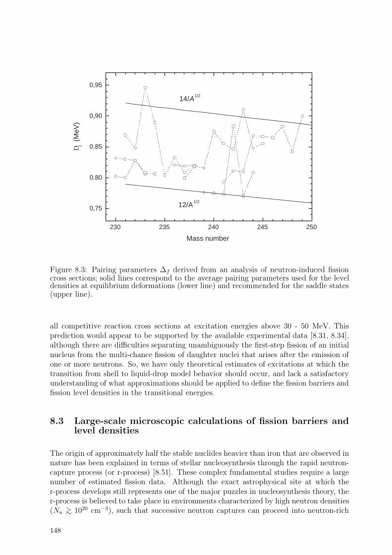
230 235 240 245 250

0,75

0,80

0,85

0,90

0,95

12/A1/2

14/A1/2

Df (

MeV

)

Mass number

Figure 8.3: Pairing parameters ∆f derived from an analysis of neutron-induced fissioncross sections; solid lines correspond to the average pairing parameters used for the leveldensities at equilibrium deformations (lower line) and recommended for the saddle states(upper line).

all competitive reaction cross sections at excitation energies above 30 - 50 MeV. Thisprediction would appear to be supported by the available experimental data [8.31, 8.34],although there are difficulties separating unambiguously the first-step fission of an initialnucleus from the multi-chance fission of daughter nuclei that arises after the emission ofone or more neutrons. So, we have only theoretical estimates of excitations at which thetransition from shell to liquid-drop model behavior should occur, and lack a satisfactoryunderstanding of what approximations should be applied to define the fission barriers andfission level densities in the transitional energies.

8.3 Large-scale microscopic calculations of fission barriers andlevel densities

The origin of approximately half the stable nuclides heavier than iron that are observed innature has been explained in terms of stellar nucleosynthesis through the rapid neutron-capture process (or r-process) [8.51]. These complex fundamental studies require a largenumber of estimated fission data. Although the exact astrophysical site at which ther-process develops still represents one of the major puzzles in nucleosynthesis theory, ther-process is believed to take place in environments characterized by high neutron densities(Nn >∼ 1020 cm−3), such that successive neutron captures can proceed into neutron-rich

148

regions some considerable distance from the valley of β-stability. This process producesnuclei with decreasing neutron binding energies, and consequently faster (γ, n) photodis-integration that competes with the slowing-down (n, γ) reactions at high temperatures(T >∼ 109 K). With timescales usually thought to be much longer than the characteristictimescale of (n, γ) and (γ, n) reactions, β-decay drives the material to higher Z elements.Depending on the strength of the neutron flux as well as the duration of the neutronirradiation, nuclei up to the super-heavy mass region can be produced in timescales ofthe order of a second. So far, no astrophysical model is able to provide any reliablepredictions of the thermodynamic conditions under which the r-process can take place.Fission processes are important in describing the nuclear mechanisms taking place duringthe r-process:

(i) if matter reaches the super-heavy neutron-rich region during the neutron irradiation,fission could recycle the nuclear flow and affect the nucleosynthesis of the bulk ofthe r-process nuclei;

(ii) all nuclei produced during the r-process irradiation with A >∼ 208 are neutron-richheavy progenitors of the r-abundance peak in the Pb region - their productionratio depends on the fission probabilities, so that a correct treatment of the fissionprocesses is needed to predict the production of Pb and Bi during and after neutronirradiation;

(iii) r-process nucleosynthesis creates long-lived 232Th, 235U and 238U that are used ascosmochronometers to estimate the upper age limit of the Galaxy [8.52].

An accurate knowledge of the astrophysics, as well as the nuclear properties affecting theprogenitors of these chronometers (particularly the fission probabilities of their progeni-tors) is a fundamental pre-requisite for a reliable age estimate.

Changes in the abundance of the heavy nuclei as a result of the high neutron fluxesand temperatures encountered during the r-process nucleosynthesis can only be satisfac-torily calculated by using a network of nuclear reactions that includes all of the necessaryneutron capture, photodisintegration, β-decay, α-decay, β-delayed particle and fission pro-cesses. The fission processes include spontaneous, β-delayed and neutron-induced fissionfor which the probabilities must be estimated for some 2000 nuclei with 80 <∼ Z <∼ 110 lo-cated mainly in the neutron-rich region. Therefore, we have compiled fission-barrier datafor some 2301 nuclei with 78 ≤ Z ≤ 120 as derived using the ETFSI method, and the cor-responding level densities at both saddle point deformations predicted by the microscopicmodel (more details are given below).

8.3.1 Fission barriers

Data file fisbar-etfsi.dat contains predictions of the fission barriers and saddle pointdeformations as obtained from the Extended Thomas-Fermi plus Strutinsky Integral(ETFSI) model [8.53, 8.54]. ETFSI is a semi-classical approximation to the Hartree-Fock method in which the shell corrections are calculated with the “integral” version ofthe Strutinsky theorem; BCS corrections are also added with a delta-pairing force. Thefission barriers are derived with the SkSC4 Skyrme force on which the ETFSI-1 mass

149

formula is based. Experimental primary barriers can be reproduced [8.24] within plus orminus 1.5 MeV (except for elements with Z < 87 which have barriers above 10 MeV).Fig. 8.4 shows the relative accuracy (Bexp−Bth)/Bexp of this global prediction for the pri-mary barriers, i.e., the highest barrier (see Ref. [8.53] for more details). These predictionsare accurate to within ± 40%, which is an excellent result in view of the global characterof the model based on a Skyrme force fitted exclusively in terms of nuclear masses.

-0.4

-0.2

0

0.2

0.4

190 200 210 220 230 240 250 260

InnerOuter

(Bex

p-Bth

)/B

exp

A

Figure 8.4: Relative errors (Bexp−Bth)/Bexp in the primary (i.e., highest) barriers calcu-lated by ETFSI.

The ETFSI compilation includes 2301 nuclei with 78 ≤ Z ≤ 120, and their massesrange from slightly neutron-deficient to extremely neutron-rich nuclei (close to or at thecalculated neutron drip line) up to A = 318. These data contain the nuclei considered inRef. [8.53] for which experimental barriers are known, and a slightly extended version ofthe set published in Ref. [8.54]. Experimental fission barriers are also included that werecompiled in Ref. [8.53] and originated mainly from Ref. [8.24].

A maximum of two barriers are given for each nucleus (inner and outer), correspondingto the highest saddle points among the “slightly” and “strongly” deformed. Those twogroups of saddle points correspond to well-separated values of the elongation parameter c(cin and cout (see below)); cin < 1.6 and cout > 1.6 for many nuclei, although 1.5 < cout <1.6 in some cases.

As well as the calculated inner and outer barriers, the deformation parameters at thecorresponding saddle points are included in the RIPL-2 database. The nuclear shapesare limited to axially symmetrical deformations that are described in terms of Brackparameterization (c, h, α), where c is the elongation parameter (c < 1, = 1 and > 1 foroblate, spherical and prolate shapes, respectively), h is associated with the “necking”of the nuclear surface (shapes corresponding to different regions of the (c, h) plane aredescribed in Ref. [8.53]), and α quantifies left-right asymmetry (α = 0 for symmetricshapes). Asymmetry parameters ain and aout listed in RIPL-2 do not refer to α, butto α as defined in Ref. [8.53] to be α c3; the mass ratio of the two fission fragments isroughly given by (1+3/8 α)/(1−3/8 α). All calculated fission barriers have deformationparameters within the domain: 1.00 < c < 2.36, −0.26 < h < 0.22 and 0 ≤ α < 0.75.

150

8.3.2 Fission level densities

Level densities need to be provided for all the nuclei of interest. As already stressed,shell, pairing and deformation effects are essential input in the provision of a reliableestimate of the level densities at the fission saddle points. Furthermore, the most appro-priate model that includes all these effects in a consistent form is the microscopic modelbased on the partition function method, as described in Chapter 6 [8.55]. This modelis based on HFBCS single-particle properties, and predicts all the experimental s-waveresonance spacings with accuracies comparable to those obtained by the phenomenologi-cal BSFG formula. HFBCS is characterized by a nucleon effective mass close to the realmass [8.56], which is a particularly important parameter for reliable evaluations of leveldensities (provides a good description of the single-particle level density near the Fermisurface). When extrapolating level densities to exotic neutron-rich super-heavy nuclei, amicroscopic approach might also be more stable than a phenomenological model.

The level density model includes:

• BCS pairing (in the constant-G approximation) with a renormalized strength andblocking effect for odd-mass and doubly-odd nuclei;

• Gaussian-type spin dependence, with microscopic shell and pairing effects that im-pact on the spin cut-off parameter;

• deformation effects that modify the single-particle spectra and the collective contri-bution of the rotational bands on top of each intrinsic state;

• an improved description at very-low energies [8.55].

The single-particle level scheme is consistently calculated for each saddle point bythe deformed HFBCS model, based on the MSk7 Skyrme force [8.56] and constrainedon the saddle-point quadrupole, octupole and hexadecapole moments. Identical pairingstrengths (within the constant-G approximation) are used in these calculations and todetermine the level density of the ground-state equilibrium deformation. However, noconsideration is given to the possibility of a damping of the collective effects at increasingexcitation energies.

The level densities are separately given the inner (levden-hfbcs-inner subdirectory)and outer (levden-hfbcs-outer subdirectory) saddle points as tabulations covering 2300nuclei, with 78 ≤ Z ≤ 120 included in the ETFSI compilation of fission barriers. Eachtable includes the spin-dependent level densities for energies up to U = 150 MeV and spinup to J = 29 (59/2). The nuclear temperature, cumulative number of levels, and totallevel and state densities are also included in the tables. Ground-state level densities areavailable in table format [8.55], and have been included in the RIPL-2 compilation (seeChapter 6). Note that the level density for left-right asymmetric fission barriers shouldbe increased by a factor of 2 (this correction is not included in the tables).

Predicted fission level densities can be quantified in terms of the af/a ratio (i.e., a-parameter at the saddle point (af) corresponding to the (inner or outer) fission barrierexpressed as a fraction of the equilibrium ground-state configuration (a)). Two examples

151

0.95

1.00

1.05

1.10

1.15

1.20

1.25

1.30

af/a intrinsic

af/a with rot. enh.

a f / a

232Th: Outer barrier β2=0.95; β

4=0.24

0.90

0.95

1.00

1.05

1.10

1.15

1.20

1.25

0 25 50 75 100 125 150

af/a intrinsic

af/a with rot. enh.

a f / a

U[MeV]

238U: Inner barrier β2=0.41; β

4=-0.03

Figure 8.5: af/a ratios with and without (i.e., intrinsic) rotational enhancement as afunction of the excitation energy for 232Th and 238U predicted by the HFBCS-based nuclearlevel density.

are shown in Fig. 8.5: two estimates of af/a ratio for 232Th outer and 238U inner barriers.Saddle-point deformations correspond to the values determined by the ETFSI model.First estimate corresponds to the intrinsic af/a ratio, i.e., entropy Sf/S ratio (a = U/t2

differs from a = S/2t in the microscopic approach, and consequently the entropy ratiomust be considered to estimate the traditional a-ratio used in practical applications).Second estimate gives the equivalent a-ratio when the rotational enhancement factor isimplicitly included in the a-parameter:

ρ(U) =

√π

12 a1/4 U5/4exp(2

√a U) (8.12)

where ρ(U) correspond to the general formula (Eq. 6.1) in which the total microscopiclevel density with the collective contribution of the rotational bands was adopted.

The level densities have not been extensively tested on fission cross sections. However,a preliminary analysis of neutron-induced fission at low energies shows that a system-atic increase of level densities is required to reproduce the experimental cross section

152

if use is made of the RIPL-2 recommended fission barriers (as given in the fisbar-experimental.dat file and described in the previous section). This increase can beobtained by a shift of approximately 1 MeV in the energy scale provided in the leveldensity tables.


Fission barriers and fission level densities are key ingredients of the statistical descriptionof the fission cross sections induced by different incident particles. The fission barrierparameters derived from analyses of the available experimental data have been compiledfor both pre-actinides and actinides. Two groups of fissioning nuclei can be formulatedthat differ essentially in their barrier properties:

(i) fission barriers close to the liquid-drop model predictions with the ground-state shellcorrections for the pre-actinides, and

(ii) two-humped barriers with strong shell effects in the ground-state, and both humpsfor actinides.

The fission density models used for nuclear data evaluations should include in a con-sistent manner all variations of the shell, pairing and collective effects related to thefission barrier structures. A phenomenological or microscopic version of the generalizedsuperfluid model appears to be the most suitable for such tasks, coupled with significantchanges to the level density parameters of the fission channels as recommended above.

The RIPL-2 files include a large amount of data produced from microscopic calcula-tions of the fission barriers (based on the ETFSI) and fission level densities (based onthe HFBCS single-particle level schemes). The microscopic model takes into account theshell, pairing and blocking effects, the deformation effects in the single-particle spectra,and the collective enhancement of level densities at low excitation energies and their dis-appearance at high excitations. Corresponding tables of the level densities for about 2301nuclei with 87 ≤ Z ≤ 120 are provided in RIPL-2.


The structure of the corresponding RIPL-2 directory is as follows:

fission/fisbar-experimental.datfisbar-experimental.readmefisbar-etfsi.datfisbar-etfsi.readmefisbar-liquiddrop.forfisbar-liquiddrop.readmelevden-hfbcs.readmelevden-hfbcs-inner/Zxxx.datlevden-hfbcs-outer/Zxxx.dat

153

Programs and data files included in the directory are:

fisbar-experimental.dat - fission barrier parameters derived from the analysis of ex-perimental data available for pre-actinides and actinides.

fisbar-experimental.readme - description of fisbar-experimental.dat file.

fisbar-etfsi.dat - fission barriers for 2301 nuclei with 78 ≤ Z ≤ 120 calculated by meansof the Extended Thomas-Fermi plus Strutinsky Integral (ETFSI) method.

fisbar-etfsi.readme - description of fisbar-liquiddrop.for file.

fisbar-liquiddrop.for - FORTRAN code for the liquid-drop model calculations of thefission barriers and the moment of inertia of fissioning nuclei.

fisbar-liquiddrop.readme - description of fisbar-liquiddrop.for file.

levden-hfbcs.readme - description of levden-hfbcs-inner/Zxxx.dat andlevden-hfbcs-outer/Zxxx.dat files.

levden-hfbcs-inner/Zxxx.dat, levden-hfbcs-outer/Zxxx.dat - level densities cal-culated for the inner and outer fission barriers, respectively, based on the microscopicapproach HFBCS single-particle level schemes.

REFERENCES

[8.1] BOHR, N., WHEELER, J.A., Phys. Rev. 56 (1939) 426.

[8.2] FRENKEL, Ya.I., JETP 9 (1939) 641.

[8.3] GHIORSO, A., HARVEY, B.G., CHOPPIN, G.R., THOMPSON, S.G.,SEABORG, G.T., Phys. Rev. 98 (1955) 1518;GHIORSO, A., THOMPSON, S.G., HIGGINS, G.H., SEABORG, G.T.,STUDIER, M.H., FIELDS, P.R., FRIED, S.M., DIAMOND, H., MECH, J.F.,PYLE, G.L., HUIZENGA, J.R., HIRSCH, A., MANNING, W.M., BROWNE,C.I., SMITH, H.L., SPENCE, R.W., Phys. Rev. 99 (1955) 1048.

[8.4] FLEROV, G.N., 2nd Conf. Peaceful Uses of Atomic Energy, United Nations,Geneva, 14 (1958) 151.

[8.5] FLEROV, G.N., TER-AKOPIAN, G.M., Sov. Part. Nucl. 46 (1983) 817.

[8.6] SEABORG, G.T., LOVELAND, W.D., Elements beyond Uranium, Wiley, NewYork (1990).

[8.7] VANDENBOSH, R., HUIZENGA, J.R., Nuclear Fission, Academic Press, NewYork (1973).

[8.8] POLIKANOV, S.M., et al., JETP 42 (1962) 1464.

[8.9] VOROTNIKOV, P.E., DUBROVINA, S.M., OTROSHCHENKO, G.A., SHIGIN,V.A., Sov. J. Nucl. Phys. 5 (1967) 207.

[8.10] MIGNEKO, E., THEOBALD, J.P., Nucl. Phys. A112 (1968) 603.

154

[8.11] STRUTINSKY, V.M., Sov. J. Nucl. Phys. 3 (1966) 449; ibid., Nucl. Phys. A95(1967) 420.

[8.12] STRUTINSKY, V.M., Nucl. Phys. A122 (1968) 1.


[8.14] BJORNHOLN, S., STRUTINSKY, V.M., Nucl. Phys. A136 (1969) 1.

[8.15] HOFMANN, S., MUNZENBERG, G., Rev. Mod. Phys. 72 (2000) 733.

[8.16] BOHR, A., 1st Conf. Peaceful Uses of Atomic Energy, Geneva, 1955, UnitedNations, NY, 2 (1955) 151.

[8.17] THOMPSON, S.G., Arkiv Fysik 36 (1967) 267.

[8.18] MORETTO, L.G., Physics and Chemistry of Fission, IAEA, Vienna, Vol. 1 (1974)329.

[8.19] FREIESLEBEN, H., BRITT, H.C., HUZENGA, J.R., Physics and Chemistry ofFission, IAEA, Vienna, Vol. 1 (1974) 421.

[8.20] IGNATYUK, A.V., ITKIS, M.G., OKOLOVICH, V.N., SMIRENKIN, G.N.,TISHIN, A.S., Sov. J. Nucl. Phys. 21 (1976) 612.


[8.22] DAHLINGER, M., VERMEULEN, D., SCHMIDT, K.H., Nucl. Phys. A376(1982) 94.

[8.23] IGNATYUK, A.V., et al., Sov. Part. Nucl. 16 (1985) 709.

[8.24] SMIRENKIN, G.N., INDC(CCP)-359, IAEA, Vienna (1993).

[8.25] OGANESSIAN, Yu.Tc., LAZAREV, Yu.A., Treatise on Heavy-Ion Science,BROMLEY, D. (Ed.), Vol. 4 (1987) 3.

[8.26] COHEN, S., SWIATECKI, W.J., Ann. Phys. 22 (1963) 406.

[8.27] HASSE, R.W., Ann. Phys. 68 (1971) 377.

[8.28] KRAPPE, H.J., NIX, J.R., SIERK, A.J., Phys. Rev. C20 (1979) 992.

[8.29] SIERK, A.J., Phys. Rev. C33 (1986) 2039.

[8.30] MYERS, W.D., SWIATECKI, W.J., Phys. Rev. C60 (1999) 014606.

[8.31] VIGDOR, S.E., KARWOWSKI, H.J., JACOBS, W.W., KAILAS, S., SINGH,P.P., SOGA, F. THROWE, T.G., Phys. Rev. C26 (1982) 1035.

[8.32] HALPERN, I., STRUTINSKY, V.M., 2nd Conf. Peaceful Uses of Atomic Energy,United Nations, Geneva 15 (1958) 408.


[8.34] JUNGHANS, A.R., DE JONG, M., CLERC, H-G., IGNATYUK, A.V.,KUDYAEV, G.A., SCHMIDT, K-H., Nucl. Phys. A629 (1998) 635.

[8.35] TOKE, J., SWIATECKI, W.J., Nucl. Phys. A372 (1981) 141.

155

[8.36] REISDORF, W., Z. Phys. A300 (1981) 227.

[8.37] GAI, E.V., IGNATYUK, A.V., RABOTNOV, N.S., SMIRENKIN, G.N., Sov. J.Nucl. Phys. 10 (1970) 311.

[8.38] BJORNHOLN, S., LYNN, J.R., Rev. Mod. Phys. 52 (1980) 725.

[8.39] SHPAK, D.L., OSTAPENKO, Yu.B., SMIRENKIN, G.N., Sov. J. Nucl. Phys. 13(1971) 950.

[8.40] GAVRON, A., BRITT, H.C., KONECNY, E., WEBER, J., WILHELMY, J.B.,Phys. Rev. C13 (1976) 2374;GAVRON, A., BRITT, H.C., GOLDSTONE, P.D., SCHOENMACKERS, R.,WEBER, J., WILHELMY, J.B., Phys. Rev. C15 (1977) 2238.

[8.41] KUPRIYANOV, V.M., SMIRENKIN, G.N., FURSOV, B.I., Sov. J. Nucl. Phys.39 (1984) 281.

[8.42] IGNATYUK, A.V., MASLOV, V.M., Sov. J. Nucl. Phys. 54 (1991) 647.

[8.43] MASLOV, V.M., KIKUCHI, Y., Nucl. Sci. Eng. 124 (1996) 492.

[8.44] IGNATYUK, A.V., SOKOLOV, Yu.V., Sov. J. Nucl. Phys. 19 (1974) 1229.

[8.45] MASLOV, V.M., Z. Phys. A347 (1994) 211.

[8.46] MASLOV, V.M., SUKHOVITSKIJ, E.Sh., PORODZINSKIJ, Yu.V.,KLEPATSKIJ, A.B., MOROGOVSKIJ, G.B., INDC(BLR)-4, INDC(BLR)-5, IAEA, Vienna (1996).

[8.47] MASLOV, V.M., SUKHOVITSKIJ, E.Sh., PORODZINSKIJ, Yu.V., MOROGOV-SKIJ, G.B., INDC(BLR)-7, INDC(BLR)-9, INDC(BLR)-10, IAEA, Vienna (1997).

[8.48] MASLOV, V.M., Ann. Nucl. Energy 19 (1992) 181.

[8.49] MASLOV, V.M., Yadernye Konstanty 1 (1992) 80.

[8.50] MASLOV, V.M., Yadernye Konstanty 4 (1987) 19.

[8.51] ARNOULD, M., TAKAHASHI, K., Rep. Prog. Phys. 62 (1999) 393.

[8.52] GORIELY, S., ARNOULD, M., Astron. Astrophys. 379 (2001) 1113.

[8.53] MAMDOUH, A., PEARSON, J.M., RAYET, M., TONDEUR, F., Nucl. Phys.A644 (1998) 389.

[8.54] MAMDOUH, A., PEARSON, J.M., RAYET, M., TONDEUR, F., Nucl. Phys.A679 (2001) 337.

[8.55] DEMETRIOU, P., GORIELY, S., Nucl. Phys. A695 (2001) 95.

[8.56] GORIELY, S., TONDEUR, F., PEARSON, J.M., At. Data Nucl. Data Tables 77(2001) 311.

156

ERRATA

The RIPL potentials 9101 (Huizenga Igo), 9401(Nolte) and 9600(Avrigeanu) for alpha-induced reactions were corrected in the RIPL-2 database on 10 September 2004. Theirimaginary part was defined as a surface potential, when it should be volume potential.

157

List of participants

T. Belgya: Institute of Isotope and Surface Chemistry Chemical Research Centre,Budapest, Hungary

O. Bersillon: Centre d’Etudes Nucleaires de Bruyeres-le-Chatel, France

R. Capote Noy: Centro de Estudios Aplicados al Desarrollo Nuclear, Havana, Cuba

T. Fukahori: Japan Atomic Energy Tokai-mura, Naka-gun, Japan

Ge Zhigang: China Institute of Atomic Energy, Beijing, China

S. Goriely: Universite Libre de Bruxelles, Brussels, Belgium

M. Herman: Scientific Secretary (from March 2000),

International Atomic Energy Agency

A.V. Ignatyuk: Institute of Physics and Power Engineering, Obninsk,

Russian Federation

S. Kailas: Bhabha Atomic Research Centre, Bombay, India

A.J. Koning: Nuclear Research and Consultanc Group, Petten, Netherlands

P. Oblozinsky: Brookhaven National Laboratory, Upton, USA (Scientific Secretaryuntil March 2000, International Atomic Energy Agency)

V. Plujko: Taras Shevchenko National University, Kiev, Ukraine

P.G. Young: Chairman, Los Alamos National Laboratory, Los Alamos, USA

159

,

,

y

Agency

r

handbook for calculations of nuclear reaction data, ripl-2 · pdf filehandbook for...

Documents