ieee transactions on signal ... - systems.caltech.edu

IEEE TRANSACTIONS ON SIGNAL PROCESSING, VOL. 55, NO. 8, AUGUST 2007 4139

Quadratically Constrained Beamforming RobustAgainst Direction-of-Arrival Mismatch

Chun-Yang Chen, Student Member, IEEE, and P. P. Vaidyanathan, Fellow, IEEE

Abstract—It is well known that the performance of the min-imum variance distortionless response (MVDR) beamformer isvery sensitive to steering vector mismatch. Such mismatches canoccur as a result of direction-of-arrival (DOA) errors, local scat-tering, near-far spatial signature mismatch, waveform distortion,source spreading, imperfectly calibrated arrays and distorted an-tenna shape. In this paper, an adaptive beamformer that is robustagainst the DOA mismatch is proposed. This method imposes twoquadratic constraints such that the magnitude responses of twosteering vectors exceed unity. Then, a diagonal loading methodis used to force the magnitude responses at the arrival anglesbetween these two steering vectors to exceed unity. Therefore, thismethod can always force the gains at a desired range of anglesto exceed a constant level while suppressing the interferencesand noise. A closed-form solution to the proposed minimizationproblem is introduced, and the diagonal loading factor can becomputed systematically by a proposed algorithm. Numericalexamples show that this method has excellent signal-to-interfer-ence-plus-noise ratio performance and a complexity comparableto the standard MVDR beamformer.

Index Terms—Capon beamformer, diagonal loading, direc-tion-of-arrival (DOA) mismatch, minimum variance distortionlessresponse (MVDR) beamformer, robust beamforming, steeringvector uncertainty.

I. INTRODUCTION

BEAMFORMING has long been used in many areas, suchas radar, sonar, seismology, medical imaging, speech

processing, and wireless communications. An introduction tobeamforming can be found in [25]–[30] and the referencestherein.

A data-dependent beamformer was proposed by Caponin [1]. By exploiting the second-order statistics of the arrayoutput, the method constrains the response of the signal ofinterest (SOI) to be unity and minimizes the variance of thebeamformer output. This method is called minimum variancedistortionless response (MVDR) beamformer in the literature.The MVDR beamformer has very good resolution, and thesignal-to-interference-plus-noise ratio (SINR) performance ismuch better than traditional data-independent beamformers.However, when the steering vector of the SOI is imprecise, theresponse of the SOI is no longer constrained to be unity and isthus attenuated by the MVDR beamformer while minimizing

Manuscript received March 29, 2006; revised October 22, 2006. This workwas supported in part by the ONR under Grant N00014-06-1-0011 and in partby The California Institute of Technology. The associate editor coordinating thereview of this manuscript and approving it for publication was Dr. A. RahimLeyman.

The authors are with the California Institute of Technology (Caltech),Pasadena, CA 91125 USA (e-mail: [email protected]).

Digital Object Identifier 10.1109/TSP.2007.894402

the total variance of the beamformer output [2]. The effect iscalled signal cancellation. It dramatically degrades the outputSINR. Many approaches, including [6]–[24] and the referencestherein, have been proposed for improving the robustness of theMVDR beamformer. A good introduction to this topic can befound in [3]. The steering vector of the SOI can be imprecisebecause of various reasons, such as direction-of-arrival (DOA)errors, local scattering, near-far spatial signature mismatch,waveform distortion, source spreading, imperfectly calibratedarrays, and distorted antenna shape [3], [4]. In this paper, wefocus on DOA uncertainty.

There are many methods developed for solving the DOA mis-match problem. In [13]–[20], linear constraints have been im-posed when minimizing the output variance. The linear con-straints can be designed to broaden the main beam of the beam-pattern. These beamformers are called linearly constrained min-imum variance (LCMV) beamformers. In [22] and [23], convexquadratic constraints have been used. In [21], a Bayesian ap-proach has been used. For other types of mismatches, diagonalloading [11], [12] is known to provide robustness. However, thedrawback of the diagonal loading method is that it is not clearhow to choose a diagonal loading factor. In [24], the steeringvector has been projected onto the signal-plus-interference sub-space to reduce the mismatch. In [5], the magnitude responsesof the steering vectors in a polyhedron set are constrained to ex-ceed unity while the output variance is minimized. This methodavoids the signal cancellation when the actual steering vector isin the designed polyhedron set. In [6], Vorobyov et al. have useda nonconvex constraint which forces the magnitude responsesof the steering vectors in a sphere set to exceed unity. This non-convex optimization problem has been reformulated in a convexform as a second-order cone programming (SOCP) problem.It has been also proven in [6] that this beamformer belongs tothe family of diagonal loading beamformers. In [7] and [8], thesphere uncertainty set has been generalized to an ellipsoid setand the SOCP has been avoided by the proposed algorithmswhich efficiently calculate the corresponding diagonal loadinglevel. In [9], a general rank case has been considered using asimilar idea as in [6] and an elegant closed-form solution hasbeen obtained.

In [5]–[9], the magnitude responses of steering vectors in anuncertainty set have been forced to exceed unity while mini-mizing the output variance. The uncertainty set has been se-lected as polyhedron, sphere, or ellipsoid in order to be ro-bust against general types of steering vector mismatches. Inthis paper, we consider only the DOA mismatch. Inspired bythese uncertainty-based methods, we consider a simplified un-certainty set which contains only the steering vectors with a

1053-587X/$25.00 © 2007 IEEE

4140 IEEE TRANSACTIONS ON SIGNAL PROCESSING, VOL. 55, NO. 8, AUGUST 2007

desired uncertainty range of DOA. To find a suboptimal so-lution for this problem, the constraint is first loosened to twononconvex quadratic constraints such that the magnitude re-sponses of two steering vectors exceed unity. Then, a diag-onal loading method is used to force the magnitude responsesat the arrival angles between these two steering vectors to ex-ceed unity. Therefore, this method can always force the gains ata desired range of angles to exceed a constant level while sup-pressing the interference and noise. A closed-form solution tothe proposed minimization problem is introduced, and the di-agonal loading factor can be computed systematically by a pro-posed iterative algorithm. Numerical examples show that thismethod has excellent SINR performance and a complexity com-parable to the standard MVDR beamformer.

The rest of this paper is organized as follows: The MVDRbeamformer and the analysis of steering vector mismatch arepresented in Section II. Some previous work on robust beam-forming is reviewed in Section III. In Section IV, we developthe theory and the algorithm of our new robust beamformer.Numerical examples are presented in Section V. Finally, con-clusions are presented in Section VI.

Notations: Boldfaced lowercase letters such as representvectors, and boldfaced uppercase letters, such as , denotematrices. The element in row and column of matrixis denoted by . The notation denotes the conjugatetranspose of the vector . Notation denotes the expectationof the random variable .

II. MVDR BEAMFORMER AND THE

STEERING VECTOR MISMATCH

Consider a uniform linear array (ULA) of omnidirectionalsensors with interelement spacing . The SOI is a narrowbandplane wave impinging from angle . The baseband array output

can be expressed as

where denotes the sum of the interferences and the noises,is the SOI, and represents the baseband array response

of the SOI. It is called the “steering vector” and can be expressedas

(1)

where is the operating wavelength. The output of the beam-former can be expressed as , where is the complexweighting vector. The output signal-to-interferences-plus-noiseratio (SINR) of the beamformer is defined as

(2)

where , and . By varyingthe weighting factors, the output SINR can be maximized byminimizing the total output variance while constraining the SOI

response to be unity. This can be written as the following opti-mization problem:

subject to (3)

where This is equivalent to minimizingsubject to because

The solution to this problem is well known and was first givenby Capon in [1] as

(4)

This beamformer is called the MVDR beamformer in the litera-ture. When there is a mismatch between the actual arrival angle

and the assumed arrival angle , this beamformer becomes

(5)

It can be viewed as the solution to the minimization problem

subject to (6)

Since , andis no longer valid due to the mismatch, the SOI magnitude

response might be attenuated as a part of the objective function.This suppression leads to severe degradation in SINR, becausethe SOI is treated as interference in this case. The phenomenonis called “signal cancellation.” A small mismatch can lead tosevere degradation in the SINR.

III. PREVIOUS WORK ON ROBUST BEAMFORMING

Many approaches have been proposed for improving the ro-bustness of the standard MVDR beamformer. In this section, webriefly mention some of them related to our work.

A. Diagonal Loading Method

In [11] and [12], the optimization problem in (3) is modifiedas

subject to

This approach is called diagonal loading in the literature. It in-creases the variance of the artificial white noise by the amount

. This modification forces the beamformer to put more effortin suppressing white noise rather than interference. As before,

CHEN AND VAIDYANATHAN: QUADRATICALLY CONSTRAINED BEAMFORMING 4141

when the SOI steering vector is mismatched, the SOI is atten-uated as one type of interference. As the beamformer puts lesseffort in suppressing the interferences and noise, the signal can-cellation problem addressed in Section II is reduced. However,when is too large, the beamformer fails to suppress stronginterference because it puts most effort to suppress the whitenoise. Hence, there is a tradeoff between reducing signal cancel-lation and effectively suppressing interference. For that reason,it is not clear how to choose a good diagonal loading factor inthe traditional MVDR beamformer.

B. LCMV Method

In [13]–[20], the linear constraint of the MVDR in (3) hasbeen generalized to a set of linear constraints as

subject to (7)

where is an matrix and is an vector. The solu-tion can be found by using the Lagrange multiplication methodas

This is called the LCMV beamformer. These linear constraintscan be directional constraints [15], [16] or derivative constraints[17]–[19]. The directional constraints force the responses ofmultiple neighbor steering vectors to be unity. The derivativeconstraints not only force the response to be unity but also sev-eral orders of the derivatives of the beampattern in the assumedDOA to be zero. These constraints broaden the main beam ofthe beampattern so that it is more robust against the DOA mis-match. In [20], linear constraints have further been used to allowan arbitrary specification of the quiescent response.

C. Extended Diagonal Loading Method

In [6], the following optimization problem is considered:

subject to (8)

where is a sphere defined as

(9)

where is the assumed steering vector. The constraint forces themagnitude responses of an uncertainty set of steering vectors toexceed unity. The constraint is actually nonconvex. However,in [6], it is reformulated to a second-order cone programming(SOCP) problem which can be solved by using some existingtools, such as SeDuMi in MATLAB. It has also been provenin [6] that the solution to (8) has the form forsome appropriate and . Therefore, this method can be viewedas an extended diagonal loading method [7]. In [7] and [8], theuncertainty set in (9) has been generalized to an ellipsoid, and

the SOCP has been avoided by the proposed algorithms whichdirectly calculate the corresponding diagonal loading level asa function of , , and .

D. General-Rank Method

In [9], a general-rank signal model is considered. The steeringvector is assumed to be a random vector that has a covari-ance . The mismatch is therefore modeled as an error matrix

, in the signal covariance matrix , and an errormatrix in the output covariance matrix . Thefollowing optimization problem is considered:

subject to

where denotes the Frobenius norm of the matrix , andand are the upperbounds of the Frobenius norms of the error

matrices and , respectively. This optimization problemhas an elegant closed-form solution as shown by Shahbazpanahiet al. in [9], namely

(10)

where denotes the principal eigenvector of the matrix. The principal eigenvector is defined as the eigenvector cor-

responding to the largest eigenvalue.

IV. NEW ROBUST BEAMFORMER

In this paper, we consider the DOA mismatch. When there isa mismatch, the minimization in (6) suppresses the magnituderesponse of the SOI. To avoid this, we should force the magni-tude responses at a range of arrival angles to exceed unity whileminimizing the total output variance. This optimal robust beam-former problem can be expressed as

subject to (11)

where and are the lower and upperbounds of the uncer-tainty of SOI arrival angle, respectively, and is the steeringvector defined in (1) with the arrival angle . The following un-certainty set of steering vectors is considered:

(12)

where , and . This uncer-tainty set is a curve. This constraint protects the signals in therange of angles from being suppressed.

A. Frequency-Domain View of the Problem

Substituting (12) into the constraint in (11), the constraint canbe rewritten as


Fig. 1. Frequency-domain view of the optimization problem.

where is the Fourier transform of the weight vector. The objective function can also be rewritten in the

frequency domain as

where is the power spectral density (PSD) of the arrayoutput . Therefore, the optimization problem can be rewrittenin the frequency domain as

subject to for

Note that is a weighting function in the above integral.The frequency-domain view of this optimization problem is il-lustrated in Fig. 1. The integral of is mini-mized while for is satisfied. Eventhough we will not solve the problem in the frequency domain,it is insightful to look at it this way.

B. Two-Point Quadratic Constraint

It is not clear how to solve the optimal beamformer in(11) because the constraint does not fit into any of the existingstandard optimization methods. The constraintfor can be viewed as an infinite number ofnonconvex quadratic constraints. To find a suboptimal solution,we start looking for the solution by loosening the constraint.We first loosen the constraint by choosing only two constraints

and from the infinite con-

straints for . The correspondingoptimization problem can be written as

subject to and (13)

Due to the fact that the constraint is loosened, the minimum tothis problem is a lowerbound of the original problem in (11).Note that the constraint in (13) is a nonconvex quadratic con-straint. In order to obtain an analytic solution, we reformulatethe problem in the following equivalent form:

subject to

where

and , , and are real numbers.To solve this problem, we divide it into two parts. We first

assume , , and are constants and solve . The solutionwill be a function of , , and . Then, the solution

can be substituted back into the objective function so that theobjective function becomes a function of , , and . Finally,we minimize the new objective function by choosing , , and

. Define the function

(14)

where is the Lagrange multiplier. Taking the gradientof (14) and equating it to zero, we obtain the solution

Substituting the above equation into the constraint, the Lagrangemultiplier can be expressed as

Substituting back into , we obtain

(15)

Given , , and , can be found from the above equa-tion. Note that it is exactly the solution to the LCMV beam-former mentioned in Section III-B with two directional con-straints. Therefore, this approach can be viewed as an LCMVbeamformer with a further optimized in (7). However, this ap-proach is reformulated from the nonconvex quadratic problemin (13). It is intrinsically different from a linearly constrainedproblem. The task now is to solve for , , and . Write


where , , and are real non-negative numbers. Substitutingin (15) into the objective function, it becomes

(16)

To minimize the objective function, can be chosen as

(17)

so that the last equality in (16) holds. Now and are obtainedby (17) and (15), and the objective function becomes (16). Tofurther minimize the objective function, and can be foundby solving the following optimization problem:

This can be solved by using the Karush–Kuhn–Tucker (KKT)condition. The following solution can be obtained:

(18)

Summarizing (15), (17), and (18), the following algorithm forsolving the beamformer with the two-point quadratic constraintin (13) is obtained.

Algorithm 1

Given , , and , compute by the following steps:

The matrix inversion in Step 2 contains most of the com-plexity of the algorithm. Therefore, the algorithm has the sameorder of complexity as the MVDR beamformer. Since the con-straint is loosened, the feasible set of the two-point quadraticconstraint problem in (13) is a superset of the feasible set of theoriginal problem in (11). The minimum found in this problemis a lowerbound of the minimum of the original problem. If thesolution in the two-point quadratic constraint problem in

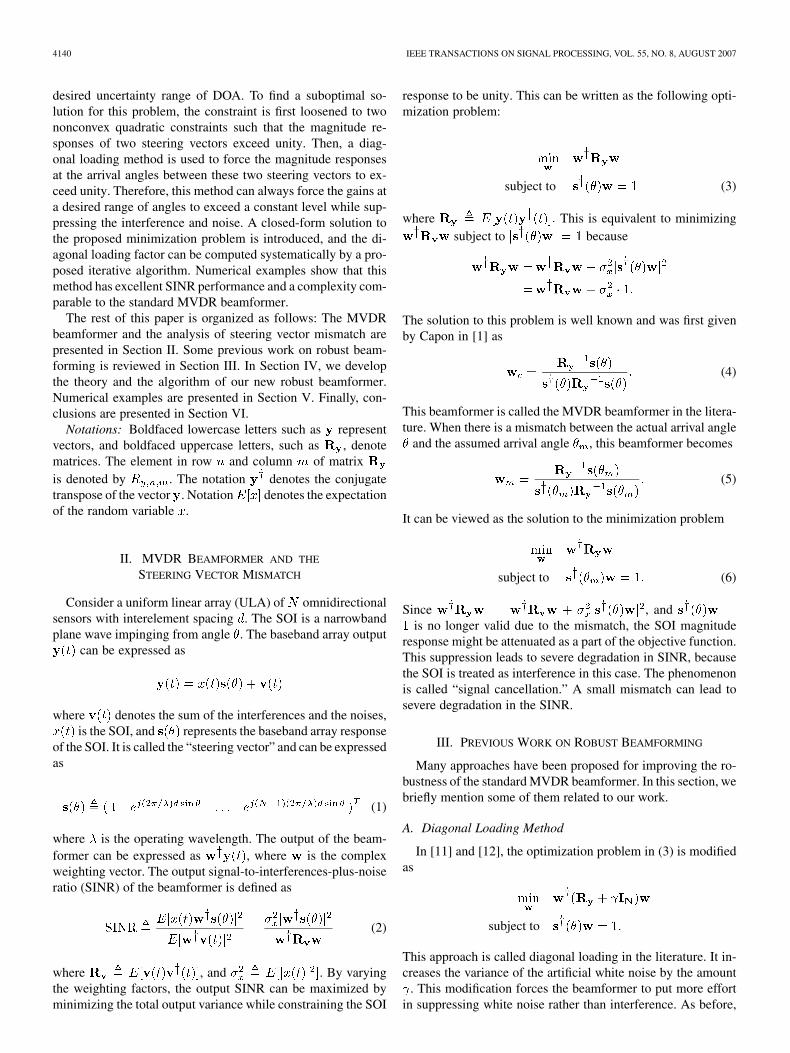
Fig. 2. Example of a solution of the two-point quadratic constraint problemthat does not satisfy jsywj � 1 for � � � � � .

(13) happens to satisfy the original constraintfor , then is exactly the solution to the orig-inal problem in (11). The example provided in Fig. 1 is actuallyfound by using the two-point quadratic constraint instead of theoriginal constraint, but it also satisfies the original constraint.This makes it exactly the solution to the original problem in (11).

Unfortunately, in general, the original constraintfor is not guaranteed to be satisfied by the

solution of the two-point quadratic constraint problem in (13).Fig. 2 shows an example where the original constraint is notsatisfied. This example is obtained by increasing the power ofthe SOI in the example in Fig. 1. One can comparein Figs. 1 and 2 and find that the SOI power is much stronger inFig. 2. In this case, the beamformer tends to put a zero between

and to suppress the strong SOI. This makesfor some between and . The original constraint is

thus not satisfied. This problem will be overcome by a methodprovided in Section V.

C. Two-Point Quadratic Constraint With Diagonal Loading

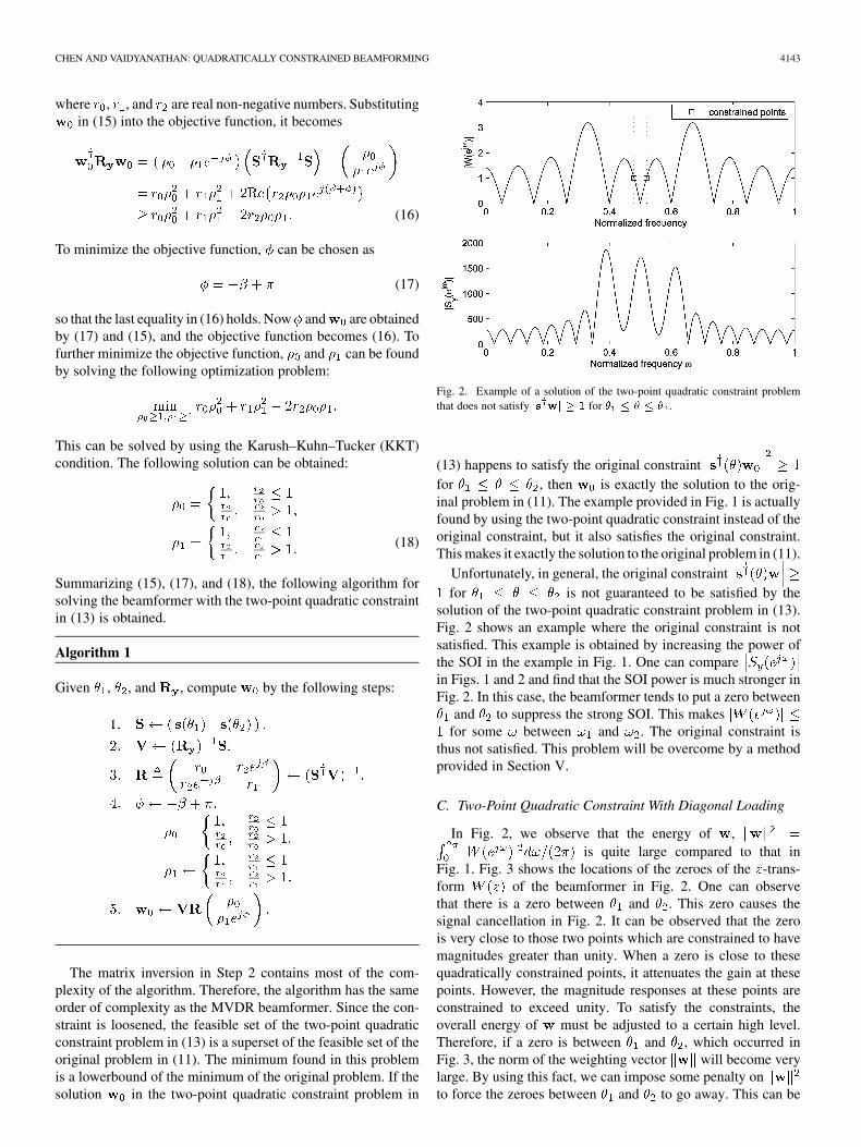
In Fig. 2, we observe that the energy of ,is quite large compared to that in

Fig. 1. Fig. 3 shows the locations of the zeroes of the -trans-form of the beamformer in Fig. 2. One can observethat there is a zero between and . This zero causes thesignal cancellation in Fig. 2. It can be observed that the zerois very close to those two points which are constrained to havemagnitudes greater than unity. When a zero is close to thesequadratically constrained points, it attenuates the gain at thesepoints. However, the magnitude responses at these points areconstrained to exceed unity. To satisfy the constraints, theoverall energy of must be adjusted to a certain high level.Therefore, if a zero is between and , which occurred inFig. 3, the norm of the weighting vector will become verylarge. By using this fact, we can impose some penalty onto force the zeroes between and to go away. This can be


Fig. 3. Locations of zeroes of the beamformer in Fig. 2.

accomplished by the diagonal loading approach mentioned inSection III-A. The corresponding optimization problem can bewritten as

subject to and (19)

where is the diagonal loading factor which represents theamount of the penalty put on . The solution can befound by performing the following modification on the outputcovariance matrix:

and then applying Algorithm 1. When , the solutionconverges to

subject to and (20)

The following lemma gives the condition for which satisfiesthe constraint for all in .

Lemma 1: for if and only if

Proof: According to (20), substituting and ap-plying Algorithm 1, one can obtain

sincd

where

and sincd

By direct substitution, one can obtain

sincd sincd

sincd(21)

where and

if sincdotherwise.

By (21), it can be verified that

if and only if

which can also be expressed asIf the condition is satisfied,

exists such that the condition foris satisfied. For example, if , , , and

, then we have

In this case, exists so that the robust conditionfor 35 is satisfied. However,

introducing the diagonal loading changes, the objective func-tion to . The modification of theobjective function affects the suppression of the interferences.To keep the objective function correct, should be chosenas small as possible while the condition for

is satisfied. For finding such a , we propose thefollowing algorithm.

Algorithm 2

Given , , , an initial value of , a search step size, and a set of angles , which satisfies

for all , can be computed by the followingsteps:

Compute by Algorithm 1

If for all

then stop.

else and go to 1.

Fig. 4 illustrates how Algorithm 2 works. In this figure, theset is the feasible set ofthe two-point quadratic constraint problem in (13). The set

is the feasible set of themismatched steering vector problem in (11). If the condition

is satisfied, Lemma 1 shows that. In this case, exists so that . Algorithm

2 keeps increasing by multiplying until


for all is satisfied. This is an approximation forThe number can be very small. In Section V,

works well for all of the cases. Also, the SINR is not sensitiveto the choice of , as we will see later.

V. NUMERICAL EXAMPLES

For the purpose of design examples, the same parametersused in [8] are used in this section. A uniform linear array (ULA)of omnidirectional sensors spaced a half-wavelengthapart (i.e., ) is considered. There are three signals im-pinging upon this array, as follows:

1) the SOI with an angle of arrival ;2) an interference signal with an angle of arrival

;3) another interference signal with an angle of arrival

.The received narrowband array output can be modeled as

where is the steering vector defined in (1), and is thenoise. We assume , , , and are the zero-mean wide-sense stationary random process satisfying

(40 dB above noise)

(20 dB above noise)

Thus, the covariance matrix of the narrowband array outputcan be expressed as

1) Example 1: SINR versus diagonal loading factor .In this example, the actual arrival angle is 43 , but the as-

sumed arrival angle is 45 . The SINR defined in (2) is com-pared for a different diagonal loading factor . The followingfive methods involving diagonal loading are considered:

1) Algorithm 1 in Section IV with the new method withand ;

2) general-rank method [9] in (10) with the parameter

3) diagonal loading method [11], [12] in Section III-A;4) directional LCMV [15], [16] with two linear constraints

which forces the responses of the signals from 42 and 48to be unity;

5) derivative LCMV [17]–[19] with two linear constraintswhich forces the responses of the signals from 45 to beunity and the derivative of the beampattern on 45 to bezero.

The SINR of the MVDR beamformer without mismatch is alsoplotted. This is an upperbound on the SINR. Fig. 5 shows the re-sult for 10 dB. One can observe that there is a huge jumpin the SINR of Algorithm 1 around . When this occurs,

Fig. 4. Illustration of Algorithm 2, where A = fwjjsy(�)wj � 1; � =

� ; � g and B = fwjjsy(�)wj � 1; � � � � � g.

Fig. 5. Example 1: SINR versus for SNR = 10 dB.

the SINR of Algorithm 1 increases significantly and becomesvery close to the upperbound provided by the MVDR beam-former without mismatch. This jump occurs when the beampat-tern changes from Fig. 2 to Fig. 1. Once the beamformer entersthe set as illustrated in Fig. 4, the SINR increases dramati-cally. After that, the SINR decays slowly as increases becauseof the oversuppression of white noise. Fig. 6 shows the case ofSNR 20 dB. For large SNR, larger is needed for the beam-former to be in set . Observing Figs. 5 and 6, we can see whyAlgorithm 2 works so well. Algorithm 2 increases by repeat-

edly multiplying until satisfies for. This occurs as crosses the jump in SINR. Also,

the SINR is not sensitive to the choice of because the SINRdecays very slowly after the jump. By Algorithm 2, we can finda suitable with only a few iterations. For other approachesinvolving diagonal loading, it is not clear how to find a gooddiagonal loading factor . One can observe that Algorithm 1has a very different SINR performance than the two-point di-rectional LCMV with diagonal loading. This shows that furtheroptimization of the parameters , , and in Section IV-B isvery crucial.

2) Example 2: SINR versus SNR.In this example, the actual arrival angle is 43 , but the as-

sumed arrival angle is 45 . The SINRs in (2) are comparedfor different SNRs ranging from 20 to 30 dB. The followingmethods are considered.


Fig. 6. Example 1 continued: SINR versus for SNR = 20 dB.

1) Algorithm 2 with , , ,, , initial , and step size ;

2) general-rank method—same as in Example 1;3) extended diagonal loading method [6]–[8] in (8) with the

parameter

the algorithm in [7] is used to compute the diagonal loadinglevel;

4) directional LCMV [15], [16] with two linear constraintswhich forces the responses of the signals from 42 and 48to be unity;

5) directional LCMV with three linear constraints at the an-gles 42 , 45 , and 48 ;

6) derivative LCMV with two linear constraints which forcethe responses of the signals from 45 to be unity and thederivative of the beampattern on 45 to be zero;

7) derivative LCMV with three linear constraints which forcethe responses of the signals from 45 to be unity and boththe first and second derivatives of the beampattern on 45to be zero;

8) the standard MVDR beamformer in (5).Due to the fact that no finite-sample effect is considered, exceptin Algorithm 2 and the extended diagonal loading method, nodiagonal loading has been used in these methods. Again, theSINR of the MVDR beamformer without mismatch is alsoplotted as a benchmark. The results are shown in Fig. 7. TheSINR of the standard MVDR beamformer is seriously degradedwith only 2 of mismatch. When the SNR increases, the MVDRbeamformer tends to suppress the strong SOI to minimize thetotal output variance. Therefore, in the high SNR region, theSINR decreases when SNR increases. The LCMV beamformershave good performances in the high SNR region. However, theperformance in the low SNR region is much worse comparedto other methods. This is because the linear equality constraintsare too strong compared to the quadratic inequality constraints.One can observe that for both directional and derivative LCMV

Fig. 7. Example 2: SINR versus SNR.

methods, each extra linear constraint decreases the SINR byabout the same amount in the low SNR region. In this example,Algorithm 2 has the best SINR performance. It is very close tothe upperbound provided by the MVDR beamformer withoutmismatch. Algorithm 2 has better SINR performance than thegeneral rank method [9] and the extended diagonal loadingmethod [6]–[8] because the uncertainty set has been simplifiedto be robust only against DOA mismatch. Note that even thoughthese methods have worse performances than Algorithm 2 withregard to DOA error, they have the advantages of robustnessagainst more general types of steering vector mismatches.The number of iterations in Algorithm 2 depends on the SNRand the choice of . For instance, it converges with two stepswhen SNR 10 dB and six steps when SNR 20 dB in thisexample.

3) Example 3: SINR versus mismatch angle.In this example, the assumed signal arrival angle is 45 ,

and the actual arrival angle ranges from to .The SINR in (2) is compared for different mismatched angles

. The following methods are considered:1) Algorithm 2 with , , ,

, , initial , and step size ;2) general-rank method [9] in (10) with the parameter

3) extended diagonal loading method [6]–[8] in (8) with theparameter

4) directional LCMV [15], [16] with three linear constraintswhich forces the responses of the signal from 41 , 45 , and49 to be unity;

5) first-order derivative LCMV—same as in Example 1;6) the standard MVDR beamformer in (5).The SINR of the MVDR beamformer without mismatch is

also displayed in the following figures. The results for SNR0 dB are shown in Fig. 8, and the results for SNR 10 dB


Fig. 8. Example 3: SINR versus mismatch angle for SNR = 0 dB.

Fig. 9. Example 3 continued: SINR versus mismatch angle for SNR= 10 dB.

are shown in Fig. 9. One can observe that the standard MVDRbeamformer is very sensitive to the arrival angle mismatch. It ismore sensitive when the SNR is larger. Except for the standardMVDR, these methods maintain steady SINRs with the mis-matched angle varying. In this example, Algorithm 2has the best SINR performance among these methods. More-over, when there is no mismatch, the SINR of Algorithm 2 de-creases slightly compared to the standard MVDR beamformer.

4) Example 4: SINR versus .In this example, the SINR is being compared for various num-

bers of antennas . The actual angle of arrival is 43 , but theassumed angle of arrival is 45 . The following methods areconsidered:

1) Algorithm 2—the same as in Example 2;2) general-rank method—same as in Example 2 except is

now a function of , and it can be expressed as

Fig. 10. Example 4: SINR versus a number of antennas for SNR = 0 dB.

3) extended diagonal loading method—same as in Example 2except is now a function of , and it can be expressed as

4) three-point directional LCMV method—same as in Ex-ample 2;

5) first-order derivative LCMV—same as in Example 2;6) the standard MVDR beamformer in (5).

The results for the case of SNR 0 dB and SNR 10 dBare shown in Figs. 10 and 11, respectively. One can observethat when there is no mismatch, the SINR performance of theMVDR beamformer is an increasing function of the number ofthe antennas , since the beamformer has a better ability to sup-press the interferences and noise when increases. However,for the MVDR beamformer with mismatch, the beamformer hasa better ability to suppress the SOI as well as interferences when

increases. Therefore, the SINR of the MVDR beamformerincreases at the beginning and then decays rapidly when in-creases. For the general rank method, the SINRs when islarger than 22 are discarded because the corresponding aregreater than . For the same reason, the SINRswhen is larger than 15 are discarded in the extended diag-onal loading method. Again, in this example, Algorithm 2 hasvery good performance. Among all of the robust beamformers,only Algorithm 2 has nondecreasing SINR with respect to .However, this does not mean there is no limitation on forAlgorithm 2. According to Lemma 1, the condition which guar-antees the convergence of Algorithm 2 can be expressed as

This means that if the number of antennas is larger than 27,Algorithm 2 is not guaranteed to converge. In this example, Al-gorithm 2 fails to converge when .

5) Example 5: SINR versus number of snapshots.


Fig. 11. Example 4 continued: SINR versus number of antennas for SNR= 10 dB.

The covariance matrices used in the previous examplesare assumed to be perfect. In practice, the covariance matrix canonly be estimated. For example, we can use

where is the sampling rate of the array, and is the numberof snapshots. The accuracy of the estimated covariance matrix

affects the SINR of the beamformer. In this example, theactual arrival angle is 43 , but the assumed arrival angle is 45 .The SINRs are compared for a different number of snapshots

. The following methods are considered:1) Algorithm 2 with , , ,

, , initial , and step size ;2) general-rank method [9] with and ;3) extended diagonal loading method [6]–[8] with the param-

eter before using the algorithm in [7] to computethe diagonal loading level, the estimated covariance matrixis first modified by ; in other words, aninitial diagonal loading level is used;

4) three-point directional LCMV—same as in Example 2 ex-cept a diagonal loading level is used;

5) first-order derivative LCMV—same as in Example 2 ex-cept a diagonal loading level is used;

6) fixed diagonal loading [11], [12] with ;7) the standard MVDR beamformer in (5) with correct

steering vector .All of these methods use the estimated covariance matrix

. Due to the fact that the finite-sample effect is con-sidered, each method uses an appropriate diagonal loadinglevel. The SINR of the MVDR beamformer, which uses thecorrect steering vector and the perfect covariance matrix

, is used as an upperbound. In this example, noiseis generated according to the Gaussian distribution. The SINRis computed by using the averaged signal power and inter-ference-plus-noise power over 1000 samples. The results areshown in Fig. 12 for SNR 10 dB. The MVDR beamformer

Fig. 12. Example 5: SINR versus number of snapshots for SNR = 10 dB.

without mismatch suffers from the finite-sample effect. There-fore, the SINR is low when the number of snapshots is small.For the fixed diagonal loading method, the SINR is relativelyhigh when the number of snapshots is small. This shows that thediagonal loading method is effective against the finite-sampleeffect. However, SINR stops increasing after some number ofsnapshots because of the SOI steering vector mismatch. Again,Algorithm 2 has the best SINR performance for most situations.This shows that it is robust against both the finite-sample effectand the DOA mismatch.

The famous rapid convergence theorem proposed by Reed etal. in [27] states that an SINR loss of 3 dB can be obtained byusing the number of snapshots equal to twice the number ofantennas . In this example, twice the number of antennas isonly 20. However, this result is applicable only to the case wherethe samples are not contaminated by the target signal. Therefore,it cannot be applied to this example. One can see that in Fig. 12,the SINR requires more samples to converge because the sam-pled covariance matrices contain the target signal of 10 dB. In[24], the authors have pointed out that the sample covariancematrix error is equivalent to the DOA error. Since our method isdesigned for robustness against DOA mismatch, it is also robustagainst the finite-sample effect. However, it is not clear how tospecify an appropriate uncertainty set to obtain the robustnessagainst the finite-sample effect. This problem will be exploredin future work.

The SOI power can be estimated by the total output vari-ance . Fig. 13 shows the corresponding estimated SOIpower. One can see that the estimated SOI power convergesmuch faster than the SINR. The estimated SOI power repre-sents the sum of signal and “interference + noise” power but theSINR represents the ratio of them. The reduction of the inter-ference plus noise is subtle in the estimated SOI power becauseit only changes a small portion of the total variance. However,the reduction of the interference plus noise can cause a signifi-cant change in SINR. A change in interference plus noise doesnot affect the SOI as much as it affects the SINR. Therefore, theestimated SOI power converges faster than the SINR.

6) Example 6: SINR versus SNR for general type mismatch.


Fig. 13. Estimated SOI power versus the number of snapshots for SNR =10 dB.

In the previous examples, we consider only the DOA mis-match. Although the proposed method is designed for solvingonly the DOA mismatch problem, in this example, we consider amore general type of mismatch. In this example, the mismatchedsteering vector is modeled as

where is a random vector with i.i.d. componentsfor all . In this example, is chosen to be 0.01.

The SINRs in (2) are compared for different SNRs rangingfrom 20 to 30 dB. The SINR are calculated by the averagedenergy of more than 1000 samples. All parameters are as inExample 2 except the steering vector mismatch. The followingmethods are considered:

1) Algorithm 2 with , , ,, , initial , and step size ;

2) general-rank method—same as in Example 2 except ischosen to be to cover most of the steering vectorerror;

3) extended diagonal loading method—same as in Example2 except is chosen to be to cover most of thesteering vector error;

4) two-point directional LCMV—same as in Example 2;5) three-point directional LCMV—same as in Example 2;6) first-order derivative LCMV—same as in Example 2;7) second-order derivative LCMV—same as in Example 2;8) the standard MVDR beamformer in (5).Due to the fact that no finite-sample effect is considered, ex-

cept in Algorithm 2, and the extended diagonal loading method,no diagonal loading has been used in these methods. Again,the SINR of the MVDR beamformer without mismatch is alsoplotted as a benchmark. The results are shown in Fig. 14. TheSINRs of the standard MVDR beamformer and all of the LCMVmethods are seriously degraded by this general type mismatchin the high SNR region. However, the proposed algorithm stillhas good performance. As expected, the proposed algorithm hasworse performance than the extended diagonal loading methodwhen the SNR is equal to 0, 10, and 15 dB because it is de-signed for robustness against DOA mismatch. The differencesare about 1.5 dB. Surprisingly, however, it has a better SINR

Fig. 14. Example 6: SINR versus SNR for general type mismatch.

performance in the high SNR region compared to other uncer-tainty-based methods. The authors’ conjecture is that these un-certainty-based methods are based on worst case; however, theSINR is obtained by averaging the energy. The worst-case de-sign guarantees that every time the SOI is protected; however,it does not guarantee that, in average, the SINR performanceis good. In the worst-case sense, the extended diagonal loadingmethod [6]–[8] should be the best choice. Nevertheless, this ex-ample shows that the proposed method has unexpected goodperformance compared to the LCMV methods when a generaltype of steering vector mismatches occurs. We believe that theproposed algorithm is a good candidate for robust beamformingwhen DOA mismatch is dominant.

VI. CONCLUSION

In this paper, a new beamformer, which is robust against DOAmismatch, is introduced. This approach quadratically constrainsthe magnitude responses of two steering vectors and then usesa diagonal loading method to force the magnitude response at arange of arrival angles to exceed unity. Therefore, this methodcan always force the gains at a desired range of angles to ex-ceed a constant level while suppressing the interference andnoise. The analytic solution to the nonconvex quadratically con-strained minimization problem has been derived, and the di-agonal loading factor can be determined by a simple itera-tion method proposed in Algorithm 2. This method is appli-cable to the point-source model where is known when-ever is known. The complexity required in Algorithm 1 is ap-proximately the same as in the MVDR beamformer. The overallcomplexity depends on the number of iterations in Algorithm 2which depends on the SNR. In our numerical examples, whenSNR 10 dB, the number of iterations is less than three. Thenumerical examples demonstrate that our approach has excel-lent SINR performance under a wide range of conditions.

ACKNOWLEDGMENT

The authors would like to express their deep appreciation tothe reviewers who provided very useful criticism and many in-sightful remarks.


REFERENCES

[1] J. Capon, “High-resolution frequency-wavenumber spectrum anal-ysis,” Proc. IEEE, vol. 57, no. 8, pp. 1408–1418, Aug. 1969.

[2] H. Cox, “Resolving power and sensitivity to mismatch of optimumarray processors,” J. Acoust. Soc. Amer., vol. 54, pp. 771–758, 1973.

[3] J. Li and P. Stoica, Eds., Robust Adaptive Beamforming. New York:Wiley, 2006.

[4] J. R. Guerci, Space-Time Adaptive Processing. Norwood, MA:Artech House, 2003.

[5] S. Q. Wu and J. Y. Zhang, “A new robust beamforming method with an-tennae calibration erros,” in Proc. IEEE Wireless Commun. NetworkingConf., New Orleans, LA, Sep. 1999, vol. 2, pp. 869–872.

[6] S. Vorobyov, A. B. Gershman, and Z.-Q. Luo, “Robust adaptive beam-forming using worst-case performance optimization: A solution to thesignal mismatch problem,” IEEE Trans. Signal Process., vol. 51, no. 2,pp. 313–324, Feb. 2003.

[7] J. Li, P. Stoica, and Z. Wang, “On robust capon beamforming anddiagonal loading,” IEEE Trans. Signal Process., vol. 51, no. 7, pp.1702–1714, Jul. 2003.

[8] R. G. Lorenz and S. P. Boyd, “Robust minimum variance beam-forming,” IEEE Trans. Signal Process., vol. 53, no. 5, pp. 1684–1696,May 2005.

[9] S. Shahbazpanahi, A. B. Gershman, Z.-Q. Luo, and K. M. Wong,“Robust adaptive beamforming for general-rank signal models,” IEEETrans. Signal Process., vol. 51, no. 9, pp. 2257–2269, Sep. 2003.

[10] J. L. Krolik, “The performance of matched-field beamformers withmediterranean vertical array data,” IEEE Trans. Signal Process., vol.44, no. 10, pp. 2605–2611, Oct. 1996.

[11] Y. I. Abramovich, “Controlled method for adaptive optimization offilters usisng the criteriion of maximum SNR,” Radio Eng. Electron.Phys., vol. 26, pp. 87–95, Mar. 1981.

[12] B. D. Carlson, “Covariance matrix estimation errors and diagonalloading in adaptive arrays,” IEEE Trans. Aerosp. Electron. Syst., vol.24, no. 4, pp. 397–401, Jul. 1988.

[13] A. H. Booker, C. Y. Ong, J. P. Burg, and G. D. Hair, Multiple-Con-straint Adaptive Filtering. Dallas, TX: Texas Instrum. Sci. ServicesDiv., 1969.

[14] O. L. Forst, III, “An algorithm for linearly constrained adaptive pro-cessing,” Proc. IEEE, vol. 60, no. 8, pp. 926–935, Aug. 1972.

[15] K. Takao, H. Fujita, and T. Nishi, “An adaptive arrays under direc-tional constraint,” IEEE Trans. Antennas Propag., vol. AP-24, no. 5,pp. 662–669, Sep. 1976.

[16] A. M. Vural, “A comparative performance study of adaptive array pro-cessors,” presented at the IEEE Int. Conf. Acoust., Speech Sig. Proc.,May 1977.

[17] S. P. Applebaum and D. J. Chapman, “Adaptive arrays with main beamconstraints,” IEEE Trans. Antennas Propag., vol. AP-24, no. 5, pp.650–662, Sep. 1976.

[18] M. H. Er and A. Cantoni, “Derivative constraints for broad-band el-ement space antenna array processors,” IEEE Trans. Acoust., Speech,Signal Process., vol. ASSP-31, no. 6, pp. 1378–1393, Dec. 1983.

[19] K. M. Buckley and L. J. Griffiths, “An adaptive generalized sidelobecanceler with derivative constraints,” IEEE Trans. Antennas Propag.,vol. AP-34, no. 3, pp. 311–319, Mar. 1986.

[20] C. Y. Tseng and L. J. Griffiths, “A unified approach to the design oflinear constraints in minimum variance adaptive beamformers,” IEEETrans. Antennas Propag., vol. 40, no. 12, pp. 1533–1542, Dec. 1992.

[21] K. L. Bell, Y. Ephraim, and H. L. V. Trees, “A Bayesian approach torobust adaptive beamforming,” IEEE Trans. Signal Process., vol. 48,no. 2, pp. 386–398, Feb. 2000.

[22] F. Quian and B. D. Van Veen, “Quadratically constrained adaptivebeamforming for coherent signal and interference,” IEEE Trans.Signal Process., vol. 43, no. 8, pp. 1890–1900, Aug. 1995.

[23] B. D. Van Veen, “Minimum variance beamforming with soft re-sponse constraints,” IEEE Trans. Signal Process., vol. 39, no. 9, pp.1964–1972, Sep. 1991.

[24] D. D. Feldman and L. J. Griffiths, “A projection approach for robustadaptive beamforming,” IEEE Trans. Signal Process., vol. 42, no. 4,pp. 867–876, Apr. 1994.

[25] L. C. Godara, “Application of antenna arrays to mobile communica-tions, Part II: Beam-forming and direction-of-arrival considerations,”Proc. IEEE, vol. 85, no. 8, pp. 1195–1245, Aug. 1997.

[26] H. Krim and M. Viberg, “Two decades of array signal processing re-search,” IEEE Signal Process. Mag., vol. 13, no. 4, pp. 67–94, Jul.1996.

[27] J. S. Reed, J. D. Mallett, and L. E. Brennan, “Rapid convergence ratein adaptive arrays,” IEEE Trans. Aerosp. Electron. Syst., vol. AES-10,no. 6, pp. 853–863, Nov. 1974.

[28] D. H. Johnson and D. E. Dudgeon, Array Signal Processing: Conceptsand Techniques. Englewood Cliffs, NJ: Prentice-Hall, 1993.

[29] H. L. Van Trees, Detection, Estimation, and Modulation Theory, PartIV, Optimum Array Processing. New York: Wiley, 2002.

[30] P. S. Naidu, Sensor Array Signal Processing. Boca Raton, FL: CRC,2001.

Chun-Yang Chen (S’05) was born in Taipei, Taiwan,R.O.C., on November 22, 1977. He received the B.S.and M.S. degrees in electrical engineering and com-munication engineering from National Taiwan Uni-versity (NTU), Taipei, R.O.C., in 2000 and 2002, re-spectively, and is currently pursuing the Ph.D. degreein electrical engineering in the field of digital signalprocessing at the California Institute of Technology,Pasadena.

His interests include signal processing in MIMOcommunications, ultra-wideband communications,

and radar applications.

P. P. Vaidyanathan (S’80–M’83–SM’88–F’91)was born in Calcutta, India, on October 16, 1954.He received the B.Sc. (Hons.) degree in physics andthe B.Tech. and M.Tech. degrees in radiophysics andelectronics from the University of Calcutta, Calcutta,India, in 1974, 1977, and 1979, respectively, and thePh.D. degree in electrical and computer engineeringfrom the University of California at Santa Barbarain 1982.

He was a Postdoctoral Fellow at the University ofCalifornia at Santa Barbara from 1982 to 1983. In

1983, he joined the Electrical Engineering Department of the California Insti-tute of Technology, Pasadena, as an Assistant Professor, and since 1993, he hasbeen Professor of Electrical Engineering. His main research interests are digitalsignal processing, multirate systems, wavelet transforms, and signal processingfor digital communications.

Dr. Vaidyanathan served as Vice-Chairman of the Technical Program com-mittee for the 1983 IEEE International symposium on Circuits and Systems,and as the Technical Program Chairman for the 1992 IEEE International Sym-posium on Circuits and Systems. He was an Associate Editor for the IEEETRANSACTIONS ON CIRCUITS AND SYSTEMS from 1985 to 1987, and is currentlyan Associate Editor for IEEE SIGNAL PROCESSING LETTERS, and a ConsultingEditor for the journal Applied and Computational Harmonic Analysis. He hasbeen a Guest Editor in 1998 for a special issues of the IEEE TRANSACTIONS ON

SIGNAL PROCESSING and the IEEE TRANSACTIONS ON CIRCUITS AND SYSTEMS

II, on the topics of filter banks, wavelets, and subband coders. He has authoreda number of papers in IEEE journals, and is the author of the book MultirateSystems and Filter Banks. He has written several chapters for various signal pro-cessing handbooks. He was a recepient of the award for excellence in teachingat the California Institute of Technology for the years 1983–1984, 1992–1993,and 1993–1994. He also received the National Science Foundation’s Presiden-tial Young Investigator Award in 1986. In 1989, he received the IEEE ASSPSenior Award for his paper on multirate perfect-reconstruction filter banks. In1990, he was recepient of the S. K. Mitra Memorial Award from the Instituteof Electronics and Telecommuncations Engineers, India, for his joint paper inthe IETE Journal. He was also the coauthor of a paper on linear-phase perfectreconstruction filter banks in the IEEE TRANSACTIONS ON SIGNAL PROCESSING,for which the first author (T. Nguyen) received the Young Outstanding AuthorAward in 1993. He received the 1995 F. E. Terman Award of the AmericanSociety for Engineering Education, sponsored by Hewlett Packard Co., for hiscontributions to engineering education, especially the book Multirate Systemsand Filter Banks (Prentice-Hall, 1993). He has given several plenary talks in-cluding at the SAMPTA’01, EUSIPCO’98, SPCOM’95, and ASILOMAR’88Conferences on signal processing. He has been chosen a Distinguished Lec-turer for the IEEE Signal Processing Society for the year 1996–1997. In 1999,he was chosen to receive the IEEE Circuits and Systems Society’s Golden Ju-bilee Medal. He is a recipient of the IEEE Signal Processing Society’s TechnicalAchievement Award for 2002.

ieee transactions on signal ... - systems.caltech.edu

Documents