identifying the determinants of housing loan margins in

5

Financial and Economic Review, Vol. 15 Issue 4., December 2016, pp. 5–44.

identifying the determinants of housing loan margins in the Hungarian banking system*

Ákos Aczél – Ádám Banai – András Borsos – Bálint Dancsik

In recent years, the average spread on newly extended housing loans above the 3-month interbank interest rate has been consistently higher compared to spreads in neighbouring countries. This paper investigates the reasons behind it by using econometric tools and simple statistical examinations. In our two-step approach, we first identify the determinants of spreads based on Hungarian transaction-level and bank-level data, and then examine the Hungarian banking system’s sectoral performance relative to other European countries in the main determinants identified. Our findings reveal that the higher spreads currently mainly stem from the high proportion of products with initial rate fixation of over one year, the relatively large stock of non-performing loans, and credit losses. High operating costs in international comparison may also have an impact on the setting of spreads. According to our estimates, demand-side attributes also contribute to the emergence of high spreads, as does the low level of competition in certain regions.

Journal of Economic Literature (JEL) codes: G02, G20, G21Keywords: new loan contracts, housing loan, interest rate spread, spread

1. Motivation and literature

Interest rate level of household loans plays a pivotal role in shaping households’ financial decisions. The interest rate, which is in fact the cost of funding, defines — along with the loan amount and maturity — the burden that debt servicing represents for the borrower, and thus a relatively higher interest rate can hinder a significant portion of households from accessing credit. Given that the Hungarian population tends to prefer property ownership as opposed to property rental (MNB 2016), the pricing of housing loans is of particular importance in Hungary.

In recent years, the average spread on newly contracted HUF-denominated housing loans has significantly exceeded the spreads seen in other regions of Europe (in

* The views expressed in this paper are those of the author(s) and do not necessarily reflect the offical view of the Magyar Nemzeti Bank.

Ákos Aczél is a financial modeller at the Magyar Nemzeti Bank. E-mail: [email protected].Ádám Banai is Head of Department at the Magyar Nemzeti Bank. E-mail: [email protected]ás Borsos is a PhD student at the Central European University. E-mail: [email protected]álint Dancsik is an analyst at the Magyar Nemzeti Bank. E-mail: [email protected].

The manuscript was received on 6 October 2016.

6 Studies


this study, the spread refers to the difference between the interest rate on loans and the 3-month interbank interest rate). Although the difference between the average annual percentage rate (APR) on new housing loans and the 3-month money market interest rate has narrowed materially since 2014, the spread still exceeds the regional average by 1.6 percentage points and the euro area average by 1.8 percentage points (Figure 1).

Setting the interest rate is a complex process that depends both on the institutional background of a country and its banking system and the bank’s own attributes (Figure 2). The interest rates applied must be capable of covering the bank’s costs associated with lending (Button et al. 2010).

Funding costs. Financial institutions fund their operations through other economic agents, and so the price of the funds they receive plays a role in setting the price at which they lend credit. The price of funds may differ based on loan type, maturity and type of interest rate. Deposits are generally the most stable and cheapest form of funding for loans. In addition, covered bonds, of which mortgage bonds constitute a subcategory, also play a major role in several countries (EMF 2012). Prior to the onset of the crisis, securitisation was on the rise across Europe (ECB 2009), however it fell short of the degree observed in the United States. Funding costs can also be

Figure 1international comparison of spreads above the 3-month interbank interest rate on housing loans extended in domestic currency

0

1

2

3

4

5

6

7

0

1

2

3

4

5

6

7 Percentage point Percentage point

HungaryCzech Republic

RomaniaSlovakia

PolandSlovenia

Euro area

2008

Q1

Q2

Q3

Q4

2009

Q1

Q2

Q3

Q4

2010

Q1

Q2

Q3

Q4

2011

Q1

Q2

Q3

Q4

2012

Q1

Q2

Q3

Q4

2013

Q1

Q2

Q3

Q4

2014

Q1

Q2

Q3

Q4

2015

Q1

Q2

Q3

Q4

2016

Q1

Note: APR-based spreads. Newly extended loans.Source: MNB, national central banks.

7

Identifying the determinants of housing loan margins in the Hungarian banking system

shaped by various state subsidies. Housing loan support schemes are common, for instance, sometimes in the form of liabilities side interest subsidies. Due to these factors, it is very likely that the international comparison of spreads calculated based on interbank rates contain biases.

Interest rate risk. The diverging interest rates on assets and liabilities represents a risk linked to, but distinct from funding costs. The various countries differ according to (1) the interest rate characteristic of various transactions and (2) the other unique characteristics associated with mortgage lending within the region. For instance, transactions with rates fixed over the longer term are predominant in Belgium, Germany and France, while products that are repriced within one year are predominant in Portugal, Poland and Ireland. The stability over time of the proportion of various interest-bearing products also differs: while this proportion is relatively stable in certain countries, in others, consumers actively switch between floating and fixed-rate products depending on which seems more beneficial at the time (Johansson et al. 2011).1 This is relevant because consequently, the spread may differ between two banks with identical funding structures because one of them mainly extended loans that are re-priced every three months, while the other extended loans with a rate fixed for ten years. For the latter, there is a significant risk of interest rate levels rising substantially over the ten-year period, which is also reflected in future funding costs. This must be taken into account in the interest spread of extended loans. Prepayment by customers is also a source of risk, which compels banks to extend the prepaid amount and interest rate environment differently — and typically lower — than the one prevailing at the time of original loan extension. This may be particularly problematic in countries where the administrative costs of switching banks and prepayment are low.2

Operating costs. The upward impact of operating costs on interest spreads has been demonstrated by many studies using various target and control variables (Gambacorta 2014, Valverde – Fernández 2007). The impact of operating costs may be particularly significant on household loans, as households are still primarily served personally, which requires the maintenance of significant infrastructure (such as a branch office network), and the cost of this is reflected in spreads. For this reason, the efficiency at which banks use their infrastructure is relevant, because a significant relative price decrease (for instance through digitalisation) may be reflected in credit spreads.

1 Badarinza et al. (2014) demonstrated that the choice between floating- and fixed-rate loans is mainly shaped by the interest spread prevailing between the two product types at a given point in time, and the spread expected in the short run. A volatile inflationary environment should also be mentioned: more volatile prices are generally associated with a lower number of fixed-rate loans.

2 According to Hungarian regulations, the early repayment penalty is capped at 2 per cent of the prepaid amount. However, the debtor may terminate and prepay his debt at the end of the interest period or the interest spread period free of charge if the interest rate or the spread are set to increase.

8 Studies


Credit losses. An inherent element of bank operation is that some debtors will not be able to service their debt. Banks must offset the losses incurred on these loans through their interest rate spreads (and specifically, the risk spread). So the larger the expected loss on a portfolio, the higher the interest spread that may be necessary. Expected loss is shaped partly by economic fundamentals (unemployment, changes in GDP, housing price developments) and partly by the efficiency of the legal institutional system. It is important to note that expected credit losses are calculated based on historical data, as a result of which a high volume of non-performing loans may have a lasting impact on pricing. This means that despite a far better quality of currently extended loans, the bank may price them as riskier based on its experiences derived from historical data. Although the bank may incorporate forward-looking variables in its pricing model, the samples often available to banks contain observations from the crisis period, and thus these models may possibly capture a higher average risk level.3

Banks’ legal environment also has an impact on spreads. Mortgage loans are collateralised products, which means that in the event of late payment by the debtor, banks can hope to recover their loss by selling the property backing the loan. The rate of recovery depends not only on changes in property prices, but also on the strength and efficiency of the tools available to financial institutions for enforcing their rights on the collateral. If legislation impedes foreclosure (for instance through long and costly foreclosure proceedings or other administrative

3 Carlehed and Petrov (2012) offer an in-depth discussion of the aspects of this topic that affect risk models.

Figure 2Main institutional and bank factors determining the interest rate

Institutionalenvironment Costs of banks

Operatingcosts

Expected return,cost of capital

Interest rate+

Other fees

Competition

Funding costs,Interest rate risk

Expectedlosses

Efficiency,concentration

Interest rateenvironment,

interest rate fixing

Real economy,legal environment

Financialculture

Source: own edit.

9


constraints), banks’ expected losses and thus the spreads they apply will also be higher. The international literature demonstrated this effect both by examining net interest income (Demirguc-Kunt – Huizinga 1999) and spreads on new loans (Laeven – Majnoni 2005). Creditor banks’ option for changing the interest rate through the duration of the contract also has significance. If a bank is able to unilaterally amend the interest rate at any point during maturity, it does not have to include all expected future losses into the price at the time of contracting because it has the option of responding flexibly. These types of loans were prevalent in Hungary prior to the onset of the crisis, but significant steps have been taken in recent years to even out the balance of power between consumers and financial institutions.4

In addition to the foregoing, the interest rate must also include a profit margin allowing the institution to generate the return expected by shareholders. The size of the profit margin may depend on market structure, the level of competition, the institution’s market power and the level of information held by potential borrowers. If competition is weak and future debtors have poor financial literacy and low price elasticity, then stronger market participants are able to enforce costs and high profit goals in margins. Besides the impact of competition, Ho and Saunders (1981) also mention the risk aversion of management, average transaction size and the variance of interest rates. However, there are contradicting views on competition: Maudos and Fernández de Guevara (2004) found that increasing market power is associated with decreasing spreads.

In the following section, we seek to identify the determinants of the relatively higher average spreads on newly extended housing loans in Hungary. To identify these determinants, we used econometric methods applied to several databases alongside simpler statistical tools.5 Unfortunately, the available databases do not include any that could provide a direct and certain answer to our question (“Why are spreads on new housing loans elevated by international standards?”). We are only able to use banking system aggregates in international databases, and are thus unable to control for either creditor or borrower composition. Data available only at a low frequency and for relatively short periods make it even more difficult to obtain reliable results.6

4 The legislative amendment on “transparent pricing” effective from April 2012 is one such measure, which substantially reduced banks’ leeway to unilaterally amend contracts. In keeping with this trend, the “ethical banking system” regulation introduced in 2015 only allows the amendment of lending conditions based on predefined indicators approved by the MNB.

5 E.g. the examination of the composition effect.6 Considering the available data, it is no surprise that the target variable of most papers published on the

subject is the net interest income role of profit and loss account, rather than the interest spread of newly extended loans (see for instance Maudos – de Guavera 2004, Demirguc-Kunt et al. 2003, Saunders – Schumacher 2000, Valverde – Fernández 2007). Using the profit and loss account as the point of departure enables the use of bank-level international data, but from the perspective of this study, this is too broad of a category that also contains non-relevant information.

10 Studies


As a result, we have opted for the following strategy: we attempt to explain heterogeneity of Hungarian banks’ pricing behaviour using bank-level and transactional-level variables, and then examine the main variables identified within the Hungarian sample in an international comparison. We believe that a Hungarian bank sets a higher spread compared to other banks based on a specific own attribute, and then if the Hungarian banking system differs from the international average in terms of this variable, it may provide an explanation for the higher spread relative to other countries. However, it should be noted that this strategy is only indicative and offers indirect evidence for the investigation of internationally high spreads, but does not provide a clear explanation in methodological terms.

To answer our central question, we performed estimates for three databases. We examine the impact of bank credit supply and the contract-level attributes of extended loans using a linear regression applied to microlevel data available for 2014–2015 and using a panel model estimated for bank-level data between 2004–2014 for bank attributes. We then analyse the impact of demand attributes using microlevel data available for 2015 using a multi-nominal regression. We use various databases and methodologies in an effort to present and investigate the broadest range of aspects of the issue. This approach obviously comes at the price of sacrificing an in-depth examination of the different sections that would be possible if we dedicated a separate paper to each part. We are aware of this drawback, but nevertheless believe that this comprehensive approach will yield the greatest benefit in light of the relative underrepresentation of the topic in the literature.

2. Role of new loans’ composition on spreads

The MNB’s public analyses (mainly the Trends in Lending and the Financial Stability Report) generally present the difference between the average APR of housing loans extended during a given month and the 3-month BUBOR. However, the pricing of housing loans may diverge substantially based on the term of interest rate fixation by the bank for the reasons addressed in the previous chapter. Interest rates fixed for longer periods of up to 5 to 10 years currently materially exceed the initial interest rate level of floating rate transactions that is tied to the reference rate and thus changes relatively quickly. As mentioned earlier, the main reason for this is that economic agents generally expect interest rate hikes at the bottom of the interest rate cycle, so the cost of bank funds with rates fixed for a longer period is higher than the cost of shorter-term or floating rate funds (such as the 3-month interbank interest rate). Banks may access funds with long-term fixed rates either directly or synthetically by interest rate swaps. In the latter case, the fixed leg of the interest rate swap represents the funding cost for the bank. If the bank finances a fixed-rate loan with floating-rate funds, the higher interest rate risk may warrant

11


a higher spread. Based on the distribution of new loans by the type of interest rate, Hungary has a relatively high ratio of loans with initial rate fixation of over one year, especially by regional standards (ESRB 2015:28; EMF 2016).

Loans with initial rate fixation of over one year play a key role in explaining spreads that are high even by international standards. While the above-BUBOR spreads of transactions with floating rates within one year already approached the levels of other regional countries (Figure 3), the spreads of products with initial rate fixation of over one year above the 3-month money market interest rate far outstripped regional levels (Figure 4).7

7 In addition to the foregoing, there is methodological bias stemming from the fact that the spreads published by the MNB are based on the APR, and are thus sensitive to average loan contract maturity. The difference between the annual percentage rate and the interest rate is also shaped by other costs besides interest (generally disbursement and loan assessment charges, handling charges), which increase APR expressed as a percentage to greater extent if the maturity is shorter. The average maturity in Hungary in 2013 was 15 years, the shortest among EU countries. Within the region, Romania and Poland exhibit average maturities of 25-26 years (ESRB 2015). A maturity of 10 years shorter results in an approximately 0.1 percentage point increase in the APR characteristic of Hungary. A similar effect prevails when other costs are higher relative to the loan amount taken out (such as nominally fixed fees and lower average loan amounts), however there is no available international information on this.

Figure 3Spreads above the 3-month interbank interest rate on housing loans extended in domestic currency with floating rates within one year in an international comparison

Percentage point Percentage point


RomaniaSlovakia

PolandSlovenia

Eurozone

1.0 1.5 2.0 2.5 3.0 3.5 4.0 4.5 5.0 5.5 6.0 6.5 7.0

1.0 1.5 2.0 2.5 3.0 3.5 4.0 4.5 5.0 5.5 6.0 6.5 7.0

Jan

2010

Ap

r 201

0 Ju

l 201

0 O

ct 2

010

Jan

2011

Ap

r 201

1 Ju

l 201

1 O

ct 2

011

Jan

2012

Ap

r 201

2 Ju

l 201

2 O

ct 2

012

Jan

2013

Ap

r 201

3 Ju

l 201

3 O

ct 2

013

Jan

2014

Ap

r 201

4 Ju

l 201

4 O

ct 2

014

Jan

2015

Ap

r 201

5 Ju

l 201

5 O

ct 2

015

Jan

2016

Note: spread above the 3-month interbank interest rate, interest rate based. Newly extended loans.Source: MNB, national central banks.

12 Studies


Figure 4Spreads above the 3-month interbank interest rate on housing loans extended in domestic currency with interest rate fixation of 1-5 years

Percentage point Percentage point

1.0 1.5 2.0 2.5 3.0 3.5 4.0 4.5 5.0 5.5 6.0 6.5 7.0

1.0 1.5 2.0 2.5 3.0 3.5 4.0 4.5 5.0 5.5 6.0 6.5 7.0


RomaniaSlovakia

PolandSlovenia

Eurozone

Jan

2010

Ap

r 201

0 Ju

l 201

0 O

ct 2

010

Jan

2011

Ap

r 201

1 Ju

l 201

1 O

ct 2

011

Jan

2012

Ap

r 201

2 Ju

l 201

2 O

ct 2

012

Jan

2013

Ap

r 201

3 Ju

l 201

3 O

ct 2

013

Jan

2014

Ap

r 201

4 Ju

l 201

4 O

ct 2

014

Jan

2015

Ap

r 201

5 Ju

l 201

5 O

ct 2

015

Jan

2016

Note: Spread above the 3-month interbank interest rate, interest rate based. This scheme does not exist in Poland. For loans with initial rate fixation of over one year, the 3-month interbank interest rate may diverge substantially from the actual cost of funding, so the spread presented by us may be partially shaped by higher funding costs. Newly extended loans.Source: MNB, national central banks.

Figure 5distribution of spreads above the 3-month interbank rate by interest rate type and year of contract

0

5

10

15

20

25

30

0

5

10

15

20

25

30

–0.2

0.

2 0.

6 0.

9 1.

3 1.

7 2.

1 2.

4 2.

8 3.

2 3.

5 3.

9 4.

3 5.

0 5.

4 5.

7 6.

1 6.

5 6.

8 7.

2 7.

6 7.

9 8.

3 8.

7 9.

0 9.

4

Per cent Per cent

Spread over BUBOR (percentage point)

2015, variable2014, variable

2015, fixed2014, fixed

Note: Interest rate based. Exclusive of building societies. Newly extended loans.Source: MNB.

13


Despite the relative widespread nature of products with initial rate fixation of over one year, a significant improvement has been observed in recent years in the pricing of housing loans, as is also reflected in the distribution of spreads above the BUBOR: In 2015, the distribution of both floating rate products and products with an initial rate fixation of over one year shifted towards lower spreads relative to 2014 (Figure 5).

3. identification of supply effects using micro-level data

3.1. database and methodologySince early 2014, the MNB has compiled interest rate and other information on new contracts on a transactional basis. We therefore have a micro-level database (with over 60,000 observations after cleaning the data8),9 which contains the date of contract, the contracted amount, the maturity of the contract, the lending rate, the type of the interest rate, the contracting bank, the loan’s subsidisation status and any associated collateral for all new housing loan contracts from 1 January 2014 onwards.

We were also able to associate bank attributes to individual contracts since we have information on the creditor financial institution. In light of this, we can on the one hand examine the impact of loan-level characteristics on the spread while controlling for the attributes of the creditor bank, and also analyse the partial effect of bank attributes on spreads. It is important to stress that although we can control for various loan contract attributes using variables of loan-level characteristics, the database does not include information on several important traits (such as income,10 collateral value, payment-to-income ratio).

In order to identify partial effects, we use linear regression (OLS) where the dependent variable is the spread above the 3-month BUBOR. During the estimation of the first model, contract level characteristics are given the main focus among explanatory variables, and we control for the creditor bank using dummy variables. In the second model, we use variables describing the bank’s operation instead of bank dummies in order to identify the partial effect of the latter. Santos (2013) follows a similar methodology to examine the interest rates on loans to Portuguese non-financial corporations. It is important to note that because the database only

8 When cleaning the data, loans extended by building societies were also filtered out along with apparent data errors on account of the special nature of these institutions and the schemes offered by them. In addition, the model using bank variables does not include loans extended by cooperative credit institutions. This is because the integration process which cooperative banks underwent over the past two years makes it uncertain whether individual institutional attributes play a role in shaping spreads.

9 The main characteristics of the database are presented in the Annex.10 However, it is difficult to judge the customer’s income from this perspective. The price setting of banks may

differ in terms of whether customer income only plays a role in accepting or rejecting loan applications, or in the determination of the specific interest rate as well.

14 Studies


contains data for 2014–2015, the findings can primarily be applied to these two years. Because of the special nature of this period in various regards, we use longer averages instead of the specific quarterly value for some of the bank variables:

• Net credit losses: banks set aside provisions according to their expected losses. However, the Settlement of household loans decreased the gross value of loans in 2015 H1, which also lowered the amount of expected loss, as the collateral backing the loans retained its earlier value. The Settlement thus decreased the net value below the collateral value for a portion of loans, and as a consequence writing back provisions was economically justifiable in some cases. Several institutions took advantage of this opportunity, but this development temporarily concealed actual credit risk costs and losses in their profit and loss accounts. We therefore use the average between 2008 and 2014 in the model.

• Ratio of net income from fees and commissions: the transaction fee introduced in 2013 emerged as an “other expense” for banks, but due to the charge being passed on to customers, its revenue side shows up among fee and commission income. Consequently, the ratio of net income from fees and commissions increased artificially relative to interest income. In view of this, we use the average value for the period between 2008 and 2012.

In light of the above, we estimate the following regression model that also includes bank dummy variables:

SPREADi = β0 +β1CONTRACTi +β2BANKdummyi +β3TIMEdummyi + ε i (1)

where SPREADi is the spread above the 3-month BUBOR for contract i, i.e. the difference between the contractual lending rate and the average 3-month interbank interest rate for the specific month. CONTRACT is the vector containing contract attributes, and we include two dummy variables: one for the creditor bank and one for controlling for time (quarter) of contracting. β0 is constant, β1, β2 and β3 refer to the vectors of the coefficients associated with different groups of variables, the element number of which corresponds to the number of variables constituting the group of variables. The contractual variables used in the model are the following:

• Maturity: the original duration of maturity as specified in the contract, expressed in months. The model also includes the square of the variable in order to identify non-linear effects.

• Contracted amount: the contractual loan amount expressed in HUF millions, logarithmised. Similarly to maturity, we also included the square value.

• Collateral dummy: if there is any collateral (generally real estate) associated with the contract.

15


• Fixed rate dummy: if the interest period defined in the contract is longer than 12 months, the dummy is 1; otherwise it is 0.

• Amount of state subsidy: estimated value of the interest rate subsidy based on the rules defined in the state interest subsidy decree effective in 2014-2015.11

The estimated equation of the model containing bank variables is:

SPREADi = β0 +β1CONTRACTi +β2BANK_CHARACTHERISTICi +β3TIMEdummyi + ε iSPREADi = β0 +β1CONTRACTi +β2BANK_CHARACTHERISTICi +β3TIMEdummyi + ε i (2)

In the second model, besides the above variables, we also include the following bank variables (instead of bank dummy variables) (BANK_CHARACTERISTIC vector):

• Proportion of liquid assets: the proportion of liquid assets (cash, settlement accounts, central bank bonds and deposits, government securities) relative to the balance sheet total. We also include the square of the variable in the model.

• Size of the capital buffer: the difference between the consolidated capital adequacy ratio (also factoring in Pillar II requirements) and the minimal regulatory requirement. We also include the square of the variable in the model.

• Operating cost to assets: the proportion of operating costs (personnel costs, other administrative costs, depreciation) relative to the balance sheet total.

• Loan loss provisioning to assets: the average annual amount of the lending losses relative to assets between 2008 and 2014.

• Ratio of branch offices: the ratio of network units of a bank/banking group relative to the aggregate banking system branch office network.

• Ratio of net income from fees and commissions: the ratio of net income from fees and commissions relative to total of net income from interests, fees and commissions. The average of values measured between 2008 and 2012.

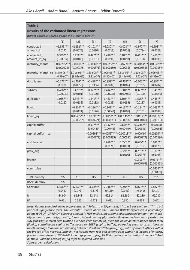
3.2. FindingsThe first model using bank dummies gives an indication of the impact of contract attributes on spreads. Based on the results of the model (Table 1, model (1)), the higher the contract amount and the longer the maturity, the smaller the spread above the BUBOR. However, this effect only applies until a certain level, as shown by the positive sign of the squared variables. The significance of the loan amount

11 The subsidy is differentiated depending whether the loan’s purpose is to purchase used or new property. In the latter case, the number of children in the household also influences the subsidy. However, these two pieces of information are not available, so we assumed that every loan was contracted to purchase a used home. Based on aggregate statistics, this assumption will not lead to any significant errors, in view of the fact that only a small fraction of newly extended loans were used to purchase new homes in 2014-2015 (MNB 2016).

16 Studies


is presumably explained partly by the impact of income as an unobserved variable: wealthier borrowers, representing a lower risk tend to purchase larger properties which calls for higher loan amounts. Economies of scale considerations may also have an impact: every loan contract comes with certain fixed costs (such as communicating with the customer, handling payment difficulties), which requires a higher spread on smaller credit amounts. However, above a certain level, potential loss rises and this is reflected in the spread. For maturity, the negative coefficient may capture the effect of shrinking credit risks through the decreasing payment-to-income ratio. This effect however is offset by growing liquidity risks for loans with very long maturities, so as the maturity grows longer, a higher spread is warranted.

As suggested by intuition, the collateralized nature of a loan decreases the spread, while interest rate fixation of over one year increases the spread above the interbank rate. Based on the estimate, the state subsidy also has a relevant impact. In the database, we were able to observe the total interest rate received by the bank, which incorporates state subsidies received as well. We are able to estimate the approximate size of the subsidy based on the rules of the Home Creation Scheme being in effect in 2014–2015, and thus are also able to observe whether the bank prices subsidised loans differently depending on the amount of subsidy. Our findings show that for 1 percentage point of state subsidy, banks apply interest rates that are over 0.3 percentage points higher on average, ceteris paribus. The customer still fares well, getting the loan at a spread that is 0.6 to 0.7 percentage point smaller than the market rate in case of a 1 percentage point subsidy, while the bank “keeps” 30–40 per cent of the subsidy. This finding may also give an indication of the level of competition.12

Based on the coefficients identified above, changes in the general contract characteristic of newly extended loans over the past two years have pointed towards a reduction in spreads above the BUBOR. Since 2014, both the average of the contracted amount and the average maturity have increased, while the proportion of subsidised loans and the amount of state subsidy have continuously decreased, due to the characteristics of the pertaining regulation,13 falling to minimal levels by 2015 (from February 2015, the average market interest rate was below the 6 per cent corresponding to the lower threshold of the state subsidy). These three

12 Besides a low level of competition, it may of course reflects the impact of unobserved variables characterising various bank portfolios, that has been left out from the model. For example, if a bank specifically targets risky, lower-income customers with its state subsidised schemes, the higher spreads are indeed warranted. However, the fact that borrowers are aware of state subsidy options and may specifically seek them out irrespective of their income status decreases the probability of this distortion. However, the restrictions of subsidisation pertaining to property value increase the risk of bias.

13 According to the rules of the Home Purchase interest subsidy, the interest rate payable by the customer must be no less than 6 per cent, so the subsidy can only lower the interest rate to this threshold. Given that market interest rates approached and even dipped below this level, the state subsidy lost much of its relevance compared to earlier, reflected in the shrinking ratio of subsidised loans.

17


characteristics have all fostered a reduction in transactional interest rates, and thus spreads.

For the model supplemented with bank variables, the signs of the coefficients discussed so far do not change, and they retain similar orders of magnitude (Table 1, models (2)-(7)). For bank variables, the credit losses of recent years and higher operating costs were generally associated with larger spreads, which is in line with our preliminary expectations and the findings of the international literature. The ratio of net income from fees and commissions within net income of interest, fees and commissions has a negative coefficient, which suggests that banks which generate income through other channels — for instance by selling other services alongside loans — may take this into account by decreasing spreads. The ratio of liquid assets relative to total assets had a negative impact on spreads in the two years under review, which may capture the price-reducing effect of growing credit supply, while the positive coefficient of the capital buffer coefficient may reflect the impact of higher cost of capital. The latter variable, however, loses its significance in the broadest specification. For both variables, the square values mostly have an opposite sign (with the exception of the capital buffer, where the sign is the same in the broadest specification, albeit the value of the coefficient is particularly low), so these effects also only apply up to a certain level. The ratio of branch offices within the banking system branch office network has a positive coefficient, which may capture market power: banks with relatively more branch offices may have nearly exclusive presence on a greater amount of local markets, which they may then enforce in their pricing. We address this effect in depth in the section on the model examining demand patterns (Chapter 5).

18 Studies


Table 1Results of the estimated linear regressions (target variable: spread above the 3-month BUBOR)

(1) (2) (3) (4) (5) (6) (7)contracted_ amount_ln

–1.655***(0.0171)

–2.131***(0.0675)

–2.101***(0.0680)

–2.030***(0.0713)

–2.008***(0.0716)

–1.977***(0.0724)

–1.993***(0.0727)

contracted_amount_ln_sq

0.335***(0.00512)

0.421***(0.0188)

0.422***(0.0191)

0.410***(0.0196)

0.406***(0.0197)

0.411***(0.0198)

0.416***(0.0198)

maturity_month –0.00265***(0.000278)

–0.00608***(0.000376)

–0.00588***(0.000371)

–0.00282***(0.000359)

–0.00271***(0.000358)

–0.00344***(0.000355)

–0.00339***(0.000354)

maturity_month_sq 8.57e-06***(6.79e-07)

1.71e-05***(8.92e-07)

1.63e-05***(8.82e-07)

1.00e-05***(8.50e-07)

9.81e-06***(8.49e-07)

1.11e-05***(8.42e-07)

1.09e-05***(8.39e-07)

d_collateral –0.777***(0.0200)

–1.409***(0.0358)

–1.498***(0.0356)

–0.899***(0.0287)

–0.928***(0.0286)

–1.007***(0.0285)

–0.994***(0.0287)

subsidy 0.436***(0.00930)

0.423***(0.0101)

0.372***(0.0100)

0.414***(0.00932)

0.381***(0.00944)

0.327***(0.0100)

0.345***(0.00999)

d_fixation 1.085***(0.0127)

1.343***(0.0132)

1.341***(0.0132)

1.483***(0.0139)

1.504***(0.0139)

1.515***(0.0137)

1.485***(0.0136)

liquid

–0.304***(0.0121)

–0.286***(0.0126)

–0.162***(0.00849)

–0.137***(0.0101)

–0.124***(0.0101)

–0.0697***(0.0109)

liquid_sq

0.00405***(0.000209)

0.00396***(0.000221)

0.00157***(0.000141)

0.00145***(0.000180)

0.00112***(0.000180)

0.000379**(0.000193)

capital buffer

0.137***(0.00480)

0.142***(0.00442)

0.147***(0.00449)

0.0238***(0.00545)

-0.000334(0.00561)

capital buffer__sq

–0.00505***(0.000379)

–0.00597***(0.000339)

–0.00713***(0.000357)

0.000494(0.000374)

0.00205***(0.000396)

cost to asset

0.678***(0.0171)

0.550***(0.0173)

0.675***(0.0182)

0.636***(0.0176)

prov_avg

0.327***(0.0100)

0.281***(0.00976)

0.370***(0.0108)

branch

0.0303***(0.000762)

0.0375***(0.000862)

comm_fee

–0.0350***(0.00178)

TIME dummy YES YES YES YES YES YES YESBANK dummy YESConstant 6.426***

(0.0421)12.62***(0.173)

11.68***(0.177)

7.748***(0.129)

7.091***(0.141)

6.877***(0.141)

6.822***(0.147)

N 64,904 62,848 62,848 62,814 62,280 62,280 62,280R2 0.671 0.562 0.572 0.621 0.630 0.638 0.641

Note: Robust standard errors in parentheses.* Refers to a 10 per cent, ** to a 5 per cent, and *** to a 1 per cent significance level. The variables: spread above the 3-month BUBOR expressed in percentage points (BUBOR_SPREAD), contract amount in HUF million, logarithmised (contracted amount_ln), matu-rity in months (maturity _month), loan collateral dummy (d_collateral), estimated amount of state sub-sidy (subsidy), interest rate fixation over one year dummy (d_fixation), liquid assets/balance sheet total (liquid), consolidated capital buffer based on SREP (capital buffer), operating costs to assets (cost to asset), average loan loss provisioning between 2008 and 2014 (prov_avg), ratio of branch offices within the branch office network (branch), net income from fees and commissions within net income of interest, fees and commissions, 2008–2012 average (comm_fee), TIME dummies and institution dummies (BANK dummy). Variables ending in _sq refer to squared variables.Source: own calculations.

19


4. identifying supply effects using the panel model

4.1. database and methodologyWe also used a panel database for our analysis, compiled from Hungarian banking system data that includes data on the major banks involved in housing lending in Hungary between 2004 Q1 and 2014 Q4 (OTP Bank, MKB Bank, Budapest Bank, FHB Bank, Cetelem Bank, Erste Bank, Raiffeisen Bank, CIB Bank, Unicredit Bank and K&H Bank).14 Our approach was to use a regression model expressed for the differences of the dependent variable and that of the explanatory variables (3). We estimated a model using fixed effects broadly employed in the literature15, and a dynamic model also containing the dependent variable’s lag, used more rarely (e.g. Valverde – Fernández 2007).16

Because the presence of unit root processes could not be ruled out for level time series and because error terms exhibited autocorrelation when applying the fixed effect model, we instead chose to use a static model containing the first differential of the variables:

Δyit = ΔXit' β +eit (3)

eit =δ t +ω it (4)

ω it ∼ I.I.D. , (5)

Where Δyit is the annual change in housing loan margins, ΔXit is the annual change in explanatory variables and δt is the time fixed effect . Because our panel is balanced, the calculation of differences did not cause any significant data loss. In the following section, we present the findings of the model estimates, which proved relatively robust for several specifications.

4.2. FindingsThe database allows the examination of bank-specific factors shaping banks’ pricing decisions such as operating and funding costs, economies of scale and bank strategy. Because similarly to the previous database, the sample only includes Hungarian

14 The housing loans offered by one bank are special in that they are tipically unsecured transactions concluded for “other” loan purposes, and as such, can be regarded as consumption rather than housing loans. For this reason, we also made the estimate with the omission of this bank and our results proved to be stable.

15 Based on the tests performed using the fixed effect model, we cannot exclude the presence of unit root processes for certain variables, so we rejected this approach due to potential spurious regression bias.

16 Including the dependent variable lag may be motivated by the rationale that when determining bank lending spreads, earlier periods may serve as an anchor, and additionally, banks are not really capable of reacting flexibly when pricing loans due to market circumstances. Another advantage of this approach is its capacity to address the endogeneity stemming from reverse causality, which in our case may emerge in the variables related to bank portfolio structure or in the NPL ratio. But because the Blundell-Bond and Arellano-Bond type methods available for short time series can be applied effectively mainly with large cross section element numbers, in our case, estimating too many instruments created issues. Although we tried out different dynamic models, we encountered troubles with model diagnostics every time.

20 Studies


data, there is still no way to conduct a direct international comparison. However, the 10-year horizon allows us to control for country-level cyclical macroeconomic developments. In order to capture macroeconomic developments, we included annual GDP in the model and also included time fixed effects in an alternative specification (Model 2). Among the variables used, the ones capturing credit losses, such as the ratio of non-performing loans, the loan-to-value ratio and loan loss provisioning, can be considered as cyclical as well. We also included indicators representing market power for the sake of capturing structural effects: the size of bank branch networks and bank market share within household lending.

The findings of the estimated model have limited reliability. The sign of key variables is generally identical to the ones dictated by economic theory, but significance levels are not stable across the different specifications. Because banks are often unable to adapt on a quarterly horizon, we consider the findings of the model expressed for annual variables as the most convincing, so the following section addresses these in detail (Table 2). Overall, from our findings indicative conclusions can be drawn on the factors that shape housing loan spreads in the Hungarian banking system.

21


Table 2Results of the Hungarian bank panel model (target variable: spread above the 3-month BUBOR)

VARiABLES (1) (2)

Operating cost 0.994(0.779)

0.489(1.086)

Other income/interest revenue –0.00831(0.00604)

–0.00346(0.00632)

Liquidity 0.0470***(0.0174)

0.0508***(0.0183)

CAR 0.0376**(0.0165)

0.0995***(0.0350)

Ratio of fixed-rate loans slope of the yield curve 2.774***(0.699)

3.469***(1.105)

External liabilities 0.0206(0.0267)

0.00873(0.0283)

GDP (YoY) –0.188***(0.0633) –

LTV 0.0128*(0.00706)

0.00851(0.00775)

NPL 0.120***(0.0364)

0.0882**(0.0393)

Provisions 0.389***(0.124)

0.209**(0.101)

Proportion of branches 0.141*(0.0786)

0.124*(0.0683)

Market share 32.44(19.84)

35.80(21.84)

Constant 0.0636(0.211)

1.427*(0.849)

Time fixed effect – YES

Number of observations 317 317

R-squared 0.22 0.34

Number of banks 10 10

Note: robust standard errors in parantheses.* Refers to a 10 per cent, ** to a 5 per cent, and *** to a 1 per cent significance level.Variables: operating cost to balance sheet total, non-interest income/interest income, liquid assets/balance sheet total, capital adequacy ratio expressed as a percentage, the share of fixed loans multipli-ed by the slope of the yield curve (5-year government security yield – 3-month BUBOR) taken into account after 2010, the share of external liabilities within the sum of deposits (households and corpora-te) and external liabilities, GDP growth expressed in percentage points, loan value to the property pledged as collateral expressed as a percentage, share of non-performing loans in proportion to house-hold and corporate loans, loan loss provisioning in the given period in proportion to the balance sheet total expressed as a percentage, market share within the stock of outstanding household loans. We included the annual change of each factor into the model. Because it takes different amount of time for the changes of various factors to become incorporated into spreads, we applied an annual lag for ope-rating costs and a quarterly lag for the capital adequacy ratio, the non-performing loan ratio and the provision. Source: own calculations.

22 Studies


The individual bank factors capture, among others, the difference between banks’ business models. The coefficient of the share of operating costs to balance sheet total is not significant, so in this model, we are unable to reliably confirm the intuition that banks compensate higher operating costs with setting higher prices.17 However, this result can also be distorted by the change in the ratio’s denominator (e.g. as a result of deleveraging after the crisis). The ratio of other income to interest income is also not significant at the usual significance levels. We featured this variable in the model to be able to control for bank strategies that place greater emphasis on net income from fees and commissions, allowing the bank to offer more attractive lending rates. The positive sign of the share of liquid assets to the balance sheet total and the capital adequacy ratio suggest that banks incur additional costs to maintain excess liquidity and excess capital which they compensate with higher prices.18 We examined the ratio of fixed rate loans on variable interest rate loans for the post-crisis period in interaction with the slope of the yield curve. Based on our expectations, at those banks where the ratio of fixed interest rate loans is higher, the aggregated spread is sensitive to the slope of the yield curve which captures the higher cost of funding and/or the interest rate risk. This impact was significantly identified during the panel estimate on Hungarian banks. We included the variable of the share of external liabilities to corporate and household deposits in the regression in order to control for the difference in business models among banks which are relying on and those which are not relying on external funds. This variable is not significant, that is, the results of the regression do not suggest that banks would price differently as a result of their reliance on external funds.

Among cyclical variables, we go into detail about the impact of both the macro variables and that of the individual bank variables related to the cyclical position. The negative coefficient estimated for GDP capturing the economic performance suggests the pro-cyclical nature of spreads. In the case of an economic contraction, spreads increase in line with high risks as a sign of decreasing credit supply, which further aggravates the contraction of the economy, while during a boom period, banks lend with more moderate spreads, thereby further strengthening growth. The LTV ratio entered in the regression with a positive sign. The higher LTV ratio reflects higher risk, since in the case of default the bank may mitigate or avoid credit loss by selling the collateral. It should be noted that banks can compete not only in price,

17 What makes the identification of the impact of operating costs more difficult is that prior to the crisis several banks gained market share through agent sales, the cost of which — as opposed to operating their own branch network — did not appear among their operating costs. Considering that following the onset of the crisis, agent sales decreased significantly, this may also be the reason why operating costs still appear as a significant factor in the case of a micro-level database only building on data from 2014-2015.

18 In the case of liquidity, this result contradicts the result of the estimation conducted on the micro-database. However, t the latter database covers only a two-year period while the panel database processes the data of one decade, which means a difference. On the other hand, the impact of capital adequacy is in line with the results of the micro-database.

23


but also in lending conditions, which may cause endogeneity for the LTV variable, that is, in this case, the underestimation of the coefficient, especially if we examine newly issued loans. The non-performing loan ratio within the loan portfolio of the private sector (NPL) also correlates with the economic cycle: during the period of an economic boom the share of the NPL portfolio is generally low, while during recession, this ratio increases. The high NPL captures both already written-off and potentially expected lending loss; accordingly, the sign of the variable is positive in the estimated model. Similarly to the non-performance ratio, provisioning also reflects the risks, but this indicator only includes the loss already written off by the bank. The sign of the impairment is also positive in the model.

Because the development of economic growth in other countries was similar to the Hungarian trend, the cyclical variables probably only explain some of the difference between spreads in the region. In our view, some structural reasons are also causing the high spreads. We attempted to capture these factors by the share of the number of bank branches and the banks’ market share on the household credit market. The share of the number of bank branches in comparison to the number of branches of the banks included in the model not only takes into account the bank’s own branch network, but also the size of that branch network compared to that of the competitors. This variable is significant and it is featured in the model with a positive sign which suggests that banks operating a large branch network are able to use their dominant position on the market when defining the spreads on mortgage loans. In our view, the role of the branch network is indeed relevant because the majority of the population can select only from a limited number of banks located near their place of residence, which decreases competition between banks. The market share variable is not significant, so this simple control variable does not confirm our impression that banks strive to use their dominant position on the market in their pricing.19

It may be a question whether the levy on banks increased margins after it was introduced. We are unable to analyse this impact on the micro data due to the short time period available, but we have included it in the panel model as an explanatory variable. Based on our results, the impact of the bank levy is not apparent among new loans, which also confirms the findings of the literature according to which banks have averted this extra cost by modifying the interest rate of their existing loan portfolios (Capelle-Blancard – Havrylchyk 2013).

19 We can see in the correlation matrix included in the annex that there is high correlation between the share of branches and the market share variable. For this reason, we decided to apply the model without this latter variable, and the significance level and the coefficient of the branch-proportion variable did not change significantly either.

24 Studies


5. identification of demand effects using micro-level data20

5.1. database and methodology21

Along with supply factors, it is important to examine whether the demand side supports the existence of a competitive market or whether there are any frictions that could result in less competition. As part of this investigation, we developed a model which belongs to the family of discrete choice models. This allows us to examine the factors that influence consumers in bank selection. During the modelling, we relied on the Central Credit Register database which contains detailed loan analytics for new disbursements, including customer characteristics, from 2015 onwards. The final model contains the data of seven major banks, covering more than two thirds of the mortgage loan market. In the following, we present the intuition behind the model and the main steps of the estimation (estimating interest rates and restricting the choice set) and we summarise the results of the estimation.

We applied a multinomial regression model for the analysis, placing consumers’ individual choices into the focus of the investigation. Factors influencing the decisions of consumers can be classified into three groups. First, the conditions of the selected loan product and the characteristics of the selected bank play a key role. Beside the interest rate, we can mention the factors that capture the quality of bank services and that a past relationship with a given bank may also be an important aspect. Second, the customer’s taste also matter as the popularity of the banks may differ in the various segments of the society. Third, the customer-specific factors which are not observable by the researcher show up in the error term of the estimate. Based on the above, following Train’s demonstration (2002), the utility of the customer by choosing a given bank can be written as:

Uij =Vij xij ,si( )+ ε ij , (6)

Where Uij is the utility of consumer i if he chooses bank j, xij is the vector containing variables which are customer- and also bank-specific (e.g. transactional interest rate). si is the vector that contains solely customer characteristics (e.g. age, income) while εij is the model’s error term, which follows an i.i.d. extreme value distribution by assumption. The model’s starting point is that customers strive to maximise their utility, that is, they opt for the offer promising the highest level of utility compared to other offers.

Uij >Uik , ∀j ≠ k (7)

20 This chapter provides a brief summary of the study, which was presented on the conference entitled „5th EBA Policy Research Workshop: Competition in Banking: implications for financial regulation and supervision” (Aczél 2016).

21 The above study presents in detail the steps of database cleaning and the descriptive statistics of the data used.

25


Approaching the observable part of the utility function with a linear relationship, we have:

Vij = xij' β +Dj'γ si , (8)

where β is the parameter vector belonging to the characteristics of the various alternatives, Dj is a vector containing binary variables denoting individual banks, γ is the matrix containing the parameters belonging to the customer characteristics differing by bank. Using all of the above and assuming that the error term follows an i.i.d. extreme value distribution, the likelihood that customer i selects bank j can be written as:

Pij =

exij' β+Dj'γ si

exik' β+Dj'γ sik∑

(9)

To estimate the model, we also need theoretical interest rate data that show the interest rate at which the customer would have received a loan had he chosen another bank instead of the observed choice. We estimated these theoretical interest rates using linear regression, so that we created a unique model for every bank where the dependent variable is the interest rate and the explanatory variables can be classified into two groups. First, we included in the models the characteristics of customers who actually borrowed from the specific bank (age, location, income) and second, we also controlled for the transaction attributes (value of the mortgage, maturity, loan type). The explanatory powers of the models are high (R2 around 0.9) and their standard error is low (around 0.3 percentage points).22 Despite the good model statistics, the fact that this estimation may be biased is an issue. The potential bias stems from the fact that the estimation sample is not random, because banks may be chosen by customers with strongly diverging characteristics (self-selection bias). However, it is important to stress that this estimation procedure is similar to the procedure applied by banks, because banks themselves define their pricing models based on relationships estimated with regard to their own clientele. In our view, our estimated models feature acceptable accuracy and estimate for a sample similar to banks’ samples, so these estimates provide a good approximation of the theoretical interest rate that banks have offered to prospective borrowers.

After estimating theoretical interest rates, we also examined whether the assumption that households can choose from the offerings of all banks is well-founded. We found that households faced both geographic and financial constraints, so it is likely that they can only choose from a narrow range of banks when making mortgage loan decisions. The geographic constraints are reflected in the fact that

22 R2 (0.32) is low for a single bank interest rate model, however this model also yielded an estimate with a low error (RMSE 0.33).

26 Studies


no more than two of the eleven major banks are present in half, and no more than four are present in three-fourths of Hungary’s districts (Figure 6).23

Figure 7 captures the differences in banks’ business strategies through the distribution of customer income associated with the loans extended in 2015. The figure clearly shows that the banks marked by black mainly serve low-income customers, while those marked by red mainly target higher-income customers and barely lend to lower-income segments, or not do not lend to these segments at all. The distribution of loan size or the value of the property to be purchased shows a similar picture. We used these findings within the models to restrict the group of banks that customers may choose from.

23 The distribution of bank presence as a function of the population would be an interesting addition. More than a quarter of the Hungarian population lives in a district where there are no more than two banks, and nearly 40 per cent lives in a district where there are no more than four banks present from among the eleven major banks. Only half of the population has access to at least six major banks in their region.

Figure 6distribution of the number of banks present in various districts

0

25

50

75

100

0

20

40

60

80

1 2 3 4 5 6 7 8 9 10

Per cent

Num

ber o

f dist

ricts

Number of banks in districts

Number of districtsCumulative share of districts (right-hand scale)

Source: MNB.

27


5.2. FindingsWe run the final model in eight specifications; the results are listed in Table 3. In the first specification, we neither controlled for choice sets nor included demographic variables (A1). The findings of this estimate are not in line with expectations, because for example the interest rate coefficient is positive, which is difficult to interpret, as it suggests that consumers like high interest rates. This finding also suggests that endogeneity distorts estimates, which may be because the impact of demand and supply is not adequately distinguished in this specification.

For the sake of ruling out endogeneity, we implemented three changes in the model. First, we incorporated demographic variables and bank dummies (A2, A4, B2, B4), second, we restricted the choice sets (B1-B4), and third, we incorporated a variable that captures previous relationship with banks (A3, A4, B3, B4). We obtained intuitive results in each case, and the sign of the interest rate is negative, which is in line with a negatively sloping demand curve.

In the models that included demographic variables and bank dummies (A2, A4, B2, B4), the issue of endogeneity was significantly reduced. The procedure applied addresses the typical problem of a bank taking advantage of its strong brand and

Figure 7distribution of incomes behind the loans extended by the seven major banks

0

5

10

15

20

25

30

35

0

5

10

15

20

25

30

35Per cent Per cent

50,0

00

100,

000

150,

000

200,

000

250,

000

300,

000

350,

000

400,

000

450,

000

500,

000

550,

000

600,

000

650,

000

700,

000

750,

000

800,

000

Income (HUF)

Note: The various lines indicate the banks included in the analysis.Source: MNB.

28 Studies


lending at high interest rates in response to strong demand. Another key finding is that by including demographic variables, clearly outlined taste patterns can be identified. A good example of such pattern is that based on the estimated coefficients, older age groups tend to prefer banks that have an established presence on the Hungarian market, while younger age groups prefer newer market entrants.

The models estimated by narrowing the choice set (B1-B4) may yield a more realistic picture because banks that are not potential choices for customers are left out of the calculations. Thus for instance, in the case of a low-income customer, obtaining a loan from a bank that exclusively targets an affluent clientele and offers low interest rates is not a realistic option. If we leave out this bank from the customer’s potential options, it would lead to the false conclusion that although the customer could borrow at a low interest rate, he instead chose to borrow at a higher rate. This effect may be present in specification A1, where we did not control for the choice sets. A key finding is that narrowing the options alone results in the estimation of a demand curve with a negative slope (B1).

We also included a variable in the models that shows whether the customer has borrowed from a specific bank (in the past eight years). This variable is significant and positive in every specification (A3, A4, B3, B4), which suggests that customers prefer banks that they are familiar with in their borrowing decisions.

In every model, we included a variable among explanatory variables that shows the number of branch offices that the bank has in the region where the customer resides. This variable is also significant and positive in almost every specification, meaning that an expansive branch network is valued by customers.

Overall, the estimation results suggest that the Hungarian population tends to choose from a specific and narrow range of banks when making borrowing decisions. This is partly due to the geographic distribution of banks’ branch networks and partly to the taste patterns prevailing within society; banks’ business models are also relevant. These limitations and patterns allow banks to price their products according to oligopolistic competition. These findings confirm the outcomes of the bank panel model investigating supply effects, i.e. that the distribution of branches plays a key role in determining spreads. Finally, these estimates demonstrate that structural factors play an important role on the Hungarian mortgage market.

29


Table 3Results of the demand model estimate

Total choice set Restricted choice set

No taste(A1)

Taste(A2)

No taste(A3)

Taste(A4)

No taste(B1)

Taste(B2)

No taste(B3)

Taste(B4)

Interest 0.171*** –1.262*** –0.0176 –1.182*** –0.862*** –1.640*** –1.042*** –1.539***

Number of branches

0.0221*** 0.000881 0.0136*** 0.00213** 0.0181*** 0.00762*** 0.00843*** 0.00971***

History 3.037*** 2.750*** 2.502*** 2.750***

Bank A

Age 0.00311 0.00563 0.00956 0.0167**

Income 1.142*** 1.213*** 0.401*** 0.430***

Constant –6.447*** –6.015*** –2.614*** –1.945***

Bank B

Age –0.0266*** –0.0115** –0.0153 –0.00750

Income 1.326*** 1.332*** 0.428*** 0.425***

Constant –10.22*** –9.233*** –3.936*** –2.947***

Bank C

Age –0.0155*** –0.00626** –0.0149*** 0.00206

Income 0.979*** 1.032*** 0.439*** 0.441***

Constant –3.337*** –2.895*** –1.705*** –1.195***

Bank D

Age –0.0623*** –0.0511*** –0.0747*** –0.0632***

Income 1.270*** 1.289*** 0.523*** 0.515***

Constant –5.198*** –4.584*** –0.590* 0.283

Bank E

Age –0.0165*** –0.00558* –0.0180*** –0.00227

Income 0.480*** 0.540*** 0.0768** 0.146***

Constant –2.626*** –2.676*** –1.362*** –1.509***

Bank G

Age 0.00544 0.0136*** 0.00448 0.0129*

Income 1.245*** 1.275*** 0.504*** 0.502***

Constant –7.052*** –6.388*** –2.897*** –1.948***

Note: * Refers to a 10 per cent, ** to a 5 per cent, and *** to a 1 per cent significance level.Source: own edit.

6. Why are the spreads so high?

In previous sections we listed a number of characteristics that may potentially explain the high Hungarian spreads. In line with our research strategy, in the first step we attempted to explain the heterogeneity of Hungarian banks’ price setting behaviour by using bank-level and customer-level variables. The next step is to examine the performance of the Hungarian banking sector compared to international examples with respect to the significant variables identified in the models estimated on the Hungarian sample.

30 Studies


Our main findings, as presented in previous sections, were the following:

• Through a composition effect, the higher share of contracts with an initial interest rate fixation of over 1 year may account for the higher level of Hungarian spreads. The slope of the yield curve may also contribute to the relatively high cost of fixed-interest loans.

• An increase in GDP typically reduces spreads, while recession raises them.

• Credit losses and the higher share of nonperforming loans may influence the spreads through higher risk costs, partly as a result of banks’ propensity to build on historical credit experiences involving past – poor quality – loans.

• Higher operating costs have been coupled with higher spreads in recent years.

• The lower share of profits from fees and commissions may induce relatively higher spreads.

• Similarly, banks’ capital adequacy (capital requirement) may also exert upward pressure on spreads.

• There is a positive correlation between the average loan-to-value ratio of the loans disbursed and the spread imposed.

• Banks representing a higher share in the branch network of the banking sector applied, ceteris paribus, higher spreads.

• The lack of a sufficient number of market participants in certain regions and debtors’ taste patterns may lead to the emergence of an oligopolistic market.

Unfortunately, owing to the limited availability of data, only some of these items can be analysed in international comparison. In the following, we focus our research on items that – in light of the international literature and/or our estimated models – appear to be especially important, and for which relevant international data are also available. The latter may pose a problem mainly in relation to the results of the demand model; indeed, there is practically no information available at the international level on debtors’ income status, their taste and on the distribution of branches. We will not go into detail about the topic of liquid assets and the loan-to-value ratio because – although we found some evidence that these indicators and the size of the spreads are positively correlated – international literature does not provide clear guidance on the impact of such attributes on spreads.

31


6.1 Ratio of loans with an initial interest rate fixation of over 1 yearAs pointed out above, the outstandingly high Hungarian spreads observed at the end of 2015 and in early 2016 can be primarily attributed to the higher spread on loans with an initial interest rate fixation of over 1 year. The spread between these lending rates and the interbank rate is partly determined by the yield curve; indeed, in the case of a steeper (and upward sloping) yield curve, the creditor bank will also face increased costs of funds when borrowing funds with a long-term initial rate fixation and consequently, this premium will be priced into the bank’s lending rate. If the bank relies on short-term and/or floating rate funds to finance loans extended with a long-term rate fixation, the interest rate risk thus incurred by the bank justifies an increase in the spread. Based on Eurostat data, the yield curve is relatively steep in Hungary compared to other EU countries. At the end of 2015, the spread between the ten-year government bond yield and the three-month interbank interest rate took the fifth highest value in Hungary.

Figure 8Share of housing loan contracts with an initial interest rate fixation of over 1 year in new disbursements vs. the interest spread between contracts with long-term and short-term interest rate fixation

RO

HU

SI

UK

IE

SE

ES

NL

IT

DK

DE

CZ

BE SK

0

10

20

30

40

50

60

70

80

90

100

–1.0

–0.5

0.0

0.5

1.0

1.5

2.0

2.5

Shar

e of

con

trac

ts w

ith a

n in

itial

fixa

tion

perio

d of

m

ore

than

1 y

ear (

2015

Q4,

per

cen

t)

Difference of average interest rates of contracts with an initial fixationperiod of less then 1 year and more than 1 year (2015 Q4, percentage points)

Note: In the case of loans with an initial interest rate fixation of over 1 year, the most widespread scheme – the 1Y–5Y initial rate fixation – was considered. Source: European Mortgage Federation, national central banks.

32 Studies


As at end-2015, data reveal that in Hungary, the share of products with a rate fixation of over 1 year was high even though Hungary recorded one of the highest interest spreads between fixed and variable rate products (Figure 8). It should be noted that, if the interest rate spread between two product types reflects the expected interest rate path, in theory, choosing between the two products would not make any difference for a rational consumer, provided that his interest expectations coincide with market expectations. Experience, however, shows that instead of looking at the interest rate path as a whole, consumers are far more concerned about the interest rate spread prevailing at the time of the loan disbursement and during the short period that follows (Johansson et al. 2011; Badarinza et al. 2014; Holmberg et al. 2015). It should also be remembered that, as noted in the introduction, it is often the given country’s lending “traditions” or institutional background that determine consumers’ decisions as they select from the product types available. Having said that, since the surge in household lending at the beginning of the 2000s, it has only been observed in recent years

Figure 9Share of housing loan contracts with an initial interest rate fixation of over 1 year in new disbursements vs. the adjusted interest spread between contracts with long-term and short-term interest rate fixation (2015 Q4)

RO

HU

SI

UK

IE SE

ES

NL

IT

DK

DE

CZ

BE SK

0

10

20

Difference of average interest rates of contracts with an initial fixation period of less then 1 year and more than 1 year, adjusted by the difference caused by expected change in interest rates (2015 Q4, percentage points)

30

40

50

60

70

80

90

100

–1.5

–1.0

–0.5

0.0

0.5

1.0

1.5

Shar

e of

con

trac

ts w

ith a

n in

itial

fixa

tion

perio

d of

mor

e th

an 1

yea

r (20

15 Q

4, p

er c

ent)

Note: In the case of loans with an interest period of over 1 year, the most widespread scheme – the 5Y–10Y initial rate fixation – was considered. We deducted the difference between the 5-year IRS and the short-term interbank interest rate from the difference between the average interest rate on fixed-ra-te and variable-rate transactions.Source: European Mortgage Federation, Datastream, national central banks.

33


that households are more likely to become indebted with fixed interest rates, on a market basis (without any state subsidy).

We also analysed the figure above after adjusting the interest spread by the differential between the 5-year interest swap relevant to the given currency and the short-term interbank interest rate. Our goal was to exclude, as far as possible, the effect of interest rate path expectations from the premium shown in the figure, in order to obtain a better approximation of the “pure” differential concerning the rational consumer.24 Based on the values thus received, in Hungary the premium on fixed-interest loans is higher than would be warranted by the difference between funding costs; consequently, we still cannot consider the increase in the share of fixed-rate loans as being trivial (Figure 9).

We believe that the substantial share of fixed-rate products suggests that the Hungarian population is more risk averse than borrowers in other countries; indeed, Hungarian customers are willing to pay a much higher premium for a fixed interest rate. This, in itself, does not imply that this premium (or at least a part of it) is not justified; it is an interesting development, however, that Hungarian household debtors are apparently more likely to pay a considerably larger sum in exchange for a smaller deviation in monthly payments. In our opinion, this may also reflect households’ negative experiences with foreign currency loans and the extremely volatile instalment amounts associated with them. Banai and Vágó (2016) also confirm that foreign currency lending gave rise to precautionary motives among households: based on data derived from the Austrian central bank’s Euro Money Survey, the authors provided evidence that the negative experiences associated with foreign currency lending clearly set back credit demand. It is also conceivable that the “demand” problems presented in Section 5 can be perceived more strongly – possibly because of the limited number of active market participants – in the market of fixed-interest loans. The picture appears somewhat more complex once we consider that the high ratio of fixed-interest products has partly resulted from the activity of building societies issuing fixed-interest loans. Nevertheless, it is also true for these institutions that the interest rate they impose exceeds the interest level of variable-rate products; in other words, the customers of building societies will also pay the premium between the fixed rate and the variable rate in exchange for a predictable interest rate.

24 However, this method should be viewed as an approximation only; indeed, the differential between the average interest rate on actually disbursed fixed-rate loans and the interest rate on variable-rate loans can also be influenced by composition effects, especially when a particular product has gained dominance in the given country. Various sub-markets may be dominated by different creditors and borrowers and the different characteristics of these market participants may also be reflected in aggregate interest rates. Consequently, the “pure premium” could not be presented even on the second figure.

34 Studies


6.2. The role of credit lossesModel estimates have demonstrated that the ratio of credit losses and non-performing loans play a prominent role in credit spread developments. In calculating their rate of return, banks should consider the probability of a borrower’s falling into delinquency during the term of the loan, and calculate the expected recovery rate on the collateral in case of the borrower’s delinquency. The calculation of expected losses is based on historical data; consequently, a substantial non-performing portfolio may have a long-term impact on price-setting. Based on the distribution of NPL ratios, Hungarian banks are among the more affected institutions of the region, which may have contributed to the emergence of higher spreads (Figure 10).

Collateral recovery and the efficiency of enforcement proceedings play a key role in credit loss developments. Hungarian legislation has significantly hampered banks in the acquisition and sale of real estate property in recent years. Moreover, the legal environment protecting debtors motivated even performing debtors to suspend their monthly payments, generating even more credit losses for banks (Dancsik et al. 2015).

Figure 10distribution of banks by the ratio of non-performing loans in certain countries (2014)

0

10

20

30

40

50

60

0

10

20

30

40

50

60

GR

BG

SI

HU

RO

HR

IE

PT

LT

LV

PL

ES

AT

DK

BE

IT

SK

GB

CZ

LU

FR

NL

DE

FI

EE

SE

Per cent Per cent

Note: Columns indicate the 25–75th percentiles of the ratios of individual banking systems, while lines show the 10–90th percentiles. Countries are ranked in descending order based on the 75th percentile. Source: SNL Financial.

35


6.3. The role of operating costsOperating costs have an intuitive role in the evolution of spreads, as banks need to set a price that allows them to achieve profits. Banks’ lower efficiency and higher costs may also call for higher spreads. We demonstrated this effect successfully in the model featuring microdata; however, we did not receive significant results in the panel model. This may be partly attributed to the costs of agent sales preceding the outbreak of the crisis, as they were not part of banks’ operating costs.

Based on the international data available, the Hungarian banking sector is among the less cost-efficient banking systems (Figure 11). Obviously, the magnitude of operating costs cannot be fully separated from non-performing loans; indeed several items related to the management of the NPL portfolio raise the costs incurred by banks. Such costs include, for example, the need for personal treatment in the case of a bad loan, or the continuous safeguarding and potential upkeep of already recovered collateral.

Figure 11distribution of banks by the ratio of operating costs to risk-weighted assets in certain countries (2014)

0

2

4

6

8

10

12

0

2

4

6

8

10

12

SI

LU

LT

HU

BE

PL

DK

IE

ES

FI

DE

HR

IT

NL

GB

RO

AT

BG

FR

SK

GR

EE

CZ

LV

PT

SE

Per cent Per cent

Note: Columns indicate the 25–75th percentiles of the ratios of individual banking systems, while lines show the 10–90th percentiles. Countries are ranked in descending order based on the 75th percentile. Data may be biased due to the fact that the value of risk-weighted assets is sensitive to the methodology applied by the bank (standard or IRB method), but for lack of internationally available data, we are unable to assess the magnitude of this effect. In certain countries, there were few banks for which infor-mation was available and the distribution might only reflect the data of a single institution or an ext-remely limited number of institutions.Source: SNL Financial.

36 Studies


6.4. The role of net income from fees and commissionsAccording to the findings of the international literature, banks are more prone to set lower interest rates if they also collect income from services other than loan contracts. Although this was confirmed by the estimates we performed on microdata, it was not a significant variable according to the results of the panel model. In Hungary, the ratio of net income from fees and commissions is relatively small compared to other European countries (Figure 12), which may also contribute to higher spreads.

6.5. The role of capital adequacyOur models demonstrated that a higher stock of capital is generally associated with higher spreads. This effect has been identified in the international literature as well. Based on the CET1 (Common Equity Tier 1) ratio – which is composed of the best capital elements – Hungarian banks cannot be deemed overcapitalised by European standards (Figure 13). It hinders data comparability – especially in the case of CEE countries – that the capital position of a bank largely depends on the capital allocation strategy pursued by the non-resident parent bank, i.e. in which country the bank holds the buffer set aside on top of its consolidated capital requirement.

Figure 12Ratio of net income from fees and commissions to net income from interests, fees and commissions (2008-2013, mean)

0

5

10

15

20

25

30

35

40

45

50

0

5

10

15

20

25

30

35

40

45

50

LU

FR

IT

UK PT

LV

LT

PL

FI

DE

SE

AT

SI

HR

BE

ES

EE

CZ

RO

N

L BG

SK

DE

HU

IE

CY

GR

M

T

Per cent Per cent

Source: ECB Consolidated Banking Data.

37


It is not only the size of the capital buffer that is relevant to a bank’s capital position, but also the expected minimum statutory adjustment to its level. In parallel to the development of macroprudential strategy, regulatory authorities have gained access to several new discretionary instruments in recent years that exert an impact on banks’ capital position (systemic risk buffer, countercyclical capital buffer, capital buffer applicable to systemically important institutions). In Hungary, the level of the countercyclical capital buffer has remained at zero per cent since its introduction, but the other two instruments have higher levels. In our opinion, however, these rules cannot be a significant factor in the deviation of Hungarian spreads from the international average; first, because they are also used in other countries (ESRB 2016:52) and second, because banks are only required to comply with these two rules, for the first time, from 2017, which means that their effect must have been rather muted during our review period (2014–2015 and 2005–2014).

7. Conclusions

Hungarian banks apply a higher spread on housing loans than most of their European counterparts. This paper investigated the reasons for the high spread using econometric tools, along with simple statistical examinations. In the absence of a reliable, adequately detailed international database that covers a sufficiently

Figure 13CET1 capital adequacy ratio in international comparison (at end-2015)

0

5

10

15

20

25

30

35

40

0

5

10

15

20

25

30

35

40

EE

LT

IE

FI

LU

BG

LV

SE

MT SI

HR

RO

GR

DK

SK

CZ

CY

BE

DE

N

L PL

UK

HU

ES

AT

FR

PT

IT

Per cent Per cent

CET1 ratio

Source: ECB Consolidated Banking Data.

38 Studies


long time horizon, we attempted to identify the determinants of the spreads on the basis of Hungarian bank and transaction-level data. In the last step, we examined the Hungarian banking system’s sectoral performance relative to other European regions with respect to the main determinants identified.

Our results showed that the spreads diverging from those of the region are primarily caused by the higher spreads applied for loans extended with an initial interest rate fixation of over 1 year, while the spread on loans with short-term variable rates has already approached the regional average. Although the difference between the interest rates on variable and fixed-rate loans is relatively high in Hungary (partly as a result of the steeper yield curve), the share of loans with an interest rate fixation of over 1 year within newly disbursed loans is over 50 per cent. This means that borrowers are willing to pay a high premium in exchange for a fixed interest rate, even when adjusted for the higher costs associated with fixed-interest funds. Households’ negative experiences during the period of foreign currency lending may have been an important contributor to this risk aversion.

The ratio of non-performing loans, which is also high by international standards, may have been another factor in the emergence of high spreads. Banks set their spreads in consideration of the credit losses incurred, and higher credit risks are typically coupled with higher spreads. Through collateral recovery rates, the efficiency of the legal enforcement system may also play a role in the evolution of the spreads.

According to our estimates, the high share of operating costs may also induce higher spreads. Banks’ expected rate of return will warrant higher spreads if their cost-efficiency is inadequate. The relatively small impact of other net income items may also play a role: banks are more prone to set higher interest rates if they do not collect income from any other services. We could only demonstrate these last two effects in our estimates performed on microdata. Even in terms of these variables, the performance of the Hungarian banking sector is worse than the international average.

Our analysis also suggested that, owing to customers’ limited price flexibility and the geographical distribution of branches, competition is inadequate in the field of housing loans. Our demand model showed that, on the one hand, customers face geographical limitations: only a strictly limited group of banks has presence in many Hungarian administrative districts and customers tend to choose the easily accessible banks. On the other hand, banks’ business models also reduce the number of institutions that are perceived by consumers as potential opportunities; indeed, the banks which target affluent customers do not make efforts to serve low-income customers.

Thirdly, certain taste patterns suggest that customers rely on an extremely limited, preferred group of banks in making their borrowing decisions, and are only willing

39


to compare the offers of these chosen banks. These factors, overall, enable banks to set their prices in the context of oligopolistic competition. It is also a sign of weak competition that banks do not pass on to customers the full subsidy in the case of subsidised loans as they – according to our estimates – overprice these loans by about 30–35 per cent of the subsidy.

References

Aczél, Á. (2016): Who is interested? Estimation of demand on the Hungarian mortgage loan market in a discrete choice framework. 5th EBA Policy Research Workshop, under publication.

Badarinza, C. – Campbell, J.Y. – Ramarodai, T. (2014): What calls to ARMs? International evidence on interest rates and the choice of adjustable-rate mortgages. NBER Working paper, No. 20408, National Bureau of Economic Research.

Banai, Á. – Vágó, N. (2016): Drivers of household credit demand before and during the crisis. Manuscript. Magyar Nemzeti Bank.

Button, R. – Pezzini, S. – Rossiter, N. (2010): Understanding the price of new lending to households. Bank of England Quarterly Bulletin, 2010 Q3, pp. 172–182.

Capelle-Blancard, G. – Havrylchyk, O. (2013): Incidence of bank levy and bank market power. CEPII Working Paper, No. 2013–21. Centre dʼétudes prospectives et dʼinformations internationales.

Carlehed, M. – Petrov, A. (2012): A methodology for point-in-time – through-the-cycle probability of default decomposition in risk classification systems. Journal of Risk Model Validation, Volume 6. No. 3. Fall, pp. 3–25.

Dancsik, B. – Fábián, G. – Fellner, Z. – Horváth, G. – Lang, P. – Nagy, G. – Oláh, Zs. – Winkler, S. (2015): Comprehensive analysis of the non-performing household mortgage portfolio using micro-level data. MNB Occasional Papers, Special Issue. Magyar Nemzeti Bank.

Demirguc-Kunt, A. – Huizinga, H. (1999): Determinants of commercial bank interest margins and profitability: Some international evidence. World Bank Economic Review, Vol. 13, pp. 379–408.

Demirguc-Kunt, A. – Laeven, L. – Levine, R. (2003): The impact of bank regulations, concentration and institutions on bank margins. World Bank Policy Research Working Paper, No. 3030. World Bank.

ECB (2009): Housing finance the Euro Area. Occasional Paper, No. 101. European Central Bank.

40 Studies


EMF (2012): Study on mortgage interest rates in the EU. European Mortgage Federation.

EMF (2016): European Mortgage Federation Quarterly Review, 2016 Q1, European Mortgage Federation.

ESRB (2015): Report on residential real estate and financial stability in the EU. European Systemic Risk Board.

ESRB (2016): A Review of Macroprudential Policy in the EU in 2015. European Systemic Risk Board.

Gambacorta, L. (2014): How do banks set interest rates? NBER Working Paper, No. 10295. National Bureau of Economic Research.

Ho, T.S.Y. – Saunders, A. (1981): The Determinants of Bank Interest Margins: Theory and Empirical Evidence. The Journal of Financial and Quantitative Analysis, Vol 16, No. 4. Proceedings of the 16th Annual Conference of the Western Finance Association, pp. 581–600.

Holmberg, U. – Janzén, H. – Oscarius, L. – Van Santen, P. – Spector, E. (2015): An analysis of the fixation period for Swedish mortgages. Economic Commentaries, No. 7, pp. 1–19.

Johansson, J. – Lagerwall, B. – Lundvall, H. (2011): Larger share of variable mortgages – how does this affect the impact of monetary policy? In: Sveriges Riksbank: The Riksbank’s inquiry into the risks in the Swedish housing market. Sveriges Riksbank, pp. 97–108.

Laeven, L. – Majnoni, G. (2005): Does judicial efficiency lower the cost of credit? Journal of Banking & Finance 29, pp. 1791–1812.

MNB (2016): Housing Market Report. May. Magyar Nemzeti Bank.

Maudos, J. – De Guevara, F. (2004): Factors explaining the interest margin in the banking sectors of the European Union. Journal of Banking & Finance, No. 28, pp. 2259–2281.

Santos, C. (2013): Bank interest rates on new loans to non-financial corporations – one first look at a new set of micro data. In: Financial Stability Report 2013, Bank of Portugal, pp 127–134.

Saunders, A. – Schumacher, L. (2000): The determinants of bank interest rate margins: an international study. Journal of International Money and Finance, No. 19, pp. 813–832.

Train, K.E. (2002): Discrete Choice Methods with Simulation. Cambridge University Press. Cambridge.

Valverde, S.C. – Fernández, F.R. (2007): The determinants of bank margins in European Banking. Journal of Banking & Finance, No. 31, pp. 2043–2063.

41


Annex 1: Main descriptive statistics of transaction-based interest statistics

distribution of the sample by interest typeNumber of contracts distribution of contracts

Variable rate or initial fixation of up to 1 year

33,705 51.93

Interest rate with a fixation of over 1 year

31,199 48.07

Total 64,904 100

Source: MNB.

distribution of the sample by state subsidy Number of contracts Distribution of contracts

Market based 45,854 70.65

Subsidised 19,050 29.35

Total 64,904 100

Source: MNB.

descriptive statistics for interest rates and the spread over the three-month BuBOR interest rate (%) Spread over BuBOR (percentage points)

Mean Median 10th percentile

90th percentile Mean Median 10th

percentile90th

percentile

2014 Q1 7.9 7.7 5.7 9.7 5.1 4.9 3.0 6.9

2014 Q2 7.7 7.4 5.4 9.7 5.2 4.8 3.0 7.2

2014 Q3 6.8 6.6 4.7 8.5 4.6 4.4 2.5 6.3

2014 Q4 6.5 6.4 4.6 8.0 4.4 4.3 2.5 5.9

2015 Q1 6.3 6.2 4.6 7.7 4.3 4.2 2.5 5.6

2015 Q2 6.1 5.9 4.1 7.4 4.5 4.3 2.5 5.8

2015 Q3 5.7 5.3 3.6 7.2 4.4 3.9 2.2 5.9

2015 Q4 5.7 5.5 3.7 7.2 4.3 4.2 2.4 5.9

Total 6.4 6.3 4.2 8.5 4.5 4.4 2.5 6.3

Source: MNB.

42 Studies


descriptive statistics for the contracted amount and maturity by contracting quarter Contract amount (HuF millions) Maturity (months)

Mean Median 10th percentile

90th percentile Mean Median 10th

percentile90.

percentilis

2014 Q1 5.4 4.3 1.5 10.0 173.2 180.2 72.2 241.0

2014 Q2 5.8 4.5 1.5 10.0 172.1 180.2 72.4 241.0

2014 Q3 6.1 5.0 1.7 11.0 175.6 180.3 72.6 241.1

2014 Q4 6.1 5.0 1.9 11.5 180.2 180.4 72.9 241.7

2015 Q1 6.4 5.0 2.0 11.8 179.9 180.3 72.5 264.1

2015 Q2 6.5 5.0 1.6 12.5 175.3 180.2 71.0 265.2

2015 Q3 7.2 5.8 2.0 13.7 174.3 180.0 72.6 252.7

2015 Q4 7.2 5.7 2.0 13.7 180.1 180.4 72.8 299.3

Total 6.5 5.0 1.8 12.0 176.4 180.3 72.5 241.4

Source: MNB.

Correlation matrix of the variables included in the model

BUBO

R_sp

read

cont

ract

ed

amou

nt_l

n

mat

urity

_mon

th

d_co

llate

ral

subs

idy

d_fix

atio

n

liqui

d

capi

tal b

uffe

r

cta

prov

_avg

bran

ch

fcom

m_f

ee

BUBOR_spread 1.00

contracted amount_ln

–0.43 1.00

maturity_month –0.19 0.43 1.00

d_collateral –0.34 0.08 0.12 1.00

subsidy 0.28 –0.06 0.04 0.07 1.00

d_fixation 0.45 –0.11 –0.04 –0.06 0.36 1.00

liquid –0.46 0.19 0.07 0.16 –0.28 –0.29 1.00

capital buffer 0.27 –0.16 –0.03 0.06 0.29 0.10 –0.41 1.00

cta 0.32 –0.12 –0.17 –0.38 –0.14 –0.15 0.03 –0.02 1.00

prov_avg 0.45 –0.19 –0.14 –0.24 0.07 0.09 –0.45 0.22 0.47 1.00

branch 0.14 –0.13 0.08 0.24 0.24 0.18 –0.16 0.38 –0.37 0.00 1.00

fcomm_fee –0.22 0.05 0.08 0.24 0.09 –0.12 0.28 –0.01 –0.27 0.00 0.33 1.00

Source: own calculations.

43


Annex 2: descriptive statistics of individual bank-level data

Mean Median 10th percentile 90th percentile

Spread 0.00 0.03 –4.56 4.55

Operating costs –0.01 0.01 –0.38 0.36

Other revenue/ interest revenue

25.16 24.21 13.48 37.89

Liquidity 14.74 13.45 3.43 27.06

CAR 12.06 10.70 8.70 16.45

GDP (YoY) 1.76 2.32 –2.17 4.58

NPL 6.68 3.62 0.83 17.12

LTV 55.13 56.10 27.10 80.95

External liabilities 39.48 38.74 14.34 60.02

Provisions 0.22 0.11 0.56 0.01

Market share 0.09 0.05 0.02 0.19

Proportion of branches

10.73 8.59 1.45 26.66

Ratio of fixed-interest loans steepness of the yield curve

0.71 0.73 0.19 1.10

Source: MNB.

44 Studies


Correlation matrix of the variables included in the model

Spre

ad

Ope

ratin

g co

sts

Oth

er re

venu

e/

inte

rest

reve

nue

Liqu

idity

CAR

GDP

(YoY

)

NPL

LTV

Exte

rnal

liab

ilitie

s

Prov

ision

s

Mar

ket s

hare

Prop

ortio

n of

bra

nche

s

Ratio

of f

ixed-

inte

rest

loan

s

stee

pnes

s of t

he y

ield

cur

ve

Spread 1.00

Operating costs 0.01 1.00

Other revenue/ interest revenue –0.03 0.00 1.00

Liquidity 0.01 0.01 0.59 1.00

CAR –0.01 –0.04 0.15 0.21 1.00

GDP (YoY) 0.02 –0.01 0.33 0.12 0.13 1.00

NPL 0.00 0.01 0.20 0.48 0.27 0.13 1.00

LTV 0.02 –0.05 0.13 0.09 –0.27 –0.24 –0.14 1.00

External liabilities 0.00 0.00 –0.49 –0.54 –0.14 –0.15 0.03 –0.27 1.00

Provisions –0.08 0.02 0.18 0.19 0.06 0.13 –0.27 –0.01 –0.38 1.00

Market share 0.00 0.00 0.38 0.01 0.10 0.00 –0.21 0.26 –0.20 0.16 1.00

Proportion of branches 0.00 –0.01 0.54 0.13 0.02 0.00 –0.26 0.28 –0.34 0.21 0.93 1.00

Ratio of fixed-interest loans steepness of the yield curve

–0.02 0.01 0.16 0.22 0.48 0.34 0.50 –0.22 –0.01 –0.17 –0.08 –0.11 1.00

Source: own calculations.

identifying the determinants of housing loan margins in

Documents