Identifying Hospital Peer Groups According to Case Mix

Peter Benton National Casemix Office, NHS Executive

1. Background

Given the vast scope of clinical activity, evaluating the work undertaken in hospitals is problematic. . The number of possible diagnoses and interventions runs into thousands, and analysis at such a detailed level is not feasible. In recent years, various case mix classifications have been developed, combining treatments and diagnoses into a more manageable number of homogeneous groups. The aim of such classifications is generally that patients in a particular group should be similar clinically and also in the amount of healthcare resources that they are likely to consume, although groupings of patients with similar expected outcome also exist. In the United States of America, Diagnosis Related Groups (DRGs) were developed by Prof. Robert Fetter at Yale University (Fetter 1991) and have since been used widely in the management of Healthcare both in the USA and world-wide. DRGs were evaluated for use in the National Health Service (NHS) in England but they were found to be unsuitable, mostly because of significant differences in clinical practice. Therefore over the past four years the National Casemix Office has developed Healthcare Resource Groups (HRGs). Patients are allocated to groups on the basis of operative procedures performed, diagnoses (primary and secondary), age ·and in a few circumstances specialty. of treatment and discharge method. Version 2 of HRGs was released in September 1994, consisting of 528 groups which cover all in-patient hospital activity. It is intended that a third version will be produced-0{or release in April 1997.

There are many practical applications of HRGs to healthcare management, as they are powerful in summarising activity whilst retaining valuable clinical and resource information. One of the obvious applications is in the contracting process of the NHS internal market. Every healthcare provider is currently required to use HRGs in the contracting process in one of three specialties (Ophthalmology, Trauma and Orthopaedics or Gynaecology). In April 1996 this will be extended to General Surgery, Urology and Ear/Nose/Throat, with the use of HRGs being mandatory in all six.

The use of HRGs is discussed here in the context of analysing and comparing the case mix (Le. the mix of patients and treatments) of different hospitals, and developing clusters or 'peer groups' of hospitals with similar activity. Whilst such analysis is interesting in itself, it is also vital if fairer comparisons of efficiency and effectiveness between hospitals are to be made. It would be unfair to compare costs of treatment or outcome of care without first considering the types of patients being treated and the types of care provided. For example patients suffering from cancer will cost more to treat and will be more likely to die than patients in hospital for the removal of cataracts. The development of peer groups is one way of ensuring comparison of 'like with like'. There are of course other methods of allowing for variations in casemix. Standardisation is possible, whereby figures are adjusted to allow for variations. This is similar to the technique employed by epidemiologists in adjusting for age and sex variations across populations. Whilst this is

743

straightforward for length of stay data for example, it is not possible in many other circumstances as patient level data is not available. e.g. total running costs of a hospital cannot easily be adjusted for casemix as patient level costs do not exist widely in the NHS.

2. Identification of peer groups

To identify clusters, the first step is to actually measure the casemix of each hospital. In theory this is simple, as it is represented easily by the proportions of patients falling into each HRG. Figure 2.1 shows the volumes of cases in the top ten HRGs for the Trauma and Orthopaedics department of one hospital. Clearly, three of the four highest volume HRGs relate to injury, so this unit has a high proportion of Accident and Emergency patients in its workload.

700

600

500

: fl 400 'l;

.8 300 § z

200

100

o h12: Soft Til_and Othar Bo,", Procedur ••

Figure 2.1: Top 10 HRGs in Trauma and Orthopaedics specialty for one hospital

h47: Closed h3S: Nack of .29: Hud fl1S: Non hOS: hOS: Hand h20: Non- 1'101: Prim_v Upper limb Femur Inju-y w Br.n Infective Bona ArttvOlCOple, P1"ociMIurQ- Infl .... m.tory Hip and other

fractures and Fracture >69 InJU'Y and C.tili. category A ."" .... Major.lolnt Dislocations Disorders Joint Rtlptlleementf;

HRG

h43: ClOlad Petvil and

Low.r limb Fractures

In order to classify hospitals into peer groups, some method of comparing the relative proportions of cases in each HRG is required. This is no simple task, as there are around 500 HRGs and 500 hospitals. i.e. the problem is one of comparing 500 observations of 500 variables. Even if such a classification could be achieved, interpreting the types of hospitals in each cluster would be difficult. However, the problem can be greatly simplified using Principal Components Analysis (PCA) (Pearson, 1901). The basic principle behind this technique is that the variables in a classification problem are not necessarily independent. In fact there may be a great deal of correlation between them. If this is the case, then a problem can be greatly simplified by considering groups of variables together. For example, in this problem of examining hospital case mix, it is likely that if a hospital treats a large number of patients for heart attacks, it will also treat patients suffering from Angina and other chest pain. Similarly a hospital treating many patients with upper limb fractures will also treat a large number of patients having lower limb fractures (as is the case with the hospital shown in figure 2.1). Thus the variables need no longer be considered individually: all limb fractures could be

144

considered together. PCA in effect creates a new set of variables which can be used as indicators of subsets of the original variables.

The mathematical details of PCA are fairly complex, but the output is relatively straightforward: a set of new variables, principal components (PCs), which are linear·combinations of the original variables. The first principal component is defined such that it accounts for as much of the total variance of the original variables as possible; the second as much of the remainder as possible subject to being orthogonal to the first, and so on. It is the hope that the first few components will account for a very high proportion of the total variance of the system; so much that latter components can be thought of as insignificant and disregarded. Thus a new set of variables is produced which, although reduced in number, retain the majority of the information contained in the original dataset.

It is also hoped that the new principal components can be interpreted by consideration of the coefficients of each of the original variables.

Once the important principal components have been identified, reducing the number of variables, it remains to compare and cluster the hospitals. This task is simple using nearest-neighbour cluster analysis. Hospitals are clustered together on the basis of the geometric 'distance' between them, based on their scores on each of the principal components selected. The 'nearest' two are joined first, then the next, and so on until the desired number of clusters have been produced, or until the distance between the clusters reaches a pre-defined limit.

This method of identifying hospital clusters was originally inspired by a paper given by Lautard and Jamin (1994) at SEUGI '94 in Strasbourg, France, based on identifying types of telephone exchange. Jeffers (1967) gives a clear and enlightening description of the application of PCA to data relating to pit props.

3. Application to English Hospital Data

The National Casemix Office holds a dataset containing approximately ten million records per year, one record for every NHS in-patient episode in England. Each patient is allocated to an HRG using the HRG grouper (software written specifically for the task of assigning HRGs to computerised clinical records). Thus it is possible to count the number of cases falling into each HRG in each hospital in England.

When performing the peer group analysis it was decided that it should be carried out within specialties. i.e. clusters of hospitals were developed for each specialty separately. Clustering at the level of the whole hospital simply identifies which specialties are present in each hospital. Within-specialty fluctuations are insignificant compared to whether or not a specialty is present in a hospital at all. Performing principal components analysis using the proportions of cases for each hospital in each of the national top 100 HRGs (accounting for 70% of all hospital episodes in England) demonstrates this. The first four principal components accounted for 69 % of all variation in types of activity, but the interpretations of these four components areas shown in table 3.1

745

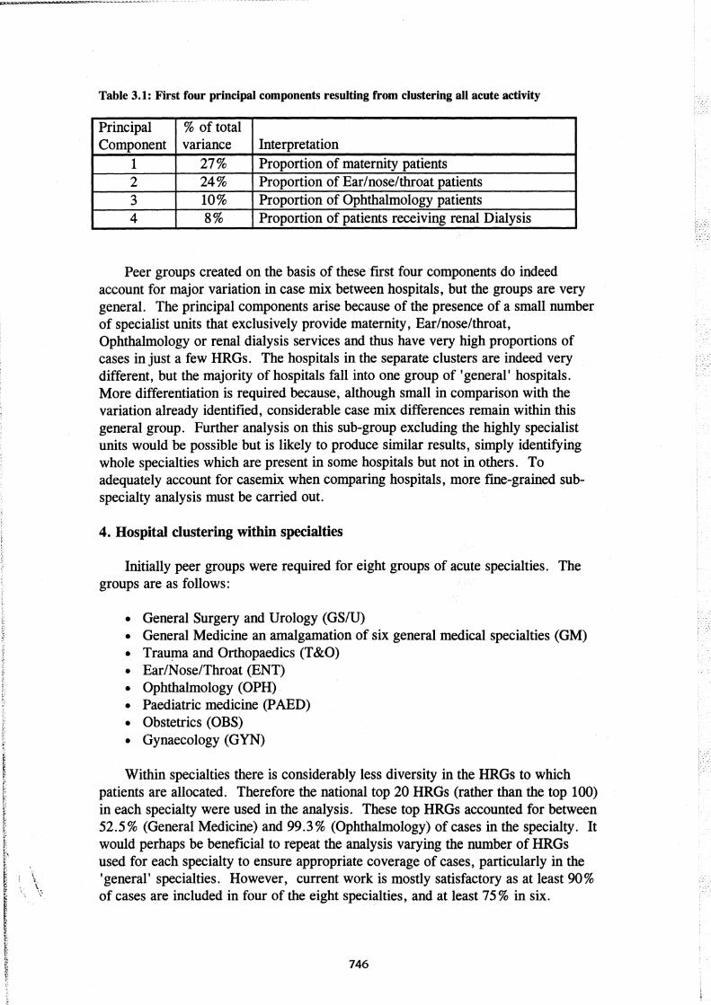
Table 3.1: First four principal components resulting from clustering all acute activity

Principal % of total Component variance Interpretation

1 27% Proportion of maternity patients 2 24% Proportion of Ear/nose/throat patients 3 10% Proportion of Ophthalmology patients 4 8% Proportion of patients receiving renal Dialysis

Peer groups created· on the basis of these first four components do indeed account for major variation in case mix between hospitals, but the groups are very general. The principal components arise because of the presence of a small number of specialist units that exclusively provide maternity, Ear/nose/throat, Ophthalmology or renal dialysis services and thus have very high proportions of cases in just a few HRGs. The hospitals in the separate clusters are indeed very different, but the majority of hospitals fall into one group of 'general' hospitals. More differentiation is required because, although small in comparison with the variation already identified, considerable case mix differences remain within this general group. Further analysis on this sub-group excluding the highly specialist units would be possible but is likely to produce similar results, simply identifying whole specialties which are present in some hospitals but not in others. To adequately account for casemix when comparing hospitals, more fine-grained sub­specialty analysis must be carried out.

4. Hospital clustering within specialties

Initially peer groups were required for eight groups of acute specialties. The groups are as follows:

• General Surgery and Urology (GS/U) • General Medicine an amalgamation of six general medical specialties (GM) • Trau~a and Orthopaedics (T &0) • Ear/Nose/Throat (ENT) • Ophthalmology (OPH) . • Paediatric medicine (PAED) • Obstetrics (OBS) • Gynaecology (GYN)

Within specialties there is considerably less diversity in the HRGs to which patients are allocated. Therefore the national top 20 HRGs (rather than the top 100) in each specialty were used in the analysis. These top HRGs accounted for between 52.5% (General Medicine) and 99.3% (Ophthalmology) of cases in the specialty. It would perhaps be beneficial to repeat the analysis varying the number of HRGs used for each specialty to ensure appropriate coverage of cases, particularly in the 'general' specialties. However, current work is mostly satisfactory as at least 90% of cases are included in four of the eight specialties, and at least 75 % in six.

746

Because proportions of cases in each HRG are being used rather ~ actual numbers, spurious results could arise from low volume specialties, which often have unusual casemix. Therefore hospitals were excluded if they had less than 2000 cases recorded in the specialty.

5. Technical details

Carrying out this analysis using SAS® software is very straightforward. Three procedures are required for the core analysis: the PRINCOMP, CLUSTER and TREE procedures, all of which are part of SAS/ST AT® . These require 9 lines of code. In addition to these, DATA steps and other simple procedures are required, for analysis and graphical display of the resulting clusters.

In performing principal components and cluster analyses, several options are possible. The following significant points should be noted.

• Variables were not standardised before performing PCA (The COV option was used with the PRINCOMP procedure). Standardising would ensure that all variables (i.e. HRG proportions) were given equal weight and this was not desirable here: standardised proportions would be somewhat meaningless.

• The principal component scores output for clustering were standardised (The STANDARD option was used with the PRINCOMP procedure) as it was considered that each component identified was of equal importance. Clustering using unstandardised scores (i.e. scores with variances in proportion to the percentage of total variance explained by the principal component) would result in clusters biased towards the first component and then each subsequen.tcomponent in tum.

• The number of clusters was set to 15 (The NCL= 15 option was set in the TREE procedure).

• Average linkage was used in clustering (The METHOD = AVERAGE option was used in the CLUSTER procedure)

6. Results

6.1 Principal Component Analysis

The principal component analysis indicated that there is indeed a high degree of correlation in proportions of cases between many HRGs; i.e. proportions of cases vary together in many HRGs. In three of the eight specialties just three components account for over 90% of total variance and over 75% in five specialties. Using five components gives at least 75% variance explanation in all specialties. A summary of variance explanation is given in table 6.1

747

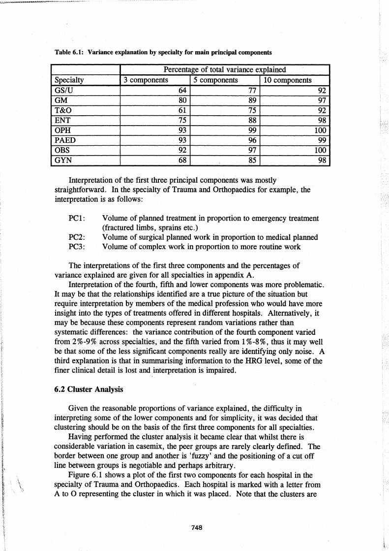
Table 6.1: Variance explanation by specialty for main principal components

Percentage of total variance explained Specialty 3 components 5 components 10 components GS/U 64 77 92 GM 80 89 97 T&O 61 75 92 ENT 75 88 98 OPH 93 99 100 PAED 93 96 99 OBS 92 97 100 GYN 68 85

Interpretation of the first three principal components was mostly straightforward. In the specialty of Trauma and Orthopaedics for example, the interpretation is as follows:

98

PC 1: Volume of planned treatment in proportion to emergency treatment (fractured limbs, sprains etc.)

PC2: Volume of surgical planned work in proportion to medical planned PC3: Volume of complex work in proportion to more routine work

The interpretations of the first three components and the percentages of variance explained are given for all specialties in appendix A.

Interpretation of the fourth, fifth and lower components was more problematic. It may be that the relationships identified are a true picture of the situation but require interpretation by members of the medical profession who would have more insight into the types of treatments offered in different hospitals. Alternatively, it may be because these components represent random variations rather than systematic differences: the variance contribution of the fourth component varied from 2 % -9 % across specialties, and the fifth varied from 1 % -8 %, thus it may well be that some of the less significant components really are identifying only noise. A third explanation is that in summarising information to the HRG level, some of the finer clinical detail is lost and interpretation is impaired.

6.2 Cluster Analysis

Given the reasonable proportions of variance explained, the difficulty in interpreting some of the lower components and for simplicity, it was decided that clustering should be on the basis of the first three components for all specialties.

Having performed the cluster analysis it became clear that whilst there is considerable variation in casemix, the peer groups are rarely clearly defined. The border between one group and another is 'fuzzy' and the positioning of a cut off line between groups is negotiable and perhaps arbitrary.

Figure 6.1 shows a plot of the first two components for each hospital in the specialty of Trauma and Orthopaedics. Each hospital is marked with a letter from A to 0 representing the cluster in which it was placed. Note that the clusters are

748

based on the ftrst three components, . thus not all the information on which they are based is shown here.

It can be seen in ftgure 6.1 that some hospitals have significantly different casemix from the majority. For example,cluster D to the left of the plot contains three hospitals having a very low score on principal component 1. (Le. the proportion of emergency work in these hospitals is very high) and average scores on component2 (Le. the ratio of planned surgical work to planned medical work is around the average). Perhaps these hospitals have large Accident and Emergency departments. Cluster E on the right of the plot represents a very different type of hospital; these have a large proportion of planned activity compared to emergency work, and a somewhat higher ratio of surgical to medical activity within that planned work. In fact, consistent with this description, three of the seven hospitals within this cluster are specialist Orthopaedic units.

It is interesting to note the one hospital in cluster 0 which appears to be comparable with no other unit. Although it has similar scores to the hospitals in cluster E, it differs from these in that it has a very high score on component 3 (indicating a very high complexity workload) which is not shown on the plot. Again, consistent with the description, this hospital specialises in major joint replacement. Clusters K, L M and N also contain only one unit

However, many hospitals fall into a few central, fairly general groups. The peer groups allocated by cluster analysis do contain similar hospitals but the borders appear to be somewhat erratic. In fact, clustering using different linkage methods often results in different clusters, indicating that the method may be a little unstable.

Figure 6.1: Plot of principal component 1 against principal component 2 for each hospital in Trauma and Orthopaedics, showing clusters.

PRIN2 I I

2 + J

I

A AA A AA AA G BJ E

AA AAAAB LAO A AAAAA A AABB BEE

A A AAA AAAAB B E A AAA AAAAAABAA A

o + D F F G A A A A BA E

I

DD FF AAAABAAAB A E E FF F A AAAA AA BBB

M K AAAAAA A I C A A

CC CAA C H C A I

-2 + C C

I

C C C H

H

-4 +

I

N

-6 + I -+--------+--------+--------+--------+--------+--------+--------+--------+ -4 -3 -2 -1 0 1 2 3 4

PRIN1

749

An instance in which clearly·defined clusters do result is paediatric medicine. Figure 6.2 shows the plot of principal components 1 and 3. (Note that the clusters shown are not the same as those shown for Trauma and Orthopaedics.) Here, three general clusters emerge, varying mostly in component 1. This component gives a contrast of the proportion of babies to the proportion of older children. Thus the clusters represent hospitals ranging from those treating mostly babies (positive scores) to those treating mostly older children (negative scores) with a cluster of more general hospitals in between. In fact, many of the hospitals classified here as treating babies are specialist obstetric units and many of those classified as treating older children are specialist paediatric units. There are subdivisions within these three general clusters which represent finer detail, but the general picture is clear.

Figure 6.2. Plot of Principal component 1 against principal component 3 for each hospital in Paediatric Medicine, showing clusters.

PRIN3 I I

4 + I

I 2 +

I I

o +

I -2 +

I I

-4 +

I -6 +

I -8 +

I I

-10 +

I

E EEE E

K

D DDD D

D FF

F F FF F

F F F N

o

G

I I

A AA A A A AAAAAAAAA A AAAA

AAAAAAAA AAA A A G G AAA AAABABBAA B A

GA AAABABABBBBB G G B B ABBBBB B B

B BB B B B

B H

H

C

J C

C CC CC

C C

J

-+-----------+-----------+-----------+-----------+-----------+-----------+ -3 -2 -1 0 1 2 3

PRIN 1

7. Conclusions and Recommendations

The general pattern seen in Trauma and Orthopaedics of some clear, small clusters with a few main general clusters is repeated in most other specialties. Given that the peer groups produced by cluster analysis are arbitrary, it may be sensible to manipulate the groupings after clustering to create more consistent borders. Perhaps cluster analysis should not be used at all; borders could be imposed entirely manually.

750

-.l

_.'l ·"r.

Selection of the top 20 HRGs across all specialties is. perhaps not.desirable. it may be better to select as many HRGs asare required to cover at least 90% of cases for example. Similarly, more principal components could be used in clustering for some specialties to increase the percentage of total variance covered.

The principal components produced and the resulting clusters do seem to be valid when hospitals are matched with the description of the peer groups. Further evaluation and validation would be desirable, but there seems to be considerable potential in the technique.

SAS software is well suited to this analysis: powerful results can be achieved with very little programming and the standard output of the PRINCOMP procedure makes interpretation straightforward.

8. References

Fetter, R.B. (1991). DRGs: Their Design and Development. Health Administration Press, Ann Arbor, Michigan Jeffers, J.N.R. (1967) Two case studies in the application ojprincipal component analysis. Applied Statistics, 16, 225-236 Lautard, D & Jamin, F (1994). Exploitation d'une enquete pour la constitution d'un panel de reseaux. Proceedings of the twelfth SAS® European Users' Group International Conference, Strasbourg. Pearson, K. (1901). On Lines and Planes of Closest Fit to Systems of Points in Space, Philosophical Magazine, 6(2), 559-572.

Contact Address:

Peter Benton Statistician National Casemix Office Highcroft Romsey Rd Winchester, S0225DH England

Tel: +44 1962 844588 Email: peter@wiphm.soton.ac.uk

SAS anct SAS/STAT are registered trademarks of SAS Institute Inc., Cary, NC, USA

751

1.:1

Appendix A: Principal component interpretations and variances explained.

Specialty PC no % Interpretation variance explained

GS/U 1 33 Proportion of General Surgery work relative to Urology

2 17 Unclear: proportion of complex work relative to simple?

3 13 Unclear

GM 1 52 Proportion of renal dialysis 2 21 Proportion of specialist cardiac work 3 9 Proportion of simple investigations (endoscopies)

T&O 1 37 Proportion of planned work relative to trauma 2 14 Proportion of planned surgical work relative to

planned medical 3 10 Proportion of simple work relative to complex

ENT 1 38 Proportion of mouth, nose and throat surgery relative to ear surgery

2 26 Unclear: Proportion of ear/mouth/throat surgery relative to nose surgery?

3 13 Proportion of nose surgery

OPH 1 55 Proportion of major complex work relative to complex

2 33 Proportion of complex work relative to simple 3 6 Unclear

PAED 1 76 Proportion of babies relative to older children 2 15 Unclear: Proportion of rarer work? 3 2 Proportion of 'general paediatrics' relative to

high complexity work OBS 1 46 Proportion of births relative to other obstetric

work 2 37 Unclear (HRG limitation) 3 9 Proportion of mothers relative to babies (poor

coding?*)

GYN 1 43 Proportion of maternity related work relative to other Gynaecology

2 14 Proportion of mothers relative to babies (poor coding*)

3 11 Unclear

* Poor coding: Different hosi?itals have different practices for coding babies. Some give babies a separate record, others do not. Certainly babies should not be coded to Gynaecology but this ~ppears to be happening.

752