identification of planar crack and volumic defects in...
TRANSCRIPT

Identification of planar crack and volumic defects in dynamic viscoelasticity
H.D. BuiEcole Polytechnique, Palaiseau, France
Symposium in the Honor of Professor Leon KeerSymi, July 17-23-2010

I. Dynamic Equations in viscoelasticityII. Usual approaches to some inverse problemsIII. Planar crackIV. Volumic defect (scalar problem)
CONTENTS

I. Dynamic Equations in viscoelasticityII. Usual approaches to some inverse problemsIII. Planar crack (exact solution)IV. Volumic defect (scalar problem)
a) Calderon linearization approachb) Decomposition into two linear problems.c) A numerical method to the source inverse pb.d) The geometry of an inclusion in the scalar and
static case (exact solution)e) The mystery of the Calderon solution
CONTENTS
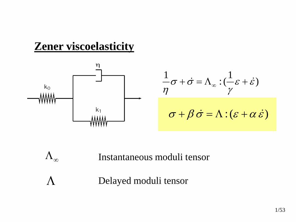
Zener viscoelasticity
1 1: ( )σ σ ε εη γ∞+ = Λ +
Instantaneous moduli tensor
Delayed moduli tensor
: ( )σ β σ ε α ε+ = Λ +
∞Λ
Λ
1/53
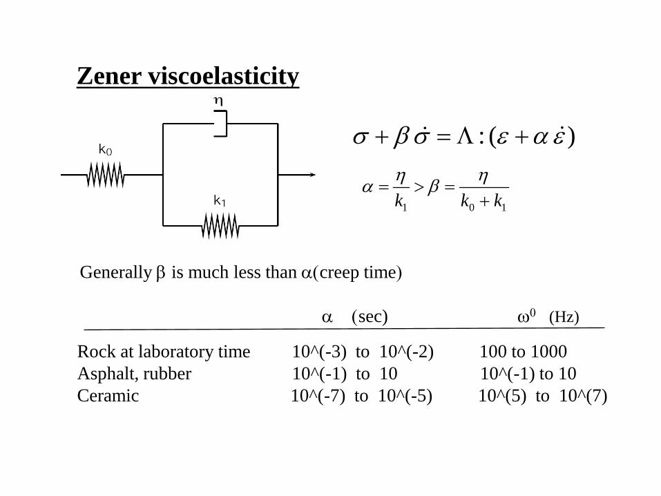
Zener viscoelasticity
: ( )σ β σ ε α ε+ = Λ +
1 0 1k k kη ηα β= > =
+
Generally β is much less than α(creep time)
α (sec) ω0 (Hz)
Rock at laboratory time 10^(-3) to 10^(-2) 100 to 1000Asphalt, rubber 10^(-1) to 10 10^(-1) to 10Ceramic 10^(-7) to 10^(-5) 10^(5) to 10^(7)

Zener viscoelasticity
1 1: ( )σ σ ε εη γ∞+ = Λ +
: ( )σ β σ ε α ε+ = Λ +
* α= +u u uAssociated displacement, strain and stress (Goriacheva, 1973)
*ε ε α ε= +
*σ σ β σ= + * : *σ ε= Λ
1 0 1k k kη ηα β= > =
+
2/53

* α= +u u uAssociated fields (I. Goriacheva, 1973)
*ε ε α ε= +
*σ σ β σ= +
* : *σ ε= Λ
Time harmonic loading
( , ) ( )cost tω=u x v x( , ) ( )cos( )t w tσ ω θ= +x x
Equation of motion
0 and in phase smalldivσ ρ σ θ− = ⇔ ⇒u u
3/53
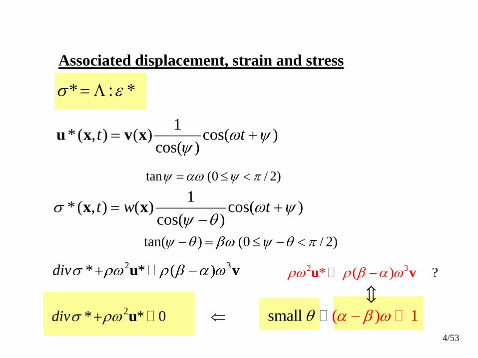
Associated displacement, strain and stress
* : *σ ε= Λ
1*( , ) ( ) cos( )cos( )
t tω ψψ
= +u x v x
tan (0 / 2)ψ αω ψ π= ≤ <
1*( , ) ( ) cos( )cos( )
t w tσ ω ψψ θ
= +−
x x
tan( ) (0 / 2)ψ θ βω ψ θ π− = ≤ − <
2 3* * ( )divσ ρω ρ β α ω+ −u v
2* * 0divσ ρω+ ⇐u (mall ) 1s α β ωθ −
2 3* ?( )ρω ρ β α ω−u v
4/53
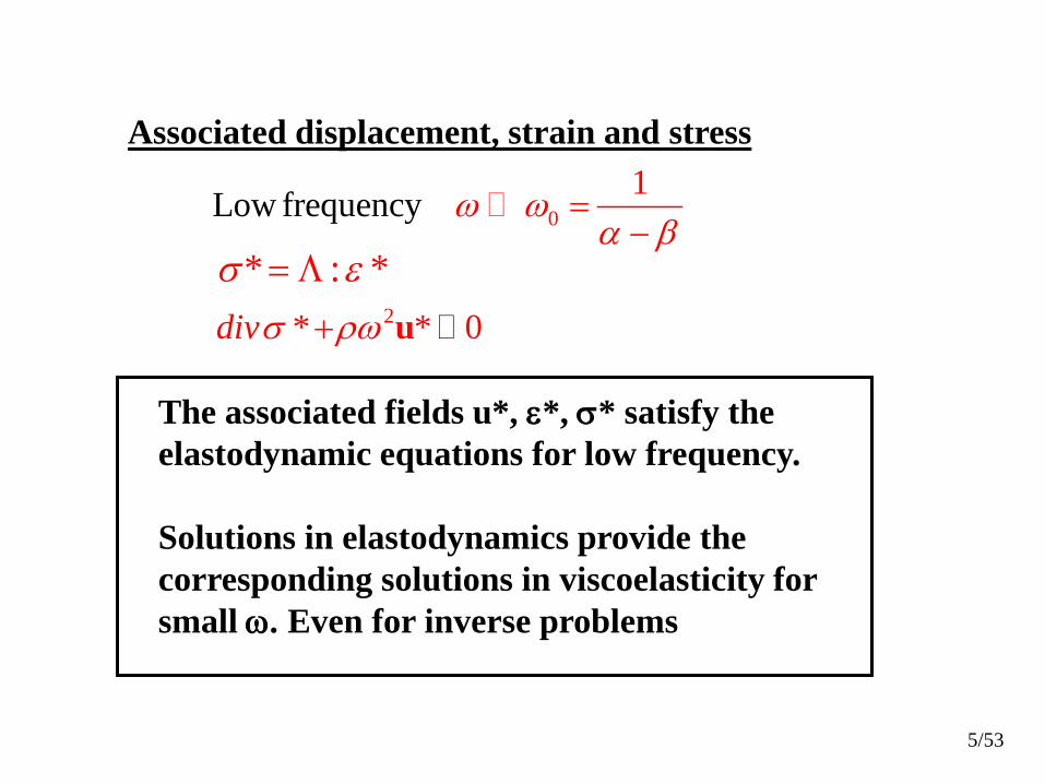
Associated displacement, strain and stress
* : *σ ε= Λ2* * 0divσ ρω+ u
0Low frequency 1ω ωα β
=−
The associated fields u*, ε*, σ* satisfy the elastodynamic equations for low frequency.
Solutions in elastodynamics provide the corresponding solutions in viscoelasticity for small ω. Even for inverse problems
5/53
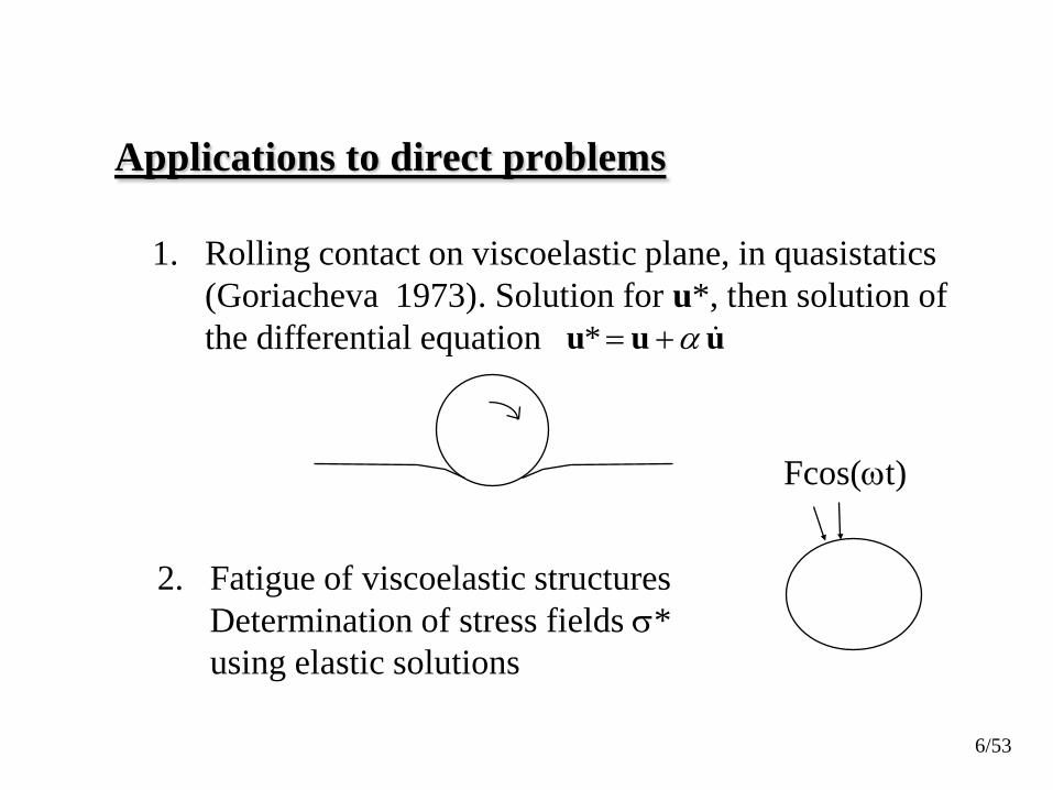
Applications to direct problems
1. Rolling contact on viscoelastic plane, in quasistatics(Goriacheva 1973). Solution for u*, then solution ofthe differential equation
2. Fatigue of viscoelastic structuresDetermination of stress fields σ*using elastic solutions
* α= +u u u
Fcos(ωt)
6/53
Applications to inverse problems
1. Identification of a planar crack in a 3D bounded solid from surface data u* and T*
2. Identification of a defect (tumor, damaged zone)in a bounded solid from surface data u* and T*
7/53

• General approach to Inverse problems in Viscoelasticity with relaxation functions
0 0( ) ( ) ( ) 2 ( ) ( )
t t
ij ij kk ijt t d t dσ λ τ δ ε τ τ µ τ ε τ τ= − + −∫ ∫
F
Loading Ti(t)
Dynamic Response ui(t)
• Find the crack F under dynamic loadings from surface data measurements
8/53
• General method of solution• Optimization in a four-dimensional space ! • R3×[0,T] for the static or dynamic case
9/53

2( ) ( )S
F T Arg Mi u Sn u= −
2 2
0( ) ( , ) ( )
Tu dA u tu S dS u t t
∂Ω− = −∫ ∫Ti(t) ⇒ u(t, S) ⇒
F
Loading Ti(t)
Response ui(t)
S
Optimization or Control theory in 4
Very ill-posed problems
2( )S
SMin u u−Minimize the residual
10/53

2( ) ( )S
F t Arg Mi u Sn u= −
Control theory in for elastodynamics 4
(Das and Suhadolc, 1996) Oxford University
"even if the fitting of data seems to be quite good, the faulting process is poorly reproduced, so that in the real case, it would be difficult to know when one has obtained the correct solution”.
Earthquake inverse problems to determine the fault process (moving fault F(t))
11/53

Inverse crack problem of the real vectorial Helmholtz equation
Load TdResponse ud
(We only consider a stationary planar crack)
Bui et al, Annals of Solid and Structural Mech (2010)12/53

Inverse crack problem of the real vectorial Helmholtz equation
The approach is originated from Calderon’s method (1980) for determining an inclusion in the harmonic case,
then extended to crack problems in elasticity (Andrieux et al, 1999),to transient elastodynamics (Bui et al, 2005), with applicationsto the earthquake inverse problem (Bui, 2006),to the scalar Helmholtz equation (Ben Abda et al, 2005) andto the vectorial Helmholtz equation (Bui et al, 2010)
The method used is based on the reciprocity gap functional13/53

Inverse crack problem of the real scalar Helmholtz equation in 3D
(Ben Abda et al, 2005)
k=40
k=25
k=15
Exact Reconstructed (no noise)
14/53

Inverse crack problem of the real scalar Helmholtz equation
(Ben Abda et al, 2005)
k=40
No noise Reconstructedwith 5% noise on data
15/57

The nonlinear variational equation for a crack in 3D elasticity
Find F such that the displacement discontinuity [u] satisfies
[ ] ( **( ) ( ) ( )) *extSF
dS dSσ σ σ= −∫ ∫ uu . w .n w. . w .n.n uF
∀ w ( Adjoint field satisfying the Helmholtz in Ω)
div grad u* +ρω2 u* =0 in Ω\F( *) on Fσ =u .n 0
R, linear in w is called reciprocity gap functional ( *)( ) ( )*
extSR dSσσ −∫ u .n uw w. . w .n
div grad w +ρω2 w* =0 in ΩNo boundary condition
16/53

1.The non linear variational equation
Find F such that:
[ ]*( ) ( ) *, *( ; )F
d RF Sσ =∫ u . w .n T uw
∀ w ( Adjoint field satisfying the Helmholtz in Ω)
*,( ; ) ( )(* *) *extS
R dSσ σ−∫ u .w w. n u . w .nT u
We take advantage of the arbitrariness of adjoint functionsto parameterize w by a set of parameters p ⇒ R(p), with dimp=dimunknowns
17/53

1.The non linear variational equation
Find F such that:
[ ]*( ) ( ) *, *( ; )F
d RF Sσ =∫ u . w .n T uw
∀ w ( Adjoint field satisfying the Helmholtz in Ω)
If [u*]=0 : R=0 (Reciprocity theorem) No defectR≠0 is a defect indicator.
The crack identification consists in searching the zerosof R(p), with dimp=dimunknowns.It is a Zero crossing method.
18/53
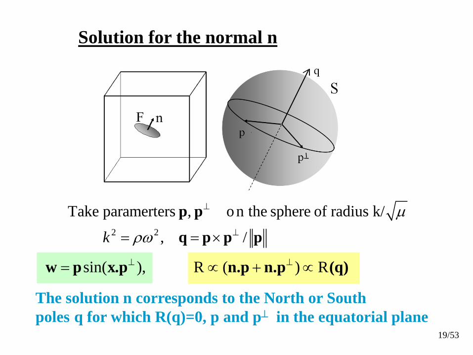
Solution for the normal n
Take paramerters , o n the sphere of radius k/ µ⊥p p2 2 , /k ρω ⊥= = ×q p p p
The solution n corresponds to the North or South poles q for which R(q)=0, p and p⊥ in the equatorial plane
sin( ), R ( ) R⊥ ⊥= ∝ + ∝w p x.p n.p n.p (q)
19/53
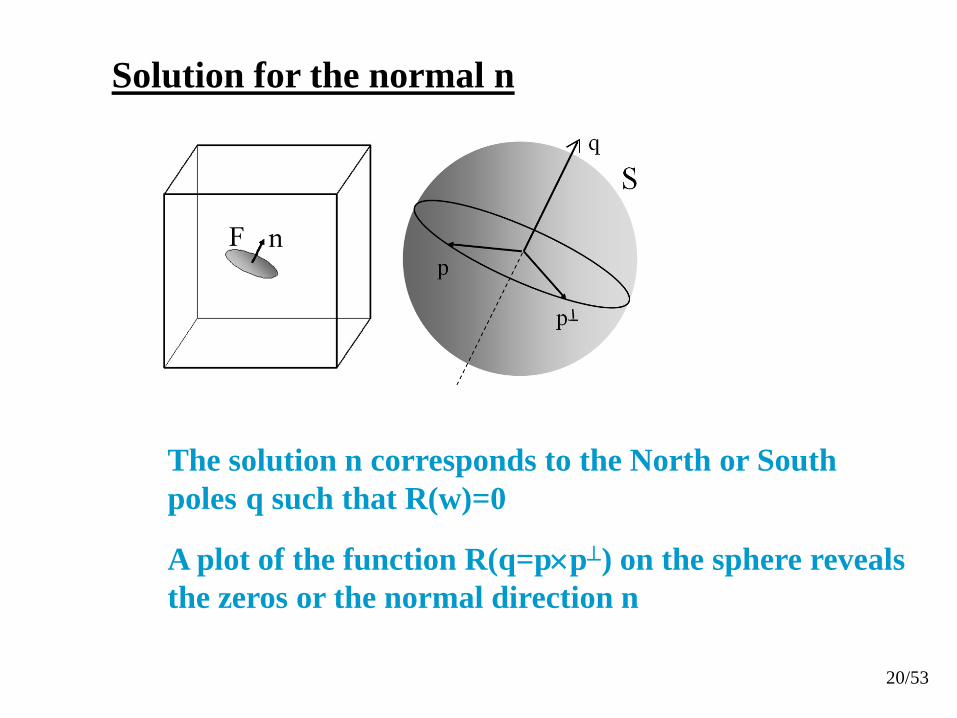
Solution for the normal n
The solution n corresponds to the North or South poles q such that R(w)=0
A plot of the function R(q=p×p⊥) on the sphere reveals the zeros or the normal direction n
20/53

Solution for the crack plane x3−D=0
D
x3
2kq
λ µ=
+3
3( ) cos( ( )) ( ) sin( ( ))q x R q Dκ κ κ κ= − ⇒ ∝ −w e
2choose k or q such that Lqπ
>
L
We find that D is the unique zero R(κ=D)=0
21/53
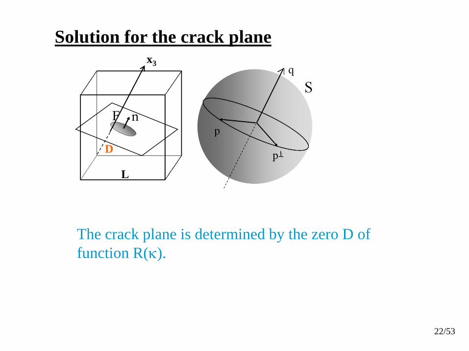
Solution for the crack plane
D
x3
L
The crack plane is determined by the zero D offunction R(κ).
22/53
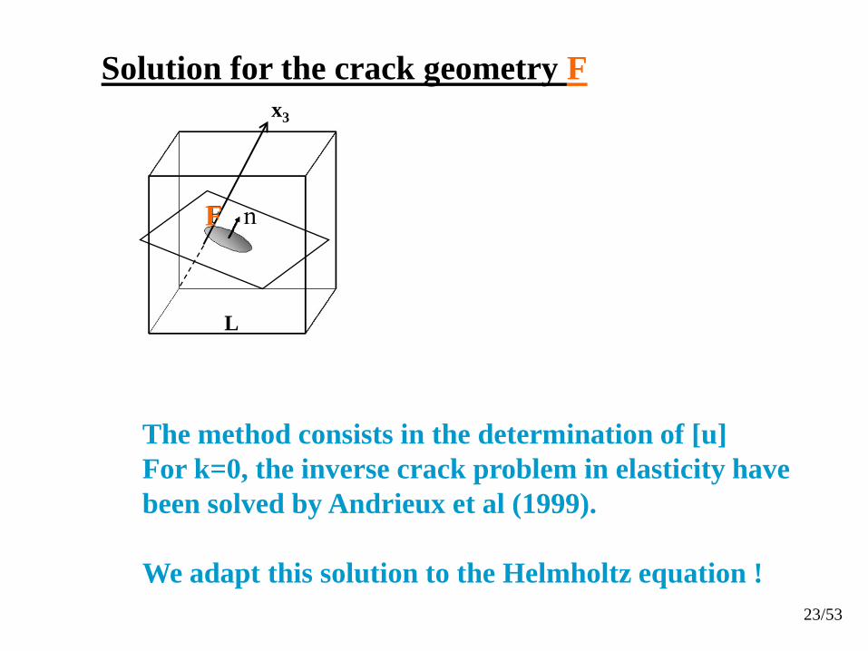
Solution for the crack geometry F
F
x3
L
The method consists in the determination of [u]For k=0, the inverse crack problem in elasticity have been solved by Andrieux et al (1999).
We adapt this solution to the Helmholtz equation !23/53
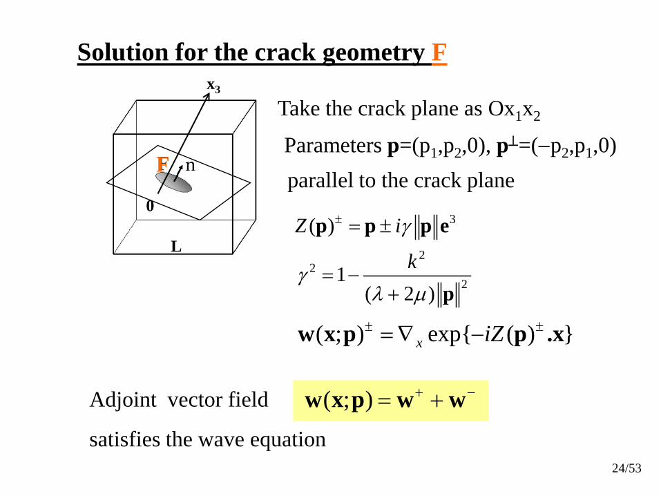
Solution for the crack geometry F
F
x3
L
0
Take the crack plane as Ox1x2
Parameters p=(p1,p2,0), p⊥=(−p2,p1,0)
3( )Z iγ± = ±p p p e2
221
( 2 )kγ
λ µ= −
+ p
( ; ) + −= +w x p w w
( ; ) exp ( ) x iZ± ±= ∇ −w x p p .x
Adjoint vector field
satisfies the wave equation
parallel to the crack plane
24/53

Solution for the crack geometry F
F
x3
L
0
Take the crack plane as Ox1x2
3( )Z iγ± = ±p p p e2
221
( 2 )kγ
λ µ= −
+ p
( ; ) ,+ −= +w x p w w( ; ) exp ( ) ,x iZ± ±= ∇ −w x p p .x
[ ] 3
1 23 2 22 20
exp( ) ( ; )1( )(2 ) 2 ( 1)
,2p
d di R dp dpuπ λ γ µγ=
=− +∫
u Tp.x pxp
Parameters p=(p1,p2,0), p⊥=(−p2,p1,0)parallel to the crack plane
25/53
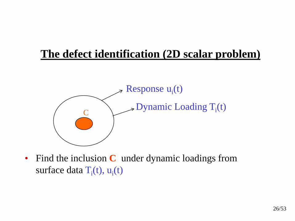
C
Response ui(t)
Dynamic Loading Ti(t)
• Find the inclusion C under dynamic loadings from surface data Ti(t), ui(t)
The defect identification (2D scalar problem)
26/53

The 2D scalar problem
2( )(1 ) *( ; ) * 0div grad u x kh uh+ + =x
By linearization
* gun∂
=∂
*u f=
in Ω
Data on ∂Ω
Calderon (1980) solved the inverse problem for small value of h(x) and (statics)0k =
27/53

The 2D scalar problem
2( )(1 ) *( ; ) * 0div grad u x kh uh+ + =x
Calderon’s linearization (1980) in the static case k=0,for small h, upon replacing grad u*(x,h) by grad u*(x,0)
* gun∂
=∂
*u f=
in Ω
on ∂Ω
The linearized solution for k≠0 is straightforwards
Normalized shear modulus, perturbation h(x)
30/53

The nonlinear case
2(( ; ) ( ; , ),( ) )xgrad u x grad d x gh Rh f ϕϕϕ = ∀∫Cx
2 0 indiv grad kϕ ϕ+ = Ω
Nonlinear variational equation for h and C
Find h(x) (we drop the * symbol)
( ; ) ( ),R dsf g g fnϕϕ ϕ
∂Ω
∂= −
∂∫ (Data linear form in ϕ)
31/53

Reduction to two linear problems
( ) ( ; )U x u x h=
2 0 in( )div grad u k Su+ + = Ωx
( ) ( ) ( ; )div gr had uS h= xx x
Problem I (source inverse problem): Solution denoted by U(x)
+ The same two boundary data f, g and
♦
♦ Problem II
where is the solution of Problem I
2((1 ) ( ; )) 0div gra u uhdh x k+ + =x
2
( )( ) ,;( ( ) )) (
Supp Sh gradU grad d x R f g ϕϕϕ = ∀∫ xx x
32/53

( ) : ( ; )U x u x h=
2 0 in( )div grad u k Su+ + = Ωx
( ) ( ) ( ; )div gr had uS h= xx x
Problem I (source inverse problem): Solution U(x)
+ The same two boundary data
♦
The solution of problem I provides the source S(x) and
33/53

( ) : * ( ; )U x u x h=
2 * * 0( ) indiv grad u Su k+ + = Ωx
( ) ( ) *( ; )div gr hd uS h a= xx x
Problem I (source inverse problem): Solution U(x)
+ The same two boundary data
♦
The solution of problem I provides the source S(x) and
The support of function S(x) is the same of supp(h) i.e. the geometry of the inclusion is determined by a source inverse problem
34/53

( ) : ( ; )U x u x h=
2 0 in( )div grad u k Su+ + = Ωx
( ) ( ) ( ; )div gr had uS h= xx x
Problem I (source inverse problem): Solution U(x)
+ The same two boundary data
♦
The solution of problem I provides the source S(x) and
The support of function S(x) is the same of supp(h) i.e. the geometry of the inclusion is determined by a source inverse problemSource inverse problem is solved by Alves and Ha Duong (1997)
35/53

( ) ( ; )U x u x h=
( )
2( ) ( )( ( ; ,)) ;Supp S
gradU grad d x Rh gfϕϕ ϕ= ∀∫ xx xξ♦ Problem II
where is the solution of Problem I
Since C=supp(S)
Problem II provides a linear Volterra integral eq. for h(x)with kernel Thus the nonlinear Calderon’s inverse problem reduces to two linear problems !
( ( ; ))gradU grad ϕ xξx
( ; )ϕ xξ is the adjoint field depending on parameter ξ 2∈
36/53
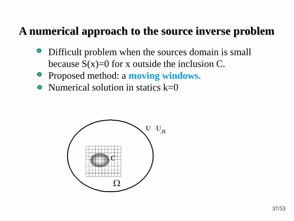
A numerical approach to the source inverse problem
Difficult problem when the sources domain is smallbecause S(x)=0 for x outside the inclusion C.Proposed method: a moving windows.Numerical solution in statics k=0
37/53

G
Bad window G : wrong solution
Window
38/53
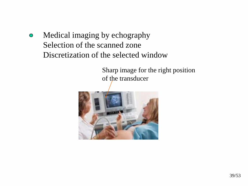
Medical imaging by echographySelection of the scanned zoneDiscretization of the selected window
Sharp image for the right position of the transducer
39/53

Detection of a tumor Discretization of a selected windows
40/53

Detection of a tumor Discretization of a selected windows
41/53

Detection of a tumor Bad windows, wrong solution, blurred image
42/53

Detection of a tumor Bad windows, wrong solution, blurred image
2
2
2
( ) : large error
( ) : small error "Good" solution
( ) 0 Exact solution
Wrong solutionZ
Z
Z
Min u Z
Min u Z
u
n
u
uMi u Z
− ⇒
− ⇒
− = ⇒
43/53

Detection of a tumor Bad windows, wrong solution, blurred image
44/53

Detection of a tumor Correct windows, good/exact solution, Sharper image
45/53

Detection of a tumor Correct windows, good/exact solution, Sharper image
46/53
CONCLUSIONS
♦
♦
The Zener viscoelasticity law enables us to establishan elastic-viscoelastic correspondence for low frequency
The use of Goriacheva’s associated fields leads to the dynamic equation in elasticity for low ω
Inverse problems in viscoelasticity to determine a planar crack and a volumic defectare solved by the reciprocity gap functional method.
♦
53/53

Congratulations to Leon Keer
Thank you
and

2 ( ) 0) i( ndiv gradU x k U S+ + = Ωx
Problem I (source inverse problem)
and are known onuun
∂∂Ω
∂Solution given by Alves and Ha Duong (1997)for N point sources
If S(x) is a finite sum of point sources Si of intensity qi the solution exists and is unique.

Discretize the expected windows containing C
1( ) ( )
N
i ii
qS δ=
= −∑ ax x 2N unknowns ai, qi
Non linear systems of equations obtained with 2N adjoint fields