crack width measurement for non-planar surfaces by ...€¦ · crack width measurement for...

CRACK WIDTH MEASUREMENT FOR NON-PLANAR SURFACES BY TRIANGLEMESH ANALYSIS IN CIVIL ENGINEERING MATERIAL TESTING

F. Liebold1, H.-G. Maas1, A. A. Heravi2

1 Institute of Photogrammetry and Remote Sensing, Technische Universitat Dresden, Germany -(frank.liebold, hans-gerd.maas)@tu-dresden.de

2 Institute of Construction Materials, Technische Universitat Dresden, Germany - [email protected]

Commission II

KEY WORDS: Material Testing, Deformation Measurement, Crack Width Measurement, Triangle Mesh, Non-planar Surface

ABSTRACT:

This publication concentrates on the photogrammetric crack width measurement of crack patterns of concrete probes under impactloading in high-speed stereo image sequences. The presented algorithm works for non-planar specimens with deformations that onlyappear tangential to the surface and the method is based on triangle mesh analysis. Experiments were conducted with cylindricalspecimens with an impact load affecting parallel to the main axis of the cylinder.

1. INTRODUCTION

To reduce damage from impact loading due to natural catastro-phes, buildings and walls can be strengthened with material-bonded composites. These composites are analyzed in dynamictests where photogrammetric deformation measurement tech-niques are used. High-speed stereo systems offer the possibilityto analyze impact tests due to their high temporal resolution.For civil engineers, the detection of cracks and the measure-ment of the according widths are an interesting issue. In recentyears, several publications were contributed in the field of pho-togrammetric crack width determination. (Dare et al., 2002)applied edge detection techniques such as the Fly-Fisher algo-rithm and the Route-Finder algorithm to detect cracks in singleimages of crack patterns and also measured crack widths bythe analysis of profiles perpendicular to the crack courses. In(Lange, Benning, 2006), the theoretical crack opening vector isexpressed as follows:

~tc =

crack widthcrack edge displacement along the crack course

vertical crack edge displacement

(1)

where ~tc = crack opening vector

This vector bases on the theoretical modes of fracture referingto (Irwin, 1958). (Lange, Benning, 2006) measured artificialtargets on concrete specimens with a multi-ocular camera sys-tem and computed crack widths with a method given by (Gortz,2004) using averages of displacements in 4-point-elements, alsoincluding the direction of the cracks. However, global rotationsbetween the epochs were neglected. (Barazzetti, Scaioni, 2009)presented a 2D image sequence analysis procedure to deter-mine crack deformations using artificial targets and an orien-tation frame. (Maas, Hampel, 2006) and (Hampel, Maas, 2009)used digital image correlation techniques to compute a densedisplacement field and to analyze crack openings in horizon-tal and vertical profiles. (Liebold, Maas, 2018) show how tocompute crack widths of concrete probes in monocular imagesequences using triangle mesh analysis.

Monocular image sequences can only be used for planar sur-faces and if the deformations only appear in this plane. Theapproach presented in this publication gives an extension tothe work of (Liebold, Maas, 2018). It will be shown how todetect deformations on non-planar surfaces in triangle meshesbetween two epochs. Herein, the triangles are transformed into2D space using the parametrization of a known surface and areanalyzed with the 2D algorithm of (Liebold, Maas, 2018). Astereo system is used to measure 3D surface points for eachepoch of the sequence. With the mesh analysis of 3D surfacepoints, it is possible to work with non-planar surfaces, for ex-ample, from cylindrical specimen. Another advantage of stereosystems is the robustness against relative movements betweenthe object and the camera system. A prerequisite for the algo-rithm presented here are deformations that are only tangential tothe surface (only opening and in-plane shear). Our experimentsare designed such that this condition is fulfilled. It is assumedthat there is no out-of-plane shear, what means that the z com-ponent in Eq. 1 is zero.

The next chapter deals with the description of the experimentalsetup. In the following part, the method for the crack widthdetermination is presented. After this, the application in theexperiment is shown. At the end, a conclusion and an outlookis given.

2. EXPERIMENTAL SETUP

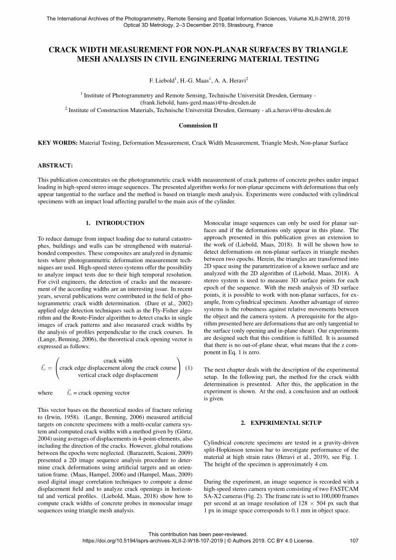
Cylindrical concrete specimens are tested in a gravity-drivensplit-Hopkinson tension bar to investigate performance of thematerial at high strain rates (Heravi et al., 2019), see Fig. 1.The height of the specimen is approximately 4 cm.

During the experiment, an image sequence is recorded with ahigh-speed stereo camera system consisting of two FASTCAMSA-X2 cameras (Fig. 2). The frame rate is set to 100,000 framesper second at an image resolution of 128 × 504 px such that1 px in image space corresponds to 0.1 mm in object space.

The International Archives of the Photogrammetry, Remote Sensing and Spatial Information Sciences, Volume XLII-2/W18, 2019 Optical 3D Metrology, 2–3 December 2019, Strasbourg, France

This contribution has been peer-reviewed. https://doi.org/10.5194/isprs-archives-XLII-2-W18-107-2019 | © Authors 2019. CC BY 4.0 License.

107

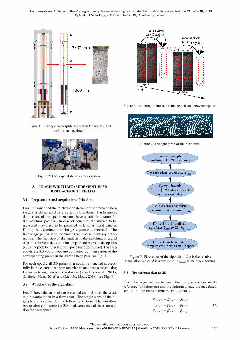
Figure 1. Gravity-driven split-Hopkinson tension bar andcylindrical specimen.

Figure 2. High-speed stereo camera system.

3. CRACK WIDTH MEASUREMENT IN 3DDISPLACEMENT FIELDS

3.1 Preparation and acquisition of the data

First, the inner and the relative orientation of the stereo camerasystem is determined in a system calibration. Furthermore,the surface of the specimen must have a suitable texture forthe matching process. In case of concrete, the surface to bemeasured may have to be prepared with an artificial pattern.During the experiment, an image sequence is recorded. Thefirst image pair is acquired under zero load without any defor-mation. The first step of the analysis is the matching of a gridof points between the stereo image pair and between the epochs(current epoch to the reference epoch under zero load). For eachepoch, the 3D coordinates are computed by intersection of thecorresponding points in the stereo image pair, see Fig. 3.

For each epoch, all 3D points that could be matched success-fully in the current time step are triangulated into a mesh usingDelaunay triangulation as it is done in (Koschitzki et al., 2011),(Liebold, Maas, 2016) and (Liebold, Maas, 2018), see Fig. 4.

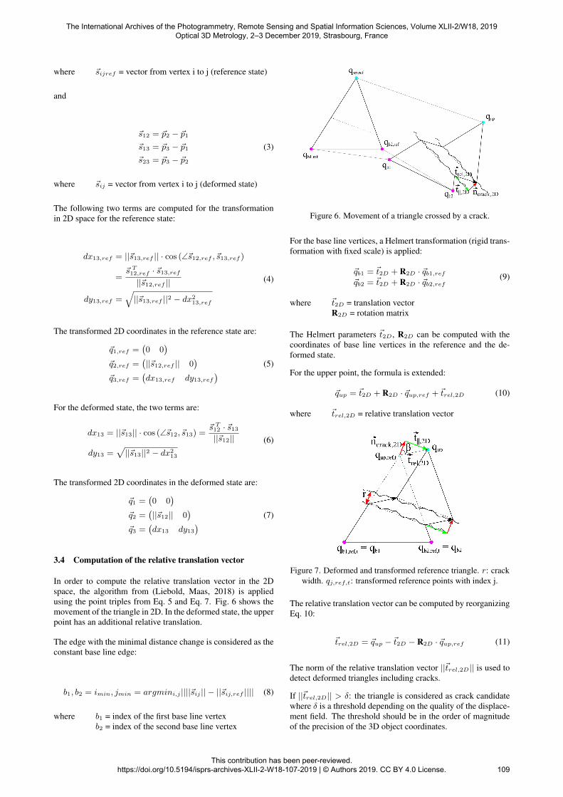
3.2 Workflow of the algorithm

Fig. 5 shows the steps of the presented algorithm for the crackwidth computation in a flow chart. The single steps of the al-gorithm are explained in the following sections. The workflowbegins after computing the 3D displacements and the triangula-tion for each epoch.

Figure 3. Matching in the stereo image pair and between epochs.

Figure 4. Triangle mesh of the 3D points.

Figure 5. Flow chart of the algorithm: ~trel is the relativetranslation vector. δ is a threshold. ~ncrack is the crack normal.

3.3 Transformation to 2D

First, the edge vectors between the triangle vertices in thereference (undeformed) and the deformed state are calculated,see Eq. 2. The triangle indices are 1, 2 and 3.

~s12ref = ~p2ref − ~p1ref~s13ref = ~p3ref − ~p1ref~s23ref = ~p3ref − ~p2ref

(2)



108

where ~sijref = vector from vertex i to j (reference state)

and

~s12 = ~p2 − ~p1~s13 = ~p3 − ~p1~s23 = ~p3 − ~p2

(3)

where ~sij = vector from vertex i to j (deformed state)

The following two terms are computed for the transformationin 2D space for the reference state:

dx13,ref = ||~s13,ref || · cos (∠~s12,ref , ~s13,ref )

=~s T12,ref · ~s13,ref||~s12,ref ||

dy13,ref =√||~s13,ref ||2 − dx213,ref

(4)

The transformed 2D coordinates in the reference state are:

~q1,ref =(0 0

)~q2,ref =

(||~s12,ref || 0

)~q3,ref =

(dx13,ref dy13,ref

) (5)

For the deformed state, the two terms are:

dx13 = ||~s13|| · cos (∠~s12, ~s13) =~s T12 · ~s13||~s12||

dy13 =√||~s13||2 − dx213

(6)

The transformed 2D coordinates in the deformed state are:

~q1 =(0 0

)~q2 =

(||~s12|| 0

)~q3 =

(dx13 dy13

) (7)

3.4 Computation of the relative translation vector

In order to compute the relative translation vector in the 2Dspace, the algorithm from (Liebold, Maas, 2018) is appliedusing the point triples from Eq. 5 and Eq. 7. Fig. 6 shows themovement of the triangle in 2D. In the deformed state, the upperpoint has an additional relative translation.

The edge with the minimal distance change is considered as theconstant base line edge:

b1, b2 = imin, jmin = argmini,j ||||~sij || − ||~sij,ref |||| (8)

where b1 = index of the first base line vertexb2 = index of the second base line vertex

Figure 6. Movement of a triangle crossed by a crack.

For the base line vertices, a Helmert transformation (rigid trans-formation with fixed scale) is applied:

~qb1 = ~t2D + R2D · ~qb1,ref~qb2 = ~t2D + R2D · ~qb2,ref

(9)

where ~t2D = translation vectorR2D = rotation matrix

The Helmert parameters ~t2D, R2D can be computed with thecoordinates of base line vertices in the reference and the de-formed state.

For the upper point, the formula is extended:

~qup = ~t2D + R2D · ~qup,ref + ~trel,2D (10)

where ~trel,2D = relative translation vector

Figure 7. Deformed and transformed reference triangle. r: crackwidth. qj,ref,t: transformed reference points with index j.

The relative translation vector can be computed by reorganizingEq. 10:

~trel,2D = ~qup − ~t2D − R2D · ~qup,ref (11)

The norm of the relative translation vector ||~trel,2D|| is used todetect deformed triangles including cracks.

If ||~trel,2D|| > δ: the triangle is considered as crack candidatewhere δ is a threshold depending on the quality of the displace-ment field. The threshold should be in the order of magnitudeof the precision of the 3D object coordinates.



109

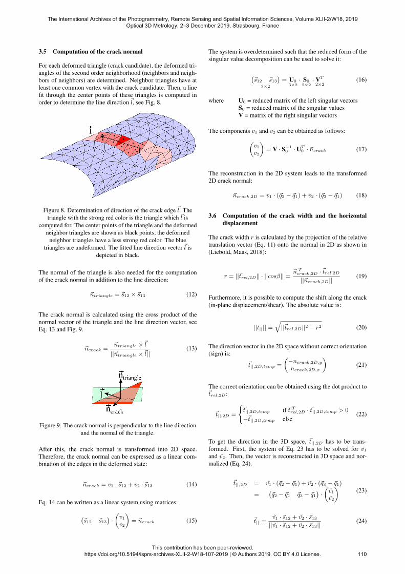
3.5 Computation of the crack normal

For each deformed triangle (crack candidate), the deformed tri-angles of the second order neighborhood (neighbors and neigh-bors of neighbors) are determined. Neighbor triangles have atleast one common vertex with the crack candidate. Then, a linefit through the center points of these triangles is computed inorder to determine the line direction ~l, see Fig. 8.

Figure 8. Determination of direction of the crack edge ~l. Thetriangle with the strong red color is the triangle which ~l is

computed for. The center points of the triangle and the deformedneighbor triangles are shown as black points, the deformed

neighbor triangles have a less strong red color. The bluetriangles are undeformed. The fitted line direction vector ~l is

depicted in black.

The normal of the triangle is also needed for the computationof the crack normal in addition to the line direction:

~ntriangle = ~s12 × ~s13 (12)

The crack normal is calculated using the cross product of thenormal vector of the triangle and the line direction vector, seeEq. 13 and Fig. 9.

~ncrack =~ntriangle ×~l||~ntriangle ×~l||

(13)

Figure 9. The crack normal is perpendicular to the line directionand the normal of the triangle.

After this, the crack normal is transformed into 2D space.Therefore, the crack normal can be expressed as a linear com-bination of the edges in the deformed state:

~ncrack = v1 · ~s12 + v2 · ~s13 (14)

Eq. 14 can be written as a linear system using matrices:

(~s12 ~s13

)·(v1v2

)= ~ncrack (15)

The system is overdetermined such that the reduced form of thesingular value decomposition can be used to solve it:

(~s12 ~s13

)3×2

= U03×2· S02×2· VT

2×2(16)

where U0 = reduced matrix of the left singular vectorsS0 = reduced matrix of the singular valuesV = matrix of the right singular vectors

The components v1 and v2 can be obtained as follows:(v1v2

)= V · S−1

0 · UT0 · ~ncrack (17)

The reconstruction in the 2D system leads to the transformed2D crack normal:

~ncrack,2D = v1 · (~q2 − ~q1) + v2 · (~q3 − ~q1) (18)

3.6 Computation of the crack width and the horizontaldisplacement

The crack width r is calculated by the projection of the relativetranslation vector (Eq. 11) onto the normal in 2D as shown in(Liebold, Maas, 2018):

r = ||~trel,2D|| · ||cosβ|| =~n Tcrack,2D · ~trel,2D||~ncrack,2D||

(19)

Furthermore, it is possible to compute the shift along the crack(in-plane displacement/shear). The absolute value is:

||t|||| =√||~trel,2D||2 − r2 (20)

The direction vector in the 2D space without correct orientation(sign) is:

~t||,2D,temp =

(−ncrack,2D,y

ncrack,2D,x

)(21)

The correct orientation can be obtained using the dot product to~trel,2D:

~t||,2D =

{~t||,2D,temp if ~t T

rel,2D · ~t||,2D,temp > 0

−~t||,2D,temp else(22)

To get the direction in the 3D space, ~t||,2D has to be trans-formed. First, the system of Eq. 23 has to be solved for v1and v2. Then, the vector is reconstructed in 3D space and nor-malized (Eq. 24).

~t||,2D = v1 · (~q2 − ~q1) + v2 · (~q3 − ~q1)

=(~q2 − ~q1 ~q3 − ~q1

)·(v1v2

)(23)

~t|| =v1 · ~s12 + v2 · ~s13||v1 · ~s12 + v2 · ~s13||

(24)



110

4. APPLICATION OF THE CRACK WIDTHDETERMINATION IN THE EXPERIMENT

4.1 Computation of the 3D displacements

The system calibration and the computation of the 3D displace-ments are done with the commercial software ARAMIS devel-oped by GOM GmbH. The 3D coordinates and displacementsserve as input for the application of the crack detection andcrack width computation.

4.2 Crack detection and crack width analysis

The algorithm from section 3 is applied on the data. δ is set to0.02 mm (corresponds to 0.2 px in image space) and defines thethreshold for crack candidates.

Fig. 10 shows color-coded maps of the norms of the relativetranslations of the triangles for the first time steps where defor-mations could be detected. Therefore, the color-code is verysensitive. The widths are changing in the sequence. After0.19 ms, the first cracks appear in the visualization. On the farleft, there is an area where it is not sure if there is a crack. Later,this possible crack closes as other cracks open. The largestcrack at time step of 0.20 ms closes in the following time stepstoo, whereas the neighbor cracks become larger.

Figure 10. Crack detection. Visualization of ||~trel,2D|| for eachtriangle for some selected time steps at the begin of the crack

opening.

Triangles with ||~trel,2D|| > δ can be merged to a region if thereare neighbors that also fulfill this condition using region grow-ing, see Fig. 11.

Fig. 12 and Fig. 13 show color-coded visualizations of thenorms of the relative translation vectors ||~trel,2D|| for two laterepochs with 2 cracks. In addition, the histograms of the crackwidths of the two crack areas are depicted. In these histograms,some statistical values are given: the mean of the crack widthsr, the median rmedian, the maximum crack width rmax, the

Figure 11. Color-labeled regions of triangles with ||~trel,2D|| > δat 0.22 ms.

standard deviation of the crack widths σr and the standard de-viation σr,MAD computed using the median absolute deviation(MAD) which is more robust against outliers.

σr,mad = k ·median

||r1 −median(~r)||||r2 −median(~r)||

...

withk = q−1

0.75 ≈ 1.48

(25)

where σr,mad = standard deviation computed with MAD~r = vector with the measured crack widthsqp = quantile of order p for N (0, 1)N (0, 1) = standard normal distribution

Figure 12. Color-coded visualization of ||~trel,2D|| for epoch 25at 0.24 ms. For the two cracks, histograms of the crack widthsare depicted. In addition, the original image of one camera is

shown.

In the histograms, some outliers appear due to uncertainties inthe normal vector computation at the borders of the mesh. An-other reason for outliers are incorrect matching results that areinfluenced by cracks crossing matching patches. Therefore, inthe neighborhood of crack triangles, there are some trianglesthat are also detected as crack candidates (||~trel,2D|| > δ) buthave smaller values of ||~trel,2D||.

The diagram in Fig. 14 shows 4 curves: the sum of the meancrack widths of the crack areas (

∑rmean), the sum of medi-

ans (∑rmedian) and the sum of the maxima (

∑rmax). In

addition, the total deformation of the sample that is calcu-lated with the wave analysis in the split-Hopkinson tensionbar is depicted (

∑rwaveanalysis) to compare the crack widths

with another measurement method. The values of mean andmedian are strongly depending on the threshold δ which isset to 0.02 mm in this experiment because δ defines which



111

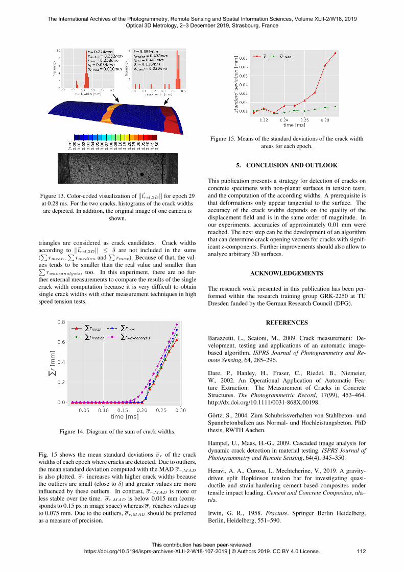
Figure 13. Color-coded visualization of ||~trel,2D|| for epoch 29at 0.28 ms. For the two cracks, histograms of the crack widthsare depicted. In addition, the original image of one camera is

shown.

triangles are considered as crack candidates. Crack widthsaccording to ||~trel,2D|| ≤ δ are not included in the sums(∑rmean,

∑rmedian and

∑rmax). Because of that, the val-

ues tends to be smaller than the real value and smaller than∑rwaveanalysis, too. In this experiment, there are no fur-

ther external measurements to compare the results of the singlecrack width computation because it is very difficult to obtainsingle crack widths with other measurement techniques in highspeed tension tests.

Figure 14. Diagram of the sum of crack widths.

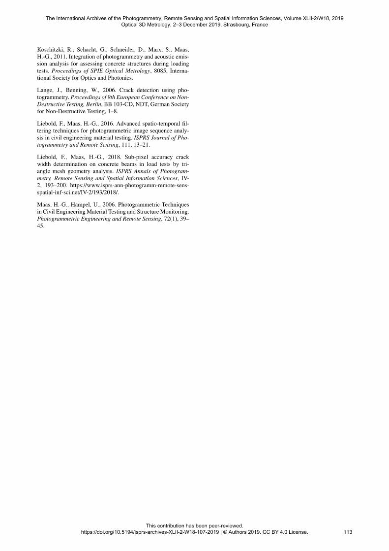
Fig. 15 shows the mean standard deviations σr of the crackwidths of each epoch where cracks are detected. Due to outliers,the mean standard deviation computed with the MAD σr,MAD

is also plotted. σr increases with higher crack widths becausethe outliers are small (close to δ) and greater values are moreinfluenced by these outliers. In contrast, σr,MAD is more orless stable over the time. σr,MAD is below 0.015 mm (corre-sponds to 0.15 px in image space) whereas σr reaches values upto 0.075 mm. Due to the outliers, σr,MAD should be preferredas a measure of precision.

Figure 15. Means of the standard deviations of the crack widthareas for each epoch.

5. CONCLUSION AND OUTLOOK

This publication presents a strategy for detection of cracks onconcrete specimens with non-planar surfaces in tension tests,and the computation of the according widths. A prerequisite isthat deformations only appear tangential to the surface. Theaccuracy of the crack widths depends on the quality of thedisplacement field and is in the same order of magnitude. Inour experiments, accuracies of approximately 0.01 mm werereached. The next step can be the development of an algorithmthat can determine crack opening vectors for cracks with signif-icant z-components. Further improvements should also allow toanalyze arbitrary 3D surfaces.

ACKNOWLEDGEMENTS

The research work presented in this publication has been per-formed within the research training group GRK-2250 at TUDresden funded by the German Research Council (DFG).

REFERENCES

Barazzetti, L., Scaioni, M., 2009. Crack measurement: De-velopment, testing and applications of an automatic image-based algorithm. ISPRS Journal of Photogrammetry and Re-mote Sensing, 64, 285–296.

Dare, P., Hanley, H., Fraser, C., Riedel, B., Niemeier,W., 2002. An Operational Application of Automatic Fea-ture Extraction: The Measurement of Cracks in ConcreteStructures. The Photogrammetric Record, 17(99), 453–464.http://dx.doi.org/10.1111/0031-868X.00198.

Gortz, S., 2004. Zum Schubrissverhalten von Stahlbeton- undSpannbetonbalken aus Normal- und Hochleistungsbeton. PhDthesis, RWTH Aachen.

Hampel, U., Maas, H.-G., 2009. Cascaded image analysis fordynamic crack detection in material testing. ISPRS Journal ofPhotogrammetry and Remote Sensing, 64(4), 345–350.

Heravi, A. A., Curosu, I., Mechtcherine, V., 2019. A gravity-driven split Hopkinson tension bar for investigating quasi-ductile and strain-hardening cement-based composites undertensile impact loading. Cement and Concrete Composites, n/a–n/a.

Irwin, G. R., 1958. Fracture. Springer Berlin Heidelberg,Berlin, Heidelberg, 551–590.



112

Koschitzki, R., Schacht, G., Schneider, D., Marx, S., Maas,H.-G., 2011. Integration of photogrammetry and acoustic emis-sion analysis for assessing concrete structures during loadingtests. Proceedings of SPIE Optical Metrology, 8085, Interna-tional Society for Optics and Photonics.

Lange, J., Benning, W., 2006. Crack detection using pho-togrammetry. Proceedings of 9th European Conference on Non-Destructive Testing, Berlin, BB 103-CD, NDT, German Societyfor Non-Destructive Testing, 1–8.

Liebold, F., Maas, H.-G., 2016. Advanced spatio-temporal fil-tering techniques for photogrammetric image sequence analy-sis in civil engineering material testing. ISPRS Journal of Pho-togrammetry and Remote Sensing, 111, 13–21.

Liebold, F., Maas, H.-G., 2018. Sub-pixel accuracy crackwidth determination on concrete beams in load tests by tri-angle mesh geometry analysis. ISPRS Annals of Photogram-metry, Remote Sensing and Spatial Information Sciences, IV-2, 193–200. https://www.isprs-ann-photogramm-remote-sens-spatial-inf-sci.net/IV-2/193/2018/.

Maas, H.-G., Hampel, U., 2006. Photogrammetric Techniquesin Civil Engineering Material Testing and Structure Monitoring.Photogrammetric Engineering and Remote Sensing, 72(1), 39–45.



113

crack width measurement for non-planar surfaces by ...€¦ · crack width measurement for...

Documents