IDENTIFICATION OF ELECTROMAGNETIC SCATTERING MECHANISMS BY TWO DIMENSIONAL WINDOWED FOURIER TRANSFORM

APPROACH

A THESIS SUBMITTED TO THE GRADUATE SCHOOL OF NATURAL AND APPLIED SCIENCES

OF MIDDLE EAST TECHNICAL UNIVERSITY

BY K. EGEMEN GERMEÇ

IN PARTIAL FULLFILLMENT OF THE REQUIREMENTS FOR

THE DEGREE OF MASTER OF SCIENCE IN

ELECTRICAL AND ELECTRONICS ENGINEERING

DECEMBER 2004

ii

Approval of the Graduate School of Natural and Applied Sciences

I certify that this thesis satisfies all the requirements as a thesis for the degree of Master of Science.

This is to certify that we have read this thesis and that in our opinion it is fully adequate, in scope and quality, as a thesis for the degree of Master of Science.

Examining Committee Members

ABSTRACT

Prof. Dr. smet Erkmen Head of Department

Prof. Dr. Mustafa Kuzuolu Supervisor

Prof. Dr. Canan Toker ( METU, EEE )

Prof. Dr. Kemal Leblebiciolu ( METU, EEE )

Prof. Dr. Mustafa Kuzuolu ( METU, EEE )

Assoc. Prof. Gülbin Dural ( METU, EEE )

Prof. Dr. Adnan Köksal ( HU, EE )

Prof. Dr. Canan Özgen Director

iii

I hereby declare that all information in this document has been obtained and presented in accordance with academic rules and ethical conduct. I also declare that, as required by these rules and conduct, I have fully cited and referenced all material and results that are not original to this work.

K. Egemen Germeç

iv

ABSTRACT

IDENTIFICATION OF ELECTROMAGNETIC SCATTERING MECHANISMS BY TWO DIMENSIONAL WINDOWED FOURIER TRANSFORM

APPROACH

GERMEÇ, Egemen

M.S. Department of Electrical and Electronics Engineering

Supervisor: Prof. Dr. Mustafa Kuzuolu

December 2004, 65 pages

In this thesis, it is demonstrated that the two-dimensional Windowed Fourier

Transform (WFT) can be effectively used to analyze the local spectral

characteristics of electromagnetic scattering signals in the two-dimensional spatial

frequency domain. The WFT is the extension of the Short Time Fourier

Transform (STFT), which was originally derived to analyze the local spectral

characteristics of one dimensional time functions. Since the WFT focuses on the

local spectral behavior of the scattered field, the signal localization maps

produced in the spectral domain by the WFT can be used to identify the

contributions of the rays, at a given location in space, arising from various

scattering mechanisms in high frequency applications.

Keywords: Windowed Fourier Transform, Electromagnetic Scattering

v

ÖZ

ELEKTROMANYETK SAÇINIM MEKANZMALARININ K BOYUTLU PENCERELENM FOURIER DÖNÜÜMÜ YÖNTEM LE

TANIMLANMASI

GERMEÇ, Egemen

Yüksek Lisans, Elektrik Elektronik Mühendislii Bölümü

Tez Yöneticisi: Prof. Dr. Mustafa Kuzuolu

Aralık 2004, 65 sayfa

Bu tezde, iki boyutlu Pencerelenmi Fourier Dönüümü (WFT) yönteminin, iki

boyutlu spektral frekans uzayında, elektromanyetik saçınım sinyallerinin lokal

spektral karakteristiklerini analiz etmek amacıyla etkili bir ekilde

kullanılabilecei gösterildi. Burada kullanılan WFT yöntemi, tek boyutlu ve

sadece zamana göre deien sinyallerin lokal spektral özelliklerini incelemek için

gelitirilmi olan Kısa Zamanlı Fourier Dönüüm (STFT) yönteminin gelitirilmi

biçimidir. WFT yöntemi saçınım alanlarının lokal spektral davranılarına

odaklandıı için, koordinatları verilen bir uzay noktasına karılık gelen spektral

uzaydaki sinyal yayılma haritaları WFT ile elde edilebilir. Bu haritalar yardımıyla

da, yüksek frekans uygulamalarında toplam elektromanyetik saçınım sinyalini

oluturan ve farklı mekanizmalardan kaynaklanan ıınların bireysel katkıları

belirlenebilir.

Anahtar Kelimeler: Pencerelenmi Fourier Dönüümü, Elektromanyetik Saçınım

vi

To My Family

vii

ACKNOWLEDGMENTS

The author wishes to express his deepest gratitude to his supervisor Prof. Dr.

Mustafa Kuzuolu for his guidance, advice, criticism, encouragements throughout

the research.

viii

TABLE OF CONTENTS

PLAGIARISM .................................................................................................III

ABSTRACT .....................................................................................................IV

ÖZ...................................................................................................................... V

ACKNOWLEDGMENTS ............................................................................. VII

TABLE OF CONTENTS..............................................................................VIII

LIST OF FIGURES.......................................................................................... X

CHAPTER

1. INTRODUCTION.......................................................................................... 1

1.1 Spatial Signal Analysis in Electromagnetic Scattering ............................... 1

1.2 The Windowed Fourier Transform (WFT)................................................. 2

1.3 Outline of This Thesis ............................................................................... 3

2. THEORY........................................................................................................ 4

2.1 Windowed Fourier Transform (WFT)........................................................ 4

2.1.1 Time-Frequency Signal Representations ............................................ 4

2.1.1.1 Time Analysis ........................................................................... 5

2.1.1.2 Frequency Analysis .................................................................... 5

2.1.1.3 Linear Time-Frequency Representations (TFRs) ........................ 6

ix

2.1.2 The Short-Time Fourier Transform (STFT)........................................ 6

2.1.2.1 Time-Dependent And Window-Dependent Uncertainty Principle 8

2.1.2.2 Analysis Window Selection ........................................................ 9

2.1.2.3 An Example for One Dimensional STFT .................................. 10

2.1.2.4 Space-Spatial Frequency Distributions...................................... 13

2.1.3 The Windowed Fourier Transform (WFT) ....................................... 13

2.1.3.1 Shannon Sampling Theorem and Nyquist Sampling Rate........ 13

2.1.3.2 Two Dimensional Windowed Fourier Transform...................... 15

2.1.3.3 An Example for the Two Dimensional WFT............................. 16

2.2 Electromagnetic Scattering ..................................................................... 20

2.2.1 Introduction ..................................................................................... 20

2.2.2 Mathematical Formulation ............................................................... 21

2.2.3 Dependence of the Scattering Characteristics to Object Geometry and

Material Properties.................................................................................... 26

2.2.4 Examples of Scattering Applications................................................ 28

2.2.4.1 The Circular Cylinder Scattering Problem ................................ 28

2.2.4.2 Rays of the Scattered Field ....................................................... 34

2.2.4.4 The Sommerfeld Half-plane Problem........................................ 40

x

3. UTILIZATION OF THE 2D WFT FOR THE IDENTIFICATION OF

SCATTERING MECHANISMS..................................................................... 43

4. CONCLUSIONS .......................................................................................... 62

REFERENCES ................................................................................................ 64

xi

LIST OF FIGURES

FIGURES

Figure 2.1 Time characteristic of the signal (Real part of the signal). ................. 11

Figure 2.2 Frequency characteristic of the signal (Magnitude of FFT of the

signal)................................................................................................................ 11

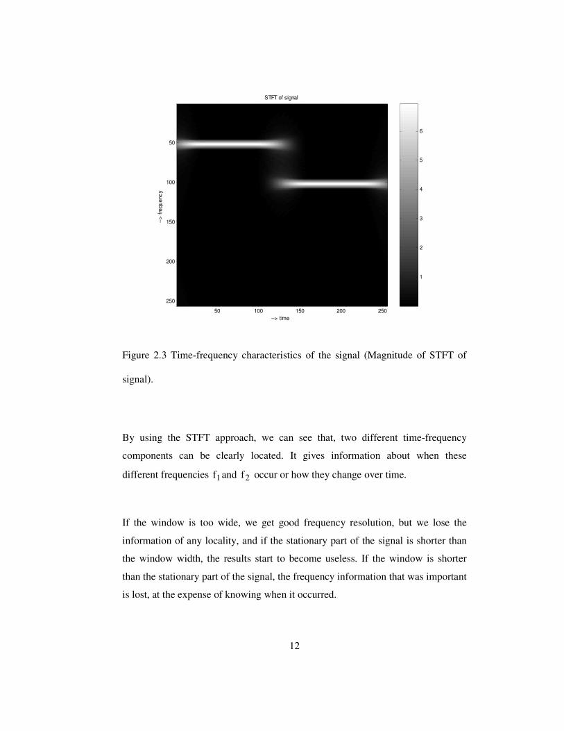
Figure 2.3 Time-frequency characteristics of the signal (Magnitude of STFT of

signal)................................................................................................................ 12

Figure 2.4 The csin function ( ) ( ) xxcxc /sinsin = ............................................. 15

Figure 2.5 Spatial characteristic of the 2D signal (Real part of the signal). ......... 17

Figure 2.6 Frequency characteristic of 2D signal (Magnitude of FFT of signal ). 17

Figure 2.7 Magnitude of 2D WFT of signal around center 5.1,5.1 == yx ......... 19

Figure 2.8 Magnitude of 2D WFT of signal around center 5.1,5.1 −=−= yx .... 19

Figure 2.9 Directions of E and H fields and the propagation............................ 22

Figure 2.10 A non-magnetic dielectric scatterer with permittivity ε and

permeability 0µ , occupying a region Ω in 3IR . .................................................. 23

Figure 2.11 An incident plane wave in the presence of a PEC circular cylinder. . 30

xii

Figure 2.12 The figure on the left shows the rays reflected by the circular cylinder,

and the rays of the shadow forming field. The figure on the right, shows the

diffracted rays emanating from ( )1,0 . ................................................................ 35

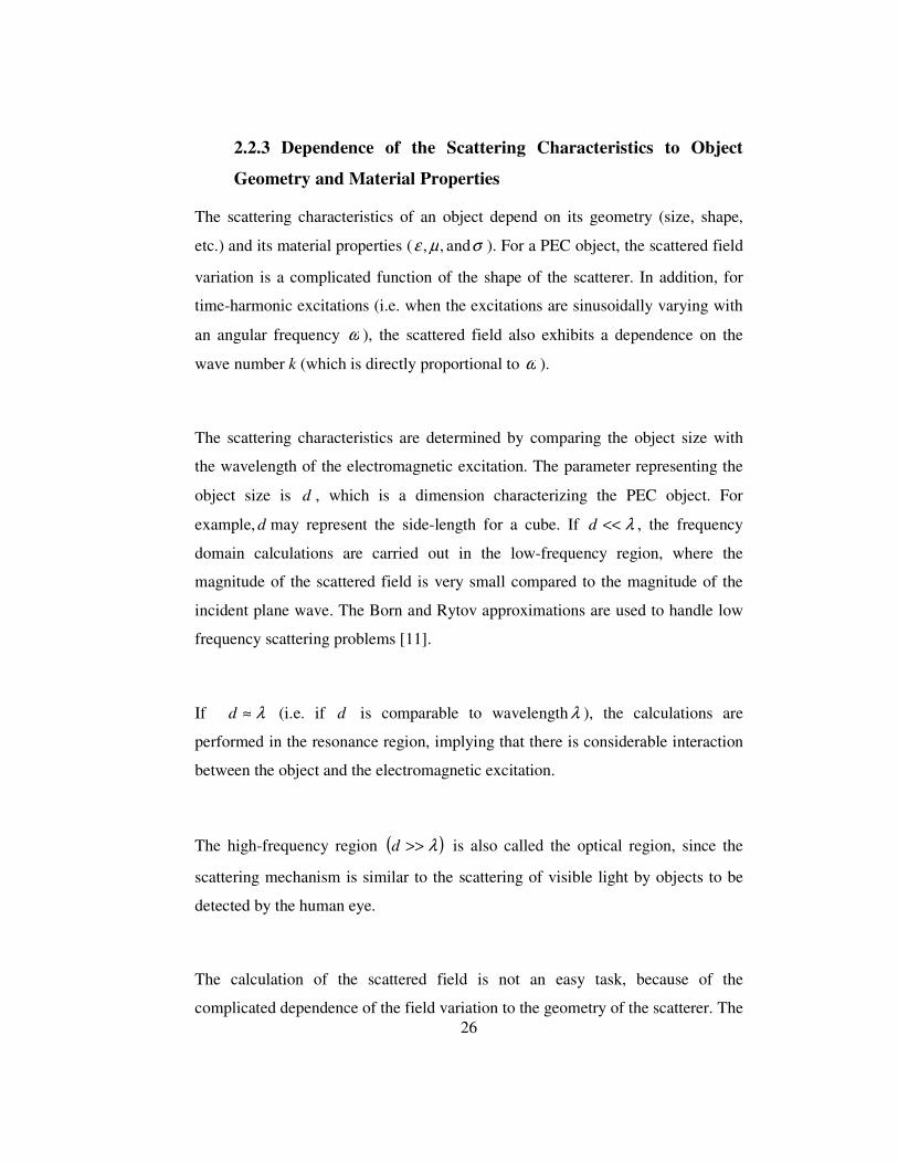
Figure 2.13 Geometrical explanation of the construction of reflected rays, where

Ra is the unit reflected ray vector and Ua is the unit normal vector. .................. 36

Figure 2.14 Geometrical explanation of the construction of diffracted rays,

emanating from ( )1,0 where Ta is the unit reflected ray vector and Na is the unit

normal vector..................................................................................................... 39

Figure 2.15 Geometrical explanation of the construction of diffracted rays,

emanating from ( )1,0 − where Ta is the unit reflected ray vector and Na is the unit

normal vector..................................................................................................... 40

Figure 2.16 The geometry of the Sommerfeld half-plane problem. ..................... 41

Figure 3.1 The real part of the scattered field ..................................................... 55

Figure 3.2 The absolute value of the Fourier transform of the scattered field...... 55

Figure 3.3 The real part of the total field ............................................................ 55

Figure 3.4 The absolute value of the Fourier transform of the scattered field...... 55

Figure 3.5 2D WFT of the scattered field with window center at x= 1.500,

y= 0.000 ............................................................................................................ 56

Figure 3.6 2D WFT of the scattered field with window center at x= 1.410,

y= 0.513 ............................................................................................................ 56

xiii

Figure 3.7 2D WFT of the scattered field with window center at x= 1.149,

y= 0.964 ............................................................................................................ 56

Figure 3.8 2D WFT of the scattered field with window center at x= 0.750,

y= 1.299 ............................................................................................................ 56

Figure 3.9 2D WFT of the scattered field with window center at x= 0.261,

y= 1.477 ............................................................................................................ 57

Figure 3.10 2D WFT of the scattered field with window center at x= -0.261,

y= 1.477 ............................................................................................................ 57

Figure 3.11 2D WFT of the scattered field with window center at x= -0.750,

y= 1.299 ............................................................................................................ 57

Figure 3.12 2D WFT of the scattered field with window center at x= -1.149,

y= 0.964 ............................................................................................................ 57

Figure3.13 2D WFT of the scattered field with window center at x= -1.409,

y= 0.513 ............................................................................................................ 58

Figure3.14 2D WFT of the scattered field with window center at x= -1.500,

y= 0.000 ............................................................................................................ 58

Figure3.15 2D WFT of the scattered field with window center at x= -1.410,

y= -0.513 ........................................................................................................... 58

Figure3.16 2D WFT of the scattered field with window center at x= -1.149,

y= -0.964 ........................................................................................................... 58

xiv

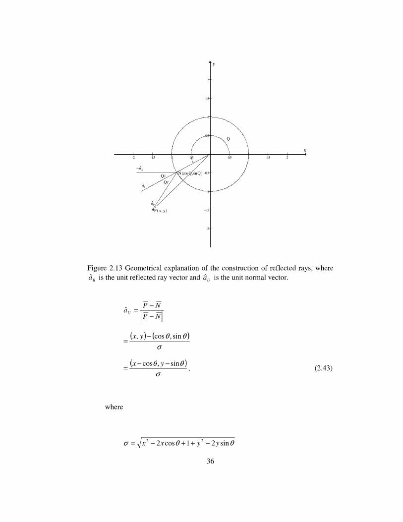
Figure 3.17 2D WFT of the scattered field with window center at x= -0.750,

y= -1.299 ........................................................................................................... 59

Figure 3.18 2D WFT of the scattered field with window center at x= -0.261,

y= -1.477 ........................................................................................................... 59

Figure 3.19 2D WFT of the scattered field with window center at x= 0.261,

y= -1.477 ........................................................................................................... 59

Figure 3.20 2D WFT of the scattered field with window center at x= 0.750,

y= -1.299 ........................................................................................................... 59

Figure 3.21 2D WFT of the scattered field with window center at x= 1.149,

y= -0.964 ........................................................................................................... 60

Figure 3.22 2D WFT of the scattered field with window center at x= 1.410,

y= -0.513 ........................................................................................................... 60

Figure 3.23 The real part of the scattered field ................................................... 61

Figure 3.24 The absolute value of the Fourier transform of the scattered field.... 61

Figure 3.25 The real part of the total field .......................................................... 61

Figure 3.26 The absolute value of the Fourier transform of the scattered field.... 61

1

CHAPTER 1

INTRODUCTION

1.1 Spatial Signal Analysis in Electromagnetic Scattering

In electromagnetic scattering applications, the scattered field is a vector-valued

function of the space coordinate variables. The field variation is a superposition of

several components related to the scattering mechanisms introduced by the

scattering object. These mechanisms become more pronounced when the scatterer

size is much larger than the wavelength. In this case, it is possible to interpret the

field variation in terms of ray optics. Therefore, at a certain point in space, it is

possible to express the field as a linear combination of rays emanating from the

scattering centers of the object [1].

The main aim of this thesis is to identify these rays from the values of the

scattered field. These values may be measured or numerically calculated by using

the well-known numerical solution techniques. In this thesis, it is demonstrated

that the Windowed Fourier Transform (WFT) can be utilized to extract the

information related to the ray-optical structure of the field variation.

The WFT provides the means to determine the local field behavior by yielding

the approximate plane wave directions. The theoretical basis of this result lies in

the representation of electromagnetic field components by plane wave expansions.

The validity of this approach is shown via two examples, namely the Sommerfeld

half-plane problem, and the scattering of a plane wave by an infinitely long

circular perfectly conducting cylinder. In these examples, it has been possible to

identify the ray directions by the WFT approach.

2

1.2 The Windowed Fourier Transform (WFT)

It is well-known that the Fourier transform (FT) )(ωX of a function

)(tx yields the spectral characteristics of that function via the expression

∞

∞−−= dttjtxX )exp()()( ωω (1.1)

In several applications, the independent variable t is interpreted as time, and

correspondingly ω represents the angular frequency. The Fourier transform of a

function is the inner product of )(tx with the complex exponential function

)exp( tjω , which, when interpreted as a projection in the function space,

represents the weight of the function )exp( tjω in the spectral representation of

)(tx . It is important to note that )(tx is used globally in the expression of the

Fourier transform and in order to extract the local spectral information, the Short

Time Fourier Transform (STFT) has been introduced [2]. The STFT of a function

)(tx is obtained by evaluating the FT of )(tx multiplied by a window function

)(tw which slides along the time axis, as shown in (1.2) below:

∞

∞−′′−′−′= tdtjtxttwtX )exp()()(),( ωω (1.2)

The window function )(tw is a function which is non-zero over a finite duration

and the time localization of the function )(tx is achieved by the product

)()( txttw ′−′ . It is clear that the STFT of )(tx is the Fourier transform of

)()( txttw ′−′ .

3

The STFT is a well-known example of a class of signal processing approaches

known as time-frequency representations. However, there are several applications

where the independent variable is not time. For instance, the independent variable

may be one of the space coordinates for representing spatial variations of a

quantity. In this case, the term STFT is replaced by the Windowed Fourier

Transform (WFT), which yields the local spectral characteristics of a function

whose independent variable is not time in general. If the independent variable is a

space coordinate, the WFT is a representation yielding the space vs. spatial

frequency variation of that function.

The higher dimensional versions of the WFT may be used in the analysis of

functions representing spatial variations in two- or three-dimensional space. In

this thesis, the WFT is used to analyze the electromagnetic field variations in

scattering applications, for the identification of the local ray directions. This

information is closely related to the geometric properties of the scatterer, and ray

directions may be used to identify the scattering centers (i.e. those points from

which the rays emanate) [3-5].

1.3 Outline of This Thesis

The first chapter of this thesis contains the introductory information related to the

thesis work. The theoretical analysis related to scattered field calculations and the

WFT is given in the second chapter. The examples validating the theoretical work

are demonstrated in the third chapter. Finally, the fourth chapter is devoted to the

conclusions.

4

CHAPTER 2

THEORY

2.1 Windowed Fourier Transform (WFT)

2.1.1 Time-Frequency Signal Representations

In real-time signal analysis, the Fourier transform is one of most widely used

signal-analysis tool [6]. The basic idea behind the Fourier transform is that any

arbitrary signal can be expressed as a superposition of weighted sinusoidal

functions. Since its value at a particular frequency is a measure of the similarity of

the signal to the sinusoidal basis at that frequency, the frequency attributes of the

signal are exactly described.

While the Fourier transform is a very useful concept, the Fourier transform does

not explicitly indicate how the frequency content of a signal evolves in time,

since the sinusoidal basis functions spread into the entire time domain and are

not concentrated in time.

Many signals, mostly the non-stationary signals, encountered in real world

situations have frequency content that changes over time. Because of the need to

represent this particular nature of the signal, joint time-frequency transforms have

been developed that reflects the behavior of the time-varying frequency content of

the signal [7].

The spectrum, obtained from the Fourier transform technique, allows us to

determine the frequency components that exist for the whole duration of the

signal but a joint time-frequency analysis allows us to determine the

5

frequency components at a particular time, so that the frequencies of the

dominant sinusoidal components can be displayed at each time instant.

A natural way of characterizing a signal simultaneously in time and frequency

domains, based on the expansion and inner product concepts, is to compare

elementary functions that are concentrated in both time and frequency

domains with the signal.

2.1.1.1 Time Analysis

Time analysis is the investigation of the properties of time-varying

quantities. Fundamental physical quantities, such as electric and magnetic

fields, change as a function of time and one can call these functions of time

as signals, or time waveforms, denoted by the symbol )(tx .

Time analysis techniques provide the information related to the time variation of

that particular quantity, such as its magnitude at specific time instants, its rate of

change with respect to time, its duration, …etc. In order to obtain further

information about the signal, it is essential to study the signal in terms of a

different representation. A powerful approach in this direction is the spectral

representation, which is called frequency analysis.

2.1.1.2 Frequency Analysis

In order to extract further information about a signal, frequency analysis

or spectral analysis, is a major requirement. Frequency analysis provides

the information related to the frequency content of a signal via the

Fourier transform.

6

2.1.1.3 Linear Time-Frequency Representations (TFRs)

In many signal processing applications, separate time and frequency analysis

approaches may not be sufficient. In these cases, it may be useful to combine

these two methods to yield the Time-Frequency Representations (TFRs). For

any function )(tx , a corresponding TFR ),( ftTx may be obtained, which

basically is a representation of the spectral behavior of that signal localized at

t .

An important subset of TFRs is a group of representations known as linear

TFRs. Linear TFRs satisfy the superposition or linearity principle which states

that if )(tx is a linear combination of some signal components, then the TFR of

)(tx is the same linear combination of the TFRs of individual signal

components by the same weights.

),(),(),()()()(21 212211 ftTcftTcftTtxctxctx xxx +=+= (2.1)

Linearity is a desirable property in many applications involving multi-

component signals, especially when the isolation of the signal components is

needed. The Short-time Fourier Transform is the mostly used linear TFR used to

study non-stationary signals [8].

2.1.2 The Short-Time Fourier Transform (STFT)

The Fourier Transform does not give any information on the time interval over

which a particular frequency component exists. It does not explicitly reflect the

time-varying nature of a signal. It only indicates the presence of various

frequency components within the signal, since the basis functions used in the

7

classical Fourier analysis cannot be associated with any particular time

instant.

The motivation behind the Short-Time Fourier Transform (STFT) is to obtain the

frequency content at a particular time. To this end, the signal is localized around that

time instant and Fourier analysis is carried out over this localized signal, neglecting

the rest of the signal. Since the time interval which is the support of the

localized signal is short compared to the whole signal, this process is called Short-

Time Fourier Transform.

The STFT is a formulation that can represent signals of arbitrary duration by

breaking them into sub-signals of shorter durations, and applying the FT to each

sub-signal. It is based upon a series of overlapped and segmented Fourier

transforms that occur across the data stream. In the STFT, the individual Fourier

transforms from these multiple segments give a good indication of the time-

frequency properties of the signal.

The STFT of a signal )(tx is defined as [9],

tdtfjttwtxftX wSTFT ′′−−′′=

∞

∞−)2exp()()(),()( π (2.2)

where )(tx is a time signal and )(tw is a suitably chosen window function.

The function )(tw could be simply a rectangular pulse of finite duration, although

often a Gaussian or Hamming function is used in order to get rid of the undesired

effects of the Gibbs phenomenon [10]. The window function simply limits the

8

duration over which the Fourier Transform occurs. This window is then translated

along the time axis. By moving )(tw and repeating the same process, one could

obtain an idea about the evolution of the frequency contents of the signal.

2.1.2.1 Time-Dependent And Window-Dependent Uncertainty

Principle [ 6 ]

The time-bandwidth product theorem, or Heisenberg uncertainty principle, has

played a prominent role in discussions of joint time-frequency analysis.

According to this principle, the product of time and frequency resolution is always

greater than a minimum value. The uncertainty principle for the short-time Fourier

transform is a function of time, the signal, and the window. Since the uncertainty

principle prohibits the existence of windows with arbitrarily small duration and

arbitrarily small bandwidth, the joint time-frequency resolution of the short time

Fourier transform is inherently limited.

From the original signal )(tx , one defines a short duration signal around the time of

interest t by multiplying it by a window function that is peaked around the

time t and falls off rapidly. This has the effect of emphasizing the signal at time t

and suppressing it for times far away from that time.

The choice of a window function indicates both the time and the frequency

resolution for the entire representation. Since there is an inherent trade-off

between time and frequency localization in short time Fourier transform for a

particular window, the window function cannot be chosen arbitrarily. The degree

of trade-off depends on the window, signal, time, and frequency.

To summarize, in STFT applications, narrow window means good time resolution

but poor frequency resolution and wide window means poor time resolution but

9

good frequency resolution. For a given window, time and frequency resolution of

STFT is fixed.

2.1.2.2 Analysis Window Selection

Since the choice of the analysis window directly affects the trade-off between

frequency resolution and time resolution as well as the side-lobe attenuation, one

has to know the effect of the window.

Let us examine such effects based on a complex exponential signal given in

discrete time domain as

njwAenx 0)( = (2.3)

If one multiplies this signal with a window function )(nw and takes the discrete

time Fourier transform of the resulting product, one obtains the result stated

below:

( ) −=n

jwnW enwnxwX ).()( (2.4)

−−=n

nwwjenwA )( 0).( (2.5)

)( 0wwAW −= (2.6)

where )(wW is the discrete-time Fourier transform of the window.

10

So, the transform of a windowed sinusoid is equal to the transform of the window

function shifted by an amount equal to the frequency of the sinusoid.

2.1.2.3 An Example for One Dimensional STFT

In the following example, we use a Hamming window but other windows can also

be used. Once we have decided on a window function and a window length, we

can compute the DFT of this frame. The number of samples of DFT should at

least be equal to the window length, with any additional samples being produced

via zero padding. The details of the STFT approach are demonstrated in the

example given below, based on a joint time-frequency signal representation.

Consider a time domain signal )(tx , which is plotted in Figure 2.1, consisting of

sinusoids with two different frequencies, the first one with a frequency Hz50f1 =

existing over an interval [ ]128,1T1 = seconds, and the second one with a frequency

Hz100f2 = existing over the interval [ ]256,129T2 = seconds. The Fourier

transform of )(tx is computed and presented in Figure 2.2. It is clearly seen that

the plot for the magnitude of the FT indicates the presence of two distinct

frequency components of frequencies 1f and 2f . But it does not give any

information about the time range over which a specific frequency component

exists.

=)..2exp(

)..2exp()(

2

1

xfj

xfjtx

ππ

256129

1281

≤≤≤≤

t

t (2.7)

One approach, which can give information on the time localization of the

spectrum, is the short-time Fourier transform.

11

In this example, STFT is computed using a MATLAB code, and the magnitude of

the STFT output is plotted in Figure 2.3.

0 50 100 150 200 250-1

-0.8

-0.6

-0.4

-0.2

0

0.2

0.4

0.6

0.8

1real(signal)

--> time

Figure 2.1 Time characteristic of the signal (Real part of the signal).

0 50 100 150 200 2500

50

100

150abs(fft(signal))

--> frequency

Figure 2.2 Frequency characteristic of the signal (Magnitude of FFT of the

signal).

12

STFT of signal

--> time

--> fr

eque

ncy

50 100 150 200 250

50

100

150

200

250

1

2

3

4

5

6

Figure 2.3 Time-frequency characteristics of the signal (Magnitude of STFT of

signal).

By using the STFT approach, we can see that, two different time-frequency

components can be clearly located. It gives information about when these

different frequencies 1f and 2f occur or how they change over time.

If the window is too wide, we get good frequency resolution, but we lose the

information of any locality, and if the stationary part of the signal is shorter than

the window width, the results start to become useless. If the window is shorter

than the stationary part of the signal, the frequency information that was important

is lost, at the expense of knowing when it occurred.

13

2.1.2.4 Space-Spatial Frequency Distributions

In some applications, the signal to be analyzed may be a function of one or

more space variables. Then, in contrast to the conventional frequency

concept used in the spectral analysis of time signals, the variables in the

Fourier transform will be spatial frequencies. In this case, the STFT

approach is replaced by the WFT as explained below.

2.1.3 The Windowed Fourier Transform (WFT)

To extract local-frequency information from a signal (the independent variable

may be time, space coordinate, …etc.) , the Windowed Fourier Transform represents

an analysis technique. The approach is identical to the STFT in the sense that a

sliding window function is used in the FT to obtain the local spectral properties.

2.1.3.1 Shannon Sampling Theorem and Nyquist Sampling Rate

According to the Shannon sampling theorem, it is possible to reconstruct a

function exactly from its samples, provided that the function is band-limited and

the sampling frequency is sufficiently high to resolve its highest frequency

components.

The sampling theorem gives a directive for selecting sufficiently small grid

spacing x∆ once the band-limit Ω is known. It states that x∆ must be chosen

to satisfy the critical sampling rate Ω

=∆ 1X which is called the Nyquist

sampling rate and the frequency 2Ω

is known as the Nyquist frequency. The

Nyquist frequency is the highest frequency that can be resolved using a given

sample spacing x∆ and all higher frequencies will be aliased to lower

frequencies. The Nyquist sampling rate is the largest grid spacing that can

14

resolve the frequency and this also implies that in order to resolve a single

sinusoidal function, one must have at least two sample points per period of the

wave.

Assume that f is a band-limited function whose Fourier transform is zero

outside of the interval

−2

,2

nn. If x∆ is chosen as:

Ω<∆ 1

X , (2.8)

then f may be reconstructed exactly from its samples as follows

)()( nn xfxnff =∆= (2.9)

∆−=

∞

−∞= xxx

cfxf n

nn

)(sin)(

π =

∞

−∞= −∆−∆

n n

nn xx

xxxfx

)()/)(sin(

ππ

(2.10)

where the sinc function is given by ( )x

xxc

)sin(sin = , shown in Figure 2.4

below.

15

-8 -6 -4 -2 0 2 4 6 8-0.4

-0.2

0

0.2

0.4

0.6

0.8

1

--> x

-->

sinc

(x)

Figure 2.4 The csin function ( ) ( ) xxcxc /sinsin =

2.1.3.2 Two Dimensional Windowed Fourier Transform

The two dimensional windowed Fourier transform of a signal ( )yxf , is defined

by

( ) ( ) ( ) ( ) βαβαβα βα ddeyxwfkkyxWFT yx kjkyxf

+−−−= ,,,,, (2.11)

where ( )βα ,w denotes a two-dimensional, usually even and real-valued, window

function.

The standard procedures used to realize one dimensional WFT approaches, can be

suitably generalized to the two dimensional case as demonstrated in the example

below.

16

2.1.3.3 An Example for the Two Dimensional WFT

Consider a spatial signal, as shown in Figure 2.5, consisting of two localized

sinusoids with frequencies ( )11, fyfx and ( )22 , fyfx .

The first component has frequency ( )mfx /1101 = and ( )mfy /101 = existing over

an interval [ ]2,0=x meters and [ ]2,0=y meters (Region 1) and the second a

frequency ( )mfx /1202 = and ( )mfy /102 = existing over another interval

[ ]0,2−=x meters and [ ]0,2−=y (Region 3).

The Fourier Transform gives two approximate 2D sinc functions without any

implication of localization. Space and frequency characteristics of the signal are

different in the regions below:

0&0:1Region >> yx

0&0 x:Region2 >< y

0&0 x:Region3 << y

0y&0x:Region4 <>

We simulate this 2D signal, which exists in [ ]2,2 +−=x and [ ]2,2 +−=y with

256x256 samples by a Matlab code.

17

- 2 - 1 . 5 - 1 - 0 . 5 0 0 . 5 1 1 . 5 2- 2

- 1 . 5

- 1

- 0 . 5

0

0 . 5

1

1 . 5

2

x ( m )

y (m

)

Figure 2.5 Spatial characteristic of the 2D signal (Real part of the signal).

- 3 0 - 2 0 - 1 0 0 1 0 2 0 3 0- 3 0

- 2 0

- 1 0

0

1 0

2 0

3 0

f x ( 1 / m )

fy (1

/m)

2 0 0 0

4 0 0 0

6 0 0 0

8 0 0 0

1 0 0 0 0

1 2 0 0 0

1 4 0 0 0

1 6 0 0 0

Figure 2.6 Frequency characteristic of 2D signal (Magnitude of FFT of signal ).

18

In this example, we use a Hamming window in the Matlab code, but other

windows can possibly be used. Once we have decided on a window function and a

length, we can compute the 2D DFT of this frame. The size of this 2D DFT is

chosen to be at least window length, with any additional samples being produced

via zero padding.

One approach, which can give information on the space resolution of the

spectrum, is the 2D WFT. A moving 2D window can be applied to the signal and

the Fourier transform is applied to the signal within the window as the window is

moved.

In order to have an idea of what can be achieved by the 2D WFT, the following

results are obtained. The grid is x256256 and the window function is Hamming

with a length occupying 65 samples in x and y .

The 2D WFT is evaluated at [ ]5.1,5.1 == yx , which is in the first region, and

then at [ ]5.1,5.1 −=−= yx which is in the third region.

When we plot the windowed Fourier Transform at [ ]5.1,5.1 == yx which is in the

first region, we can see only the frequency characteristic of the signal focused

around ( )11, fyfx , as shown in Figure 2.7, and when we plot the windowed

Fourier Transform around center [ ]5.1,5.1 −=−= yx , which is in the second

region, we can see only the frequency characteristic of the signal focused around

( )22 , fyfx as expected, as shown in Figure 2.8.

19

- 3 0 - 2 0 - 1 0 0 1 0 2 0 3 0- 3 0

- 2 0

- 1 0

0

1 0

2 0

3 0

f x ( 1 / m )

fy (1

/m)

1 0 0

2 0 0

3 0 0

4 0 0

5 0 0

6 0 0

7 0 0

8 0 0

9 0 0

1 0 0 0

1 1 0 0

Figure 2.7 Magnitude of 2D WFT of signal around center 5.1,5.1 == yx

- 3 0 - 2 0 - 1 0 0 1 0 2 0 3 0- 3 0

- 2 0

- 1 0

0

1 0

2 0

3 0

f x ( 1 / m )

fy (1

/m)

1 0 0

2 0 0

3 0 0

4 0 0

5 0 0

6 0 0

7 0 0

8 0 0

9 0 0

1 0 0 0

1 1 0 0

Figure 2.8 Magnitude of 2D WFT of signal around center 5.1,5.1 −=−= yx

20

As a result, by using the 2D WFT, we can see that the two space-frequency

components can be clearly identified, located around the locus of the two

frequencies. It gives information about when these different frequencies ( )11, fyfx

and ( )22 , fyfx , occur or how they change over the spatial domain.

2.2 Electromagnetic Scattering

2.2.1 Introduction

If an electromagnetic wave is incident on an object, which may be perfectly

conducting or dielectric, the wave is scattered because of the presence of the

object. The sum of the incident and the scattered fields form the total field.

Most of the scattering problems can not be solved exactly due to the complex

shape (or material parameter variations) of the scatterer, and approximate

numerical approaches are used to analyze scattering problems. The most well-

known approaches are

1. Finite Difference Time Domain (FDTD) method [12],

2. Method of Moments (MoM) [13],

3. Finite Element Method (FEM) [14].

Finite Difference Time Domain (FDTD) method is one of the most successful

numerical approaches to the direct solution of Maxwell’s curl equations governing

the electric and magnetic field in time domain.

21

Method of Moments (MoM) is used to solve a certain class of integro-differential

equations to analyze (mostly) perfectly conducting structures.

Finite Element Method (FEM) is commonly used for modeling complex, in-

homogenous structures for the solution of the Maxwell’s differential equations. In

this method the unknown function is approximated on a domain, which is

represented by a set of elements of simple shape with a finite number of

parameters.

2.2.2 Mathematical Formulation

In scattering problems the incident field is usually taken as a plane wave given by

).ˆexp(ˆ)( rijkerE ii −= (2.12)

The amplitude iE is chosen to be 1 (volt/m), λπεµ /)2(00 == wk is the wave

number, λ is a wavelength in the medium, i is a unit vector in the direction of

wave propagation, and ie is a unit vector in the direction of its polarization [11].

Associated with iE , there is a magnetic field iH , which is perpendicular to iE ,

given by:

).ˆexp()ˆxˆ()( rijkeirH ii −= (2.13)

22

Figure 2.9 Directions of E and H fields and the propagation.

Both iE and iH satisfy Maxwell’s curl equations in free space:

ii HjwE 0x µ−=∇ (2.14.a)

ii EjwH 0x µ−=∇ (2.14.b)

If iH is eliminated, iE satisfies the homogeneous vector wave equation given

by:

0)xx( 2 =−∇∇ ii EkE (2.15)

Now, consider a non-magnetic dielectric object with permittivity ε and

permeability 0µ , occupying a region Ω in 3R , as shown in Figure 2.10 below.

iei ˆxˆ

ie

i

23

iE , iH

sE , sH Ω

Figure 2.10 A non-magnetic dielectric scatterer with permittivity ε and permeability 0µ , occupying a region Ω in 3IR .

where the incident field components are given by the equations ( )13.212.2 − in

the absence of the scattering object and ( )ss HE , are the scattered field

components whose sources are in Ω .

The total field components ( )tt HE , are defined as:

sit EEE += (2.16.a)

sit HHH += (2.16.b)

which satisfy:

tt HjwE µ−=∇x (2.17.a)

24

tt EjwH ε−=∇x (2.17.b)

where 0µµ = everywhere and 0εε = outside Ω and εε ˆ= within Ω .

After substituting ( )16.2 in ( )17.2 , the following equations are obtained

)()x( 0 sisi HHjwEE +−=+∇ µ everywhere (2.18.a)

)()(x 0 sisi EEjwHH +=+∇ ε outside Ω (2.18.b)

)(ˆ)(x sisi EEjwHH +=+∇ ε inside Ω (2.18.c)

Using ( )16.2 and ( )ba 18.218.2 − , the following equation is generated:

ss HjwE 0x µ−=∇ (2.19.a)

ss EjwH 0x ε−=∇ outside Ω (2.19.b)

Finally, for the scattered field inside Ω , we obtain

25

sisi EjwEjwHH εε ˆˆxx +=∇+∇ (2.19c)

and using ( )13.2 , we obtain:

sis EjwEjwH εεε ˆ)ˆ(x 0 +−=∇ inside Ω (2.19d)

The term iEjw )ˆ( 0εε − acts as a source term for the scattered field [15].

Equations ( )cba 19.219.219.2 −− are the governing partial differential equations

of the scattered field. It is noted that outside the scatterer, the equations turn out to

be free-space Maxwell’s equations, and inside the scatterer, the equation ( )d19.2

is not homogenous, containing a source term creating the scattered field.

If Ω represents a PEC object, the total field vanishes within Ω and the scattered

field satisfies ( )a19.2 and ( )b19.2 . The sources of the scattered field lie on Ω∂

(representing the boundary of Ω ) and they are represented by the boundary

condition

)xˆ()xˆ( is EnEn −= (2.19e)

where n is the unit outward normal on Ω∂ .

26

2.2.3 Dependence of the Scattering Characteristics to Object

Geometry and Material Properties

The scattering characteristics of an object depend on its geometry (size, shape,

etc.) and its material properties ( ,, µε andσ ). For a PEC object, the scattered field

variation is a complicated function of the shape of the scatterer. In addition, for

time-harmonic excitations (i.e. when the excitations are sinusoidally varying with

an angular frequency ω ), the scattered field also exhibits a dependence on the

wave number k (which is directly proportional to ω ).

The scattering characteristics are determined by comparing the object size with

the wavelength of the electromagnetic excitation. The parameter representing the

object size is d , which is a dimension characterizing the PEC object. For

example, d may represent the side-length for a cube. If λ<<d , the frequency

domain calculations are carried out in the low-frequency region, where the

magnitude of the scattered field is very small compared to the magnitude of the

incident plane wave. The Born and Rytov approximations are used to handle low

frequency scattering problems [11].

If λ≈d (i.e. if d is comparable to wavelength λ ), the calculations are

performed in the resonance region, implying that there is considerable interaction

between the object and the electromagnetic excitation.

The high-frequency region ( )λ>>d is also called the optical region, since the

scattering mechanism is similar to the scattering of visible light by objects to be

detected by the human eye.

The calculation of the scattered field is not an easy task, because of the

complicated dependence of the field variation to the geometry of the scatterer. The

27

analytical solution of scattering problems can be obtained only for a few specific

cases. The field scattered by a PEC sphere or an infinite cylinder for plane wave

incidence, can be obtained by solving the governing partial differential equations

by using separation of variables and the complete solution is obtained in the form

of an infinite series [15].

There are other problems such as the Sommerfield half-plane problem, or the edge

scattering problem, that can be solved analytically. If the analytical solution is not

achievable, one may try to obtain an approximate solution via FEM, MoM or

FDTD as explained earlier. In all these methods, the computational domain is

discretized (i.e. it is represented as a union of smaller sub-domains) and the

unknown function (which is either E and H field variation, or an equivalent

surface or volume current density, J ). Finally, the integral or differential equation

is solved approximately, yielding the unknowns. The numerical solution

techniques are effective for low or medium frequency range, and for high

frequency applications they become formidable, because of the necessity to

employ a large number of unknowns to model the problem. For high frequency

applications, methods based on ray-optical approaches are quite popular, and the

most well-known ray-optical approach is the Geometric Theory of Diffraction

(GTD) introduced by Keller [3].

The geometrical theory of diffraction is an extension of geometrical optics,

which accounts for diffraction. It introduces diffracted rays in addition to

the usual rays of geometrical optics. These rays are produced by incident rays

which hit edges, corners, or vertices of boundary surfaces or which graze such

surfaces.

Various laws of diffraction, analogous to the laws of reflection and refraction,

are employed to characterize the diffracted rays. A modified form of Fermat's

28

principle, equivalent to these laws, can also be used. Diffracted wave fronts

are defined, which can be found by a Huygens wavelet construction. There is

an associated phase or eikonal function, which satisfies the eikonal equation. In

addition, complex or imaginary rays are introduced. A field is associated with

each ray and the total field at a point is the sum of the fields on all rays

through the point. The phase of the field on a ray is proportional to the optical

length of the ray from some reference point. The amplitude varies in

accordance with the principle of conservation of energy in a narrow tube of

rays. The initial value of the field on a diffracted ray is determined from the

incident field with the aid of an appropriate diffraction coefficient. These

diffraction coefficients are determined from certain canonical problems. They

all vanish, as the wavelength tends to zero.

2.2.4 Examples of Scattering Applications

In this section, two scattering problems will be studied, namely i) the scattering of

a zTM plane wave by an infinite PEC circular cylinder whose axis is paralled to

the z -axis, and ii) the Sommerfeld half-plane problem. In both cases, the ray

optical approach will be underlined, since our ultimate aim is to identify the ray

directions by the 2D WFT.

2.2.4.1 The Circular Cylinder Scattering Problem

Consider the diffraction of a plane electromagnetic wave by an infinite conducting

cylinder of radius a as shown in Figure 2.11. Let ),,( zr ϕ be a system of

cylindrical coordinates such that the z -axis coincides with the axis of the cylinder

and the angle ϕ is measured from the direction of propagation of the incident

wave. We assume that the time dependence is described by the factor )exp( tjω ,

where ω is the angular frequency of the incident field, and that the electric field

vector of the incident wave is parallel to the axis of the cylinder.

29

Then the problem reduces to finding the complex amplitude of the scattered field

E satisfying Helmholtz’s equation

011 2

2

2

2 =+∂∂+

∂∂

∂∂

EkE

rrE

rr ϕ

(2.20)

and the boundary condition

0)cosexp(0 =−+= ϕjkaEE ar (2.21)

The solution of our problem has the form

∞

=

=0

)2( cos)(n

nn nkrHNE ϕ (2.22)

where the Hankel function is defined as )()()()2( krjYkrJkrH nnn −= .

The unknown coefficients can be evaluated by using the boundary condition and

the following equality, which gives the incident field:

∞

=−+=−

10 cos)()(2)()cosexp(

nn

n nkaJjkaJjka ϕϕ (2.23)

30

Therefore, the required solution for the scattered field is given by:

−+−=

∞

=1

)2()2(

)2(0)2(

0

00 cos)(

)()(

)(2)()(

)(

nn

n

nn nkrHkaH

kaJjkrH

kaHkaJ

EE ϕ

(2.24)

x

y

Incident wavea

Figure 2.11 An incident plane wave in the presence of a PEC circular cylinder.

The series solution is exact in the sense that the series expansion yields the

analytical solution for all frequencies. The ray-optical approach may be applied

for the case where λ>>a2 as outlined below.

Let us denote the scattered field by su and the total field by u . The asymptotic

theory is based on geometrical optics and the geometrical theory of diffraction [4-

5]. In the asymptotic theory, one seeks the solution for su in sjkx ueu += − , as a

superposition of the form:

31

=

=L

l

yxjkSl

s leyxAyxu1

),(),(),( (2.25)

Here L denotes the number of fields. In our specific example, the sum consists of

a reflected field and possibly one or two diffracted fields, and a shadow forming

field.

Each field ),(),( yxjkSeyxA is a solution to the equation

02 =+∇ uku (2.26)

where, A is called the amplitude, k is the wavenumber, ),( yxjkSe is the phase

factor, and S is the phase. To determine the phase of each field we can use the

methods of the asymptotic theory. First we substitute ),(),( yxjkSeyxA into

02 =+∇ uku and cancel the phase factor to obtain:

0.2]1)[( 22 =∇+∇+∇∇+−∇− ASikAASikASk (2.27)

Equating the leading order term of equation ( )27.2 , to zero, yields the eikonal

equation of geometrical optics:

01)( 2 =−∇S . (2.28)

32

This is a first order non-linear partial differential equation for the phase S , which

we can solve by the method of characteristics. To do so, we introduce the two-

parameter family of characteristic curves or rays ),( τσX , ),( τσY and the

equations

xSd

dX =σ

τσ ),(, yS

ddY =

στσ ),(

. (2.29)

In this case,

)(τxx SS ≡ and )(τyy SS ≡ (2.30)

are independent of the arc-length σ , because the index of refraction is a constant.

Hence the rays propagate along straight lines in the direction S∇

)(),0(),( τσττσ xSXX += , (2.31a)

)(),0(),( τσττσ ySYY += (2.31b)

On each ray, the phase is determined from the equation

1),( =

στσ

ddS

(2.32)

σττσ += )(),( 0SS (2.33)

33

The initial condition Γ= |)(0 SS τ is determined on the surface of the

scatterer )(τΓ :

)),0(),,0(()( τττ YX=Γ (2.34)

From the boundary condition

jkxs eu −−= , Γ∈),( yx (2.35)

for the reflected field,

),0()(0 ττ XS = (2.36)

Arguments pertaining to the geometrical theory of diffraction yield )(0 τS for the

diffracted fields.

To determine the ray direction )(0 τS∇ we use

01)( 2 =−∇S (2.37)

34

and the strip condition on Γ

ττ

ττ

ττ

ddY

SddX

Sd

dSyx )()(

)(0 += (2.38)

2.2.4.2 Rays of the Scattered Field

The scattered field consists of four terms

−+ +++= ddsfRS uuuuu , (2.39)

which are the reflected field Ru , the shadow forming field sfu , the diffracted field

+du originating at ( )1,0 , and the diffracted field −du originating at ( )1,0 − . The

fields Ru and sfu satisfy the boundary conditions

( ) jkxR eyxu −−=, ( ) Γ∈yx, 0<x , (2.40)

( ) jkxsf eyxu −−=, ( ) Γ∈yx, 0≥x . (2.41)

Both diffracted fields vanish on the surface of the cylinder. The field sfu in the

region 0≥x , 1≤y is called the shadow forming field because sfu + iu vanishes

in that region.

35

The rays

( ) τσττσ 2coscos, −=X 2/32/ πτπ ≤≤ (2.42a)

( ) τσττσ 2sinsin, −=Y 2/32/ πτπ ≤≤ (2.42b)

are shown in the Figure 2.12 below.

Figure 2.12 The figure on the left shows the rays reflected by the circular cylinder, and the rays of the shadow forming field. The figure on the right, shows the diffracted rays emanating from ( )1,0 .

For reflected rays, if we find out the angle, θτ = , for each point, ( )yx, , in the

suggested regions , we can determine corresponding reflected rays by using the

equations given below:

36

x(t)=cos t , y(t)=sin t

x(t)=cos t/2 , y(t)=sin t/2

f(x)=1.5773x-cos((209.134/180)pi)

f(x)=-0.48

f(x)=0.5574x

f(x)=x

-2 -1.5 -1 -0.5 0.5 1 1.5 2

-2

-1.5

-1

-0.5

0.5

1

1.5

2

x

y

P ( x , y )

N (cos Q ,sin Q )

Q

Q iQ r

Ua

Ra

Xa−

•

Figure 2.13 Geometrical explanation of the construction of reflected rays, where

Ra is the unit reflected ray vector and Ua is the unit normal vector.

NPNP

aU −−=ˆ

( ) ( )σ

θθ sin,cos, −= yx

( )σ

θθ sin,cos −−= yx, (2.43)

where

θθσ sin21cos2 22 yyxx −++−=

37

and

( )θθ sin,cosˆ =Ra ,

then

( ) ( )σ

θθθθ sin,cossin,cosˆˆ −−•=• yxaa UR

( ) ( )σ

θθθθ sinsincoscos −+−= yx

( )XRUR aaaa ˆˆˆˆ −•=•

θθθ

θθcos

sin21cos2

1sincos22

−=−++−−+=

yyxx

yx

( ) θcosˆˆ −=−•= XR aa

0sin21cos2cos1sincos 22 =−++−+−+= θθθθθ yyxxyxf

(2.44)

For a given point, ( )yx, , the angle θ can be found, by using f solve function of

Matlab.

Similarly for sfu the rays are

( ) σττσ += cos,X 2/2/ πτπ ≤≤− (((2.45a)

( ) ττσ sin, =Y 2/2/ πτπ ≤≤− (2.45b)

In the shadow region, 1≤y , 0>x , sfu + iu =0. However, the exact solution is

nonzero there, in view of diffraction effects. The additional terms +du and −du

account for the diffracted field. The rays associated with +du , −du are called

38

diffracted rays. Each incident ray, which is tangent to the cylinder, gives rise to a

surface diffracted ray. Here the incident rays are tangent at ( )1,0 and ( )1,0 − and

bound the shadow region.

Each surface diffracted ray travels along the surface of the cylinder starting at the

point of diffraction. As it travels along the surface, it sheds additional diffracted

rays into the domain. These new rays leave the surface of the cylinder

tangentially.

The surface diffracted ray emanating from ( )1,0 travels in the clockwise direction

along the surface of Γ and sheds the family of rays

( ) τσττσ cossin, +=X 0, ≥στ (2.46a)

( ) τσττσ sincos, −=Y (2.46b)

The surface ray emanating from ( )1,0 − travels in the anticlockwise direction and

sheds the family of diffracted rays

( ) ττστσ sincos, −=X 0, ≥στ 2. (2.47a)

( ) ττστσ cossin, −=Y (2.47b)

For diffracted rays, if we find out the angle, θτ −= 90 , for each point, ( )yx, , in

the suggested regions, we can determine corresponding diffracted rays by using

the equations given below:

39

x(t)=cos t , y(t)=sin t

x(t)=cos t/3 , y(t)=sin t/3

f(x)=0.3033x-1.045

f(x)=-3.2967x

x(t)=cos t/2 , y(t)=sin t/2

-2 -1.5 -1 -0.5 0.5 1 1.5 2

-2

-1.5

-1

-0.5

0.5

1

1.5

2

x

y

P ( x , y )

Q

τ

Ta Na ( )θθ sin,cos

•

Figure 2.14 Geometrical explanation of the construction of diffracted rays, emanating from ( )1,0 where Ta is the unit reflected ray vector and Na is the unit normal vector.

( ) ( )σ

θθθθ sin,cossin,cosˆˆ −−•=• yx

aa TN (2.48)

( ) ( )0

sinsincoscos =−+−=σ

θθθθ yx (2.49)

01sincos 2,12,1 =−+= θθ yxf (2.50)

40

Therefore, for a given point, ( )yx, , the angles 2,1θ can be found, by using f solve

function of Matlab.

x(t)=cos t , y(t)=sin t

x(t)=cos t/3 , y(t)=sin t/3

f(x)=3.2967x+3.445

f(x)=-0.3033x

x(t)=cos t/2 , y(t)=sin t/2

-2 -1.5 -1 -0.5 0.5 1 1.5 2

-2

-1.5

-1

-0.5

0.5

1

1.5

2

x

y

P ( x , y )

Q

τ

Ta

Na ( )θθ sin,cos

•

Figure 2.15 Geometrical explanation of the construction of diffracted rays, emanating from ( )1,0 − where Ta is the unit reflected ray vector and Na is the unit normal vector.

2.2.4.4 The Sommerfeld Half-plane Problem

The geometry of the Sommerfeld half-plane problem is given in Figure 2.16

below:

41

Figure 2.16 The geometry of the Sommerfeld half-plane problem.

The screen is a PEC object with zero thickness occupying the negative vertical

axis (i.e. )0,0 ≤= yx . general, the angles between the incident and diffracted

rays and the normal to the screen are α and θ , respectively.

We assume that the incident field is a TMz plane wave given by the equation:

)exp(),( jkxyxE incz −= (2.51)

It is clear that the incident wave travels in x+ direction, which implies that 0=α .

Using geometric optics, the reflected field can be evaluated as:

y

x

42

)exp(),( jkxyxE refz −= (2.52)

in the quadrant 0≤x , 0≤y .

The edge-diffracted field is given by:

)exp(..),( 2/1 jkggDyxE dz

−= (2.53)

where 22 yxg += and the diffraction coefficient D is

)]2/csc()2/[sec()2(2

)4/exp(2/1

θθπ

π +−−=kjk

D (2.54)

It is important to note that the diffracted field is defined everywhere (i.e. for all

( )yx, . The region 0≥x and 0≤y is the shadow region with the shadow forming

field:

)exp(),( jkxyxE sfz −−= (2.55)

In summary, the incident and diffracted fields are defined everywhere, and the

reflected and shadow-forming fields are defined in the third ( 0≤x , 0≤y ) and

fourth ( 0≥x , 0≤y ) quadrants, respectively.

43

CHAPTER 3

UTILIZATION OF THE 2D WFT FOR THE

IDENTIFICATION OF SCATTERING MECHANISMS

In this chapter, the applicability of the 2D WFT for the identification of the ray

directions is demonstrated via the two specific examples discussed in the previous

chapter. The analysis approach will be given in detail for the scattering problem

where the scatterer is an infinite PEC cylinder with circular cross-section. In this

problem the input is the incident field i

E and the output is the scattered fields

E ,

which is also z -polarized (as the incident fieldi

E ) and can be expressed as a

linear combination of Bessel functions.

rkjjkrjkxieeeE .

zcos

zz âââ −∅−− === (3.1)

sitotEEE += (3.2)

where

cf

ckk

πω 2=== (3.3)

44

The total field,tot

E , is the sum of the incident and scattered fields and it satisfies

the Helmholtz Equation, where the boundary conditions are:

totE = 0 for a<ρ

totE = 0 at a=ρ (3.4)

Then, the resulting solution for the scattered field can be approximately expressed

as a linear combination of cylindrical waves for 1>>ρk . This is the large

argument case for Hankel functions.

In order to check the validity for the large argument assumption, let π32=k be

chosen in the simulations and m5.1=ρ Then,

ππρ 4823

32 ==k (3.5)

1151 >>≅ρk (3.6)

The wavelength and frequency are evaluated as

πλππ

3222 ====

cf

cw

k .0.0625m=λ (3.7)

and

45

.8.4

161103 8

GHzc

f =×==λ

(3.8)

The scattered field can be expressed as the superposition of cylindrical waves as

( )

−=

m

ms

k

rujkmE

ρα

.ˆexpâ z (3.9)

where the position vector r is :

ρρâââ yx =+= yxr (3.10)

and the wave number is

λππ 22

===cf

kk (3.11)

where ( )yxm ââû mymx uukkk +== , mα is a constant, and mû is the unit vector in

the direction of propagation of the thm scattered component.

The above expression can be deduced from the large argument approximation for

a thv order nd2 kind Hankel function:

46

( )( )

−−−≈42

1exp

22 πγπζπζ

ζγ jH (3.12)

In our case, ρζ k=

Then,

zS ayxE ˆ),( = m mβ

41

22

)(

)( yxk

e myyumxxujk

+

+− (3.13)

Let

( )ρ

ρk

g1= (3.14)

then z-component of the scattered field will be:

=SzE ))(exp()(. mymxm m yuxujkg +− ρβ (3.15)

where

47

421

2πνπ

παβ

jjmm ee= . (3.16)

=m

sx mEFT β

( )

+ +− yUmxUmjk yxeyxgFT 22 (3.17)

where the 2-D Fourier Transform is defined as:

( ) =fyfxG , π21

∞

∞−

′′′+′′′ ydxd fy)y fxx(ej2 )y,xg( π (3.18)

FT yjkuxjku mymx ee −−. y)g(x, = ),( λλmymx U

yU

x ffG ++ ) (3.19)

where

λπ π mxu2 2 −=−= mxc

fmx uku and λ

π π mymy u

c

fumyku −== − 22 (3.20)

However, in this problem for instance, the basic scattering mechanisms are

reflection and surface waves originating from ( )1,0 == yx and ( )1,0 −== yx

points. All these three scattering mechanisms lead to cylindrical waves (all z -

polarized), whose propagation directions keep changing with respect to the

observation points.

48

A simple 2-D FT cannot isolate these components as integrals in equations are

computed over the ranges ( )+∞∞− , .

Instead, the 2-D WFT must be computed over smaller regions in the x-y plane,

chosen by the window function of the WFT [16].

WFT szE = m mβ WFT )(22 )( mymx yuxujkeyxg +−+ (3.21)

Assume that window of WFT is narrow enough to take

≈=+ρk

yxg 122 )( constant around the center point ( )yx, .

Then,

=myx

sz mffyxE β),,,(

+−

''

)''(

yx

uyuxjk ymxme ( )., yyxxW ′−′−

'')''(2 dydxfyfxj yxe +− π (3.22)

where ( )yyxxW ′−′− , is a properly chosen window function centered around

( )yx, .

49

Let us further assume that the window function is separable in yx, coordinates as:

( ) ( ) ( )yyWxxWyyxxW yx ′−′−=′−′− ., (3.23)

An example of a separable window function is the rectangular window function

given below

( ) =′−′− yyxxW ,

01

elsewhere

LyyLxx ≤′−≤′− , (3.24)

In the expression of the scattered field variation,

= ms

mE βzâρ

rjke .mû− (3.25)

mû denotes the unit vector in the propagation direction of the thm scattered field

component as

mû = yx ââyx mm UU + (3.26)

sE will asymptotically tend to a plane wave in the far field as

50

≅m

smE βzâ rjke .mû− (3.27)

Using the linearity of the WFT, we get

WFT szE =m mβ WFT )( mymx yuxujke +− (3.28)

where cfk π2= . The expression above can be written as

=),,,( yxsz ffyxE m mβ

+−−−

+−

''

)''( )''''(2)','(

yx

uyuxjk dydxyfyxfxjeyyxxW

mymxe

π

(3.29)

where yx ff , are spatial frequencies, and ( )yyxxW ′−′− , is a window function

centered around the point yx, .

Then the scattered field will be:

=),,,( yxsz ffyxE m mβ ′−− ++[− +

''

)'(('2 ')','( ')

yx

ffxj yddxeyyxxW yUmy

yxUmx

λλπ

51

=m mβ +−−

'

)('2)'(x

fxjx

xUmx

exxw λπ ′−

+−

'

)('2)'('

y

fUmy

yjydeyyWydx

yλπ

(3.30)

If the windows are infinitely large, (i.e. FT case), then:

+−−'

'))('2exp()'(x

dxxUmx

x fxjxxW λπ ≈ )'2exp( xj Umxλπ−

∞

∞−

''2 dxe fxxj π−

= π2 δ ( )2 λπ Umxw +

= π2 δ (2 )2 λππ Umxxf + (3.31)

Note that δ (2 )2 λππ Umxxf + is non-zero only at λ

Umxxf −=

),,,( yxsz ffyxE ≈m mβ 2)π2( δ ( )22 λππ Umx

xf + δ (2 )+ λππ Umyyf 2

(3.32)

is non-zero at =xf kUmxUmx

πλ 2−=− and =yf kUmyUmyπλ 2−=− where

kπλ 2= .

52

In our specific applications the number of samples, is chosen as 256=N .

For extension in x -direction is taken as 4=oX (i.e. 22 ≤≤− x ) which yields

41=∆ xf , and maximum frequency 32

2max =∆= fxN

fx .

Similarly the extension in y -direction is taken as 4=oY (i.e. 22 ≤≤− y ),

41=∆fy , and maximum frequency 32

2max =∆= fyN

fy .

Reading xf and yf from the WFT map, direction vectors, Umx andUmy can be

found as:

Umx = kfxπ2− and Umy =

kfyπ2− where

fxfy

UmxUmy = . (3.33)

In the simulations, we chose

ππρ 4823

32 ==k (3.34)

Therefore the wave number will be:

53

πλππ

3222 ====

cf

cw

k .0.0625m=λ (3.35)

and the frequency will be

.8.4

161103 8

GHzc

f =×==λ

(3.36)

where the diameter of the cylinder is 2 meters.

Since the condition for the resonance region is 101.0 ≤≤λd

. Then we can say

that, we are in the near optical region, since .32

1612 ==

λd

24

24

22 22kkff UmyUmx

yx ππ +=+ )( 22

4

2

mymxk uu += 2π

(3.37)

λπ

ππ132

2222 16 ====+ kfyfx (3.38)

122 =+ mymx uu as u is a unit vector.

54

It is also straightforward to conclude that this analysis can be extended to the

Sommerfeld Half-plane Problem to identify the ray directions at different space

points.

The results for the scattering problem where the scatterer is an infinite PEC

cylinder with circular cross-section, are shown in Figures 31.-3.22.

The spatial domain is a square 2,2 ≤≤− yx , and the PEC cylinder occupies the

region 122 ≤+ yx . The wavenumber is π32=k . The real part of the scattered

field is shown in Figure 3.1, and the absolute value of its Fourier transform is

given in Figure 3.2.

The non-zero components of the Fourier transform are located approximately on

the circle with radius π32 , demonstrating the impossibility of the localization of

the ray directions. In fact, all possible ray directions appear in the Fourier

transform application due to the fact that the Fourier transform reflects the

spectral properties of the function globally. Similar arguments hold for the total

field and its Fourier transform shown in Figures 3.3. and 3.4. In Figures 3.5-3.22,

the 2D WFT magnitude plots are given, where the window function center point

moves on a circle of radius m5.1 , and the window function is Gaussian with

extension m1 .

It is clear from these figures that, depending on the location of the center point,

the ray directions corresponding to the reflected, surface diffracted or shadow

forming fields are identified accurately via the WFT.

55

-2 -1 0 1 2-2

-1.5

-1

-0.5

0

0.5

1

1.5

2

--> x (m)

--

> y

(m)

-1

-0.5

0

0.5

1

-50 0 50

-60

-40

-20

0

20

40

60

kx/pi ( 1/m )

ky/p

i ( 1

/m )

0.5

1

1.5

2

x 104

Figure 3.1 The real part of the scattered Figure 3.2 The absolute value Field. of the Fourier transform of the scattered field.

-2 -1 0 1 2-2

-1.5

-1

-0.5

0

0.5

1

1.5

2

--> x (m)

-->

y (

m)

-1.5

-1

-0.5

0

0.5

1

1.5

-50 0 50-60

-40

-20

0

20

40

60

kx/pi ( 1/m )

ky/p

i ( 1

/m )

0.5

1

1.5

2

2.5

3

3.5

4x 104

Figure 3.3 The real part of the total field Figure 3.4 The absolute value of the Fourier transform of the total field

56

-20 0 20-30

-20

-10

0

10

20

30

angle=0

kx/pi ( 1/m )

ky/p

i ( 1

/m )

d+

d-

s

200

400

600

800

1000

-20 0 20-30

-20

-10

0

10

20

30

angle=20

kx/pi ( 1/m )

ky/p

i ( 1

/m )

d+

d-

s

200

400

600

800

1000

Figure 3.5 2D WFT of the scattered field Figure 3.6 2D WFT of the scattered with window center at x=1.500, y= 0.000. field with window center at x= 1.410, y= 0.513.

-20 0 20-30

-20

-10

0

10

20

30

angle=40

kx/pi ( 1/m )

ky/p

i ( 1

/m )

d+

d-s

100

200

300

400

500

600

700

-20 0 20-30

-20

-10

0

10

20

30

angle=60

kx/pi ( 1/m )

ky/p

i ( 1

/m ) r

d+

d-

20

40

60

80

100

120

140

160

Figure 3.7 2D WFT of the scattered field Figure 3.8 2D WFT of the scattered with window center at x= 1.149, y= 0.964. field with window center at x= 0.750, y= 1.299.

57

-20 0 20-30

-20

-10

0

10

20

30

angle=80

kx/pi ( 1/m )

ky/p

i ( 1

/m )

r

d+

d-

50

100

150

200

250

-20 0 20-30

-20

-10

0

10

20

30

angle=100

kx/pi ( 1/m )

ky/p

i ( 1

/m )

rd+

d-

50

100

150

200

250

Figure 3.9 2D WFT of the scattered field Figure 3.10 2D WFT of the scattered with window center at x= 0.261, y= 1.477. field with window center at x= -0.261, y= 1.477.

-20 0 20-30

-20

-10

0

10

20

30

angle=120

kx/pi ( 1/m )

ky/p

i ( 1

/m )

r d+

d-

50

100

150

200

250

300

-20 0 20-30

-20

-10

0

10

20

30

angle=140

kx/pi ( 1/m )

ky/p

i ( 1

/m )

rd+

d-

50

100

150

200

250

300

350

Figure 3.11 2D WFT of the scattered field Figure 3.12 2D WFT of the scattered with window center at x= -0.750, y= 1.299. field with window center at x=-1.149, y= 0.964.

58

-20 0 20-30

-20

-10

0

10

20

30

angle=160

kx/pi ( 1/m )

ky/p

i ( 1

/m )

r

d+

d-

50

100

150

200

250

300

350

-20 0 20-30

-20

-10

0

10

20

30

angle=180

kx/pi ( 1/m )

ky/p

i ( 1

/m )

r

d+

d-50

100

150

200

250

300

350

Figure3.13 2D WFT of the scatered field Figure 3.14 2D WFT of the scattered with window center at x= -1.409, y= 0.513. field with window center at x=-1.500, y= 0.000.

-20 0 20-30

-20

-10

0

10

20

30

angle=200

kx/pi ( 1/m )

ky/p

i ( 1

/m )

r

d+

d-50

100

150

200

250

300

350

-20 0 20-30

-20

-10

0

10

20

30

angle=220

kx/pi ( 1/m )

ky/p

i ( 1

/m )

r

d+

d-

50

100

150

200

250

300

350

Figure 3.15 2D WFT of the scattered field Figure 3.16 2D WFT of the scattered with window center at x=-1.410, y=-0.513. field with window center at x=-1.149, y=-0.964

59

-20 0 20-30

-20

-10

0

10

20

30

angle=240

kx/pi ( 1/m )

ky/p

i ( 1

/m )

r

d+

d-

50

100

150

200

250

300

-20 0 20-30

-20

-10

0

10

20

30

angle=260

kx/pi ( 1/m )

ky/p

i ( 1

/m )

r

d+

d-

50

100

150

200

250

Figure 3.17 2D WFT of the scattered field Figure 3.18 2D WFT of the scattered with window center at x=-0.750, y=-1. field with window center at x=-0.261, y=-1.477.

-20 0 20-30

-20

-10

0

10

20

30

angle=-80

kx/pi ( 1/m )

ky/p

i ( 1

/m )

rd+

d-

50

100

150

200

250

-20 0 20-30

-20

-10

0

10

20

30

angle=-60

kx/pi ( 1/m )

ky/p

i ( 1

/m )

rd+

d-

20

40

60

80

100

120

140

160

Figure 3.19 2D WFT of the scattered field Figure 3.20 2D WFT of the scattered with window center at x=0.261, y=-1.477. field with window center at x= 0.750, y=-1.299.

60

-20 0 20-30

-20

-10

0

10

20

30

angle=-40

kx/pi ( 1/m )

ky/p

i ( 1

/m )

d+

d-

s

100

200

300

400

500

600

700

-20 0 20-30

-20

-10

0

10

20

30

angle=-20

kx/pi ( 1/m )

ky/p

i ( 1

/m )

d+

d-

s

200

400

600

800

1000

Figure 3.21 2D WFT of the scattered field Figure 3.22 2D WFT of the scattered with window center at x= 1.149, y= -0.964. field with window center at x= 1.410, y= -0.513.

The results for the Sommerfeld half-plane problem also demonstrate the

effectiveness of the WFT in the identification of different scattering mechanisms.

The wavenumber is again chosen as π32=k .

The 2D WFT magnitude plots are given in Figures 3.23-3.26, by choosing the

center points of the Gaussian window function (with extension m1 ) as the centers

of the four quadrants of the square spatial domain.

It is clear from the results that the WFT is able to identify the different ray

components successfully.

61

-20 0 20-30

-20

-10

0

10

20

30

x =-1 , y =1

kx/pi ( 1/m )

ky/p

i ( 1

/m )

5

10

15

20

25

30

35

40

-20 0 20-30

-20

-10

0

10

20

30

x =1 , y =1

kx/pi ( 1/m )

ky/p

i ( 1

/m )

5

10

15

20

25

30

35

40

Figure 3.23 The real part of the scattered Figure 3.24 The absolute value of field Figure. the Fourier transform of the scattered field Figure.

-20 0 20-30

-20

-10

0

10

20

30

x =-1 , y =-1

kx/pi ( 1/m )

ky/p

i ( 1

/m )

200

400

600

800

1000

-20 0 20-30

-20

-10

0

10

20

30

x =1 , y =-1

kx/pi ( 1/m )

ky/p

i ( 1

/m )

200

400

600

800

1000

Figure 3.25 The real part of the total field Figure 3.26 The absolute value of the Figure. Fourier transform of the scattered field.

62

CHAPTER 4

CONCLUSIONS

In this thesis the WFT has been used for the local spectral analysis of scattered

electromagnetic field variations. It has been demonstrated that, the local field

variation can be represented as a superposition of rays in high frequency

scattering problems and the ray directions can be extracted by means of the WFT.

The theoretical justification of the approach is explained in detail in Chapter 2, by

demonstrating that the ray directions may be obtained by using the plots of the

WFT of the scattered field. The validity of the approach is shown in two specific

examples which have analytical solutions with relatively easy ray-optical

analysis. In the PEC circular cylinder scattering problem, the rays corresponding

to the reflected, surface diffracted, and shadow-forming fields can be easily

identified. Similarly, in the Sommerfeld half-plane problem, the ray directions

corresponding to the reflected, edge-diffracted and shadow-forming fields can be

found at any space point by means of simple geometric reasoning. In these

examples, the WFT approach successfully identified the ray directions of the

components of the scattered field.

63

It is important to notice that the spatial localization provided by the WFT is

crucial in the identification of the ray directions. This information cannot be

extracted from the Fourier transform, since the Fourier transform yields the global

spectral characteristics of a function. It is clear from the examples in Chapter 3

that the Fourier transform yields all possible ray directions, which is not a very

useful information. The local ray directions are achievable by the WFT through

the spectral analysis of the localized spatial function.

The results related to the specific applications have been obtained by user-friendly

MATLAB codes with graphic outputs for the visualization of the relationship

between the WFT intensity and ray directions. These results clearly demonstrate

the applicability of this method to identify the ray directions in scattering

applications.

One of the potential applications of this approach is to use the identified ray

directions in ray tracing. In this way it may be possible to trace the rays back to

the points where they emerge. This information may be used in object recognition

to extract the geometry of the scatterer.

64

REFERENCES

[1] E. Giladi, and J. B. Keller, A Hybrid Numerical Asymptotic

Method for Scattering Problems, J. Compu. Phy. vo1. 74, pp. 226-247, 2001.

[2] L. Cohen, Time-Frequency Analysis, Prentice Hall, Englewood Cliffs,

New Jersey, 1995.

[3] J. B. Keller, Geometrical theory of diffraction, J. Opt. Soc. Am. 52,

116 1962.

[4] J. B. Keller, Diffraction by a convex cylinder, Trans. IRE AP-4,

312,1956E.

[5] Zauderer, Partial Differential Equations of Applied Mathematics,

Wiley-Interscience, New York, 1989.

[6] R. N. Bracewell, The Fourier Transform and Its Applications,

Third Edition.

[7] S. Qian and D. Chen, Joint Time-Frequency Analysis: Methods and

Applications, NJ: Prentice Hall, 1996.

[8] L. Cohen, Time-Frequency Distributions-A review, Proceedings of

IEEE, vol. 77, pp. 941-979, 1989.

[9] F. Hlawatsch and F. Boudreaux-Bartels, Linear and Quadratic

Time-Frequency Signal Representations, IEEE SP Magazine, pp. 21-67, 1992.

65

[10] D. Gabor, Theory of Communications, J.IEE, vol. 93, no. III, pp.

429-457, November 1946.

[11] A. Ishimaru, Electromagnetic Wave Propagation, Radiation, and

Scattering, Prentice-Hall, 1991.

[12] K. Kunz, and R. Luebbers, The Finite Difference Time Domain for

Electromagnetics, CRC Press, 1993.

[13] R.F. Harrington, Field Computation by Moment Methods, New

York:Mavmillan,1968.

[14] J. N. Reddy, Introduction to the Finite Element Method, McGraw-

Hill, 01 January, 1993.

[15] J.A. Kong, Electromagnetic Wave Theory, New York: Wiley,1986.

[16] G. T. Sayan, unpublished notes.