ict diffusion and economic growth in new zealand
TRANSCRIPT

ICT diffusion and economic growth in New Zealand
By
Kenneth I. Carlaw1 Department of Economics University of Canterbury
Private Bag 4800 Christchurch, New Zealand
and
Les Oxley Department of Economics University of Canterbury
[email protected] Two different theoretical treatments of technology diffusion in an economy are examined. The traditional model based on the aggregate production function approach first introduced by Solow (1957) assumes technology is unstructured and arrives as a continuous exogenous flow. This model predicts that the diffusion of new technologies will be contemporaneously correlated with growth in economic performance indicators. An alternative view explicitly models technological structure in the form of complementarities. It also incorporates the observation that new general purpose technologies (GPTs) invariably emerge in a crude form lacking many of the complementary technologies that enable them to become productive. This view predicts that when new technologies emerge costly investment in developing complementary technologies must take place and thus there will be a lag between the new technology’s introduction and observed growth in economic performance indicators. These two views articulate two general empirically testable hypotheses that are captured in a number of specific tests. One such test measures diffusion of information and communication technologies (ICT) as an independent phenomenon and compares its times series pattern to that of the growth of productivity in New Zealand. New Zealand’s experience in consistent with other OECD economies where the diffusion of ICT has occurred at the same time as a productivity slowdown. Another test measures relative ICT-skilled labour demand. Although the evidence is weak, findings support the non-traditional view’s prediction that ICT-skilled labour will increase with the diffusion of ICT technology in New Zealand.
1 The authors wish to acknowledge funding support for part of this research from the National Office for the Information Economy, Australia, consultancy project "ICT in Australia's Economic Performance: An investigation of the assumptions influencing productivity estimates" and the Foundation of Research Science and Technology, grant FRST-ICT Project UOWX0216.
.

1. Introduction This paper is about the economic growth or lack thereof caused by information and communication technology (ICT). Has ICT caused a revolution in global production and communication, or not? The answer to this question lies in separating the diffusion of this technology from measured output or productivity gains generated by it.
There seems to be little disagreement that computers, the Internet and the myriad supporting complementary technologies that they have enabled, have revolutionized production taking the world into the age of the global economy2 - an economy characterized by integrated transportation services, virtually instantaneous global communication, just-in-time or lean production, and un-hierarchical footloose multinational firms that can chase cheap factors of production around the globe. What is debated is whether this technological revolution is having the kinds revolutionary influences on economic growth that were witnessed with the First and Second Industrial Revolutions, themselves based on the technologies of automated textile manufacturing and steam in the case of the First and electricity, machine tools and chemicals manufacturing in the case of the Second. In short is the revolutionary technology of ICT leading to revolutionary growth?
Economic historians and students of technology agree that technological change is the major determinant of very long-term economic growth. If we knew no more than Victorian Age Europeans, our living standards would not be far above theirs, perhaps slightly more, due to such things as more capital accumulation, but not much.3 Yet, over shorter periods of time, there is debate over what proportion of measured economic growth is due to technological change and what to other forces, such as the accumulation of physical and human capital. Such debates imply that we are able to separate the effects of technological change from those of the other determinants. Our view is that in order to become productively useful all technological knowledge must become embodied in some real physical component of the work whether it is physical or human capital (including all tacit skills), laws and legal institutions, or social and cultural norms. Furthermore, each of these embodiments requires costly investment. So the separation of the contribution of technological change from the contribution measured factors such as physical and human capital to economic growth is difficult. The key to connecting technological change to economic growth lies in identifying specific embodiments of new technology and determining their contribution to economic growth over a long horizon.
The debate about technologies contribution to economic growth is currently focussed on ICT’s impact on economic growth. At the centre of this debate is the so called productivity paradox that is a combination of a number of stylised and anecdotal observations about the proliferation of computers and ICT with the statistical observation of a decline in the growth rate of total or multi - factor productivity (TFP or MFP)4 in many OECD countries, starting in the early 1970’s and running through 2 However, some economist, such as, Young (1992) and Krugman (1996) commenting on him argue that the lack of high total factor productivity in the Asian economies that experience exceptional growth in GDP per capita throught the 1970s and 1980s is evidence that no technological revolution occurred in these economies. 3 Of course, technological change and investment are interrelated, the latter being the main vehicle by which the former enters the production process. 4 TFP and MFP are treated as synonyms for the purposes of this paper.
to the middle of the 1990’s. This paradox is typified by Solow’s (1987) quip that the computer is everywhere except in the productivity statistics. The erroneous presumption that underwrites the paradox is that TFP measures technological change in a perfectly, contemporaneously correlated fashion.
One view in this debate holds that the paradox has been resolved by the emergence of the New Economy in the United States as evidenced by the measured increase in TFP growth starting in the mid 1990s. (See for example Baily 2002.) An alternative view is that there is no paradox at all because the productivity statistics show that no technological revolution has occurred. For one example, see Young 1992 and Krugman 1996 commenting on the growth experience of Hong Kong, Singapore, Taiwan and South Korea. For another example see Triplett (1999) and Gordon (2000) arguing that there is no exceptional growth driven by the introduction of computing technologies.5 We take these two views as being representative of what we call the traditional view of growth driven by technological change. This view is typified by the aggregate production function first introduced by Solow (1956) in which technology is captured by an exogenous shift parameter, is unstructured and has a contemporaneous, positive impact on output. We call this the “traditional” view.
Yet another view is that there is no paradox because there is a real technology cycle that causes real productivity slowdowns.6 David (1990) and David and Wright (1999) observe such a cycle with the introduction of electricity in to US manufacturing in late 19th and early 20th centuries. In line with this view a number of students of general purpose technologies (GPTs)7 argue that the introduction of new GPTs can cause large structural adjustment costs as the economy exploits the new technology. (See for example Helpman and Trajtenberg (1998a and b)), Howitt (1998), Aghion and Howitt(1998) and Lipsey, Bekar and Carlaw (1998b)). These theoretical views reconcile the observed facts of large-scale technological change with initial declining productivity numbers by noting that some technological change brings with it a costly adjustment process. Lipsey, Bekar and Carlaw (1998b) argue that the pattern is not necessarily inherent in the new GPTs themselves, but it is a possible outcome of the interaction between new GPTs and the existing economic structure into which they are introduced. If there is sufficient friction between the new technologies and the existing economic structure, including necessary redesigns of physical capital, reskilling of human capital and changes in the organizational technology of firms then a real productivity slowdown can follow the introduction of a transforming GPT for a time. But the introduction of the GPT ultimately rejuvenates growth and there is a long term productivity benefit. We call this third view the “non-traditional” view.
The traditional view of growth and technological change has an immediate and easy to test hypothesis. Output Growth and technological change are contemporaneously and positively correlated. So there is a paradox for those in the traditional view that 5 Triplett’s argument is based on the observation that it is not sufficient to observe that there are a number of new products introduced as the result of a new technology. The important factor is that the rate of introduction of new products has increased from one technology to the next. Only in the latter case will TFP growth show an increase. Gordon argues that despite productivity numbers that match or exceed those of the second Industrial Revolution, the current productivity boom in the US driven by computing technology is not as large as that experienced between 1870 and 1913. 6 See Helpman (1998) for a number of theoretical and historical views on how major new general purpose technologies maintain and affect long-run economic growth. 7 Lipsey, Bekar and Carlaw (1998a) define GPTs as technologies that have massive scope for improvement, come to have pervasive range and variety of use in an economy and that have myriad technological complementarities with existing and yet to be invented technologies.

observe the proliferation of ICT but no productivity boom until late in 1990’s. Or alternatively there is no paradox for those who say that the computer is not a major new technology. In either case technological change is viewed as having contemporaneous impact on output and as being measured by productivity growth. So we should expect to observe a positive correlation between the diffusion of a new technology and measured productivity growth rates
The non-traditional view generates the testable hypothesis that a new technology’s impact on growth will not be immediately positive and potentially can initially cause productivity slow downs which will be turned around as the technology mature. So we should expect to observe no correlation or even a negative correlation between technological diffusion rates and productivity growth rates.
In this paper we examine what if anything the data tell us in New Zealand. Our data is limited causing our conclusions to be more conjecture then final statements. What we do see is some support for the non-traditional view in the New Zealand data.
2. The Traditional View Solow’s (1956) article provides a starting point for what has become a huge body of literature that falls under the rubric of what we call “traditional” growth models, which we will take to include some of the more recent endogenous growth models. (For examples of the later, see Romer 1986 and Lucas 1988.) A defining characteristic of these models is that they have stationary equilibrium concepts and technological change is modelled such that contemporaneous growth occurs with the arrival of new technology.
In the original Solow model technology is exogenous and enters the aggregate production function in a Hicks neutral fashion. The usual relationship is derived from a constant returns to scale aggregate production function, in this case defined over labour (L) and physical capital (K).
Y A 1t t t tL Kα α−=
Productivity is simple to calculate from this framework as either a labour productivity index
1
t tt
t t
Y KAL L
α−
=
or total factor productivity (TFP) index
( ) 1( )
tt
t t
Y AL Kα α−
= .
Taking time derivatives give the growth rate versions of productivity.
(1 )t t t
t t t
A K L YA K L Y
α
+ − − = −
t t
t t
LL
or
. . . . .
(1 )t t t t
t t t t
A Y L K TFPA Y L K TFP
α α= − − − =

where At is the state of Hicks neutral technology and Yt is total output. An immediate implication of this formulation is that productivity rises immediately with the arrival of the technology. When Solow’s framework is generalized to more than one sector or economy technological change is assumed to remain contemporaneously correlated with productivity change as there is an implicit assumption that diffusion of new technology occurs instantaneously and uniformly across all production activities. Many of the new endogenous growth models, in which a positive rate of economic growth is sustained by investment behaviour, also have this characteristic. Again many of these models also assume instantaneous diffusion across sectors or economies.
As we noted in the introduction, measures of TFP change are often interpreted to be an indication of the rate of technological progress within an economy. This interpretation is predicated on a definition of technology in terms of output and its associated inputs at some level of aggregation. In other words technology is not defined and measured independently. Rather is implicitly defined by observations of economic performance variables and is measured as a residual of observed economic output net of observed inputs. Thus, in this view the measurement of technological change does not require observations that are independent of output. Nor is it necessary to develop a theory that explains how technology leads to economic growth because the two are conceptually inseparable. It does, however, require that the specific assumption of the theory of aggregate output and economic growth to hold in order for the measurement to be valid.
Again as noted in the introduction there are a number of economist that study productivity, economic history, technological change and economic growth who have argued that TFP is not a measure of technological change. This different view is predicated in part on a recognition that technological change is largely endogenous to economic choices and costs real resources to achieve, resources which are capitalized in to the measure of inputs in the TFP calculation because embodiment of technology requires investment. The view is also in part based on a definition of technology knowledge that is independent of the aggregate economic observations of output and traditionally measured inputs. Lipsey and Carlaw (2004 forthcoming) define technological knowledge “as the idea set that specifies all activities that create economic value. It comprises knowledge about product technologies, the specifications of everything that is produced, process technologies, the specifications of all processes by which goods and services are produced, and organizational technologies, the specification of how productive activity is organized. All these are often referred to as just technology…” Technological knowledge for the most part enters the economic system by costly investment which embodies it in such things as human and physical capital, institutional and productive infrastructure, conventions, laws, and social norms.
In their monograph Economic Transformations: General Purpose Technologies and Long Term Economic Growth, which is currently under review by a publisher Carlaw, Lipsey and Bekar outline in great detail how the economic structure of a society is altered by GPTs that they call “transforming GPTs”. It is often the case that there are long lags between the invention of such technologies and the economic bonus that they yield. Some of the reasons that these lags exist are because all technologies start out crudely and relatively under developed; the system into which the become embodied must be altered via costly investment to exploit them; there are often entrenched interest that fight the technologies introduction into the system because it

implies the destruction of rents to these interests; and myriad complementary technologies have to be invented and an invested in before the full potential of such GPTs can be exploited. For these reasons and many others detailed in the Carlaw et al monograph, there is no positive contemporaneous relationship between technological change and productivity change. In fact in a number of cases their theory predicts that productivity growth will slow or even fall as a result of the introduction of a new transforming GPT. Furthermore it is necessary to develop a theory of how technologies enter the economy and come to have an influence on economic performance. This also requires a definition and measurement of technology that is independent of economic performance. In section QQ we measure technological change independent of economic performance because we know all of the details in our simulation model that we develop next. In section six we are able to proximately measure the ICT diffusion rate with a measure of the diffusion of computers in New Zealand.
3. Models of GPT-Driven Growth In this section, we provide a model of GPT-Driven growth in order to establish a theory of why technological change is not contemporaneously correlated with productivity change. We first list the assumptions of our baseline model which is based on Carlaw and Lipsey (2001), Carlaw and Lipsey (2005 forthcoming) and Carlaw et al (monograph Chapter 14). These are intended to capture some of the key stylized facts concerning GPTs such as those listed in Carlaw and Lipsey (2005 forthcoming) and Carlaw et al (monograph). We also use a series of footnotes to compare our assumptions with those made in the other GPT models many of which are reviewed in Chapter 11 of Carlaw at al (monograph). We then develop the model to include endogenous structural adjustment that occurs to accommodate some new GPTs such as has been noted by David (1990) in his observations of the economic impacts following the introduction of computers and the electric dynamo.
Our base line model has three sectors: (i) a single consumption good, which we refer to as “the consumption sector” (ii) R&D that produces applied knowledge that is used to develop applications of each GPT to specific purposes, called “the applied-R&D sector” and (iii) fundamental research that produces the pure knowledge that leads to new GPTs, called “the pure research sector.” In all cases, the sectors employ the same generic resource and are, therefore, related to each other by their resource opportunity cost as measured by foregone current consumption, which permits the productivity enhancing accumulation of technological knowledge.8 The production function in each sector displays diminishing returns to the resources that are used. The models also display diminishing returns to accumulation in the absence of new GPTs, which are interrupted when a new GPT arrives by the temporary bursts of historical increasing returns of the sort discussed in Chapter 12 of Carlaw et al (monograph). But these increasing returns to scale are only a temporary phenomenon because in all cases there are limits to the scale effects that can be exploited by each new GPT. So we do not have the kind of permanent increasing returns to accumulation found in many endogenous macro growth models.9
8 Aghion and Howitt (1998) employ three sectors in their model, and Helpman and Trajtenberg (1998b) employ m identical sectors in their diffusion model, most other GPT models use two sectors. 9 For examples of endogenous growth models with increasing returns see Romer (1986) and Lucas (1988).

This allows us to focus attention on the complementarities and to model knowledge that grows irregularly. Our model’s growth process is largely conditioned by the characteristics of each new GPT, such as those micro observations reviewed in Carlaw et al (monograph Chapter 4).
We know that new GPTs create technological complementarities that rejuvenate the growth process. They enable new product, process and organizational technologies and the development of these sustain the productivity of both fundamental and applied research as a long-term trend, if not from year to year. In our base-line model, we confine these complementarities to process technologies. When a new GPT is developed, it has a direct complementarity with pre-existing knowledge and current resources in the applied R&D sector, making them more productive. Output from the applied R&D sector enables the GPT to have an indirect complementarity with the consumption and pure knowledge sectors, as applied R&D knowledge goes into those sectors, making resources and prior knowledge in each more productive.10 11 We use an individual logistic curve to represent the evolution of each GPT’s impact on the marginal productivity of applied R&D, and hence on the consumption sector. The logistic curve models the observation that GPTs start crudely and only slowly develop a wide range of uses and many complementarities.12
In common with all other models of GPTs, technology is assumed to have a hierarchical structure meaning that some technologies are necessary antecedents for others.13 This is in contrast to standard aggregate growth models where technology is modelled by a single scalar multiple of the aggregate production function.
Technological change is modelled as a succession of GPTs that set the path dependent research agenda for further applied R&D.14
10 Bresnahan and Trajtenberg’s (1992) vertical and horizontal complementarities are similar to our technological complementarities. Other GPT models have a complementarity only between the GPT and its supporting components, which are created by the R&D sector for use along side the GPT in the final output sector. The components themselves are substitutes for each other, which does not mirror what we see with many complimentary components that comprise technology systems such as those described in Carlaw and Lipsey (2002). 11 In Helpman and Trajtenberg (1998a), the effect of GPTs is registered through the rate of component development, which is linear. In Helpman and Trajtenberg (1998b) the effect of the GPT is registered through the combined effect of component development and the diffusion process, which holds back the impact of the GPT until all sectors that can use it have developed a threshold number of complementary components. Thereafter the GPTs impact linearly on the economy. Aghion and Howitt (1998) have an epidemic effect where the development of the GPT actually causes a reduction in output after a period of constant output. An increase in output finally occurs as a result of an epidemic diffusion process in their model. 12 This is the first major departure from the models of Carlaw and Lipsey (2001) and Carlaw and Lipsey (2005 forthcoming). Those models allowed the full productive impact of a GPT to enter the system upon the GPTs discovery. It is also in contrast to Helpman and Trajtenberg (1998a and 1998b) and Aghion and Howitt (1998) where once the GPT arrives in a given sector, its efficiency depends linearly on the development of components. Helpman and Trajtenberg (1998b) and Aghion and Howitt (1998) develop detailed theoretical mechanisms for diffusion of the GPT into applications. In each of these cases, the pattern of output is determined by the diffusion process across firms and sectors where the efficiency of the GPT in each sector increases with the development of components up to some maximum. 13 For example, as we have noted elsewhere, the electronic computer cannot exist without the power technology of electricity. 14 All other GPT models surveyed in Chapter 11 of Carlaw, Lipsey and Bekar (monograph) verbally describe this succession of GPTs but concentrate on the formal dynamics of a single GPT from the time that it is exogenously introduced into the economy until it reaches full maturity.

We introduce uncertainty in pure knowledge production in three ways: (i) the productivity of resources devoted to pure research in every period is subject to random fluctuations; (ii) the time period between arrivals of successive GPTs is of uncertain duration (but typically long); and (iii) the effect of a newly arrived GPT on productivity in the applied R&D sector is partly determined endogenously by the amount of resources devoted to the pure research sector since the last GPT was invented and partly by a random variable.15
For any given period, we assume that agents allocate resources among the three sectors according to the current expected marginal product of resources in each sector, which, under certain assumptions, is equivalent to perfect competition.16 Whatever the specific rule agents use for making allocations among the three sectors, we require only that they respond to relative differences in perceived rates of returns in the three sectors.17
In our model, agents do not know the precise future consumption payoff to resources allocated to pure research because they do not know the probability distributions that are generating the disturbances on the outcomes, nor can they infer them from the behaviour of previous GPTs. So they form expectations of the payoffs to investments based on their perceptions of the current period’s marginal productivities. Given these expectations, they allocate resources so as to maximise the value of current consumption.18 This is meant to model agents as groping into an uncertain future in a profit oriented way.
In all other treatments, agents are modelled as having perfect foresight about the future evolution of new GPTs. Our assumption of no foresight seems closer to what we observe than the assumption that agents are sufficiently foresighted to maximise over the whole of a GPT’s lifetime. Nonetheless, one might wonder if agents could learn over successive GPTs and thus eventually be able to anticipate the course of each new one. We reject this possibility because GPTs are technologically distinct from each other so that the histories of past GPTs provide little quantitative evidence about how new ones will behave. For example, knowing how the steam engine
15 In contrast, the impact and arrival date of new GPTs are exogenous in all other models except Aghion and Howitt (1992 and 1998), There the arrival rate of technologies/GPTs is subject to a Poisson arrival process but in the steady-state equilibrium that arrival rate is constant and conditional on the first moment of the Poisson distribution. 16 Within the framework developed here we could model the consumption sector and/or the applied R&D sector as being characterized by monopolistic competition. The sector in question would comprise several products differentiated by a parameter. Adding the complication of monopolistic competition does not change the qualitative results so we retain the simpler assumption of perfect competition. 17 None of the GPT models reviewed in Chapter 11 of Carlaw, Lipsey and Bekar (monograph) have endogenously generated GPTs. Therefore, there is no allocation of resources to a sector that generates new GPTs such as our pure knowledge sector. Aghion and Howitt (1992) have endogenously generated technological change where the allocation of labour to producing technological change is derived from a perfectly foresighted maximization based on a stationary Poisson distribution. In all of the GPT models allocations of resources to the sectors developing components and templates for the newly arrived GPT is based on forward looking expectations with stationary distributions. 18 As an alternative to our simple assumption, we could have assumed that agents are forward looking but do not foresee changes in the marginal products in all lines of production, which implies that they perform the dynamic programming problem each period taking the perceived marginal products in all lines of activities as being constant at the current period level. In the subsequent period, they repeat the procedure with the new marginal products encountered that period. Since in our model these amount to the same thing qualitatively, we adopt the first assumption which is vastly simpler.

affected the economy over the several hundred years of its evolution would tell agents virtually nothing about the details of the evolutionary paths to be expected over the next couple of hundred years for all of the economic impacts of electricity at the time when the dynamo was invented in 1867.19
The model generates a non-stationary equilibrium, such that neither the levels nor the rates of change of the endogenous variables converge to constants. There is a transitional competitive equilibrium in every time period, given the expected marginal productivities of inputs in each sector. But because of technological advance, the nature of the spillovers, and the absence of perfect foresight, the marginal products change from one period to the next in ways that are not anticipated. Although growth never stops, a very productive new GPT can accelerate the average growth rate over its lifetime while a less productive new GPT can slow it. This last characteristic allows us to focus on the historical, path dependent and variable pattern of growth. In contrast, other models typically use a steady state equilibrium concept.20
To summarize, our model has the following key characteristics. GPTs arrive at randomly determined times with an impact on the productivity of applied R&D that is determined by the amount of pure research knowledge that has been endogenously generated since the last GPT and elements of randomness. The three sources of randomness outlined above imply that in the short term outcomes are influenced by the particular realizations of the random variables, allowing the average growth rate of output over the lifetime of each successive GPT to differ from that of it predecessor. However, the average growth rate over long periods of time in which several GPTs succeed each other is determined by the accumulated amount of pure knowledge. This is partly endogenous (determined by the allocation of resources to pure research), and partly exogenous (determined by random factors affecting the productivity and timing of those resources). Furthermore, while some GPT driven research programs are richer than others, there is no reason to expect that successive GPTs will always either accelerate or decelerate growth on average over their lifetimes. There is no expectation that each new GPT will produce a “productivity bonus” in the form of an acceleration to the rate of productivity growth.
3.1 Baseline Three Sector Model There is a generic input called resources, Rt, that is initially allocated between the consumption sector, rc,t, the applied R&D sector, ra,t, and the pure knowledge sector rg,t.21
(1) , ,t c t a t g ,tR r r r= + + .
19 We add that, even if successive GPTs did substantially duplicate each other, learning about the future behaviour of a current GPT by studying the past behaviour of previous GPTs, would require that entrepreneurs knew more about economic history than does the typical economist, to say nothing of the typical business person. 20 Because agents are assumed to be able to foresee and to maximize over the life time of the GPT in all other GPT models, a stationary equilibrium is derived from the infinite horizon utility maximization. Even in Aghion and Howitt (1992), where there is randomness in the arrival rate of new technologies, the rate of innovation is constant in equilibrium. This is because their innovation arrival rate is derived from the expected value of the Poisson distribution with a parameter determined by the equilibrium flow of labour services into research. 21 The subscript t indicates a time index.

The flow of consumption output, ct in equation (2) is a function of the resources allocated to the consumption sector, rc,t, and the productivity coefficient µAt-1. We subsequently simplify the model by not lagging the stock of applied R&D in the production function for consumption. The parameter µ is set to one in this two sector case but will be used in the subsequent three sector model to apportion the stock of applied knowledge between consumption and pure knowledge production.
(2) 1 21( )t tc A r ,c t
α αµ −= with i 2(0,1], 1, 2 and 1iα α∈ = < .
The restrictions on the exponential parameter α1 allows for the possibility of constant or diminishing returns to applied knowledge while that on a2 ensures that there are diminishing returns to resources allocated to consumption . In subsequent models, we use both constant and diminishing returns to illustrate specific points about TFP calculations and spillovers.
The flow of applied R&D knowledge at in equation (3) is a function of the resources allocated to the applied R&D sector, ra,t, and the productivity coefficient Gt-1. For consistency in the initial set up we have lagged the time subscript on G, however, we ultimately simplify by removing the lag in the effect of the stock variables on the production functions they enter. (See equation 3’ below.)
(3) ( ) 1 21 ,
1(1 )t t a
t t t
a G rA a A
β βν
ε− t
−
=
= + −with 2(0,1), 1, 2 and 1i iβ β∈ = < .
The parameter ν is a calibration parameter for the subsequent simulations. The restrictions on the exponential parameters βi ensure that there are diminishing returns to resources allocated to consumption and the possibility of constant or diminishing returns to pure knowledge. As in the case of the consumption sector, we use both constant and diminishing returns to illustrate specific points about TFP calculations and spillovers. The current stock of applied knowledge, At, is the accumulated flow of produced knowledge, at, minus an obsolescence factor, ε, applied to all past accumulations of knowledge, At-1
The flow of new pure knowledge, gt is generated by:
(4) ( ) 1 21 ,(1 ) ( )t t tg A rσ
g tσµ θ−= − , 20 1 1, 2, and 1i iσ σ< ≤ = < .
The restrictions on the exponential parameters σi ensure that there are diminishing returns to resources allocated to pure knowledge, rg,t, while allowing for the possibility of constant or diminishing returns to applied knowledge, At. The productivity of the resources in this sector is affected, θt, which is a random variable distributed uniformly with support [0.8, 1.2], mean 1, and variance (0.4)2/12. It models the observation that one is never sure how much knowledge will be generated by a given amount of resources. The first part of this production function,
11((1 ) )tA σµ −− , allocates a proportion of the knowledge produced in the applied sector
to be useful in the consumption sector and acts as the productivity coefficient for resources allocated to this sector. The current stock of pure knowledge, , is the accumulated flow of produced knowledge, g
ptG
t, minus an obsolescence factor, δ, applied to all past accumulations of knowledge, GP
t-1 as follows,
(5) 1(1 )p pt t tG g Gδ −= + − .

Useful pure knowledge only enters the system and becomes Gt when a GPT is discovered. This occurs as a result of pure and applied R&D but at randomly determined times, when the realization of the random variable λt surpasses a threshold value λ*. The model is calibrated by manipulating the parameters ν and η, which are defined below so that this realisation occurs infrequently.
(6) ( )( )
1 1( )1
z
z
t th
t t t tt t
eG G G Ge
τ γ
τ γ
+ −
− −+ −
= + − +
,
where
(7) ( )1 -1
1
- if
otherwise
h p ht t th
t ht
G G GG
G
*ϑ λ λ−
−
+ ≥=
,
and tz is the arrival date of the zth GPT and γ and τ are calibration parameters controlling the rate of diffusion.
λ* is the threshold value of λ and ϑ is a random number that takes on only positive values (many of which can be fractions). ϑ, is a random variable that reflects the fact that the applied potential of GPTs vary in ways that cannot be predicted when they are originally being developed. Both λ and ϑ are derived from beta distributions, where
each distribution is defined as ( ) ( )
),Beta(),|
11
ηνην
ην −−
=xxx
( )
beta( with support [0,1], mean
(ν/(ν+η)) and variance 2( ) 1νη
ν η ν η+ + +. Beta(ν,η) is the Beta function, and ν and
η are parameters which take on positive integer values. ϑ = s(xt) where s is a calibration parameter that can be set greater than one to allow occasional productivity bonuses with the arrival of some GPTs.22
The evolution of actually useful pure knowledge shown in equation (6) can most simply be seen as follows. Assume that the potential of the existing GPT has been fully exploited so that Gt
h = Gt-1. Now let a new GPT be discovered (λt >λ*). There is a discrete jump in ϑ (Gt
p - Ght-1) in (7) and this amount slowly diffuses through each
period of the GPTs existence into actually useful pure knowledge according to the
logistic diffusion coefficient ( )
( )1
z
z
t t
t t
ee
τ γ
τ γ
+ −
+ −+
in (6). When another GPT arrives, there is
a further discrete jump in G
th and the diffusion process begins again.
22 ϑ can also be made endogenous in the following way: ( )( )t ts xϑ = , where
( )ts G ωκ= and (0,1)ω∈ . (See Carlaw and Lipsey (2001) an Carlaw and Lipsey (2005 forthcoming for a detailed illustration of the model with this assumption.) This is a possibility that we don’t explore further in this paper but that implies that the productivity impact of all future GPTs can increase through time as a result of the realisation of past GPTs.
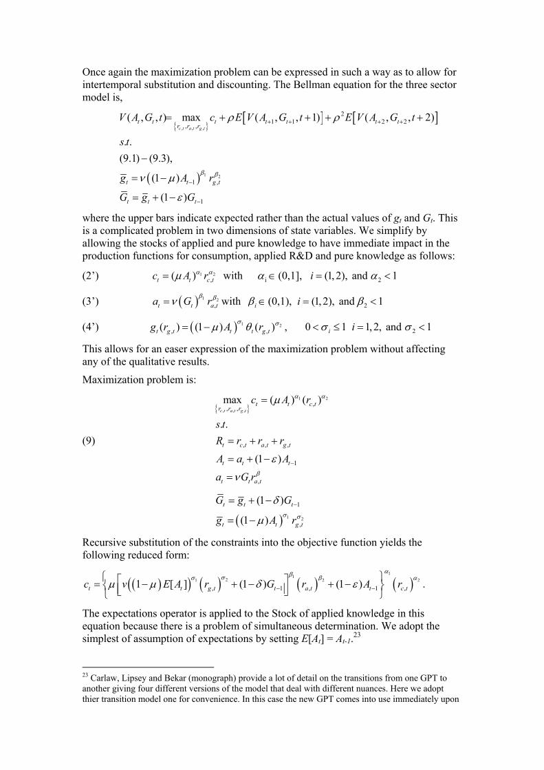
Once again the maximization problem can be expressed in such a way as to allow for intertemporal substitution and discounting. The Bellman equation for the three sector model is,
{ }[ ] [ ]
( )
, , ,
1 2
21 1 2 2
, ,
1 ,
1
( , , ) max ( , , 1) ( , , 2)
. .) (9.3),
(1 )
(1 )
c t a t g tt t t t t t t
r r r
t t g t
t t t
V A G t c E V A G t E V A G t
s t
g A r
G g G
β β
ρ ρ
ν µ
ε
+ + + +
−
−
= + + +
−
= −
= + −
(9.1
+
2c t
where the upper bars indicate expected rather than the actual values of gt and Gt. This is a complicated problem in two dimensions of state variables. We simplify by allowing the stocks of applied and pure knowledge to have immediate impact in the production functions for consumption, applied R&D and pure knowledge as follows:
(2’) 1,( )t tc A rα αµ= with i 2(0,1], (1, 2), and 1iα α∈ = <
(3’) ( ) 1 2,t ta G rβ
a tβν= with 2(0,1), (1, 2), and 1i iβ β∈ = <
(4’) ( ) 1 2, ,( ) (1 ) ( )t g t t t g tg r A rσ σµ θ= − , 20 1 1,2, and 1i iσ σ< ≤ = <
This allows for an easer expression of the maximization problem without affecting any of the qualitative results.
Maximization problem is:
(9)
{ }1 2
, , ,,
, ,
, , ,
1
,
max ( ) ( )
. .
(1 )
c t a t g tt t c t
r r r
t c t a t g t
t t t
t t a t
c A r
s tR r r r
A a A
a G r
α α
β
µ
ε
ν−
=
= + +
= + −
=
( ) 1 2
1
,
(1 )
(1 )t t t
t t
G g G
g A σg trσ
δ
µ−= + −
= −
Recursive substitution of the constraints into the objective function yields the following reduced form:
( )( ) ( ) ( ) ( )1
12 2 21
, 1 , 11 [ ] (1 ) (1 )t t g t t a t tc v E A r G r A rαβσ
,c tβ ασ
µ µ δ ε− − = − + − + −
.
The expectations operator is applied to the Stock of applied knowledge in this equation because there is a problem of simultaneous determination. We adopt the simplest of assumption of expectations by setting E[At] = At-1.23
23 Carlaw, Lipsey and Bekar (monograph) provide a lot of detail on the transitions from one GPT to another giving four different versions of the model that deal with different nuances. Here we adopt thier transition model one for convenience. In this case the new GPT comes into use immediately upon

3.2 Model of Structural Adjustment A new GPT may be well or poorly adapted to the existing facilitating structure.24 Typically real resources must be invested in substantial adjustments to many of the elements of the structure to accommodate the new GPT.25
We begin with the simplifying assumption that all of the structural adjustments takes place in the applied R&D sector, which we justify on two grounds. The first is simplicity. Having the structural adjustment in one sector is sufficient to demonstrate the qualitative outcomes. The second is that many of the actual structural adjustment problems do occur in the application of the GPT to various uses (e.g., the application of electricity to factories required a new organizational technology as well as several innovations in the applications of electricity to machines and tools).
Much of the previous model is preserved when economic structure is explicitly included. Equations 2 and 4-9 are unaltered. The resource constraint is altered to reflect the fact that resources must be allocated among four instead of the original three lines of activity:
(10) , , ,t c t a t g t s,tR r r r r= + + +
Where, rs, is the resource allocated to structural adjustment. This adjustment is assumed to have effect only in the applied R&D sector. As with the previous model, the arrival of a new GPT increases Gt in equations (11). However, the arrival of the new GPT comes with a structural adjustment cost SAt (equation 12) below, which reduces the immediate impact of the new GPT.
(11) ( ) 13 2
,
1
( )( ) ( )
(1 )t t t a
t t t
a v G SA r
A a A
ββt
βχ
ε −
=
= + − with 2(0,1), (1,2), and 1i iβ β∈ = < .
Where [0,1]χ ∈ allows only a portion of realised pure knowledge to influence applied R&D. (We make this assumption to simplify the forthcoming total factor productivity calculations.) SAt is defined as follows:
(12) tt
t
SSC
=SA .
This is a decreasing function of the total impact of the new GPT, defined as SCt (equation 13), and an increasing function of the structural adjustment effort, St, that accumulates from the point that the GPT arrives (equation 14).
(13) ( )
1( ) ( )1
s s z
s s z
t th
t t t tt teSC SC SC SC
e
τ γ
τ γ
+ −
−+ −
= + − +
( )1h ht t t tG Gψ −= − h
SC .
it arrival regardless of it productivity enhancing effects in the applied R&D sector relative to the old GPT. 24 This observation is made by a number of historians and students of technological change such as David (1990), Freeman and Perez (1988), Freeman and Louca (2001), Perez (2002), Lipsey and Bekar (1995) Lipsey, Bekar and Carlaw (1998b), and Carlaw, Lipsey and Bekar (manuscript). 25 Although we do not introduce labour explicitly in the model, we note that these structural adjustment costs can be sever when the arriving GPT causes big dislocations by separating significant numbers of workers from there work when an old technology is made obsolete.

SCt is the cost of structural adjustment defined as a function of the total impact of the new GPT, which we model by taking the difference between the total value of the new GPT relative to the old and a random variable ψt drawn from a Beta distribution. The structural adjustment costs are assumed to follow a logistic diffusion process similar to the GPT itself. So that as the GPT has a bigger impact it creates more structural adjustment costs. However, in order to match the empirical observations that structural adjustment costs are up front and productivity benefits of GPTs are occur later made in earlier chapters we assume that γs > γ τs < τ so that the structural adjustment impacts occur more quickly than the productivity diffusion of the GPT.
St is the accumulated effort to adapt structure to a new GPT.
(14) 1(1 )t t t tS s S φ−= + − ,
where
( ) ,(1 )t tGχ= − s trs , and
if *
0 otherwiset
ς λ λφ
≥=
,
st is the output flow of structural adjustment and (1-χ) is the proportion of pure knowledge that influences the productivity of resources in structural adjustment. st is dependent on the amount of resources devoted to producing adjustment in structure, rs,t, and a portion of the stock of useful pure knowledge, (1 - χ) Gt. This last assumption is made to ensure that resources devoted to producing structural adjustment increase in productivity at a rate similar to resources in all other lines of production in the system.
The two key sources of structural adjustment costs observed when a new GPT arrives, the new investment in structure that the new GPT requires due to its new complementarities with its many new applications and the amount of the old structure that is rendered useless by the new GPT are modelled as random variables. This is done to reflect the uncertainty about their size from GPT to GPT. The first random variable, ψt, conditions SCh
t reflecting the amount of new investment in structure that is required due to the novelty of the technology and its complementarities with new applications. The second random variable, φt depreciates or makes obsolete the previously accumulated investments in structure measured as the stock, St. During the life of an incumbent GPT, φt is zero and upon the arrival of the new GPT, φt is a random variable between 0 and 1 chosen from a uniform distribution. This implies that some of the structure that was adjusted to the existing GPT is not useful in facilitating the new GPT.
(15) [ ]( | , ) , 0 2t c cs beta x sψ ν η= < <
The constant sc allows the random variable drawn from the beta distribution to take on values larger than one. This, combined with the calibration of ν and η, determines the probability that ψt is greater than or less than one. ς is drawn from a Uniform distribution with support of [0, 1].
The maximization problem includes the allocation of resources to structural adjustment as follows:

(16) { }
1 2
, , , ,,
, , ,
, , , ,
max ( ) ( )
. .c t a t g t s t
t t c tr r r r
t c t a t g t s t
c A r
s tR r r r r
α αµ=
= + + +
( ) 13 2
,
1
( )( ) ( )
(1 )t t t a
t t t
G SA r
A a A
ββta v βχ
ε −
=
= + −
( ) 1 2
1
,
(1 )
(1 )t t t
t t
G g G
g A σg trσ
δ
µ−= + −
= −
and equations 12 – 15
3.3 Simulation of the model The model is solved using numerical simulation which requires calibrating parameter values. We choose values in order to achieve long run average growth rates of approximately 2% and GPT arrival rates of on average 30-35 periods. The qualitative results are robust to a wide rage of parameter values that meet the restriction specified in the model.
Table 3.1: Model parameters
Baseline three sector model
The parameter values chosen for this simulation are illustrative of a wide rage of possible values that meet our assumptions. We have tested a wide range of these values to ensure the robustness of the qualitative results.
α1 = 1 α1 = 0.34 β1 = 1 β2 = 0.34
σ1 = 1 σ2 = 0.34 v = 1 A0 = 1
G0 = 1 R = rc,t + ra,t + rg,t= 1000 ε = 0.01 δ = 0.01
γ = 0.06 τ = -6 µ = 0.5
For λ we choose ν = 5 and η = 10. The threshold value of λ* = 0.64. For ϑ we choose ν = 10, η = 5 and s = 1. As stated in the text θt is a random variable distributed uniformly with support [0.8, 1.2], mean 1, and variance (0.4)2/12.
Structural adjustment, four sector model
The parameterization for the model of structural adjustment is the same as the baseline model with the following additions.
χ = 0.8 R = rc,t + ra,t + rg,t + rs,t = 1000 β3 = 0.85
γs = 0.08 τs = -8
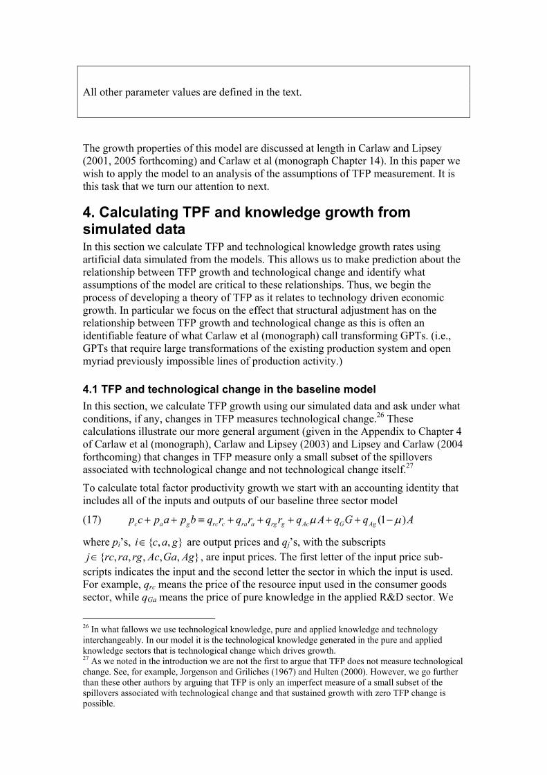
All other parameter values are defined in the text.
The growth properties of this model are discussed at length in Carlaw and Lipsey (2001, 2005 forthcoming) and Carlaw et al (monograph Chapter 14). In this paper we
is
ledge growth from
te TFP and technological knowledge growth rates using rom the models. This allows us to make prediction about the
ic
e., open
odel d ask under what These
law (2004
tity that includes all of the inputs and outputs of our baseline three sector model
)
wish to apply the model to an analysis of the assumptions of TFP measurement. It this task that we turn our attention to next.
4. Calculating TPF and knowsimulated data In this section we calculaartificial data simulated frelationship between TFP growth and technological change and identify what assumptions of the model are critical to these relationships. Thus, we begin the process of developing a theory of TFP as it relates to technology driven economgrowth. In particular we focus on the effect that structural adjustment has on therelationship between TFP growth and technological change as this is often an identifiable feature of what Carlaw et al (monograph) call transforming GPTs. (i.GPTs that require large transformations of the existing production system and myriad previously impossible lines of production activity.)
4.1 TFP and technological change in the baseline mIn this section, we calculate TFP growth using our simulated data anconditions, if any, changes in TFP measures technological change.26
calculations illustrate our more general argument (given in the Appendix to Chapter 4 of Carlaw et al (monograph), Carlaw and Lipsey (2003) and Lipsey and Carforthcoming) that changes in TFP measure only a small subset of the spillovers associated with technological change and not technological change itself.27
To calculate total factor productivity growth we start with an accounting iden
(17) (1c a g rc c ra a rg g Ac G Agp c p a p b q r q r q r q A q G q Aµ µ+ + ≡ + + + + + −
t price sub-d.
where pi’s, { , , }i c a g∈ are output prices and qj’s, with the subscripts { , , }j rc ra r Ag∈ , are input prices. The first letter of the inpu
scripts indicates the input and the second letter the sector in which the input is userc e price of the resource input used in the consumer goods
sector, while qGa means the price of pure knowledge in the applied R&D sector. We
, , ,g Ac Ga
ple, q meansFor exam th
26 In what fallows we use technological knowledge, pure and applied knowledge and technology interchangeably. In our model it is the technological knowledge generated in the pure and applied knowledge sectors that is technological change which drives growth. 27 As we noted in the introduction we are not the first to argue that TFP does not measure technological change. See, for example, Jorgenson and Griliches (1967) and Hulten (2000). However, we go further than these other authors by arguing that TFP is only an imperfect measure of a small subset of the spillovers associated with technological change and that sustained growth with zero TFP change is possible.
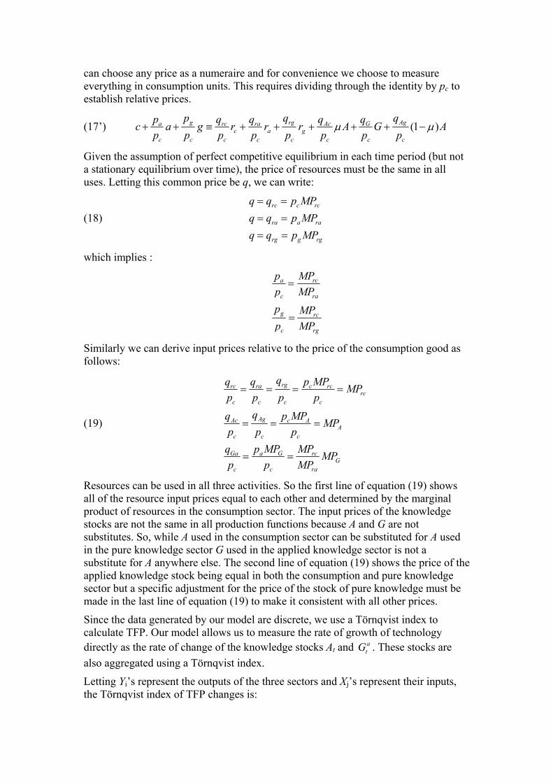
can choose any price as a numeraire and for convenience we choose to measure everything in consumption units. This requires dividing through the identity by pc to establish relative prices.
(17’) ga p q qp q q q qc a+ + (1 )rg Arc ra Ac Gc a g
c c c c c c c c
g r r r A Gp p p p p p p p
µ µ≡ + + + + + −
sumption of perfect competitive equilibrium in each time period (but not Given the as
g A
a stationary equilibrium over time), the price of resources must be the same in all
(18)
uses. Letting this common price be q, we can write:
rc c rcq q p MP= =
ra a ra
rg g rg
q q p MPq q p MP= =
= =
which implies :
a r
c r
g rc
c r
p MPp MPp MP
=
=
c
a
g
p MP
Similarly we can derive input prices relative to the price of the consumption good as follows:
(19)
rgrc ra c rcrc
c c c c
AgAc c AA
c c c
Ga a G rcG
c c ra
MPp p p p
qq p MP MPp p p
q p MP MP MPp p MP
= = = =
= = =
= =
ctivities. So the first line of
qq q p MP
Resources can be used in all three a equation (19) shows all of the resource input prices equal to each other and determined by the marginal
d
edge
re
ree sectors and Xj’s represent their inputs,
product of resources in the consumption sector. The input prices of the knowledge stocks are not the same in all production functions because A and G are not substitutes. So, while A used in the consumption sector can be substituted for A usein the pure knowledge sector G used in the applied knowledge sector is not asubstitute for A anywhere else. The second line of equation (19) shows the price of theapplied knowledge stock being equal in both the consumption and pure knowlsector but a specific adjustment for the price of the stock of pure knowledge must be made in the last line of equation (19) to make it consistent with all other prices.
Since the data generated by our model are discrete, we use a Törnqvist index to calculate TFP. Our model allows us to measure the rate of growth of technologydirectly as the rate of change of the knowledge stocks At and a
tG . These stocks aalso aggregated using a Törnqvist index.
Letting Yi’s represent the outputs of the ththe Törnqvist index of TFP changes is:
(20) [ ] [1ln( ) ln( ) ln( ) ln(t t t tTFP Y Y X−∆ = − − − ]
[ ] [1
, , 1 1 , , 1 1
)
0.5( ) ln( ) ln( ) 0.5( ) ln( ) ln( )t
i t i t t t j t j t t ti i
X
w w Y Y v v X X−
− − −= + − − + −∑ ∑ ]−
Measuring TFP and knowledge growth for the individual sectors is straight forward in our framework since we know the exact specifications of the production functions. So, for example, TFP change in the consumption sector is measured as:
(21) [ ]1 1 1 2 , , 1ln( ) ln( ) ln( ) ln( ) ln( ) ln( )t t t t t c t c tTFPc c c A A r rα α ∆ = − − − − − − − −
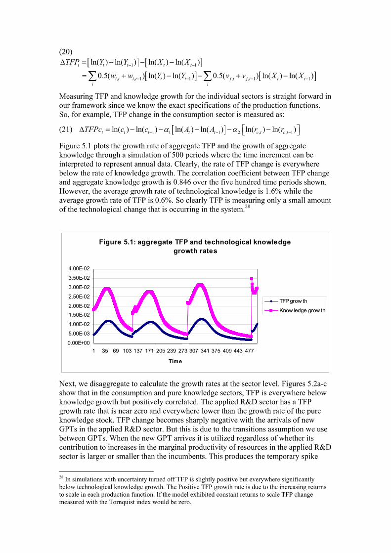
Figureknowle
5.1 plots the growth rate of aggregate TFP and the growth of aggregate dge through a simulation of 500 periods where the time increment can be
ere nge
.
interpreted to represent annual data. Clearly, the rate of TFP change is everywhbelow the rate of knowledge growth. The correlation coefficient between TFP chaand aggregate knowledge growth is 0.846 over the five hundred time periods shownHowever, the average growth rate of technological knowledge is 1.6% while the average growth rate of TFP is 0.6%. So clearly TFP is measuring only a small amount of the technological change that is occurring in the system.28
Figure 5.1: aggregate TFP and technological knowledge growth rates
0.00E+00
5.00E-03
1.00E-02
1.50E-022.00E-02
2.50E-02
3.00E-02
3.50E-02
4.00E-02
1 35 69 103 137 171 205 239 273 307 341 375 409 443 477
Time
TFP grow th
Know ledge grow th
Next, we disaggregate to calculate the growth rates at the sector level. Figures 5.2a-c show that in the consumption and pure knowledge sectors, TFP is everywhere below
knowledge growth but positively correlated. The applied R&D sector has a TFP growth rate that is near zero and everywhere lower than the growth rate of the pure knowledge stock. TFP change becomes sharply negative with the arrivals of new GPTs in the applied R&D sector. But this is due to the transitions assumption we usebetween GPTs. When the new GPT arrives it is utilized regardless of whether its contribution to increases in the marginal productivity of resources in the applied R&Dsector is larger or smaller than the incumbents. This produces the temporary spike
28 In simulations with uncertainty turned off TFP is slightly positive but everywhere significantly below technological knowledge growth. The Positive TFP growth rate is due to the increasing returns to scale in each production function. If the model exhibited constant returns to scale TFP change measured with the Tornquist index would be zero.

downward. Because of are assumption that each GPT arrives in a crude from and diffuses logistically the probability that the new GPTs contribution is lower than inthe incumbents is high. Alternative transition assumptions remove this spike.
Figure 5.2a: consumption sector TFP and
technological knowledge growth rates
0.00E+00
1.00E-02
2.00E-02
3.00E-02
4.00E-02
5.00E-02
1 36 71 106 141 176 211 246 281 316 351 386 421 456 491
Time
TFP growth
Knowledge growth
Figure 5.2b: Applied R&D sector TFP and technological knowledge growth rates
-2.00E-01-1.50E-01-1.00E-01-5.00E-020.00E+005.00E-021.00E-011.50E-012.00E-01
1 40 79 118 157 196 235 274 313 352 391 430 469
Time
TFP growth
Knowledge growth
Figure 5.3c: Pure knowledge sector TFP and technological knowledge growth rates
-1.00E-02
0.00E+00
1.00E-02
2.00E-02
3.00E-02
4.00E-02
5.00E-02
1 35 69 103 137 171 20 23 27 30 341 37 40 44 47
Ti me
TFP growt h
Knowledge growt h
Alternative simulation runs provide different realization of the random variables and thus different quantitative results. However, Figures 5.1 and 5.2 illustrate the general
in each sector rather than the share weights of the Törnqvist
qualitative results.29
If the actual exponential parameters of the individual production functions are used to calculate TFP growthindex, each sectors TFP growth is zero while the growth technological knowledge is positive. Using the Törnqvist index to aggregate yields a positive aggregate TFP
29 Carlaw (2004) provides a sensitivity analysis of the results and demonstrates that TFP does not measure technological change by reducing the amount of variability in the system, making the probability of an arrival of a GPT in each period equal to one. In all cases TFP growth is everywhere significantly below the growth rate of technological knowledge. The reason that TFP is positive at all in the system is because the parameterizations used in the simulations are such that all lines of production have increasing returns to scale and the Törnqvist index number aggregation method use imposes share weights that imply constant returns to scale.
growth rate. This is not meant to be an argument that the Törnqvist is an inappropriateaggregation method in fact it might be argued that allowing the procedure to detecincreasing returns to scale is appropriate. What is does indicate is that if TFP growth rate numbers are interpreted to measure changes in technological change, the interpretation is wrong. In all cases we have technological change. But what the Törnqvist index is detecting is the increasing returns to scale of the system nottechnological change per se.
5.2 TFP and technological
t
change in the structural adjustment model We now include all of the inputs and outputs of our four sector structural adjustment model in the accounting identity.
(22) p c p a p b p s+ + +
( ) ( ) ( ) ( )(1 ) (1 )a g s
rc c ra a rg g rs s Ac Ga Gs Ag Asq r q r q r q r q A q G q G q A q SAµ χ χ µ≡ + + + + + + − + − +
where once again pi’s, { , , , }i c a g s∈ are output prices and qj’s, with the subscripts { , , , , , , , , }
c
j rc ra rg rs Ac Ga Gs Ag As∈ , are input prices. Note that we include SA as an t
input rather than just S b the ratio of St to SCt that matters in the producti divide through the identity by pc to establish
relative prices.
(22’)pp
t ecause it is on function for applied R&D. Again we
( ) ( ) (1 ) (1 )
ga s
c c c
rg Agrc ra rs Ac Ga Gs Sc a g
c c c c c c c c c
pa g sp p
q qq q q q q q qr r r rs A G G Ap p p p p p p p P
µ χ χ µ
+ +
≡ + + + + + + − + − +
cp
+
In
SA
put prices are established as in the previous case:
(23)
rc c rq q p MP= = c
ra a ra
rg g rg
rs s rs
q q p MPq q p MP
p MPq q
= =
= =
= =
which implies:
a r
c r
g rc
c r
c
a
g
s rc
c rs
p MPp MPp MPp MP
p MPp MP
=
=
=
Similarly we can derive input prices relative to the price of the consumption good as follows:

(24)
rgrc ra rs c rcrc
c c c c c
AgAc c AA
c c c
Ga a Ga rcGa
c c ra
S s s rcS
c c rs
qq q q p MP MPp p p p p
qq p MP MPp p p
q p MP MP MPp p MP
q p MP MP MPp p MP
= = = = =
= = =
= =
= =
Resources can be used in all four activities. So, the first line of equation (24) shows all of the resource input prices equal to each other and determined by the marginal product of resources in the consumption sector. The input prices of the knowledge stocks are not the same in all production functions because A, G and S are not substitutes. So, while A used in the consumption sector can be substituted for A used in the pure knowledge sector G and S used in the applied knowledge sector are not a substitutes for A anywhere else.
Again, we use a Törnqvist index to calculate TFP and to aggregate the knowledge stocks. The sector specific TFP growth rates are again calculated directly from the production functions.
In the present model, there are four outputs, four resource inputs, four knowledge inputs and a stock of structural adjustment input. Technological knowledge comprises the four stocks of knowledge which are just the accumulated flows of output from the pure and applied research sectors divided among the four production activities. These are aggregated using a Tornquist index. We assume that the stock of accumulated structural adjustment is not included in aggregate knowledge for this illustration, though it is arguable that it should be included. When we do include investment in structural adjustment as knowledge it strengthens the result that TFP change is either unrelated or negatively related to technological knowledge growth.
Figure 5.9 plots the growth rates of aggregate TFP and knowledge. TFP is now negatively correlated with knowledge growth. The correlation coefficient between the two rates of change is -0.82. When a GPT arrives, the TFP growth rate drops and in many cases becomes negative for several periods. Furthermore, as some GPTs mature TFP growth increase and over estimates actual technological change. The implication is that when new GPTs require adjustments in the facilitating structure, changes in measured TFP will slow down even though actual technological change is accelerating over several periods. In the case shown, a maximum of 4.6 percent (an average of 1.8 percent) of the economy’s total resources are allocated to structural adjustment. Yet, this small resource cost has significant implications for TFP growth rates and their interpretation as measures of technological change. A small diversion of resources out of other productive activities into the activity of structural adjustment can cause significant drops in the TFP growth rate (in some cases the rate becomes negative).
Furthermore, our results are consistent with the kind of “New Economy” productivity bonus experienced in the USA from the mid 1990 into the new Millennium. However, our theory predicts that the productivity bonus coincides with a technological knowledge growth rate slow down, at least in the model as we have specified it.

Figure 5.9: aggregate TFP and technological knowledge growth rates
-2.00E-01
-1.50E-01
-1.00E-01
-5.00E-02
0.00E+00
5.00E-02
1.00E-01
1.50E-01
2.00E-01
1 34 67 100 133 166 199 232 265 298 331 364 397 430 463 496
Time
TFP grow th
Know ledge grow th
Next, we disaggregate to calculate TFP sector by sector. Figures 5.10a-d show the TFP change and the growth rate of the knowledge stock that goes into production in each sector. In all but the applied R&D case TFP change is positive and positively correlated with, but everywhere below the growth rate of knowledge in that sector. TFP change is negatively correlated with knowledge growth in the applied R&D sector and negative when GPTs arrive.
Figure 5.10a: consumption sector TFP and technological knowledge growth rates
0.00E+00
1.00E-02
2.00E-02
3.00E-02
4.00E-02
5.00E-02
6.00E-02
1 38 75 112 149 186 223 260 297 334 371 408 445 482
Time
TFP growth
Knowledge growth
Figure 5.10b: Applied R&D sector TFP and technological knowledge growth rates
-5.00E-02
0.00E+00
5.00E-02
1.00E-01
1.50E-01
1 38 75 112 149 186 223 260 297 334 371 408 445 482
Time
TFP growth
Knowledge growth

Figure 5.10c: Pure knowledge sector TFP and technological knowledge growth rates
-1.00E-02
0.00E+00
1.00E-02
2.00E-02
3.00E-02
4.00E-02
5.00E-02
6.00E-02
1 38 75 112 149 186 223 260 297 334 371 408 445 482
Time
TFP growth
Knowledge growth
Figure 5.10d: Pure knowledge sector TFP and technological knowledge growth rates
-5.00E-02
0.00E+00
5.00E-02
1.00E-01
1.50E-01
2.00E-01
1 40 79 118 157 196 23 27 313 35 391 43 46
Ti me
TFP growt h
Knowledge growt h
Once again it can be shown that if the exponential parameter values in each line of production in the system are used to calculate TFP, then the TFP growth rates are very close to zero in each sector and become slightly negatively correlated with TFP in some sectors.
The analysis demonstrates that TFP growth does not reflect technological change, at least within the framework. What TFP growth does reflect is the increasing returns to scale in the production functions of the system. Also what is clear is that in the aggregate sufficiently high structural adjustment costs cause TFP growth to become strongly negatively correlated with technological change which manifests in the model as knowledge growth.
It should also be noted that our aggregate is artificial in the sense that we have one consumption sector, two knowledge producing sectors and in the second model an additional structural adjustment sector. In reality it is often the case that all of these production activities take place with in a given measured sector in the national accounts. For example, the steam engine was invented by the mining sector and spread in its application to many other sectors of the first industrial revolution economies. What we have called the applied R&D and structural adjustment sectors certainly exist as components of the industrial sectors measured in the national accounts of most economies.30 For example, in the sectors of the New Zealand economy that we examine in the next section, applications of ICT are being undertaken by firms within the sectors for which data is reported. Firms within these sectors are adopting ICT technologies and adapting it to their needs, through a process of costly investment and internal innovation. In this sense the results that our simulated aggregate TFP calculation is generating are most appropriately interpreted to reflect the kind of TFP calculation we should expect to see in each of the industries in the New Zealand data examined in the next section.
30 It is debatable whether pure knowledge is more appropriately treated as a separate sector in today’s world of science based bio-technology and nano-technology driven primary research.

One further note of qualification is required. The model and simulation exercise is one where there is only ever one GPT operating in the system at any moment in time. In contrast, real economies comprise several GPTs, all at different stages in their own logistic diffusions, and which all affect the system in myriad interrelated ways. For examples, Australia is currently experiencing the rapid diffusion of ICT along side applications of lasers and made to order materials. It is continuing to experience the impact of electricity through an ever increasing development of applications for this power GPT. There are many other examples that could be noted but this suffices to make the point. All of these technologies have influences on the measures of performance even at the disaggregated industry level discussed in the next section. Furthermore, these different technologies have different impacts in these different industries or sectors.
Carlaw, et al (monograph chapter 14) provide the algebra to suggest that a model of multiple GPTs is possible within their framework, but to date it has not been implemented in a computer simulation. However, the framework developed here provides for the possibility of a quick-and-dirty multiple GPT simulation. If we aggregate data from the baseline model and the structural adjustment model to calculate TFP growth and knowledge growth we find that a number of possibilities emerge.31 Depending on the realizations of the random variables in each model the correlation between TFP growth and knowledge growth becomes less negative and less significant. In some cases the correlation is not significantly different from zero. This simulated result comes closer to some of the empirical results we observe in the next section. But, until the complete formal model has been constructed and a proper calibration made for each measured sector or industry under analysis, nothing more than casual inference can be made. Thus, a note of caution is warranted when interpreting the statistical results derived from the forthcoming section. These cannot be viewed as supporting evidence for the theory and simulation of the GPT model is warranted. The empirical analysis is consistent with the theory but does not constitute a rigorous test of it.
The empirical analysis is an indication that TFP growth is not measuring technological change and the model and simulation analysis suggest an avenue of investigation as to why that might be the case. Furthermore, the model if judged to be appropriate begins to offer a theoretical interpretation of TFP that is at least consistent with observed productivity slowdowns and a sometimes negative contemporaneous correlation between TFP growth and technological change.
4. New Zealand ICT Diffusion and Productivity The contributions of embodied technological change to TFP growth have been studied in the growth accounting literature. Hulten (1992) and Jorgenson (1966) have focused on the measurement of the efficiency of the capital stock and the effects of measurement errors on productivity estimates. These authors argue that quality change (or Investment Specific Technological (IST) change growth) is difficult to observe, and therefore may not be measured accurately in the National Income and Product Accounts (NIPA). In order to obtain an estimate of the size of error associate with the official capital stock estimates, Hulten used quality-corrected data from
31 The aggregation was done by taking crude averages of the growth rate of TFP and knowledge. A more sophisticated analysis requires the fully integrated computer simulation code suggested in the Carlaw, Lipsey and Bekar (monograph) multiple model.

Gordon (1990). Gordon found that the official deflators for producer durable equipment overstate quality-corrected inflation in capital goods, and therefore understate increases in capital input.
Following Greenwood et al (1997 and 2000), Carlaw and Kosempel (2004) adopt a computable general equilibrium approach to measuring changes in the quality of investment in Canada. They demonstrate that IST made important contributions to Canadian output growth during the 1961-96 period. One of the key results that they establish is that IST is negatively correlated with TFP particularly since 1974.
IST is calculated by making the unrealistic assumption that the economy, sector or industry under examination in is a perfectly competitive general equilibrium which has become characterized as the Ramsey-Cass-Koopmans model following the pioneering work of Ramsey (1928) Cass (1965) and Koopmans (1965). In this framework the microeconomic decisions of consumers determine the saving rates, levels of consumption and stocks of capital in the economy whose aggregate production capacity is characterised by a constant returns to scale production function defined over capital and labour.32
Within such a framework constant income share weights but an increasing capital to labour ratio can only be reconciled by an increasing quality of capital, which is the result that Carlaw and Kosempel (2004) verify empirically. In their analysis the measure of residual neutral technological change, which would be equal to TFP in the absence of increases in investment quality, is negative over much of the period from 1974 onward. They interpret this negative measure to potentially indicate a structural adjustment cost associated with the adoption of the new technology implicit in the high quality capital investments of the sort discussed by David (1990) and Lipsey, Bekar and Carlaw (1998b). We return to this issue latter in the paper when we discuss the industry level Australian data.
We report here some of our follow up analysis of changes in investment quality and changes in TFP in 16 OECD countries (where comparable data was available) reveals that the negative relationship between IST and TFP change appeared in most of the countries in the data set. The data span the period 1970 to 1997, although the times serries are not as long for some countries included in the analysis. Correlations and their significance are calculated by linearly regressing TFP growth on IST growth. This simple procedure allows for easy calculation of correlation and the statistical significance of the correlation between the two rates of change, however, it also has some obviously flawed assumptions in that it is unlikely that the relationship between TFP and IST growth is linear. We use it because reveals that there is clearly something wrong with TFP as a contemporaneous measure of technological change.
Table 4.1
Correlation Significance Ave. TFP growth Ave. IST growth Australia -0.2003968 -1.625798274 0.005659614 0.030617859
32 It is important to note that the assumption of constant returns to scale is a very strong one and one on which the entire calculation depends. In the absence of constant returns to scale it is not clear that IST is solely a measure of investment quality. We maintain the assumption here and use the measure as being indicative of the point that TFP does not measure changes in technology even though our independent measure of technological change, IST, is itself likely imperfect.

Austria 0.08229683 0.797660716 0.006229159 0.014620765 Canada -0.0352858 -0.45167094 0.004854536 0.066904922 Germany -0.9011252 -1.908711555 0.002441211 0.01003906 Denmark 0.05655763 0.486804643 0.006646929 0.013692764 Spain -0.1684784 -1.193274005 0.007006918 0.017480885 Finland -0.355621 -1.485503129 0.009873589 0.00124906 France 0.0950263 0.664095684 0.008940826 0.022266437 United Kingdom -0.3561123 -3.451808317 0.008177637 0.011128314 Greece -0.1231186 -2.570949582 0.000862841 0.025734561 Ireland -0.0474524 -0.350604117 0.015489796 0.017249422 Italy -0.029527 -0.184041154 0.005292738 0.010806238 Japan 0.42931646 2.932067842 0.009564838 0.039670992 Netherlands 0.29245471 2.300423326 -1.94774E-05 0.01748624 New Zealand -0.2171726 -1.299822494 -0.00088776 0.049056889 Sweden 0.06241575 0.559180659 0.003969073 0.020516658
The results shown in Table 4.1 indicate that the relationship between TFP and IST is week. In most cases there is a negative relationship, in two cases a significant one. Only in two cases is there a significant positive relationship. Given the assumptions necessary to make these calculations we do not draw any strong conclusions. But we take this as weak evidence that there is no relationship between our independent measure of technological change and TFP growth. There is possibly a negative relationship over the period examined at least for some economies.
In addition to the empirical evidence on investment quality we are able to track ICT diffusion in New Zealand proximately, over a relatively short time horizon by looking at the diffusion of mobile telephones, internet domains, web sites and internet uses in the economy.
Figure 4.1: ICT Diffusion in New Zealand
0
0.5
1
1.5
2
2.5
3
1988
1989
1990
1991
1992
1993
1994
1995
1996
1997
1998
1999
2000
2001
2002
Mobile phonesInternet domainsWeb sitesInternet users

Figure 4.1 shows the levels of use of mobile phones, Internet domains, web sites and Internet users in New Zealand during the period 1988-2002.33 The data have a logistic looking diffusion pattern. Unfortunately not all of the series cover the whole period. For example, the number of web sites only runs from 1998 to 2002. In spite of the limited data we are able to do some analysis that goes some way toward testing the hypotheses that emerge from the traditional and non-traditional views.
The traditional view argues that technological change is contemporaneously correlated with productivity change. The non-traditional view argues that technological change will be either uncorrelated or negatively contemporaneously correlated with productivity change. It also argues that productivity change will understate technological change.
Figure 4.2: Growth rates of TFP and diffusion rates
-0.5
0
0.5
1
1.5
2
1989
1990
1991
1992
1993
1994
1995
1996
1997
1998
1999
2000
2001
2002
Primary
Mining and quarying
Construction
Manufacturing
Mobile phone diffusion
Internet Domains
Web sites
Internet users
Figure 4.3: Growth rates of TFP and diffusion rates
-0.2
0
0.2
0.4
0.6
0.8
1
1.2
1.4
1.6
1.8
1989
1990
1991
1992
1993
1994
1995
1996
1997
1998
1999
2000
2001
2002
Electricity, water and gas
Transport andComunicationBusiness and propertyservicesPersonal and communityservicesRetail and wholesale trade
Mobile phone diffusion
Internet domains
Web sites
Internet users
Figures 4.2 and 4.3 show the rates of TFP change and diffusion rates for the nine industrial sectors of New Zealand and the four measures of diffusion. The diffusion
33 The data on ICT diffusion comes from the New Zealand Ministry of Economic Development’s report titled Statistics on Information Technology in New Zealand: Updated to 2003: URL http://www.med.govt.nz/pbt/infotech/it-stats/it-stats-2003/.

rates are all above the TFP growth rates. This is consistent with the non-traditional views argument that TFP is not a measure of the rate of technological change.
To test the hypothesis that TFP change is contemporaneously correlated with technological change we linearly regress TFP growth on the diffusion rate of mobile telephones in New Zealand. We choose only mobile telephones because it is the longest time series we have, allowing for the best statistical result. Table 4.1 reports correlation coefficients and t statistics as well average growth rates of TFP for each industry.
Table 4.2 SECTOR Correlation Significance Ave. TFP growth Ave. diffusion rate
Primary 0.00 -0.08 0.01 0.51 Mining and Quarrying -0.09 -1.19 0.00 0.51
Construction 0.00 0.08 -0.02 0.51 Manufacturing 0.02 0.74 0.00 0.51
Electricity, gas and water 0.05 1.44 0.00 0.51 Transport and communications 0.03 1.36 0.06 0.51 Business and property services -0.03 -1.49 0.00 0.51
Personal and community services 0.00 0.13 0.01 0.51 Retail and wholesale trade 0.01 0.65 0.01 0.51
The critical value of the one tailed test with a 95% level of confidence and 13 degrees of freedom is 2.16. In all cases we have a failure to reject the null hypothesis that the coefficient is significantly different from zero.
5. Conclusions We set out in paper to analyse two views of technology diffusion in the context of ICT diffusion in New Zealand. In doing so, we begin the development of a theory of MFP or TFP by developing a multi-sector model of endogenous GPT-driven growth. The need for such a theory arrises out of the mutually incompatible interpretations of the measures technological and productivity change. Such a need also arrises out of the inconsistency in the interpretation of TFP growth as a measure of technological change when compared to other independent measures of technological change such as IST. The two different measures appear to be uncorrelated or even negatively correlated.
To begin the process of developing a theory of TFP we build two models of GPT-driven growth – a basic three sector model and a four sector model that includes structural adjustment costs – based on the historical and theoretical research of Carlaw and Lipsey (monograph), as well as, a cruder earlier versions of the three sector model (Carlaw and Lipsey (2001 and 2005)). In the models, a sequence of GPTs arrive each at uncertain times and with uncertain productive impacts that diffuse according to a logistic process. The models assume behaviour that results in resource allocations such that a non-stationary equilibrium is generated. The model has the property that in the absence of future GPTs there are diminishing returns and growth asymptotically approaches zero. But the arrival of new GPTs rejuvenates the growth process.
Because this model requires a numerical solution procedure that is iterated through several periods it provides a ready opportunity for Monte Carlo analysis of the assumptions that underlay both endogenous growth modelling and TFP growth calculations. We do such and exercise here and confirm the arguments of Carlaw and

Lipsey (2003) and Lipsey and Carlaw (2004) and Carlaw (2004) that TFP is not a measure of technological change. We find that while under some conditions TFP is positively correlated with direct and independent measures of technological change it persistently under estimates such technological change. Under other conditions, such as structural adjustment to accommodate a new GPT, TPF growth is negatively correlated with measured technological change and persistently underestimates technological change when a new GPT arrives and overestimates technological change as the GPT matures. In both model TFP fails detect the arrival of GPTs appropriately (i.e., as big technological shocks).
The findings in the IST empirical analysis and the simple empirical analysis of the New Zealand ICT diffusion data are consistent with the view that ICT is a major new transforming GPT that generates the kind of structural adjustment costs discussed in Lipsey, Bekar and Carlaw (1998b) and Carlaw et al (Monograph). However, all of these empirical findings have to be viewed with a critical eye because there are a number of assumptions necessary to interpret the measures of technological change as being valid. Although, they do have the property that they are independent measures of technological change and therefore provide some basis of comparison and testing of the various interpretations of TFP growth, they are limited in terms of the number of observations. Thus, very limited inference can be drawn. They point in a common direction. TFP does not measure technological change. Furthermore, it may be negatively correlated with technological change when that change is driven by a transforming GPT such as ICT, which is something that the theory predicts. What the results suggest is that further research is warranted. In particular more attention must be paid to collecting independent measures of technological change and more research need to be done to develop a theory of technological change and economic growth.

Bibliography Abramovitz, M. (1956) ‘Resource and Output Trends in the U.S. Since 1870,’ American Economic Review, 46, 5-23.
Aghion, P. and P. Howitt (1998), “On the Macroeconomic Effects of Major Technological Change”, in E. Helpman (ed), General Purpose Technologies and Economic Growth, (Cambridge: MIT Press), 121-144.
Aghion, P. and P. Howitt (1992), “A Model of Growth Through Creative Destruction”, Econometrica, 60, 232-396.
Baily, M.N., (2002) “Macroeconomic Implications of the New Economy,” Institute for International Economics Working paper, 2002.
Bresnahan, T. and Trajtenberg, E. (1992) “General Purpose Technologies: Engines of Economic Growth?” NBER Working Paper No. 4148.
Carlaw, K. I. (2004) “ICT in Australian Economic Performance: An Investigation of the Assumptions Influencing Productivity Estimates” paper to be presented to the Asia Pacific Productivity Conference, Brisbane, 14-16 July 2004, Invited paper Plenary Session #2: Productivity Growth and ICT. Carlaw, K. I., R. G. Lipsey and C. Bekar, Economic Transformations: General Purpose Technologies and Long Term Economic Growth, monograph in preparation.
Carlaw, K. I. and R. G. Lipsey (2005 forthcoming) “GPT-Driven, Endogenous Growth with Uncorrelated Changes in TFP”, Paper presented to the Modeling and Simulation Society of Australia and New Zealand International Congress MODSIM 2003, in Townsville, Australia, forthcoming in Mathematics and Computers in Simulation.
Carlaw, K. I. and S. Kosempel (2004) “The sources of total factor productivity growth: Evidence from Canadian data” Economics of Innovation and New Technology, 13(4), 299-309.
Carlaw, Kenneth I. and R. G. Lipsey (2003) “Productivity, Technology and Economic Growth: What is the relationship?” Journal of Economic Surveys, 17(3).
Carlaw, K. I. and R. G. Lipsey (2002) ‘Externalities, Technological Complementarities and Sustained Economic Growth,’ Research Policy, 31 (8-9), 1305-1315.
Carlaw, Kenneth I. and Richard G. Lipsey (2001), ‘Externalities versus Technological Complementarities: a model of GPT-driven, sustained growth’, A Paper Presented at The Conference in Honour of the 20th Anniversary of Nelson and Winter’s Book An Evolutionary Theory Of Economic Change, Aalborg Denmark, 12-15 June 2001.
Cass, D. (1965) “Optimum Growth in an Aggregate Model of Capital Accumulation” Review of Economic Studies, 32, 233-240.
David, P. and G. Wright (1999) “General Purpose Technologies and Surges in Productivity: Historical Reflections on the Future of the ICT Revolution”, University of Oxford Discussion papers in Economic and Social History, Number 31.

David. P. (1990) “The Dynamo and the Computer: An Historical Perspective on the Modern Productivity Paradox” American Economic Review, 80(2), 355-61.
Freeman, C. and C. Perez (1988) “Structural Crises of Adjustment, Business Cycles and Investment Behaviour,” in Dosi, G. et al (eds.) Technical change and economic theory, (London and New York: Pinter; distributed by Columbia University Press, New York), 38-66.
Freeman, Chris and F. Louca (2001) As Time Goes By: From the Industrial Revolution to the Information Revolution, (Oxford: Oxford University Press).
Gordon, R. J. (1990) “The measurement of durable goods prices,” National Bureau of Economic Research Monograph series Chicago and London: University of Chicago Press.
Gordon, R.J., (2000) “Does the ‘New Economy’ Measure up to the Great Inventions of the Past?,” Journal of Economic Perspectives, 14(4), 49-74.
Greenwood, J., Z. Hercowitz and P. Krusell. (1997). “Long Run Implications of Investment-Specific Technological Change,” American Economic Review 87(3), 342-62.
Greenwood, J., Z. Hercowitz and P. Krusell. (2000). “The Role of Investment-Specific Technological Change in the Business Cycle,” European Economic Review 44(1), 91-115.
Griliches, Z. (1994), “Productivity, R&D, and the Data Constraint”, AER, 84(1).
Helpman, Elhanan, (ed) (1998) General Purpose Technologies and Economic Growth, (Cambridge: MIT Press).
Helpman, E. and M. Trajtenberg (1998a), “A Time to Sow and a Time to Reap” in E. Helpman (ed), General Purpose Technologies and Economic Growth, (Cambridge: MIT Press), 55-84.
Helpman, E. and M. Trajtenberg (1998b), Diffusion of General Purpose Technologies, in E. Helpman (ed), General Purpose Technologies and Economic Growth, (Cambridge: MIT Press), 85-119.
Howitt, P. (1998) “Measurement, Obsolescence, and General Purpose Technologies”, in E. Helpman ed. (1998) General Purpose Technologies and Economic Growth, MIT Press: Massachusetts, 219 – 251.
Hulten, C. R. (1992). “Growth Accounting when Technological Change is Embodied in Capital,” American Economic Review, 82(4), 964-980.
Hulten, C. R. (2000) ‘Total Factor Productivity: A Short Biography,’ NBER Working Paper, 7471, (Washington: National Bureau of Economic Research).
Jorgenson, D.W. (1966). “The Embodiment Hypothesis,” Journal of Political Economy, 74(1), 1-17.
Jorgensen, D. and Z. Griliches (1967) ‘The Explanation of Productivity Change,’ Review of Economic Studies, 34, 249-83.
Koopmans, T. C. (1965) “On the Concept of Optimal Economic Growth” in The Economic Approach to Development Planning (Amsterdam: Elsevier).
Krugman, Paul (1996) ‘The Myth of Asia’s Miracle,’ in Pop Internationalism (Cambridge: MIT Press).

Lipsey, R. G., C. Bekar and K. I. Carlaw (1998a) ‘What Requires Explanation,’ Chapter 2 in Helpman (1998).
Lipsey, R. G., C. Bekar and K. I. Carlaw (1988b) ‘The Consequences of Changes in GPTs,’ Chapter 7 in Helpman (1998).
Lipsey, R. G. and K. I. Carlaw (2004) “Total Factor Productivity And The Measurement Of Technological Change”, forthcoming in the Canadian Journal of Economics.
Lucas, R. E. (1988) “On the Mechanics of Economic Development,” Journal of Monetary Economics, 22(1), 3-42.
Nelson, R. R. (1964) ‘Aggregate Production Function and Medium-Range Growth Projections,’ American Economic Review, 54, 575-606.
Perez, C. (2002) Technological Revolutions and Financial Capital, (Cheltenham, UK: Edward Elgar).
Ramsey, F. P. (1928) “A Mathematical Theory of Saving” Economic Journal, 38, 543-559.
Romer, P. (1986) “Increasing Returns and Long-run Growth,” Journal of Political Economy, 94(5),1002-37.
Rymes, Thomas K., (1971) On Concepts of Capital and Technical Change, (Cambridge: Cambridge University Press).
Solow, R. (1956) ‘A Contribution to the Theory of Economic Growth,’ Quarterly Journal of Economics, 70, 65-94.
Solow, R. (1987) “We’d Better Watch out,” New York Times Book Review, pp. 36.
Triplett, J.E. 'Economic Statistics, the New Economy, and the Productivity Slowdown' Business Economics, 34(2), 1999, pp. 13-17.
Young, A. (1992) ‘A Tale of Two Cities: Factor Accumulation and Technical Change in Hong Kong and Singapore,’ NBER Macroeconomic Annual, (Cambridge: MIT press).