ices report 12-15 isogeometric divergence-conforming b

ICES REPORT 12-15

April 2012

Isogeometric Divergence-conforming B-splines for theSteady Navier-Stokes Equations

by

John A. Evans and Thomas J.R. Hughes

The Institute for Computational Engineering and SciencesThe University of Texas at AustinAustin, Texas 78712

Reference: John A. Evans and Thomas J.R. Hughes, Isogeometric Divergence-conforming B-splines for theSteady Navier-Stokes Equations, ICES REPORT 12-15, The Institute for Computational Engineering andSciences, The University of Texas at Austin, April 2012.

Isogeometric Divergence-conforming B-splinesfor the Steady Navier-Stokes Equations

John A. Evans a,* and Thomas J.R. Hughes a

a Institute for Computational Engineering and Sciences, The University of Texas at Austin,∗ Corresponding author. E-mail address: [email protected]

Abstract

We develop divergence-conforming B-spline discretizations for the numerical solu-tion of the steady Navier-Stokes equations. These discretizations are motivated bythe recent theory of isogeometric discrete differential forms and may be interpretedas smooth generalizations of Raviart-Thomas elements. They are (at least) patch-wise C0 and can be directly utilized in the Galerkin solution of steady Navier-Stokesflow for single-patch configurations. When applied to incompressible flows, these dis-cretizations produce pointwise divergence-free velocity fields and hence exactly satisfymass conservation. Consequently, discrete variational formulations employing the newdiscretization scheme are automatically momentum-conservative and energy-stable.In the presence of no-slip boundary conditions and multi-patch geometries, the dis-continuous Galerkin framework is invoked to enforce tangential continuity withoutupsetting the conservation or stability properties of the method across patch bound-aries. Furthermore, as no-slip boundary conditions are enforced weakly, the methodautomatically defaults to a compatible discretization of Euler flow in the limit ofvanishing viscosity. The proposed discretizations are extended to general mapped ge-ometries using divergence-preserving transformations. For sufficiently regular single-patch solutions subject to a smallness condition, we prove a priori error estimateswhich are optimal for the discrete velocity field and suboptimal, by one order, for thediscrete pressure field. We present a comprehensive suite of numerical experimentswhich indicate optimal convergence rates for both the discrete velocity and pressurefields for general configurations, suggesting that our a priori estimates may be conser-vative. These numerical experiments also suggest our discretization methodology isrobust with respect to Reynolds number and more accurate than classical numericalmethods for the steady Navier-Stokes equations.

Keywords: Steady Navier-Stokes equations, B-splines, Isogeometric analysis, Divergence-conforming discretizations

1

1 Introduction

Steady Navier-Stokes flow is an important simplification of fully unsteady Navier-Stokes flow. Many low speed, laminar fluid flows may be accurately described bythe steady Navier-Stokes equations. Additionally, one arrives at a steady Navier-Stokes problem by conducting a Reynolds time-averaging of statistically stationaryNavier-Stokes flows (see Chapters 3 and 4 of [31]). Despite its simple appearance,the steady Navier-Stokes problem has presented considerable difficulty in its numer-ical approximation. It is subject to the Babuska-Brezzi inf-sup condition, and whenthe convection operator is expressed in conservation form and the incompressibilityconstraint is not met exactly, terms corresponding to convection can actually accreteenergy. This ultimately leads to unstable numerical formulations, and alternative rep-resentations of the convection operator have been devised to bypass this instability.The most popular of these in the finite element community is the skew-symmetricrepresentation [40]. Discretizations of the convection term using the skew-symmetricrepresentation neither produce nor dissipate energy and hence lead to stable numer-ical methods. Unfortunately, these discretizations do not inherit the conservationstructure of the Navier-Stokes equations. Alternatively, provably stable, convergent,and locally-conservative discontinuous Galerkin discretizations have been devised forthe steady Navier-Stokes equations in [11, 12], but these discretizations are encum-bered with a proliferation of degrees of freedom and are thus largely limited to twospatial dimensions. Hybrid technologies have recently been proposed with the aim ofextending the applicability of discontinuous Galerkin methods to larger problem sizes[28, 29].

Another discretization procedure for the steady Navier-Stokes equations arisesthrough the intelligent choice of weighting function in a Petrov-Galerkin method. Apopular method of choice is the use of an advective formulation in conjunction withthe Streamline-Upwind Petrov-Galerkin (SUPG) method [7] to handle convective in-stabilities and the Pressure-Stabilizing Petrov-Galerkin (PSPG) method [25, 37] tohandle pressure instabilities. Unfortunately, the theoretical analysis of this methodin the steady regime has been entirely restricted to linearized Oseen problems wherethe convection velocity is assumed fixed and divergence-free. These linearized modelproblems are ultimately insufficient as the discrete convection velocity is not, in gen-eral, divergence-free. To further control the divergence term, so-called grad-div stabi-lization techniques [33] have been proposed which add artificial dilatational stressesto the underlying variational formulation. Using a combination of an advective for-mulation, SUPG, PSPG, and grad-div stabilization, provably convergent numericalmethods have been devised for the steady Navier-Stokes equations (see Chapter 3of [33]), and such methods can be made to globally conserve momentum through aresidual-based modification [26]. Still, a provably convergent H1-Galerkin finite ele-ment discretization of the three-dimensional steady Navier-Stokes equations writtenin conservation form has proved elusive.

2

In this paper, we present divergence-conforming B-spline discretizations for thesteady Navier-Stokes problem. These discretizations are motivated by the theory ofisogeometric discrete differential forms [9, 10] and extend the Darcy-Stokes-Brinkmandiscretizations presented in [19] to nonlinear Navier-Stokes flows. As our discretiza-tions return pointwise divergence-free velocity fields, we can utilize a variational for-mulation written in conservation form without being susceptible to instability. Weimpose no-penetration boundary conditions strongly and no-slip boundary conditionsweakly using Nitsche’s method. This allows our discretization procedure to naturallydefault to a conforming approximation of Euler flow in the limit of vanishing vis-cosity. This also allows our method to capture boundary layers without resortingto stretched meshes [3, 4]. We prove stability and error estimates for single-patchdiscretizations under a smallness condition. Our error estimates are optimal for thediscrete velocity field and suboptimal, by one order, for the discrete pressure fieldprovided that that the exact solution is sufficiently regular. All of our estimates’ de-pendencies on the viscosity and the penalty parameter of Nitsche’s method are madeexplicit in our analysis. We utilize the methods of exact and manufactured solutionsto verify our error estimates and find our discrete pressure fields converge at optimalorder in contrast with our theoretical estimates. We further test the effectiveness ofour method by considering the application of our discretization to the analysis of twobenchmark problems: lid-driven cavity flow and confined jet impingement.

An outline of this paper is as follows. In the following section, we present somebasic notation. In Section 3, we recall the steady Navier-Stokes problem subject tohomogeneous Dirichlet boundary conditions. In Section 4, we briefly review B-splines,the basic building blocks of our new discretization technique, and in Section 5, wedefine the B-spline spaces which we will utilize to discretize velocity and pressurefields. In Section 6, we present our discrete variational formulation for the steadyNavier-Stokes problem and prove continuity, stability, and a priori error estimatesfor the single-patch setting. In Section 7, we discuss the extension of our methodologyto the multi-patch setting. In Sections 8 and 9, we present numerical results, and inSection 10, we draw conclusions. Before proceeding, note that one might say there isa fundamental issue concerning the fact that our analysis only covers flows subject to“small data”. However, well-posedness of the continuous problem is subject to a sim-ilar constraint, and we believe the small data assumption is natural as medium- andlarge-Reynolds number flows are inherently unsteady in both laminar and turbulentregimes.

2 Notation

We begin this paper with some basic notation. For d a positive integer representingdimension, let D ⊂ Rd denote an arbitrary bounded Lipschitz domain with boundary∂D. As usual, let L2(D) denote the space of square integrable functions on D and

3

define L2(D) = (L2(D))d. We will also utilize the more general Lebesgue spaces

Lp(D) where 1 ≤ p ≤ ∞ and their vectorial counterparts Lp(D). Let Hk(D) denotethe space of functions in L2(D) whose kth-order derivatives belong to L2(D) and

define Hk(D) =(Hk(D)

)d. We identify with Hk(D) the standard Sobolev norm

‖v‖Hk(D) =

∑|α|<k

‖Dαv‖2L2(D)

1/2

where α = (α1, α2, . . . , αd) is a multi-index of non-negative integers, |α| = α1 + α2 +. . .+ αd, and

Dα =∂|α|

∂xα11 ∂x

α22 . . . ∂xαdd

.

We denote the Sobolev semi-norms as |·|Hk(D), and we adopt the convention H0(D) =L2(D). Throughout, Sobolev spaces of fractional order are defined using functionspace interpolation (see, e.g., Chapter 1 of [38]). We define H1

0 (D) ⊂ H1(D) to bethe subspace of functions with homogeneous boundary conditions and define H1

0(D)to be the vectorial counterpart of H1

0 (D). We define Hs(div;D) to be the Sobolevspace of all functions in Hs(Ω) whose divergence also belongs to Hs(D). This spaceis equipped with the norm

‖v‖Hs(div;D) =(‖v‖2

Hs(D) + ‖divv‖2Hs(D)

)1/2.

When s = 0, we omit the superscript. We also define

H0(div;D) = v ∈ H(div;D) : v · n = 0 on ∂D

where n denotes the outward pointing unit normal. Finally, we denote L20(D) ⊂ L2(D)

as the space of square-integrable functions with zero average on D.

3 The Steady Navier-Stokes Problem

In this section, we recall the steady Navier-Stokes problem subject to homogeneousDirichlet boundary conditions. For d a positive integer, let Ω denote a Lipschitzbounded open set of Rd. Throughout this paper, d will be either 2 or 3. The problemof interest is as follows.

(S)

Given ν ∈ R+ and f : Ω → Rd, find u : Ω → Rd and p : Ω → R suchthat

∇ · (u⊗ u)−∇ · (2ν∇su) + gradp = f in Ω (1)

divu = 0 in Ω (2)

u = 0 on ∂Ω. (3)

4

Above, u denotes the flow velocity of a fluid moving through the domain Ω, p de-notes the pressure acting on the fluid divided by the fluid density, ν denotes thekinematic viscosity of the fluid, f denotes a body force acting on the fluid divided bythe density, and ∇su denotes the symmetrized gradient of the velocity field defined

by ∇su = 12

(∇u + (∇u)T

). Note that the pressure is only determined up to an

arbitrary constant.Assuming that f ∈ L2(Ω) , the weak form for the steady Navier-Stokes problem is

written as follows:

(W )

Find u ∈ H10(Ω) and p ∈ L2

0(Ω) such that

k(u,v) + c(u,u; v)− b(p,v) + b(q,u) = (f,v)L2(Ω) (4)

for all v ∈ H10(Ω) and q ∈ L2

0(Ω) where

k(w,v) = (2ν∇sw,∇sv)(L2(Ω))d×d , ∀w,v ∈ H10(Ω) , (5)

b(q,v) = (q, divv)L2(Ω) , ∀q ∈ L20(Ω),v ∈ H1

0(Ω) , (6)

c(w,x; v) = − (w ⊗ x,∇v)(L2(Ω))d×d , ∀w,x,v ∈ H10(Ω) . (7)

Note that the trilinear form c(·, ·; ·) : H10(Ω)×H1

0(Ω)×H10(Ω) → R makes sense due

to the continuous Sobolev embedding

H10(Ω) → L4(Ω). (8)

In fact, as ∂Ω is Lipschitz, we have the stronger embedding H1(Ω) → L4(Ω).We have the following existence and uniqueness theorem for flows subject to small

data whose proof may be found in [22].

Theorem 3.1. Problem (W ) has a unique weak solution (u, p) ∈ H10(Ω) × L2

0(Ω)provided the problem data satisfies an inequality of the form

CΩCPoinν2

‖f‖L2(Ω) < 1 (9)

where CΩ is a constant which only depends on Ω and CPoin is the positive constantappearing in Poincare’s inequality:

‖v‖H1(Ω) ≤ CPoin|v|H1(Ω), ∀v ∈ H1(Ω) ∩ H0(div; Ω) . (10)

Furthermore, such a weak solution satisfies the inequality

|u|H1(Ω) ≤CPoinν‖f‖L2(Ω). (11)

5

Remark 3.1. Note that, since ν is constant and divu = 0,

∇ · (2ν∇su) = ν∆u. (12)

This inspires a different variational formulation than that presented here which isoften the basis for numerical discretization (see, for example, [12]). However, such aformulation cannot easily accommodate traction boundary conditions. We have foundthat discrete formulations based on either of the diffusion operators given by (12) yieldqualitatively and quantitatively similar results.

Remark 3.2. In general, we may replace the constant-viscosity Newtonian stresstensor given here, T = 2ν∇su, with more suitable choices of stress tensor. Ouranalysis does not cover this general setting.

4 B-splines and Geometrical Mappings

In this section, we briefly introduce B-splines, the primary ingredient in our discretiza-tion technique for the steady Navier-Stokes equations. We also introduce mappingswhich will allow us to extend our discretization technique to general geometries ofengineering interest. For an overview of B-splines, their properties, and robust algo-rithms for evaluating their values and derivatives, see de Boor [14] and Schumaker[35]. For the application of B-splines to finite element analysis, see Hollig [23] andCottrell, Hughes, and Bazilevs [13].

4.1 Univariate B-splines

For two positive integers k and n, representing degree and dimensionality respectively,let us introduce the ordered knot vector

Ξ := 0 = ξ1, ξ2, . . . , ξn+k+1 = 1 (13)

whereξ1 ≤ ξ2 ≤ . . . ξn+k+1.

Given Ξ and k, univariate B-spline basis functions are constructed recursively startingwith piecewise constants (k = 0):

B0i (ξ) =

1 if ξi ≤ ξ < ξi+1

0 otherwise.(14)

For k = 1, 2, 3, . . ., they are defined by

Bki (ξ) =

ξ − ξiξi+k − ξi

Bk−1i (ξ) +

ξi+k+1 − ξξi+k+1 − ξi+1

Bk−1i+1 (ξ). (15)

6

When ξi+k − ξi = 0, ξ−ξiξi+k−ξi

is taken to be zero, and similarly, when ξi+k+1− ξi+1 = 0,ξi+k+1−ξ

ξi+k+1−ξi+1is taken to be zero. B-spline basis functions are piecewise polynomials of

degree k, form a partition of unity, have local support, and are non-negative. Werefer to linear combinations of B-spline basis functions as B-splines or simply splines.

Let us now introduce the vector ζ = ζ1, . . . , ζm of knots without repetitions anda corresponding vector r1, . . . , rm of knot multiplicities. That is, ri is defined to bethe multiplicity of the knot ζi in Ξ. We assume that ri ≤ k+1. Let us further assumethroughout that r1 = rm = k + 1, i.e, that Ξ is an open knot vector. This allowsus to easily prescribe Dirichlet boundary conditions. At the point ζi, B-spline basisfunctions have αj := k− rj continuous derivatives. We define the regularity vector αby α := α1, . . . , αm. By construction, α1 = αm = −1. In what follows, we utilizethe notation

|α| = minαi : 2 ≤ i ≤ m− 1 (16)

and α− 1 := −1, α2 − 1, . . . , αm−1 − 1,−1 when αi ≥ 0 for 2 ≤ i ≤ m− 1.We denote the space of B-splines spanned by the basis functions Bk

i as

Skα := spanBki

ni=1

. (17)

When k ≥ 1 and αi ≥ 0 for 2 ≤ i ≤ m − 1, the derivatives of functions in Skα aresplines as well. In fact, we have the stronger relationship

d

dxv : v ∈ Skα

≡ Sk−1

α−1 . (18)

One of the most important properties of univariate B-splines is refinement and, per-haps more importantly, nestedness of refinement. Knot insertion and degree elevationalgorithms are described in detail in Chapter 2 of [13].

4.2 Multivariate B-splines

The definition of multivariate B-splines follows easily through a tensor-product con-struction. For d again a positive integer, let us consider the unit cube Ω = (0, 1)d ⊂Rd, which we will henceforth refer to as the parametric domain. Mimicking the one-dimensional case, given integers kl and nl for l = 1, . . . , d, let us introduce openknot vectors Ξl = ξ1,l, . . . , ξnl+kl+1,l and the associated vectors ζl = ζ1,l, . . . , ζml,l,r1,l, . . . , rml,l, and αl = α1,l, . . . , αml,l. There is a parametric Cartesian meshMh

associated with these knot vectors partitioning the parametric domain into rectangu-lar parallelepipeds. Visually,

Mh = Q = ⊗l=1,...,d (ζil,l, ζil+1,l) , 1 ≤ il ≤ ml − 1 . (19)

For each element Q ∈ Mh we associate a parametric mesh size hQ = diam(Q). Wealso define a shape regularity constant λ which satisfies the inequality

λ−1 ≤ hQ,min

hQ≤ λ, ∀Q ∈Mh, (20)

7

where hQ,min denotes the length of the smallest edge of Q. A sequence of parametricmeshes that satisfy the above inequality for an identical shape regularity constant issaid to be locally quasi-uniform.

We associate with each knot vector Ξl (l = 1, . . . , d) univariate B-spline basisfunctions Bkl

il,lof degree kl for il = 1, . . . , nl. On the mesh Mh, we define the tensor-

product B-spline basis functions as

Bk1,...,kdi1,...,id

:= Bk1i1,1⊗ . . .⊗Bkd

id,d, i1 = 1, . . . , n1, . . . id = 1, . . . , nd. (21)

We then accordingly define the tensor-product B-spline space as

Sk1,...,kdα1,...,αd≡ Sk1,...,kdα1,...,αd

(Mh) := spanBk1,...,kdi1,...,id

n1,...,nd

i1=1,...,id=1. (22)

Like their univariate counterparts, multivariate B-spline basis functions are piece-wise polynomial, form a partition of unity, have local support, and are non-negative.Defining the regularity constant

α := minl=1,...,d

min2≤il≤ml−1

αil,l (23)

we see that our B-splines are Cα-continuous throughout the domain Ω. Refinement ofmultivariate B-spline bases is obtained by applying knot insertion and degree elevationin tensor-product fashion. In the remainder of the text, we consider a family ofnested meshes Mhh≤h0 and associated B-spline spaces

Sk1,...,kdα1,...,αd

(Mh)h≤h0

that

have been obtained by successive applications of knot refinement. Furthermore, weassume throughout that the mesh family Mhh≤h0 is locally quasi-uniform.

Note that each element Q = ⊗l=1,...,d (ζil,l, ζil+1,l) has the equivalent representationQ = ⊗l=1,...,d (ξjl,l, ξjl+1,l) for some index jl. With this in mind, we associate with eachelement a support extension Q, defined as

Q := ⊗l=1,...,d (ξjl−kl,l, ξjl+kl+1,l) . (24)

The support extension is the interior of the set formed by the union of the supportsof all B-spline basis functions whose support intersects Q. Note that each elementbelongs to the support extension of at most Πl=1,...,d(2kl + 1) elements.

4.3 Piecewise Smooth Functions, Geometrical Mappings, andPhysical Mesh Entities

On the parametric meshMh, we define the space of piecewise smooth functions withinterelement regularity given by the vectors α1, . . . ,αd as

C∞α1,...,αd= C∞α1,...,αd

(Mh) . (25)

8

Precisely, a function in C∞α1,...,αdis a function whose restriction to an element Q ∈Mh

admits a C∞ extension in the closure of that element and which has αil,l contin-uous derivatives with respect to the lth coordinate along the internal mesh faces(x1, . . . , xd) : xl = ζil,l, ζjl′ ,l′ < xl′ < ζjl′+1,l

′ , l′ 6= l for all il = 2, . . . ,ml − 1 andjl′ = 1, . . . ,ml′ − 1. Note immediately that any function lying in the B-spline spaceSk1,...,kdα1,...,αd

also lies in C∞α1,...,αd.

Unless specified otherwise, we assume throughout the rest of the paper that thephysical domain Ω ⊂ Rd can be exactly parametrized by a geometrical mapping

F : Ω → Ω belonging to(C∞α1,...,αd

)dwith piecewise smooth inverse. We further

assume that the physical domain Ω is simply connected with connected boundary∂Ω and the geometrical mapping is independent of the mesh family index h. Ageometrical mapping meeting our criteria could be defined utilizing B-splines or Non-Uniform Rational B-Splines (NURBS) on the coarsest mesh Mh0 . For examples ofsuch mappings, see Chapter 2 of [13]. NURBS mappings are especially useful as theycan represent many geometries of scientific and engineering interest and are the maintools employed in Computer Aided Design (CAD) software. Later in this paper, wewill utilize a polar mapping to solve a flow problem on a cylindrical geometry. Thegeometrical mapping F naturally induces a mesh

Kh = K : K = F(Q), Q ∈Mh (26)

on the physical domain Ω. We define for each element K ∈ Kh a physical mesh size

hK = ‖DF‖L∞(Q)hQ (27)

where Q is the pre-image of K, and we also define the support extension K = F(Q).We define for a given mesh the global mesh size

h = max hK , K ∈ Kh .

Note that as the parametric mesh family Mhh≤h0 is locally quasi-uniform and thegeometrical mapping F is independent of the mesh family index h, the physical meshfamily Khh≤h0 is also locally quasi-uniform. We refer to the physical domain Ω and

its pre-image Ω interchangeably as the patch. It should be noted that, in general, thedomain Ω cannot be represented using just a single patch. Instead, multiple patchesmust be employed. We will discuss further the multi-patch setting in Section 7.

We define on the parametric mesh a set of mesh faces Fh = F where F is a faceof one or more elements in Mh. We define the physical set of mesh faces as

Fh = F = F(F ) : F ∈ Fh

and we define the boundary mesh to be

Γh = F ∈ Fh : F ⊂ ∂Ω .

9

By construction,∂Ω = ∪F∈ΓhF .

Note that for each face F ∈ Γh there is a unique K ∈ Kh such that F is a “face” ofK (in the sense that F is the image of a face of Q, the pre-image of K). We hencedefine for such a face the mesh size

hF := hK .

One may also define hF to be the wall-normal mesh-size as is done in [3]. Such adefinition is more appropriate when stretched meshes are utilized in the presence oflayers.

Throughout the paper, we will utilize the terminology “a constant independentof h”. When we employ such terminology, we simply indicate that the constantwill not depend on the given mesh and, in particular, its size. The constant may,however, depend on the domain, the shape regularity of the parametric mesh family,the polynomial degree and smoothness of the employed B-spline spaces, and global,mesh-invariant measures of the parametric mapping.

5 Discretization of Velocity and Pressure Fields

In this section, we define the B-spline spaces which we will utilize to discretize thevelocity and pressure fields appearing in the steady Navier-Stokes problem. Thesespaces are motivated by the recent theory of isogeometric discrete differential forms[9, 10] and may be interpreted as smooth generalizations of Raviart-Thomas elements[32]. We first define our discrete velocity and pressure spaces on the parametric

domain Ω = (0, 1)d and then define discrete spaces on the physical domain Ω usingdivergence- and integral-preserving transformations. We finish this section with apresentation of local approximation estimates and trace inequalities for our discretevelocity and pressure spaces. For a more in-depth discussion of the discrete velocityand pressure spaces used in this paper, see Section 5 of [19].

5.1 Discrete Spaces on the Parametric Domain

Using the notation of the previous section and assuming that

α := min|αl| : l = 1, . . . , d ≥ 1,

we define the following two spaces:

Vh :=

Sk1,k2−1α1,α2−1 × S

k1−1,k2α1−1,α2

if d = 2,

Sk1,k2−1,k3−1α1,α2−1,α3−1 × S

k1−1,k2,k3−1α1−1,α2,α3−1 × S

k1−1,k2−1,k3α1−1,α2−1,α3

if d = 3,

10

Qh :=

Sk1−1,k2−1α1−1,α2−1 if d = 2,

Sk1−1,k2−1,k3−1α1−1,α2−1,α3−1 if d = 3.

The space Vh comprises our set of discrete velocity fields while Qh comprises ourset of discrete pressure fields. Note that as α ≥ 1, our discrete velocity fields areH1-conforming. If we allow α = 0, our spaces collapse to standard Raviart-Thomasmixed finite elements [32]. In order to deal with no-penetration boundary conditions,we make use of the following constrained discrete spaces:

V0,h :=

vh ∈ Vh : vh · n = 0 on ∂Ω,

Q0,h :=

qh ∈ Qh :

∫Ω

qhdx = 0

.

Above, n denotes the outward-facing normal to ∂Ω. As specified in the introduction,we choose to enforce no-slip boundary conditions weakly using Nitsche’s method [30].

Due to the special relationship given by (18), the spaces V0,h and Q0,h along with theparametric divergence operator form the bounded discrete cochain complex

V0,hdiv−−−→ Q0,h

where div is the divergence operator on the unit cube Ω. In fact, we have a muchstronger result due to the results of [9].

Proposition 5.1. There exist L2-stable projection operators Π0Vh

: H0(div; Ω) → V0,h

and Π0Qh

: L20(Ω)→ Q0,h such that the following diagram commutes:

H0(div; Ω)div−−−→ L2

0(Ω)

Π0Vh

y Π0Qh

yV0,h

div−−−→ Q0,h.

(28)

Furthermore, there exists a positive constant Cu independent of h such that

‖Π0Vh

v‖H1(Ω) ≤ Cu‖v‖H1(Ω), ∀v ∈ H0(div; Ω) ∩ H1(Ω) . (29)

5.2 Discrete Spaces on the Physical Domain

To define our discrete velocity and pressure spaces on the physical domain, we intro-duce the following pullback operators:

ιu(v) := det (DF) (DF)−1 (v F) , v ∈ H0(div; Ω) (30)

ιp(q) := det (DF) (q F) , q ∈ L20(Ω) (31)

11

where DF is the Jacobian matrix of the parametric mapping F. The push-forwardgiven by (30), popularly known as the Piola transform, has two important properties:(i) it preserves the nullity of normal components, (ii) it maps divergences to diver-gences. On the other hand, the push-forward given by (31) has the property that itpreserves the nullity of the integral operator. Due to these properties, we have thefollowing commuting diagram:


0(Ω)

ιu

x ιp

xH0(div; Ω)

div−−−→ L20(Ω).

(32)

This motivates the use of the following discrete velocity and pressure spaces in thephysical domain:

V0,h :=

v ∈ H0(div; Ω) : ιu(v) ∈ V0,h

,

Q0,h :=q ∈ L2

0(Ω) : ιp(q) ∈ Q0,h

.

Furthermore, we define the projectors Π0Vh : H0(div; Ω) → V0,h and Π0

Qh : L2(Ω) →Q0,h via the compositions

Π0Qh := ι−1

u Π0Qh ιu, Π0

Qh := ι−1p Π0

Qh ιp.

Employing the preceding results and terminology as well as the smoothness propertiesof the parametric mapping F , we arrive at the following proposition.

Proposition 5.2. The following diagram commutes:


0(Ω)

Π0Vh

y Π0Qh

yV0,h

div−−−→ Q0,h.

(33)

Furthermore, there exists a positive constant Cu independent of h such that

‖Π0Vhv‖H1(Ω) ≤ Cu‖v‖H1(Ω), ∀v ∈ H0(div; Ω) ∩ H1(Ω) . (34)

We immediately have an inf-sup condition for our discrete velocity/pressure pair.

Proposition 5.3. There exists a positive constant β independent of h such that thefollowing holds: for every qh ∈ Q0,h, there exists a vh ∈ V0,h such that:

divvh = qh (35)

12

and‖vh‖H1(Ω) ≤ β−1‖qh‖L2(Ω). (36)

Hence,

infqh∈Q0,h

qh 6=0

supvh∈V0,h

(divvh, qh)L2(Ω)

‖vh‖H1(Ω)‖qh‖L2(Ω)

≥ β. (37)

Proof. See the proof of Proposition 5.3 in [19].

We also have the following result.

Proposition 5.4. If vh ∈ V0,h satisfies

(divvh, qh)L2(Ω) = 0, ∀qh ∈ Q0,h, (38)

then divvh ≡ 0.

Proof. The proof holds trivially as div maps V0,h onto Q0,h.

Hence, by choosing V0,h and Q0,h as discrete velocity and pressure spaces, wearrive at a discretization that automatically returns velocity fields that are pointwisedivergence-free.

5.3 Approximation Results and Trace Inequalities

Let us definek′ = min

l=1,...,d|kl − 1| . (39)

Note that the discrete velocity and pressure spaces V0,h and Q0,h consist of mappedpiecewise polynomials which are complete up to degree k′. Hence, k′ may be thoughtof as the polynomial degree of our discretization technique. The following resultdetails the local approximation properties of our discrete spaces. Its proof may befound in [9].

Proposition 5.5. Let K ∈ Kh and K denote the support extension of K. For0 ≤ j ≤ s ≤ k′ + 1, we have

|v− Π0Vhv|Hj(K) ≤ Chs−jK ‖v‖Hs(K), ∀v ∈ Hs(K) ∩ H0(div; Ω) (40)

|q − Π0Qh q|Hj(K) ≤ Chs−jK ‖q‖Hs(K), ∀q ∈ Hs(K) ∩ L2

0(Ω) (41)

where C denotes a positive constant, possibly different at each appearance, independentof h.

13

Hence, our discrete spaces deliver optimal rates of convergence from an approxi-mation point of view. We will also need the following trace estimate in our ensuingmathematical analysis. Its proof can be found in [16].

Proposition 5.6. Let K ∈ Kh and Q = F−1(K). Then we have

‖ (∇svh) n‖(L2(∂K))d ≤ Ctraceh−1K ‖vh‖H1(K), ∀vh ∈ V0,h (42)

where Ctrace denotes a positive constant independent of h.

In [18], it was shown that Proposition 5.6 holds for B-splines and parametric finiteelements with Ctrace ∼ (k′)2. However, our numerical experience has indicated thata corresponding global trace inequality holds with Ctrace ∼ k′ if B-splines of maximalcontinuity are utilized. This allows us to select a smaller penalty parameter whenemploying Nitsche’s method. As we will see in the next section, our convergenceestimates scale inversely with the square root of Nitsche’s penalty parameter. Hence,we want to select Nitsche’s penalty parameter as small as possible.

6 The Discretized Problem

In this section, we approximate the homogeneous steady Navier-Stokes problem usingthe discrete velocity and pressure spaces introduced in the previous section. We provecontinuity, stability, and a priori estimates for our discretization scheme in the singlepatch setting under a smallness condition, and we explicitly track all of our estimates’dependencies on the viscosity and Nitsche’s penalty parameter.

6.1 Variational Formulation

We begin this section by presenting a discrete variational formulation for the steadyNavier-Stokes problem. Since members of V0,h do not satisfy homogeneous tangentialDirichlet boundary conditions, we resort to Nitsche’s method to weakly enforce no-slipboundary conditions. Defining the bilinear form

kh(w,v) = k(w,v)−∑F∈Γh

∫F

2ν

(((∇sv) n) ·w + ((∇sw) n) · v− Cpen

hFw · v

)ds

(43)where Cpen ≥ 1 is a chosen positive penalty constant, our discrete formulation iswritten as follows.

(G)

Find uh ∈ V0,h and ph ∈ Q0,h such that

kh(uh,vh) + c(uh,uh; vh)− b(ph,vh) + b(qh,uh) = (f,vh)L2(Ω) (44)

for all vh ∈ V0,h, qh ∈ Q0,h.

We have the following lemma detailing the consistency of our numerical method.

14

Lemma 6.1. Suppose that (u, p) is a solution of (W ) satisfying the regularity con-dition u ∈ H3/2+ε(Ω) for some ε > 0. Then:

kh(u,vh) + c(u,u; vh)− b(p,vh) + b(qh,u) = (f ,vh)L2(Ω) (45)

for all vh ∈ V0,h and qh ∈ Q0,h.

Proof. We trivially haveb(qh,u) = 0, ∀qh ∈ Q0,h.

Now let vh ∈ V0,h. By the Sobolev trace theorem, the assumption u ∈ H3/2+ε(Ω)guarantees that (∇su) n is well-defined along ∂Ω and (∇su) n ∈ (L2(∂Ω))d. Hence,the quantity kh(u,vh) is well-defined. Utilizing integration by parts and the fact thatu satisfies homogeneous Dirichlet boundary conditions and vh satisfies homogeneousnormal Dirichlet boundary conditions, we have

kh(u,vh) + c(u,u; vh)− b(p,vh) =

∫Ω

(∇ · (u⊗ u)−∇ · (2ν∇su) + gradp) · vh

=

∫Ω

f · vh

= (f,vh)L2(Ω).

This completes the proof of the lemma.

We have the following relationship between the exact solution and a numericalsolution.

Corollary 6.1. Let (uh, ph) denote a solution of (G), and let (u, p) denote a solutionof (W ) satisfying the regularity condition u ∈ H3/2+ε(Ω) for some ε > 0. Then:

kh(u− uh,vh) + c(u,u,vh)− c(uh,uh,vh)−b(p− ph,vh) + b(qh,u− uh) = 0 (46)


Finally, by Proposition 5.4, we have the following lemma.

Lemma 6.2. Let (uh, ph) denote a solution of (G). Then:

divuh ≡ 0 (47)

Weak imposition of no-slip boundary conditions allows our methodology to defaultautomatically to a compatible discretization of Euler flow in the setting of vanishingviscosity. Moreover, for large Reynolds number flows, there is a sharp boundary layer

15

in the vicinity of walls. Utilzing Nitsche’s method allows us to account for these layersin a stable and consistent manner without having to directly resolve them [2, 3, 4]. Infact, Nitsche’s method can be interpreted as a variationally consistent wall model. Tobetter see this interpretation, let us formally rewrite our discrete variational equationsas∫

Ω

T : ∇svhdx−∑F∈Γh

∫F

Q · vhds + c(uh,uh; vh)− b(ph,vh) + b(qh,uh) = (f,vh)L2(Ω)

(48)where T is a symmetric tensor satisfying∫

Ω

T : Wdx =

∫Ω

2ν∇suh : Wdx−∑F∈Γh

∫F

2νuh · (Wn) ds

=

∫Ω

2νuh · divWdx (in the sense of distributions) (49)

for symmetric tensors W with well-defined normal trace and Q a vector satisfying

Q = 2ν

((∇suh) n− Cpen

huh

). (50)

Above, T is a weakly defined viscous stress tensor and Q is the resultant viscousboundary traction vector. In the event that the no-slip boundary condition is metexactly, we recover T ≡ 2ν∇suh and Q ≡ 2ν (∇suh) n. Otherwise, the definitionsof T and Q are changed accordingly. The tangential component of Q given by (50),denoted Qtang, and calculated as

Qtang = Q− (Q · n) n, (51)

is the effective wall shear stress vector.As the discrete velocity field satisfies the no-penetration boundary condition strongly,

the vector Q is equal to the discrete shear stress 2ν (∇suh) n plus an additional wallshear stress term Q+ in the direction tangent to the wall. Specifically, we have

Q+ = −u∗2 uh‖uh‖

(52)

where

u∗2 =2νCpen‖uh‖

h. (53)

For under-resolved flow simulations, the magnitude of (∇suh) n in the direction tan-gent to the wall is relatively small and, as such, the tangential component of Q isdominated by Q+. In this sense, Q+ becomes a model for the wall shear stress. Asthe mesh is refined and the flow is resolved, Q+ → 0. The above interpretation allows

16

us to design physically motivated penalty values for Nitsche’s penalty parameter. No-tably, u∗ may be interpreted as the friction velocity. By specifying the value of u∗

using Spalding’s law of the wall [36], we recover a standard wall model for under-resolved flow simulations. For more on this approach, see Section 3 of [3]. We recall,however, that the numerically inspired (53) produced results of the same quality asthe u∗ given by Spalding’s physically inspired law of the wall.

Remark 6.1. If we wish to impose non-homogeneous tangential Dirichlet (e.g., pre-scribed slip) boundary conditions, we must add the following expression to the righthand side of our discrete formulation:

fN(vh) =∑F∈Γh

∫F

2ν

(− ((∇svh) n) · uBC +

CpenhF

uBC · vh)ds (54)

where uBC is a prescribed vector function defined on ∂Ω. If we also wish to imposenon-homogeneous normal Dirichlet (e.g., prescribed penetration) boundary conditions,we must impose these strongly and add the following expression to the left hand sideof our discrete formulation:

cUW (uh,vh) =∑F∈Γh

∫F

(uBC · n)+ uh · vhds (55)

and the following expression to the right hand side of our discrete formulation:

fUW (vh) = −∑F∈Γh

∫F

(uBC · n)− uBC · vhds (56)

where

(uBC · n)+ =

uBC · n if uBC · n > 0

0 otherwise

and

(uBC · n)− =

uBC · n if uBC · n ≤ 0

0 otherwise.

These additional terms correspond to upwinding.

6.2 Well-Posedness for Small Data

We now prove that our discrete formulation is well-posed under a smallness condition.Our method of proof mimics that of the continuous problem (see Theorem 10.1.1 of[22]). To begin, let us define the following mesh-dependent norm:

‖v‖2h := |v|2H1(Ω) +

∑F∈Γh

hF‖ (∇sv) n‖2(L2(F ))d +

∑F∈Γh

CpenhF‖v‖2

(L2(F ))d . (57)

17

We will also denote

V0,h := vh ∈ V0,h : divvh = 0 = vh ∈ V0,h : b(qh,vh) = 0, ∀qh ∈ Q0,h .

To proceed, we need to call upon stability and continuity results that were proven in[19] for divergence-conforming B-spline discretizations of the Darcy-Stokes-Brinkmanequations. These results hinge upon two assumptions regarding the size of Cpen. First,in light of Proposition 5.6, we assume that

Cpen ≥ 4hKC2PoinCKorn

‖ (∇svh) n‖2(L2(∂K))d

‖vh‖2H1(K)

, ∀K ∈ Kh, vh ∈ V0,h (58)

where CPoin is the Poincare constant appearing in (10) and CKorn is the positiveconstant associated with the following Korn’s inequality [6]:

|w|2H1(Ω) ≤ CKorn

(‖∇sw‖2

(L2(Ω))d×d + |∂Ω|−1/(d−1)‖w‖2(L2(∂Ω))d

), ∀w ∈ H1(Ω) .

Second, we assume thatCpen ≥ 4h0|∂Ω|−1/(d−1) (59)

where h0 is the mesh size of the coarsest mesh K0 and |∂Ω| denotes the length of ∂Ω ford = 2 and the area of ∂Ω for d = 3. This second assumption is necessary as rotationmodes carry zero energy. Hence, weak boundary conditions are needed to control thesemodes in rotationally symmetric (or near rotationally symmetric) configurations. Assuch configurations are of significant engineering interest, we believe that any analysisresults should cover these situations. Note that a constant Cpen satisfying the aboveassumption need not depend on h or ν. Rather, it only needs to depend on thesize of the domain, the polynomial degree and smoothness of the discretization, theparametric shape regularity, and global, mesh-invariant measures of the parametricmapping.

Corollary 6.2. Assume (58) and (59) are satisfied. Then we have

kh(w,v) ≤ 2νCcont‖w‖h‖v‖h, ∀w,v ∈ V0,h ⊕(

H10(Ω) ∩H3/2+ε(Ω)

)(60)

b(p,v) ≤ ‖p‖L2(Ω)‖v‖h ∀p ∈ L20(Ω),v ∈ V0,h ⊕

(H1

0(Ω) ∩H3/2+ε(Ω))(61)

kh(wh,wh) ≥ 2νCcoerc‖wh‖2h, ∀wh ∈ V0,h (62)

where ε > 0 is an arbitrary positive number and Ccont and Ccoerc are positive constantswhich are independent of h, ν, Cpen, and ε. Furthermore, we have

infqh∈Q0,h,qh 6=0

supvh∈V0,h

(divvh, qh)

‖vh‖V(h)‖qh‖Q≥ β. (63)

where β is a positive constant independent of h and ν which asymptotically scalesinversely with the square root of Cpen.

18

We will also need the following two lemmas. The first lemma gives a Lipschitzcontinuity result for the trilinear form c(·, ·; ·). This result hinges upon Sobolev em-beddings which exist because our domain is Lipschitz. The second lemma gives asemi-coercivity result for the trilinear form c(·, ·; ·).

Lemma 6.3. There exists a constant C0 only dependent on Ω such that

c(w1,x; v)− c(w2,x; v) ≤ C0|w1 −w2|H1(Ω)|x|H1(Ω)|v|H1(Ω) (64)

for all w1,w2,x,v ∈ H1(Ω) ∩ H0(div; Ω).

Proof. Let w1,w2,x,v ∈ H1(Ω) ∩ H0(div; Ω) be arbitrary. Note that since ∂Ω isLipschitz, we have the continuous embedding

H1(Ω) → L4(Ω).

By linearity and the Cauchy-Schwarz inequality, we can then write

c(w1,x; v)− c(w2,x; v) = − ((w1 −w2)⊗ x,∇v)(L2(Ω))d×d

≤ ‖w1 −w2‖L4(Ω)‖x‖L4(Ω)‖∇v‖(L2(Ω))d×d .

Let Cembed denote the positive embedding constant dependent only on the domain Ωsuch that

‖y‖L4(Ω) ≤ Cembed‖y‖H1(Ω), ∀y ∈ H1(Ω) .

Then we have

c(w1,x; v)− c(w2,x; v) ≤ C2embed‖w1 −w2‖H1(Ω)‖x‖H1(Ω)‖∇v‖(L2(Ω))d×d .

The lemma follows with C0 = C2embedC

2poin where CPoin is the Poincare constant ap-

pearing in (10).

Lemma 6.4. Suppose w,v ∈ H1(Ω) ∩ H0(div; Ω) such that divw = 0. Then

c(w,v; v) = 0. (65)

Proof. We write

c(w,v; v) = −∫

Ω

(w ⊗ v) : ∇vdx.

Since divw = 0, we have

c(w,v; v) = −1

2

∫Ω

div(w|v|2

)dx.

The lemma is then simply a result of the divergence theorem.

19

With Corollary 6.2 and Lemmata 6.3 and 6.4, we can prove the following propo-sition which gives the well-posedness of the linearized Oseen problem.

Proposition 6.1. Let w ∈ H1(Ω) ∩ H0(div; Ω) such that divw = 0, and assume(58) and (59) are satisfied. Then the following problem has a unique solution: find(xh, rh) ∈ V0,h ×Q0,h such that

kh(xh,vh) + c(w,xh; vh)− b(rh,vh) + b(qh,xh) = (f ,vh)L2(Ω) (66)

for all vh ∈ V0,h, qh ∈ Q0,h. Furthermore, the unique solution of the linearized Oseenproblem satisfies divxh = 0 and the bound

‖xh‖h ≤CPoin

2νCcoerc‖f‖L2(Ω) (67)

where CPoin is the Poincare constant appearing in (10) and Ccoerc is the coercivityconstant appearing in Corollary 6.2.

Proof. Existence and uniqueness are a direct result of Brezzi’s theorem, Corollary 6.2,and Lemmata 6.3 and 6.4. Since divV0,h = Q0,h, we automatically have divxh = 0.To prove the a priori bound, we write using (66) and the coercivity of kh(·, ·)

‖xh‖2h ≤

1

2νCcoerckh(xh,xh)

=1

2νCcoerc

((f,xh)L2(Ω) − c(w,xh; xh)− b(rh,xh)

).

Using Lemma 6.4 to set c(w,xh; xh) = 0 and divxh = 0 to set b(rh,xh) = 0, we cancomplete the proof:

‖xh‖2h ≤

1

2νCcoerc(f,xh)L2(Ω)

≤ 1

2νCcoerc‖f‖L2(Ω)‖xh‖L2(Ω)

≤ CPoin2νCcoerc

‖f‖L2(Ω)|xh|H1(Ω).

We are now ready to establish well-posedness results for the full Navier-Stokesproblem. To do so, we will attempt to obtain the solution to the discrete Navier-Stokesproblem through the iterative solution of a sequence of Oseen problems. Notably,given u0 ∈ V0,h, we seek the limit of the following iterative solution process: fori = 1, 2, 3, . . . find (ui, pi) ∈ V0,h ×Q0,h such that

kh(ui,vh) + c(ui−1,ui; vh)− b(pi,vh) + b(qh,ui) = (f,vh)L2(Ω) (68)

20

for all vh ∈ V0,h, qh ∈ Q0,h. Well-posedness hinges upon the convergence of thisiterative solution process, and convergence of this process is further contingent upona small data constraint.

Theorem 6.1. Assume (58) and (59) are satisfied, and further assume that

C0CPoin(2ν)2C2

coerc

‖f‖L2(Ω) < 1 (69)

where C0 is the continuity constant appearing in Lemma 6.3, CPoin is the Poincareconstant appearing in (10), and Ccoerc is the coercivity constant appearing in Corollary6.2. Then Problem (G) has a unique solution (uh, ph) ∈ V0,h × Q0,h. Furthermore,the unique solution satisfies

‖uh‖h ≤CPoin

2νCcoerc‖f‖L2(Ω) (70)

‖ph‖L2(Ω) ≤ β−1

(C0CPoin

(2ν)2C2coerc

+CcontCcoerc

+ 1

)CPoin‖f‖L2(Ω) (71)

where β and Ccont are the inf-sup and continuity constants appearing in Corollary6.2.

Proof. Begin by defining S : V0,h → V0,h to be the nonlinear operator which returnsthe divergence-free velocity solution of (66) given a divergence-free velocity field wh ∈V0,h. Note that by Proposition 6.1

‖S(wh)‖h ≤CPoin

2νCcoerc‖f‖L2(Ω).

Therefore, the nonlinear operator S maps V0,h into

Bh :=

wh ∈ V0,h : ‖wh‖h ≤

CPoin2νCcoerc

‖f‖L2(Ω)

.

Now, let w1,w2 ∈ V0,h and w1 = S(w1), w2 = S(w2). By using the coercivity ofkh(·, ·) given by Corollary 6.2 we have

2νCcoerc‖w1 −w2‖2h ≤ kh(w1 −w2,w1 −w2). (72)

By (66), we have

kh(w1,w1 −w2) = −c(w1,w1,w1 −w2) + (f,w1 −w2)L2(Ω)

andkh(w2,w1 −w2) = −c(w2,w2,w1 −w2) + (f,w1 −w2)L2(Ω)

21

since div (w1 −w2) = 0. Hence,

2νCcoerc‖w1 −w2‖2h ≤ c(w2,w2,w1 −w2)− c(w1,w1,w1 −w2)

= −c(w2,w1 −w2,w1 −w2)

+ c(w2,w1,w1 −w2)− c(w1,w1,w1 −w2).

By the continuity and coercivity properties given in Lemmata 6.3 and 6.4, we canwrite

2νCcoerc‖w1 −w2‖2h ≤ C0‖w2 −w1‖h‖w1‖h‖w1 −w2‖h.

Since w1 ∈ Bh, we thus have

‖w1 −w2‖h ≤ µ‖w2 −w1‖h

where µ is precisely

µ =C0CPoin

(2ν)2C2coerc

‖f‖L2(Ω).

By assumption µ < 1, and we therefore have proved S is a contractive map. By theBanach fixed point theorem, the nonlinear problem

uh = S(uh)

has a unique solution which lies in Bh and is precisely the discrete velocity solution(now proven unique) of Problem (G). Given uh, uniqueness of the discrete pressuresolution ph is a direct result of the inf-sup condition.

We now prove the stability bounds. The bound for uh is straight-forward sinceuh ∈ Bh. To prove the bound for ph, we utilize the inf-sup condition, the continuityof kh(·, ·), the continuity of c(·, ·; ·), and Poincare’s inequality:

β‖ph‖L2(Ω) ≤ supvh∈V0,h

b(ph,vh)

‖vh‖h

= supvh∈V0,h

−(f,vh)L2(Ω) + kh(uh,vh) + c(uh,uh; vh)

‖vh‖h

≤ supvh∈V0,h

‖f‖L2(Ω)‖vh‖L2(Ω) + 2νCcont‖uh‖h‖vh‖h + C0‖uh‖2h‖vh‖h

‖vh‖h

≤ supvh∈V0,h

CPoin‖f‖L2(Ω)‖vh‖h + 2νCcont‖uh‖h‖vh‖h + C0‖uh‖2h‖vh‖h

‖vh‖h.

The result then follows by invoking the bound for uh.

22

To the best of our knowledge, the above theorem is the first of its kind for H1

quadrilateral- and hexahedral-based spline finite element discretizations written indivergence-form. Such a result also hypothetically exists for Scott-Vogelius discretiza-tions on tetrahedra [41], but these discretizations are limited to an extremely restric-tive class of macro-element meshes. Well-posedness gives us the confidence that, atthe very least, our formulation gives a unique solution under a smallness conditionnot unlike that for the continuous problem. In the next section, we will show thatour discrete solution converges to the exact solution under a slightly more restrictivesmallness condition.

It is interesting to note that the proof of Theorem 6.1 guarantees that the fixedpoint iteration given by (68) converges to the exact solution for any initial divergence-free velocity field. Furthermore, the iterates exhibit the linear convergence rate

‖un+1 − un‖h ≤ µn‖u1 − u0‖h

for

µ =C0CPoin

(2ν)2C2coerc

‖f‖L2(Ω) < 1.

This fixed-point scheme can be accelerated using a Newton-Raphson procedure.

6.3 A Priori Error Estimates for Small Data

We are now ready to show that our discrete solution fields converge to the exactsolution fields under smallness and regularity conditions. Our method of proof largelymimics that of Theorem 4.8 in [11] for the two-dimensional Navier-Stokes equations.However, our proof is more straight-forward, primarily due to four facts: (1) weemploy natively divergence-free discretizations, (2) we employ smooth approximationspaces, (3) we have a simpler treatment of the convection operator, and (4) we donot include stress as an auxiliary variable.

Our first error estimate reads as follows. Note that it is explicit in the mesh-sizeh, the diffusivity ν, and the penalty parameter Cpen.

Theorem 6.2. Assume (58) and (59) are satisfied, and further assume that

max

C0CPoin

(2ν)2C2coerc

,CΩCPoin

ν2,C0CPoinν2Ccoerc

‖f‖L2(Ω) < 1 (73)

where C0 is the continuity constant appearing in Lemma 6.3, CPoin is the Poincareconstant appearing in (10), CΩ is the domain-dependent constant appearing in The-orem 3.1, and Ccoerc is the coercivity constant appearing in Corollary 6.2. Let (u, p)and (uh, ph) denote the solutions of Problems (W ) and (G) respectively. Under theassumption that u ∈ H3/2+ε(Ω) for some ε > 0, we have

‖u− uh‖h ≤ (1 + 2κγ) infvh∈V0,h

‖u− vh‖h (74)

23

and

‖p− ph‖L2(Ω) ≤(

1 +1

β

)inf

qh∈Q0,h

‖p− qh‖L2(Ω) +κ

β‖u− uh‖h (75)

where

κ = 2νCcont +

(1 +

1

2Ccoerc

)C0CPoin

ν‖f‖L2(Ω) < 2ν

(Ccont + 2C2

coerc + Ccoerc), (76)

γ =1

2νCcoerc, (77)

and β and Ccont are the inf-sup and continuity constants appearing in Corollary 6.2.

Proof. We begin by proving the estimate for the velocity error. Let vh ∈ V0,h such

that divvh = 0. By the coercivity of kh(·, ·) over V0,h, we have

2νCcoerc‖vh − uh‖2h ≤ kh(vh − uh,vh − uh).

By the consistency given by Corollary 6.1 and the divergence-free condition div(vh−uh) = 0, we have

kh(vh − uh,vh − uh) = kh(vh − u,vh − uh)

− c(u,u; vh − uh) + c(uh,uh; vh − uh).

Then, by using the continuity of kh(·, ·), we can write

2νCcoerc‖vh − uh‖2h ≤ kh(vh − u,vh − uh)

− c(u,u; vh − uh) + c(uh,uh; vh − uh)

≤ 2νCcont‖vh − u‖h‖vh − uh‖h + T (78)

where

T := −c(u,u; vh − uh) + c(uh,uh; vh − uh).

We now utilize a splitting. Let us decompose

T = T1 + T2 + T3 + T4 (79)

where

T1 = −c(vh,u; vh − uh) + c(uh,u; vh − uh)

T2 = −c(uh,vh − uh; vh − uh)

T3 = c(vh,u; vh − uh)− c(u,u; vh − uh)

T4 = c(uh,vh − u; vh − uh).

24

By Lemma 6.3, we can write

T1 ≤ C0|u|H1(Ω)‖vh − uh‖2h

T3 ≤ C0|u|H1(Ω)‖vh − uh‖h‖vh − u‖hT4 ≤ C0‖uh‖h‖vh − uh‖h‖vh − u‖h

and by Lemma 6.4, we have

T2 = 0. (80)

Theorems 3.1 and 6.1 immediately give the bounds

T1 ≤C0CPoin

ν‖f‖L2(Ω)‖vh − uh‖2

h. (81)

T3 ≤C0CPoin

ν‖f‖L2(Ω)‖vh − uh‖h‖vh − u‖h (82)

T4 ≤C0CPoin2νCcoerc

‖fh‖L2(Ω)‖vh − uh‖h‖vh − u‖h (83)

Substituting (79), (80), (81), (82), and (83) into (78), we obtain

(1− α) ‖vh − uh‖h ≤ κγ‖vh − u‖h

where

α =C0CPoin2ν2Ccoerc

‖f‖L2(Ω),

γ =1

2νCcoerc,

and

κ = 2νCcont +

(1 +

1

2Ccoerc

)C0CPoin

ν‖f‖L2(Ω).

By assumption, α < 1/2 and hence

‖vh − uh‖h ≤ 2κγ‖vh − u‖h.

To finish the proof for the velocity error, we perform a sum decomposition as follows:

‖u− uh‖h ≤ infvh∈V0,h

(‖u− vh‖h + ‖vh − uh‖h)

≤ (1 + 2κγ) infvh∈V0,h

‖u− vh‖h.

We now proceed to the estimate for the pressure error. Let qh ∈ Q0,h. By theinf-sup condition, we have

‖qh − ph‖L2(Ω) ≤1

βsup

vh∈V0,h

b(qh − ph,vh)‖vh‖h

. (84)

25

By the consistency given by Corollary 6.1, we have, for any vh ∈ V0,h,

b(qh − ph,vh) = b(qh − p,vh) + kh(u− uh,vh)

+ c(u,u; vh)− c(uh,uh; vh)= b(qh − p,vh) + kh(u− uh,vh)

+ c(u,u− uh; vh) + c(u− uh,uh; vh).

Our continuity estimates from Corollary 6.2 and Lemma 6.3 then give the bound

b(qh − ph,vh) ≤(‖qh − p‖L2(Ω) +

(2νCcont + C0

(|u|H1(Ω) + ‖uh‖h

))‖u− uh‖h

)‖vh‖h.

Theorems 3.1 and 6.1 give

2νCcont + C0

(|u|H1(Ω) + ‖uh‖h

)≤ κ,

so we can write

b(qh − ph,vh) ≤(‖qh − p‖L2(Ω) + κ‖u− uh‖h

)‖vh‖h.

Substituting the above expression into (84), we acquire the estimate

‖qh − ph‖L2(Ω) ≤1

β‖qh − p‖L2(Ω) +

κ

β‖u− uh‖h.

To finish the proof for the pressure error, we again perform a sum decomposition asfollows:

‖p− ph‖L2(Ω) ≤ infqh∈Q0,h

(‖p− qh‖L2(Ω) + ‖qh − ph‖L2(Ω)

)≤(

1 +1

β

)inf

qh∈Q0,h

‖p− qh‖L2(Ω) +κ

β‖u− uh‖h.

Our next error estimate gives us a priori convergence estimates that are optimalfor the discrete velocity field and suboptimal, by one order, for the discrete pressurefield.

Theorem 6.3. Let the assumptions of Theorem 6.2 hold true. Furthermore, let (u, p)and (uh, ph) denote the solutions of Problems (W ) and (G), respectively. Under theassumption that u ∈ Hj+1(Ω) and p ∈ Hj(Ω) for some j > 1/2, we have

‖u− uh‖h ≤ Cu (1 + 2κγ)hs‖u‖Hs+1(Ω) (85)

26

and

‖p− ph‖L2(Ω) ≤ Cp

(1 +

1

β

)hs‖p‖Hs(Ω) +

κ

β‖u− uh‖h (86)

for s = mink′, j where κ is defined by (76), γ is defined by (77), β is the discrete inf-sup constant, Cu is a positive constant independent of h and ν which asymptoticallyscales with the square root of Cpen, and Cp is a positive constant independent of h, ν,and Cpen.

Proof. We first prove (85). Recall the error estimate given by (74):

‖u− uh‖h ≤ (1 + 2κγ) infvh∈V0,h

‖u− vh‖h.

Noting div Π0Vhu = Π0

Qh divu = 0, we can choose vh = Π0Vhu in the above expression

to obtain

‖u− uh‖h ≤ Cco√T1 + T2 + T3 (87)

where we have assigned Cco = (1 + 2κγ) and

T1 = |u− Π0Vhu|2H1(Ω) (88)

T2 =∑F∈Γh

hF‖(∇s(u− Π0

Vhu))

n‖2(L2(F ))d (89)

T3 =∑F∈Γh

Cpenh−1F ‖u− Π0

Vhu‖2(L2(F ))d . (90)

To handle the face integral in (89), we recruit the multiplicative trace inequalityfor fractional Sobolev spaces [38] and Young’s inequality element-wise to obtain thebound ∑

F∈Γh

hF‖(∇s(u− Π0

Vhu))

n‖2(L2(F ))d ≤

(Ctrc,1)2∑K∈Kh

(|u− Π0

Vhu|2H1(K) + h2qK |u− Π0

Vhu|2Hq+1(Ω)

)where 1/2 < q ≤ s and Ctrc,1 is a positive constant independent of h, ν, and Cpen. Tohandle the face integral in (90), we recruit the standard continuous trace inequalityelement-wise to obtain the bound ∑

F∈Γh

Cpenh−1F ‖u− Π0

Vhu‖2(L2(F ))d ≤

(Ctrc,2)2∑K∈Kh

(h−2K ‖u− Π0

Vhu‖2L2(K) + |u− Π0

Vhu|2H1(K)

)

27

where Ctrc,2 is a positive constant independent of h and ν which varies linearly withthe square root of Cpen. It should be noted the two constants Ctrc,1 and Ctrc,2 neces-sarily depend on the shape regularity of the mesh family Qh≤h0 and the parametricmapping which together give the shape regularity of the mesh family Kh≤h0 . See[18] for more details. Inserting the above two inequalities into (87) and then applyingProposition 5.5, we immediately acquire the bound

‖u− Π0Vhu‖h ≤ CuCcoh

s‖u‖Hs+1(Ω)

for Cu a positive constant independent of h and ν with the same functional depen-dency on the penalty parameter as Ctrc,2.

The proof for (86) is much more immediate. Choosing qh = Π0Qh p in the error

estimate given by (75), one obtains

‖p− ph‖L2(Ω) ≤(

1 +1

β

)‖p− Π0

Qh p‖L2(Ω) +κ

β‖u− uh‖h (91)

Inequality (86) follows by an application of Proposition 5.5 to bound the pressureinterpolation error.

Again, to the best of our knowledge, Theorems 6.2 and 6.3 are the first of theirkind for H1 quadrilateral- and hexahedral-based spline finite element discretizationswritten in divergence-form. Note that we have obtained error estimates which areoptimal for the velocity field and suboptimal, by one order, for the pressure fieldunder a smallness condition not unlike that of the continuous problem. In Section8, we will employ a selection of problems with known analytical solutions to confirmour theoretical convergence rates. Our numerical results will suggest our derivedpressure error estimates may be conservative. The analysis presented here also coverssingular solutions typically encountered in practice. We also numerically study theeffectiveness of our method for a singular test problem, lid-driven cavity flow.

7 Extension to Multi-Patch Domains

As was mentioned previously, most geometries of scientific and engineering interestcannot be represented by a single patch. Instead, the multi-patch concept must beinvoked. We assume that there exist np sufficiently smooth parametric mappingsFi : (0, 1)d → Rd such that the subdomains

Ωi = Fi

(Ω), i = 1, . . . , np

are non-overlapping andΩ = ∪npi=1Ωi.

28

F1

F2

F3

!3

!1

!2

"1

"2

x1

x2

1

1

0

0

Figure 1: Example multi-patch construction in R2.

We refer to each subdomain Ωi (and its pre-image) as a patch. For a visual depictionof a multi-patch construction in R2, see Figure 1. We build discrete velocity andpressure spaces over each patch Ωi, i = 1, . . . , np in the same manner as in theprevious sections except that we do not yet enforce boundary conditions, and wedenote these spaces as Vh(Ωi) and Qh(Ωi).

To proceed further, we must make some assumptions. First of all, we assume thatif two disjoint patches Ωi and Ωj have the property that ∂Ωi ∩ ∂Ωj 6= ∅, then thisintersection consists strictly of patch faces, edges, and corners. More succinctly, twopatches cannot intersect along an isolated portion of a face (or edge) interior. Second,we assume that the mappings Finpi=1 are compatible in the following sense: if twopatches Ωi and Ωj share a face, then Fi and Fj parametrize that face identically upto changes in orientation. Third, we assume that if two patches Ωi and Ωj share aface, the B-spline meshes associated with the patches are identical along that face.This guarantees our mesh is conforming. Finally, we assume for simplicity that k1 =. . . = kd = k∗ for all patches. The mixed polynomial degree case introduces additionalcomplications that are beyond the scope of this work. We would like to note that allfour assumptions hold if we employ a conforming NURBS multi-patch construction.See, for example, Chapter 2 of [13].

29

We define our global discrete velocity and pressure spaces as follows:

V0,h := vh ∈ H0 (div; Ω) : vh|Ωi ∈ Vh(Ωi), ∀i = 1, . . . , np , (92)

Q0,h :=qh ∈ L2

0 (Ω) : qh|Ωi ∈ Qh(Ωi), ∀i = 1, . . . , np. (93)

The space V0,h is easily constructed due to our preceding four assumptions and useof open knot vectors. Specifically, we set to zero the coefficient of any basis functionwhose normal component is nonzero along ∂Ω, and along shared faces between patcheswe (i) equivalence the coefficients of any basis functions whose normal componentsare nonzero and equal in magnitude and direction and (ii) set the coefficient of one tominus the coefficient of another for any basis functions whose normal components arenonzero, equal in magnitude, and opposite in direction. We note that this is preciselythe same procedure as is used to construct Raviart-Thomas spaces on conformingfinite element meshes. We simply have patches instead of elements. It is easily shownthat the spaces V0,h and Q0,h, along with the divergence operator, form the boundeddiscrete cochain complex

V0,hdiv−−−→ Q0,h.

However, functions in V0,h do not necessarily lie in H1(Ω) as tangential continuityis not enforced across patch interfaces. Hence, we need to account for this lackof continuity when designing a discretization scheme for the steady Navier-Stokesequations. We weakly enforce tangential continuity between adjacent patches usinga combination of upwinding and the symmetric interior penalty method [1, 15, 39].

We now establish some preliminary notations. Let Kh(Ωi) and Fh(Ωi) denote thesets of physical mesh elements and faces associated with patch Ωi. We denote theglobal set of mesh elements as Kh and the global set of mesh faces as Fh. As in thesingle patch setting, we define the boundary mesh to be

Γh = F ∈ Fh(Ωi), i = 1, . . . , np : F ⊂ ∂Ω , (94)

and we define the interface mesh to be

Ih = F ∈ Fh(Ωi), i = 1, . . . , np : F ∈ Fh(Ωj), i 6= j and F /∈ Γh . (95)

For each face F ∈ Ih belonging to the interface mesh, there exist two unique adjacentelements K+, K− ∈ Kh such that F ∈ ∂K+ and F ∈ ∂K−. We define for such a facethe mesh size

hF :=1

2(hK+ + hK−) . (96)

Let φ be an arbitrary scalar-, vector-, or matrix-valued piecewise smooth function,and let us denote by φ+ and φ− the traces of φ on F as taken from within the interiorof K+ and K− respectively. We define the mean value of φ at x ∈ F as

φ :=1

2

(φ+ + φ−

). (97)

30

Further, for a generic multiplication operator , we define the jump of φn at x ∈ Fas

Jφ nK := φ+ nK+ + φ− nK− (98)

where nK+/− denotes the outward facing normal on the boundary ∂K+/− of elementK+/−.

With the above notation established, let us define the following bilinear form:

k∗h(w,v) =

np∑i=1

(2ν∇sw,∇sv)(L2(Ωi))d×d

−∑F∈Ih

∫F

2ν (∇sv : Jw⊗ nK + ∇sw : Jv⊗ nK) ds

+∑F∈Ih

∫F

2ν

(2CpenhF

Jw⊗ nK : Jv⊗ nK)ds

−∑F∈Γh

∫F

2ν

(((∇sv) n) ·w + ((∇sw) n) · v− Cpen

hFw · v

)ds. (99)

Above, Cpen > 0 denotes the same positive penalty constant as before. We note thatthe above bilinear form is coercive. Now, for Ωi an arbitrary patch, let ni denote theoutward-facing normal with respect to ∂Ωi. We define the upwind form

c∗h(w,x; v) =

np∑i=1

− (w⊗ x,∇v)(L2(Ωi))d×d

+

np∑i=1

∫∂Ωi\∂Ω

1

2(w · ni + |w · ni|) u · vds

+

np∑i=1

∫∂Ωi\∂Ω

1

2(w · ni − |w · ni|) ue · vds

for w,x, v ∈ H0(div; Ω) where ue is the trace of u taken from the exterior of Ωi. Wewould like to remark that the above form is nonlinear in w. Furthermore, the formsatisfies the semi-coercivity result c∗h(w,v; v) ≥ 0, and c∗h(w,x; v) = 0 for constantvector-valued functions v : Ω→ Rd. Hence, the upwind form is conservative.

With all the preceding terminology defined, our discrete multi-patch formulationreads as follows.

(MP )

Find uh ∈ V0,h and ph ∈ Q0,h such that

k∗h(uh,vh) + c∗(uh,uh; vh)− b(ph,vh) + b(qh,uh) = (f,vh)L2(Ω)

(100)


31

As in the single patch setting, the discrete formulation detailed above returns a point-wise divergence-free velocity field. Furthermore, the discrete formulation is consistent.However, we do not yet have a convergence analysis available. We anticipate such aconvergence analysis will take new theoretical developments. Nonetheless, we haveutilized the above formulation in practice and observed it produces optimal conver-gence rates for both velocity and pressure fields.

8 Numerical Verification of Convergence Estimates

In this section, we numerically verify our convergence estimates using a collection ofproblems with exact solutions. Throughout, we choose Nitsche’s penalty constant as

Cpen = 5(k′ + 1)

which we have found to be sufficiently large in order to ensure numerical stability.Additionally, we employ uniform parametric meshes, linear parametric mappings, andB-spline spaces of maximal continuity.

8.1 Two-dimensional Manufactured Solution

As a first numerical experiment, we consider a two-dimensional manufactured vortexsolution that was originally presented in [8]. Let

Ω ≡ (0, 1)2

andf ≡ ∇ · (u⊗ u)−∇ · (2ν∇su) +∇p

with

u =

[2ex(−1 + x)2x2(y2 − y)(−1 + 2y)

(−ex(−1 + x)x(−2 + x(3 + x))(−1 + y)2y2)

]and

p = (−424 + 156e+ (y2 − y)(−456 + ex(456 + x2(228− 5(y2 − y))+2x(−228 + (y2 − y)) + 2x3(−36 + (y2 − y)) + x4(12 + (y2 − y))))).

Homogeneous boundary conditions are applied along the boundary ∂Ω, and the condi-tion

∫Ωpdx = 0 is enforced. A solution to the steady Navier-Stokes problem with the

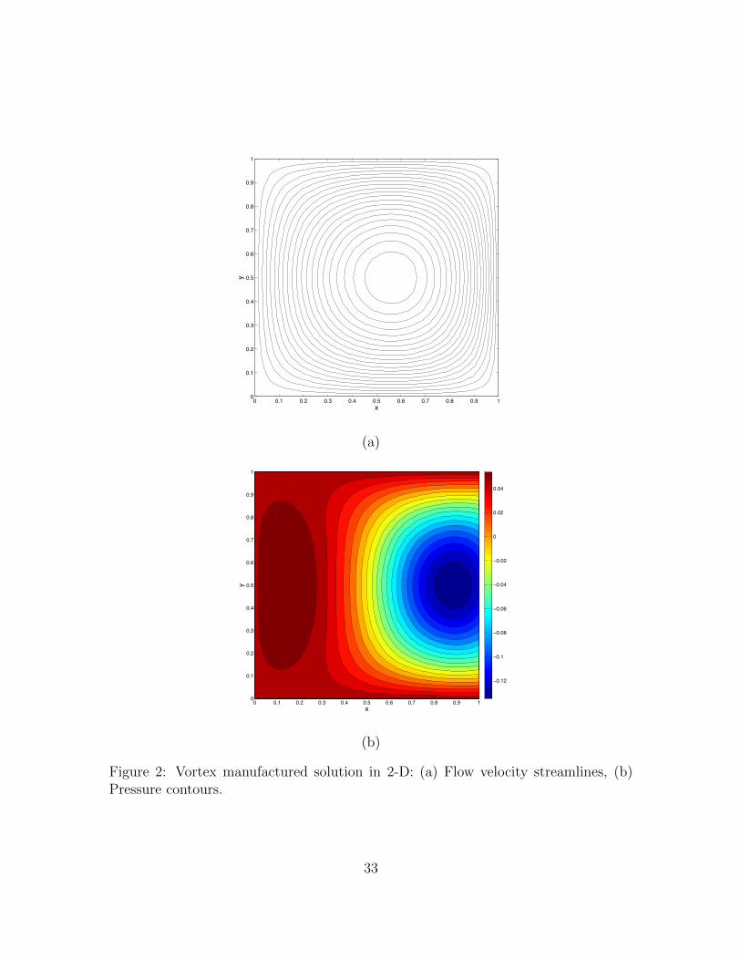
prescribed forcing is then clearly (u, p) = (u, p), and this solution is unique provideda smallness condition is satisfied. The streamlines and pressure contours associatedwith the solution are plotted in Figure 2.

To confirm our theoretically derived error estimates, we have computed conver-gence rates for divergence-conforming B-spline discretizations of varying mesh size and

32

x

y

0 0.1 0.2 0.3 0.4 0.5 0.6 0.7 0.8 0.9 10

0.1

0.2

0.3

0.4

0.5

0.6

0.7

0.8

0.9

1

(a)

x

y

0 0.1 0.2 0.3 0.4 0.5 0.6 0.7 0.8 0.9 10

0.1

0.2

0.3

0.4

0.5

0.6

0.7

0.8

0.9

1

−0.12

−0.1

−0.08

−0.06

−0.04

−0.02

0

0.02

0.04

(b)

Figure 2: Vortex manufactured solution in 2-D: (a) Flow velocity streamlines, (b)Pressure contours.

33

Table 1: Steady vortex flow convergence rates in 2-D: Re = 1

Polynomial degree k′ = 1

h 1/4 1/8 1/16 1/32 1/64‖u− uh‖h 5.48e-2 2.80e-2 1.40e-2 7.00e-3 3.50e-3

order - 0.97 1.00 1.00 1.00|u− uh|H1(Ω) 5.48e-2 2.80e-2 1.40e-2 7.00e-3 3.50e-3

order - 0.97 1.00 1.00 1.00‖u− uh‖L2(Ω) 2.77e-3 8.16e-4 2.28e-4 6.10e-5 1.58e-5

order - 1.76 1.84 1.90 1.95‖p− ph‖L2(Ω) 5.04e-3 1.38e-3 3.49e-4 8.72e-5 2.18e-5

order - 1.87 1.98 2.00 2.00


h 1/4 1/8 1/16 1/32 1/64‖u− uh‖h 9.71e-3 2.33e-3 5.68e-4 1.40e-4 3.48e-5




order - 3.40 3.26 3.30 3.23


h 1/4 1/8 1/16 1/32 1/64‖u− uh‖h 9.86e-4 1.28e-4 1.66e-5 2.13e-6 2.72e-7




order - 4.29 4.03 3.98 3.98

34

Table 2: Robustness of 2-D divergence-free B-spline discretizations for increasing Re

Polynomial degree k′ = 1, h = 1/16

Re 0 1 10 100 1000 10000‖u− uh‖h 1.40e-2 1.40e-2 1.40e-2 1.40e-2 1.40e-2 1.40e-2|u− uh|H1(Ω) 1.40e-2 1.40e-2 1.40e-2 1.40e-2 1.40e-2 1.40e-2‖u− uh‖L2(Ω) 2.28e-4 2.28e-4 2.28e-4 2.28e-4 2.28e-4 2.28e-4‖p− ph‖L2(Ω) 3.49e-4 3.49e-4 1.98e-4 1.96e-4 1.96e-4 1.96e-4





Table 3: Instability of conservative 2-D Taylor-Hood discretizations for increasing Re

Q2/Q1 velocity/pressure pair, h = 1/16

Re 0 1 10 100 1000 10000|u− uh|H1(Ω) 6.78e-4 6.78e-4 7.11e-4 2.26e-3 2.16e-2 2.16e-1‖u− uh‖L2(Ω) 6.54e-6 6.54e-6 6.79e-6 1.97e-5 1.86e-4 2.35e-3‖p− ph‖L2(Ω) 1.96e-4 1.96e-4 1.96e-4 1.96e-4 1.96e-4 1.96e-4

35

polynomial degree. Furthermore, we have computed rates for a variety of Reynoldsnumbers

Re =UL

ν

where U is a velocity scale parameter and L is a length scale parameter. We take U =1 and L = 1. In Table 1, we have plotted our numerically computed convergence ratesfor Re = 1. First, note that our theoretically derived error estimates are confirmed.Second, note that the L2-norm of the pressure error optimally converges like O(hk

′+1),which is an improvement over our theoretically derived estimate. Third, note thatthe results in Table 1 are identical to the Stokes results appearing in Table 2 of [19].Hence, the introduction of convection has not affected our numerical error.

While our theoretically derived error estimates only cover flows with “small”Reynolds number (and indeed uniqueness is only guaranteed under a smallness condi-tion), we have investigated the effectiveness of our discretization for larger Reynoldsnumber flows and the two-dimensional forcing prescribed above. To compute theseflow solutions, we used a Newton-Raphson nonlinear solver in conjunction with con-tinuation. The results of this investigation are included in Table 2 for meshes with16 × 16 elements. Note that the velocity numerical errors in the tables appear in-dependent of the Reynolds number. Moreover, the pressure numerical errors seemto improve with increasing Reynolds number. Hence, we are able to recover the de-sired flow solution (u, p) for large Reynolds numbers. This observation attests to theenhanced stability properties of our discretization for nonlinear flow problems evenin the absence of any external stabilization mechanisms. To contrast our methodol-ogy with standard mixed finite element discretizations, we have repeated the abovecomputations for conservative Taylor-Hood [24] finite element approximations, us-ing again a continuation method in conjunction with a Newton-Raphson nonlinearsolver. The results of these computations are included in Table 3. Note that while thepressure error is well-behaved, the velocity error diverges with increasing Reynoldsnumber. We believe that this divergence is inherently tied to the fact the Taylor-Hoodapproximations only satisfy the divergence-free constraint approximately.

8.2 Three-dimensional Manufactured Solution

As a second numerical experiment, we consider a three-dimensional manufacturedsolution representing a single vortical filament. Let

Ω ≡ (0, 1)3

andf ≡ ∇ · (u⊗ u)−∇ · (2ν∇su) +∇p

withu = curlφ,

36

Figure 3: Vortex manufactured solution in 3-D: Flow velocity streamlines colored byvelocity magnitude.

φ =

x(x− 1)y2(y − 1)2z2(z − 1)2

0x2(x− 1)2y2(y − 1)2z(z − 1)

,and

p = sin(πx) sin(πy)− 4

π2.

Again, homogeneous boundary conditions are applied along the boundary ∂Ω, andthe pressure is enforced to satisfy

∫Ωpdx = 0. A solution to the steady Navier-Stokes

equations with the prescribed forcing is then clearly (u, p) = (u, p), and for sufficientlysmall data, this solution is unique. Streamlines associated with the exact solution areplotted in Figure 3.

For Re = 1 flow (with Re = 1/ν), we have computed convergence rates fordivergence-conforming B-spline discretizations of varying mesh size and polynomialdegree. In Table 4, we have listed our numerically computed convergence rates.First, note that our theoretically derived error estimates are confirmed. Second, notethat the L2-norm of the pressure error optimally converges like O(hk

′+1), which isan improvement over our theoretically derived estimate. Third, note that, as in thetwo-dimensional setting, the results in Table 4 are identical to the Stokes resultsappearing in Table 5 of [19]. Hence, the introduction of convection has not affectedour numerical error.

Again, while our theoretically derived error estimates only cover flows with “small”Reynolds number, we have investigated the effectiveness of our discretization for larger

37

Table 4: Steady vortex flow convergence rates in 3-D: Re = 1.


h 1/2 1/4 1/8 1/16 1/32‖u− uh‖h 1.83e-2 8.98e-3 4.18e-3 1.99e-3 9.62e-4


order - 0.98 1.02 1.01 1.00‖u− uh‖L2(Ω) 1.35e-3 3.68-4 1.03e-4 2.81e-5 7.40e-6


order - 1.87 2.05 2.02 1.97


h 1/2 1/4 1/8 1/16 1/32‖u− uh‖h 6.50e-3 1.54e-3 4.10e-4 9.51e-5 2.15e-5




order - 3.24 2.99 2.97 2.97

Table 5: Robustness of 3-D divergence-free B-spline discretizations for increasing Re





38

Reynolds number flows and the three-dimensional forcing prescribed above. We useda Newton-Raphson nonlinear solver in conjunction with continuation. The resultsof this investigation are included in Table 5 for meshes with 16 × 16 × 16 elements.Note that the velocity and pressure numerical errors appearing in the tables areindependent of the Reynolds number. Hence, we are able to recover the desired flowsolution (u, p) for large Reynolds numbers.

8.3 Kovasznay Flow

As a third numerical experiment, we consider Kovasznay flow. Kovasznay flow refersto the flow behind an infinite two-dimensional grid, and it is often utilized as aconvergence test for Navier-Stokes discretizations. The flow pattern is periodic andcan be analytically derived [27]. Indeed, denoting Re = 1

ν, the flow solution satisfies

u =

[1− eλx cos(2πy)λ2πeλx cos(2πy).

]and

p = 1−e2λx2

.

where

λ =Re

2−√

Re2

4+ 4π2.

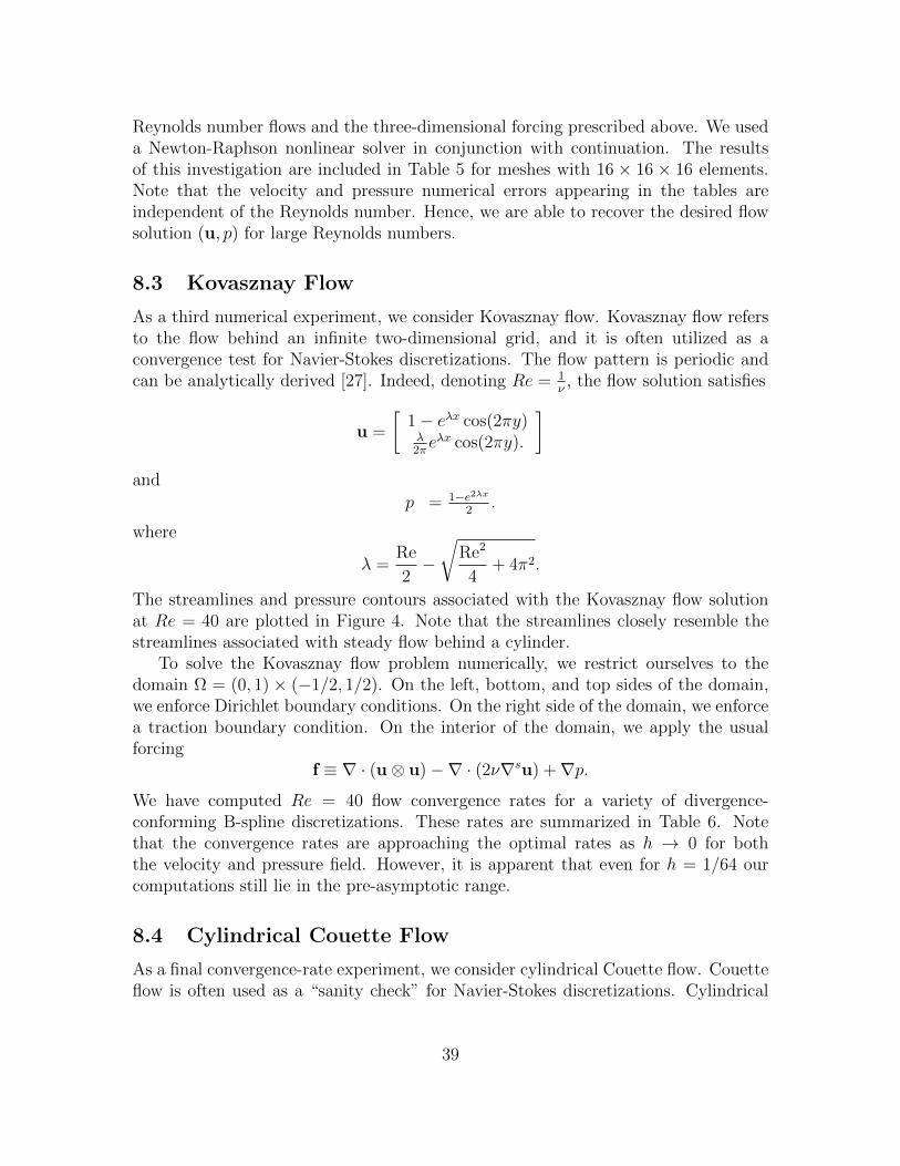
The streamlines and pressure contours associated with the Kovasznay flow solutionat Re = 40 are plotted in Figure 4. Note that the streamlines closely resemble thestreamlines associated with steady flow behind a cylinder.

To solve the Kovasznay flow problem numerically, we restrict ourselves to thedomain Ω = (0, 1) × (−1/2, 1/2). On the left, bottom, and top sides of the domain,we enforce Dirichlet boundary conditions. On the right side of the domain, we enforcea traction boundary condition. On the interior of the domain, we apply the usualforcing

f ≡ ∇ · (u⊗ u)−∇ · (2ν∇su) +∇p.

We have computed Re = 40 flow convergence rates for a variety of divergence-conforming B-spline discretizations. These rates are summarized in Table 6. Notethat the convergence rates are approaching the optimal rates as h → 0 for boththe velocity and pressure field. However, it is apparent that even for h = 1/64 ourcomputations still lie in the pre-asymptotic range.

8.4 Cylindrical Couette Flow

As a final convergence-rate experiment, we consider cylindrical Couette flow. Couetteflow is often used as a “sanity check” for Navier-Stokes discretizations. Cylindrical

39

x

y

0 0.1 0.2 0.3 0.4 0.5 0.6 0.7 0.8 0.9 1−0.5

−0.4

−0.3

−0.2

−0.1

0

0.1

0.2

0.3

0.4

0.5

(a)

x

y

0 0.1 0.2 0.3 0.4 0.5 0.6 0.7 0.8 0.9 1−0.5

−0.4

−0.3

−0.2

−0.1

0

0.1

0.2

0.3

0.4

0.5

0

0.05

0.1

0.15

0.2

0.25

0.3

0.35

0.4

(b)

Figure 4: Steady Kovasznay flow: (a) Streamlines for Re = 40, (b) Pressure contoursfor Re = 40.

40

Table 6: Steady Kovasznay flow convergence rates: Re = 40


h 1/4 1/8 1/16 1/32 1/64|u− uh|H1(Ω) 1.39e0 7.31e-1 3.69e-1 1.84e-1 9.19e-2



order - 1.42 1.65 1.81 1.85


h 1/4 1/8 1/16 1/32 1/64|u− uh|H1(Ω) 4.59e-1 1.17e-1 2.78e-2 6.69e-3 1.64e-3



order - 2.22 2.79 2.87 2.88


h 1/4 1/8 1/16 1/32 1/64|u− uh|H1(Ω) 1.29e-1 1.52e-2 1.94e-3 2.55e-4 3.31e-5



order - 3.11 3.49 3.45 3.72

41

Couette flow is a more realistic problem which describes the flow between two concen-tric rotating cylinders. Here, we consider flow between a fixed outer cylinder and arotating inner cylinder. The problem setup is illustrated in Figure 5(a). No externalforcing is applied. The velocity field for this flow assumes the form

u =

[uθ(r) sin(θ)uθ(r) cos(θ)

]where

uθ(r) = Ar +B

r,

(r, θ) are polar coordinates with respect to the center of the cylinders, and

A = −Ωinδ2

1− δ2, B = Ωin

r2in

(1− δ2), Ωin =

U

rin, δ =

rinrout

.

We have depicted this velocity field in Figure 5(b). The pressure field for cylindricalCouette flow is axisymmetric and satisfies the differential equation

∂p(r)

∂r=uθ(r)

2

r. (101)

The above differential equation coupled with the constraint∫Ω

pdx = 0

determines the pressure field uniquely. In what follows, we assume rin = 1, rout = 2,and U = 1.

We have computed convergence rates for a variety of divergence-conforming B-spline discretizations and for Re = 40. To represent the annular domain in ourcomputations, we employed the polar mapping

F(ξ1, ξ2) =

[((rout − rin)ξ2 + rin) sin(2πξ1)((rout − rin)ξ2 + rin) cos(2πξ1)

],∀(ξ1, ξ2) ∈ (0, 1)2 (102)

and periodic B-splines of maximal continuity in the ξ1-direction (see Section 2 of [17]).It should be emphasized that we do not use the polar form of the steady Navier-Stokesequations. Rather, we utilize the polar mapping to define our divergence-conformingB-splines in physical space and then employ the Cartesian-based variational formu-lation discussed in this chapter. The results of our computations are summarizedin Table 7. Note from the table that all of our theoretically derived error estimatesare confirmed. Furthermore, we have obtained axisymmetric velocity fields with zeroradial components, and the discrete pressure field converges at optimal order. Wehave additionally simulated the cylindrical Couette flow problem using a multi-patchNURBS construction (see Subsection 8.4 of [19]) and obtained identical discrete ve-locity fields and slightly differing (yet still optimally convergent) discrete pressurefields.

42

Dout

Din

U

(a)

2 1.5 1 0.5 0 0.5 1 1.5 22

1.5

1

0.5

0

0.5

1

1.5

2

x

y

(b)

Figure 5: Cylindrical Couette flow: (a) Problem setup, (b) Flow velocity arrows.

43

h/h0 = 1/2

h/h0 = 1/4

h/h0 = 1/8

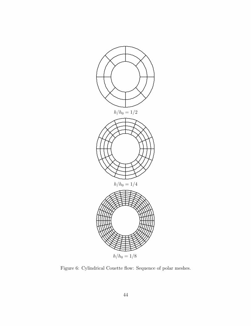
Figure 6: Cylindrical Couette flow: Sequence of polar meshes.

44

Table 7: Cylindrical Couette flow convergence rates: Re = 40


h/h0 1/2 1/4 1/8 1/16 1/32‖u− uh‖h 5.42e-1 2.63e-1 1.26e-1 6.12e-2 2.99e-2


order - 0.95 0.99 1.00 1.00‖u− uh‖L2(Ω) 5.00e-2 1.53-2 4.28e-3 1.14e-3 2.94e-4


order - 1.90 1.96 1.98 1.99‖ur − (ur)h‖L2(Ω) 0 0 0 0 0


h/h0 1/2 1/4 1/8 1/16 1/32‖u− uh‖h 9.77e-2 2.42e-2 5.64e-3 1.32e-3 3.14e-4




order - 2.82 2.86 2.90 2.94‖ur − (ur)h‖L2(Ω) 0 0 0 0 0


h/h0 1/2 1/4 1/8 1/16 1/32‖u− uh‖h 2.01e-2 2.67e-3 3.27e-4 4.01e-5 4.98e-6




order - 3.50 3.52 3.74 3.88‖ur − (ur)h‖L2(Ω) 0 0 0 0 0

45

H

H

U

Figure 7: Lid-driven flow in a two-dimensional cavity: Problem setup.

9 Benchmark Problems

In this section, we investigate the effectiveness of our methodology as applied totwo benchmark problems: two-dimensional lid-driven cavity flow and confined jetimpingement. As previously, we choose Nitsche’s penalty constant as Cpen = 5(k′+1)for all of the following examples, and we employ uniform parametric meshes, linearparametric mappings, and B-spline spaces of maximal continuity.

9.1 Two-dimensional Lid-driven Cavity Flow

Two-dimensional lid-driven cavity flow is widely considered to be one of the classicaltest problems for the validation of numerical discretizations for incompressible flowsimulation. In the presence of increasing Reynolds number, lid-driven cavity flowloses its symmetry and eventually becomes unsteady. The problem setup for lid-driven cavity flow is shown in Figure 7. For the computations here, H and U aredefined to be 1. The Reynolds number associated with the flow is defined to be

Re =UH

ν.

The left, right, and bottom sides of the cavity are fixed no-slip walls while the topside of the cavity is a wall which slides to the right with velocity magnitude U . The

46

x

y

0 0.1 0.2 0.3 0.4 0.5 0.6 0.7 0.8 0.9 10

0.1

0.2

0.3

0.4

0.5

0.6

0.7

0.8

0.9

1

Figure 8: Lid-driven cavity flow: Streamlines for Re = 100.

forcing f is defined to be zero. The pressure and stress fields associated with this flowexperience corner singularities which impede the convergence of numerical methodsand expose unstable velocity/pressure pairs. Furthermore, the velocity boundarycondition is discontinuous at the upper left and right corners of the domain. Inclassical finite element analysis, this boundary condition must be replaced with anapproximate “smooth” boundary condition. Here, as the prescribed slip boundarycondition is weakly enforced, we do not have to invoke such an approximation andcan instead directly utilize the discontinuous boundary condition.

We have numerically simulated lid-driven cavity flow at Re = 100, Re = 400, andRe = 1000 using a variety of divergence-conforming B-spline discretizations. Stream-lines computed using a mesh of degree k′ = 1 and size h = 1/128 are plotted in Figures8, 9, and 10 for Re = 100, Re = 400, and Re = 1000, respectively. These computedstreamlines are visually indistinguishable from benchmark streamlines appearing inthe literature.

We have compared our numerical results with the classical benchmark results ofGhia et al. [21] for three different polynomial degrees (k′ = 1, k′ = 2, k′ = 3),three different mesh sizes (h = 1/32, h = 1/64, and h = 1/128), and the selectedReynolds numbers. The results of Ghia were obtained using a second-order upwindfinite difference method on a stretched mesh with 1292 grid points. In Figures 11(a),12(a), and 13(a), we have compared our k′ = 1, Re = 100 values for the horizontal

47

x

y

0 0.1 0.2 0.3 0.4 0.5 0.6 0.7 0.8 0.9 10

0.1

0.2

0.3

0.4

0.5

0.6

0.7

0.8

0.9

1


component of the velocity field along the vertical center line with those of Ghia,and in Figures 11(b), 12(b), and 13(b), we have compared our k′ = 1, Re = 100values for the vertical component of the velocity field along the horizontal centerline. Note that our centerline velocity results are roughly independent of the meshsize. Second, note that while our results ostensibly match those of Ghia, there arediscernible quantitative differences between the two sets of results even for our finestmesh. To investigate these differences further, we have employed a set of convergedpseudospectral results that were obtained via a subtraction method to remove theleading terms of the corner singularities [5]. In Table 8, we have compared ourcenterline results with these converged results as well as the results of Ghia. Notethat our results are much more accurate than the results of Ghia for all mesh sizesand polynomial degrees. Furthermore, our results for k′ = 2 and k′ = 3 on a 64× 64element mesh are indistinguishable from the converged pseudospectral results. Thisattests to the effectiveness of our discretization with increasing k′, even in the presenceof singularities. We should also again remark that these results were obtained withoutstretched meshes and without stabilization. We believe that the combination of exactmass conservation and weak enforcement of the no-slip condition plays a pivotal rolein the enhanced accuracy of our discretization scheme.

In Figures 14(a), 15(a), and 16(a), we have compared our k′ = 1, Re = 400 valuesfor the horizontal component of the velocity field along the vertical center line with

48

x

y

0 0.1 0.2 0.3 0.4 0.5 0.6 0.7 0.8 0.9 10

0.1

0.2

0.3

0.4

0.5

0.6

0.7

0.8

0.9

1


those of Ghia, and in Figures 14(b), 15(b), and 16(b), we have compared our k′ = 1,Re = 400 values for the vertical component of the velocity field along the horizontalcenter line. Note that our Re = 400 results match the results of Ghia better thanthe Re = 100 results. In fact, our Re = 400 results are nearly indistinguishable fromthe benchmark results on the finest mesh. This is encouraging as the Ghia Re = 400results match well with highly-accurate extrapolated results in the literature [34].Moreover, our results for the coarsest mesh match the results of Ghia better than anycomparable second-order results we have seen in the literature. In Table 8, we havecompared our centerline results with the results of Ghia along with our results fork′ = 2 and k′ = 3 on a 64×64 element mesh. Note that our results appear to convergequickly with increasing k′, despite the increased smoothness of our discrete spaces.By using our k′ = 3 results as a benchmark, we see our k′ = 1 results are considerablymore accurate than Ghia’s results for h ≤ 1/64. Unfortunately, no pseudospectralresults are available to use as comparison.

In Figures 17(a), 18(a), and 19(a), we have compared our k′ = 1, Re = 1000 valuesfor the horizontal component of the velocity field along the vertical center line withthose of Ghia, and in Figures 17(b), 18(b), and 19(b), we have compared our k′ = 1,Re = 1000 values for the vertical component of the velocity field along the horizontalcenter line. This is a more challenging test case than either the Re = 100 or Re = 400flows, and the coarse 32 × 32 element mesh is not nearly fine enough to resolve theflow features. Nonetheless, our results for this coarse mesh better match the results

49

Table 8: Two-dimensional lid-driven cavity flow: Extrema of the velocity through thecenterlines of the cavity.

Re = 100

Method umin vmax vminB-spline, k′ = 1 and h = 1/32 −0.21551 0.18054 −0.25472B-spline, k′ = 1 and h = 1/64 −0.21443 0.17991 −0.25409B-spline, k′ = 1 and h = 1/128 −0.21414 0.17966 −0.25387B-spline, k′ = 2 and h = 1/64 −0.21404 0.17957 −0.25379B-spline, k′ = 3 and h = 1/64 −0.21404 0.17957 −0.25380

Pseudospectral (Ref. [5]) −0.21404 0.17957 −0.25380Ghia et al. (Ref. [21]) −0.21090 0.17527 −0.24533

Re = 400


Ghia et al. (Ref. [21]) −0.32376 0.30203 −0.44993

Re = 1000


Pseudospectral (Ref. [5]) −0.38857 0.37694 −0.52707Ghia et al. (Ref. [21]) −0.38289 0.37095 −0.51550

50

0.5 0 0.5 10

0.2

0.4

0.6

0.8

1

u/U

y/H

h = 1/32Ghia et. al

(a)

0 0.2 0.4 0.6 0.8 10.3

0.2

0.1

0

0.1

0.2

x/H

v/U

h = 1/32Ghia et. al

(b)

Figure 11: Lid-driven cavity flow: Velocity field for k′ = 1, h = 1/32, and Re = 100.(a) Value of the horizontal component of the velocity field along the vertical centerline, (b) Value of the vertical component of the velocity field along the horizontalcenter line.

51

0.5 0 0.5 10

0.2

0.4

0.6

0.8

1

u/U

y/H

h = 1/64Ghia et. al

(a)

0 0.2 0.4 0.6 0.8 10.3

0.2

0.1

0

0.1

0.2

x/H

v/U

h = 1/64Ghia et. al

(b)


52

0.5 0 0.5 10

0.2

0.4

0.6

0.8

1

u/U

y/H

h = 1/128Ghia et. al

(a)

0 0.2 0.4 0.6 0.8 10.3

0.2

0.1

0

0.1

0.2

x/H

v/U


(b)


53

0.5 0 0.5 10

0.2

0.4

0.6

0.8

1

u/U

y/H

h = 1/32Ghia et. al

(a)

0 0.2 0.4 0.6 0.8 10.6

0.4

0.2

0

0.2

0.4

x/H

v/U

h = 1/32Ghia et. al

(b)


54

0.5 0 0.5 10

0.2

0.4

0.6

0.8

1

u/U

y/H

h = 1/64Ghia et. al

(a)

0 0.2 0.4 0.6 0.8 10.6

0.4

0.2

0

0.2

0.4

x/H

v/U

h = 1/64Ghia et. al

(b)


55

0.5 0 0.5 10

0.2

0.4

0.6

0.8

1

u/U

y/H


(a)

0 0.2 0.4 0.6 0.8 10.6

0.4

0.2

0

0.2

0.4

x/H

v/U


(b)


56

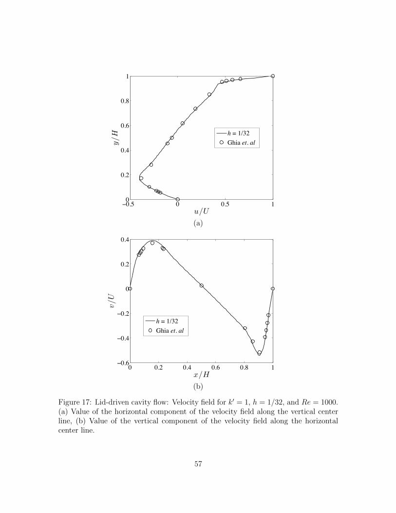
0.5 0 0.5 10

0.2

0.4

0.6

0.8

1

u/U

y/H

h = 1/32Ghia et. al

(a)

0 0.2 0.4 0.6 0.8 10.6

0.4

0.2

0

0.2

0.4

x/H

v/U

h = 1/32Ghia et. al

(b)


57

0.5 0 0.5 10

0.2

0.4

0.6

0.8

1

u/U

y/H

h = 1/64Ghia et. al

(a)

0 0.2 0.4 0.6 0.8 10.6

0.4

0.2

0

0.2

0.4

x/H

v/U

h = 1/64Ghia et. al

(b)


58

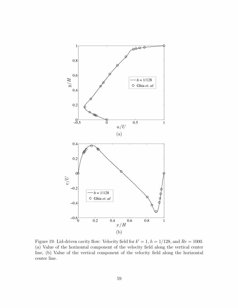
0.5 0 0.5 10

0.2

0.4

0.6

0.8

1

u/U

y/H


(a)

0 0.2 0.4 0.6 0.8 10.6

0.4

0.2

0

0.2

0.4

x/H

v/U


(b)


59

of Ghia than any comparable second-order results we have seen in the literature. Ourresults for the 64×64 and 128×128 element meshes match Ghia’s results even better.In Table 8, we have compared our centerline results with the results of Ghia alongwith a set of converged pseudospectral results with singularity subtraction [5]. Asexpected, the results of Ghia are more accurate than our coarse mesh results, but ourresults for the 64× 64 element mesh are comparable in accuracy and our results forthe 128×128 element mesh are considerably more accurate. We also computed resultsfor the 64× 64 element mesh for polynomial degrees k′ = 2 and k′ = 3 and found ourresults quickly improved with increasing polynomial degree. Indeed, our results fork′ = 3 are nearly indistinguishable from the converged pseudospectral results.

To compute all of these flow examples, we utilized the Newton-Raphson methodin conjunction with continuation. Specifically, for the Re = 100 simulations, weemployed Newton-Raphson using the results of a corresponding Stokes simulation asan initial guess. For the Re = 400 simulations, we employed Newton-Raphson usingthe results of the Re = 100 simulations as an initial guess, and so on. We founda maximum of four Newton-Raphson steps were required to achieve a sufficientlyaccurate solution for each nonlinear solve. Using this procedure, we have been ableto successfully simulate flows upwards of Re = 3200 on relatively coarse meshes. Wehave also been able to reproduce all of the results presented here by a more expensivedynamic approach in which the solution is evolved from an initial condition by theunsteady Navier-Stokes equations.

9.2 Confined Jet Impingement

Impinging jets are commonly used in engineering applications due to their enhancedheat and mass transfer characteristics. Impinging jets even occur in blood vessels andare believed to play a role in atherogenesis [20]. Many discretization schemes yielda velocity field with spurious nonzero divergence when applied to the simulation ofincompressible jet impingement, even at small and moderate Reynolds numbers. Asour proposed discretization satisfies the divergence-free constraint exactly, it does notsuffer from this non-physical behavior.

The physical problem of confined jet impingement is illustrated in Figure 20. Fluidflows from one pipe into a second pipe lying perpendicular to the first. To simulatethis flow, we use a two-dimensional mathematical idealization which is illustrated inFigure 21. Along the left hand side of the domain, a symmetry condition is appliedas we only model half of the jet system. Along the bottom side of the domain, no-slip and no-penetration boundary conditions are enforced. Along the top side of thedomain, two different sets of boundary conditions are applied. Along the first D/2length of the top side, an inflow boundary condition is applied. Along the remainderof the top side, no-slip and no-penetration boundary conditions are enforced. Alongthe right hand side of the domain, a zero-traction boundary condition is enforced.The height of the domain is set as H, and the length of the domain, L, is chosen long

60

Stagnation Region

Flow Flow

Flow

Figure 20: Confined jet impingement: Physical setup.

L

H

U

D/2

Outflow

BC

No-slip Walls

Inflow

BC

Symmetry

BC

Figure 21: Confined jet impingement: Model problem description.

61

enough such that the flow exiting the pipe is parallel to the outflow plane. For thecomputations here, D = H = 1 and L = 8. The inflow speed is set to be U = 1. TheReynolds number for the flow is defined as Re = UH/ν.

We have simulatedRe = 50 confined jet impingement for two divergence-conformingB-spline discretizations of polynomial degree k′ = 1 corresponding to mesh lengths ofh = 1/16 and h = 1/32. The resulting velocity fields are plotted in Figures 22 and 23.First, note that the computed streamlines for the two meshes are indistinguishable.Second, note that the velocity fields are smooth and free from spurious oscillations.To compare our simulation results with those of a classical mixed method, we havesimulated the impingement problem for a conservative Taylor-Hood finite elementdiscretization with mesh length h = 1/8. This discretization contains approximatelythe same number of velocity degrees of freedom as the preceding coarse B-splinediscretization. The velocity field resulting from the Taylor-Hood discretization isplotted in Figure 24. Note that the contours of the velocity field roughly match thevelocity contours resulting from the divergence-conforming B-spline discretizations.However, the velocity field resulting from the Taylor-Hood discretization exhibits sig-nificant non-physical compressibility. We have conducted numerical investigations ofconfined jet impingement at other Reynolds numbers and obtained similar results tothose reported here.

10 Conclusions

In this paper, divergence-conforming B-spline discretizations have been presentedfor the steady Navier-Stokes equations utilizing a variational formulation written inconservation form. Tangential velocity boundary conditions are implemented weaklyusing Nitsche’s method. The formulation yields velocity fields that are pointwisedivergence-free on general mapped geometries. A collection of stability and errorestimates have been derived for flows subject to a smallness condition, and thesetheoretical results have been confirmed and supplemented by numerical simulationsof problems with known analytical solutions. In fact, these numerical simulationshave revealed that the proposed discretizations are robust with respect to Reynoldsnumber, a property not shared by classical finite elements such as the Taylor-Hoodelement. The new discretizations have also been applied to a selection of benchmarkproblems where the advantages of the new methodology over classical methods havebeen highlighted. In future work, we plan to extend the present developments to theunsteady Navier-Stokes equations and generalize to locally-refined meshes.

Acknowledgements

We thank Annalisa Buffa and Giancarlo Sangalli for their useful discussions regardingthis work. The authors were partially supported by the Office of Naval Research under

62

contract number N00014-08-0992. John A. Evans was additionally partially supportedby the Department of Energy Computational Science Graduate Fellowship, providedunder grant number DE-FG02-97ER25308. This support is gratefully acknowledged.

References

[1] D N Arnold. An interior penalty finite element method with discontinuous ele-ments. SIAM Journal on Numerical Analysis, 19:742–760, 1979.

[2] Y Bazilevs and T J R Hughes. Weak imposition of Dirichlet boundary conditionsin fluid mechanics. Computers and Fluids, 36:12–26, 2007.

[3] Y Bazilevs, C M Michler, V M Calo, and T J R Hughes. Weak Dirichlet bound-ary conditions for wall-bounded turbulent flows. Computer Methods in AppliedMechanics and Engineering, 196:4853–4862, 2007.

[4] Y Bazilevs, C M Michler, V M Calo, and T J R Hughes. Isogeometric varia-tional multiscale modeling of wall-bounded turbulent flows with weakly-enforcedboundary conditions on unstretched meshes. Computer Methods in Applied Me-chanics and Engineering, 199:780–790, 2010.

[5] O Botella and R Peyret. Benchmark spectral results on the lid-driven cavityflow. Computers and Fluids, 27:421–433, 1998.

[6] S C Brenner. Korn’s inequalities for piecewise H1 vector fields. Mathematics ofComputation, 73:1067–1087, 2003.

[7] A.N. Brooks and T.J.R. Hughes. Streamline upwind/Petrov-Galerkin formula-tions for convection dominated flows with particular emphasis on the incom-pressible Navier-Stokes equations. Computer Methods in Applied Mechanics andEngineering, 32:199–259, 1982.

[8] A Buffa, C de Falco, and R Vazquez. Isogeometric analysis: Stable elements forthe 2D Stokes equation. International Journal for Numerical Methods in Fluids,65:1407–1422,20–30, 2011.

[9] A Buffa, J Rivas, G Sangalli, and R Vazquez. Isogeometric discrete differentialforms in three dimensions. SIAM Journal on Numerical Analysis, 49:818–844,2011.

[10] A Buffa, G Sangalli, and R Vazquez. Isogeometric analysis in electromagnetics:B-splines approximation. Computer Methods in Applied Mechanics and Engi-neering, 199:1143–1152, 2010.

63

[11] B Cockburn, G Kanschat, and D Schotzau. A locally conservative LDG methodfor the incompressible Navier-Stokes equations. Mathematics of Computation,74:1067–1095, 2004.

[12] B Cockburn, G Kanschat, and D Schotzau. A note on discontinuous Galerkindivergence-free solutions of the Navier-Stokes equations. SIAM Journal on Sci-entific Computing, 31:61–73, 2007.

[13] J A Cottrell, T J R Hughes, and Y Bazilevs. Isogeometric Analysis: TowardIntegration of CAD and FEA. Wiley, 2009.

[14] C R de Boor. A Practical Guide to Splines. Springer-Verlag, 1978.

[15] J Douglas and T Dupont. Interior Penalty Procedures for Elliptic and ParabolicGalerkin Methods. Lecture Notes in Physics, 58, 1976.

[16] J A Evans. Divergence-free B-spline Discretizations for Viscous IncompressibleFlows. PhD thesis, The University of Texas at Austin, 2011.

[17] J A Evans, Y Bazilevs, I Babuska, and T J R Hughes. n-widths, sup-infs, andoptimality ratios for the k-version of the isogeometric finite element method.Computer Methods in Applied Mechanics and Engineering, 198:1726–1741, 2009.

[18] J A Evans and T J R Hughes. Explicit trace inequalities for isogeometric analysisand parametric finite elements. Technical report, ICES Report 11-17, 2011.

[19] J A Evans and T J R Hughes. Isogeometric divergence-conforming B-splinesfor the Darcy-Stokes-Brinkman equations. Technical report, ICES Report 12-03,2012.

[20] D L Fry. Atherogenesis: Initiating factors. CIBA Foundation Symposium, 12:93–125, 1973.

[21] U Ghia, K N Ghia, and C T Shin. High-Re solutions for incompressible flow usingthe Navier-Stokes equations and a multigrid method. Journal of ComputationalPhysics, 48:387–411, 1982.

[22] V Girault and P A Raviart. Finite Element Methods for Navier-Stokes Equations.Theory and Algorithms. Springer-Verlag, 1986.

[23] K Hollig. Finite Element Methods with B-splines. Society for Industrial andApplied Mathematics, 2003.

[24] P Hood and C Taylor. Navier-Stokes equations using mixed interpolation. In J TOden, R H Gallagher, O C Zienkiewicz, and C Taylor, editors, Finite ElementMethods in Flow Problems, pages 121–132. University of Alabama in HuntsvillePress, 1974.

64

[25] T J R Hughes, L P Franca, and M Balestra. A new finite element formulation forcomputational fluid dynamics: V. Circumventing the Babuska-Brezzi condition:A stable Petrov-Galerkin formulation of the Stokes problem accomodating equal-order interpolations. Computer Methods in Applied Mechanics and Engineering,59:85–99, 1986.

[26] T J R Hughes and G N Wells. Conservation properties for the Galerkin and sta-bilised forms of the advection-diffusion and incompressible Navier-Stokes equa-tions. Computer Methods in Applied Mechanics and Engineering, 194:1141–1159,2005.

[27] L I G Kovasznay. Laminar flow behind a two-dimensional grid. MathematicalProceedings of the Cambridge Philosophical Society, 44:58–62, 1948.

[28] R J Labeur and G N Wells. Energy stable and momentum conserving hybridfinite element method for the incompressible Navier-Stokes equations. SIAMJournal on Scientific Computing. To appear.

[29] N C Nguyen, J Peraire, and B Cockburn. An implicit high-order hybridizablediscontinuous Galerkin method for the incompressible Navier-Stokes equations.Journal of Computational Physics, 230:1147–1170, 2011.

[30] J A Nitsche. Uber ein Variationspringzip zur Losung von Dirichlet-Problemembei Verwendung von Teilraumen, die keinen Randbedingungen unterworfen sind.Abhandlungen aus dem Mathematischen Seminar der Universit at Hamburg,36:9–15, 1971.

[31] S B Pope. Turbulent Flows. Cambridge University Press, 2003.

[32] P A Raviart and J M Thomas. A mixed finite element method for second orderelliptic problems. Lecture Notes in Mathematics, 606:292–315, 1977.

[33] H-G Roos, M Stynes, and L Tobiska. Numerical Methods for Singularly PerturbedDifferential Equations. Convection-Diffusion and Flow Problems. Springer, 1996.

[34] R Schreiber and H B Keller. Driven cavity flows by efficient numerical techniques.Journal of Computational Physics, 49:310–333, 1983.

[35] L L Schumaker. Spline functions: Basic theory. Cambridge Mathematical Li-brary, Cambridge University Press, 2007.

[36] D B Spalding. A single formula for the law of the wall. Journal of AppliedMechanics, 28:444–458, 1961.

65

[37] T E Tezduyar, M Behr, S Mittal, and J Liou. A new strategy for finite ele-ment computations involving moving boundaries and interfaces - The deforming-spatial-domain/space-time procedure: II. Computation of free-surface flows, two-liquid flows, and flows with drifting cylinders. Computer Methods in AppliedMechanics and Engineering, 94:353–371, 1992.

[38] H Triebel. Interpolation Theory, Function Spaces, Differential Operators, SecondEdition. Johann Ambrosius Barth, 1995.

[39] M F Wheeler. An elliptic collocation-finite element method with interior penal-ties. SIAM Journal on Numerical Analysis, 15:152–161, 1978.

[40] T A Zang. On the rotation and skew-symmetric forms for incompressible flowsimulations. Applied Numerical Mathematics, 7:27–40, 1991.

[41] S Zhang. A new family of stable mixed finite elements for 3D Stokes equations.Mathematics of Computation, 250:543–554, 2005.

66

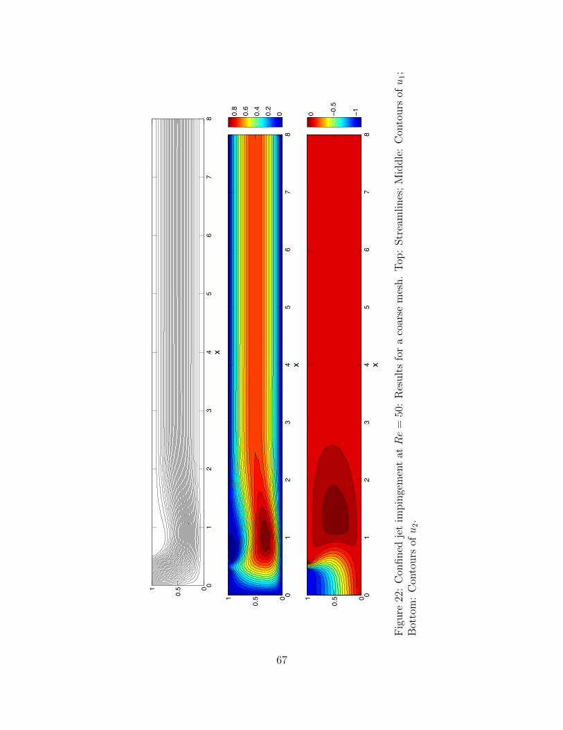
x

y

01

23

45

67

80

0.51

x

y

01

23

45

67

80

0.51

00.2

0.4

0.6

0.8

x

y

01

23

45

67

80

0.51

10.5

0

Fig

ure

22:

Con

fined

jet

impin

gem

ent

atRe

=50

:R

esult

sfo

ra

coar

sem

esh.

Top

:Str

eam

lines

;M

iddle

:C

onto

urs

ofu

1;

Bot

tom

:C

onto

urs

ofu

2.

67

x

y

01

23

45

67

80

0.51

x

y

01

23

45

67

80

0.51

00.2

0.4

0.6

0.8

x

y

01

23

45

67

80

0.51

10.5

0

Fig

ure

23:

Con

fined

jet

impin

gem

ent

atRe

=50

:R

esult

sfo

ra

reso

lved

mes

h.

Top

:Str

eam

lines

;M

iddle

:C

onto

urs

ofu

1;

Bot

tom

:C

onto

urs

ofu

2.

68

x

y

01

23

45

67

80

0.51

00.2

0.4

0.6

0.8

x

y

01

23

45

67

80

0.51

10.5

0

x

y

01

23

45

67

80

0.51

10.5

0

Fig

ure

24:

Con

fined

jet

impin

gem

ent

atRe

=50

:R

esult

sfo

rQ

2/Q

1ve

loci

ty/p

ress

ure

pai

r,h

=1/

8.T

op:

Con

tours

ofu

1;

Mid

dle

:C

onto

urs

ofu

2;

Bot

tom

:D

iver

gence

ofve

loci

tyfiel

d(i

nte

rpol

ated

atel

emen

tce

nte

rs).

69

ices report 12-15 isogeometric divergence-conforming b

Documents