i, term ect 2014 - university of alaska systemrfrith.uaa.alaska.edu/opsres/project.pdf · r, joan...

Des

amo

ur,

Jo

an

Star

lin

g, A

nn

e F

rith

, Ru

ssel

l

20

14

Op

era

tio

ns

Re

sea

rch

I, T

erm

G

rou

p P

roje

ct

Implement components of a linear programming model for an independent family-owned farming operation. Formulate a model based on crop yields, livestock productivity, and labor wages which in turn renders decisions on how to maximize total net worth. Obtain optimal monetary returns and run weather sensitivity analysis on income.

1 | P a g e

I. Components of the Linear Programming Model (Part a)

The decisions to made are how much acreage should be planted in each of the crops and how many cows and hens to have for the coming year. The constraints on these decisions are amount of labor hours available, the investment funds available, the number of acres available, the space available in the barn and chicken coop, and the minimum requirements for feed to be planted. The overall measure of performance is monetary worth, which is to be maximized.

II. Model Formulation (for a “good” year, Part b)

1. Plantings

a) Decision Variables

SA : Number of acres planted for soy beans;

CA : Number of acres planted for corn;

WA : Number of acres planted for wheat;

WSHrsReq : Winter and spring labor hours required for plantings;

SFHrsReq : Summer and fall labor hours required for plantings;

NVP : Net value of crops;

AP : Acres planted;

TC : Total number of cows;

TH : Total number of hens;

b) Formulae/Constraints

[AcresPlanted]AP = SA + CA + WA; [WSHrsPlanting]WSHrsReq = 1*SA + 0.9*CA + 0.6*WA; [SFHrsPlanting]SFHrsReq = 1.4*SA + 1.2*CA + 0.7*WA; [NetValPlanting]NVP = 70*SA + 60*CA + 40*WA; [CornAcres]CA >= TC; [WheatAcres]WA >= TH*0.05;

2. Livestock


HRM : Hours required per month;

Cows : Number of cows in inventory;

Hens : Number of hens in inventory;

GL : Grazing land required;

NACI : Net annual cash income;

BLV : Beginning livestock value;

2 | P a g e

ECLV : Ending current livestock value;

ENLV : Ending new livestock value;

NC : Number of new cows;

NH : Number of new hens;

IF : Investment fund;

TC : Total number of cows;

TH : Total number of hens;

LIF : Left over investment fund;

LE : Living expenses;

b) Formulae/Constraints

LE = $40,000

Cows = 30

Hens = 2000

TC = Cows + NC

TH = Hens NH

IF = $20000

HRM = 10*TC + 0.05*TH

GL = 2*TC + 0*TH

NACI = 850*(TC) + 4.25*(TH); BLV = 35000 + 5000; ECLV = 0.9*35000 + 0.75*5000; 1500*NC + 3*NH <= 20000; ENLV = (0.9*1500)*NC + (0.75*3)*NH; TC <= 42; TH <= 5000; EVL = ECLV + ENLV; LIF = IF - 1500*NC - 3*NH;

3. Neighboring Farm Work


WSHrs : Hours worked in winter and spring;

3 | P a g e

SFHrs : Hours worked in summer and fall;

b) Wage Formula

Wages = 5*WSHrs + 5.50*SFHrs

4. Model Formulae (LINGO)

a) [TotalMonetaryWorth]max = (NVP + NACI + Wages) + (EVL + LIF) – LE;

b) [TotalAcreage]AP + GL <= 640;

c)[WSHours]WSHrsReq + 6*HRM + WSHrs <= 4000;

d)[SFHours]SFHrsReq + 6*HRM + SFHrs <= 4500;

See appendix for LINGO implementation and results.

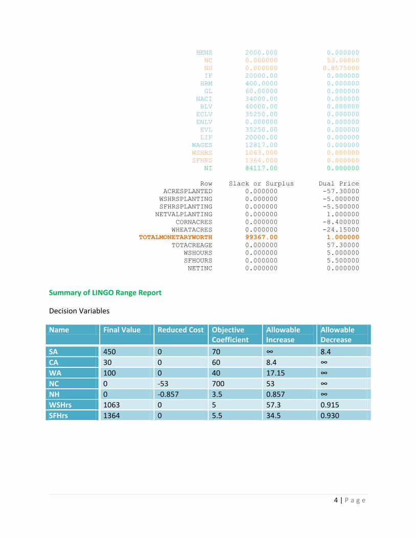
III. Optimal Solution, Model Sensitivity, and Objective Function Value (Parts c and d)

The model predicts that the family’s monetary worth at the end of the year will be $99,367.

LINGO Results

Global optimal solution found.

Objective value: 99367.00

Infeasibilities: 0.000000

Total solver iterations: 1

Elapsed runtime seconds: 0.03

Model Class: LP

Total variables: 21

Nonlinear variables: 0

Integer variables: 0

Total constraints: 23

Nonlinear constraints: 0

Total nonzeros: 64

Nonlinear nonzeros: 0

Variable Value Reduced Cost

AP 580.0000 0.000000

SA 450.0000 0.000000

CA 30.00000 0.000000

WA 100.0000 0.000000

WSHRSREQ 537.0000 0.000000

SFHRSREQ 736.0000 0.000000

NVP 37300.00 0.000000

TC 30.00000 0.000000

TH 2000.000 0.000000

LE 40000.00 0.000000

COWS 30.00000 0.000000

4 | P a g e

HENS 2000.000 0.000000

NC 0.000000 53.00000

NH 0.000000 0.8575000

IF 20000.00 0.000000

HRM 400.0000 0.000000

GL 60.00000 0.000000

NACI 34000.00 0.000000

BLV 40000.00 0.000000

ECLV 35250.00 0.000000

ENLV 0.000000 0.000000

EVL 35250.00 0.000000

LIF 20000.00 0.000000

WAGES 12817.00 0.000000

WSHRS 1063.000 0.000000

SFHRS 1364.000 0.000000

NI 84117.00 0.000000

Row Slack or Surplus Dual Price

ACRESPLANTED 0.000000 -57.30000

WSHRSPLANTING 0.000000 -5.000000

SFHRSPLANTING 0.000000 -5.500000

NETVALPLANTING 0.000000 1.000000

CORNACRES 0.000000 -8.400000

WHEATACRES 0.000000 -24.15000

TOTALMONETARYWORTH 99367.00 1.000000

TOTACREAGE 0.000000 57.30000

WSHOURS 0.000000 5.000000

SFHOURS 0.000000 5.500000

NETINC 0.000000 0.000000

Summary of LINGO Range Report

Decision Variables

Name Final Value Reduced Cost Objective Coefficient

Allowable Increase

Allowable Decrease

SA 450 0 70 ∞ 8.4

CA 30 0 60 8.4 ∞

WA 100 0 40 17.15 ∞

NC 0 -53 700 53 ∞

NH 0 -0.857 3.5 0.857 ∞

WSHrs 1063 0 5 57.3 0.915

SFHrs 1364 0 5.5 34.5 0.930

5 | P a g e

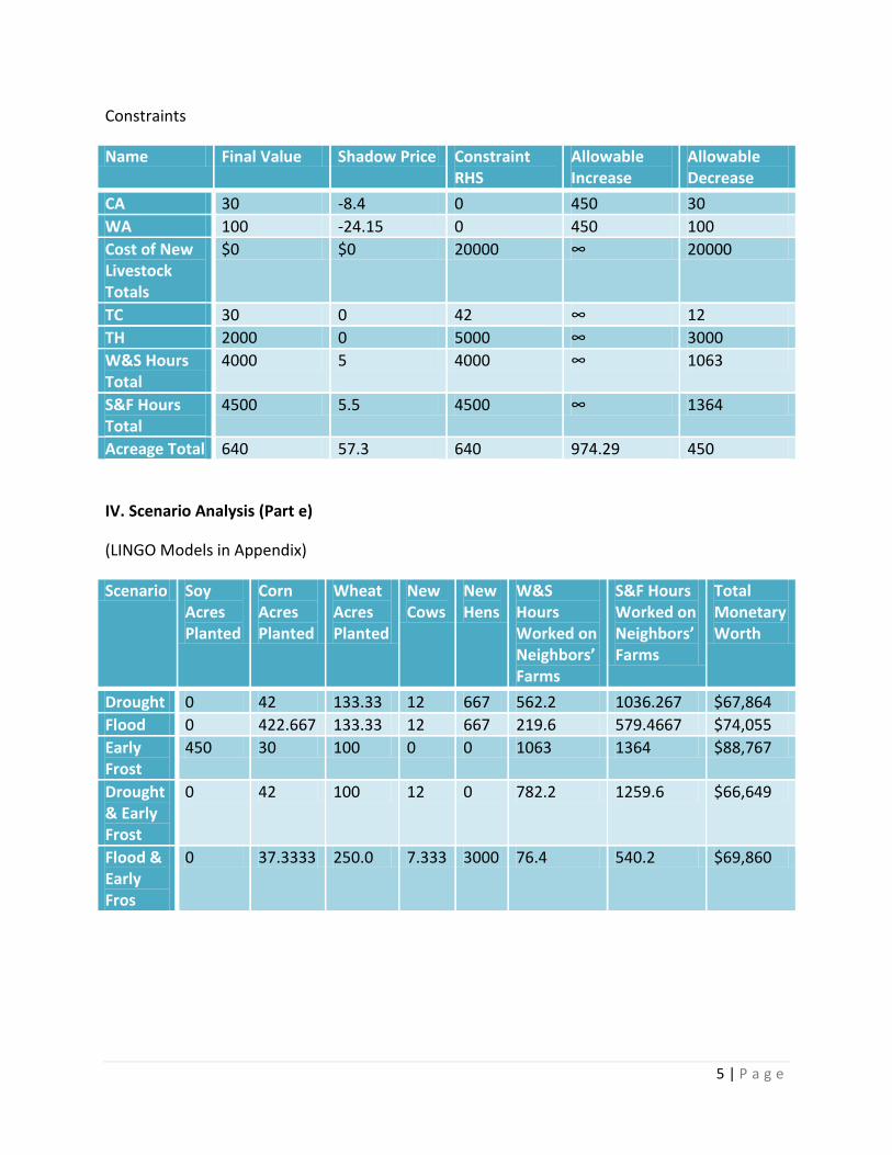
Constraints

Name Final Value Shadow Price Constraint RHS

Allowable Increase

Allowable Decrease

CA 30 -8.4 0 450 30

WA 100 -24.15 0 450 100

Cost of New Livestock Totals

$0 $0 20000 ∞ 20000

TC 30 0 42 ∞ 12

TH 2000 0 5000 ∞ 3000

W&S Hours Total

4000 5 4000 ∞ 1063

S&F Hours Total

4500 5.5 4500 ∞ 1364

Acreage Total 640 57.3 640 974.29 450

IV. Scenario Analysis (Part e)

(LINGO Models in Appendix)

Scenario Soy Acres Planted

Corn Acres Planted

Wheat Acres Planted

New Cows

New Hens

W&S Hours Worked on Neighbors’ Farms

S&F Hours Worked on Neighbors’ Farms

Total Monetary Worth

Drought 0 42 133.33 12 667 562.2 1036.267 $67,864

Flood 0 422.667 133.33 12 667 219.6 579.4667 $74,055

Early Frost

450 30 100 0 0 1063 1364 $88,767

Drought & Early Frost

0 42 100 12 0 782.2 1259.6 $66,649

Flood & Early Fros

0 37.3333 250.0 7.333 3000 76.4 540.2 $69,860

6 | P a g e

V. Additional Scenario Analysis (Climate conditions change during the year, Part f)

Family’s monetary worth at year’s end if the scenario is actually:

Optimal Solution Used

Good Weather

Drought Flood Early Frost Drought..EF Flood..EF

Good Weather

$99,367 $57,117 $70,417 $88,767 $53,717 $67,367

Drought $76,348 $67,864 $70,668 $74,174 $66,321 $69,581

Flood $94,962 $57,929 $74,055 $85,175 $54,482 $69,162

Early Frost $99,367 $57,117 $70,417 $88,767 $53,717 $67,367

Drought & Early Frost

$75,009 $67,859 $70,329 $73,169 $66,649 $69,409

Flood & Early Frost

$80,476 $67,676 $71,483 $77,230 $64,990 $69,860

The good weather solution is the riskiest. It has the widest swing from maximum to minimum

monetary worth. The flood solution appears to be the mid-range of the variability in the swing

from maximum to minimum monetary worth. The most conservative scenarios are drought,

drought/early frost, and flood/early frost.

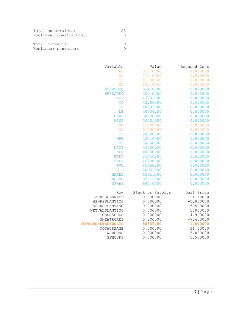
VI. Weighted Scenario Analysis (Parts g and h)

The expected net value for each of the crops is calculated as follows:

Soybeans: ($70)(0.4) + (-$10)(0.2) + ($15)(0.1) + ($50)(0.15) + (-$15)(0.1) + ($10)(0.05) = $34,

Corn: ($60)(0.4) + (-$15)(0.2) + ($20)(0.1) + ($40)(0.15) + (-$20)(0.1) + ($10)(0.05) = $27.5,

Wheat: ($40)(0.4) + ($0)(0.2) + ($10)(0.1) + ($30)(0.15) + (-$10)(0.1) + ($5)(0.05) = $20.75

See appendix for LINGO model.

The model predicts that the family’s monetary worth at the end of the year will be $80,537.

LINGO Results

Global optimal solution found.

Objective value: 80537.00

Infeasibilities: 0.000000

Total solver iterations: 1

Elapsed runtime seconds: 0.05

Model Class: LP

Total variables: 20

Nonlinear variables: 0

Integer variables: 0

7 | P a g e

Total constraints: 22

Nonlinear constraints: 0

Total nonzeros: 60

Nonlinear nonzeros: 0

Variable Value Reduced Cost

AP 556.0000 0.000000

SA 414.0000 0.000000

CA 42.00000 0.000000

WA 100.0000 0.000000

WSHRSREQ 511.8000 0.000000

SFHRSREQ 700.0000 0.000000

NVP 17306.00 0.000000

TC 42.00000 0.000000

TH 2000.000 0.000000

LE 40000.00 0.000000

COWS 30.00000 0.000000

HENS 2000.000 0.000000

NC 12.00000 0.000000

NH 0.000000 0.000000

IF 20000.00 0.000000

HRM 520.0000 0.000000

GL 84.00000 0.000000

NACI 44200.00 0.000000

BLV 40000.00 0.000000

ECLV 35250.00 0.000000

ENLV 16200.00 0.000000

EVL 51450.00 0.000000

LIF 2000.000 0.000000

WAGES 5581.000 0.000000

WSHRS 368.2000 0.000000

SFHRS 680.0000 0.000000

Row Slack or Surplus Dual Price

ACRESPLANTED 0.000000 -21.30000

WSHRSPLANTING 0.000000 -5.000000

SFHRSPLANTING 0.000000 -5.500000

NETVALPLANTING 0.000000 1.000000

CORNACRES 0.000000 -4.900000

WHEATACRES 0.000000 -7.400000

TOTALMONETARYWORTH 80537.00 1.000000

TOTACREAGE 0.000000 21.30000

WSHOURS 0.000000 5.000000

SFHOURS 0.000000 5.500000

8 | P a g e

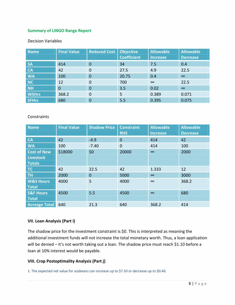
Summary of LINGO Range Report

Decision Variables

Name Final Value Reduced Cost Objective Coefficient

Allowable Increase

Allowable Decrease

SA 414 0 34 7.5 0.4

CA 42 0 27.5 4.9 22.5

WA 100 0 20.75 0.4 ∞

NC 12 0 700 ∞ 22.5

NH 0 0 3.5 0.02 ∞

WSHrs 368.2 0 5 0.389 0.071

SFHrs 680 0 5.5 0.395 0.075

Constraints

Name Final Value Shadow Price Constraint RHS

Allowable Increase

Allowable Decrease

CA 42 -4.9 0 414 42

WA 100 -7.40 0 414 100

Cost of New Livestock Totals

$18000 $0 20000 ∞ 2000

TC 42 22.5 42 1.333 12

TH 2000 0 5000 ∞ 3000

W&S Hours Total

4000 5 4000 ∞ 368.2

S&F Hours Total

4500 5.5 4500 ∞ 680

Acreage Total 640 21.3 640 368.2 414

VII. Loan Analysis (Part i)

The shadow price for the investment constraint is $0. This is interpreted as meaning the

additional investment funds will not increase the total monetary worth. Thus, a loan application

will be denied – it’s not worth taking out a loan. The shadow price must reach $1.10 before a

loan at 10% interest would be payable.

VIII. Crop Postoptimality Analysis (Part j)

1. The expected net value for soybeans can increase up to $7.50 or decrease up to $0.40.

9 | P a g e

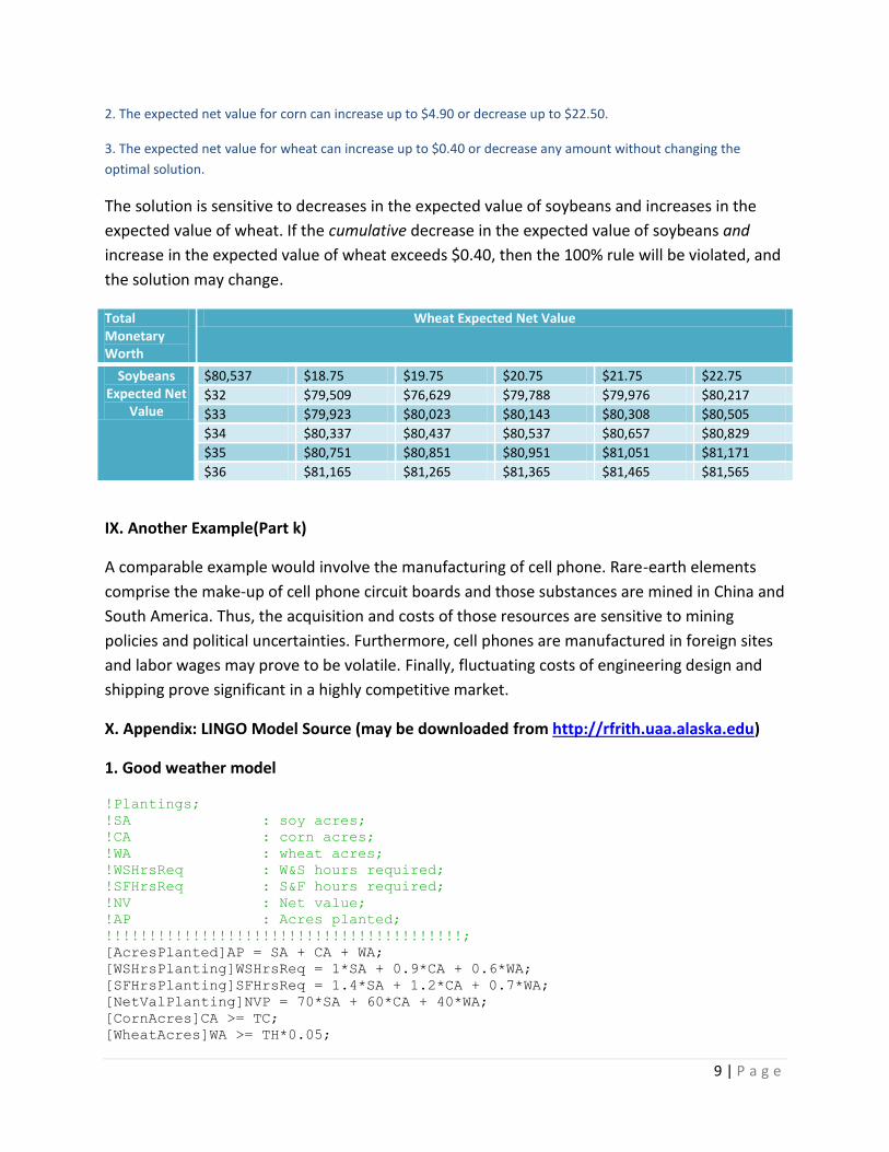
2. The expected net value for corn can increase up to $4.90 or decrease up to $22.50.

3. The expected net value for wheat can increase up to $0.40 or decrease any amount without changing the

optimal solution.

The solution is sensitive to decreases in the expected value of soybeans and increases in the

expected value of wheat. If the cumulative decrease in the expected value of soybeans and

increase in the expected value of wheat exceeds $0.40, then the 100% rule will be violated, and

the solution may change.

Total Monetary Worth

Wheat Expected Net Value

Soybeans Expected Net

Value

$80,537 $18.75 $19.75 $20.75 $21.75 $22.75

$32 $79,509 $76,629 $79,788 $79,976 $80,217

$33 $79,923 $80,023 $80,143 $80,308 $80,505

$34 $80,337 $80,437 $80,537 $80,657 $80,829

$35 $80,751 $80,851 $80,951 $81,051 $81,171

$36 $81,165 $81,265 $81,365 $81,465 $81,565

IX. Another Example(Part k)

A comparable example would involve the manufacturing of cell phone. Rare-earth elements

comprise the make-up of cell phone circuit boards and those substances are mined in China and

South America. Thus, the acquisition and costs of those resources are sensitive to mining

policies and political uncertainties. Furthermore, cell phones are manufactured in foreign sites

and labor wages may prove to be volatile. Finally, fluctuating costs of engineering design and

shipping prove significant in a highly competitive market.

X. Appendix: LINGO Model Source (may be downloaded from http://rfrith.uaa.alaska.edu)

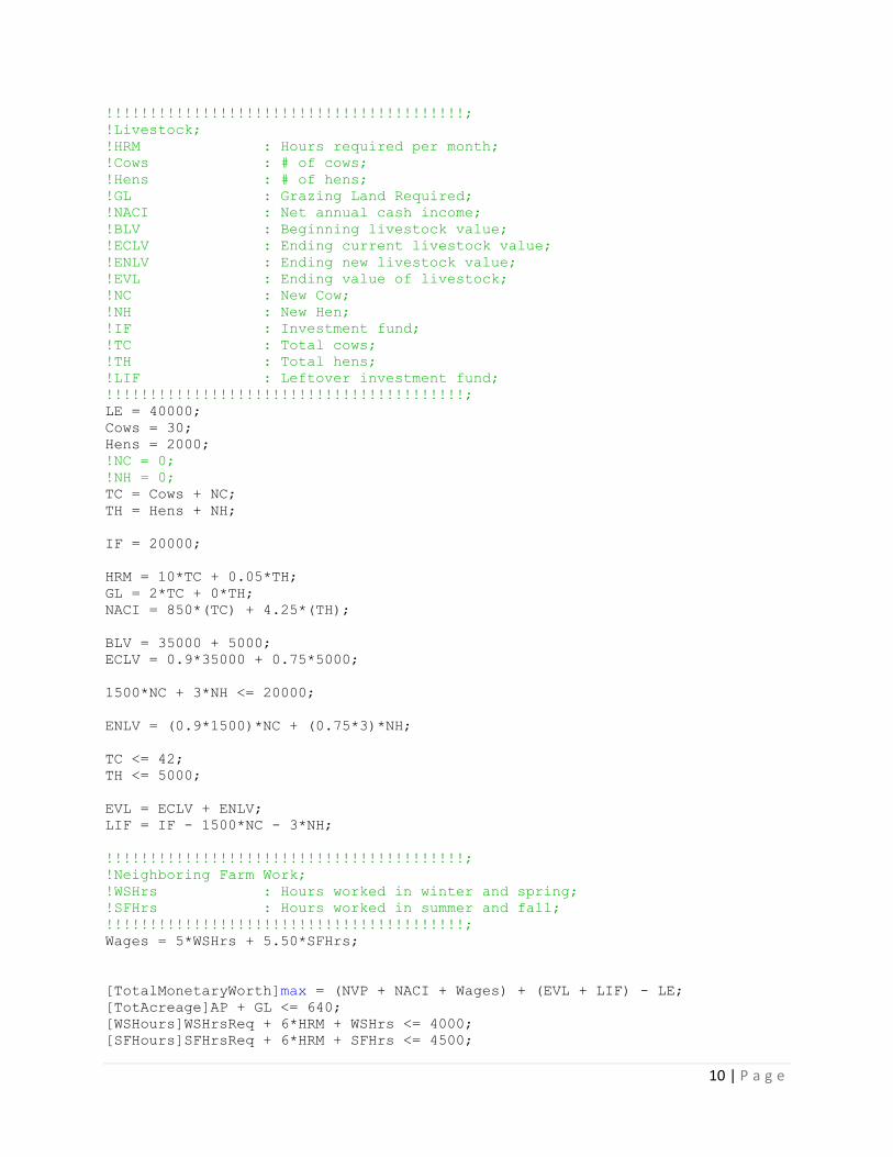
1. Good weather model

!Plantings;

!SA : soy acres;

!CA : corn acres;

!WA : wheat acres;

!WSHrsReq : W&S hours required;

!SFHrsReq : S&F hours required;

!NV : Net value;

!AP : Acres planted;

!!!!!!!!!!!!!!!!!!!!!!!!!!!!!!!!!!!!!!!!!;

[AcresPlanted]AP = SA + CA + WA;

[WSHrsPlanting]WSHrsReq = 1*SA + 0.9*CA + 0.6*WA;

[SFHrsPlanting]SFHrsReq = 1.4*SA + 1.2*CA + 0.7*WA;

[NetValPlanting]NVP = 70*SA + 60*CA + 40*WA;

[CornAcres]CA >= TC;

[WheatAcres]WA >= TH*0.05;

http://rfrith.uaa.alaska.edu/

10 | P a g e

!!!!!!!!!!!!!!!!!!!!!!!!!!!!!!!!!!!!!!!!!;

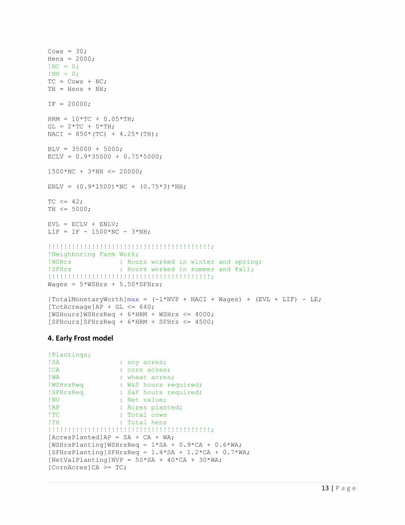
!Livestock;

!HRM : Hours required per month;

!Cows : # of cows;

!Hens : # of hens;

!GL : Grazing Land Required;

!NACI : Net annual cash income;

!BLV : Beginning livestock value;

!ECLV : Ending current livestock value;

!ENLV : Ending new livestock value;

!EVL : Ending value of livestock;

!NC : New Cow;

!NH : New Hen;

!IF : Investment fund;

!TC : Total cows;

!TH : Total hens;

!LIF : Leftover investment fund;

!!!!!!!!!!!!!!!!!!!!!!!!!!!!!!!!!!!!!!!!!;

LE = 40000;

Cows = 30;

Hens = 2000;

!NC = 0;

!NH = 0;

TC = Cows + NC;

TH = Hens + NH;

IF = 20000;

HRM = 10*TC + 0.05*TH;

GL = 2*TC + 0*TH;

NACI = 850*(TC) + 4.25*(TH);

BLV = 35000 + 5000;

ECLV = 0.9*35000 + 0.75*5000;

1500*NC + 3*NH <= 20000;

ENLV = (0.9*1500)*NC + (0.75*3)*NH;

TC <= 42;

TH <= 5000;

EVL = ECLV + ENLV;

LIF = IF - 1500*NC - 3*NH;

!!!!!!!!!!!!!!!!!!!!!!!!!!!!!!!!!!!!!!!!!;

!Neighboring Farm Work;

!WSHrs : Hours worked in winter and spring;

!SFHrs : Hours worked in summer and fall;

!!!!!!!!!!!!!!!!!!!!!!!!!!!!!!!!!!!!!!!!!;

Wages = 5*WSHrs + 5.50*SFHrs;

[TotalMonetaryWorth]max = (NVP + NACI + Wages) + (EVL + LIF) - LE;

[TotAcreage]AP + GL <= 640;

[WSHours]WSHrsReq + 6*HRM + WSHrs <= 4000;

[SFHours]SFHrsReq + 6*HRM + SFHrs <= 4500;

11 | P a g e

2. Drought model

!Plantings;

!SA : soy acres;

!CA : corn acres;

!WA : wheat acres;



!NV : Net value;


!TC : Total cows

!TH : Total hens

!!!!!!!!!!!!!!!!!!!!!!!!!!!!!!!!!!!!!!!!!;







!!!!!!!!!!!!!!!!!!!!!!!!!!!!!!!!!!!!!!!!!;

!Livestock;


!Cows : # of cows;

!Hens : # of hens;







!NC : New Cow;

!NH : New Hen;


!TC : Total cows;

!TH : Total hens;


!!!!!!!!!!!!!!!!!!!!!!!!!!!!!!!!!!!!!!!!!;

LE = 40000;

Cows = 30;

Hens = 2000;

TC = Cows + NC;

TH = Hens + NH;

IF = 20000;

HRM = 10*TC + 0.05*TH;

GL = 2*TC + 0*TH;

NACI = 850*(TC) + 4.25*(TH);

BLV = 35000 + 5000;

ECLV = 0.9*35000 + 0.75*5000;

1500*NC + 3*NH <= 20000;

ENLV = (0.9*1500)*NC + (0.75*3)*NH;

12 | P a g e

TC <= 42;

TH <= 5000;

EVL = ECLV + ENLV;

LIF = IF - 1500*NC - 3*NH;

!!!!!!!!!!!!!!!!!!!!!!!!!!!!!!!!!!!!!!!!!;




!!!!!!!!!!!!!!!!!!!!!!!!!!!!!!!!!!!!!!!!!;


[TotalMonetaryWorth]max = (-1*NVP + NACI + Wages) + (EVL + LIF) - LE;




3. Drought..Early Frost model

!Plantings;

!SA : soy acres;

!CA : corn acres;

!WA : wheat acres;



!NV : Net value;


!TC : Total cows

!TH : Total hens

!!!!!!!!!!!!!!!!!!!!!!!!!!!!!!!!!!!!!!!!!;







!!!!!!!!!!!!!!!!!!!!!!!!!!!!!!!!!!!!!!!!!;

!Livestock;


!Cows : # of cows;

!Hens : # of hens;







!NC : New Cow;

!NH : New Hen;


!TC : Total cows;

!TH : Total hens;


!!!!!!!!!!!!!!!!!!!!!!!!!!!!!!!!!!!!!!!!!;

LE = 40000;

13 | P a g e

Cows = 30;

Hens = 2000;

!NC = 0;

!NH = 0;

TC = Cows + NC;

TH = Hens + NH;

IF = 20000;

HRM = 10*TC + 0.05*TH;

GL = 2*TC + 0*TH;

NACI = 850*(TC) + 4.25*(TH);

BLV = 35000 + 5000;

ECLV = 0.9*35000 + 0.75*5000;

1500*NC + 3*NH <= 20000;

ENLV = (0.9*1500)*NC + (0.75*3)*NH;

TC <= 42;

TH <= 5000;

EVL = ECLV + ENLV;

LIF = IF - 1500*NC - 3*NH;

!!!!!!!!!!!!!!!!!!!!!!!!!!!!!!!!!!!!!!!!!;




!!!!!!!!!!!!!!!!!!!!!!!!!!!!!!!!!!!!!!!!!;


[TotalMonetaryWorth]max = (-1*NVP + NACI + Wages) + (EVL + LIF) - LE;




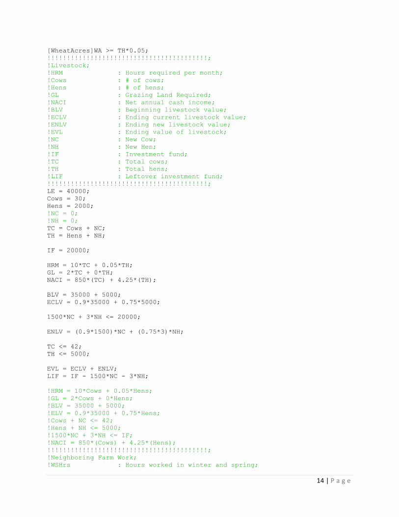
4. Early Frost model

!Plantings;

!SA : soy acres;

!CA : corn acres;

!WA : wheat acres;



!NV : Net value;


!TC : Total cows

!TH : Total hens

!!!!!!!!!!!!!!!!!!!!!!!!!!!!!!!!!!!!!!!!!;






14 | P a g e


!!!!!!!!!!!!!!!!!!!!!!!!!!!!!!!!!!!!!!!!!;

!Livestock;


!Cows : # of cows;

!Hens : # of hens;







!NC : New Cow;

!NH : New Hen;


!TC : Total cows;

!TH : Total hens;


!!!!!!!!!!!!!!!!!!!!!!!!!!!!!!!!!!!!!!!!!;

LE = 40000;

Cows = 30;

Hens = 2000;

!NC = 0;

!NH = 0;

TC = Cows + NC;

TH = Hens + NH;

IF = 20000;

HRM = 10*TC + 0.05*TH;

GL = 2*TC + 0*TH;

NACI = 850*(TC) + 4.25*(TH);

BLV = 35000 + 5000;

ECLV = 0.9*35000 + 0.75*5000;

1500*NC + 3*NH <= 20000;

ENLV = (0.9*1500)*NC + (0.75*3)*NH;

TC <= 42;

TH <= 5000;

EVL = ECLV + ENLV;

LIF = IF - 1500*NC - 3*NH;

!HRM = 10*Cows + 0.05*Hens;

!GL = 2*Cows + 0*Hens;

!BLV = 35000 + 5000;

!ELV = 0.9*35000 + 0.75*Hens;

!Cows + NC <= 42;

!Hens + NH <= 5000;

!1500*NC + 3*NH <= IF;

!NACI = 850*(Cows) + 4.25*(Hens);

!!!!!!!!!!!!!!!!!!!!!!!!!!!!!!!!!!!!!!!!!;



15 | P a g e


!!!!!!!!!!!!!!!!!!!!!!!!!!!!!!!!!!!!!!!!!;






!;

[NetInc]NI = NVP + NACI + Wages;

5. Flood model

!Plantings;

!SA : soy acres;

!CA : corn acres;

!WA : wheat acres;



!NV : Net value;


!TC : Total cows

!TH : Total hens

!!!!!!!!!!!!!!!!!!!!!!!!!!!!!!!!!!!!!!!!!;







!!!!!!!!!!!!!!!!!!!!!!!!!!!!!!!!!!!!!!!!!;

!Livestock;


!Cows : # of cows;

!Hens : # of hens;







!NC : New Cow;

!NH : New Hen;


!TC : Total cows;

!TH : Total hens;


!!!!!!!!!!!!!!!!!!!!!!!!!!!!!!!!!!!!!!!!!;

LE = 40000;

Cows = 30;

Hens = 2000;

!NC = 0;

!NH = 0;

TC = Cows + NC;

TH = Hens + NH;

16 | P a g e

IF = 20000;

HRM = 10*TC + 0.05*TH;

GL = 2*TC + 0*TH;

NACI = 850*(TC) + 4.25*(TH);

BLV = 35000 + 5000;

ECLV = 0.9*35000 + 0.75*5000;

1500*NC + 3*NH <= 20000;

ENLV = (0.9*1500)*NC + (0.75*3)*NH;

TC <= 42;

TH <= 5000;

EVL = ECLV + ENLV;

LIF = IF - 1500*NC - 3*NH;



!BLV = 35000 + 5000;

!ELV = 0.9*35000 + 0.75*Hens;

!Cows + NC <= 42;

!Hens + NH <= 5000;

!1500*NC + 3*NH <= IF;

!NACI = 850*(Cows) + 4.25*(Hens);

!!!!!!!!!!!!!!!!!!!!!!!!!!!!!!!!!!!!!!!!!;




!!!!!!!!!!!!!!!!!!!!!!!!!!!!!!!!!!!!!!!!!;






!;


6. Flood..Early Frost model

!Plantings;

!SA : soy acres;

!CA : corn acres;

!WA : wheat acres;



!NV : Net value;


!TC : Total cows

!TH : Total hens

!!!!!!!!!!!!!!!!!!!!!!!!!!!!!!!!!!!!!!!!!;

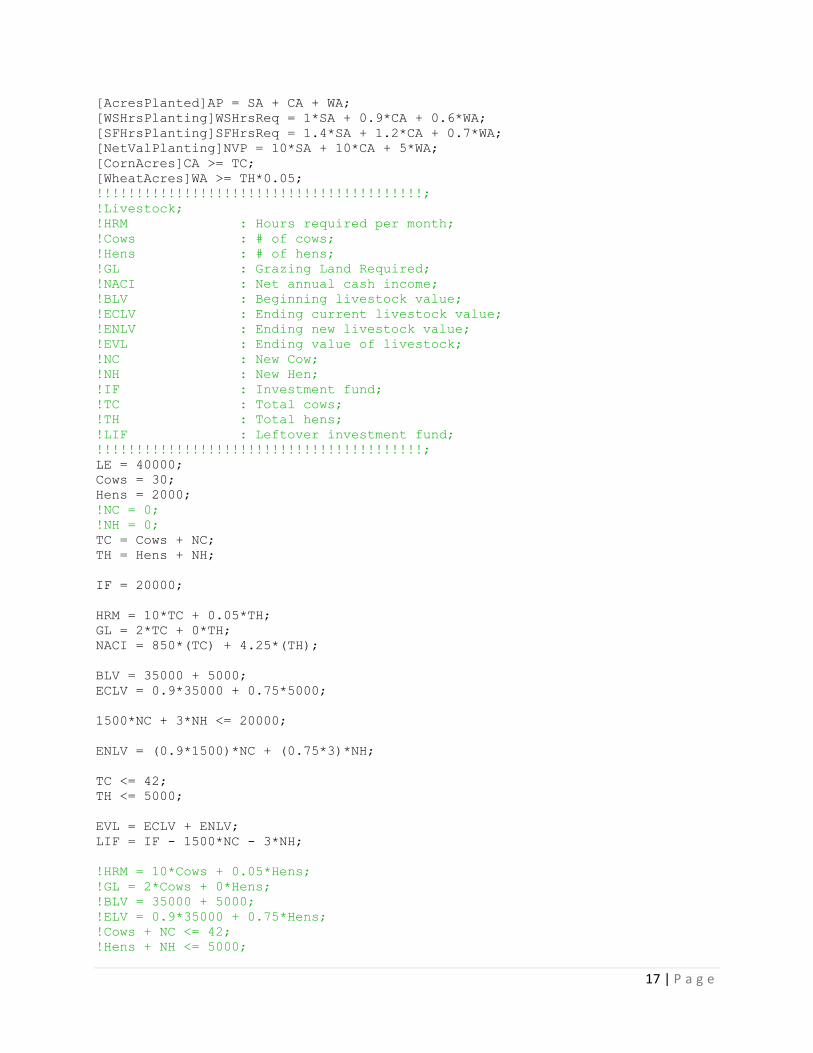
17 | P a g e







!!!!!!!!!!!!!!!!!!!!!!!!!!!!!!!!!!!!!!!!!;

!Livestock;


!Cows : # of cows;

!Hens : # of hens;







!NC : New Cow;

!NH : New Hen;


!TC : Total cows;

!TH : Total hens;


!!!!!!!!!!!!!!!!!!!!!!!!!!!!!!!!!!!!!!!!!;

LE = 40000;

Cows = 30;

Hens = 2000;

!NC = 0;

!NH = 0;

TC = Cows + NC;

TH = Hens + NH;

IF = 20000;

HRM = 10*TC + 0.05*TH;

GL = 2*TC + 0*TH;

NACI = 850*(TC) + 4.25*(TH);

BLV = 35000 + 5000;

ECLV = 0.9*35000 + 0.75*5000;

1500*NC + 3*NH <= 20000;

ENLV = (0.9*1500)*NC + (0.75*3)*NH;

TC <= 42;

TH <= 5000;

EVL = ECLV + ENLV;

LIF = IF - 1500*NC - 3*NH;



!BLV = 35000 + 5000;

!ELV = 0.9*35000 + 0.75*Hens;

!Cows + NC <= 42;

!Hens + NH <= 5000;

18 | P a g e

!1500*NC + 3*NH <= IF;

!NACI = 850*(Cows) + 4.25*(Hens);

!!!!!!!!!!!!!!!!!!!!!!!!!!!!!!!!!!!!!!!!!;




!!!!!!!!!!!!!!!!!!!!!!!!!!!!!!!!!!!!!!!!!;






!;


i, term ect 2014 - university of alaska systemrfrith.uaa.alaska.edu/opsres/project.pdf · r, joan...

Documents