“I hereby acknowledge that the scope and quality of this thesis is qualified for the

award of the Bachelor Degree of Electrical Engineering (Power System)”

Signature :____________________________________________

Name : AHMAD NOR KASRUDDIN BIN NASIR

Date : 11 NOVEMBER 2008

LINEAR QUADRATIC REGULATOR (LQR) CONTROLLER DESIGN

FOR DC MOTOR SPEED USING MATLAB APPLICATION

MOHD REDHA BIN RAJAB

This thesis is submitted as partial fulfillment of the requirements for the award of the

Bachelor of Electrical Engineering (Power Systems)

Faculty of Electrical & Electronics Engineering

Universiti Malaysia Pahang

NOVEMBER, 2008

“All the trademark and copyrights use herein are property of their respective owner.

References of information from other sources are quoted accordingly; otherwise the

information presented in this report is solely work of the author.”

Signature : _________________

Author : MOHD REDHA BIN RAJAB

Date : 11 NOVEMBER 2008

To my beloved mother, father, sisters, and brother

ACKNOWLEDGEMENT

In the name of Allah, The Most Loving and The Most Compassionate

In completing the thesis, I had receives helps from many people. They have

contributed towards my understanding and thoughts. In particular, I wish to express

my sincere appreciation to my supervisor, Mr. Ahmad Nor Kasruddin Bin Nasir, for

encouragement, guidance and critics. Further thanks and extended to my family, my

beloved parents, Rajab Bin Daud and Wan Halimah Binti Dollah for their advice and

support at various ossasions. I would like to give my sincere appreciation to all my

friends and others who have provided assistance at various occasions. Without them I

would not be here.

ABSTRACT This project is a about control system. To control the system, simulation and

experimental investigation into the development of LQR controller using

MATLAB/SIMULINK software. The simulation development of the LQR controller

with the mathematical model of DC motor. and trial and error method to tune the

system controller. The LQR parameter is to be tested with an actual motor also with

the LQR controller in MATLAB/SIMULINK software. Data acquisition is used In

order to implement the LQR controller from the software to the actual dc motor.

From this project, the result performance of the LQR controller is compared in term

of response and the assessment is presented

ABSTRAK

Projek ini adalah berkaitan system kawalan. Untuk system kawalan,

penyelidikan secara simulasi dan eksperimen dalam pembangunan pengawal LQR

mengunakan perisian MATLAB/SIMULINK. Pembangunan simulasi pengawal

LQR dengan model matematik dc motor dan kaedah cuba dan jaya untuk kawalan

system pengawal. Parameter pengawal LQR akan diuji dengan motor sebenar juga

dengan pengawal LQR mengunakan perisian MATLAB/SIMULINK. “ Data

acquisition card “ di gunakan bagi mengaplikasikan pengawal PID dari perisian

kepada motor DC sebenar. Dari projek ini, keputusan kecekapan dari pengawal PID

dibandingkan dari segi respon dan analisis dibentangkan.

TABLE OF CONTENTS

CHAPTER TITLE PAGE

TITLE PAGE i

STUDENT ADMITTANCE PAGE ii

DEDICATION iii

ACKNOWLEDGEMENT iv

ABSTRACT v

ABSTRAK vi

TABLE OF CONTENTS vii

LIST OF TABLES x

LIST OF FIGURES xi

LIST OF SYMBOLS xv

LIST OF APPENDICES xvi

1. INTRODUCTION

1.1 Project background 1

1.2 Objective 2

1.3 Scope 3

1.4 Problem Statement 3

2. LITERATURE REVIEW

2.1 Introduction 4

2.2 Introduction of Linear Quadratic Regulator 5

2.3 DC Motor 10

2.4 Mathematical Modeling 11

2.5 Data Acquisition Card 16

2.6 MATLAB 17

3. METHODOLOGY

3.1 System Description 20

3.2 Linear Quadratic Regulator System 21

3.2.1 MATLAB m-file 24

3.2.2 MATLAB of simulation 29

3.3 Data Acquisition System 31

3.3.1 PCI-1710HG 32

3.4 Real Time Target Setup 40

3.4.1 Installation and Configuration 42

3.4.2 Real Time Application 47

3.5 Driver 62

3.5.1 Geckodrive G340 62

3.5.2 Alternative Driver IR2109 63

3.6 Hardware used in this project 64

3.7 Flow Diagram for System 68

4. RESULT AND DISCUSSION 69

4.1 Controller Design 69

4.2 Simulation without LQR Controller 70

4.3 Simulation with LQR Controller 71

4.4 Experiment without LQR controller 76

4.5 Experiments with LQR Controller 77

5. CONCLUSIONS AND RECOMMENDATIONS 80

5.1 Introduction 80

5.2 Assessment of design 81

5.3 Strength and Weakness 82

5.4 Recommendations 82

6. REFERENCES 83

7. APPENDICES 85

LIST OF TABLES

TABLE NO. TITLE PAGE

4.1 Data analysis simulink of the system 73 4.2 Data analysis Experiment without LQR 75

LIST OF FIGURES

FIGURE NO. TITLE PAGE 2.1 Optimal Regulator System 6 2.2 Schematic diagram of a DC motor 11

2.3 Block diagram of the open-loop Permanent-magnet DC motor 14

2.4 Block diagram of the open-loop servo actuated by permanent-magnet DC motor 14

2.5 MATLAB screen 18 3.1 Block Diagram of the System 21 3.2 Graf for m-file simulation 25 3.3 LQR simulink block. . 26 3.4 Subsystem simulink block. 27 3.5 Graf for Simulink block 27 3.6 Pin Assignment 33 3.7 Block Diagram of PCI-1710HG 34 3.8 PCI-1710HG Installation Flow Chart 36 3.9 Required Products of Real Time Windows Target 38

3.10 Simulink Model rtvdp.mdl 42 3.11 Output Signal rtvdp.mdl 43 3.12 Create a new model 44 3.13 Empty Simulink mode 45 3.14 Block Parameters of Signal Generator 46 3.15 Board Test OK Dialog 47 3.16 Block Parameters of Analog Output 48 3.17 Scope Parameters Dialog Box 49 3.18 Scope Window 50 3.19 Scope Properties: axis 1 51 3.20 Completed Simulink Block Diagram 52 3.21 Configuration Parameters – Solver 56 3.22 Configuration Parameters – Hardware Implementation 57 3.23 System Target File Browser 57 3.24 Configuration Parameters – Real-Time Workshop 58 3.25 Connect to target from the Simulation menu 60 3.26 Geckodrive G340 Block Diagram 63

3.27 Typical connections for IR2109 64 3.28 Data Acuisation Card (PCI-1710HG) 64

3.29 Industrial Wiring Terminal Board with

CJC Circuit (PCLD-8710) 65

3.30 Personal computer 65

3.31 Geckodrive G340 66

3.32 Alternative Driver (IR2109) 66

3.33 Power Supply 66

3.34 Oscilloscope 66

3.35 Litton - Clifton Precision Servo DC Motor JDH-2250 67 3.36 Flow Diagram for System 68

4.1 Simulink Block of the System 70

4.2 Output of dc Motor without LQR Controller 71

4.3 LQR simulink block system 72

4.4 Subsystem simulink block 72

4.5 Output of DC Motor with LQR Controller 73

4.6 Simulink Block of Experiment without LQR 74

4.7 Velocity Estimation 76 4.8 Complete Simulink Block of the Experiment 77 4.9 Velocity Decoder Subsystem Simulink Block 78

LIST OF SYMBOLS

D - duty cycle

T - period

TL - load torque

Өr - angle

ωr - rotor angular displacement

ia - armature current

Ea - Induced emf

ka - back emf / torque constant

ra - armature resistance

La - armature inductance

J - moment of inertia

BBm - viscous friction coefficient

Tviscous - viscous friction torque

ua - armature voltage

Ts - settling time

Z - damping ratio

wn - natural frequency

clf - clear graph on screen

Tss - transfer state-space

LIST OF APPENDICES

APPENDIX TITLE PAGE

A Block Diagram of the System Controller 85

B LQR simulink block 86

C Subsystem simulink block 87

D Simulink Block of Experiment without LQR 88 E Complete Simulink Block of the Experiment 89

CHAPTER 1

INTRODUCTION

1.1 Background of Project

Control engineering is one subject which is perceived as being the most

theoretical and most difficult to understand. In industries, application of motor

control system is important to operation some process. An average home in

Malaysia uses a dozen or more electric motors. In some application the DC motor is

required to maintain its desired speed when load is applied or disturbance occur.

This kind of system can be controlled using PID, Fuzzy, LQR and other more.

In this project, Linear Quadratic Regulator (LQR) controller is introducing in

order to control the DC motor speed as we required. MATLAB/SIMULINK is used

to design and tune the LQR controller and be simulated to mathematical model of the

DC motor. From the simulation the LQR controller in MATLAB/SIMULINK is

interfaced with the actual DC motor using a data acquisition card.

The Linear Quadratic Regulator (LQR) controller is a new method of

controlling the motor. Linear Quadratic Regulator (LQR) is theory of optimal control

concerned with operating a dynamic system at minimum cost.

1.2 Objective of project

The objectives of this project are:

i. To control DC motor speed using LQR controller.

ii. To observe the performance comparison between experiment and simulation

result.

iii. To design the LQR controller and tune it using MATLAB/SIMULINK.

1.3 Scope of Project

The main scope of this project is to build control system for control DC motor.

i. Design and produce the simulation of the LQR controller.

ii. To Implement LQR controller to actual DC motor.

iii. The comparison of the simulation result with the actual DC motor

1.4 Problem Statement

Problem encountered:

i. Control DC motor speed

ii. Interface DC motor with MATLAB simulink diagram

iii. To acquire data from the DC motor.

Solutions:

i. Use LQR controller as a control DC motor

ii. Implementation of DAQ card to the control board

iii. Use encoder from the DC motor to the control board.

CHAPTER 2

LITERATURE REVIEW

2.1 Introduction

This chapter will explain the literature study that is related to the project

task. The information get from several sources such as websites, journals, books,

magazines, handout and others.

2.2 Introduction of Linear Quadratic Regulator

The linear quadratic regulator (LQR) is a well-known design technique that

provides practical feedback gains. For the derivation of the linear quadratic regulator,

assume that the plant to be written in state-space form as:

(1) BuAxa +='

And that all of the n states x are available for the controller. The feedback

gain is a matrix K of the optimal control vector

)()( tKxtu −= (2)

so as to minimize the performance index

(3) ∫∞

⋅+⋅=0

)( dtRuuQxxJ

Where Q is a positive-definite (or positive-semidefinite) Hermitian or real

symmetric matrix and R is a positive-definite Hermitian or real symmetric matrix.

Note that the second term on the right-hand side of the Equation 3 accounts for the

expenditure of the energy of the control signals. The matrices Q and R determine the

relative importance of the error and the expenditure of this energy. In this problem,

assume that the control vector is unconstrained. )(tu

As will be seen later, the linear control law given by Equation (2) is the

optimal control law. Therefore, if the unknown elements of the matrix K are

determined so as to minimize performance index, then is optimal for

any initial state x(0). The block diagram showing the optimal configuration is shown

in Figure below :

Figure 2.1: Optimal Regulator System

Now let solve the optimization problem. Substituting Equation 2 into Equation 1

(4) xBKABKxAxx )(' −=−=

In the following derivations, assume that the matrix is stable, or that

the eigenvalues of have negative real parts.

Substituting Equation 2 into Equation 3 yields :

∫∞

⋅⋅+⋅=0

)( dtRKxKxQxxJ

(5) ∫∞

⋅+⋅=0

))(( dtxRKKQx

Let set,

)(

)(Pxxdt

dxRKKQx⋅

−=⋅+⋅ (6)

Where P is a positive-definite Hermitian or real symmetric matrix. Then obtain

( )[ ]xBKAPPBKAxPxxPxxxRKKQx )()( −+⋅−−=⋅−⋅−=⋅+⋅ (7)

Comparing both sides of this last equation and noting that this equation must

hold true for any x, it require that

)()()( RKKQBKAPPBKA ⋅+−=−+⋅− (8)

It can be proved that if is a stable matrix, there exists a positive-

definite matrix P that satisfies Equation 8. Hence the next procedure is to determine

the elements of P from Equation 8 and see if it is positive definite. (Note that more

than one matrix P may satisfy this equation. If the system is stable, there always

exists one-positive matrix P to satisfy this equation. This means that, if to solve this

equation and find one positive-definite matrix P, the system is stable. Other P

matrices that satisfy this equation are not positive definite and must be discarded.)

The performance index J can be evaluated as

∫ (9) ∞

⋅−=⋅+⋅=0

))(( PxxdtxRKKQxJ

Since all eigenvalues of are assumed to have negative real parts, it have

x(∞) 0. Therefore, J can be obtain

)0()0( PxxJ ⋅= (10)

Thus, the performance index J can be obtained in terms of the initial

condition x(0) and P. To obtain the solution to the quadratic optimal control problem,

proceed as follows: Since R has been assumed to be a positive-definite Hermitian or

real symmetric matrix, it can be write

TTR ⋅= (11)

Where T is a nonsingular matrix. Then Equation 8 can be written as

0)()( =⋅⋅++−+⋅− TKTKQBKAPBKA (12)

Which can be rewritten as:

[ ] [ ] 00()( 111 =+⋅−⋅⋅−⋅⋅⋅−++⋅ −−− QPBPBRPBTTKPBTTKPAPA

(13)

The minimization of J with respect to K requires the minimization of

[ ] [ ]xPBTTKPBTTKx ⋅⋅−⋅⋅⋅− −− 11 )()( (14)

With respect to K. Since this last expression is nonnegative, the minimum

occurs when it is zero, or when

(15) PBTTK ⋅⋅= −1)(

Hence

(16)

PBRPBTTK ⋅=⋅⋅= −−− 111 )(

Equation 16 gives optimal matrix K. Thus, the optimal control law to the

quadratic optimal control problem when the performance index is given by Equation

3 is linear and is given by

) (17) ()()( 1 tPxBRtKxtu ⋅=−= −

The matrix P in Equation 16 must satisfy Equation 4 or the following reduced

equation:

(18) 01 =+⋅−+⋅ − QPBPBRPAPA

Equation 18 is called the reduced-matrix Riccati equation. The design steps may be

stated as follows:

1. Solve Equation 18, the reduced-matrix Riccati equation, for the matrix P.

2. [If a positive-definite matrix P exists (certain systems may not have a

positive-definite matrix P), the system is stable, or matrix is stable.]

3. Substitute this matrix P into Equation 16. The resulting matrix K is the

optimal matrix.

Note that if the matrix is stable, the present method always gives the

correct result. Finally, note that if the performance index is given in terms of the

output vector rather than the state vector, that is

(19) ∫∞

⋅+⋅=0

)dtRuuQyyJ

Then, the index can be modified by using the output equation

(20) Cxy =

To

(21) ∫∞

⋅+⋅⋅=0

)( dtRuuQCxCxJ

and the design steps presented in this part can be applied to obtain optimal matrix K.

2.3 DC Motor

DC motors consist of one set of coils, called an armature, inside another set

of coils or a set of permanent magnets, called the stator. Applying a voltage to the

coils produces a torque in the armature, resulting in motion. It design to run on DC

electric power which uses electrical energy and produce mechanical energy. There

are two types of DC motor which are brush and brushless types, in order to create an

oscillating AC current from the DC source and internal and external commutation is

use respectively. So they are not purely DC machines in a strict sense .

A brushless DC motor (BLDC) is a synchronous electric motor which is

powered by direct-current electricity (DC) and which has an electronically controlled

commutation system, instead of a mechanical commutation system based on brushes.

In such motors, current and torque, voltage and rpm are linearly related. BLDC

motors offer several advantages over brushed DC motors, including higher efficiency

and reliability, reduced noise, longer lifetime (no brush erosion), elimination of

ionizing sparks from the commentator, and overall reduction of electromagnetic

interference (EMI).

With no windings on the rotor, they are not subjected to centrifugal forces,

and because the electromagnets are located around the perimeter, the electromagnets

can be cooled by conduction to the motor casing, requiring no airflow inside the

motor for cooling. BLDC's main disadvantage is higher cost, which arises from two

issues. First, BLDC motors require complex electronic speed controllers to run..

2.4 Mathematical Modeling

Figure 2.2: Schematic diagram of a DC motor

To design the control algorithm, first find the transfer function to develop the

block diagrams of the open and close loop systems. These transfer function are

obtained using the differential equation that descried the system dynamic.

Kirchhoff’s voltage is use to map the armature circuitry dynamic of the motor.

aa

ra

aa

a

ai uLL

ki

Lr

dtdi 1

+−−= ϖ

Using Newton’s 2nd law

∑ ==dtdJJT ωαr

rr

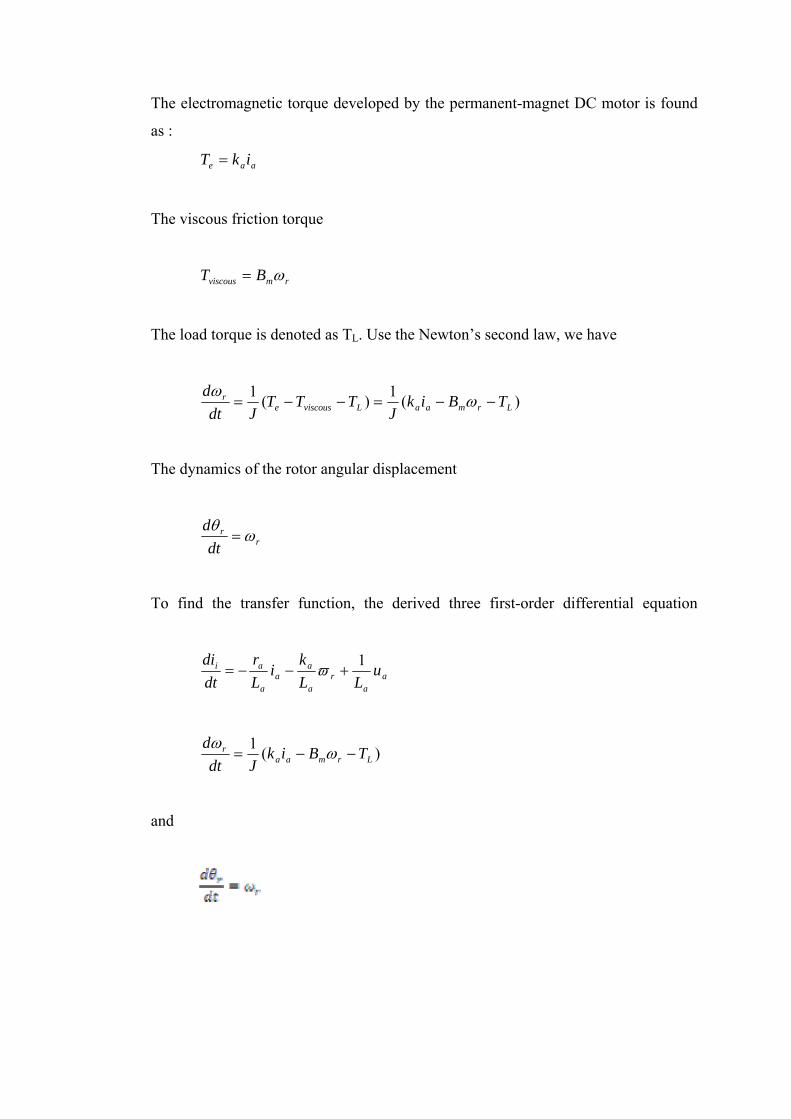
The electromagnetic torque developed by the permanent-magnet DC motor is found

as :

aae ikT =

The viscous friction torque

rmviscous BT ω=

The load torque is denoted as TL. Use the Newton’s second law, we have

)(1)(1LrmaaLviscouse

r TBikJ

TTTJdt

d−−=−−= ω

ω

The dynamics of the rotor angular displacement

rr

dtd

ωθ

=

To find the transfer function, the derived three first-order differential equation

aa

ra

aa

a

ai uLL

ki

Lr

dtdi 1

+−−= ϖ

)(1Lrmaa

r TBikJdt

d−−= ω

ω

and

Using the Laplace operator

)(1)()( suL

sLk

siLr

s aa

ra

aa

a

a +−=⎟⎟⎠

⎞⎜⎜⎝

⎛+ ω

)(1)(1)( sTJ

sikJ

sJ

Bs Laar

m −=⎟⎠⎞

⎜⎝⎛ + ω

From the transfer function, the block diagram of the permanent-magnet DC motor is

illustrated by figure 2.3

Figure 2.3: Block diagram of the open-loop permanent-magnet DC motor

Figure 2.4: Block diagram of the open-loop servo actuated by permanent-magnet DC

motor

From equation ( to find matrix)

aa

ra

aa

a

ai uLL

ki

Lr

dtdi 1

+−−= ϖ

)(1Lrmaa

r TBikJdt

d−−= ω

ω

the dynamic equations in state-space form are the following:

vLi

JB

Jk

Lk

Lr

idtd

ma

a

a

a

a

⎥⎥

⎦

⎤

⎢⎢

⎣

⎡+⎥

⎦

⎤⎢⎣

⎡

⎥⎥⎥⎥

⎦

⎤

⎢⎢⎢⎢

⎣

⎡

−

−−=⎥

⎦

⎤⎢⎣

⎡

0

1

θθ

[ ] ⎥⎦

⎤⎢⎣

⎡=

θθ

i10

DuCxyBuAxx

+=+='

⎥⎥⎥⎥

⎦

⎤

⎢⎢⎢⎢

⎣

⎡

−

−−=

JB

JK

Lk

Lr

Ama

a

a

a

a

⎥⎥

⎦

⎤

⎢⎢

⎣

⎡=

0

1LB

[ 10=C ] 0=D

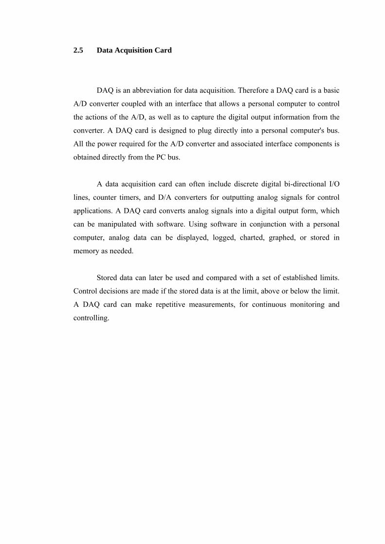
2.5 Data Acquisition Card

DAQ is an abbreviation for data acquisition. Therefore a DAQ card is a basic

A/D converter coupled with an interface that allows a personal computer to control

the actions of the A/D, as well as to capture the digital output information from the

converter. A DAQ card is designed to plug directly into a personal computer's bus.

All the power required for the A/D converter and associated interface components is

obtained directly from the PC bus.

A data acquisition card can often include discrete digital bi-directional I/O

lines, counter timers, and D/A converters for outputting analog signals for control

applications. A DAQ card converts analog signals into a digital output form, which

can be manipulated with software. Using software in conjunction with a personal

computer, analog data can be displayed, logged, charted, graphed, or stored in

memory as needed.

Stored data can later be used and compared with a set of established limits.

Control decisions are made if the stored data is at the limit, above or below the limit.

A DAQ card can make repetitive measurements, for continuous monitoring and

controlling.

2.6 MATLAB

MATLAB started as an interactive program for doing matrix calculations and

has now grown to a high level mathematical language that can solve integrals and

differential equations numerically and plot a wide variety of two and three

dimensional graphs. In this subject you will mostly use it interactively and also

create MATLAB scripts that carry out a sequence of commands. MATLAB also

contains a programming language that is rather like Pascal.

The first version of Matlab was produced in the mid 1970s as a teaching tool.

The vastly expanded Matlab is now used for mathematical calculations and

simulation in companies and government labs ranging from aerospace, car design,

signal analysis through to instrument control & financial analysis. Other similar

programs are Mathematica and Maple. Mathematica is somewhat better at symbolic

calculations but is slower at large numerical calculations.Recent versions of Matlab

also include much of the Maple symbolic calculation program

In this lab you will cover the following basic things:

i. using Matlab as a numerical calculator

ii. entering row vectors and column vectors

iii. entering matrices

iv. forming matrix and vector products

v. doing matrix products, sums etc

vi. using Matlab to solve linear equations

vii. Matlab functions that operate on arrays

viii. Plotting basic graphs using Matlab.

To get started MATLAB

When the computer has started go through the following steps in the different menus

• Look for the Network Applications folder and double click on that

• Within this you will see a little icon for Matlab – double click on that

Within about 30 seconds Matlab will open (you may get a little message box about

ICA

applications – just click OK on this)

You should now see a screen like the picture below

Figure 2.5: MATLAB screen

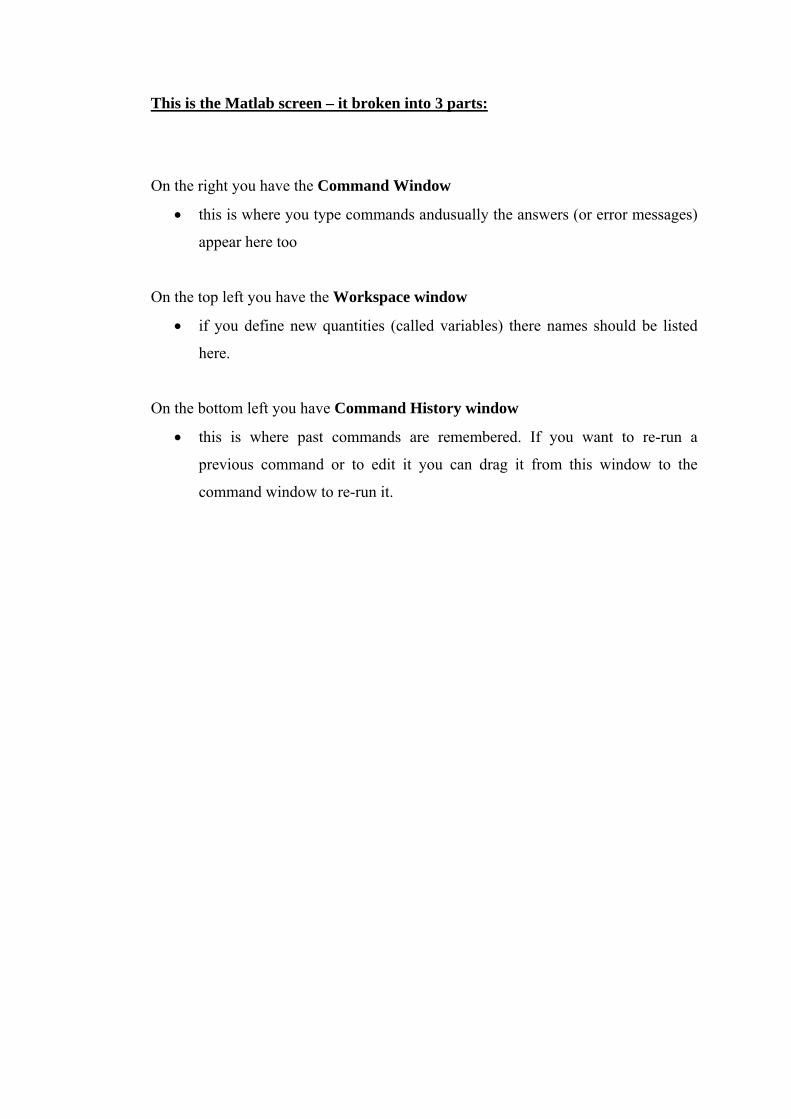
This is the Matlab screen – it broken into 3 parts:

On the right you have the Command Window

• this is where you type commands andusually the answers (or error messages)

appear here too

On the top left you have the Workspace window

• if you define new quantities (called variables) there names should be listed

here.

On the bottom left you have Command History window

• this is where past commands are remembered. If you want to re-run a

previous command or to edit it you can drag it from this window to the

command window to re-run it.

CHAPTER 3

METHODOLOGY

3.1 System Description

The block diagram is shown in Figure 3.1 is a system for my project. It divide

of 2 main block ( PC and Motor ) that are connected through a driver and supplied by

a power supply. Driver it also gives supplied power. The control algorithm is builder

in the Matlab/Simulink software and compiled with Real-Time Window Target. The

Real-Time Window Target Toolbox include an analog input and analog output that

provide connection between the data acquisition card ( PCI-1710HG ) and the

simulink model. For example, the speed of the DC motor could be controlled by

supplying certain voltage and frequency from signal generator block to the analog

output in Simulink. From the analog input, the square received is displayed in a

scope. The square wave pulse then is derived using the velocity equation to get the

velocity of the DC motor speed. The speed acquired and the signal send can create a

closed loop system with Linear Quadratic Regulator (LQR) controller to control the

speed of the DC motor.

PC

(SIMULATION)

DAQ CARD

MOTOR

ENCORDER

DRIVER

SPEED MEASURE

Figure 3.1 Block Diagram of the System

3.2 Linear Quadratic Regulator System

A description of the linear Quadratic Regulator ( LQR ) system considered in

this work is show in equation below:

01 =+⋅−+⋅ − QPBPBRPAPA TT

This equation is called the Algebraic Ricacati Equation (ARE). For a symmetric

positive-definite matrix P. The regulator gain K is given by

. PBRPBTTK T ⋅=⋅⋅= −−− 111 )(

To development LQR system, first we should find state-space from the transfer

function below: This equation get from mathematical modeling of DC motor .

aa

ra

aa

a

ai uLL

ki

Lr

dtdi 1

+−−= ϖ

)(1Lrmaa

r TBikJdt

d−−= ω

ω

the dynamic equations in state-space form are the following:

vLi

JB

Jk

Lk

Lr

idtd

ma

a

a

a

a

⎥⎥

⎦

⎤

⎢⎢

⎣

⎡+⎥

⎦

⎤⎢⎣

⎡

⎥⎥⎥⎥

⎦

⎤

⎢⎢⎢⎢

⎣

⎡

−

−−=⎥

⎦

⎤⎢⎣

⎡

0

1

θθ

[ ] ⎥⎦

⎤⎢⎣

⎡=

θθ

i10

DuCxyBuAxx

+=+='

⎥⎥⎥⎥

⎦

⎤

⎢⎢⎢⎢

⎣

⎡

−

−−=

JB

JK

Lk

Lr

Ama

a

a

a

a

⎥⎥

⎦

⎤

⎢⎢

⎣

⎡=

0

1LB

[ 10=C ] 0=D

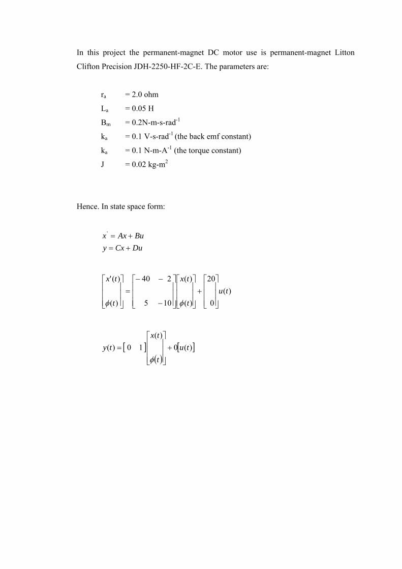
In this project the permanent-magnet DC motor use is permanent-magnet Litton

Clifton Precision JDH-2250-HF-2C-E. The parameters are:

ra = 2.0 ohm

La = 0.05 H

Bm = 0.2N-m-s-rad-1

ka = 0.1 V-s-rad-1 (the back emf constant)

ka = 0.1 N-m-A-1 (the torque constant)

J = 0.02 kg-m2

Hence. In state space form:

DuCxyBuAxx

+=+='

)(0

20

)(

)(

105

240

)(

)('tu

t

tx

t

tx

⎥⎥⎥

⎦

⎤

⎢⎢⎢

⎣

⎡+

⎥⎥⎥

⎦

⎤

⎢⎢⎢

⎣

⎡

⎥⎥⎥

⎦

⎤

⎢⎢⎢

⎣

⎡

−

−−=

⎥⎥⎥

⎦

⎤

⎢⎢⎢

⎣

⎡

φφ

[ ]( )

[ ])(0)(

10)( tut

txty +

⎥⎥⎥

⎦

⎤

⎢⎢⎢

⎣

⎡=

φ

3.2.1 MATLAB m-file

To find value of K, MATLAB m-file was used. Matlab m-file is show below:

clc

clf

ra=2.0;

La=0.05;

J=0.02;

Kg=0.1;

Bm=0.2;

Ka=0.1;

A=[-ra/La -Ka/La;Ka/J -Bm/J ] % system matrik

B=[1/La ; 0]

C=[0 1]

D=[0]

[numg,deng] = ss2tf(A,B,C,D)

'Uncompensated G(s)'

G=tf(numg,deng)

r1=roots(deng)

pos=5

Ts=0.58

z=(-log(pos/100))/(sqrt(pi^2+(log(pos/100))^2));

wn=4/(z*Ts);

[num,den]=ord2(wn,z);

r=roots(den)

poles=[r(1);r(2)]

characteristiceqdesired=poly(poles)

[Ac Bc Cc Dc]=tf2ss(numg,deng);

P=[0 1;1 0]

Ap=inv(P)*Ac*P;

Bp=inv(P)*Bc;

Cp=Cc*P;

Dp=Dc;

Q=[1 0 ;0 1];

R=1;

Kp=lqr(Ap,Bp,Q,R)

Apnew=Ap-Bp*Kp;

Bpnew=Bp;

Cpnew=Cp;

Dpnew=Dp;

[numt,dent]=ss2tf(Apnew,Bpnew,Cpnew,Dpnew);

'T(s)'

T=tf(numt,dent)

poles=roots(dent)

Tss=ss(Apnew,Bpnew,Cpnew,Dpnew)

t = 0:0.01:3;

G=4.1;

Tss=Tss*G;

step(Tss,t)

axis([0 2 0 1.4]);

title('Compensated Step Response')