i a study of the strain signals behaviour ng jun …umpir.ump.edu.my/8431/1/cd8118_@_51.pdf ·...

i

A STUDY OF THE STRAIN SIGNALS BEHAVIOUR

NG JUN PIN

Thesis submitted in fulfillment of the requirements

for the award of the degree of

Bachelor of Mechanical Engineering

Faculty of Mechanical Engineering

UNIVERSITI MALAYSIA PAHANG

JUNE 2013

vii

ABSTRACT

This study presents the study of strain signals behavior. In this study, the strain signal of

helical spring at different value of excitations is used to study the signals behavior.

When a vehicle was driven on any road surfaces, the significant load is transmitted to

the helical spring to absorb loads. The load values were varied according to the type of

the road surfaces. The signals were analyzed by statistical analysis and frequency-time

domain. Signals are classified based on the value of the statistical parameter. The

signals are used to predict fatigue damage of the helical spring. From the result obtained,

the unpaved road signals consist of higher peak shocks. It exhibited higher statistical

value compared to the signals obtained from university road and highway. These feature

increased the fatigue damage potential of the helical spring. The finite element analysis

of helical spring was performed by MSC Nastran with Patran software. The finite

element model was analysed using the linear elastic stress. Finally, the result obtained

and signals are employed to test the fatigue damage of helical spring. Strain-life model

which are Coffin-Manson, SWT and Morrow model are used to predict the fatigue

damage of helical spring. The obtained result indicated that unpaved road has the

highest fatigue damage followed by university road and highway.

viii

ABSTRAK

Kajian ini membentangkan sifat isyarat terikan. Dalam kajian ini, isyarat terikan spring

heliks dikaji dengan mengenakan daya yang berbeza. Ketika kenderaan dipandu melalui

permukaan jalan yang berbeza, beban kereta akan mengenakan daya pada heliks spring

kereta untuk menyerap beban. Permukaan jalan yang berbeza akan menghasilkan isyarat

terikan yang berlainan. Isyarat terikan spring heliks yang diperoleh akan dianalisis

dengan analisis statistik dan domain frekuensi masa. Oleh itu, isyarat terikan spring

akan dikelaskan berdasarkan nilai parameter statistik. Isyarat ini juga digunakan untuk

meramalkan kerosakan lesu spring heliks. Daripada keputusan yang diperoleh, isyarat

terikan spring heliks jalan tidak berturap terdiri daripada kejutan puncak yang lebih

tinggi. Selain itu, ia juga mempunyai nilai statistik yang lebih tinggi berbanding dengan

isyarat terikan spring heliks yang diperoleh dari jalan university dan jalan raya. Ciri ini

akan meninggikan potensi kerosakan lesu pada spring heliks. Analisis unsur terhingga

dijalankan dengan menggunakan MSC Nastran dan Patran. Pendekatan linear elastik

digunakan untuk menjalankan analisis tersebut. Keputusan analisis unsur yang

diperoleh dan isyarat terikan diperlukan untuk menghasilkan plot kontor kerosakan pada

kritikal tempat spring heliks. Model Coffin-Manson, SWT dan Morrow digunakan

untuk meramalkan kerosakan lesu pada spring heliks. Dari hasil keputusan didapati

bahawa jalan yang tidak berturap menunjukkan kerosakan tertinggi, diikuti dengan jalan

university dan akhirnya lebuh raya.

ix

TABLE OF CONTENTS

Page

SUPERVISOR’S DECLARATION iii

STUDENT’S DECLARATION iv

ACKNOWLEDGEMENTS vi

ABSTRACT vii

ABSTRAK viii

TABLE OF CONTENTS ix

APPENDICES xi

LIST OF TABLES xii

LIST OF FIGURES xiii

LIST OF SYMBOLS xvi

LIST OF ABBREVIATION xvii

CHAPTER 1 INTRODUCTION 1

1.0 Background Of Study 1

1.1 Problem Statement 2

1.2 Objectives 2

1.3 Scopes 2

CHAPTER 2 LITERATURE REVIEW 4

2.1 Introduction 4

2.2 Signal 4

2.3 Signal Types 5

2.4 Signal Statistical Parameter 8

2.5 Frequency Domain Analysis 10

2.5.1 Fourier Transform 10

2.5.2 Discrete Fourier Transform 11

2.5.3 Short-Time Fourier Transform 11

x

2.6 Total Fatigue Damage 12

2.6.1 Strain-Life Based Approach (ε-N) 13

2.6.2 Mean Stress Effects 16

CHAPTER 3 METHODOLOGY 19

3.1 Introduction 19

3.2 Solid Modelling of Helical Spring 21

3.3 Simulation of Helical Spring 22

3.3.1 Linear Elastic Stress Analysis 22

3.3.2 Statistical and FFT Analysis 25

3.3.3 Fatigue Analysis 26

CHAPTER 4 RESULTS AND DISCUSSION 28

4.1 Introduction 28

4.2 Strain Signal 28

4.3 Statistical Parameter Analysis 31

4.4 FFT Analysis 32

4.5 Fatigue Analysis 35

CHAPTER 5 CONCLUSION AND RECOMMENDATIONS 41

5.1 Conclusion 41

5.2 Recommendation 42

REFERENCES 44

xi

APPENDICES

A Strain gauge is glued on helical spring 47

B National Instrument (NI) is connected from strain

gauge to laptop

48

C Setup of strain signal experiment 49

D Road profile 50

E Gantt Chart for Final Year Project 1 52

F Gantt Chart for Final Year Project 2 53

xii

LIST OF TABLES

Table No. Title Page

3.1 Helical spring specification 21

3.2 Material properties of spring steel 23

4.1 The statistical values for different road profiles

32

4.2 Result of fatigue damage 36

xiii

LIST OF FIGURES

Figure No. Title Page

2.1 Sampling a continuous function of time at regular

intervals

4

2.2 The Gaussian distribution 5

2.3 Typical signal classification 8

2.4 Strain-life curve 14

2.5 Effect of mean stress on Strain-Life curve 16

2.6 Effect of mean stress on Strain-Life curve ( Morrow 17

correction)

3.1 Flowchart of Research Methodology 20

3.2 Helical spring in CATIA V5 software 22

3.3 Helical spring with 16829 nodes and 8523 elements 23

3.4 Stress distribution for static loading 24

3.5 Displacement distribution of static loading 25

3.6 FFT analysis using DASYLab 26

3.7 Fatigue life assessment using nCode DesignLife 27

4.1 Strain signal of highway 29

4.2 Strain signal of university road 30

4.3 Strain signal of unpaved road 30

xiv

4.4 FFT of highway 33

4.5 FFT of university road 33

4.6 FFT of unpaved road 34

4.7 Colour contour of the fatigue test using Coffin-Manson 36

method for highway

4.8 Colour contour of the fatigue test using Morrow method 37

for highway

4.9 Colour contour of the fatigue test using Smith-Watson- 37

Topper method for highway


method for university road


for university road


Topper method for university road


method for unpaved road


for unpaved road


Topper method for unpaved road

6.1 Strain gauge is glued on helical spring 47

6.2 National Instrument (NI) is connected from strain gauge 48

to laptop

xv

6.3 Setup of strain signal experiment at test car 49

6.4 Road profile (a) highway, (b) university road, 50

(c) unpaved road

xvi

LIST OF SYMBOLS

Standard deviation value

Mean value

e Epsilon

22/7

f o

Cyclic frequency

n Phase angles

∞ Infinity

Time displacement

T Period

k Number of sample function

F(ω)

Fourier Transform

f(t)

Inverse Fourier transform

ω

Angular frequency

N Number of sample points

Elastic component of the cyclic strain amplitude

True cyclic stress amplitude

Fatigue strength coefficient

Number of cycles to failure

b Fatigue strength exponent

E Elastic modulus

Plastic component of the cyclic strain amplitude

f' Strain ductility coefficient

Number of cycles to failure

c Regression slope called the fatigue ductility exponent

N i Number of cycles to initiation

Strain range

Mean stress

Maximum fatigue stress

µε Microstrain

K Kurtosis

S Skewness

Pa Pascal

xvii

LIST OF ABBREVIATIONS

FEA Finite Element Analysis

r.m.s. Root-mean-square

SD Standard deviation

DFT Discrete Fourier Transform

FFT Fast Fourier Transform

NI National Instrument

PSD Power Spectral Density

STFT Short-Time Fourier Transform

S-N Stress-life

-N Strain-life

LEFM Linear Elastic Fracture Mechanics

SWT Smith-Watson-Topper

CAD Computer Aided Design

CAE Computer Aided Engineering

CAM Computer Aided Manufacturing

1

CHAPTER 1

INTRODUCTION

1.0 Background of Study

Strain signals are complex, non-linear and non-stationary. Strain signals often

interrupted with noise disturbance from surroundings. Strain signals include the

information about the characteristic of signal amplitude, duration, frequency, statistical

parameters such as mean, root mean square value, standard deviation, Skewness,

Kurtosis, etc.

During the driving, the helical spring is subjected to different cases of static and

dynamic loads. The helical spring will undergo tension and compression continuously.

It will lead to the vibration of the vehicle. The helical spring absorb the load values of

the vehicle. It tends to isolate the structure and the occupants from shocks and vibration

which generated from the road surface. Helical spring withstands the action of high

frequency fluctuating load from the road surface. Hence, its strain signals will be

excited at different frequencies.

According to Guler (2006), while the velocity of the car increased, the

displacement of the car body is lower than those at the tire. Thus, it indicated that the

load value acted on the helical spring is significantly higher. The load will be varied

while travelling on the different types of the road surfaces. The factor is taken into

account to cause strain on the helical spring. This study is focusing on the behavior of

the strain signals at different value of excitations.

As the helical spring is one of the main parts of the suspension system, it

becomes necessary to do the stress and strain analysis because the helical spring

undergoes the fluctuating loading over the service life.

2

1.1 Problem Statement

Abdullah et. al., ( 2010 ) found that helical spring experienced the significant

load which contributing to the mechanical failure due to fatigue. Helical spring, one part

of the suspension system which directly experiencing the load when the vehicle was

driven on the road. Strain occurred on the helical spring via the action of compression

and tension. The strain signals executed were influenced by the varied excitations due to

the road unevenness. Once mechanical failure happened, the helical spring will lead to

the extreme of vehicle vibration which may cause the discomfort to the driving process.

Therefore, study is carried up to determine the behavior of strain signals at different

road profiles.

1.2 Objectives

The aim of this study is to study the behavior of the strain signals at different

value of excitations.

1.3 Scopes

The first element that needs to be considered is to perform finite element

analysis using MSC Nastran with Patran software. MSC Nastran enables the stress

analysis to be done on the helical spring. MSC Patran is the widely used pre / post-

processing software for Finite Element Analysis ( FEA ). The software provides solid

modeling, meshing, analysis setup and post-processing for multiple solvers which also

including MSC Nastran.

The second element is to conduct experimental testing to collect variable loading.

The data collected is further processed with statistical analysis and frequency time-

domain analysis by using MATLAB and DASYLab software respectively.

The third element is fatigue damage analysis performed by using nCode

DesignLife software packages. Initially, the result of static loading is imported from the

MSC Nastran with Pastran software. The signals collected from different road profiles

3

also imported to run the analysis. It shows the result of fatigue damage with colour

contour for the finite element which displayed. DesignLife software is a powerful data

processing system for engineering test data analysis with specific application for fatigue

analysis.

The last element is the validation process. This process requires analysis of the

signal classification based on the value of the statistical parameter. Behaviour of the

strain signals at different values of excitations are determined.

4

CHAPTER 2

LITERATURE REVIEW

2.1 Introduction

This chapter reviews about literature review of signal, statistical parameter and

frequency domain analysis. Furthermore, the fatigue life prediction is also presented in

this study.

2.2 Signal

Signal is a series of number that come from measurement as a function of time.

( Meyer, 1993 ) It is being measured by an analogue-to-digital converter to produce a

series of signals at regularly spaced interval times as showed in Figure 2.1. The time

series provide the information of statistical parameter by manipulating the series of

discrete number. In the case of fatigue research, the signals are a form of information of

measuring cyclic load, such as force, stress and strain against time.

Figure 2.1: Sampling a continuous function of time at regular intervals

Source: Abdullah ( 2005 )

5

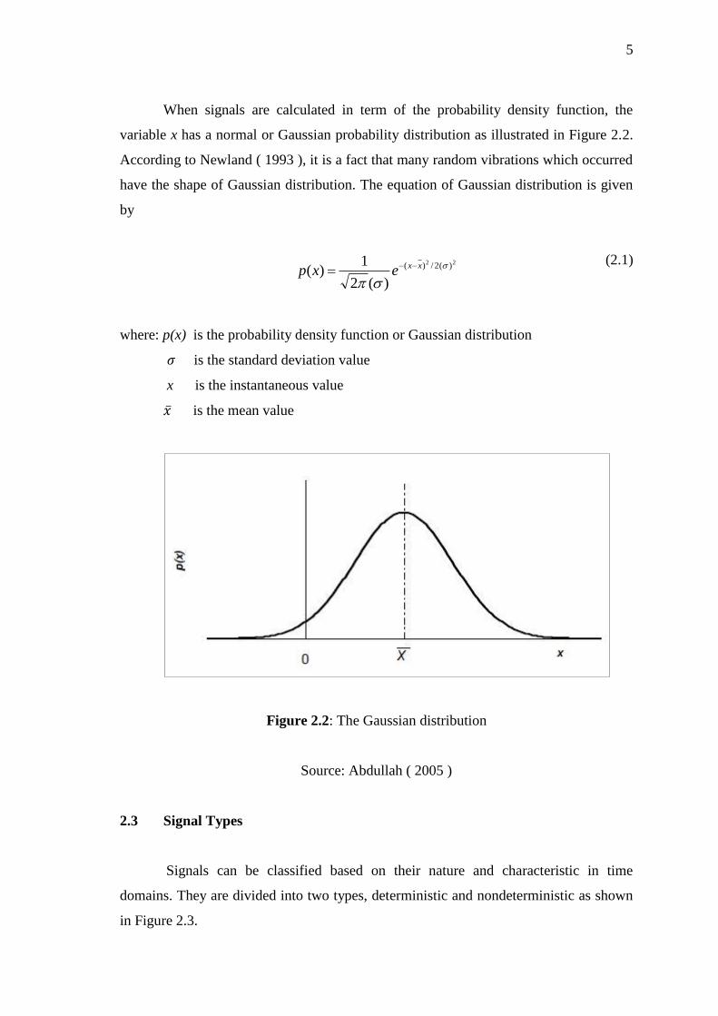
When signals are calculated in term of the probability density function, the

variable x has a normal or Gaussian probability distribution as illustrated in Figure 2.2.

According to Newland ( 1993 ), it is a fact that many random vibrations which occurred

have the shape of Gaussian distribution. The equation of Gaussian distribution is given

by

(2.1)

where: p(x) is the probability density function or Gaussian distribution

is the standard deviation value

x is the instantaneous value

is the mean value

Figure 2.2: The Gaussian distribution


2.3 Signal Types

Signals can be classified based on their nature and characteristic in time

domains. They are divided into two types, deterministic and nondeterministic as shown

in Figure 2.3.

22 )(2/)(

)(2

1)(

xxexp

6

Deterministic signals also known as stationary signals. The signals have the

constant frequency and level content over a long period of time. It also exhibits

statistical properties which remain unchanged with t changes in time. It can further

divisible into periodic and nonperiodic signals. Periodic signals have the pattern of

wavelets which repeat at equal increment of times. It can be categorized into sinusoidal

and complex periodic signals. Nonperiodic signal has the waveform which varies over

the duration of time. It is further divided into almost-periodic and transient.

Sinusoidal signal is represented mathematically by

tfXtx o2sin)( (2.2)

where: X is the amplitude

f o

is the cyclic frequency

x(t) is the instantaneous value at time t

Complex periodic signal is the sum of the amplitudes of its component signal for each

value of the independent variable. These amplitudes are related to the frequency and

phase of the signal. The equation is presented by

(2.3)

n=1,2,3,…

where: f n is the cyclic frequency

n is the phase angles

Almost periodic signal is similar to the complex periodic signal but it contains the sine

wave of arbitrary equations which frequency ratios are not rational number. In other

words, the frequency of one or more of the higher frequency components of the signal is

not an integral multiple frequency of the signal’s lowest frequency component.

Transient signal is defined as nonperiodic signal with a finite time range. ( Bendat and

Piersol, 1986 ) Transient signal includes all other deterministic data which can be

)2sin()(1

nn

n

n tfXtx

7

described by a suitable function. This signal can be described by a step or ramp function.

It occurs at a short period of time and then disappears. Transient signals can be square

pulse, triangular pulse and sine pulse which decay to zero.

Nondeterministic signals are also defined as random signals. Most signals in

nature exhibit the nondeterministic characteristic. A nondeterministic signal is occurred

randomly and the wavelet is irregular. It can further be classified into two categories,

stationary and nonstationary. Stationary signal is the relevant statistical parameters

remain unchanged for the whole signal length. Stationary signal can be divided into two

categories, ergodic and nonergodic. When one sample record of signals is completely

representative of the entire process, the process is ergodic. The mean value and the

autocorrelation do not differ. The mean value x (k) is mathematically defined as

x

T

k dttxT

Tk0

)(1

)lim()( (2.4)

and the autocorrelation function is

R

T

kkx dttxtxT

Tk0

)()(1

)lim(),( (2.5)

where: is the time displacement

T is the period

k is the number of sample function

Nonstationary signal is ones who amplitude and frequency vary with times. It can

divided into mildly nonstationary and heavily nonstationary. According to Priestley

( 1988 ), mildly nonstationary signal is a random process with stable mean, variance and

root mean square value for most of the record, but with short periods of changed signal

statistic due to the present of transient behaviour. Heavily nonstationary signal is

defined in a similar manner to mildly nonstationary signals but it is characterised by the

presence of more transient events. ( Giacamin, et. al., 2000 )

8

Figure 2.3: Typical signal classification


2.4 Signal Statistical Parameter

Statistical parameters are used to classify the random signals. The most

commonly used are the mean value, the standard deviation value, the root-mean-square

( r.m.s.) value, the Kurtosis and the Skewness. The simplest statistic to compute is the

mean value. For a signal with a number of n data points, the mean value is given by

(2.6)

The standard deviation ( SD ) value is measuring the spread of data about the mean

value. The standard deviation is defined as

(2.7)

n

j

jxn

x1

1

2

1

2

1

})(1

{

n

jj

xn

SD x

9

for the samples more than 30. When the samples less than 30, the standard deviation is

mathematically defined as

(2.8)

The root mean square ( r.m.s) value is used to quantify the overall energy content of the

signal and is defined by the following equation:

n

jjx

nsmr

1

2

12}

1{... (2.9)

Kurtosis is a global signal statistic which is the 4th signal statistical moment. It is

highly sensitive to the spikeness of the data. It compares the distribution of the data with

a Gaussian type distribution. The Kurtosis equation is defined as :

K=

n

j

jxsmrn 1

4(

)..(

1x 4) (2.10)

The statistic index Kurtosis represents an indicator for the analysis of damage in low

speed machineries with no continuous shock. It must be used with the global value rms

and time signals. According to Lorenzo and Calabro ( 2007 ), signal with Gaussian data

distribution, for example the acceleration, has the Kurtosis value = 3, while in presence

of impulsive phenomenon, the distribution of data isn’t show the Gaussian shape and

the Kurtosis value is more than 3 due to high amplitude fatigue cycles. Nopiah et al.

( 2009 ) found that, Kurtosis is used for detecting the fault symptons because of the

sensitivity to high amplitude events.

The Skewness, which is the signal 3rd statistical moment. It is a measure of the degree

of symmetry of the distribution of the data points about the mean value. For a Gaussian

random signal, the Skewness is zero value. Positive skewness value is the probability

distributions which are skewed to the right whereas the negative skewness value

2

1

1

2}

1

1{

n

jjx

nSD

10

indicates that the probability distributions which are skewed to the left with respect to

the mean value. The Skewness of a signal is defined as

n

jj

xSDn

S x1

3

3)(

)(

1 (2.11)

2.5 Frequency Domain Analysis

2.5.1 Fourier Transform

Fourier transform is used in signal analysis, quantum mechanics and etc. It is

used to identify the frequency components from a continuous waveform. For signal

processing, Fourier transform is a tool used to transform a time data series domain into

the frequency domain. It is used to convert the non-periodic function of time into a

continuous function of frequency. The Fourier transform pair for continuous signals are

mathematically defined as followed

dtetfF ti

)()(

(2.12)

deFtf ti)(2

1)(

(2.13)

where: F(ω) is the Fourier Transform of f(t)

f(t) is the inverse Fourier transform

ω is the angular frequency

1i

11

2.5.2 Discrete Fourier Transform

Discrete Fourier Transform ( DFT ) is defined as the signal which digitalized by

digital equipment. The signal will become the finite and discrete form of Fourier

Transform. It works well under the condition where a sampled time domain signal

which is periodic. The signal is periodic and decomposed into the sinusoidal form. The

DFT equation is defined as followed

1

0

/21 N

t

Nikt

jke

NxX

(2.14)

where: j, k =0,1,2,3..., ( N-1 )

N is number of sample points in the DFT data frame.

The inverse of the DFT is defined as

1

0

/2N

k

Nijk

kj ex X (2.15)

where: k = 0,1,2,3,..., ( N-1 )

Fast Fourier Transform ( FFT ) is the decomposition of the DFT, which the number of

computations needed for N points from 2N 2 is reduced to 2NlgN. According to Bendat

and Piesol ( 1986 ), power spectral density ( PSD ) is a useful representation of random

signals. PSD describes the general frequency composition of the data in terms of the

spectral density of its mean square values. It has the signal energy which measured

within a certain frequency band.

2.5.3 Short-Time Fourier Transform

Short-Time Fourier Transform ( STFT ) is a method of time-frequency analysis.

It produces information which has a localisation in time. STFT is used for analyzing

non-stationary signals where the statistic characteristic varies with time. By using

12

Fourier analysis, it is not possible to get the frequency information at a particular point

because the Fourier transform is used for analyze the entire signal. STFT extracts

several frames of the signal to be analyzed with a window of signal which moves with

time. Each of the frames can be assumed as stationary for the purpose of analyse. As

Patsias ( 2000 ) pointed out that the Fourier Transform will then be applied to each of

the frame using a window function with the condition that it is typically nonzero at the

analysed segment whereas zero at the outside. In short, for wide analysis window, it will

provide excellent frequency information but poor time resolution. In contrary, for the

narrow analysis window will provide good time resolution but poor frequency

information.

2.6 Total Fatigue Damage

Fatigue is the process responsible for premature failure and damage of the

components which subjected to the repeated loading. ( Bannantine et. al., 1990 ). If the

number of load cycles to failure is less than 1000 cycles, the fatigue is considered as

low cycle. In contrast, when the number of load cycles to failure is more than 1000

cycles, the fatigue is considered as high cycle. Fatigue life analysis is performed at the

early stage of design to reduce the development time and cost. ( Rahman et. al., 2007 )

Three basic approaches have been used to analyze fatigue damage, such as

stress-life approach ( S-N ), strain-life approach ( -N ) and linear elastic fracture

mechanics ( LEFM ). S-N approach is first formulated in the 1850s to 1870s. It used

nominal stress rather than local stress to understand and quantify metal fatigue. The

method does not functionally well in low cycle application. As Rahman et al. ( 2010 )

points out that most components may appear to be subjected to the nominally cyclic

elastic stresses. The stress concentration may present in the component and causes the

load cyclic plastic deformation. However, this approach is suitable to predict high cycle

fatigue and situations in which only elastic stresses and strains are present.

Linear elastic fractured mechanics ( LEFM ) is developed in 1920 but the first

experimental research is done in 1961. It is an analytical method which relates the stress

at the crack tip to the nominal stress field around the crack. LEFM first assumes that the

i a study of the strain signals behaviour ng jun …umpir.ump.edu.my/8431/1/cd8118_@_51.pdf ·...

Documents