hyperspectral image classification using support vector ... · the implementation of hyperspectral...

(IJACSA) International Journal of Advanced Computer Science and Applications,

Vol. 10, No. 10, 2019

271 | P a g e

www.ijacsa.thesai.org

Hyperspectral Image Classification using Support

Vector Machine with Guided Image Filter

Shambulinga M1, G. Sadashivappa

2

Dept of Telecommunication Engineering, RV College of Engineering, Bengaluru

Abstract—Hyperspectral images are used to identify and

detect the objects on the earth’s surface. Classifying of these

hyperspectral images is becoming a difficult task, due to more

number of spectral bands. These high dimensionality problems

are addressed using feature reduction and extraction techniques.

However, there are many challenges involved in the classification

of data with accuracy and computational time. Hence in this

paper, a method has been proposed for hyperspectral image

classification based on support vector machine (SVM) along with

guided image filter and principal component analysis (PCA). In

this work, PCA is used for the extraction and reduction of

spectral features in hyperspectral data. These extracted spectral

features are classified using SVM like vegetation fields, building,

etc., with different kernels. The experimental results show that

SVM with Radial Basis Functions (RBF) kernel will give better

classification accuracy compared to other kernels. Moreover,

classification accuracy is further improved with a guided image

filter by incorporating spatial features.

Keywords—Support Vector Machine (SVM); hyperspectral

images; guided image filter; Principal Component Analysis (PCA)

I. INTRODUCTION

Remote Sensing is the study of collecting the earth’s surface data and information by measuring the reflected signal form objects at long distances. The data collected in the form of images are classified and identified for different objects on the earth’s surface. The major applications of remote sensing are urban planning and management, forestry, environmental monitoring, agriculture, Highway, Resource monitoring, and flood management. Remote sensing techniques are divided into two types, namely infrared and optical remote sensing. In optical remote sensing, an optical sensor in the satellite is used to detect targets by measuring the reflected or scattered solar radiated signal from the earth objects. In infrared remote sensing, the infrared sensor in the satellite is utilized to identify the infrared radiated signal emitted from the earth’s surface.

Optical remote sensing satellite makes use of electromagnetic waves sensor of different wavelength ranging from visible to infrared region in forming images. Solar radiation from the earth surface reflects and absorb at different wavelength band for different materials to form a spectral signature of targets. Depending upon the number of spectral bands utilized in an imaging system, satellite images are classified into three types, panchromatic image, multispectral image, and hyperspectral image. The panchromatic imaging system has a single spectral band with a broad wavelength. Multispectral imaging has few spectral bands contains both brightness and color information of the targets. The hyperspectral imaging system captures the image in more than

100 spectral bands. This hyperspectral image contains the exact spectral information which has better characterization and detection of the objects in the image.

The problems in the classification of hyperspectral images are high dimension which results in the Hughes phenomenon [1]. In the Hughes phenomenon, the accuracy of the supervised classification method decreases as the data dimensionality increases, with fixed training samples and labels. High dimensionality problem in the classification of a hyperspectral image can be overcome by feature selection and extraction techniques. The researchers have developed various feature extraction techniques, for example, Principal component analysis (PCA) [2], Independent component analysis (ICA) [3], and linear discriminant analysis (LDA) [4].

PCA and ICA are unsupervised methods do not require labels and LDA is the supervised method requires labels for extraction of a feature vector. These feature extraction techniques preserve the spectral signature information of different class by projecting a feature vector with more dimension vector to less dimension vector. Among these feature extraction methods, the PCA method will preserve most of the spectral information of a hyperspectral image in a small amount of principal components. The feature selection technique tries to find out the best spectral bands in hyperspectral images to achieve the highest class separability. Different types of methods developed based on distance and information theory [5] for the spectral band selection in hyperspectral images. Experimental results of these feature selection methods have shown better performances, but these methods have some theoretical difficult in finding the best subset combination of features for classification.

More number of pixel-wise classifiers was proposed for the classification and identifying targets in a hyperspectral data such as random forests [6], neural networks [7], Adaboost, SVM with various kernels, sparse representation [9] and active learning [10]. SVM is the better pixel-wise classifier compare to other classifiers and also shown better performance in terms of the overall accuracy of classification. SVM requires less number of training samples and labels to obtain good classification accuracy and it is also robust to spectral dimensions in hyperspectral images. Furthermore, many researchers have tried to enhance the performance of the classification by considering the spectral and spatial feature classification techniques [11], which includes spatial information to the pixel-wise classifier. Some image fusion techniques [12] are utilized to enhance the spectral and spatial information.


Vol. 10, No. 10, 2019

272 | P a g e


In addition to spatial feature extraction, another spectral and spatial classification method has been developed based on image segmentation [13]. In this, segmentation of the hyperspectral image is performed based on similarity and homogeneity of spectral information, so that all pixels in the region are considered as the same class. Various segmentation techniques have been developed for hyperspectral images such as watershed [15], partitional clustering [14], minimum spanning forest [17] and hierarchical segmentation [16]. However, the classification of these methods depends on the performance of the segmentation. Most of the advanced segmentation algorithms are time-consuming.

Recently, a guided image filter [18] is used as edge-preserving filter for most of the applications such as enhancing and denoising the images and high dynamic imaging. This guided image filter can be used to enhance the SVM classification accuracy [8] of the hyperspectral images by considering spatial features.

Hyperspectral image classification based on SVM with a guided image filter and PCA is proposed in this paper. Here PCA is used as a dimensionality reduction algorithm for reducing the feature vectors and also the first principal component of spectral features are used as a guidance image for guided image filter.

This paper is organized as follows: Section II introduces the theory of PCA for feature reduction. Section III gives the basic idea of SVM with different kernels for classification. Section IV describes the theory of guided image filter to improve the performance of classification. Section V describes the methodology of hyperspectral classification. Section VI and VII discusses the experimental results of hyperspectral classification and conclusion.

II. PRINCIPAL COMPONENT ANALYSIS

PCA is the dimensionality reduction algorithm for the hyperspectral images in which bands are highly correlated and convey similar information. The original data bands are analyzed and transformed to remove the correlation in the bands. Statistics properties are used in PCA to remove the correlated bands. The basic principle used in PCA is the eigenvalue decomposition of the covariance matrix. The detailed steps of PCA for a hyperspectral image are as follows.

Consider the hyperspectral image has N bands. Each pixel of the image is defined by a vector

[ ] (1)

where x1, x2, x3…..xN are the data number of the respective bands. In hyperspectral image has m rows and n columns which leads to a total of M=m*n such vectors. The mean value for each vector defined in (1) is calculated by using (2).

∑ [ ]

(2)

The covariance matrix is calculated by using (3)

∑ ( )( )

(3)

PCA is based on the eigenvalue decomposition of the covariance matrix which is given in (4)

(4)

where,

( ) (5)

D is the diagonal matrix contains the eigenvalues of the covariance matrix and A is the orthonormal matrix of N dimension eigenvector ak of CX

( ) (6)

Linear transformation Yi is the PCA pixel vector given by (7)

(7)

Pixel vectors in (7) are PCA bands of the original hyperspectral image.

Let eigenvector and eigenvalues are arranged in descending

order, say, 1 > 2 >3 4>….>N, first K rows of matrix in equation (7) can be used to calculate the approximation of the original images as mentioned in (8)

[

]

[

]

[ ]

(8)

Pixel vector is the first K bands of PCA images. These PCA image has the highest contrast or variance in the first band and lowest contrast or variance in the last band. Thus PCA contains a majority of information in the first few bands of the hyperspectral images.

III. SUPPORT VECTOR MACHINE

SVM is derived based on the decision planes that determine decision boundaries. A decision plane sorts out between a set of objects having various class memberships. SVM classifier separates the data into a training set and testing set. Each instance in the training set is assigned to one target value. Let X be the input data set and Y be the output dataset. Training set be {(x1, y1), (x2, y2), ……. (xm, ym)}. Try to find out the

suitable value of yY from the previously seen value xX. SVM model can be generated by the equation

( ) (9)

here, are the parameters of the kernel function that needs to be fine-tuned for accurate classification. SVM classifier has various types of kernel functions such as polynomial, linear, and radial basis functions. SVM methodology with a linear kernel is shown in Fig. 1. Here, H is the optimal hyperplane and it should have a maximum margin value to separate the two classes. The SVM decision function is given by (10)

( ) ∑ ( ) (10)

( ) is the kernel function and S is training sample

subsets.


Vol. 10, No. 10, 2019

273 | P a g e


Fig. 1. Linear SVM Methodology.

Some of the commonly used kernels are:

Linear:

( ) ⟨ ⟩

Polynomial:

( ) ( ⟨ ⟩ )

Radial basis function:

( ) { ‖ ‖

}

Sigmoid:

( ) ( ⟨ ⟩ )

IV. GUIDED IMAGE FILTER

Guided Image filter is an Edge preserving filter that defines a linear translations variant filtering process, contains guidance image and input image . Depending on the application, guidance image can be same as the input or any other image. Guided image filter output as defined in (11) is a linear transform of a guided image in a window of particular size centered at pixel k

(11)

and are the linear coefficients determined by minimizing cost function between the filter output q and filter input p

( ) ∑ (( )

) (12)

is the regularization parameter and solution to equation (12) is given by linear regression

| |∑

(13)

(14)

here, is the mean and is the variance of in , | |

is the total number of pixel in .

Apply a linear model to every local window in an image and filter output is computed by equation (15).

| |∑ ( )

(15)

Where

| |∑

and

| |∑

V. METHODOLOGY

The implementation of hyperspectral image classification using the SVM classifier technique is shown in Fig. 2. In the implementation, a hyperspectral image data with 224 spectral bands of different wavelengths are considered. The estimated size of the image data is three dimensional because the image is captured at different wavelengths. Convert the three-dimensional data to two-dimensional data for SVM classification. Since the spectral information in the image data contains more dimensions which consume more time for classification, so the dimensions of the data are reduced using PCA as shown in Fig. 3. The supervised classification requires training samples and training labels. In the given set of data samples, randomly select and normalize the training samples and testing samples with labels associated to the respective sample.

Fig. 2. Flow Chart of Hyperspectral Image Classification.

Kernel based learning approach for satellite image

classification using support vector machine

S.Manthira Moorthi, Indranil Misra, Rajdeep Kaur, Nikunj P Darji and R. Ramakrishnan Data Products Software Group, Signal and Image Processing Area

Space Applications Centre (ISRO)

Ahmedabad 380015, India

E-Mail: {smmoorthi, indranil, rajdeep,nikunj,rama}@sac.isro.gov.in

Abstract--Machine learning is a scientific computing discipline to

automatically learn to recognize complex patterns and make

intelligent decisions based on the set of observed examples

(training data). Support Vector Machine (SVM) is a supervised

machine learning method used for classification. An SVM kernel

based algorithm builds a model for transforming a low dimension

feature space into high dimension feature space to find the

maximum margin between the classes. In the field of geospatial

data processing, there is a high degree of interest to find an

optimal image classifier technique. Many image classification

methods such as maximum likelihood, K-Nearest are being used

for determining crop patterns, land use and mining other useful

geospatial information. But SVM is now considered to be one of

the powerful kernel based classifier that can be adopted for

resolving classification problems. The objective of the study is to

use SVM technique for classifying multi spectral satellite image

dataset and compare the overall accuracy with the conventional

image classification method. LISS-3 and AWIFS sensors data

from Resourcesat-1, Indian Remote Sensing (IRS) platform were

used for this analysis. In this study, some of the open source tools

were used to find out whether SVM can be a potential

classification technique for high performance satellite image

classification.

Keywords-- Support Vector Machine; IRS; geospatial

information; image classification; maximum likelihood classifier;

SVM classification

I. INTRODUCTION

The satellite image classification is a mechanism to group

together pixels that have similar radiance/digital number value

across a series of image bands or information channels. This

extraction of information from remote sensing data is now

driven by using various statistical learning methods. SVM is

one of the kernel based machine learning algorithm. SVM

learning theory is developed for solving pattern recognition

problem, to build classification and regression techniques in

diverse technological fields including remote sensing

discipline [3]. SVM is based on the concepts of decision

surface. A decision surface separates the classes in such a way

that maximizes the margin between the classes. This surface is

also known as optimal hyper plane. The data points close to

the optimal hyper plane are called support vectors. The

support vectors are critical elements in training sample set

creation [6].

II. PRINCIPLE OF SVM

The principle of SVM classification is to separate the data

into training set and testing/prediction set. Each instance in the

training set contains one target value and several attributes

which can be features and predictor variables [7].

Let X and Y be the input and output datasets and the

training set be {(x1, y1), (x2, y2)……….. (xm, ym)}. In general,

according to a previously seen value Xx Î , we try to find a

suitable Yy Î .So we try to learn a classifier or generate a

SVM model by:

α)f(x,Y = (1)

where α are the parameters of the kernel function that need to

be fine tuned for more accurate image classification results.

The SVM Classifier can do the learning with different types of

kernel functions such as linear, polynomial and radial basis

function for effective image classification [1]. SVM

methodology is depicted in Fig. 1.

Fig. 1 Linear SVM Methodology

All hyper planes are parameterized by a normal vector w

which is perpendicular to the hyper plane and a constant b. It

can be expressed as

f(x) = w.x + b (2)

H is the optimal hyper plane which can be expressed as

H: xi.w + b = 0 (3)

d+

Optimal

Hyper plane

H

H1

-1

+1

H2

w.x+b=0

w.x+b=+1

w.x+b=-1

Support Vectors

d-

978-1-4244-9477-4/11/$26.00 ©2011 IEEE

107


Vol. 10, No. 10, 2019

274 | P a g e


Fig. 3. Flow Chart of PCA Implementation.

Fig. 4. Flow Chart of n-fold Cross Validation.

Fig. 5. Flow Chart of Guided Image Filter Implementation.

Using training samples SVM model is developed with a different kernels. Cost function and gamma parameter for RBF kernel are calculated using the n-fold cross-validation approach as shown in Fig. 4. This approach tries to find the best cost function and gamma parameter which has the highest training accuracy. The developed SVM model with different kernel parameters is utilized to predict the different classes of various test samples of the hyperspectral dataset. Evaluate the performance of the model by computing a confusion matrix to find the classification accuracy and computational time. Guided image filter, as shown in Fig. 5, is used to improve the

training accuracy by averaging the misclassified data with nearby classified data using regularization parameters and the first component of PCA as a guidance image.

VI. EXPERIMENTAL RESULTS AND DISCUSSIONS

A. Experimental Setup

Hyperspectral Data Sets: The Indian pines image dataset has been used to analyze the performance of the proposed approach. This hyperspectral dataset captured through the Airborne Visible/ Infrared Imaging Spectrometer (AVIRIS) sensor at the Indian test site of North-Western Indiana. These data sets contain the spectral information of 220 bands with a

spectral wavelength of 0.4 to 2.5m of size 145 x 145 pixels.

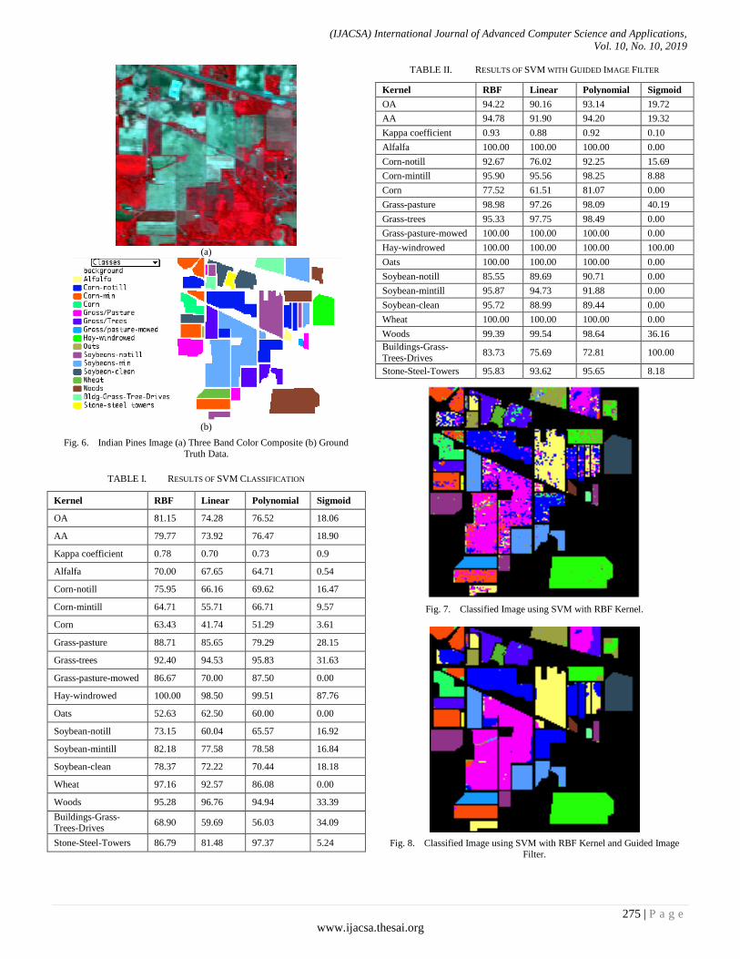
The spatial resolution of the Indian pines dataset is 20 m per pixel. The image dataset has 16 classes of different agriculture, vegetation, and forest information. The number of spectral bands in an image dataset is reduced to 200 by removing unnecessary spectral band covered with the water absorption region. The Three band color composite and its ground truth data of various classes of the Indian Pines image are shown in Fig. 6.

Performance parameters: The performance parameters used to analyze the performance of the proposed classification method are overall accuracy (OA), the average accuracy (AA), and the Kappa coefficient. OA is the ratio of a number of pixel samples classified to accurate class to the total number of pixel samples in the dataset. AA is the mean classification accuracy of various classes that is present in the dataset. The Kappa coefficient is a performance parameter of classification that gives the percentage of data samples classified accurately to the respective classes of a hyperspectral dataset, corrected by the number of arguments.

B. Classification Results

Indian Pines image dataset is classified using SVM with different kernels and guided image filter by considering the 10% of training samples of various classes. The results of the SVM classification accuracy of different kernels and guided image filter are shown in Table I and Table II, respectively.

The results infers that the SVM classifier with RBF kernel has the highest overall classification accuracy of 81.15 %. The classified image of different vegetation fields is shown in Fig. 7. Guided image filter is used after SVM classification to improve the overall accuracy from 81.15 to 94.22 % for RBF kernel. The classified image of different vegetation fields with a guided image filter is shown in Fig. 8. The computation time required for the complete process is 155 seconds.

The computation time required for the SVM is reduced by considering the PCA and removing the unnecessary spectral information of the hyperspectral image. These reduced principal components are used as a feature vector to classify the image using SVM and Guided image filter. Fig. 9 and 10 demonstrate SVM classification accuracy and computational time required for classification with respect to the number of principal components. Fig. 9 shows that SVM with 20 principal components will give the classification accuracy of 79 % with a computation time of 38 seconds. Classification accuracy is improved to 89 % after using the guided image filter.


Vol. 10, No. 10, 2019

275 | P a g e


(a)

(b)

Fig. 6. Indian Pines Image (a) Three Band Color Composite (b) Ground

Truth Data.

TABLE I. RESULTS OF SVM CLASSIFICATION

Kernel RBF Linear Polynomial Sigmoid

OA 81.15 74.28 76.52 18.06

AA 79.77 73.92 76.47 18.90

Kappa coefficient 0.78 0.70 0.73 0.9

Alfalfa 70.00 67.65 64.71 0.54

Corn-notill 75.95 66.16 69.62 16.47

Corn-mintill 64.71 55.71 66.71 9.57

Corn 63.43 41.74 51.29 3.61

Grass-pasture 88.71 85.65 79.29 28.15

Grass-trees 92.40 94.53 95.83 31.63

Grass-pasture-mowed 86.67 70.00 87.50 0.00

Hay-windrowed 100.00 98.50 99.51 87.76

Oats 52.63 62.50 60.00 0.00

Soybean-notill 73.15 60.04 65.57 16.92

Soybean-mintill 82.18 77.58 78.58 16.84

Soybean-clean 78.37 72.22 70.44 18.18

Wheat 97.16 92.57 86.08 0.00

Woods 95.28 96.76 94.94 33.39

Buildings-Grass-Trees-Drives

68.90 59.69 56.03 34.09

Stone-Steel-Towers 86.79 81.48 97.37 5.24

TABLE II. RESULTS OF SVM WITH GUIDED IMAGE FILTER

Kernel RBF Linear Polynomial Sigmoid

OA 94.22 90.16 93.14 19.72

AA 94.78 91.90 94.20 19.32

Kappa coefficient 0.93 0.88 0.92 0.10

Alfalfa 100.00 100.00 100.00 0.00

Corn-notill 92.67 76.02 92.25 15.69

Corn-mintill 95.90 95.56 98.25 8.88

Corn 77.52 61.51 81.07 0.00

Grass-pasture 98.98 97.26 98.09 40.19

Grass-trees 95.33 97.75 98.49 0.00

Grass-pasture-mowed 100.00 100.00 100.00 0.00

Hay-windrowed 100.00 100.00 100.00 100.00

Oats 100.00 100.00 100.00 0.00

Soybean-notill 85.55 89.69 90.71 0.00

Soybean-mintill 95.87 94.73 91.88 0.00

Soybean-clean 95.72 88.99 89.44 0.00

Wheat 100.00 100.00 100.00 0.00

Woods 99.39 99.54 98.64 36.16

Buildings-Grass-

Trees-Drives 83.73 75.69 72.81 100.00

Stone-Steel-Towers 95.83 93.62 95.65 8.18

Fig. 7. Classified Image using SVM with RBF Kernel.

Fig. 8. Classified Image using SVM with RBF Kernel and Guided Image

Filter.


Vol. 10, No. 10, 2019

276 | P a g e


Fig. 9. Variation of OA in SVM with Number of Principal Components.

Fig. 10. Variation of Computation Time with Respect to Number of Principal

Components Considred in SVM.

VII. CONCLUSIONS

In this paper, a spectral and spatial classification method was developed for the hyperspectral image classification. The proposed approach uses the SVM classifier with kernels for the classification. The results shows that the RBF kernel will have the highest overall accuracy. Hyperspectral image contains many numbers of bands so more computational time is required to compute the kernel parameters and classification maps. In order to minimize the computational time, spectral features are reduced using PCA and only a few principal components are used for the classification. Furthermore, the classification accuracy of the SVM is increased by using the guided image filter with the first principal component has a guided image. From the experimental results it can be inferred that overall accuracy is improved from 81.15% of SVM to 94.22% for RBF kernel with the same training samples. In the future scope, computational time of the classification can be further reduces by employing supervised dimensionally reduction algorithm.

REFERENCES

[1] G. Hughes, “On the mean accuracy of statistical pattern recognizers,” IEEE Transactions Information Theory, vol. IT-14(1), pp. 55–63, 1968.

[2] S. Prasad and L. M. Bruce, “Limitations of principal components analysis for hyperspectral target recognition,” IEEE Geoscience Remote Sensing Letter., vol. 5( 4), pp. 625–629, 2008.

[3] A. Villa, J. A. Benediktsson, J. Chanussot, and C. Jutten, “Hyperspectral image classification with independent component discriminant analysis,” IEEE Transactions Geoscience Remote Sensing, vol. 49(12), pp. 4865–4876, 2011.

[4] W. Li, S. Prasad, J. E. Fowler, and L. M. Bruce, “Locality-preserving dimensionality reduction and classification for hyperspectral image analysis,” IEEE Transactions Geoscience Remote Sensing., vol. 50(4), pp. 1185–1198, 2012.

[5] B. Guo, S. R. Gunn, R. I. Damper, and J. D. B. Nelson, “Band selection for hyperspectral image classification using mutual information,” IEEE Geoscience Remote Sensing Letters., vol. 3(4), pp. 522–526, 2006.

[6] M. Dalponte, H. O. Orka, T. Gobakken, D. Gianelle, and E. Nasset, “Tree species classification in boreal forests with hyperspectral data,” IEEE Transactions Geoscience Remote Sensing, vol. 51(5), pp. 2632–2645, 2013.

[7] Y. Zhong and L. Zhang, “An adaptive artificial immune network for supervised classification of multi-/hyperspectral remote sensing imagery,” IEEE Transactions Geoscience Remote Sensing, vol. 50(3), pp. 894–909, 2012.

[8] T. Dundar and T. Ince, "Sparse Representation-Based Hyperspectral Image Classification Using Multiscale Superpixels and Guided Filter," in IEEE Geoscience and Remote Sensing Letters, vol. 16(2), pp. 246-250, 2019.

[9] Y. Chen, N. M. Nasrabadi, and T. Tran, “Hyperspectral image classification via kernel sparse representation,” IEEE Transactions Geoscience Remote Sensing., vol. 51(1), pp. 217–231, Jan. 2013.

[10] J. Li, J. M. Bioucas-Dias, and A. Plaza, “Spectral–spatial classification of hyperspectral data using loopy belief propagation and active learning,” IEEE Transactions Geoscience Remote Sensing., vol. 51(2), pp. 844–856, Feb. 2013.

[11] A. Mughees and L. Tao, "Multiple deep-belief-network-based spectral-spatial classification of hyperspectral images," in Tsinghua Science and Technology, vol. 24(2), pp. 183-194, 2019.

[12] K. Suchitha, B.S. Premananda and A.K. Singh, "High spatial resolution hyperspectral image using fusion technique," International Conference on Trends in Electronics and Informatics, pp. 348-353, 2017.

[13] A. Datta and A. Chakravorty, "Hyperspectral Image Segmentation using Multi-dimensional Histogram over Principal Component Images," International Conference on Advances in Computing, Communication Control and Networking, pp. 857-862, 2018.

[14] Y. Tarabalka, J. A. Benediktsson, and J. Chanussot, “Spectral–spatial classification of hyperspectral imagery based on partitional clustering techniques,” IEEE Transactions Geoscience Remote Sensing., vol. 47(8), pp. 2973– 2987, 2009.

[15] R. Gaetano, G. Masi, G. Poggi, L. Verdoliva and G. Scarpa, "Marker-Controlled Watershed-Based Segmentation of Multiresolution Remote Sensing Images," in IEEE Transactions on Geoscience and Remote Sensing, vol. 53(6), pp. 2987-3004, 2015.

[16] A. M. Braga, R. C. P. Marques, F. A. A. Rodrigues and F. N. S. Medeiros, "A Median Regularized Level Set for Hierarchical Segmentation of SAR Images," in IEEE Geoscience and Remote Sensing Letters, vol. 14(7), pp. 1171-1175, 2017.

[17] F. Poorahangaryan and H. Ghassemian, "Spectral-spatial hyperspectral classification with spatial filtering and minimum spanning forest," 9th Iranian Conference on Machine Vision and Image Processing, pp. 49-52 2015.

[18] X. Kang, S. Li, and J. A. Benediktsson, “Spectral–spatial hyperspectral image classification with edge-preserving filtering,” IEEE Transactions Geoscience Remote Sensing., vol. 52(5), pp. 2666–2677, 2014.

40

50

60

70

80

90

10010

20

30

40

50

60

70

80

90

10

0

11

0

12

0

13

0

14

0

15

0

16

0

17

0

18

0

19

0

20

0

Overa

ll A

ccu

ra

cy

(%

)

Number of Principal Components

SVM classificaiton with PCA Decompostion

SVM SVM_GIF

0

20

40

60

80

100

120

140

160

180

200

10

20

30

40

50

60

70

80

90

10

0

11

0

12

0

13

0

14

0

15

0

16

0

17

0

18

0

19

0

20

0

Tim

e (

seco

nd

s)

Number of Principal Components

Computation time (seconds)

hyperspectral image classification using support vector ... · the implementation of hyperspectral...

Documents