hydrological and agro-ecological data acquisition using remotely...

Agrifood Research Reports 68, p. 159-177.

159

______________________ MTT Agrifood Research Finland

Hydrological and Agro-ecological Data Acquisition using Remotely Sensed Data from

Satellite Sensors

Sevket Durucan, Dimitrios Papanastasopoulos and Anna Korre.

Environmental Processes and Systems Research Group, Department of Environmental Science and Technology, Imperial College London, London SW7 2AZ, United Kingdom, [email protected]

Abstract Research at Imperial College developed a methodology to extract time-space dependent hydrological parameters form Remote Sensing data in order to predict land surface temperature from satellite observations. Time series of actual ET were estimated using both the SVAT model and the water balance model. The comparison of cumulative ET between the two different methods shows a good agreement and validates the developed parameterisation. Plant growth as it is described by the temporal signal of SAR data and interpreted by the optical data for the presence and status of vegetation in a distributed manner over the entire area, is proven to be very close to the traditionally reliable method of estimating losses using a hydrologic engineering model calibrated against hourly river flow data. The cumbersome process of select-ing parameters for every discredited modelling unit has been replaced by a simple automated procedure after converting the SAR temporal signal into a dimensionless growth factor. Different runs of the system of SVAT columns employing different functions linking the derived growth factor and bio-physical parameters, as well as, different sets of maximum and minimum values for the time dependent plant growth parameters were used.

Key words: hydrology, agro-ecology, Remote Sensing


160

1. Introduction

In a natural hydrologic system much of the water that falls as precipitation returns to the atmosphere through evaporation from vegetation, bare soil sur-faces, water bodies, and through transpiration from vegetation. In estimating the losses of the system through evaporation and transpiration the detailed physics of heat and water transfer between the soil and the atmosphere must be accounted for. A special emphasis is put on land surface, because this is the interface of the exchange of mass and energy fluxes. Evapotranspiration, the combined evaporation and transpiration, is the process that extracts both moisture and energy from land’s surface. It accounts for a large percentage of the total water balance, and it is strongly variable over both space and time.

Remote sensing has held a great deal of promise for hydrology, mainly be-cause of the potential to observe areas and entire river basins rather than merely points. Its global coverage can provide the necessary information for use in hydrological models to assess water resources. However the different parts of the electromagnetic spectrum reflected or emitted by the Earth’s sur-face measured by satellite sensors are generally not directly related to the required inputs or outputs for any particular model. Therefore, intermediate models or algorithms are required to interpret the remotely sensed data.

Soil-Vegetation-Atmosphere Transfer (SVAT) models used to simulate the energy and mass exchange in a coupled heat and moisture model require data which are time and space dependent. These parameters include temperature, moisture content, plant height, effective rooting depth, leaf area index, char-acteristic leaf dimension, dry plant biomass, soil types and hydraulic proper-ties, surface roughness and depression storage. Scarcity and sparseness of ground observations regarding these parameters and variables, as well as, accuracy and uncertainty of any indirect methods and instruments used for their estimation makes it an important research problem that needs to be ad-dressed and resolved.

This paper reports on research which aimed at:

Developing a methodology to extract time-space dependent parame-ters form Remote Sensing data,

Developing a technique to assimilate satellite observations in the Temperature-Vegetation index space in models.

Assessing the potential of estimating surface moisture using satellite surface temperature measurements and energy balance models through model inversion, and

Predicting land surface temperature and compare with satellite ob-servations.


161

2. Field site and data used

The area studied in this research includes sub-catchments of the rivers Bor-row, Nore, Boro, Urrin and Slaney, in South- South East Ireland (Figure 1). The climate is temperate, affected by the North Atlantic Current; experienc-ing mild winters, cool summers, and generally overcast. The type of terrain encountered in the area is of low relief, with moderate roughness, which is suitable for the use of SAR sensors. Land use is basically permanent pastures (68%), however, the main disadvantage is the fact that Ireland is frequently under cloud cover, and that it does not allow for extensive use of optical sen-sors.

Elevation ranges from 15m to 780m, with an average elevation of 112m. The period of analysis is from 1/8/1998 to 30/05/2002, and time series of mete-orological data covering the entire period of study were obtained from Kil-kenny and Birrh, two regional stations operated by the Irish Meteorological Office. Data includes precipitation, air temperature, relative humidity, wind speed, global radiation, and river flow, at an hourly time step.

The area covered by the satellite images (Figures 1a and 1b) includes several sub-catchments. Agricultural fields are clearly visible in the optical image (Figure 2a), which is a combination of three bands (two visible and one near infrared) of the ASTER image. The same area is also shown in the SAR im-age acquired a few days later (Figure 2b).

(a)

(b)

(c)

Fig. 1. a) A 3D view of the area with an ASTER image draped on the digital elevation model (an exaggeration factor for elevation has been applied). b) The ERS satellite footprint.


162

Latitude

(a) (b) ESA®

Fig. 2. a) A smaller area in an ASTER image and b) The same area as in a in the SAR image.

Satellite data were obtained from the Advance Spaceborne Thermal Emission and Reflection Radiometer (ASTER) sensor on board NASA’s Terra plat-form, and the synthetic aperture radar system on board ESA’s second Euro-pean Remote Sensing Satellite (ERS-2). The analysis of ERS SAR using ASTER VNIR and TIR images was based on three dates for the SAR (18/11/2000, 03/03/2001, and 07/04/2001), and another three dates for the ASTER images (21/10/2000, 17/2/2001, and 24/2/2001). All ASTER images fall within the ERS footprint (Figure 3). The ASTER images were used for the calculation of vegetation indices and kinetic temperature.

52.5

53

53.5

54

54.5

-7.5 -7 -6.5 -6 -5.5 -5

2/17/01

2/17/01

2/24/01

10/21/00

10/21/00

Longitude

Fig. 3. Area coverage of ASTER images within the ERS footprint for selected dates (not in scale).

3. Hydrologic processes and the description of the model

The temperature of the air near the surface and the temperature of the surface itself reflect the balance of the various surface energy flux components. Methods used to quantify the components of the water and energy balance equation using remote sensing commonly express the water balance equation as follows:


163

QETPtS −−=

∆∆

where ∆S/∆t is the change in storage in the soil, P is the precipitation, ET is the evapotranspiration and Q is the runoff, and the energy balance at the land surface is represented as:

LEHGRN +=−

where RN is the net radiation, G is the soil heat flux, H is the sensible heat flux and LE is the latent heat flux. RN - G is commonly referred to as the available energy, and ET and LE represent the same water vapour exchange rate across the surface–atmosphere interface, except ET is usually expressed in terms of depth of water over daily or longer time scales.

Two hydrologic models, a water balance model HEC HMS US (Army Corps of Engineers, 2003), and a one dimensional stand-alone SVAT model SHAW (US Department of Agriculture, 2000) were used for the simulations carried out in this work.

Water balances are obtained from the HEC Hydrologic Modelling System using the continuous soil-moisture accounting model SMA (Bennett, 1998). The model simulates the movement of water through vegetation and storage on vegetation, soil surface, in the soil profile, and in the groundwater layers (Figure 4).

Fig. 4. A graphical representation of HEC HMS


164

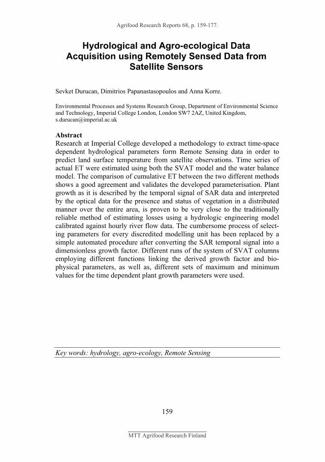
Energy and water transfer model (SVAT) simulates the two state variables and the relationship between the Satellite data and the SVAT model is as shown in Figure 5.

Fig. 5. The relationship between the Satellite data and the SVAT model

3.1 Vegetation indices – Retrieval of Biophysical Properties

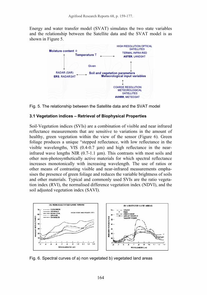
Soil-Vegetation indices (SVIs) are a combination of visible and near infrared reflectance measurements that are sensitive to variations in the amount of healthy, green vegetation within the view of the sensor (Figure 6). Green foliage produces a unique “stepped reflectance, with low reflectance in the visible wavelengths, VIS (0.4-0.7 µm) and high reflectance in the near-infrared wave lengths NIR (0.7-1.1 µm). This contrasts with most soils and other non-photosynthetically active materials for which spectral reflectance increases monotonically with increasing wavelength. The use of ratios or other means of contrasting visible and near-infrared measurements empha-sises the presence of green foliage and reduces the variable brightness of soils and other materials. Typical and commonly used SVIs are the ratio vegeta-tion index (RVI), the normalised difference vegetation index (NDVI), and the soil adjusted vegetation index (SAVI).

Fig. 6. Spectral curves of a) non vegetated b) vegetated land areas


165

NDVI is the most commonly used index for satellite imagery. The difference in reflectances is divided by the sum of the two reflectances. This compen-sates for different amounts of incoming light and produces a number between 0 and 1. The typical range of actual values is about 0.1 for bare soils to 0.9 for dense vegetation. NDVI is thought to be more sensitive to low levels of vegetative cover, while the RVI is more sensitive to variations in dense cano-pies. NDVI is calculated as follows

dNIRdNIRNDVI

ReRe

ρρρρ

+−=

where NIRρ and dReρ are the reflectance at the near infra-red and red channels accordingly.

The radar backscattering coefficient can also provide information about the imaged surface for the discrimination, monitoring, and extraction of bio-physical properties, of agricultural crops with various degrees of success. They rely basically on the comparison of crop biophysical properties with direct measurements on the field, or with the simulated results of models. However, if field measurements are limited or even not possible at all, SAR signatures should be only judged upon results previously obtained with train-ing over optical images, or very limited ground knowledge of land use.

4. Data processing and model simulations

The ERS SAR and TERRA ASTER image products were used for the extrac-tion of hydrologic information for the sub-catchments of the rivers Borrow, Nore, Boro, Urrin and Slaney in Ireland. This information was assimilated in hydrologic models in order to estimate mass and energy fluxes over space.

The HEC HMS model was used to simulate river flow by estimating all the components of the hydrological cycle, including losses to evapotranspiration from measured potential values. An alternative procedure of calculating losses to the atmosphere from water balance estimations is the energy bal-ance estimations using a SVAT model such as SHAW. In SHAW simula-tions, evapotranspiration is explicitly accounted for by the model.

Optical images constitute a very reliable source of information with respect to vegetative cover of the surface in great spatial detail. However, due to the fact that satellite revisit time over the same area is 16 days, and cloud cover usually obstructs the view in northern latitudes, only a few images are usually available within a period of three years. The first available image of the area from the ASTER sensor was in early 2000, and therefore only recently a sat-isfactory number of images, which may provide some statistical inference in the findings, could have been collected. However, if a relationship between vegetation indices and the SAR signal, which can be available on a regular


166

basis, is established, then it is possible to derive the space-time distribution of vegetation properties using the SAR time series and just a small number of optical images.

4.1 Water balance simulations

Several sub-catchments and river segments were defined using the HEC GEOHMS geographical information systems interface for hydrologic pre-processing (Figure 7). This allowed for the extraction of various hydrologic characteristics of river basins from digital elevation models. Each sub-catchment was modelled with a different Soil Moisture Accounting Unit (SMA) allowing for a more suitable selection of parameters based on topog-raphic and land use characteristics of the particular area.

Fig 7. A graphical representation of the hydrologic system

The HEC Hydrologic Modelling System (HEC-HMS) was used to simulate the rainfall-runoff process. The SMA units were represented by a five-layer system with evapotranspiration, which models all losses. Storage volumes and maximum percolation rates between layers were determined by calibra-tion. Rainfall that does not infiltrate, or falls on impervious-saturated areas was routed to the basin outlet using the kinematic wave method. Baseflow was modelled using an exponential decline, a classical separation technique. The reach element routes flow to the outlet using the kinematic wave method. The method attenuates a flood wave by friction and storage as it passes through the reach. Monthly potential evapotranspiration estimates from the local climatic station were provided as input.

HEC HMS model was run for the four-year period 1998-2001 on an hourly basis. The area modelled is a 380 km2 section of river Barrow catchment. The meteorological data recorded at Kilkenny were used to drive the model. Calibration of maximum infiltration rates and storage capacities was per-formed for the first 12 months, and yielded a simulated flow which matched the measured flow with a correlation coefficient R equal to 0.97 and an aver-


167

age residual flow of 3.46 m3/s (Figure 8). For the validation period (second year) the average flow residual was 3.28 m3/s (Figure 9). The length of the channel, the average width of the area drained along the channel length, and the slope characteristics were estimated from the optical image and the digital elevation model.

Fig. 8. Simulated and observed river flow at the exit of the basin.

Fig. 9. Simulated versus observed flow for the validation period.

4.2 SAR data processing and analysis

Synthetic aperture radar data used in this research consists of 10 precision images (PRI) acquired by ERS-2 satellite and supplied to the project by the European Space Agency within the framework of an ESA EO exploitation project. These data are multi-look, ground range, system corrected image data. The backscattering coefficient was calculated using the algorithm of Laur et al. (1996). The resulting backscatter image in dB values were com-pared with the simple vegetation index, as well as with the most common normalised vegetation index and the near infrared reflectance (Figure 10).


168

Strong linear relationship between every vegetation index and the SAR inten-sity in the range 200 to 500, or -7 to -15 for SAR backscatter in dB, have shown that SAR can yield results that are reasonably close to the accuracy of optical images in land surface monitoring, and can be used to form a time series which will satisfactorily track changes of the vegetative surface cover.

In order to identify bare soil fields in the SAR images, a threshold value of 500 was used, and all pixels with a value higher than the threshold were in-cluded in the new image (Figure 11a). The process was repeated for a NDVI image with the threshold selected at 0.20 (Figure 11b). The area identified from SAR is 19.13% of the total image area, whereas for the NDVI this was 17.87%, a very good agreement although the shapes do not compare well.

R2 = 0.8904

0

0.5

1

1.5

2

2.5

3

3.5

4

-15-14-13-12-11-10-9-8-7-6-5-4-3-2

SAR backscatter [dB]

Sim

ple

Veg

etat

ion

Inde

x

R2 = 0.8683

00.10.20.30.40.50.60.70.80.9

1

-15-14-13-12-11-10-9-8-7-6-5-4-3-2


Nor

mal

ised

Veg

etat

ion

Inde

x

R2 = 0.8904

20253035404550556065707580

-15-14-13-12-11-10-9-8-7-6-5-4-3-2


NIR

refle

ctan

ce

Fig. 10. SAR backscatter relation with vegetation indices and NIR reflec-tance.

a) b)

Fig. 11. Segmentation via thresholding for a SAR and an NDVI sample image


169

4.3 Soil temperature simulations and validation against ground meas-urements

The physical system modelled by SHAW consists of a vertical, one-dimensional profile extending from the vegetation canopy to a specified depth within the soil. Hourly weather conditions above the upper boundary and soil conditions at the lower boundary are used to define heat and water fluxes into the system. A layered system is established, with each layer repre-sented by a node in a finite difference representation, by which the interre-lated heat, liquid water and vapour fluxes between layers are determined.

The model was run for a full year from September 2000 until August 2001 using hourly time steps. Temperature at four meters depth (lower boundary) was assumed to be equal to the annual average soil temperature. The surface was assumed to be under “bare soil” conditions for the entire period. Initial conditions were selected from the soil temperature profile and, for moisture, a uniform profile close to the driest level of the season until the water table elevation was assumed. The model was run without prior calibration, how-ever, disagreement in the temperature profiles was observed due to the un-derestimation of the surface resistances by the model. This has also been observed in other studies (Flerchinger et. al., 1998), where another resistance term has been added to compensate for this effect. The introduction of a multiplication factor for the surface resistance has been proven adequate and produced a good agreement for the validation year. Temperature comparison for a sample period is shown in Figure 12 for two different depths.

Temperature at 5cm depth

05

101520253035404550

1 27 53 79 105 131 157 183 209 235 261 287 313 339

precipitationsimulated Tglobal radiationobserved T

Temperature at 10cm depth

05

101520253035404550

1 27 53 79 105 131 157 183 209 235 261 287 313 339

precipitationsimulated Tglobal radiationobserved T

a) b)

Fig. 12 Simulated and observed temperature at 5 and 10 cm depth, for a period of 360 hours.

Figure 13 illustrates a comparison of measured and simulated ground tem-peratures at 5cm depth. A straight line is fitted with a very small offset slope showing no trend in residuals and giving a satisfactory coefficient of deter-mination.

Running a SVAT model in order to simulate surface temperature, is a neces-sary task for assessing the achievable accuracy of the satellite thermal infra-red kinetic temperature products. The simulation described above under “bare


170

soil” conditions provides temperature values along the entire soil column for comparison with measured values at various depths and defined by indirect methods from remote sensors, such as those given in Figure 14. Surface tem-perature changes vary rapidly, even within the hourly time step.

5cm depth

y = 1.0013xR2 = 0.92

0

2

4

6

8

10

12

14

16

0 2 4 6 8 10 12 14 16

simulated temperature

obse

rved

tem

pera

ture

Fig. 13 A comparison of observed and simulated temperatures

19497 19498 19499 19500 19501 19502 19503 19504 19505 19506-5

0

5

10

15

20

25

surface 5cm depth 10cm depth measured at 5cm measured at 10cm

tem

pera

ture

[o C]

time [hours] a) b)

Fig. 14 a) Simulated against measured values of temperature at various depths. b) Temperature histogram from the satellite kinetic temperature product (local time: 10:51:58).

4.4 Plant parameterisation for flux simulations

4.4.1 Area segmentation

The parameterisation scheme developed in the research described is based on multi-temporal and multi-spectral SAR and VIS/NIR/TIR data, and plant growth changes are represented in the model with all parameters changing in time according to the changes in SAR backscatter, between their maximum and minimum values. These values may describe single plant types or they can simply represent the averages for different types in a more generic form.


171

Such values can be found in reference studies and with the assistance of the available optical data.

SHAW model represents a unit area under uniform conditions with a column of soil and vegetation in a continuum formulation. Therefore, the area of application must be segmented in a number of smaller patches of land. These patches must have the same temporal set of parameters, and the same topog-raphic characteristics, the so called site parameters in the model input. Slope and aspect have a great influence on the amount of energy received from the Sun, and consequently on temperature and fluxes.

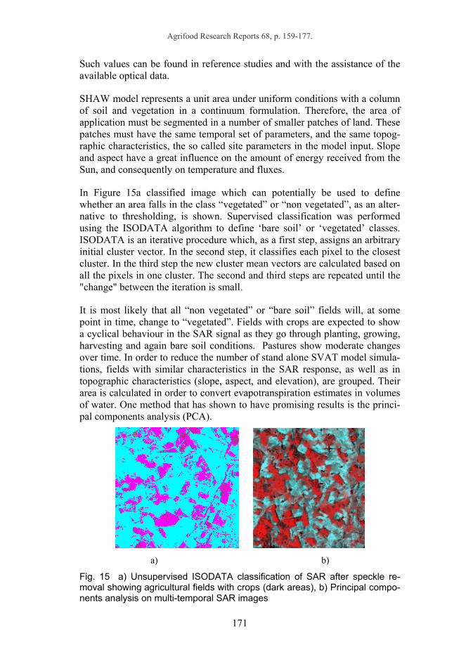
In Figure 15a classified image which can potentially be used to define whether an area falls in the class “vegetated” or “non vegetated”, as an alter-native to thresholding, is shown. Supervised classification was performed using the ISODATA algorithm to define ‘bare soil’ or ‘vegetated’ classes. ISODATA is an iterative procedure which, as a first step, assigns an arbitrary initial cluster vector. In the second step, it classifies each pixel to the closest cluster. In the third step the new cluster mean vectors are calculated based on all the pixels in one cluster. The second and third steps are repeated until the "change" between the iteration is small.

It is most likely that all “non vegetated” or “bare soil” fields will, at some point in time, change to “vegetated”. Fields with crops are expected to show a cyclical behaviour in the SAR signal as they go through planting, growing, harvesting and again bare soil conditions. Pastures show moderate changes over time. In order to reduce the number of stand alone SVAT model simula-tions, fields with similar characteristics in the SAR response, as well as in topographic characteristics (slope, aspect, and elevation), are grouped. Their area is calculated in order to convert evapotranspiration estimates in volumes of water. One method that has shown to have promising results is the princi-pal components analysis (PCA).

a) b)

Fig. 15 a) Unsupervised ISODATA classification of SAR after speckle re-moval showing agricultural fields with crops (dark areas), b) Principal compo-nents analysis on multi-temporal SAR images


172

Principal component analysis is a transformation through rewriting the data with properties the original set did not have. The data may be sufficiently simplified prior to a classification while also removing artefacts such as multi-collinearity. Two interrelated difficulties could hinder the widespread use of SAR imagery in land cover mapping and monitoring: speckle and geo-referencing. Speckle poses problems for both scene segmentation and geo-referencing: high-frequency, spatially random multiplicative noise hinders clustering algorithms. Most de-speckling techniques trade spatial information for noise reduction. Using multiple image dates, noise can be reduced with little loss of spatial resolution. Furthermore, image time series enable assess-ment of land cover variation, whether due to seasonality or disturbance. Prin-cipal component analysis on SAR image series can identify a landscape's dominant spatial-temporal modes of backscattering. The first principal com-ponent yields a very low noise image that contains information about tempo-rally invariant terrain features such as slope and aspect, whereas the second or third can reveal the targeted features of agricultural fields (Figure 15b).

00.050.1

0.150.2

0.250.3

0.350.4

0.450.5

1 2 3 4 5 6 7 8 9

Image acquisition dates

Back

scat

ter v

alue

[lin

ear]

Fig. 16 SAR backscatter mean value change on successive acquisition dates for three different agricultural fields. With a segmentation process, the agricultural fields can easily be delineated. Performing statistical analysis on each of the fields in the area, which exhibit temporal variations due to disturbances (crop growth and harvesting), tempo-ral changes of the mean radar backscatter coefficient can be calculated (Fig-ure 16). The target is the agricultural fields that show strong time dependent response in the signal inferring changes from “crops” to “bare soil” condi-tions. Three images at one time were considered in the analysis, and targeted fields were assigned with a SVAT column at a later stage.

The next step was to determine the minimum and maximum values for plant growth function parameters. Optical images alone, if the required number of images is available (at least once in the growing season of each crop type), or generalisation based on knowledge of land use and agricultural practices in the area can provide reasonable estimates. There are numerous studies pub-


173

lished that relate vegetation indices with plant parameters. One example is the University of Montana database which relates the normalised vegetation index with the leaf area index with thousands of field measurements. LAI is defined as the total one-sided (or one half of the total all-sided) green leaf area per unit ground surface area. It is an important biological parameter be-cause it defines the area that interacts with solar radiation and provides the remote sensing signal. VI’s, on the other hand, have the ability to closely

track the duration and intensity of the canopy photosynthetic capacity, and therefore can be linked with very well established relationships.

4.4.2 Parameter relationships and growth function

The range 200-500 in the SAR intensity images is linear to the vegetation indices with a good accuracy. The value of 500 in SAR image intensity was proposed as a good threshold for the differentiation of land as vegetated or bare soil. Vegetation in the area can be classified as either crops or pastures depending on the temporal change in SAR backscatter. This means that an area which exhibits low mean intensity and low variation is very likely to be covered by permanent pasture. Of particular importance among the plant parameters are the parameters which describe plant structure and growth such as leaf area index, plant height and root depth and above ground biomass.

Published records in Ireland show that land use is 50.2% pastures, 8.1 % rough grazing, 6.8% cereals, 8.5% hay, and 0.2 fruit and horticulture. This can be used as a general guide. More specific information on agricultural production (Table 1) was obtained from the Irish Department of Food and Agriculture (2003).

Table 1. Maximum values of plant root depth and leaf area index

Crop Max. root depth

(m)

Max. LAI

(m²/m²) Barley (Spring) 1.2-1.6 4 - 6 Beans (Dry) 0.9-1.3 3 - 4 Lentils 0.9-1.3 3 - 4 Maize 1.5-2.0 4 - 7 Oats 1.2-1.6 4 - 6 Peas (Dry) 0.9-1.3 3 - 4 Sorghum 1.4-1.8 6 – 10 Soybean 1.4-1.8 4 - 7 Sunflower 1.7-2.2 4 - 5 Wheat (spring) 1.2-1.6 4 - 6 Wheat (winter) 1.5-2.0 5 - 8 Grass (cropped) 0.8 4.0


174

MaizeSoybean

Wheat (winter)

Grass (cropped)

Barley (Spring)

Beans (Dry)

Wheat (spring)

3

4

5

6

7

0.7 0.8 0.9 1 1.1 1.2 1.3 1.4 1.5 1.6 1.7 1.8 1.9 2

Maximum Root Depth [m]

Max

imum

Lea

f Are

a In

dex

Fig. 17. Graphical representation of maximum LAI versus maximum root depth for various crop types.

In the idealised situation that the model simulates, plants may be assumed to vary in leaf area index, plant height, rooting depth, and biomass between a minimum and a maximum value as in Table 1. The minimum can generally be set to zero, and an emphasis is put to the maximum value which can be given to the model with a very good accuracy if some knowledge of the spe-cies exists. Figure 17 is a graphical representation of the relationship between the maximum LAI and maximum rooting depth for the various crop types encountered in the area.

Figure 18 shows a generalised plant growth function of a logarithmic form proposed. One or more model parameters can be multiplied by a factor which is based upon the selection of an appropriate function and a suitable vegeta-tion index derived from satellite data. Different functions can be used based on experimental results obtained by various plant types. The vegetation index can be one of the many developed and used for plant identification and status characterisations.

f(x) = a Ln(x) +b

00.10.20.30.40.50.60.70.80.9

1

0 10 20 30 40 50 60 70 80 90 100

parameter scale factor [% max value](plant height, LAI, root depth, biomass)

Nor

mal

ized

veg

etat

ion

inde

x(N

DV

I,SA

VI,S

AR

inde

x)

Fig. 18. The proposed typical plant growth function based on indices


175

4.4.3 Model calibration for surface temperature

Calibration of vegetation parameters can be based on short period simulations starting under convenient initial conditions with the objective to reproduce land surface temperature estimations obtained from the remotely sensed im-ages. Spatial variation of vegetation properties are defined according to changes in vegetation indices obtained from the visible and near infrared channels. The proportion of the contribution of soil and plants will also be accomplished, based on the principle of the soil adjusted index (SAVI) and the fractional vegetation cover.

Effective full cover for many crops occurs at the initiation of flowering. For row crops where rows commonly interlock leaves such as beans, sugar beets, potatoes and corn, effective cover can be defined as the time when the leaves of plants in adjacent rows begin to intermingle so that soil shading becomes nearly complete, or when plants reach nearly full size if no intermingling occurs. For some crops, especially those taller than 0.5 m, the average frac-tion of the ground surface covered by vegetation (fc) at the start of effective full cover is about 0.7-0.8. Fractions of sunlit and shaded soil and leaves do not change significantly with further growth of the crop beyond fc greater than 0.7 to 0.8. The crop or plant can continue to grow in both height and leaf area after the time of effective full cover. However, it is difficult to determine when densely sown vegetation such as winter and spring cereals and some grasses reach effective full cover. For dense grasses, effective full cover may occur at about 0.10-0.15 m height. For thin strands of grass (rangeland), grass height may approach 0.3-0.5 m before effective full cover is reached. Densely planted forages such as alfalfa and clover reach effective full cover at about 0.3-0.4 m. Another way to estimate the occurrence of effective full cover as a rule of thumb is when the leaf area index (LAI) reaches three.

A plant's temperature usually runs just above air temperature. Plants dissipate heat by long-wave radiation, convection of heat into the air, and transpiration (water loss from leaves). Transpiration is a major mechanism of plant cooling and a means of keeping plant temperatures near air temperatures. Sometimes radiated heat and hot breezes prevent heat dissipation and add to the plant's heat load. Another reason that may add heat is the cooling mechanism through plant transpiration. If parameters are not properly assigned, it is ex-pected that this may lead to lower transpiration. Thus, heat load may in-crease, and a discrepancy from the satellite thermal observations may occur. Through the calibration process, there will be an effort to investigate the parameterisation scheme with comparisons of simulated and observed plant temperatures.

The percentage of vegetation cover, which changes with the leaf area index, can determine the contribution of soil and vegetation to the thermal energy recorded by the satellite. It is important that this distinction is made prior to


176

comparison of simulated and observed temperature values. Areas with vege-tation between ‘bare soil’ conditions and full vegetative cover are expected to lie in between the maximum and minimum temperature values in proportion to these two contributions.

In order to investigate the sensitivity of ET estimation using the SHAW model, as a result of the selection of the parameters that describe the vegeta-tion conditions, some preliminary simulations were carried out and the result-ing ET as a percentage of rainfall for the same period was calculated. The first column in Figure 19 shows the ET from bare soil. The second column was calculated after assigning vegetation with an initial set of parameters. Subsequent columns are produced by changing one or more parameters at a time.

The ability of remotely sensed data to distinguish between “bare soil” areas and “vegetated” areas can have a very positive result in estimating fluxes over space. These ‘bare soil’ areas can have as little as half the ET of devel-oped crop fields. A second important observation is the impact of root depth, as the available water that plants with longer and deeper roots can potentially extract increases significantly with depth.

( )

36.148.6 53.2

71.5 68.257.4 56.8

66.7 59.8

020406080

100

plant albedo 0.1 0.1 0.1 0.1 0.1 0.1 0.1 0.5

leaf w ater -5.0 -5.0 -5.0 -5.0 -5.0 -5 -60 -5

Stom res exp 5.0 5.0 5.0 5.0 5 10 10 10

Min Stomatal 10.0 10.0 10.0 10 100 100 100 100

resist 70000.0 70000.0 70000 120000 120000 120000 120000 120000

root depth 0.1 0.1 0.35 0.35 0.35 0.35 0.35 0.35

Dry Plant Bio 0.5 5 5 5 5 5 5 5

LAI 1.0 4 4 4 4 4 4 4

Fig. 19. Sensitivity of parameter selection on cumulative ET expressed as a percentage of rainfall.

5. Conclusions

The optical images provide a clear delineation of the shapes of the agricul-tural fields, and therefore spatial segmentation is a quite straightforward task. For the SVAT model, the time varying properties of the vegetation cover can be determined from the properties of the radar backscatter values for every field or area in the watershed. Plant growth parameters can be adjusted be-tween minimum and maximum values with a function based on the backscat-ter distribution. The optimum function can be decided upon the agreement of surface temperature with the satellite estimates.


177

With SAR signal and vegetation links established through the processing of satellite data, the medium resolution multi-temporal and multi-spectral SAR and ASTER data provides the basis of model parameterisation. It provides the identification of areas where vegetation indices change over time and their topographic characteristics, which are needed by the SVAT model in order to estimate fluxes. Published plant physiological studies of various species can be used to determine the maximum values of each model parame-ter.

Acknowledgement

This research was carried out within the framework of the European Space Agency Earth Observation Project ‘Land surface moisture distribution and rainfall-runoff processes using remotely sensed data and implications in hy-drologic modelling’, ID number 1226. The authors wish to thank the ESA for making the SAR data used in this project available.

References

Bennett, T.H. 1998. ‘Development and application of a continuous soil mois-ture accounting algorithm for the Hydrologic Engineering Centre Hydro-logic Modelling system (HEC-HMS)’, MSc thesis, Dept. of Civil and Envi-ronmental Engineering, University of California, Davis.

Flerchinger, G. N., W.P. Kustas, & M.A. Weltz. 1998. ‘Simulating surface energy fluxes and radiometric surface temperatures for two arid vegeta-tion communities using the SHAW model’, Journal of Applied Meteorol-ogy. 37:449-460

Irish Department of Food and Agriculture, 2003. http://www.bsyse.wsu.edu/ cropsyst/manual /parameters/crop/morphology.htm#cropmorphtab.

Laur H., Bally P., Meadows P., Sanchez J., Schaettler B. & Lopinto E., 1996. ‘ERS SAR Calibration - Derivation of Backscattering coefficient in ESA ERS SAR PRI Products’, Technical report n ES-TN-RS-PM-HL09, ESA-ESRIN, June 1996.

Mangolini M. & Arino, O. 1996. ‘ERS-SAR and Landsat-TM multitemporal fusion for crop

US Army Corps of Engineers, 2003. ‘HEC Hydrological modeling System’, version 2.1.3.

US Department of Agriculture, 2000. ‘The Simultaneous Heat and Water model’.

hydrological and agro-ecological data acquisition using remotely...

Documents