hydrogen sulfide monitoring near oil and … hydrogen sulfide monitoring near oil and gas production...
TRANSCRIPT
U.S. Department of the Interior Fish & Wildlife Service
Environmental Contaminants Program
by
Joel D. Lusk and Erik A. Kraft U.S. Fish and Wildlife Service
New Mexico Ecological Services Field Office 2105 Osuna Road NE
Albuquerque, New Mexico, USA 87113 Project Identification Number: FFS 2F41- 200220006.1
December 2010
HYDROGEN SULFIDE MONITORING NEAR OIL AND GAS PRODUCTION FACILITIES IN SOUTHEASTERN NEW MEXICO
AND POTENTIAL EFFECTS OF HYDROGEN SULFIDE TO MIGRATORY BIRDS AND OTHER WILDLIFE
ii
Hydrogen Sulfide Monitoring near Oil and Gas Production Facilities in Southeastern New Mexico and Potential Effects of Hydrogen Sulfide to
Migratory Birds and Other Wildlife
by
Joel D. Lusk
and
Erik Kraft
U.S. Fish and Wildlife Service
New Mexico Ecological Services Field Office
2105 Osuna Road NE
Albuquerque, New Mexico
__________________
U.S. Fish and Wildlife Service Region 2 Environmental Contaminants Program
Project Identifier 200220006.1 Federal Financial System #2F41
DISCLAIMER The findings, opinions, conclusions, and recommendations expressed in this report are
those of the authors and have not been formally disseminated by the U.S. Department of the Interior, the Fish and Wildlife Service, or the Bureau of Land Management, and should
not be construed to represent any agency determination or policy. Reference to any specific commercial product, process, or Service by trade name, manufacturer, or
otherwise, does not constitute endorsement or recommendation by the United States
iii
ABSTRACT Hydrogen sulfide (H2S) is a colorless, flammable and highly toxic gas with a characteristic odor of rotten eggs. It is produced naturally and as a result of human activity. Nationally, the largest source of hydrogen sulfide is from petroleum production. We monitored hydrogen sulfide near oil and gas production facilities near the cities of Roswell, Artesia, Hobbs, and Carlsbad in southeastern New Mexico and evaluated its potential effects on migratory birds and other species of wildlife. We deployed hydrogen sulfide monitors in different wildlife habitats near oil and gas production facilities starting November 6, 2002 and concluding August 6, 2003. Concentrations of hydrogen sulfide as high as 33 parts per million (ppm) were measured near the town of Loco Hills, New Mexico, approximately 25 miles (mi) (40 kilometers [km]) east of Artesia, New Mexico. Point count surveys of migratory birds were also conducted to determine differences in habitat use of areas impacted by oil and gas production activities. Point count survey results of migratory birds from undisturbed sites (areas without oil and gas activities within 250 meters) were compared with disturbed sites (areas affected by oil and gas activities). Point count surveys began on November 21, 2002 and concluded on August 6, 2003. We found statistically significant differences in the average number of avian individuals per point count, the average number of avian species per point count, the species diversity, and the average concentration of hydrogen sulfide per point count at disturbed and undisturbed sites. Avian diversity and number of species as determined by point count surveys were significantly lower at disturbed sites than at undisturbed sites. There is little information on the effect of hydrogen sulfide on migratory birds or other wildlife species even though they often occupy habitats that contain elevated hydrogen sulfide in the ambient air. In order to evaluate the toxicity of hydrogen sulfide to a variety of species, we modeled the dose and potential response of the sand dune lizard, as well as several migratory birds and mammal species to hydrogen sulfide. We determined that concentrations as low as 1 ppm may affect highly active migratory birds and mammals. Adoption of ambient hydrogen sulfide air quality standards as low as 1 ppm may be appropriate to protect wildlife.
iv
TABLE OF CONTENTS
List of Figures ............................................................................................................................v List of Tables ........................................................................................................................... vi Introduction ................................................................................................................................1
Hydrogen Sulfide Characteristics ........................................................................................1 Rules and Regulations Governing Hydrogen Sulfide Emissions in New Mexico...............2 Toxicity of Hydrogen Sulfide to Wildlife ............................................................................4
Study Area .................................................................................................................................7 Methods......................................................................................................................................8
Monitoring Site Selection and Characterization ..................................................................8 Avian Survey Methods ........................................................................................................8 Long-term Hydrogen Sulfide Monitoring Methods ............................................................9 Derivation of Wildlife Toxicity Benchmarks ....................................................................10 Determination of Potential Sources of Monitored Hydrogen Sulfide Concentrations ......11
Results ......................................................................................................................................12 Discussion ................................................................................................................................14 Recommendations ....................................................................................................................16 Literature Cited ........................................................................................................................17 Appendices ...................................................................................................................................
Appendix A: Data Set for Undisturbed and Disturbed Sites Including Survey Number, Date, Latitude, Longitude, Total Number of Birds, Number of Species, and Hydrogen Sulfide Concentration for Each Survey ...............55 Appendix B: Data for Undisturbed Sites Including Survey Number and Species Composition for Each Survey .........................................................................63 Appendix C: Data for Disturbed Sites Including Survey Number and Species Composition for Each Survey .........................................................................78
v
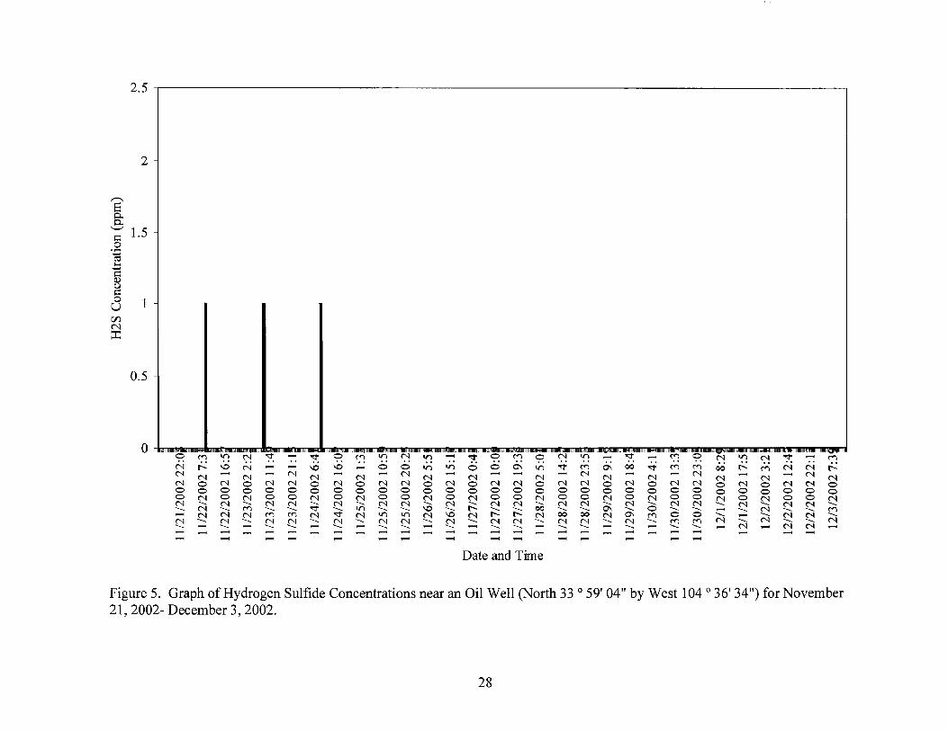
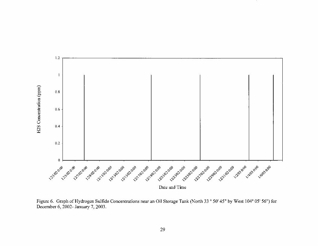
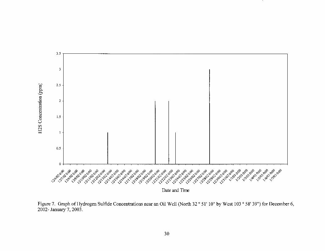
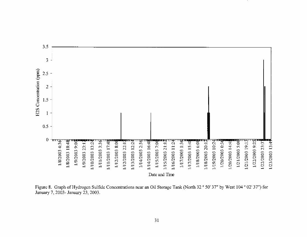
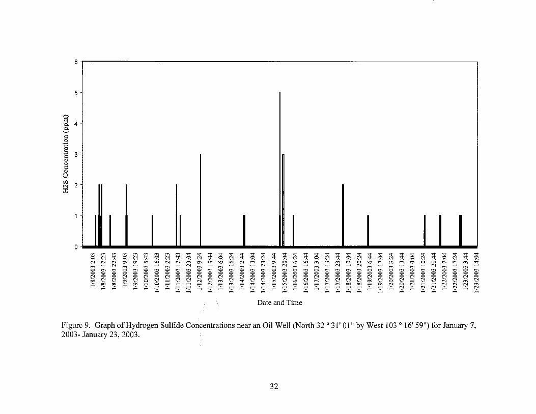
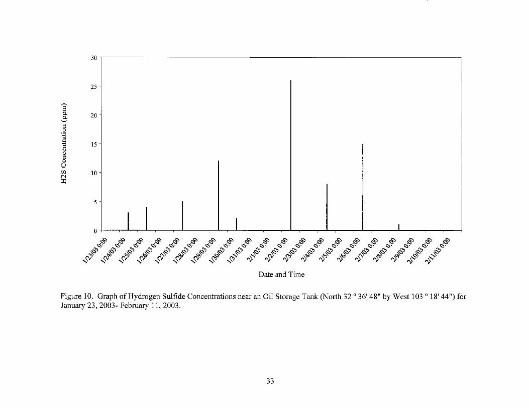
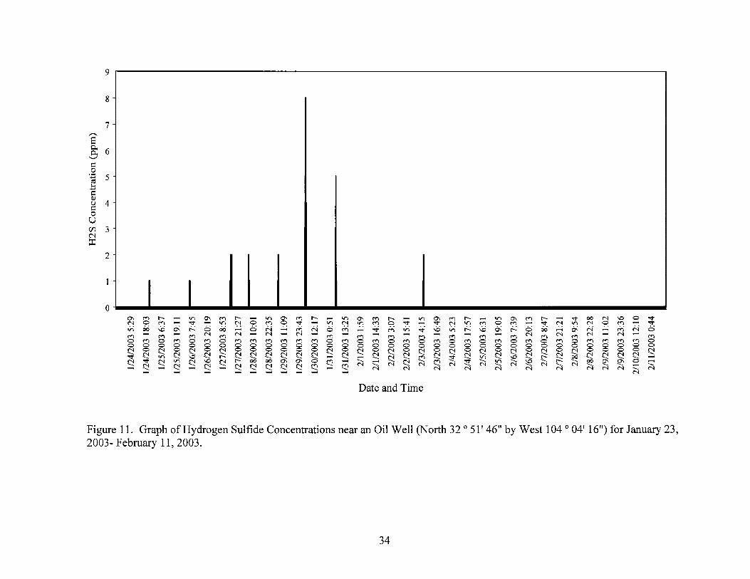
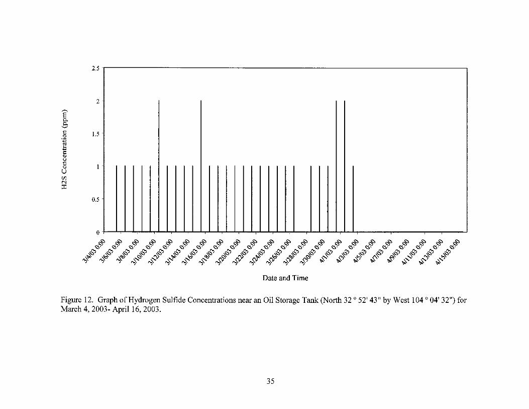
LIST OF FIGURES Figure 1. Map of the Study Area and Hydrogen Sulfide Monitoring Results ...........................24 Figure 2. Graph of Hydrogen Sulfide Concentrations near an Oil Storage Tank (North 32º 50' 10" by West 103 º 58' 39") for November 6, 2002- November 19, 2002. .........25 Figure 3. Graph of Hydrogen Sulfide Concentrations near an Oil Well (North 32 º 27' 05" by West 104 º 31' 29") for November 6, 2002- November 19, 2002. .......26 Figure 4. Graph of Hydrogen Sulfide Concentrations near an Oil Storage Tank (North 32 º 60' 17" by West 104 º 36' 34") for November 21, 2002- December 3, 2002. ........27 Figure 5. Graph of Hydrogen Sulfide Concentrations near an Oil Well (North 33 º 59' 04" by West 104 º 36' 34") for November 21, 2002- December 3, 2002. .........28 Figure 6. Graph of Hydrogen Sulfide Concentrations near an Oil Storage Tank (North 33 º 50' 45" by West 104 º 05' 56") for December 6, 2002- January 7, 2003. ..............29 Figure 7. Graph of Hydrogen Sulfide Concentrations near an Oil Well (North 32 º 51' 10" by West 103 º 58' 39") for December 6, 2002- January 7, 2003. ..............30 Figure 8. Graph of Hydrogen Sulfide Concentrations near an Oil Storage Tank (North 32 º 50' 37" by West 104 º 02' 37") for January 7, 2003- January 23, 2003. ................31 Figure 9. Graph of Hydrogen Sulfide Concentrations near an Oil Well (North 32 º 31' 01" by West 103 º 16' 59") for January 7, 2003- January 23, 2003. ................32 Figure 10. Graph of Hydrogen Sulfide Concentrations near an Oil Storage Tank (North 32 º 36' 48" by West 103 º 18' 44") for January 23, 2003- February 11, 2003. ............33 Figure 11. Graph of Hydrogen Sulfide Concentrations near an Oil Well (North 32 º 51' 46" by West 104 º 04' 16") for January 23, 2003- February 11, 2003. ............34 Figure 12. Graph of Hydrogen Sulfide Concentrations near an Oil Storage Tank (North 32 º 52' 43" by West 104 º 04' 32") for March 4, 2003- April 16, 2003. ......................35 Figure 13. Graph of Hydrogen Sulfide Concentrations near an Oil Well (North 32 º 49' 54" by West 104 º 02' 41") for March 4, 2003- April 16, 2003. ......................36 Figure 14. Graph of Hydrogen Sulfide Concentrations near Mathers Natural Area (North 32 º 48' 14" by West 103 º 56' 27") for April 23, 2003- June 28, 2003. .......................37 Figure 15. Graph of Hydrogen Sulfide Concentrations near an Oil Well (North 32 º 42' 21" by West 103 º 46' 12") for April 23, 2003- June 28, 2003. .......................38
vi
LIST OF FIGURES Continued Figure 16. Graph of Hydrogen Sulfide Concentrations near an Oil Storage Tank (North 32 º 48' 10" by West 103 º 45' 31") for June 28, 2003- August 6, 2003. ......................39 Figure 17. Graph of Hydrogen Sulfide Concentrations near an Oil Well (North 32 º 45' 16" by West 103 º 36' 39") for June 28, 2003- August 6, 2003. ......................40 Figure 18. Graph of Species Composition Present at Undisturbed and Disturbed Sites for the Winter Survey Season. ...........................................................................................41 Figure 19. Graph of Species Composition Present at Undisturbed and Disturbed Sites for the Spring Survey Season .............................................................................................42 Figure 20. Graph of Species Composition Present at Undisturbed and Disturbed Sites for the Summer Survey Season ..........................................................................................43 Figure 21. Graph of Species Composition Present at Undisturbed and Disturbed Sites for the Entire Survey Season ..............................................................................................44 Figure 22. Potential Sources of Hydrogen Sulfide in a “Wind Cone” based on nearby Wind Speed and Direction Towards the Measured Hydrogen Sulfide Concentration .........................45
LIST OF TABLES Table 1. Common and Scientific Names of Selected Wildlife Species found in Sand Shinnery Community of the Mescalero Sands in Southeast New Mexico .................................46 Table 2. Dosimetric Factors for Avian, Mammal and Reptile Species and Calculation of the Hydrogen Sulfide NOAEL, LOAEL and FEL for local Wildlife ....................................49 Table 3. Species Composition of Birds Present at the Disturbed Sites and Undisturbed Sites During the Winter Survey Season from November 21, 20002 to March 21, 2003. ...................51 Table 4. Species Composition of Birds Present at the Disturbed Sites and Undisturbed Sites During the Spring Survey Season from March 21, 2003 to June 21, 2003. ...............................52 Table 5. Species Composition of Birds Present at the Disturbed Sites and Undisturbed Sites During the Summer Survey Season from to June 21, 2003to August 6, 2003. ..........................53 Table 6. Species Composition of Birds Present at the Disturbed Sites and Undisturbed Sites from November 21, 20002 to August 6, 2003. ...........................................................................54
1
INTRODUCTION
Petroleum is a thick, flammable mixture of gaseous, liquid, and solid hydrocarbons that occurs naturally beneath the earth's surface. During extraction, petroleum is brought to the surface and transported to refineries where it is separated into liquid and gas fractions including natural gas, gasoline, kerosene, lubricating oils, paraffin wax, and asphalt (U.S. Environmental Protection Agency [USEPA] 1999). Hydrogen sulfide is found naturally in underground petroleum reserves. Hydrogen sulfide may be emitted or released during exploration, development, extraction, treatment and storage, transportation and refining of petroleum products (USEPA 1993).
In New Mexico, Dubyk et al. (2002), monitored ambient hydrogen sulfide levels and reported the highest concentrations (0 to 15 ppm) around oil and gas facilities near the Black River northeast of Whites City, New Mexico. In this region, Sias and Snell (1998) also had reported moribund wildlife species (e.g., owls and other raptors) as well as carapace remains of turtles near oil and gas wells that were known to emit hydrogen sulfide and other gases. Sias and Snell (1998) suggested that since some reptiles were strongly associated with the bottoms of dune valleys in the area, then these reptiles may be more susceptible to gas poisoning since hydrogen sulfide is heavier than air. The U.S. Fish and Wildlife Service (Service) was requested to review the available information to determine the risks posed to wildlife from local hydrogen sulfide emissions.
There are no Federal or State rules that identify protective air quality standards specifically to protect wildlife. There is little information on the effect of hydrogen sulfide on migratory birds or other wildlife species even though they often occupy habitats that contain elevated hydrogen sulfide in the ambient air. The Service therefore initiated this investigation (in conjunction with the New Mexico Department of Game and Fish and the U.S. Bureau of Land Management [BLM]) in order to determine: 1) the ambient concentrations in areas associated with oil and gas activities as well as in areas without that activity; 2) determine and associate the density, diversity or composition of the avian community in these two types of areas; 3) empirically test hydrogen sulfide toxicity to animals in a laboratory setting; and 4) identify whether measured hydrogen sulfide concentrations pose a risk to wildlife and which guilds of animals may be sensitive to hydrogen sulfide exposures in southeastern New Mexico. Note that Objective 3; the laboratory toxicity testing was not conducted due to lack of funding.
Hydrogen Sulfide Characteristics
Hydrogen sulfide (Chemical Abstract Service Registration Number 7783-06-4) is a colorless, flammable and highly toxic gas with a characteristic odor of rotten eggs. It is produced naturally and as a result of human activity (USEPA 1993). Natural sources include anaerobic bacterial reduction of sulfates and sulfur-containing organic compounds. Organic matter almost always contains sulfur and wherever it undergoes putrefaction (such as at the bottom of a lake, deep underground, in piles of manure, during decomposition, etc.), some of that sulfur is converted to hydrogen sulfide. Hydrogen sulfide is also found in crude petroleum,
2
natural gas, volcanic gases, stagnant, thermal or polluted waters, livestock manure, coal pits and in springs (USEPA 1993).
Hydrogen sulfide is soluble in both water and oil and as a result can move great distances before conditions favor its emergence as a vapor. Hydrogen sulfide may evaporate from surface water, depending on temperature and pH. Because hydrogen sulfide vapor is heavier than air, it may also creep along the ground for a distance before being neutralized by chemical reactions, ignited, and it may pool in low-lying areas in the environment (USEPA 1993).
During petroleum extraction activities, impurities like hydrogen sulfide, water, sand, silt, or additives used to enhance extraction, are removed or allowed to volatilize into the air. In addition to hydrogen sulfide emission during petroleum production and refining, accidental air releases of hydrogen sulfide can occur through leaking tubing, valves, tanks, pipeline ruptures or open pits (USEPA 1993). During spills or leaks, hydrogen sulfide gas can volatilize to the atmosphere before clean up. Releases to the environment are primarily by emissions into ambient air, where the hydrogen sulfide is likely to remain for less than 1 day, but may persist for as long as 42 days in cold climates (Agency for Toxic Substances and Disease Registry [ATSDR] 2004). The concentrations of hydrogen sulfide in air in unpolluted areas are low (ATSDR 2004), with areas that have natural sources ranging between 0.1 and 0.3 parts per billion (ppb). Hydrogen sulfide is unlikely to bioconcentrate or biomagnify in the food chain, and has not been found to cause cancer (ATSDR 2004).
Hydrogen sulfide is corrosive; therefore, it is desirable to remove hydrogen sulfide during the petroleum conditioning process and during wastewater treatment (USEPA 1991). Hydrogen sulfide emission can occur during petroleum production and refining, through pipeline ruptures or leaking tubing, valves, flanges, tanks, and open pits (USEPA 1993). When natural gas is produced from the well that is not sold or used on-site, it can be flared or vented, thereby releasing carbon monoxide, nitrogen oxides, hydrogen sulfide, or sulfur dioxide to the atmosphere.
Rules and Regulations Governing Hydrogen Sulfide Emissions in New Mexico
The Clean Air Act requires the USEPA to set National Ambient Air Quality Standards for pollutants considered harmful to public health and the environment. Toxic air pollutants are known or suspected to cause cancer or other serious health effects, such as reproductive effects or birth defects, or adverse environmental effects. The USEPA regulates emissions of toxic air pollutants from industrial sources referred to as “source categories." Hydrogen sulfide was originally listed as a toxic air pollutant for which the USEPA was to assess the hazards to public health and the environment resulting from the emission of hydrogen sulfide associated with the extraction of oil and natural gas (USEPA 1993). However, it was later noted that a clerical error led to the inadvertent inclusion of hydrogen sulfide on the list of toxic air pollutants and it was removed (USEPA 1993). There are no national standards regulating hydrogen sulfide.

3
The New Mexico Environment Department (NMED) Air Quality Bureau has adopted 0.010 ppm as the ambient air quality standard for hydrogen sulfide (NMED 2002). However, Part 20.2.3.110.B(2) of the New Mexico Annotated Code (NMAC) identifies a regional air quality standard for hydrogen sulfide in the Pecos-Permian Basin (30-minute [min] average) as 0.100 ppm. The Pecos-Permian Basin Intrastate Air Quality Control Region is composed of Quay, Curry, De Baca, Roosevelt, Chaves, Lea, and Eddy Counties in New Mexico. Also, the ambient air quality standard for hydrogen sulfide is 0.03 ppm (30-min average) within corporate limits of municipalities in the Pecos-Permian Basin Intrastate Air Quality Control Region or within 5 mi (8 km) of the corporate limits of municipalities having a population of greater than twenty thousand. However, there are no requirements for monitoring hydrogen sulfide emissions from any new source or from the net increase of hydrogen sulfide emissions where these emissions could cause ambient concentrations to exceed the air quality standards in New Mexico unless those emissions exceed 10 tons of sulfur per year from a stationary source (20.2.74.502 NMAC). The New Mexico Oil Conservation Division of the Energy, Minerals, and Natural Resources Department (EMNRD) has promulgated rules regarding the emission of hydrogen sulfide from any well or gas-producing facility in New Mexico (EMNRD 2001). These rules provide for the protection of the public’s safety in areas where hydrogen sulfide concentrations are greater than 100 ppm. Generally, any gas-processing facility where hydrogen sulfide is present at concentrations of 100 ppm or more must take reasonable measures to forewarn and safeguard people that have occasion to be on or near the area. Wells drilled where there is substantial probability of people encountering hydrogen sulfide gas in concentrations of 500 ppm or more must have warning “poison gas” signs. Facilities (except gas-processing plants) having storage tanks with hydrogen sulfide gas in concentrations of 1,000 ppm or more must have identifying signs indicating the specific protective measures that may be necessary to protect public safety. Any well, lease, or processing plant handling gas with a hydrogen sulfide concentration and volume that equates to 10,000 cubic feet (ft3) (283 cubic meters [m3]) per day or more, which is located within 0.25 mi (0.4 km) of a dwelling, public place, or highway, must install safety devices and maintain them in operable conditions or establish safety procedures designed to prevent the undetected escape of hydrogen sulfide as well as prepare a contingency plan for people’s safe evacuation. The BLM has applied rules and regulations for well leases and facilities on all BLM lands in New Mexico (43 Code of Federal Regulations [CFR] 3160; see BLM 1991). The BLM has identified areas or zones they manage for oil and gas production (along with other resource uses and goals), where postings must occur and human entry must be accompanied by monitoring devices to reduce the risk of hydrogen sulfide exposure (BLM 1997). The BLM has also identified, mapped, and posted signs in areas where elevated hydrogen sulfide releases from oil and gas wells are known to occur that may pose risks to human health and safety in New Mexico (BLM 1997). Most gas emissions are minimized through prevention (i.e., preventive maintenance and occasional monitoring, inspections, leak detection and notification systems, installation of catalytic converters, filters, sponges, routine replacement of gaskets, seals, valves, tightening
4
connections, and welding, as well as educating and informing the workforce)(USEPA 1993). Flaring or burning off gases may sometimes be used to reduce air emissions that are unavoidable. Nearly all oil and gas production wells are equipped with a vent or flare to release unusual pressure, and some wells that produce only a small amount of natural gas will vent or flare it when there is no on-site use for the gas (e.g., to power engines), no pipeline nearby to transport the gas to market, and no regulations regarding its disposal (USEPA 1993). Since natural gas has economic value, flaring is usually considered a last resort. When a gas is flared, it passes through the vent away from the well, and is burned in the presence of a pilot light. Although it is preferable to prevent the emission in the first place, flaring has benefits over simple venting of unburned material. However, the practice of flaring also produces sulfur dioxide, which is a regulated air pollutant (USEPA 1993). Toxicity of Hydrogen Sulfide to Wildlife There are no Federal or State rules that identify protective air quality standards for wildlife. Few studies address the risks posed to wildlife from hydrogen sulfide emissions. One investigation by Siegel et al. (1986) examined the ambient levels of hydrogen sulfide at Sulphur Bay Wildlife Area in New Zealand where shorebirds were exposed to hydrogen sulfide of geothermal origin at concentrations of 0.13 to 3.9 ppm. They found fewer species of birds used this habitat compared to similar wetlands without detectable levels of hydrogen sulfide. However, no parameters of exposure were measured at either the population level or the individual level. The Canadian Wildlife Service also conducted a study of the effects of a gas well blowout in Alberta, Canada on wildlife (New Norway Scientific Committee 1974). Concentrations between 5 and 10 ppm were documented and birds and small animals were absent from the study area after the blowout. The New Norway Scientific Committee (1974) suggested that low concentrations of hydrogen sulfide, as low as 5 to 10 ppm, negatively affect habitat usage by avian species. Data on the effects of hydrogen sulfide are only well documented for common test animals and humans (ATDSR 2004). The following information on human toxicity was included because the mechanism of hydrogen sulfide toxicity is considered to be common among all vertebrates that utilize aerobic pathways of metabolism (USEPA 2003; U.S. National Library of Medicine [USNLM] 2003). The characteristics of acute hydrogen sulfide toxicity are dependent on the concentration and duration of exposure. Exposure is usually by inhalation. At high concentrations (250-500 ppm), hydrogen sulfide acts as a respiratory irritant, which can lead to a pulmonary edema (USEPA 2003; USNLM 2003). At higher concentrations (500-1,000 ppm), hydrogen sulfide acts as a systemic poison, causing unconsciousness and death by respiratory paralysis in minutes (USNLM 2003). Long-term damage and death in small mammals occurs when hydrogen sulfide gas levels exceed 50-100 parts per million (ppm) (Dahme et al. 1983). A single 4-hour exposure to hydrogen sulfide concentrations of 15-100 ppm may cause eye irritation and conjunctivitis (“gas eye”), convulsions and pulmonary edema in rodents (Lopez et al. 1989). At concentrations ranging from 10 to 25 ppm people report flu-like symptoms including headaches, dizziness, nausea, vomiting, irritation of the eyes, nose and throat, fatigue, insomnia, and digestive disturbances (National Institute for Occupational Safety and Health [NIOSH] 1977). The health effects of chronic,
5
low-level exposure to hydrogen sulfide to wildlife or humans, however, are not well defined (USEPA 2003; ATSDR 2004). After inhalation, hydrogen sulfide enters the circulation directly across the alveolar-capillary membrane where it dissociates into a sulfide ion (USNLM 2003). The sulfide ion is then selectively taken up by the brainstem where it interferes with neurotransmitter levels and also reversibly interacts with a number of enzymes, proteins, including hemoglobin and myoglobin. Sulfide ions will bind to cytochrome-oxidase within mitochondria, thereby blocking electron transport leading to metabolic acidosis to cytotoxic anoxia, and finally, cell death (Smith 1991). As a cellular poison, the effects of hydrogen sulfide are seen across all organ systems and would be expected to behave similarly in all vertebrate species that utilize aerobic metabolism such as in migratory birds, mammals, certain reptiles and amphibians (Dombkowski et al. 2005).
Hydrogen sulfide has been recently identified as vasoactive (i.e., affecting the blood vessels) in all vertebrate classes of mammals, birds, reptiles and fish (Dombkowski et al. 2005). When isolated blood vessels were exposed to hydrogen sulfide vasoactivity was observed including constriction, dilation, and multiphasic responses that were both species- and vessel-specific (Dombkowski et al. 2005). The ability of hydrogen sulfide to serve as either (or both) a vasoconstrictor or vasodilator is an evolutionary feature for regulation of vasoactivity that seems to have been exploited by nearly all vertebrates (Dombkowski et al. 2005). As a result, hydrogen sulfide may trigger a “startle” response in exposed wildlife by constricting blood vessels, increasing heart rate and blood pressure with a consequent increase in respiration and glucocorticoid release (Gabrielsen and Smith 1995, Maren 1999).
Olfactory Toxicity
The olfactory toxicity of hydrogen sulfide exposure deserves special emphasis for wildlife because their chemical senses such as odor detection are well-developed to detect food, danger, or potential mates (Geist 2000; Rehorek et al. 2000; Getchell and Getchell 2005; Lledo et al. 2005). In most terrestrial vertebrates, the vomeronasal organ is a dome-shaped, cartilage-encased nasal chemosensory structure found on the rostral floor in the nasal cavity (Rehorek et al. 2000). The vomeronasal organ is an important interface between the environment and the central nervous system (Rehorek et al. 2000). Sensory perception is a process by which information from the external world is subsequently reformatted into an internal state, so this organ is responsible for correctly coding sensory information from thousands of odorous chemicals and other stimuli to the brain (Lledo et al. 2005). Snakes are thought to possess the most complex vomeronasal organs. Odorous compounds, even when present at concentrations that cannot be consciously detected by people, often produce a distinct response in a variety of animals (Roth and Goodwin 2002).
For land animals, the initial step in olfactory response involves the interaction of an odor, usually a volatile organic molecule, with specific receptors located on the surface of the olfactory sensory neurons that penetrate the skull and terminate in the olfactory bulb at the base of the brain (Roth and Goodwin 2002). After entering, odorants dissolve in the mucous lining, bind to specific receptors on the neuron’s cilia, which opens various ion channels and
6
depolarizing the membranes of sensory neurons sending various signals throughout the brain (Mombaerts 1999). There are substantial animal toxicology data demonstrating damage to the olfactory senses by airborne chemicals (Cowart et al. 1997), and particularly due to hydrogen sulfide exposure (USEPA 2003; ATSDR 2004).
In the derivation of the reference concentration (RfC) used for the Integrated Risk Information System, the USEPA (2003) used the results of a study by Brenneman et al. (2000) that exposed 10-week old male rats to 0, 10, 30, or 80 ppm hydrogen sulfide for 6 hours per day for 10 weeks. At the end of the exposure period, the noses of the animals were dissected, sectioned and histological evaluations were made of the respiratory and olfactory epithelium. Lesions were observed in the olfactory mucosa in the animals exposed to 30 or 80 ppm hydrogen sulfide (Brenneman et al. 2000). The critical effects in the Brenneman et al. (2000) study were nasal lesions of the olfactory mucosa; with 30 ppm identified as the Lowest-Observable-Adverse-Effect Level (LOAEL), 10 ppm identified as the No-Observable-Adverse-Effects-Level (NOAEL), 100 ppm identified as the Frank-Effects Level (FEL) by the USEPA (2003) in their derivation of the RfC. Lopez et al. (1987) and Moulin et al. (2002) identified that the olfactory epithelium was more sensitive to the toxic effects of hydrogen sulfide than the respiratory epithelium. Credence for the hypothesis that hydrogen sulfide specifically impacts the olfactory senses is supported by the correlation between hydrogen sulfide flux and the human nasal response to hydrogen sulfide odor (USEPA 2003).
In humans, the odor threshold begins at 0.003-0.3 ppm, is easily perceptible at 1 ppm, and is reminiscent of rotten eggs at 3-30 ppm (ATSDR 2004). A sickeningly sweet odor is described from 30-100 ppm above which rapid olfactory fatigue and paralysis ends perception (ATSDR 2004). Prolonged exposure to low concentrations may also result in olfactory paralysis or nasal membrane necrosis (USNLM 2003). Compared with animals, humans have a relatively small area of olfactory epithelium (USEPA 2003).
Reptiles, birds and mammals posses one or more pairs of cartilaginous, epithelially covered projections within the nasal cavity know as turbinates (Geist 2000). In reptiles, these turbinates are relatively simple structures associated with olfaction, however, with birds and mammals, these turbinates are relatively elaborate convoluted structures lined with moist mucociliated epithelium (Geist 2000). Respiratory turbinates are situated directly in the path of respiratory airflow. As inspired air passes through the nasal cavities and over the moist surfaces of the respiratory turbinates, heat and water are exchanged – as is hydrogen sulfide (Geist 2000).
After passing through the nasal passages, inspired air passes down the trachea and through to the main respiratory organ of mammals, birds and reptiles. The trachea consists of repeatedly branching longitudinal and transverse tubes and ducts that terminate in numerous blind-ending sacs or alveoli in the lungs of terrestrial animals. The respiratory organs of mammals, birds, and reptiles are very different from each other (Bennett 1973; Brown et al. 1997). However, these structural differences and the differences in ventilation rates for these different classes of animals (mammals, birds and reptiles) can be used to account for the relative inhalation dose of hydrogen sulfide and therefore, the derivation of an inhalation reference concentration for animals (USEPA 1994).
7
STUDY AREA
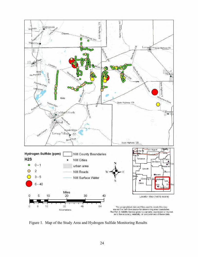
The study area includes portions of Chaves, Eddy, and Lea Counties in southeastern New Mexico (Figure 1). Generally, the study area includes the areas known as the Southern High Plains, the lower Pecos River drainage basin, the Caprock, and the Mescalero Sands (also known as the Shinnery Sands Ecoregion). The Mescalero Sands are an extensive deep-sand dune area west of the Caprock, south of State Highway 70, north of State Highway 31, and east of the Pecos River (Griffith et al. 2006). Portions of the Mescalero Sands have been designated as a National Natural Landmark, an Outstanding Natural Area, and a Research Natural Area (BLM 1997). Hawley (1986) identified this area as part of the Great Plains Province, while Dick-Peddie (1993) further identified this area as Plains-Mesa Sand Scrub due to the presence of shin oak (Quercus havardii). This region also contains extensive petroleum resources of the Permian Basin that annually produce over 65 million barrels (7.5 million m3) of crude oil and over 550 trillion ft3 (15.6 trillion m3) of natural gas (EMNRD 2000). Irrigated farming occurs along the Pecos River in lower Chaves and Eddy Counties.
Associated with the Mescalero Sands is a community of plants and animals called a “sand shinnery” (Peterson and Boyd 1998). Shin oaks co-dominate the sand shinnery vegetative community along with sand sagebrush (Artemisia filifolia), tall grasses and forbs. These shin oaks comprise the largest stand of oaks in the United States and occupy nearly six million acres in northern Texas, western Oklahoma, and southeast New Mexico. This shin oak forest is only 1 to 4 ft (0.3 to 1.2 m) tall and is composed of ancient plants, most of them hundreds to thousands of years old (Peterson and Boyd 1998). Two wildlife species characteristic of the sand shinnery include the lesser prairie-chicken (Tympanuchus pallidicinctus), known for its courtship rituals, and the sand dune lizard (Sceloporus arenicolus). Both of these species are candidates for listing under the Endangered Species Act as their population declines have been attributed to habitat loss and degradation (Taylor 1980; Service 1998; Painter et al. 1999). Common avian species in the study area such as mourning dove, scaled quail, red-tailed hawk, and common roadrunner were described by Peterson and Boyd (1998). Table 1 lists these wildlife species and others found in the area along with their scientific names.
8
METHODS
Monitoring Site Selection and Characterization
Areas that were selected for monitoring or for bird surveys were characterized as “disturbed” if they were within ~80 to 100 ft (25 to 30 meters [m]) of any visible well pads, drilling rigs, oil storage tanks, pipelines or oil pumps. Often there was a distinct change in the vegetative community near the well pads, tanks, pipelines or pumps as the vegetation was cleared, or was distinctly different from the surrounding area. Areas were characterized as “undisturbed” if they were at least 800 to 1000 ft (~250 to 300 m) from any visible well pads, storage tanks, pipelines or processing facilities and the vegetation community appeared homogenous in all directions (except for roads – see below). We employed a survey technique recommended by Ralph (1993) that included the systematic placement bird survey point counts at designated distances along roads or trails rather than random sampling design. Site selection for surveys and handheld hydrogen sulfide monitoring was conducted by access along tertiary roads (i.e., often unpaved County roads). A systematic grid of points along tertiary roads was implemented. A randomization program was used to choose those tertiary roads among those available. Thereafter the distance between survey locations was set at approximately every 0.6 mi (~1,000 m) as gauged by an odometer or as measured using a global positioning system (GPS; Garmin, Model GPS V, Olathe, Kansas. The GPS was Wide Area Augmentation System-enabled, set to degrees, minutes and seconds using the 1983 North American Datum). This GPS was also used to mark the location of all observations. The process of driving along roads and stopping approximately every 0.6 mi (1,000 m) was repeated until at least eight bird surveys with eight hydrogen sulfide measurements with a handheld hydrogen sulfide gas detector were conducted each from disturbed and undisturbed sites.
Avian Survey Methods
Few studies have measured natural or accidental exposure of wildlife to hydrogen sulfide. Additionally, few studies have been conducted on bird communities in areas associated with the extensive oil and gas activities in southeast New Mexico. In this study, we quantified the concentrations of hydrogen sulfide in the environment using long-term stationary and hand-held monitors in conjunction with point count surveys of the avian community. A point count is a total of all the birds detected visually and aurally by an observer from a fixed station during a fixed period of time (Ralph et al. 1993, 1995; Hamel et al. 1996; Huff et al. 2000). We used point counts to determine the presence or absence of bird species and their number along with our characterization of the landscape as either “disturbed” or “undisturbed” by oil and gas activities. Note that we did not quantify the area’s vegetation within the observational point count area (i.e., vegetation species, number, or spatial extent).
Point count bird surveys were conducted along tertiary roads as described above. Point count surveys began on November 21, 2002 and concluded on August 6, 2003. Counts lasted 3 to 5 min and survey sites consisted of a circle with a radius of approximately 164 ft (50 m). Initial tests of the statistical differences in the point count results from either 3- or 5-min
9
point count surveys of similar habitats showed no detectable difference (t-test, P = 0.69). Once the survey started, all birds that were seen or heard by a trained observer within the point count circle were recorded. The total number of birds, number of species, and number of individuals of each species were recorded. Using a handheld hydrogen sulfide monitor (Industrial Scientific, Model HS560, Oakdale, Pennsylvania), the average concentration of hydrogen sulfide was also recorded from measurements before, during and after the bird survey. Bird surveys were conducted during winter, spring and summer (but not in autumn), as migratory bird community composition changes with season, however, surveys were not repeated in the same areas during each season (winter, spring and summer).
To test for differences between hydrogen sulfide data and bird habitat use we conducted point count surveys of birds in areas that we classified as disturbed or undisturbed by oil and gas activities and season. For each season and for each habitat classification, the number of birds, the number of species, and the number of individuals of each species were summed. Then the average number of birds per point count, the average number of species per point count, the average number of individuals of each species per point count, and the average concentration of hydrogen sulfide gas per point count location were calculated. For each season, the differences in the average number of birds per point count, the average number of species per point count, and the average concentration of hydrogen sulfide gas at the disturbed sites and the undisturbed sites were determined with the use of t-tests (Schefler 1969). For each season and the study overall, differences between the average numbers of individuals of each species per point count for each habitat type were determined with the use of an rXc contingency table (Schefler 1969). The statistical threshold of acceptability that was used was P ≤ 0.05 (Schefler 1969).
Long-term Hydrogen Sulfide Monitoring Methods Site selection for hand-held hydrogen sulfide monitoring was as described above. However, three sites were preselected for long-term monitoring based on site characteristics. Long-term monitoring occurred northwest of Carlsbad, New Mexico, due to concerns reported by the community for hydrogen sulfide odors; west of Tatum, New Mexico, as the reference condition; and near Maljamar, New Mexico. For the long-term monitoring of hydrogen sulfide, an Odalog H2S Gas Logger (App-Tek International Proprietary Limited, Munich, Germany) was attached to a nearby shrub at approximately 3 ft (~1 m) in height using a chain and lock. The monitors were placed as close as possible (less than 50 ft [15 m]) to oil and gas equipment within disturbed sites and over 1,000 ft (300 m) away from any such equipment at the undisturbed site. The hydrogen sulfide monitors contained a data logger that recorded the hydrogen sulfide concentration to within 1 ppm once every minute. The monitors were cleaned and inspected every 2 to 4 weeks, data were downloaded onto a laptop computer and batteries changed prior to placement at a new site. Monitors were calibrated according to manufacturer’s specifications and data were later downloaded and then imported into a spreadsheet for graphic representation. Data collection of long-term hydrogen sulfide monitoring began on November 6, 2002 and concluded on August 6, 2003.
10
Derivation of Wildlife Toxicity Benchmarks
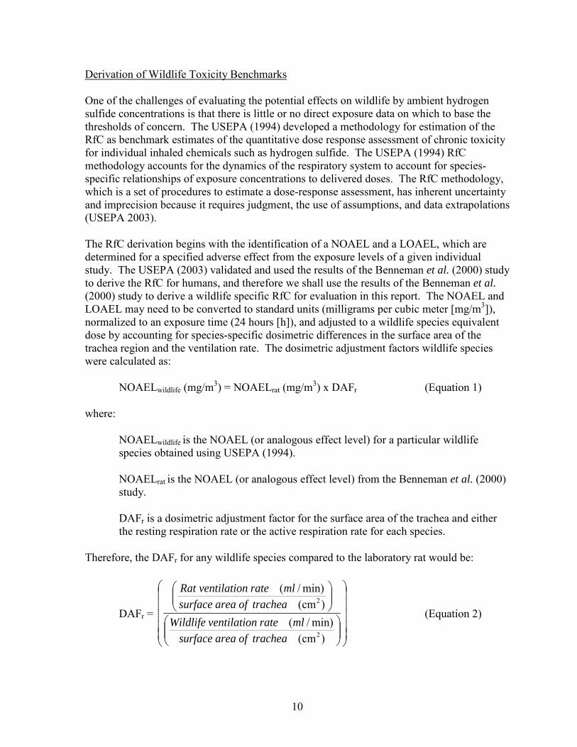
One of the challenges of evaluating the potential effects on wildlife by ambient hydrogen sulfide concentrations is that there is little or no direct exposure data on which to base the thresholds of concern. The USEPA (1994) developed a methodology for estimation of the RfC as benchmark estimates of the quantitative dose response assessment of chronic toxicity for individual inhaled chemicals such as hydrogen sulfide. The USEPA (1994) RfC methodology accounts for the dynamics of the respiratory system to account for species-specific relationships of exposure concentrations to delivered doses. The RfC methodology, which is a set of procedures to estimate a dose-response assessment, has inherent uncertainty and imprecision because it requires judgment, the use of assumptions, and data extrapolations (USEPA 2003).
The RfC derivation begins with the identification of a NOAEL and a LOAEL, which are determined for a specified adverse effect from the exposure levels of a given individual study. The USEPA (2003) validated and used the results of the Benneman et al. (2000) study to derive the RfC for humans, and therefore we shall use the results of the Benneman et al. (2000) study to derive a wildlife specific RfC for evaluation in this report. The NOAEL and LOAEL may need to be converted to standard units (milligrams per cubic meter [mg/m3]), normalized to an exposure time (24 hours [h]), and adjusted to a wildlife species equivalent dose by accounting for species-specific dosimetric differences in the surface area of the trachea region and the ventilation rate. The dosimetric adjustment factors wildlife species were calculated as:
NOAELwildlife (mg/m3) = NOAELrat (mg/m3) x DAFr (Equation 1)
where:
NOAELwildlife is the NOAEL (or analogous effect level) for a particular wildlife species obtained using USEPA (1994).
NOAELrat is the NOAEL (or analogous effect level) from the Benneman et al. (2000) study.
DAFr is a dosimetric adjustment factor for the surface area of the trachea and either the resting respiration rate or the active respiration rate for each species.
Therefore, the DAFr for any wildlife species compared to the laboratory rat would be:
DAFr =
)cm(min)/(
)cm(min)/(
2
2
tracheaofareasurfacemlratenventilatioWildlife
tracheaofareasurfacemlratenventilatioRat
(Equation 2)
11
The ventilation rates and surface area of the laboratory rat were reported by the USEPA (1994). However, ventilation rates and trachea dimensions area in wildlife species are a function of body mass (Calder 1968; Hinds and Calder 1971; Bennett 1973; Brown et al. 1997; Frappell et al. 2001). We used the avian body masses reported by Dunning (1993) and Sell (1977) as well as the mammalian body masses reported and Silva and Downing (1995) to calculate the ventilation rates and trachea surface area while active or at rest (Table 2). However, while respiration rates for various reptile species was reported by Bennett (1973), and body mass was reported by Degenhardt et al. (1996), information on trachea surface area was not available. Therefore, we made an assumption that sand dune lizard trachea dimensions were equivalent to that of a bird of equal mass (0.005 kilograms [kg]). Then we used geometry to determine the surface area of the trachea. We assumed the trachea radius was one half the trachea width and the surface area was equal to that of a cylinder with a circumference of 2 times the trachea radius times pi (2πr) times the height that is equal to that of the trachea length (Table 2). Note that if hydrogen sulfide toxicity is not related to exposure by ventilation, but rather by species-specific differences in gas exchange surfaces, then this dose scaling may not be appropriate. Calculation of a protective air quality standard for wildlife would require the development of an RfC using uncertainty factors to account for species differences, laboratory-to-field study modifiers, and duration of exposure. We compared the ambient concentrations of hydrogen sulfide to the NOAEL to indicate potential risks to wildlife. The lowest NOAEL concentration was rounded to an integer and that value was recommended as an interim ambient air quality recommendation to protect wildlife until an RfC could be further developed. These interim ambient air quality recommendations are therefore “action levels” as they do not consider a number of uncertainty factors normally used to derive ambient air quality criteria (USEPA 1994, 2003) Determination of Potential Sources of Monitored Hydrogen Sulfide Concentrations For those two events when hydrogen sulfide concentrations exceeded 5 ppm during our long-term monitoring, we evaluated the nearby wind speed and direction for the hour at which the elevated hydrogen sulfide concentration was measured to determine potential source(s). Wind data at the monitoring device was unavailable; therefore we obtained hourly wind speed and direction from a nearby weather station in Roswell, New Mexico (NOAA 2003) and assumed they were representative. For example, when wind speeds and direction were reported at 17 mi/h (~27 km/h) from the north, we assumed that the measured hydrogen sulfide concentrations came from sources in an upwind cone up to 17 mi (24 km) in length were the most likely sources of the hydrogen sulfide concentrations measured.
12
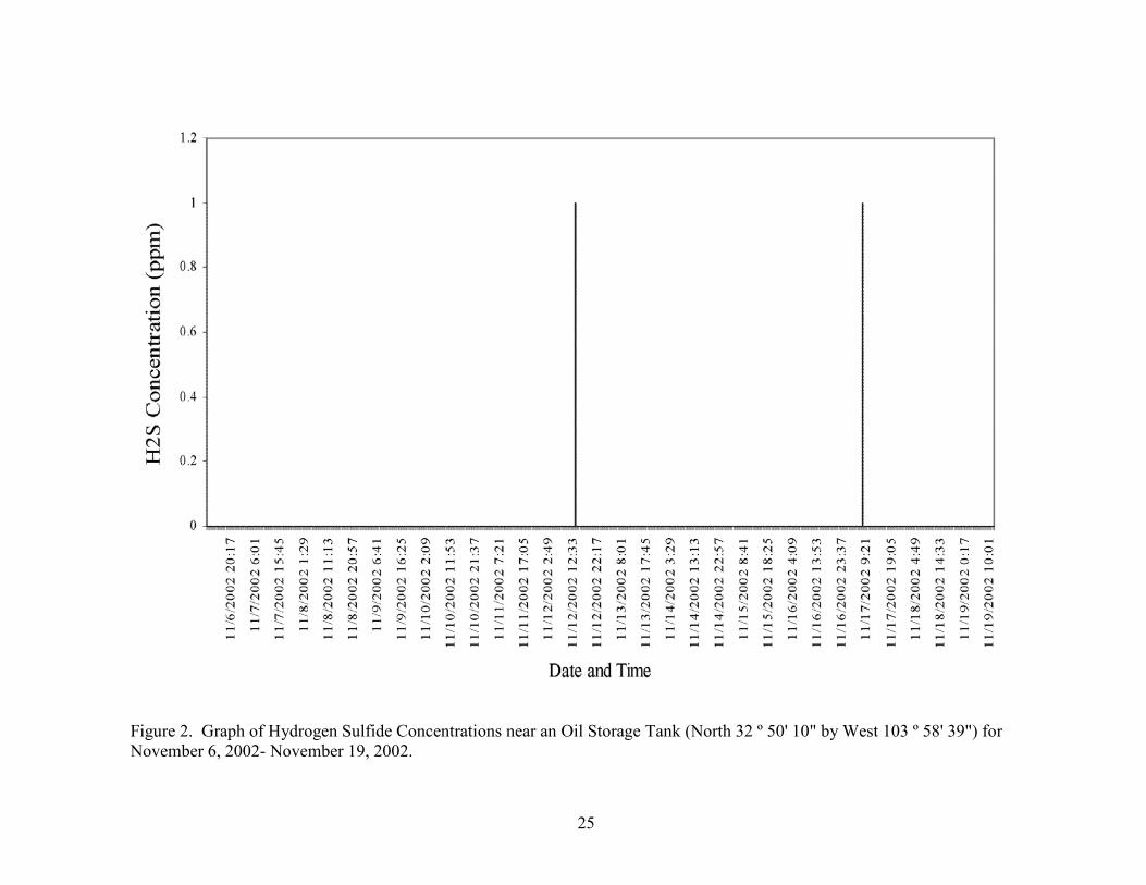
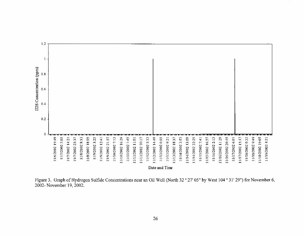
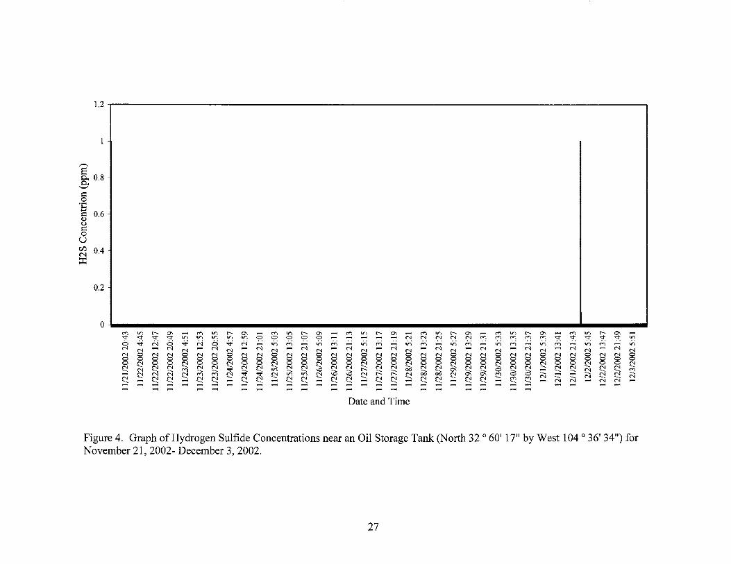
RESULTS
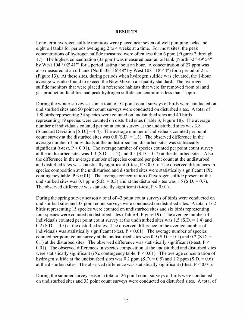
Long term hydrogen sulfide monitors were placed near seven oil well pumping jacks and eight oil tanks for periods averaging 2 to 4 weeks at a time. For most sites, the peak concentrations of hydrogen sulfide measured were often less than 6 ppm (Figures 2 through 17). The highest concentration (33 ppm) was measured near an oil tank (North 32 º 49' 54" by West 104 º 02' 41") for a period lasting about an hour. A concentration of 27 ppm was also measured at an oil tank (North 32º 36' 48" by West 103 º 18' 44") for a period of 2 h. (Figure 13). At these sites, during periods when hydrogen sulfide was elevated, the 1-hour average was also found to exceed the New Mexico air quality standard. The hydrogen sulfide monitors that were placed in reference habitats that were far removed from oil and gas production facilities had peak hydrogen sulfide concentrations less than 1 ppm. During the winter survey season, a total of 52 point count surveys of birds were conducted on undisturbed sites and 50 point count surveys were conducted on disturbed sites. A total of 198 birds representing 34 species were counted on undisturbed sites and 40 birds representing 19 species were counted on disturbed sites (Table 3, Figure 18). The average number of individuals counted per point count survey at the undisturbed sites was 3.8 (Standard Deviation [S.D.] = 4.4). The average number of individuals counted per point count survey at the disturbed sites was 0.8 (S.D. = 1.3). The observed difference in the average number of individuals at the undisturbed and disturbed sites was statistically significant (t-test, P < 0.01). The average number of species counted per point count survey at the undisturbed sites was 1.3 (S.D. = 1.2) and 0.5 (S.D. = 0.7) at the disturbed sites. Also the difference in the average number of species counted per point count at the undisturbed and disturbed sites was statistically significant (t-test, P < 0.01). The observed differences in species composition at the undisturbed and disturbed sites were statistically significant (rXc contingency table, P < 0.01). The average concentration of hydrogen sulfide present at the undisturbed sites was 0.1 ppm (S.D. = 0.3) and at the disturbed sites was 1.5 (S.D. = 0.7). The observed difference was statistically significant (t-test, P < 0.01). During the spring survey season a total of 42 point count surveys of birds were conducted on undisturbed sites and 33 point count surveys were conducted on disturbed sites. A total of 62 birds representing 15 species were counted on undisturbed sites and six birds representing four species were counted on disturbed sites (Table 4, Figure 19). The average number of individuals counted per point count survey at the undisturbed sites was 1.5 (S.D. = 1.4) and 0.2 (S.D. = 0.5) at the disturbed sites. The observed difference in the average number of individuals was statistically significant (t-test, P < 0.01). The average number of species counted per point count survey at the undisturbed sites was 0.9 (S.D. = 0.1) and 0.2 (S.D. = 0.1) at the disturbed sites. The observed difference was statistically significant (t-test, P < 0.01). The observed differences in species composition at the undisturbed and disturbed sites were statistically significant (rXc contingency table, P < 0.01). The average concentration of hydrogen sulfide at the undisturbed sites was 0.2 ppm (S.D. = 0.5) and 1.2 ppm (S.D. = 0.6) at the disturbed sites. The observed difference was statistically significant (t-test, P < 0.01). During the summer survey season a total of 26 point count surveys of birds were conducted on undisturbed sites and 33 point count surveys were conducted on disturbed sites. A total of
13
54 birds representing 15 species were counted on undisturbed sites and 15 birds representing five species were counted on disturbed sites (Table 5, Figure 20). The average number of individuals counted per point count survey at the undisturbed sites was 2.1 (S.D. = 2.3) and 0.5 (S.D. = 0.8) at the disturbed sites. The observed difference in the average number of individuals was statistically significant (t-test, P < 0.01). The average number of species counted per point count survey at the undisturbed sites was 0.9 (S.D. = 0.1) and 0.3 (S.D. = 0.5) at the disturbed sites. The observed difference was statistically significant (t-test, P < 0.01). The observed differences in species composition at the undisturbed and disturbed sites were statistically significant (rXc contingency table, P < 0.01). The average concentration of hydrogen sulfide at the undisturbed sites was 0.3 ppm (S.D. = 0.5) and 2.0 ppm (S.D. = 1.6) at the disturbed sites. The observed difference was statistically significant (t-test, P < 0.01). Overall, a total of 120 point count surveys of birds were conducted on undisturbed sites and 116 point count surveys were conducted on disturbed sites. A total of 314 birds representing 40 species were counted on undisturbed sites and 58 birds representing 25 species were counted on disturbed sites (Table 6, Figure 21). Lesser prairie-chickens were not observed at any of the study sites. The average number of individuals counted per point count survey at the undisturbed sites was 2.6 (S.D. = 3.3) and 0.5 (S.D. = 0.9) at the disturbed sites. The observed difference was statistically significant (t-test, P < 0.01). The average number of species counted per point count survey at the undisturbed sites was 1.1 (S.D. = 0.9) and 0.4 (S.D. = 0.6) at the disturbed sites. The observed difference was statistically significant (t-test, P < 0.01). The observed differences in species composition at the undisturbed and disturbed sites were statistically significant (rXc contingency table, P = 0.04). The average concentration of hydrogen sulfide at the undisturbed sites was 0.2 ppm (S.D. = 0.4) and 1.6 ppm (S.D. = 1.1) at the disturbed sites. The difference was statistically significant (t-test, P < 0.01).
14
DISCUSSION Dubyk et al. (2002), monitored ambient hydrogen sulfide levels in areas of New Mexico near these facilities: 1) a sewage treatment plant; 2) four dairy operations; 3) a poultry operation; 4) a liquid septage disposal facility; 5) a sewage sludge disposal facility; and, 6) nine oil and gas facilities. All of the facilities they inspected indicated a high likelihood that they could exceed the New Mexico air quality standards for hydrogen sulfide. At oil and gas facilities, hydrogen sulfide concentrations ranged from 0 to 15 ppm; the highest concentrations were reported near the Black River northeast of Whites City, New Mexico. Dubyk et al. (2002) reported that all other facilities were measured with ambient concentrations less than 0.11 ppm. Dubyk et al. (2002) also reported that background ambient air concentrations of hydrogen sulfide in New Mexico range from 0 to 0.010 ppm and averaged 0.0057 ppm. We measured concentrations of hydrogen sulfide as high as 33 ppm near an oil tank in the vicinity of Loco Hills, New Mexico, approximately 25 mi (40 km) east of Artesia, New Mexico. Using wind speed and direction, oil production wells and injection wells were identified upwind of the elevated hydrogen sulfide concentrations detected by the long-term monitors (Figure 22). However, it is uncertain if any of these particular production or injection wells were the source of the measured hydrogen sulfide peak concentrations in the ambient air. Based on our dosimetric calculations, mammals appeared to be more sensitive to hydrogen sulfide toxicity than either birds or reptiles. Reptile ventilation rates are slower and therefore reduce the amount of hydrogen sulfide exposure to their tissues. Hydrogen sulfide concentrations less than 2 ppm appear not to pose a risk to mammal species at rest, while concentrations greater than 5 ppm pose a risk to wildlife and are likely to affect their olfactory senses, irritate their eyes and mucus membranes, or dilate their blood vessels and cause a startle or stress reaction (Table 2). Mammals exposed to greater than 11 ppm would be more likely to flee an area or succumb to hydrogen sulfide toxicity (Table 2). Avian species are more at risk when they are active or flying as they inhale deeper. Hydrogen sulfide concentrations less than 1 ppm would appear not to pose a risk to birds when they are active or flying (Table 2). Hydrogen sulfide concentrations less than 8 ppm appear not to pose a risk to avian species at rest, while concentrations greater than 25 ppm pose a risk to avian species and may affect their olfactory senses, irritate their eyes and mucus membranes, or dilate their blood vessels and cause a startle or stress reaction (Table 2). Based on these analyses, ambient air hydrogen sulfide concentrations should be less than 1 ppm to protect flying birds and less than 2 ppm to protect resting mammals from hydrogen sulfide toxicity in their habitat. These recommendations would be considered “action levels” as they do not consider a number of uncertainty factors normally used in the derivation of ambient air quality criteria (USEPA 1994, 2003).
Sias and Snell (1998) hypothesized that since sand dune lizards are strongly associated with the bottoms of dune valleys, these lizards may be more susceptible to gas poisoning (than other lizard species) associated with these wells since hydrogen sulfide is heavier than air. Sias and Snell (1996, 1998) provided data and evidence to conclude that the presence of oil
15
and gas wells is strongly correlated with a reduction in sand dune lizard abundance. Their plots within 263 ft (80 m) of an oil or gas well pad (the area of disturbance around a well) had a 39 percent reduction in the population of sand dune lizards compared with plots more than 623 ft (190 m) from an oil or gas well pad. Sias and Snell (1998) also identified impacts to other wildlife including observations of moribund owls and other raptors as well as they found the carapace remains of turtle carcasses (e.g. turtle shells) in areas around oil and gas wells that were reported to emit hydrogen sulfide and other gases (identified by signage).
We found that sand dune lizards that are active should begin to demonstrate adverse effects at concentrations in their environment greater than 14 ppm. On February 2, 2003, we measured hydrogen sulfide concentrations as high as 26 ppm for 1 h in the early evening (Figure 22) with little or no wind measured nearby. On March 25, 2003, we measured hydrogen sulfide concentrations as high as 33 ppm for 32 min in the early morning with winds measured nearby approaching 17 mi/h (~27 km/h) from the north (Figure 22). These ambient concentrations during these periods were at levels that would be expected to have adverse effects on active sand dune lizards and perhaps other wildlife species as well (Table 2). Sand dune lizards that are resting should be protected from adverse effects of hydrogen sulfide if concentrations in their environment remain below 50 ppm. No ambient hydrogen sulfide concentrations above 50 ppm were measured during this study.
Other studies have found that habitat disrupted by oil and gas activities negatively impacts populations of birds. Migration routes of waterfowl are often changed and the breeding success of waterfowl decreases as a result of oil and gas activities (Monda et al. 1994; Johnson 1998). Populations of birds of prey dramatically decrease when oil wells are placed within habitat they occupy (Squires et al. 1993; Van Horn 1993). Many species of passerines have also been impacted negatively by the building of oil well sites (Baker 1987).
In this study, there was a statistical difference in the average number of individuals counted per point count, the average number of species counted per point count survey, the species composition, and the average concentration of hydrogen sulfide at the undisturbed and the disturbed sites. This suggests that habitat quality may be affected by oil and gas activities and may alter the composition of local avian communities. Habitat disrupted by oil and gas activities favored avian species adapted to feeding in disturbed habitat such as doves, quail, and sparrows. Habitat disturbed by oil and gas activities contained fewer species and reduced usage by species such as wrens, vireos, flycatchers and phoebes. It is possible that oil and gas activities may negatively affect avian diversity and their numbers through changes in vegetation that were not quantified during this study. However, we found that changes in habitat conditions as described as “disturbed” by oil and gas activities, were significantly related to reduced numbers of birds observed during point counts, decreased avian species diversity observed during point counts, and increased hydrogen sulfide concentrations. Nonetheless, the causes of the decline of bird density, diversity and elevated hydrogen sulfide were not determined during this study. Further long-term studies of the effects of oil and gas activities on migratory birds and their habitat are needed. Restoration of habitat affected by activities of oil and gas is needed to preserve migratory bird populations and avian species diversity.
16
RECOMMENDATIONS The authors recommend that Federal, State and Tribal agencies implement the following actions to protect wildlife:
1. Adopt an interim air quality standard of 1 ppm hydrogen sulfide to protect wildlife.
2. Require monitoring of hydrogen sulfide to identify sources in areas where ambient concentrations routinely exceed 1 ppm and find ways to reduce those sources. Routine monitoring should include appropriate meteorological monitoring, particularly local wind conditions and direction, so as to identify any seasonal or geographic trends. Hydrogen sulfide monitoring programs should be adequate to characterize a geographic area and its ambient conditions over time, as well as be able to identify any local sources for management actions.
3. Report incidences of migratory bird deaths to the Service, as may occur when birds
are affected by oil and gas activities, hydrogen sulfide emissions or release of other hazardous fluids. Federal, State and Tribal agencies should identify any means and measures necessary to avoid or minimize the potential for take of migratory birds.
4. Fund studies that confirm the toxicity and mechanisms of action of hydrogen sulfide using mammal, avian and reptile species in order to refine this risk assessment in this study as well as identify any adverse effects to their olfactory tissues and functions.
5. Routinely monitor avian communities in habitats that are affected by oil and gas
activities in order to determine any long-term deleterious trends and develop management strategies to address those trends to conserve migratory bird habitats.
6. Evaluate the changes to the vegetative community by oil and gas activities and any
associated surface waters for effects to migratory birds, and other wildlife.
17
LITERATURE CITED Agency for Toxic Substances and Disease Registry (ATDSR). 2004. Draft toxicological
profile for hydrogen sulfide. United States Department of Health and Human Services, Agency for Toxic Substances and Disease Registry Toxicological Profile for Public Comment, Atlanta, Georgia.
American Ornithologists' Union (AOU). 1998. Check-list of North American Birds. 7th
edition. American Ornithologists' Union, Washington, D.C. http://www.aou.org/checklist/north/index.php. Accessed July 28, 2010.
Baker, W.J. 1987. The effects of oil well sites on forest species of birds. Dissertation,
Western Michigan University, Kalamazoo, Michigan. Bennett, A.F. 1973. Ventilation in two species of lizards during rest and activity.
Comparative Biochemistry and Physiology 46A:653-671. Brenneman, K.A., R.A. James, E.A. Gross, and D.C. Gorman. 2000. Olfactory neuron loss
in adult male CD rats following subchronic inhalation exposure to hydrogen sulfide. Toxicologic Pathology 30:200-208.
Brown, R.E., J.D. Brain, and N. Wang. 1997. The avian respiratory system: A unique
model for studies of respiratory toxicosis and for monitoring air quality. Environmental Health Perspectives 105:188-200.
Bureau of Land Management (BLM). 1991. Code of Federal Regulations at 43 CFR 3160
and 36 CFR 228 Subpart E; Onshore Oil and Gas Order No. 6, Hydrogen Sulfide Operations. Federal Register 55:48958-48988. http://www.blm.gov/pgdata/etc/medialib/blm/co/programs/oil_and_gas.Par.30146.File.dat/ord6.pdf Accessed July 28, 2010.
Bureau of Land Management (BLM). 1997. Roswell resource area proposed resource
management plan/final environmental impact statement. U.S. Department of the Interior, Bureau of Land Management, Roswell District Office, Report BLM-NM-PT-97-003-1610. Roswell, New Mexico. Accessed July 28, 2010. http://www.blm.gov/nm/st/en/fo/Roswell_Field_Office/roswell_rmp_1997.html.
Burrell, G.A., and F.M. Seibert. 1916. Gases found in coal mines. Miner's Circular 14.
Bureau of Mines, U.S. Department of the Interior. Washington, D.C. Calder, W.A. 1968. Respiratory and heart rates of birds at rest. Condor 70:358-365. Collins, J.T. and T.W. Taggart. 2009. Standard common and current scientific names for
North American amphibians, turtles, reptiles, and crocodilians. 6th Edition. Publication of the Center for North American Herpetology, Lawrence, Kansas. www.cnah.org/pdf_files/1246.pdf. Accessed July 28, 2010.
18
Cowart, B.J., I.M. Young, R.S. Feldman, and L.D. Lowry. 1997. Clinical disorders of smell
and taste. Occupational Medicine: State of the Art Reviews 12:465-483. Dahme, E., T. Bilzer, and G. Dirksen. 1983. Zur neuropathologie der jauchegasvergiftung
beim rind (Neuropathology of hydrogen sulfide gas poisioning in cattle). Deutsch Tieraerztle Wochenschribe 90:316-320.
Degenhardt, W.G., C.W. Painter, and A.H. Price. 1996. The amphibians and reptiles of New
Mexico. University of New Mexico Press, Albuquerque, New Mexico. Dick-Peddie, W.A. 1993. New Mexico vegetation, past, present, and future. University of
New Mexico Press, Albuquerque, New Mexico. Dombkowski, R.A., M.J. Russell, A.A. Schulman, M.M. Doellman, and K.R. Olson. 2005.
Vertebrate phylogeny of hydrogen sulfide vasoactivity. American Journal of Physiology: Regulatory, Integrative and Comparative Physiology 288:R243-R252.
Dubyk, S., S. Mustafa, and A. Graham. 2002. Trip Report: H2S Survey, March 18-22,
2002. New Mexico Environment Department, Air Quality Bureau, Santa Fe, New Mexico.
Dunning, J.B. 1993. Handbook of avian body weights. CRC Press, Orlando, Florida. Energy, Minerals, and Natural Resources Department (EMNRD). 2009. New Mexico’s
Energy, Minerals, and Natural Resources Department. Annual Report 2009. Energy, Minerals, and Natural Resources Department, Santa Fe, New Mexico. http://www.emnrd.state.nm.us/MMD/Publications/2009AnlRpt.htm. Accessed July 28, 2010.
Frappell, P.B., D.S. Hinds, and D.F. Boggs. 2001. Scaling of respiratory variables and the
breathing pattern in birds: An allometric and phylogenetic approach. Physiological and Biochemical Zoology 74:75-89.
Frey, J.K., S.O. MacDonald, and J.A. Cook. 2006. Checklist of New Mexico mammals.
Museum of Southwestern Biology, University of New Mexico, Albuquerque, New Mexico. http://web.nmsu.edu/~jfrey/NM%20mammal%20checklist%202006.PDF. Accessed July 28, 2010.
Gabrielsen, G.W., and E.N. Smith. 1995. Physiological responses of wildlife to disturbance.
Pages 95-107 in R.L. Knight and K.J. Gutzwiller, editors. Wildlife and recreationists: Coexistence through management and research. Island Press, Washington, D.C.
Geist, N.R. 2000. Nasal respiratory turbinate function in birds. Physiological and
Biochemical Zoology 73:581-589.
19
Getchell, M.L., and T.V. Getchell. 2005. Fine structural aspects of secretion and extrinsic innervations in the olfactory mucosa. Microscopy Research and Technique 23:111-127.
Griffin, G.E., J.M. Omernik, M.M. McGraw, G.Z. Jacobi, C.M. Canavan, T.S. Schrader, D.
Mercer, R. Hill, and B.C. Moran. 2006. Ecoregions of New Mexico (color poster with map, text, tables and photographs): Reston, Virginia, U.S. Geological Survey (map scale 1:1,400,000. http://www.epa.gov/wed/pages/ecoregions/nm_eco.htm. Accessed July 28, 2010.
Hamel, P.B., W.P. Smith, D.J. Twedt, J.R. Woehr, E. Morris, R.B. Hamilton, and R.J.
Cooper. 1996. A land manager’s guide to point counts of birds in the Southeast. U.S. Department of Agriculture, Forest Service, Southern Forest Experiment Station, Report No. GTR-SO-120, New Orleans, Louisiana. http://ww.treesearch.fs.fed.us/pubs/1594. Accessed July 28, 2010.
Hawley, J.W. 1986. Physiographic provinces I. Pages 23-25 in J.L. Williams, editor. New
Mexico in Maps. University of New Mexico Press, Albuquerque, New Mexico. Hinds, D.S., and W.A. Calder. 1971. Tracheal dead space in the respiration of birds.
Evolution 25:429-440. Huff, M.H., K.A. Bettinger, H.L. Ferguson, M.J. Brown, and B. Altman. 2000. A habitat
based point count protocol for terrestrial birds, emphasizing Washington and Oregon. United States Department of Agriculture, Forest Service, Pacific Northwest Research Station, General Technical Report PNW-GTR-501, Portland, Oregon. http://www.treesearch.fs.fed.us/pubs/2928. Accessed July 28, 2010.
Johnson, S.R. 1998. Distribution and movements of brood-rearing lesser snow geese in
relation to petroleum development in Arctic Alaska. Arctic 51:336-344. Lledo, P.M., G. Gheusi and J.D.Vincent. 2005. Information processing in the mammalian
olfactory system. Physiological Reviews 85:281-317. Lopez, A., M.G. Prior, S. Yong, M. Albassam , and L.E. Lillie. 1987. Biochemical and
cytologic alterations in the respiratory tract of rats exposed for 4 hours to hydrogen sulfide. Fundamentals of Applied Toxicology 9:753-762.
Lopez, A., M.G. Prior, R.J. Reiffenstein, and L.R. Goodwin. 1989. Peracute effects of
inhaled hydrogen sulfide and injected sodium hydrosulfide on the lungs of rats. Fundamentals of Applied Toxicology 12:367-373.
Maren, S. 1999. Long-term potentiation in the amygdala: A mechanism for emotional
learning and memory. Trends in Neurosciences 22:561-567.
20
Mombaerts, P. 1999. Molecular Biology of Odorant Receptors in Vertebrates. Annual Review of Neuroscience 22: 487-509.
Monda, M.J., J.T. Ratti, and T.R. McCabe. 1994. Behavioral responses of nesting tundra
swans to human disturbance and implications for nest predation on the Arctic National Wildlife Refuge. Trumpter Swan Society Newsletter 14:178.
Moulin, F.J., K.A. Brenneman, J.S. Kimbell, and D.C. Dorman. 2002. Predicted regional
flux of hydrogen sulfide correlates with distribution of nasal olfactory lesions in rats. Toxicological Sciences 66:7-15.
New Mexico Annotated Code (NMAC). 2008. Part 19.15.3.118. Natural Resources and
Wildlife. Oil and Gas. Hydrogen Sulfide Gas. http://ww.nmcpr.state.nm.us/NMAC/parts/title19/19.015.0011.htm. Accessed July 28, 2010.
New Mexico Environment Department (NMED). 2002. Part 20.2.3 New Mexico Annotated
Code: Environmental protection. Air Quality (Statewide). Ambient Air Quality Standards. New Mexico Environment Department Air Quality Bureau, Santa Fe, New Mexico. http://www.nmenv.state.nm.us/aqb/regs/20_2_03NMAC_090606.pdf.
New Norway Scientific Committee. 1974. Report of New Norway Scientific Committee
regarding a gas well blowout, October 2, 1973, near Camrose. Alberta Environment Department, Edmonton, Alberta.
National Institute for Occupational Safety and Health (NIOSH). 1977. Criteria for a
recommended standard: occupational exposure to hydrogen sulfide. Publication No. 77-158. U.S. Department of Health, Education, and Welfare. National Institute for Occupational Safety and Health. Washing D.C. http://www.cdc.gov/niosh/77-158.html. Accessed July 28, 2010.
National Oceanic and Atmospheric Administration (NOAA). 2003. Unedited Local
Climatological Data Hourly Observations Table for Roswell Industrial Air Center Airport, Roswell, NM. U.S. Department of Commerce, National Oceanic and Atmospheric Administration. National Climatic Data Center, Ashville, North Carolina. http://cdo.ncdc.noaa.gov/ulcd/ULCD. Accessed July 28, 2010.
Painter, C.W., D.S. Sias, L.E. Fitzgerald, L.L.S. Pierce, and H.L. Snell. 1999. Management
plan for the sand dune lizard, Sceloporus arenicolus, in New Mexico. New Mexico Department of Game and Fish, Santa Fe, New Mexico.
Peterson, R.S., and C.S. Boyd. 1998. Ecology and management of sand shinnery
communities: A literature review. Report RMRS-GTR-16. U.S. Department of Agriculture, Rocky Mountain Research Station, Fort Collins, Colorado. http://www.fs.fed.us/rm/pubs/rmrs_gtr016.html. Accessed July 28, 2010.
21
Ralph, C.J. 1993. Designing and implementing a monitoring program and the standards for
conducting point counts. Pages 204-207 in D.M. Finch and P.W. Stangel, editors. Status and management of neotropical migratory birds: September 21-25, 1992, Estes Park, Colorado. Report GTR-RM-229. U.S. Department. of Agriculture, Forest Service. Rocky Mountain Forest and Range Experiment Station. Fort Collins, Colorado. http://www.treesearch.fs.fed.us/pubs/22900. Accessed July 28, 2010.
Ralph, C.J., G.R. Geupel, P. Pyle, T.E. Martin, and D.F. DeSante. 1993. Handbook of field
methods for monitoring land birds. Report PSW-GTR-144. U.S. Department of Agriculture, Forest Service, Pacific Research Station. Albany, California. http://www.treesearch.fs.fed.us/pubs/3639. Accessed July 28, 2010.
Ralph, C.J., S. Droege, and J.R. Sauer. 1995. Managing and monitoring birds using point
counts: standards and applications. Pages 161-168 in C.J. Ralph, J.R. Sauer, and S Droege, technical editors. Monitoring bird populations by point counts. Report PSW-GTR-149. U.S. Department of Agriculture, Forest Service, Pacific Southwest Research Station Albany, California. http://www.treesearch.fs.fed.us/pubs/31755. Accessed July 28, 2010.
Rehorek, S.J., B.T. Firth, and M.N. Hutchinson. 2000. The structure of the nasal
chemosensory system in squamate reptiles. Lubricatory capacity of the vomeronasal organ. Journal of Biosciences 25:181-190.
Roth, S., and V. Goodwin. 2002. Health effects of hydrogen sulphide: knowledge gaps.
Alberta Environment Publication No. T/696, Edmonton, Alberta. http://environment.gov.ab.ca/info/library/6708.pdf. Accessed July 28, 2010.
Schefler, W.C. 1969. Statistics for the biological sciences. Addison-Wesley Press,
Madison, Wisconsin. Sell, D. 1977. Use of heavily grazed range by breeding lesser prairie chicken females.
Proceedings of the 12th Conference of the Prairie Grouse Technical Council, Pierre, South Dakota.
Sias, D. L., and H. L. Snell. 1996. The dunes sagebrush lizard Sceloporus arenicolus and
sympatric reptile species in the vicinity of oil and gas wells in southeastern New Mexico. Report Final Contract No. 80-516.6-01. University of New Mexico, Albuquerque, New Mexico.
Sias, D. L., and H. L. Snell. 1998. The sand dune lizard Sceloporus arenicolus and oil and
gas development in southeastern New Mexico: Final report of field studies 1995-1997. Final Report Contract No. 80-516.6-01. University of New Mexico, Albuquerque, New Mexcio.
22
Siegel, S.M., P. Penny, B.Z. Siegel, and D. Penny. 1986. Atmospheric hydrogen sulfide levels at the Sulphur Bay Wildlife Area, Lake Rotorua, New Zealand. Water, Air, and Soil Pollution 28: 385-391.
Silva, M.B., and J.A. Downing. 1995. CRC handbook of mammalian body masses. CRC
Press, Boca Raton, Florida. Smith, R.P. 1991. Toxic response of the blood. Pages 257-281 in M.O. Ambur, J. Doull,
and C.D. Klassen, editors. Cassarett and Doull’s Toxicology, The basic science of poisons, 4th edition. Pergamon Press, New York, New York.
Squires, J.R., S.H. Anderson, and R. Oakeleaf. 1993. Home range size and habitat-use
patterns of nesting prairie falcons near oil developments in north eastern Wyoming. Journal of Field Ornithology 64:1-10.
Taylor, M.A. 1980. Status, ecology, and management of the lesser prairie chicken. General
Technical Bulletin RM-77. U.S. Department of Agriculture. Forest Service, Fort Collins, Colorado.
U.S. National Library of Medicine (USNLM). 2010. Hydrogen Sulfide. Hazardous
Substances Database (HSDB) database search using 7783-06-4 on TOXNET. U.S. Department of Health & Human Services, National Library of Medicine, Bethesda, Maryland. http://toxnet.nlm.nih.gov/cgi-bin/sis/search/f?./temp/~37kOAW:1. Accessed August 30, 2010.
U.S. Environmental Protection Agency (USEPA). 1991. Hydrogen sulfide corrosion in
wastewater collection and treatment systems: U.S. Environmental Protection Agency, Office of Water Technical Report 430/09-91-010, Washington, D.C. http://nepis.epa.gov/Exe/ZyPURL.cgi?Dockey=20011KMS.txt. Accessed July 28, 2010.
U.S. Environmental Protection Agency (USEPA). 1993. Report to Congress on hydrogen
sulfide air emissions associated with the extraction of oil and natural gas. Report EPA-453-R-93-045. U.S. Environmental Protection Agency, Washington, D.C. http://nepis.epa.gov/Exe/ZyPURL.cgi?Dockey=00002WG3.txt. Accessed July 28, 2010.
U.S. Environmental Protection Agency (USEPA). 1994. Methods for derivation of
inhalation reference concentrations (RfCs) and application of inhalation dosimetry. Report EPA/600/8-90/066F. U.S. Environmental Protection Agency, Office of Research and Development, Office of Health and Environmental Assessment, Washington, D.C. http://cfpub.epa.gov/ncea/cfm/recordisplay.cfm?deid=71993. Accessed July 28, 2010.
23
U.S. Environmental Protection Agency (USEPA). 1999. EPA Office of Compliance Sector Notebook Project. Profile of the oil and gas extraction industry. Report EPA/310-R-99-006. U.S. Environmental Protection Agency, Washington, D.C. http://www.epa.gov/compliance/resources/publications/assistance/sectors/notebooks/oil.html. Accessed July 28, 2010.
U.S. Environmental Protection Agency (USEPA). 2003. Toxicological review of hydrogen
sulfide (CAS No. 7783-06-4) in support of summary information on the Integrated Risk Information System (IRIS). Report EPA/635/R-03/005. U.S. Environmental Protection Agency, Washington, D.C. http://www.epa.gov/IRIS/toxreviews/0061tr.pdf. Accessed July 28, 2010.
U.S. Fish and Wildlife Service (Service). 1998. Endangered and threatened wildlife and
plants; 12-month finding for a petition to list the Lesser Prairie-Chicken as threatened and designate critical habitat. Federal Register 63:31400-31406.
Van Horn, R. C. 1993. A summary of reproductive success and mortality in a disturbed
ferruginous hawk (Buteo regalis) population in north central Montana, 1990-92 (Abstract). Journal of Raptor Research 27:94.
24
Figure 1. Map of the Study Area and Hydrogen Sulfide Monitoring Results
25
Figure 2. Graph of Hydrogen Sulfide Concentrations near an Oil Storage Tank (North 32 º 50' 10" by West 103 º 58' 39") for November 6, 2002- November 19, 2002.
1
0.9
0.8
--;::;· 0""' .. :::::: 0... 5 0.6
:::::: 0 ..... ....... ~ ;...; ~
0.5
v 0 ,..... 8 0.-t u VJ. ('1 :::r:: 0.3
0.1
0.1
0
Date and Time
Figure 14. Graph of Hydrogen Sulfide Concentrations near Mathers Natural Area (North 32° 48' 14" by West 103° 56' 27") for April23, 2003- June 28, 2003. [Note: concentration of hydrogen sulfide measured in ambient air for 65 days at this site was zero.]
37
38
Figure 15. Graph of Hydrogen Sulfide Concentrations near an Oil Well (North 32° 42' 21" by West 103° 46' 12") for April 23, 2003- June 28, 2003.
39
Figure 16. Graph of Hydrogen Sulfide Concentrations near an Oil Storage Tank (North 32° 48' 10" by West 103° 45' 31") for June 28, 2003- August 6, 2003.
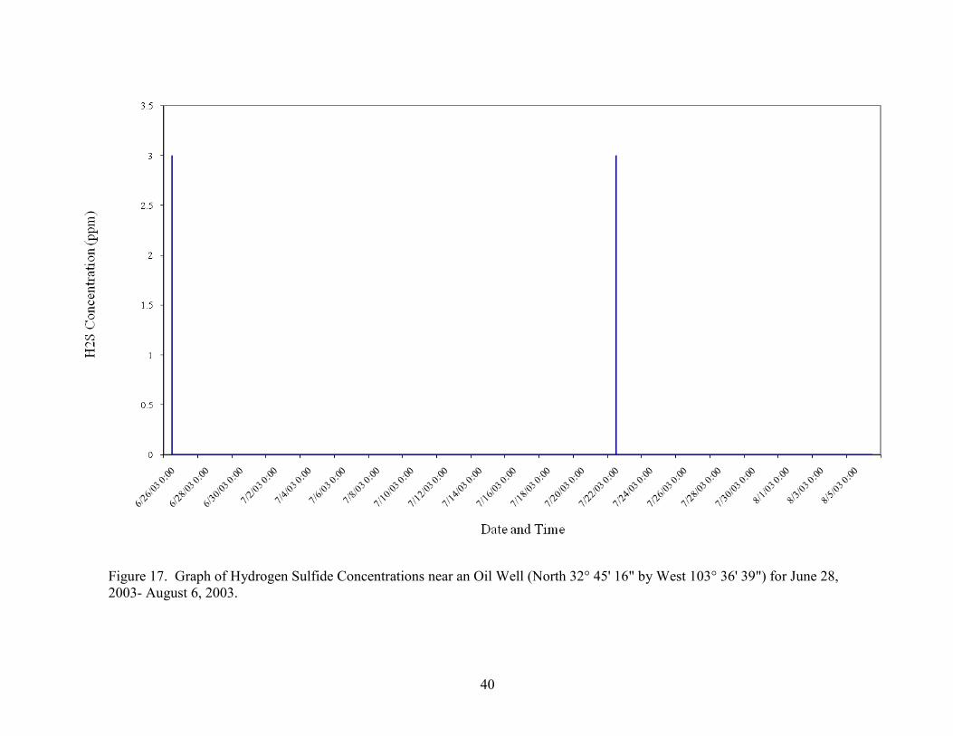
40
Figure 17. Graph of Hydrogen Sulfide Concentrations near an Oil Well (North 32° 45' 16" by West 103° 36' 39") for June 28, 2003- August 6, 2003.
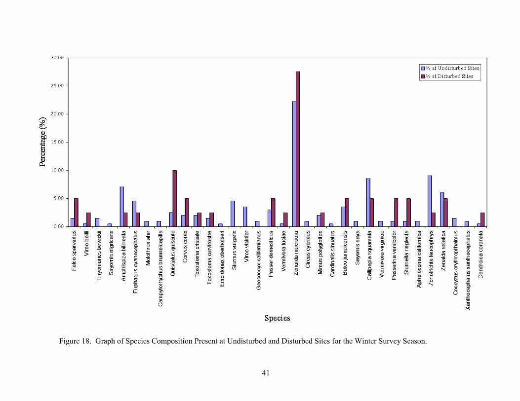
41
Figure 18. Graph of Species Composition Present at Undisturbed and Disturbed Sites for the Winter Survey Season.
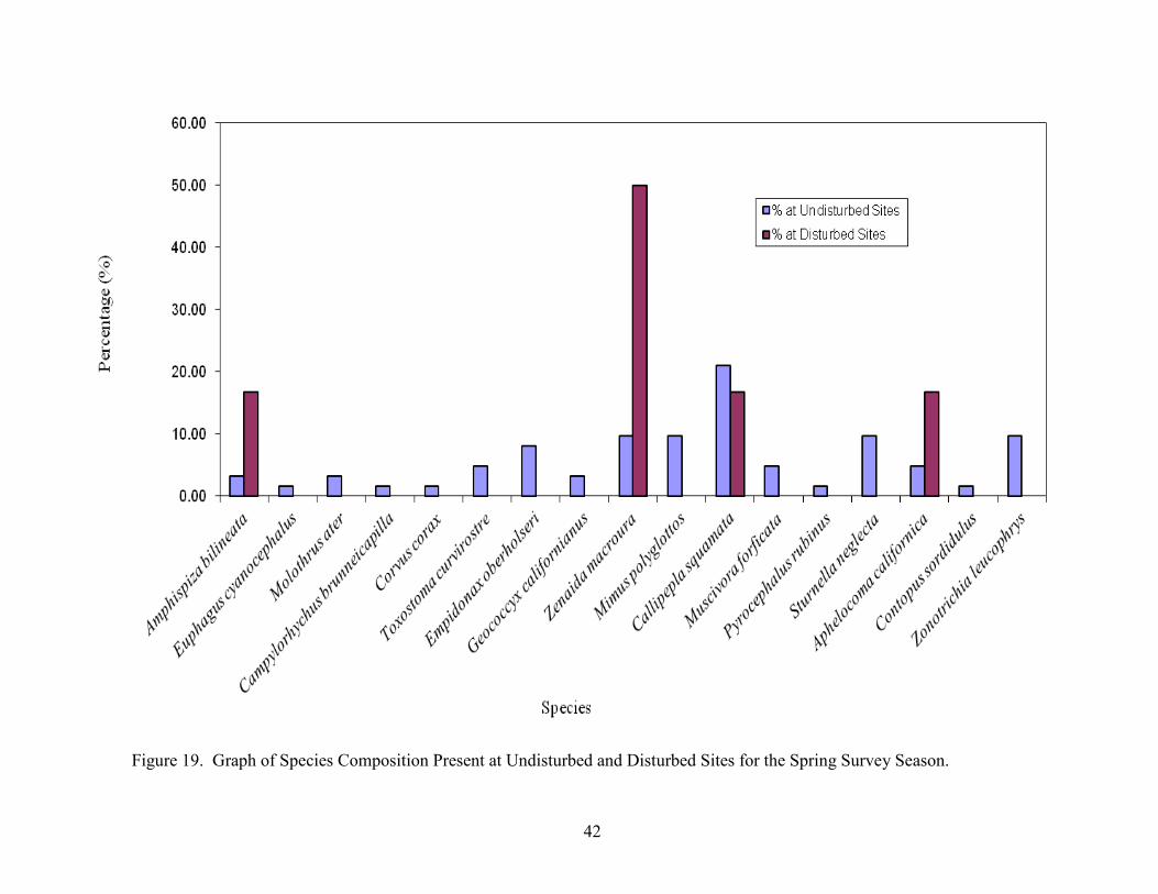
42
Figure 19. Graph of Species Composition Present at Undisturbed and Disturbed Sites for the Spring Survey Season.
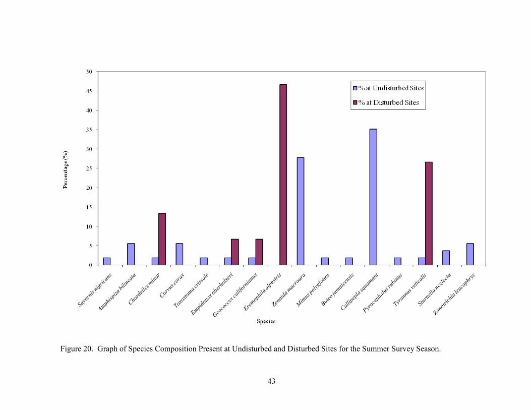
43
Figure 20. Graph of Species Composition Present at Undisturbed and Disturbed Sites for the Summer Survey Season.
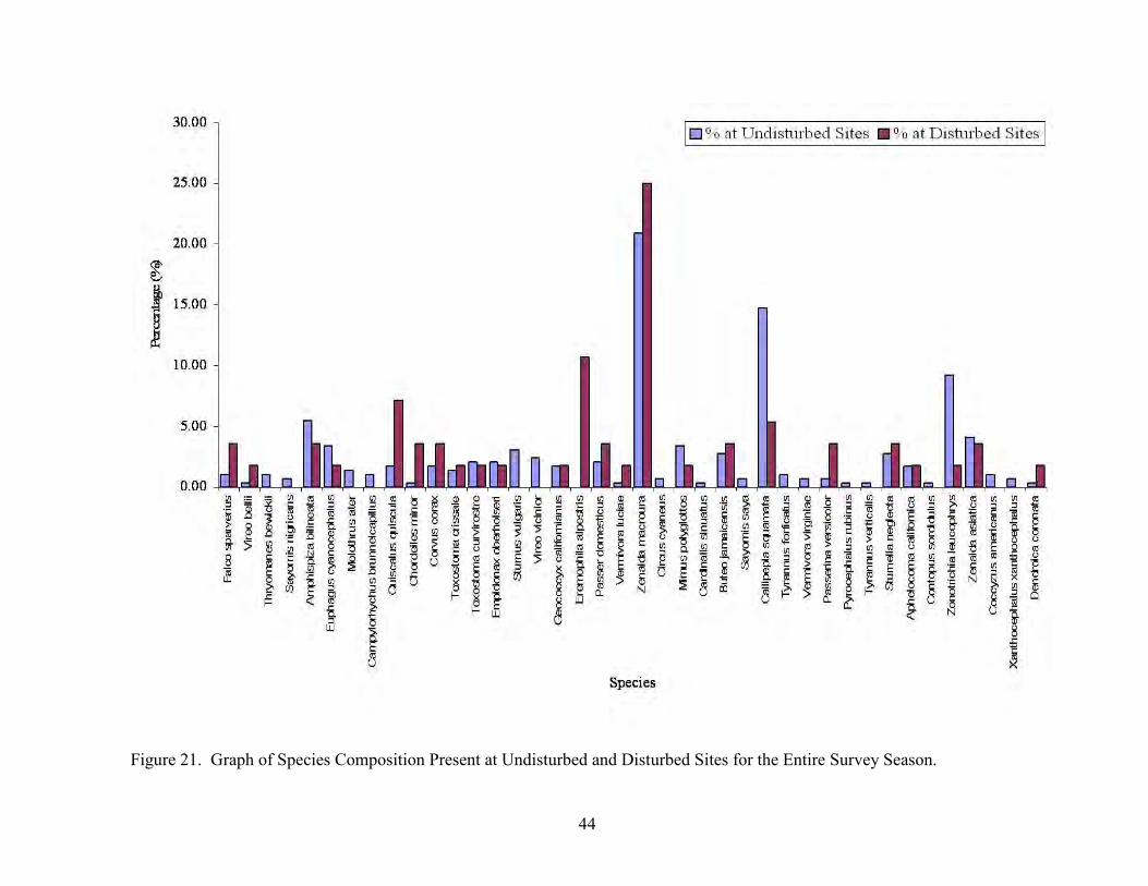
44
Figure 21. Graph of Species Composition Present at Undisturbed and Disturbed Sites for the Entire Survey Season.
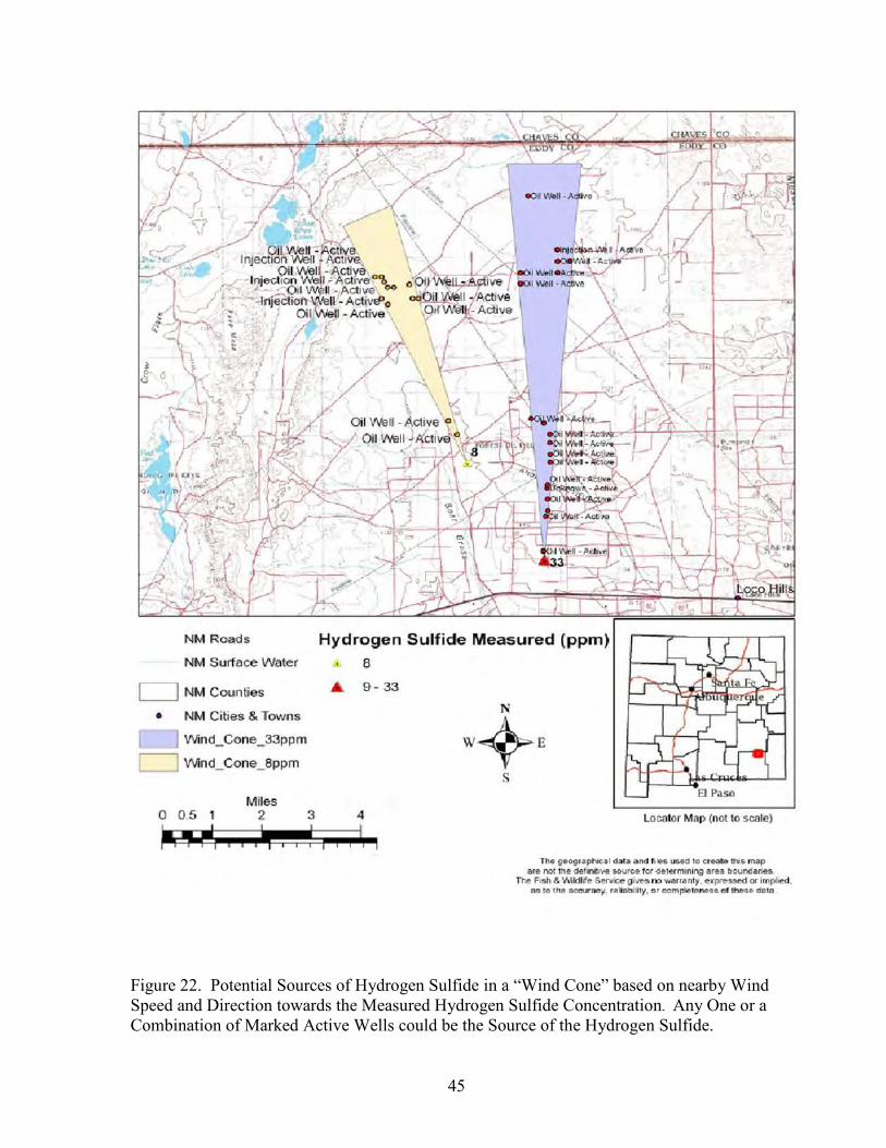
45
Figure 22. Potential Sources of Hydrogen Sulfide in a “Wind Cone” based on nearby Wind Speed and Direction towards the Measured Hydrogen Sulfide Concentration. Any One or a Combination of Marked Active Wells could be the Source of the Hydrogen Sulfide.
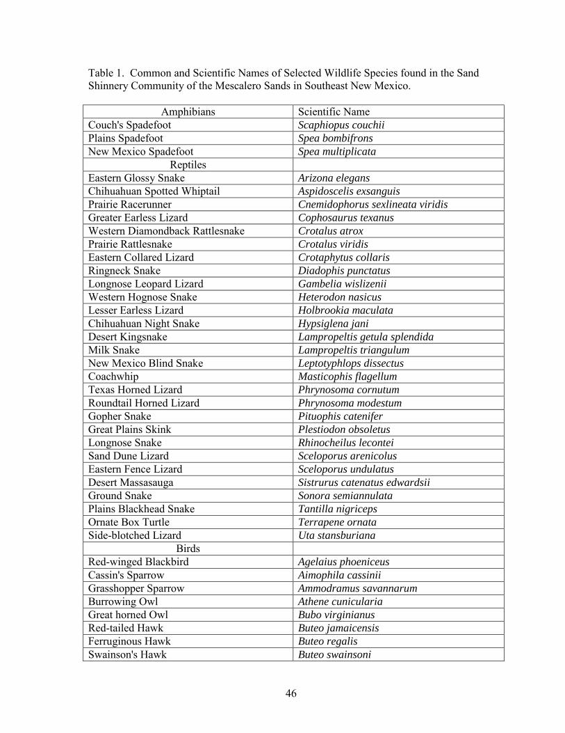
46
Table 1. Common and Scientific Names of Selected Wildlife Species found in the Sand Shinnery Community of the Mescalero Sands in Southeast New Mexico.
Amphibians Scientific Name Couch's Spadefoot Scaphiopus couchii Plains Spadefoot Spea bombifrons New Mexico Spadefoot Spea multiplicata
Reptiles Eastern Glossy Snake Arizona elegans Chihuahuan Spotted Whiptail Aspidoscelis exsanguis Prairie Racerunner Cnemidophorus sexlineata viridis Greater Earless Lizard Cophosaurus texanus Western Diamondback Rattlesnake Crotalus atrox Prairie Rattlesnake Crotalus viridis Eastern Collared Lizard Crotaphytus collaris Ringneck Snake Diadophis punctatus Longnose Leopard Lizard Gambelia wislizenii Western Hognose Snake Heterodon nasicus Lesser Earless Lizard Holbrookia maculata Chihuahuan Night Snake Hypsiglena jani Desert Kingsnake Lampropeltis getula splendida Milk Snake Lampropeltis triangulum New Mexico Blind Snake Leptotyphlops dissectus Coachwhip Masticophis flagellum Texas Horned Lizard Phrynosoma cornutum Roundtail Horned Lizard Phrynosoma modestum Gopher Snake Pituophis catenifer Great Plains Skink Plestiodon obsoletus Longnose Snake Rhinocheilus lecontei Sand Dune Lizard Sceloporus arenicolus Eastern Fence Lizard Sceloporus undulatus Desert Massasauga Sistrurus catenatus edwardsii Ground Snake Sonora semiannulata Plains Blackhead Snake Tantilla nigriceps Ornate Box Turtle Terrapene ornata Side-blotched Lizard Uta stansburiana
Birds Red-winged Blackbird Agelaius phoeniceus Cassin's Sparrow Aimophila cassinii Grasshopper Sparrow Ammodramus savannarum Burrowing Owl Athene cunicularia Great horned Owl Bubo virginianus Red-tailed Hawk Buteo jamaicensis Ferruginous Hawk Buteo regalis Swainson's Hawk Buteo swainsoni
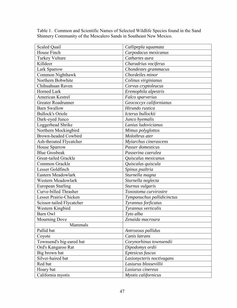
47
Table 1. Common and Scientific Names of Selected Wildlife Species found in the Sand Shinnery Community of the Mescalero Sands in Southeast New Mexico. Scaled Quail Callipepla squamata House Finch Carpodacus mexicanus Turkey Vulture Cathartes aura Killdeer Charadrius vociferus Lark Sparrow Chondestes grammacus Common Nighthawk Chordeiles minor Northern Bobwhite Colinus virginianus Chihuahuan Raven Corvus cryptoleucus Horned Lark Eremophila alpestris American Kestrel Falco sparverius Greater Roadrunner Geococcyx californianus Barn Swallow Hirundo rustica Bullock's Oriole Icterus bullockii Dark-eyed Junco Junco hyemalis Loggerhead Shrike Lanius ludovicianus Northern Mockingbird Mimus polyglottos Brown-headed Cowbird Molothrus ater Ash-throated Flycatcher Myiarchus cinerascens House Sparrow Passer domesticus Blue Grosbeak Passerina caerulea Great-tailed Grackle Quiscalus mexicanus Common Grackle Quiscalus quiscula Lesser Goldfinch Spinus psaltria Eastern Meadowlark Sturnella magna Western Meadowlark Sturnella neglecta European Starling Sturnus vulgaris Curve-billed Thrasher Toxostoma curvirostre Lesser Prairie-Chicken Tympanuchus pallidicinctus Scissor-tailed Flycatcher Tyrannus forficatus Western Kingbird Tyrannus verticalis Barn Owl Tyto alba Mourning Dove Zenaida macroura
Mammals Pallid bat Antrozous pallidus Coyote Canis latrans Townsend's big-eared bat Corynorhinus townsendii Ord's Kangaroo Rat Dipodomys ordii Big brown bat Eptesicus fuscus Silver-haired bat Lasionycteris noctivagans Red bat Lasiurus blossevillii Hoary bat Lasiurus cinereus California myotis Myotis californicus
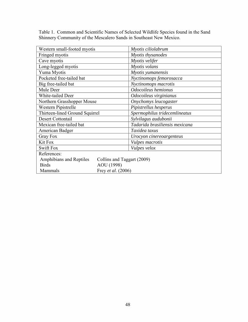
48
Table 1. Common and Scientific Names of Selected Wildlife Species found in the Sand Shinnery Community of the Mescalero Sands in Southeast New Mexico. Western small-footed myotis Myotis ciliolabrum Fringed myotis Myotis thysanodes Cave myotis Myotis velifer Long-legged myotis Myotis volans Yuma Myotis Myotis yumanensis Pocketed free-tailed bat Nyctinomops femorosacca Big free-tailed bat Nyctinomops macrotis Mule Deer Odocoileus hemionus White-tailed Deer Odocoileus virginianus Northern Grasshopper Mouse Onychomys leucogaster Western Pipistrelle Pipistrellus hesperus Thirteen-lined Ground Squirrel Spermophilus tridecemlineatus Desert Cottontail Sylvilagus audubonii Mexican free-tailed bat Tadarida brasiliensis mexicana American Badger Taxidea taxus Gray Fox Urocyon cinereoargenteus Kit Fox Vulpes macrotis Swift Fox Vulpes velox References: Amphibians and Reptiles Collins and Taggart (2009) Birds AOU (1998) Mammals Frey et al. (2006)
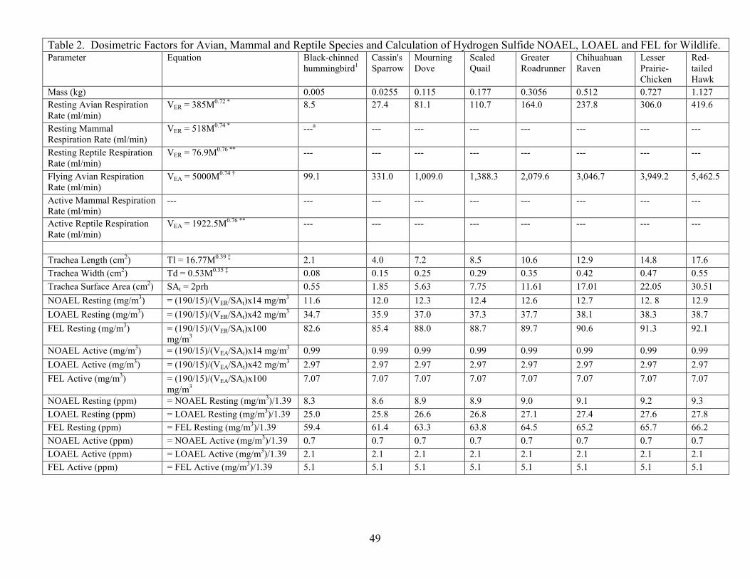
49
Table 2. Dosimetric Factors for Avian, Mammal and Reptile Species and Calculation of Hydrogen Sulfide NOAEL, LOAEL and FEL for Wildlife. Parameter Equation Black-chinned
hummingbird1 Cassin's Sparrow
Mourning Dove
Scaled Quail
Greater Roadrunner
Chihuahuan Raven
Lesser Prairie-Chicken
Red-tailed Hawk
Mass (kg) 0.005 0.0255 0.115 0.177 0.3056 0.512 0.727 1.127 Resting Avian Respiration Rate (ml/min)
VER = 385M0.72 * 8.5 27.4 81.1 110.7 164.0 237.8 306.0 419.6
Resting Mammal Respiration Rate (ml/min)
VER = 518M0.74 * ---a --- --- --- --- --- --- ---
Resting Reptile Respiration Rate (ml/min)
VER = 76.9M0.76 ** --- --- --- --- --- --- --- ---
Flying Avian Respiration Rate (ml/min)
VEA = 5000M0.74 † 99.1 331.0 1,009.0 1,388.3 2,079.6 3,046.7 3,949.2 5,462.5
Active Mammal Respiration Rate (ml/min)
--- --- --- --- --- --- --- --- ---
Active Reptile Respiration Rate (ml/min)
VEA = 1922.5M0.76 ** --- --- --- --- --- --- --- ---
Trachea Length (cm2) Tl = 16.77M0.39 ‡ 2.1 4.0 7.2 8.5 10.6 12.9 14.8 17.6 Trachea Width (cm2) Td = 0.53M0.35 ‡ 0.08 0.15 0.25 0.29 0.35 0.42 0.47 0.55 Trachea Surface Area (cm2) SAt = 2prh 0.55 1.85 5.63 7.75 11.61 17.01 22.05 30.51 NOAEL Resting (mg/m3) = (190/15)/(VER/SAt)x14 mg/m3 11.6 12.0 12.3 12.4 12.6 12.7 12. 8 12.9 LOAEL Resting (mg/m3) = (190/15)/(VER/SAt)x42 mg/m3 34.7 35.9 37.0 37.3 37.7 38.1 38.3 38.7 FEL Resting (mg/m3) = (190/15)/(VER/SAt)x100
mg/m3 82.6 85.4 88.0 88.7 89.7 90.6 91.3 92.1
NOAEL Active (mg/m3) = (190/15)/(VEA/SAt)x14 mg/m3 0.99 0.99 0.99 0.99 0.99 0.99 0.99 0.99 LOAEL Active (mg/m3) = (190/15)/(VEA/SAt)x42 mg/m3 2.97 2.97 2.97 2.97 2.97 2.97 2.97 2.97 FEL Active (mg/m3) = (190/15)/(VEA/SAt)x100
mg/m3 7.07 7.07 7.07 7.07 7.07 7.07 7.07 7.07
NOAEL Resting (ppm) = NOAEL Resting (mg/m3)/1.39 8.3 8.6 8.9 8.9 9.0 9.1 9.2 9.3 LOAEL Resting (ppm) = LOAEL Resting (mg/m3)/1.39 25.0 25.8 26.6 26.8 27.1 27.4 27.6 27.8 FEL Resting (ppm) = FEL Resting (mg/m3)/1.39 59.4 61.4 63.3 63.8 64.5 65.2 65.7 66.2 NOAEL Active (ppm) = NOAEL Active (mg/m3)/1.39 0.7 0.7 0.7 0.7 0.7 0.7 0.7 0.7 LOAEL Active (ppm) = LOAEL Active (mg/m3)/1.39 2.1 2.1 2.1 2.1 2.1 2.1 2.1 2.1 FEL Active (ppm) = FEL Active (mg/m3)/1.39 5.1 5.1 5.1 5.1 5.1 5.1 5.1 5.1
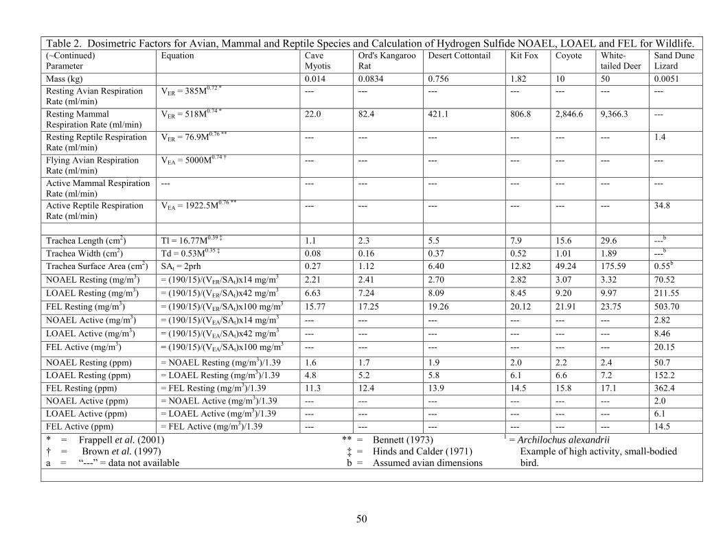
50
Table 2. Dosimetric Factors for Avian, Mammal and Reptile Species and Calculation of Hydrogen Sulfide NOAEL, LOAEL and FEL for Wildlife. (~Continued) Parameter
Equation Cave Myotis
Ord's Kangaroo Rat
Desert Cottontail Kit Fox Coyote White-tailed Deer
Sand Dune Lizard
Mass (kg) 0.014 0.0834 0.756 1.82 10 50 0.0051 Resting Avian Respiration Rate (ml/min)
VER = 385M0.72 * --- --- --- --- --- --- ---
Resting Mammal Respiration Rate (ml/min)
VER = 518M0.74 * 22.0 82.4 421.1 806.8 2,846.6 9,366.3 ---
Resting Reptile Respiration Rate (ml/min)
VER = 76.9M0.76 ** --- --- --- --- --- --- 1.4
Flying Avian Respiration Rate (ml/min)
VEA = 5000M0.74 † --- --- --- --- --- --- ---
Active Mammal Respiration Rate (ml/min)
--- --- --- --- --- --- --- ---
Active Reptile Respiration Rate (ml/min)
VEA = 1922.5M0.76 ** --- --- --- --- --- --- 34.8
Trachea Length (cm2) Tl = 16.77M0.39 ‡ 1.1 2.3 5.5 7.9 15.6 29.6 ---b Trachea Width (cm2) Td = 0.53M0.35 ‡ 0.08 0.16 0.37 0.52 1.01 1.89 ---b Trachea Surface Area (cm2) SAt = 2prh 0.27 1.12 6.40 12.82 49.24 175.59 0.55b NOAEL Resting (mg/m3) = (190/15)/(VER/SAt)x14 mg/m3 2.21 2.41 2.70 2.82 3.07 3.32 70.52 LOAEL Resting (mg/m3) = (190/15)/(VER/SAt)x42 mg/m3 6.63 7.24 8.09 8.45 9.20 9.97 211.55 FEL Resting (mg/m3) = (190/15)/(VER/SAt)x100 mg/m3 15.77 17.25 19.26 20.12 21.91 23.75 503.70 NOAEL Active (mg/m3) = (190/15)/(VEA/SAt)x14 mg/m3 --- --- --- --- --- --- 2.82 LOAEL Active (mg/m3) = (190/15)/(VEA/SAt)x42 mg/m3 --- --- --- --- --- --- 8.46 FEL Active (mg/m3) = (190/15)/(VEA/SAt)x100 mg/m3 --- --- --- --- --- --- 20.15
NOAEL Resting (ppm) = NOAEL Resting (mg/m3)/1.39 1.6 1.7 1.9 2.0 2.2 2.4 50.7 LOAEL Resting (ppm) = LOAEL Resting (mg/m3)/1.39 4.8 5.2 5.8 6.1 6.6 7.2 152.2 FEL Resting (ppm) = FEL Resting (mg/m3)/1.39 11.3 12.4 13.9 14.5 15.8 17.1 362.4 NOAEL Active (ppm) = NOAEL Active (mg/m3)/1.39 --- --- --- --- --- --- 2.0 LOAEL Active (ppm) = LOAEL Active (mg/m3)/1.39 --- --- --- --- --- --- 6.1 FEL Active (ppm) = FEL Active (mg/m3)/1.39 --- --- --- --- --- --- 14.5 * = Frappell et al. (2001) ** = Bennett (1973) 1 = Archilochus alexandrii † = Brown et al. (1997) ‡ = Hinds and Calder (1971) Example of high activity, small-bodied a = “---” = data not available b = Assumed avian dimensions bird.
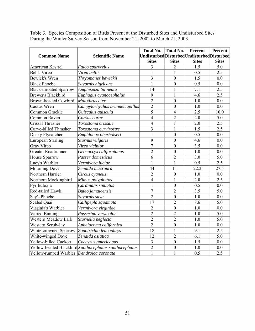
51
Table 3. Species Composition of Birds Present at the Disturbed Sites and Undisturbed Sites During the Winter Survey Season from November 21, 2002 to March 21, 2003.
Common Name Scientific Name Total No.
Undisturbed Sites
Total No. Disturbed
Sites
Percent Undisturbed
Sites
Percent Disturbed
Sites American Kestrel Falco sparverius 3 2 1.5 5.0 Bell's Vireo Vireo bellii 1 1 0.5 2.5 Bewick's Wren Thryomanes bewickii 3 0 1.5 0.0 Black Phoebe Sayornis nigricans 1 0 0.5 0.0 Black-throated Sparrow Amphispiza bilineata 14 1 7.1 2.5 Brewer's Blackbird Euphagus cyanocephalus 9 1 4.6 2.5 Brown-headed Cowbird Molothrus ater 2 0 1.0 0.0 Cactus Wren Campylorhychus brunneicapillus 2 0 1.0 0.0 Common Grackle Quiscalus quiscula 5 4 2.5 10.0 Common Raven Corvus corax 4 2 2.0 5.0 Crissal Thrasher Toxostoma crissale 4 1 2.0 2.5 Curve-billed Thrasher Toxostoma curvirostre 3 1 1.5 2.5 Dusky Flycatcher Empidonax oberholseri 1 0 0.5 0.0 European Starling Sturnus vulgaris 9 0 4.6 0.0 Gray Vireo Vireo vicinior 7 0 3.5 0.0 Greater Roadrunner Geococcyx californianus 2 0 1.0 0.0 House Sparrow Passer domesticus 6 2 3.0 5.0 Lucy's Warbler Vermivora luciae 1 1 0.5 2.5 Mourning Dove Zenaida macroura 44 11 22.2 27.5 Northern Harrier Circus cyaneus 2 0 1.0 0.0 Northern Mockingbird Mimus polyglottos 4 1 2.0 2.5 Pyrrhuloxia Cardinalis sinuatus 1 0 0.5 0.0 Red-tailed Hawk Buteo jamaicensis 7 2 3.5 5.0 Say's Phoebe Sayornis saya 2 0 1.0 0.0 Scaled Quail Callipepla squamata 17 2 8.6 5.0 Virginia's Warbler Vermivora virginiae 2 0 1.0 0.0 Varied Bunting Passerina versicolor 2 2 1.0 5.0 Western Meadow Lark Sturnella neglecta 2 2 1.0 5.0 Western Scrub-Jay Aphelocoma californica 2 0 1.0 0.0 White-crowned Sparrow Zonotrichia leucophrys 18 1 9.1 2.5 White-winged Dove Zenaida asiatica 12 2 6.1 5.0 Yellow-billed Cuckoo Coccyzus americanus 3 0 1.5 0.0 Yellow-headed Blackbird Xanthocephalus xanthocephalus 2 0 1.0 0.0 Yellow-rumped Warbler Dendroica coronata 1 1 0.5 2.5
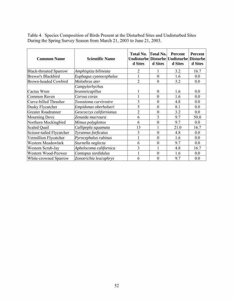
52
Table 4. Species Composition of Birds Present at the Disturbed Sites and Undisturbed Sites During the Spring Survey Season from March 21, 2003 to June 21, 2003.
Common Name Scientific Name Total No.
Undisturbed Sites
Total No. Disturbed Sites
Percent Undisturbe
d Sites
Percent Disturbed Sites
Black-throated Sparrow Amphispiza bilineata 2 1 3.2 16.7 Brewer's Blackbird Euphagus cyanocephalus 1 0 1.6 0.0 Brown-headed Cowbird Molothrus ater 2 0 3.2 0.0
Cactus Wren Campylorhychus brunneicapillus 1 0 1.6 0.0
Common Raven Corvus corax 1 0 1.6 0.0 Curve-billed Thrasher Toxostoma curvirostre 3 0 4.8 0.0 Dusky Flycatcher Empidonax oberholseri 5 0 8.1 0.0 Greater Roadrunner Geococcyx californianus 2 0 3.2 0.0 Mourning Dove Zenaida macroura 6 3 9.7 50.0 Northern Mockingbird Mimus polyglottos 6 0 9.7 0.0 Scaled Quail Callipepla squamata 13 1 21.0 16.7 Scissor-tailed Flycatcher Tyrannus forficatus 3 0 4.8 0.0 Vermillion Flycatcher Pyrocephalus rubinus 1 0 1.6 0.0 Western Meadowlark Sturnella neglecta 6 0 9.7 0.0 Western Scrub-Jay Aphelocoma californica 3 1 4.8 16.7 Western Wood-Peewee Contopus sordidulus 1 0 1.6 0.0 White-crowned Sparrow Zonotrichia leucophrys 6 0 9.7 0.0
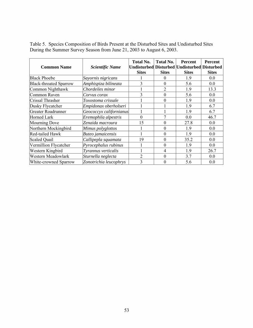
53
Table 5. Species Composition of Birds Present at the Disturbed Sites and Undisturbed Sites During the Summer Survey Season from June 21, 2003 to August 6, 2003.
Common Name Scientific Name Total No.
Undisturbed Sites
Total No. Disturbed
Sites
Percent Undisturbed
Sites
Percent Disturbed
Sites Black Phoebe Sayornis nigricans 1 0 1.9 0.0 Black-throated Sparrow Amphispiza bilineata 3 0 5.6 0.0 Common Nighthawk Chordeiles minor 1 2 1.9 13.3 Common Raven Corvus corax 3 0 5.6 0.0 Crissal Thrasher Toxostoma crissale 1 0 1.9 0.0 Dusky Flycatcher Empidonax oberholseri 1 1 1.9 6.7 Greater Roadrunner Geococcyx californianus 1 1 1.9 6.7 Horned Lark Eremophila alpestris 0 7 0.0 46.7 Mourning Dove Zenaida macroura 15 0 27.8 0.0 Northern Mockingbird Mimus polyglottos 1 0 1.9 0.0 Red-tailed Hawk Buteo jamaicensis 1 0 1.9 0.0 Scaled Quail Callipepla squamata 19 0 35.2 0.0 Vermillion Flycatcher Pyrocephalus rubinus 1 0 1.9 0.0 Western Kingbird Tyrannus verticalis 1 4 1.9 26.7 Western Meadowlark Sturnella neglecta 2 0 3.7 0.0 White-crowned Sparrow Zonotrichia leucophrys 3 0 5.6 0.0
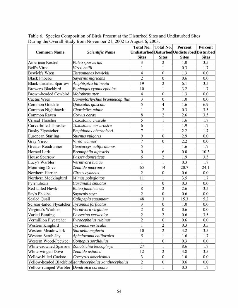
54
Table 6. Species Composition of Birds Present at the Disturbed Sites and Undisturbed Sites During the Overall Study from November 21, 2002 to August 6, 2003.
Common Name Scientific Name Total No.
Undisturbed Sites
Total No. Disturbed
Sites
Percent Undisturbed
Sites
Percent Disturbed
Sites American Kestrel Falco sparverius 3 2 1.0 3.5 Bell's Vireo Vireo bellii 1 1 0.3 1.7 Bewick's Wren Thryomanes bewickii 4 0 1.3 0.0 Black Phoebe Sayornis nigricans 2 0 0.6 0.0 Black-throated Sparrow Amphispiza bilineata 19 2 6.1 3.5 Brewer's Blackbird Euphagus cyanocephalus 10 1 3.2 1.7 Brown-headed Cowbird Molothrus ater 4 0 1.3 0.0 Cactus Wren Campylorhychus brunneicapillus 3 0 1.0 0.0 Common Grackle Quiscalus quiscula 5 4 1.6 6.9 Common Nighthawk Chordeiles minor 1 2 0.3 3.5 Common Raven Corvus corax 8 2 2.6 3.5 Crissal Thrasher Toxostoma crissale 5 1 1.6 1.7 Curve-billed Thrasher Toxostoma curvirostre 6 1 1.9 1.7 Dusky Flycatcher Empidonax oberholseri 7 1 2.2 1.7 European Starling Sturnus vulgaris 9 0 2.9 0.0 Gray Vireo Vireo vicinior 7 0 2.2 0.0 Greater Roadrunner Geococcyx californianus 5 1 1.6 1.7 Horned Lark Eremophila alpestris 0 6 0.0 10.3 House Sparrow Passer domesticus 6 2 1.9 3.5 Lucy's Warbler Vermivora luciae 1 1 0.3 1.7 Mourning Dove Zenaida macroura 65 14 20.7 24.1 Northern Harrier Circus cyaneus 2 0 0.6 0.0 Northern Mockingbird Mimus polyglottos 11 1 3.5 1.7 Pyrrhuloxia Cardinalis sinuatus 1 0 0.3 0.0 Red-tailed Hawk Buteo jamaicensis 8 2 2.6 3.5 Say's Phoebe Sayornis saya 2 0 0.6 0.0 Scaled Quail Callipepla squamata 48 3 15.3 5.2 Scissor-tailed Flycatcher Tyrannus forficatus 3 0 1.0 0.0 Virginia's Warbler Vermivora virginiae 2 0 0.6 0.0 Varied Bunting Passerina versicolor 2 2 0.6 3.5 Vermillion Flycatcher Pyrocephalus rubinus 2 0 0.6 0.0 Western Kingbird Tyrannus verticalis 1 2 0.3 3.5 Western Meadowlark Sturnella neglecta 10 2 3.2 3.5 Western Scrub-Jay Aphelocoma californica 5 1 1.6 1.7 Western Wood-Peewee Contopus sordidulus 1 0 0.3 0.0 White-crowned Sparrow Zonotrichia leucophrys 27 1 8.6 1.7 White-winged Dove Zenaida asiatica 12 2 3.8 3.5 Yellow-billed Cuckoo Coccyzus americanus 3 0 1.0 0.0 Yellow-headed Blackbird Xanthocephalus xanthocephalus 2 0 0.6 0.0 Yellow-rumped Warbler Dendroica coronata 1 1 0.3 1.7
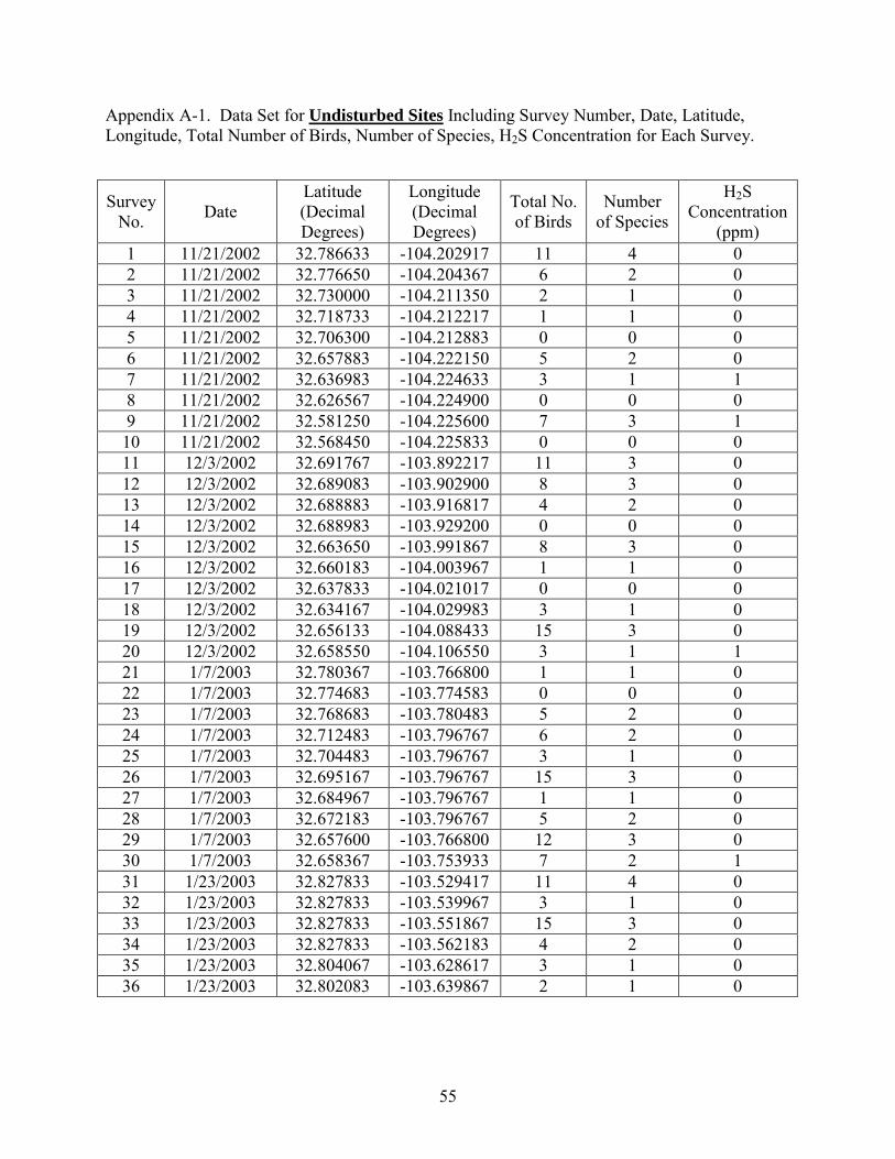
55
Appendix A-1. Data Set for Undisturbed Sites Including Survey Number, Date, Latitude, Longitude, Total Number of Birds, Number of Species, H2S Concentration for Each Survey.
Survey No. Date
Latitude (Decimal Degrees)
Longitude (Decimal Degrees)
Total No. of Birds
Number of Species
H2S Concentration
(ppm) 1 11/21/2002 32.786633 -104.202917 11 4 0 2 11/21/2002 32.776650 -104.204367 6 2 0 3 11/21/2002 32.730000 -104.211350 2 1 0 4 11/21/2002 32.718733 -104.212217 1 1 0 5 11/21/2002 32.706300 -104.212883 0 0 0 6 11/21/2002 32.657883 -104.222150 5 2 0 7 11/21/2002 32.636983 -104.224633 3 1 1 8 11/21/2002 32.626567 -104.224900 0 0 0 9 11/21/2002 32.581250 -104.225600 7 3 1 10 11/21/2002 32.568450 -104.225833 0 0 0 11 12/3/2002 32.691767 -103.892217 11 3 0 12 12/3/2002 32.689083 -103.902900 8 3 0 13 12/3/2002 32.688883 -103.916817 4 2 0 14 12/3/2002 32.688983 -103.929200 0 0 0 15 12/3/2002 32.663650 -103.991867 8 3 0 16 12/3/2002 32.660183 -104.003967 1 1 0 17 12/3/2002 32.637833 -104.021017 0 0 0 18 12/3/2002 32.634167 -104.029983 3 1 0 19 12/3/2002 32.656133 -104.088433 15 3 0 20 12/3/2002 32.658550 -104.106550 3 1 1 21 1/7/2003 32.780367 -103.766800 1 1 0 22 1/7/2003 32.774683 -103.774583 0 0 0 23 1/7/2003 32.768683 -103.780483 5 2 0 24 1/7/2003 32.712483 -103.796767 6 2 0 25 1/7/2003 32.704483 -103.796767 3 1 0 26 1/7/2003 32.695167 -103.796767 15 3 0 27 1/7/2003 32.684967 -103.796767 1 1 0 28 1/7/2003 32.672183 -103.796767 5 2 0 29 1/7/2003 32.657600 -103.766800 12 3 0 30 1/7/2003 32.658367 -103.753933 7 2 1 31 1/23/2003 32.827833 -103.529417 11 4 0 32 1/23/2003 32.827833 -103.539967 3 1 0 33 1/23/2003 32.827833 -103.551867 15 3 0 34 1/23/2003 32.827833 -103.562183 4 2 0 35 1/23/2003 32.804067 -103.628617 3 1 0 36 1/23/2003 32.802083 -103.639867 2 1 0
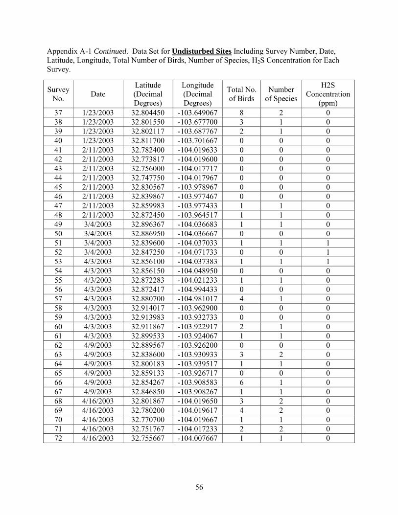
56
Appendix A-1 Continued. Data Set for Undisturbed Sites Including Survey Number, Date, Latitude, Longitude, Total Number of Birds, Number of Species, H2S Concentration for Each Survey.
Survey No. Date
Latitude (Decimal Degrees)
Longitude (Decimal Degrees)
Total No. of Birds
Number of Species
H2S Concentration
(ppm) 37 1/23/2003 32.804450 -103.649067 8 2 0 38 1/23/2003 32.801550 -103.677700 3 1 0 39 1/23/2003 32.802117 -103.687767 2 1 0 40 1/23/2003 32.811700 -103.701667 0 0 0 41 2/11/2003 32.782400 -104.019633 0 0 0 42 2/11/2003 32.773817 -104.019600 0 0 0 43 2/11/2003 32.756000 -104.017717 0 0 0 44 2/11/2003 32.747750 -104.017967 0 0 0 45 2/11/2003 32.830567 -103.978967 0 0 0 46 2/11/2003 32.839867 -103.977467 0 0 0 47 2/11/2003 32.859983 -103.977433 1 1 0 48 2/11/2003 32.872450 -103.964517 1 1 0 49 3/4/2003 32.896367 -104.036683 1 1 0 50 3/4/2003 32.886950 -104.036667 0 0 0 51 3/4/2003 32.839600 -104.037033 1 1 1 52 3/4/2003 32.847250 -104.071733 0 0 1 53 4/3/2003 32.856100 -104.037383 1 1 1 54 4/3/2003 32.856150 -104.048950 0 0 0 55 4/3/2003 32.872283 -104.021233 1 1 0 56 4/3/2003 32.872417 -104.994433 0 0 0 57 4/3/2003 32.880700 -104.981017 4 1 0 58 4/3/2003 32.914017 -103.962900 0 0 0 59 4/3/2003 32.913983 -103.932733 0 0 0 60 4/3/2003 32.911867 -103.922917 2 1 0 61 4/3/2003 32.899533 -103.924067 1 1 0 62 4/9/2003 32.889567 -103.926200 0 0 0 63 4/9/2003 32.838600 -103.930933 3 2 0 64 4/9/2003 32.800183 -103.939517 1 1 0 65 4/9/2003 32.859133 -103.926717 0 0 0 66 4/9/2003 32.854267 -103.908583 6 1 0 67 4/9/2003 32.846850 -103.908267 1 1 0 68 4/16/2003 32.801867 -104.019650 3 2 0 69 4/16/2003 32.780200 -104.019617 4 2 0 70 4/16/2003 32.770700 -104.019667 1 1 0 71 4/16/2003 32.751767 -104.017233 2 2 0 72 4/16/2003 32.755667 -104.007667 1 1 0
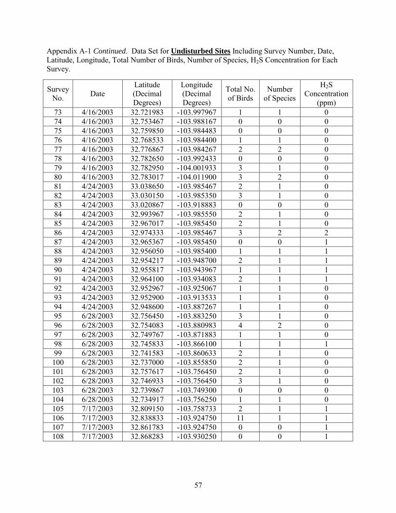
57
Appendix A-1 Continued. Data Set for Undisturbed Sites Including Survey Number, Date, Latitude, Longitude, Total Number of Birds, Number of Species, H2S Concentration for Each Survey.
Survey No. Date
Latitude (Decimal Degrees)
Longitude (Decimal Degrees)
Total No. of Birds
Number of Species
H2S Concentration
(ppm) 73 4/16/2003 32.721983 -103.997967 1 1 0 74 4/16/2003 32.753467 -103.988167 0 0 0 75 4/16/2003 32.759850 -103.984483 0 0 0 76 4/16/2003 32.768533 -103.984400 1 1 0 77 4/16/2003 32.776867 -103.984267 2 2 0 78 4/16/2003 32.782650 -103.992433 0 0 0 79 4/16/2003 32.782950 -104.001933 3 1 0 80 4/16/2003 32.783017 -104.011900 3 2 0 81 4/24/2003 33.038650 -103.985467 2 1 0 82 4/24/2003 33.030150 -103.985350 3 1 0 83 4/24/2003 33.020867 -103.918883 0 0 0 84 4/24/2003 32.993967 -103.985550 2 1 0 85 4/24/2003 32.967017 -103.985450 2 1 0 86 4/24/2003 32.974333 -103.985467 3 2 2 87 4/24/2003 32.965367 -103.985450 0 0 1 88 4/24/2003 32.956050 -103.985400 1 1 1 89 4/24/2003 32.954217 -103.948700 2 1 1 90 4/24/2003 32.955817 -103.943967 1 1 1 91 4/24/2003 32.964100 -103.934083 2 1 1 92 4/24/2003 32.952967 -103.925067 1 1 0 93 4/24/2003 32.952900 -103.913533 1 1 0 94 4/24/2003 32.948600 -103.887267 1 1 0 95 6/28/2003 32.756450 -103.883250 3 1 0 96 6/28/2003 32.754083 -103.880983 4 2 0 97 6/28/2003 32.749767 -103.871883 1 1 0 98 6/28/2003 32.745833 -103.866100 1 1 1 99 6/28/2003 32.741583 -103.860633 2 1 0 100 6/28/2003 32.737000 -103.855850 2 1 0 101 6/28/2003 32.757617 -103.756450 2 1 0 102 6/28/2003 32.746933 -103.756450 3 1 0 103 6/28/2003 32.739867 -103.749300 0 0 0 104 6/28/2003 32.734917 -103.756250 1 1 0 105 7/17/2003 32.809150 -103.758733 2 1 1 106 7/17/2003 32.838833 -103.924750 11 1 1 107 7/17/2003 32.861783 -103.924750 0 0 1 108 7/17/2003 32.868283 -103.930250 0 0 1
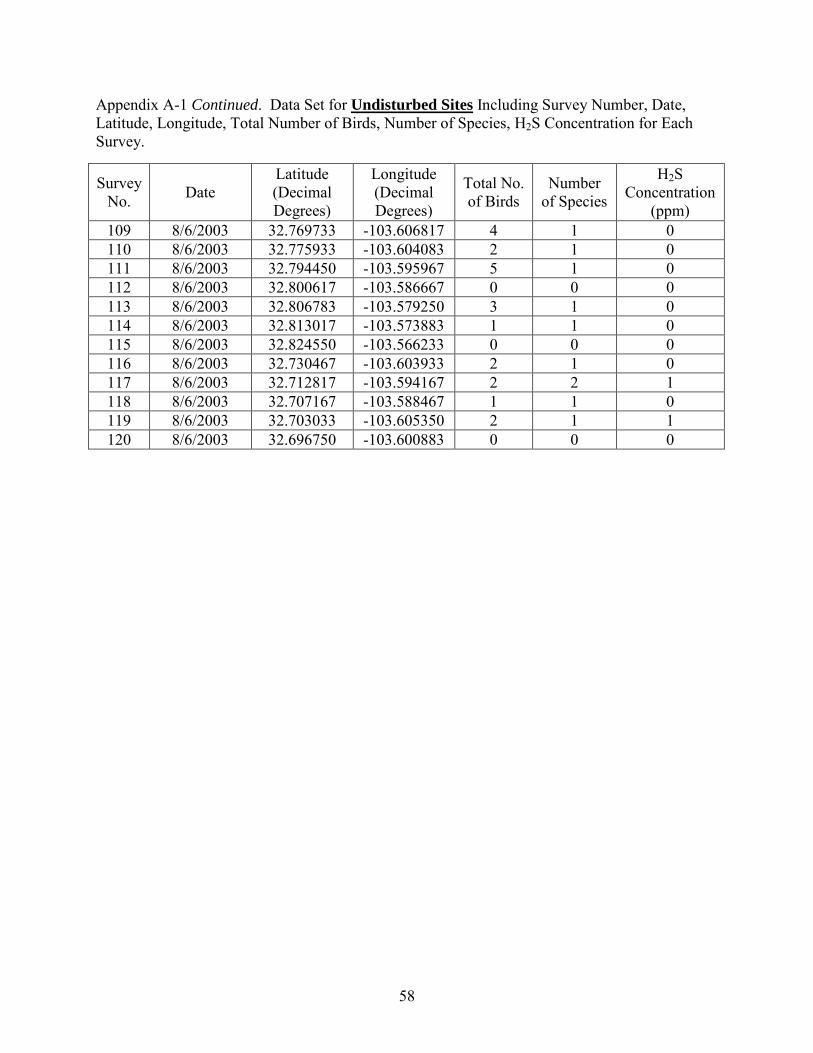
58
Appendix A-1 Continued. Data Set for Undisturbed Sites Including Survey Number, Date, Latitude, Longitude, Total Number of Birds, Number of Species, H2S Concentration for Each Survey.
Survey No. Date
Latitude (Decimal Degrees)
Longitude (Decimal Degrees)
Total No. of Birds
Number of Species
H2S Concentration
(ppm) 109 8/6/2003 32.769733 -103.606817 4 1 0 110 8/6/2003 32.775933 -103.604083 2 1 0 111 8/6/2003 32.794450 -103.595967 5 1 0 112 8/6/2003 32.800617 -103.586667 0 0 0 113 8/6/2003 32.806783 -103.579250 3 1 0 114 8/6/2003 32.813017 -103.573883 1 1 0 115 8/6/2003 32.824550 -103.566233 0 0 0 116 8/6/2003 32.730467 -103.603933 2 1 0 117 8/6/2003 32.712817 -103.594167 2 2 1 118 8/6/2003 32.707167 -103.588467 1 1 0 119 8/6/2003 32.703033 -103.605350 2 1 1 120 8/6/2003 32.696750 -103.600883 0 0 0

59
Appendix A-2. Data Set for Disturbed Sites Including Survey Number, Date, Latitude, Longitude, Total Number of Birds, Number of Species, H2S Concentration for Each Survey.
Survey No. Date
Latitude (Decimal Degrees)
Longitude (Decimal Degrees)
Total No. of Birds
Number of Species
H2S Concentration
(ppm) 1 11/21/2002 32.764950 -104.207317 2 1 1 2 11/21/2002 32.753683 -104.209450 0 0 1 3 11/21/2002 32.741717 -104.210450 0 0 1 4 11/21/2002 32.695083 -104.213800 0 0 1 5 11/21/2002 32.682267 -104.214250 3 2 1 6 11/21/2002 32.670817 -104.219483 1 1 2 7 11/21/2002 32.646967 -104.223650 1 1 2 8 11/21/2002 32.615283 -104.225183 4 2 2 9 11/21/2002 32.605017 -104.225917 0 0 1 10 11/21/2002 32.592950 -104.225383 0 0 1 11 12/3/2002 32.693867 -103.941650 0 0 1 12 12/3/2002 32.697467 -103.949500 2 1 1 13 12/3/2002 32.686917 -103.956583 1 1 2 14 12/3/2002 32.678967 -103.967950 1 1 2 15 12/3/2002 32.671317 -103.982783 1 1 2 16 12/3/2002 32.657633 -104.017700 0 0 2 17 12/3/2002 32.647167 -104.021617 0 0 1 18 12/3/2002 32.640000 -104.042883 2 2 2 19 12/3/2002 32.645200 -104.055767 0 0 1 20 12/3/2002 32.650883 -104.069900 0 0 2 21 1/7/2003 32.758133 -103.780633 0 0 3 22 1/7/2003 32.750250 -103.786133 2 1 1 23 1/7/2003 32.744567 -103.792800 0 0 1 24 1/7/2003 32.735500 -103.795700 2 1 1 25 1/7/2003 32.725517 -10.795517 4 2 1 26 1/7/2003 32.661983 -103.796633 0 0 1 27 1/7/2003 32.653433 -103.796417 2 1 1 28 1/7/2003 32.644850 -103.796417 3 3 2 29 1/7/2003 32.634467 -103.798033 0 0 2 30 1/7/2003 32.656950 -103.777617 0 0 2 31 1/23/2003 32.827050 -103.575317 0 0 2 32 1/23/2003 32.822850 -103.585217 2 1 1 33 1/23/2003 32.819467 -103.593400 0 0 1 34 1/23/2003 32.815533 -103.602667 0 0 1 35 1/23/2003 32.811417 -103.611967 1 1 1 36 1/23/2003 32.807950 -103.619833 2 1 3
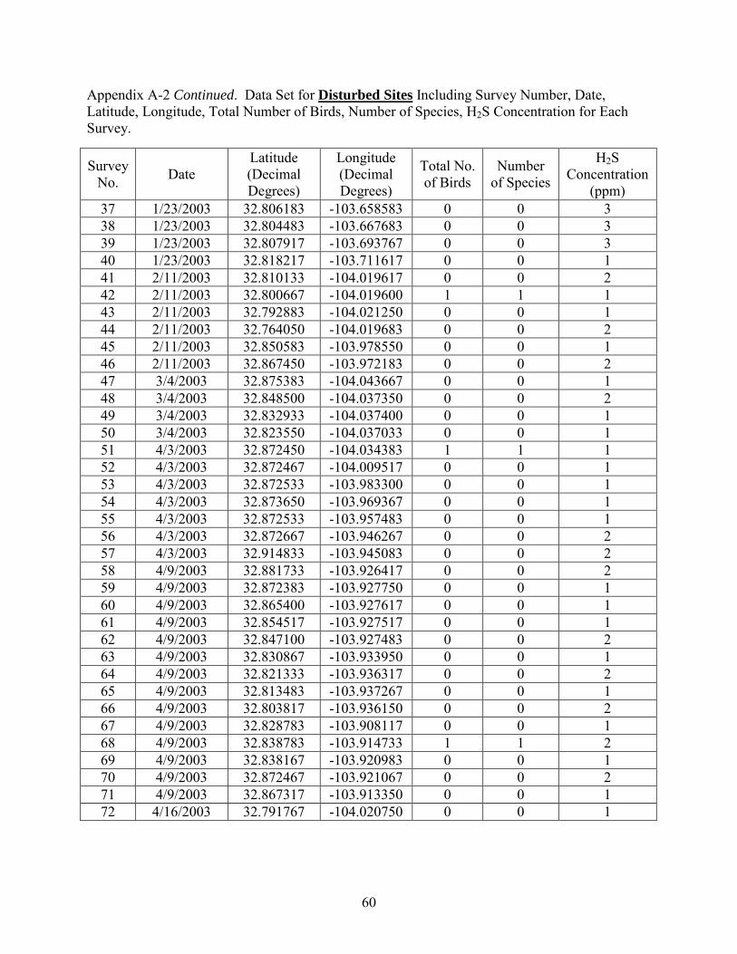
60
Appendix A-2 Continued. Data Set for Disturbed Sites Including Survey Number, Date, Latitude, Longitude, Total Number of Birds, Number of Species, H2S Concentration for Each Survey.
Survey No. Date
Latitude (Decimal Degrees)
Longitude (Decimal Degrees)
Total No. of Birds
Number of Species
H2S Concentration
(ppm) 37 1/23/2003 32.806183 -103.658583 0 0 3 38 1/23/2003 32.804483 -103.667683 0 0 3 39 1/23/2003 32.807917 -103.693767 0 0 3 40 1/23/2003 32.818217 -103.711617 0 0 1 41 2/11/2003 32.810133 -104.019617 0 0 2 42 2/11/2003 32.800667 -104.019600 1 1 1 43 2/11/2003 32.792883 -104.021250 0 0 1 44 2/11/2003 32.764050 -104.019683 0 0 2 45 2/11/2003 32.850583 -103.978550 0 0 1 46 2/11/2003 32.867450 -103.972183 0 0 2 47 3/4/2003 32.875383 -104.043667 0 0 1 48 3/4/2003 32.848500 -104.037350 0 0 2 49 3/4/2003 32.832933 -104.037400 0 0 1 50 3/4/2003 32.823550 -104.037033 0 0 1 51 4/3/2003 32.872450 -104.034383 1 1 1 52 4/3/2003 32.872467 -104.009517 0 0 1 53 4/3/2003 32.872533 -103.983300 0 0 1 54 4/3/2003 32.873650 -103.969367 0 0 1 55 4/3/2003 32.872533 -103.957483 0 0 1 56 4/3/2003 32.872667 -103.946267 0 0 2 57 4/3/2003 32.914833 -103.945083 0 0 2 58 4/9/2003 32.881733 -103.926417 0 0 2 59 4/9/2003 32.872383 -103.927750 0 0 1 60 4/9/2003 32.865400 -103.927617 0 0 1 61 4/9/2003 32.854517 -103.927517 0 0 1 62 4/9/2003 32.847100 -103.927483 0 0 2 63 4/9/2003 32.830867 -103.933950 0 0 1 64 4/9/2003 32.821333 -103.936317 0 0 2 65 4/9/2003 32.813483 -103.937267 0 0 1 66 4/9/2003 32.803817 -103.936150 0 0 2 67 4/9/2003 32.828783 -103.908117 0 0 1 68 4/9/2003 32.838783 -103.914733 1 1 2 69 4/9/2003 32.838167 -103.920983 0 0 1 70 4/9/2003 32.872467 -103.921067 0 0 2 71 4/9/2003 32.867317 -103.913350 0 0 1 72 4/16/2003 32.791767 -104.020750 0 0 1
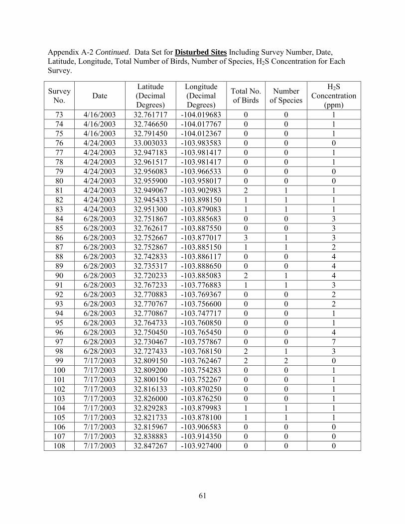
61
Appendix A-2 Continued. Data Set for Disturbed Sites Including Survey Number, Date, Latitude, Longitude, Total Number of Birds, Number of Species, H2S Concentration for Each Survey.
Survey No. Date
Latitude (Decimal Degrees)
Longitude (Decimal Degrees)
Total No. of Birds
Number of Species
H2S Concentration
(ppm) 73 4/16/2003 32.761717 -104.019683 0 0 1 74 4/16/2003 32.746650 -104.017767 0 0 1 75 4/16/2003 32.791450 -104.012367 0 0 1 76 4/24/2003 33.003033 -103.983583 0 0 0 77 4/24/2003 32.947183 -103.981417 0 0 1 78 4/24/2003 32.961517 -103.981417 0 0 1 79 4/24/2003 32.956083 -103.966533 0 0 0 80 4/24/2003 32.955900 -103.958017 0 0 0 81 4/24/2003 32.949067 -103.902983 2 1 1 82 4/24/2003 32.945433 -103.898150 1 1 1 83 4/24/2003 32.951300 -103.879083 1 1 1 84 6/28/2003 32.751867 -103.885683 0 0 3 85 6/28/2003 32.762617 -103.887550 0 0 3 86 6/28/2003 32.752667 -103.877017 3 1 3 87 6/28/2003 32.752867 -103.885150 1 1 2 88 6/28/2003 32.742833 -103.886117 0 0 4 89 6/28/2003 32.735317 -103.888650 0 0 4 90 6/28/2003 32.720233 -103.885083 2 1 4 91 6/28/2003 32.767233 -103.776883 1 1 3 92 6/28/2003 32.770883 -103.769367 0 0 2 93 6/28/2003 32.770767 -103.756600 0 0 2 94 6/28/2003 32.770867 -103.747717 0 0 1 95 6/28/2003 32.764733 -103.760850 0 0 1 96 6/28/2003 32.750450 -103.765450 0 0 4 97 6/28/2003 32.730467 -103.757867 0 0 7 98 6/28/2003 32.727433 -103.768150 2 1 3 99 7/17/2003 32.809150 -103.762467 2 2 0 100 7/17/2003 32.809200 -103.754283 0 0 1 101 7/17/2003 32.800150 -103.752267 0 0 1 102 7/17/2003 32.816133 -103.870250 0 0 1 103 7/17/2003 32.826000 -103.876250 0 0 1 104 7/17/2003 32.829283 -103.879983 1 1 1 105 7/17/2003 32.821733 -103.878100 1 1 1 106 7/17/2003 32.815967 -103.906583 0 0 0 107 7/17/2003 32.838883 -103.914350 0 0 0 108 7/17/2003 32.847267 -103.927400 0 0 0
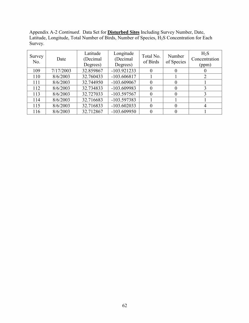
62
Appendix A-2 Continued. Data Set for Disturbed Sites Including Survey Number, Date, Latitude, Longitude, Total Number of Birds, Number of Species, H2S Concentration for Each Survey.
Survey No. Date
Latitude (Decimal Degrees)
Longitude (Decimal Degrees)
Total No. of Birds
Number of Species
H2S Concentration
(ppm) 109 7/17/2003 32.859867 -103.921233 0 0 0 110 8/6/2003 32.760433 -103.606817 1 1 2 111 8/6/2003 32.744950 -103.609067 0 0 1 112 8/6/2003 32.734833 -103.609983 0 0 3 113 8/6/2003 32.727033 -103.597567 0 0 3 114 8/6/2003 32.716683 -103.597383 1 1 1 115 8/6/2003 32.716833 -103.602033 0 0 4 116 8/6/2003 32.712867 -103.609950 0 0 1
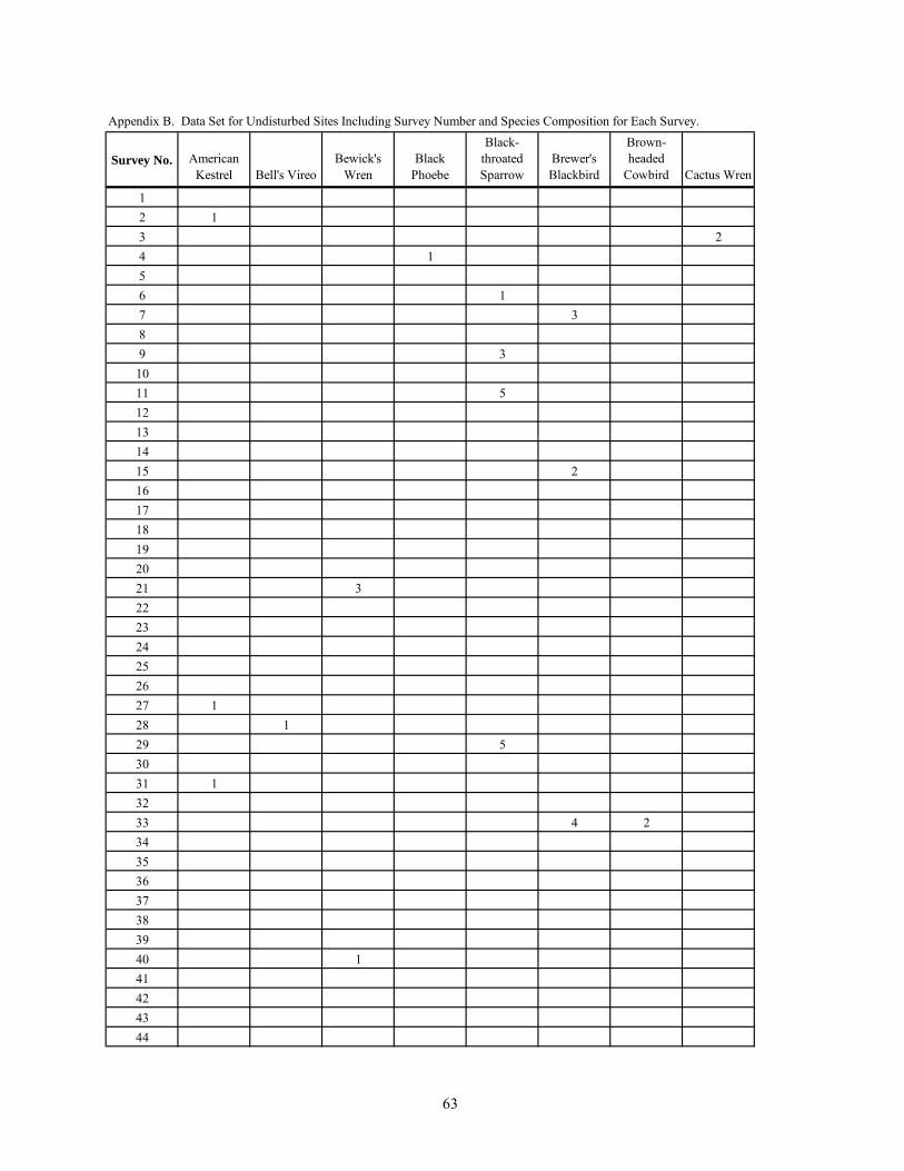
63
Appendix B. Data Set for Undisturbed Sites Including Survey Number and Species Composition for Each Survey.
Survey No. American Kestrel Bell's Vireo
Bewick's Wren
Black Phoebe
Black-throated Sparrow
Brewer's Blackbird
Brown-headed
Cowbird Cactus Wren
12 13 24 156 17 389 31011 512131415 2161718192021 3222324252627 128 129 53031 13233 4 234353637383940 141424344
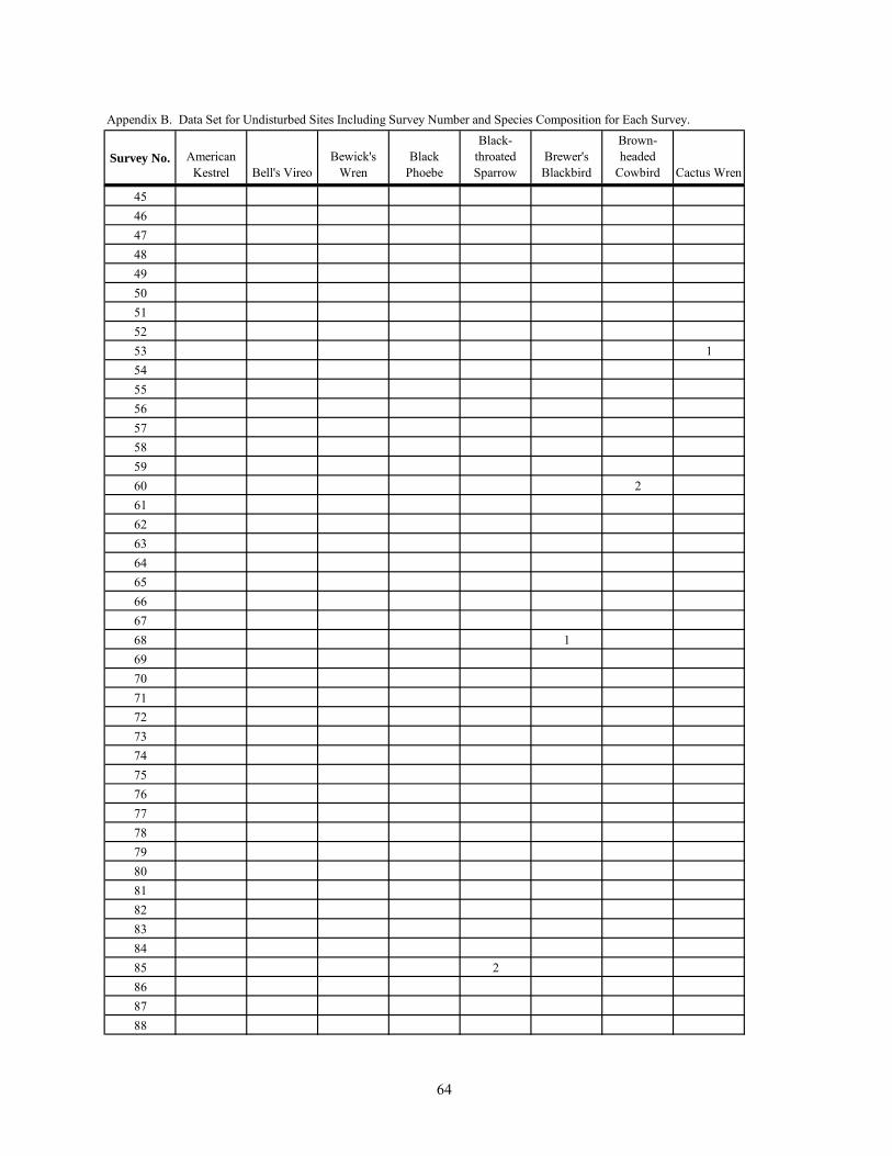
64
Appendix B. Data Set for Undisturbed Sites Including Survey Number and Species Composition for Each Survey.
Survey No. American Kestrel Bell's Vireo
Bewick's Wren
Black Phoebe
Black-throated Sparrow
Brewer's Blackbird
Brown-headed
Cowbird Cactus Wren
454647484950515253 154555657585960 26162636465666768 16970717273747576777879808182838485 2868788
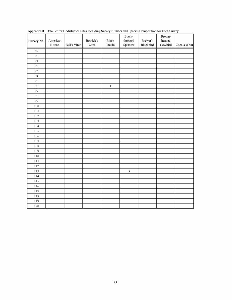
65
Appendix B. Data Set for Undisturbed Sites Including Survey Number and Species Composition for Each Survey.
Survey No. American Kestrel Bell's Vireo
Bewick's Wren
Black Phoebe
Black-throated Sparrow
Brewer's Blackbird
Brown-headed
Cowbird Cactus Wren
8990919293949596 1979899
100101102103104105106107108109110111112113 3114115116117118119120
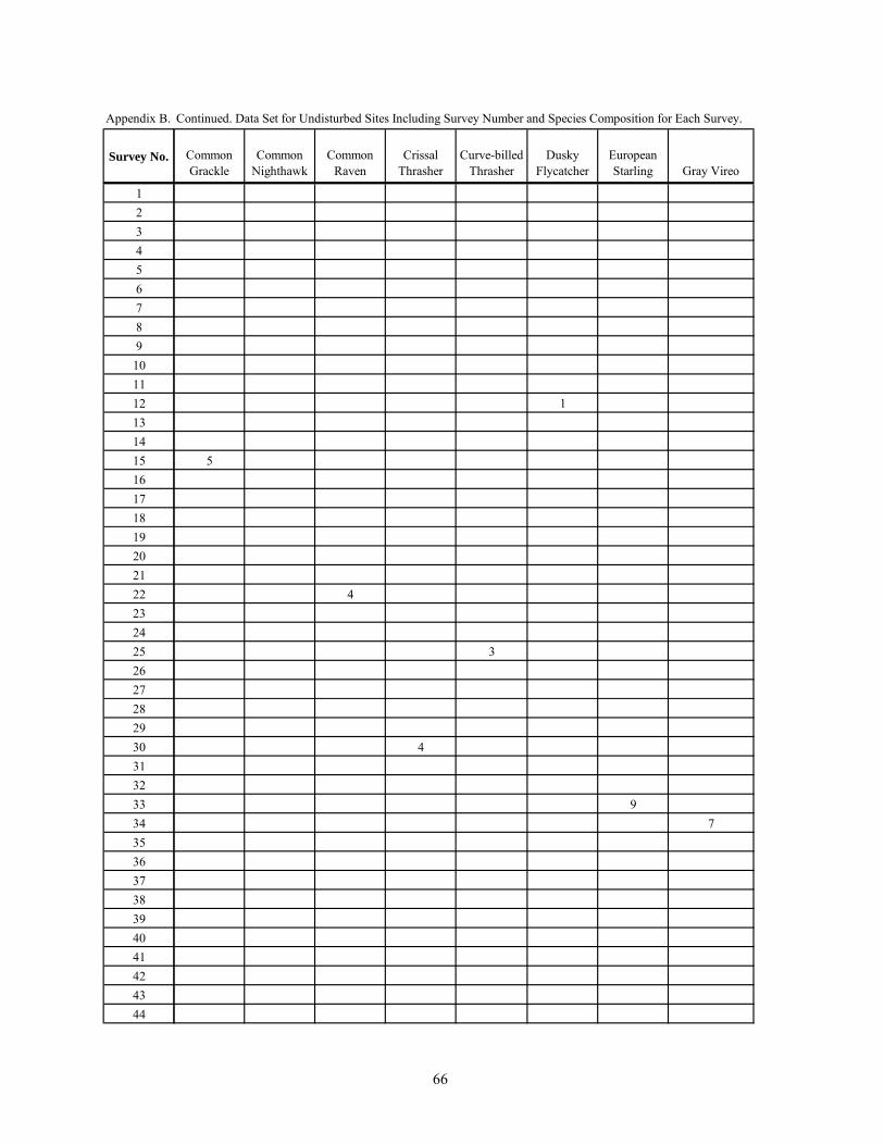
66
Appendix B.
Survey No.
1234567891011121314151617181920212223242526272829303132333435363738394041424344
Continued. Data Set for Undisturbed Sites Including Survey Number and Species Composition for Each Survey.
Common Grackle
Common Nighthawk
Common Raven
Crissal Thrasher
Curve-billed Thrasher
Dusky Flycatcher
European Starling Gray Vireo
1
5
4
3
4
97
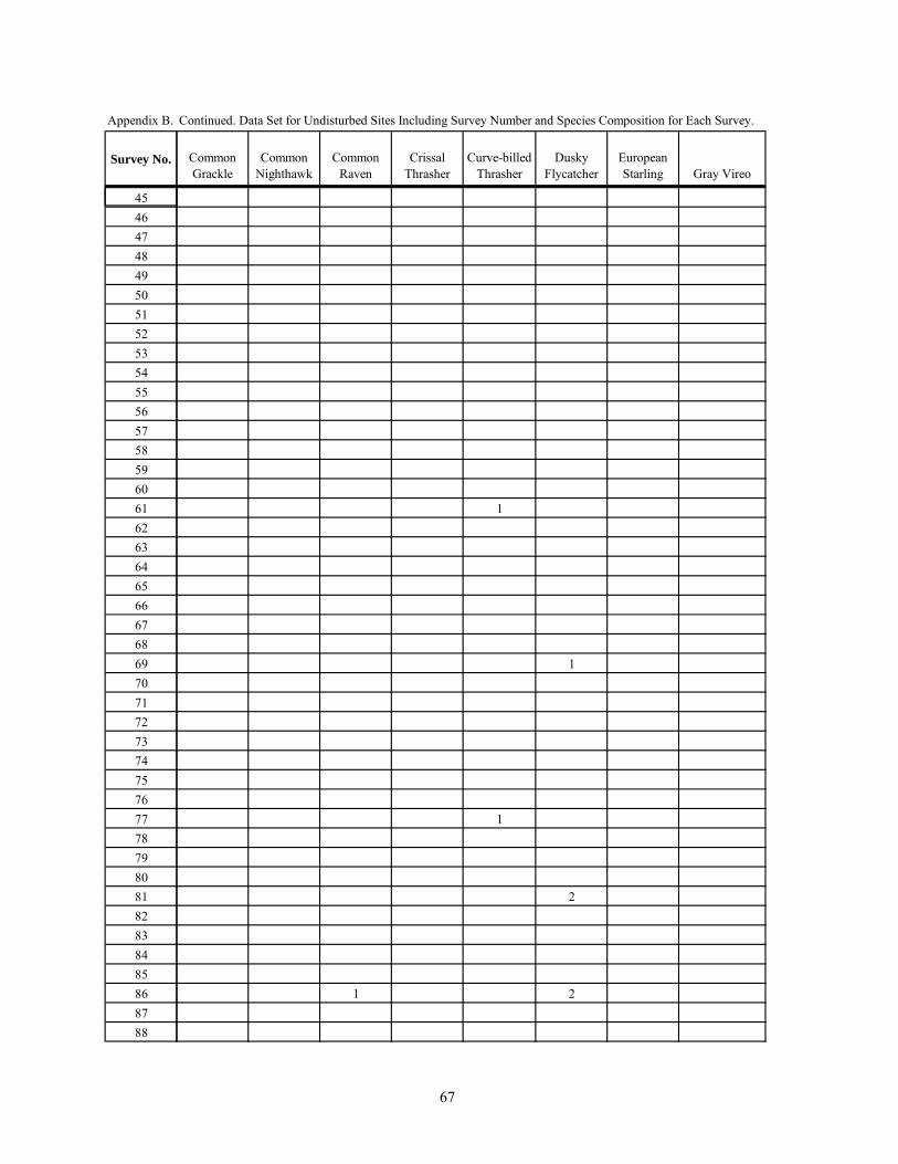
67
Appendix B.
Survey No.
4546474849505152535455565758596061626364656667686970717273747576777879808182838485868788
Continued. Data Set for Undisturbed Sites Including Survey Number and Species Composition for Each Survey.
Common Grackle
Common Nighthawk
Common Raven
Crissal Thrasher
Curve-billed Thrasher
Dusky Flycatcher
European Starling Gray Vireo
1
1
1
2
1 2
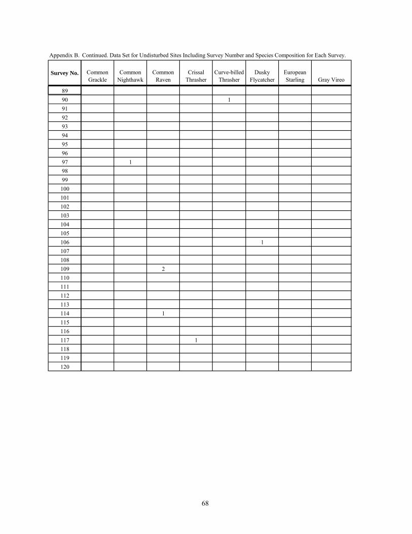
68
Appendix B.
Survey No.
8990919293949596979899
100101102103104105106107108109110111112113114115116117118119120
Continued. Data Set for Undisturbed Sites Including Survey Number and Species Composition for Each Survey.
Common Grackle
Common Nighthawk
Common Raven
Crissal Thrasher
Curve-billed Thrasher
Dusky Flycatcher
European Starling Gray Vireo
1
1
1
2
1
1
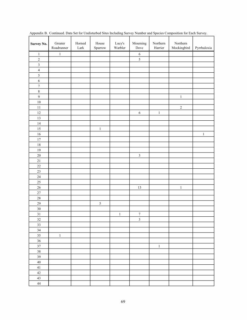
69
Appendix B.
Survey No.
1234567891011121314151617181920212223242526272829303132333435363738394041424344
Continued. Data Set for Undisturbed Sites Including Survey Number and Species Composition for Each Survey.
Greater Roadrunner
Horned Lark
House Sparrow
Lucy's Warbler
Mourning Dove
Northern Harrier
Northern Mockingbird Pyrrhuloxia
1 65
1
26 1
11
3
13 1
5
1 73
1
1
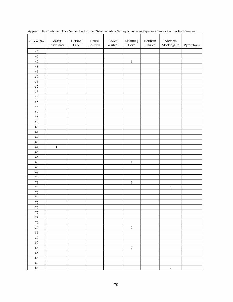
70
Appendix B.
Survey No.
4546474849505152535455565758596061626364656667686970717273747576777879808182838485868788
Continued. Data Set for Undisturbed Sites Including Survey Number and Species Composition for Each Survey.
Greater Roadrunner
Horned Lark
House Sparrow
Lucy's Warbler
Mourning Dove
Northern Harrier
Northern Mockingbird Pyrrhuloxia
1
1
1
11
2
2
2
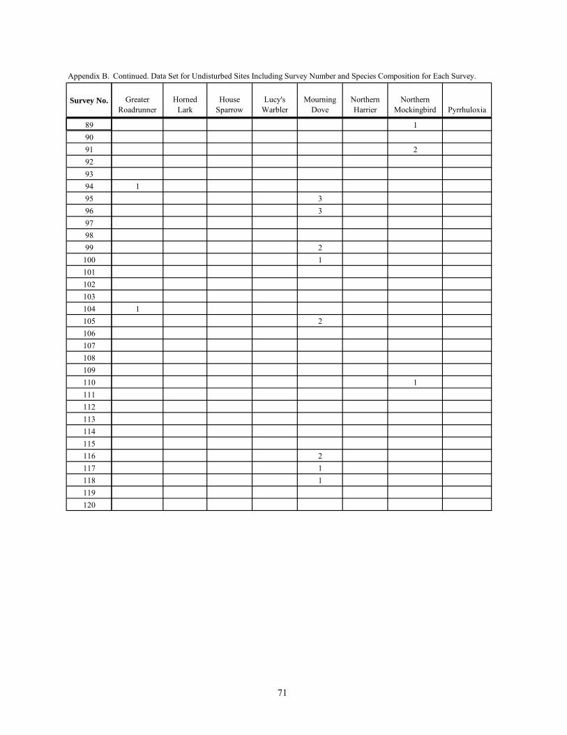
71
Appendix B.
Survey No.
8990919293949596979899
100101102103104105106107108109110111112113114115116117118119120
Continued. Data Set for Undisturbed Sites Including Survey Number and Species Composition for Each Survey.
Greater Roadrunner
Horned Lark
House Sparrow
Lucy's Warbler
Mourning Dove
Northern Harrier
Northern Mockingbird Pyrrhuloxia
1
2
133
21
12
1
211
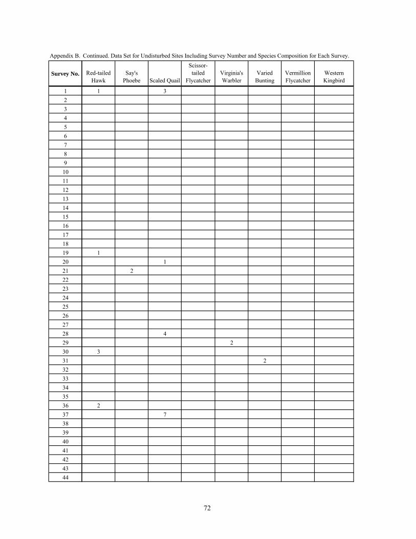
72
Appendix B.
Survey No.
1234567891011121314151617181920212223242526272829303132333435363738394041424344
Continued. Data Set for Undisturbed Sites Including Survey Number and Species Composition for Each Survey.
Red-tailed Hawk
Say's Phoebe Scaled Quail
Scissor-tailed
FlycatcherVirginia's Warbler
Varied Bunting
Vermillion Flycatcher
Western Kingbird
1 3
11
2
42
32
27
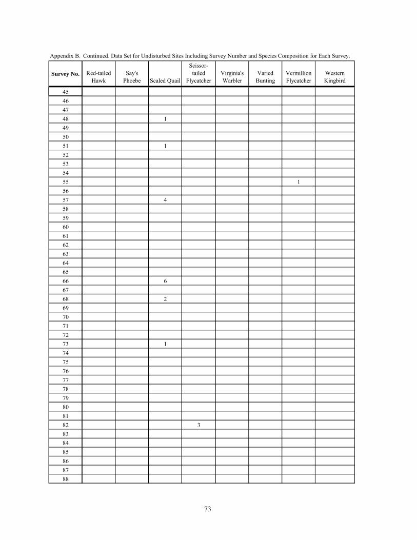
73
Appendix B.
Survey No.
4546474849505152535455565758596061626364656667686970717273747576777879808182838485868788
Continued. Data Set for Undisturbed Sites Including Survey Number and Species Composition for Each Survey.
Red-tailed Hawk
Say's Phoebe Scaled Quail
Scissor-tailed
FlycatcherVirginia's Warbler
Varied Bunting
Vermillion Flycatcher
Western Kingbird
1
1
1
4
6
2
1
3

74
Appendix B.
Survey No.
8990919293949596979899
100101102103104105106107108109110111112113114115116117118119120
Continued. Data Set for Undisturbed Sites Including Survey Number and Species Composition for Each Survey.
Red-tailed Hawk
Say's Phoebe Scaled Quail
Scissor-tailed
FlycatcherVirginia's Warbler
Varied Bunting
Vermillion Flycatcher
Western Kingbird
1
2
111
51
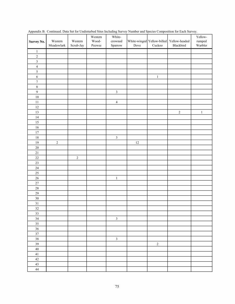
75
Appendix B.
Survey No.
1234567891011121314151617181920212223242526272829303132333435363738394041424344
Continued. Data Set for Undisturbed Sites Including Survey Number and Species Composition for Each Survey.
Western Meadowlark
Western Scrub-Jay
Western Wood-Peewee
White-crowned Sparrow
White-winged Dove
Yellow-billed Cuckoo
Yellow-headed Blackbird
Yellow-rumped Warbler
1
3
4
2 1
32 12
2
1
3
32
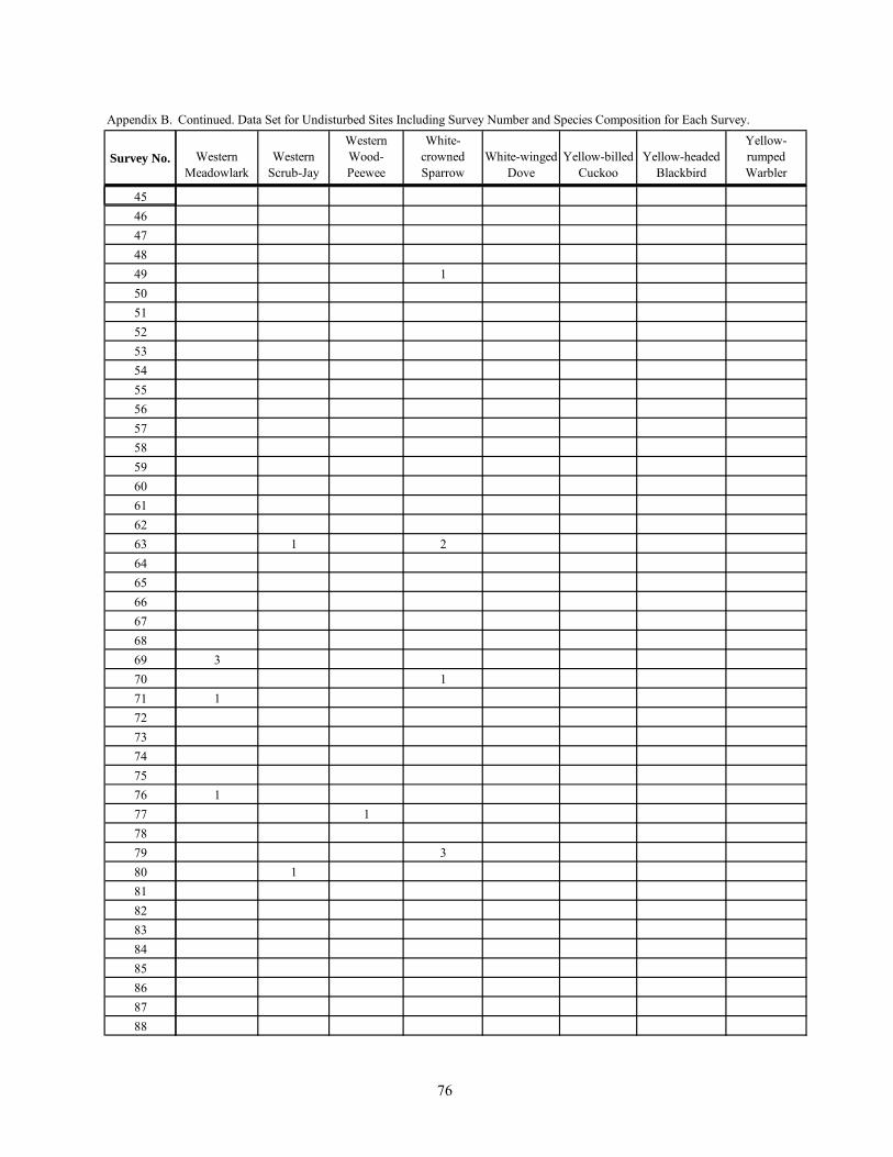
76
Appendix B.
Survey No.
4546474849505152535455565758596061626364656667686970717273747576777879808182838485868788
Continued. Data Set for Undisturbed Sites Including Survey Number and Species Composition for Each Survey.
Western Meadowlark
Western Scrub-Jay
Western Wood-Peewee
White-crowned Sparrow
White-winged Dove
Yellow-billed Cuckoo
Yellow-headed Blackbird
Yellow-rumped Warbler
1
1 2
31
1
11
31

77
Appendix B.
Survey No.
8990919293949596979899
100101102103104105106107108109110111112113114115116117118119120
Continued. Data Set for Undisturbed Sites Including Survey Number and Species Composition for Each Survey.
Western Meadowlark
Western Scrub-Jay
Western Wood-Peewee
White-crowned Sparrow
White-winged Dove
Yellow-billed Cuckoo
Yellow-headed Blackbird
Yellow-rumped Warbler
11
3
2
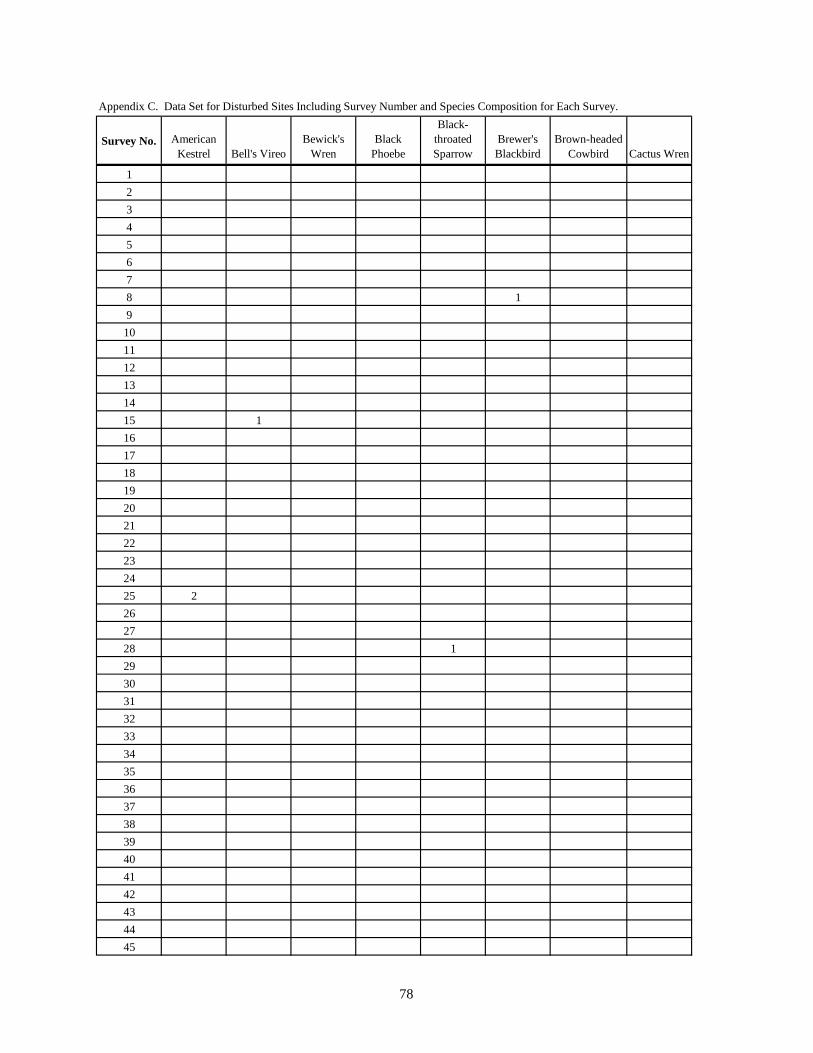
Appendix C. Data Set for Disturbed Sites Including Survey Number and Species Composition for Each Survey.
Survey No. American
Kestrel Bell's Vireo
Bewick's
Wren
Black
Phoebe
Black-
throated
Sparrow
Brewer's
Blackbird
Brown-headed
Cowbird Cactus Wren
1
2
3
4
5
6
7
8 1
9
10
11
12
13
14
15 1
16
17
18
19
20
21
22
23
24
25 2
26
27
28 1
29
30
31
32
33
34
35
36
37
38
39
40
41
42
43
44
45
78

Appendix C. Data Set for Disturbed Sites Including Survey Number and Species Composition for Each Survey.
Survey No. American
Kestrel Bell's Vireo
Bewick's
Wren
Black
Phoebe
Black-
throated
Sparrow
Brewer's
Blackbird
Brown-headed
Cowbird Cactus Wren
46
47
48
49
50
51 1
52
53
54
55
56
57
58
59
60
61
62
63
64
65
66
67
68
69
70
71
72
73
74
75
76
77
78
79
80
81
82
83
84
85
86
87
88
89
90
79

Appendix C. Data Set for Disturbed Sites Including Survey Number and Species Composition for Each Survey.
Survey No. American
Kestrel Bell's Vireo
Bewick's
Wren
Black
Phoebe
Black-
throated
Sparrow
Brewer's
Blackbird
Brown-headed
Cowbird Cactus Wren
91
92
93
94
95
96
97
98
99
100
101
102
103
104
105
106
107
108
109
110
111
112
113
114
115
116
80
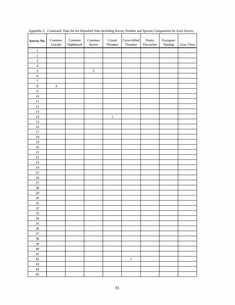
Appendix C. Data Set for Disturbed Sites Including Survey Number and Species Composition for Each Survey.
Survey No.
1
2
3
4
5
6
7
8
9
10
11
12
13
14
15
16
17
18
19
20
21
22
23
24
25
26
27
28
29
30
31
32
33
34
35
36
37
38
39
40
41
42
43
44
45
Continued. Data Set for Disturbed Sites Including Survey Number and Species Composition for Each Survey.
Common
Grackle
Common
Nighthawk
Common
Raven
Crissal
Thrasher
Curve-billed
Thrasher
Dusky
Flycatcher
European
Starling Gray Vireo
2
4
1
1
81

Appendix C. Data Set for Disturbed Sites Including Survey Number and Species Composition for Each Survey.
Survey No.
146
47
48
49
50
51
52
53
54
55
56
57
58
59
60
61
62
63
64
65
66
67
68
69
70
71
72
73
74
75
76
77
78
79
80
81
82
83
84
85
86
87
88
89
90
Continued. Data Set for Disturbed Sites Including Survey Number and Species Composition for Each Survey.
Common
Grackle
Common
Nighthawk
Common
Raven
Crissal
Thrasher
Curve-billed
Thrasher
Dusky
Flycatcher
European
Starling Gray Vireo
1
2
82

Appendix C. Data Set for Disturbed Sites Including Survey Number and Species Composition for Each Survey.
Survey No.
191
92
93
94
95
96
97
98
99
100
101
102
103
104
105
106
107
108
109
110
111
112
113
114
115
116
Continued. Data Set for Disturbed Sites Including Survey Number and Species Composition for Each Survey.
Common
Grackle
Common
Nighthawk
Common
Raven
Crissal
Thrasher
Curve-billed
Thrasher
Dusky
Flycatcher
European
Starling Gray Vireo
83
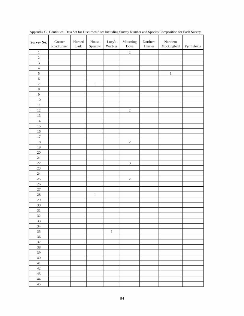
Appendix C. Data Set for Disturbed Sites Including Survey Number and Species Composition for Each Survey.
Survey No.
1
2
3
4
5
6
7
8
9
10
11
12
13
14
15
16
17
18
19
20
21
22
23
24
25
26
27
28
29
30
31
32
33
34
35
36
37
38
39
40
41
42
43
44
45
Continued. Data Set for Disturbed Sites Including Survey Number and Species Composition for Each Survey.
Greater
Roadrunner
Horned
Lark
House
Sparrow
Lucy's
Warbler
Mourning
Dove
Northern
Harrier
Northern
Mockingbird Pyrrhuloxia
2
1
1
2
2
3
2
1
1
84
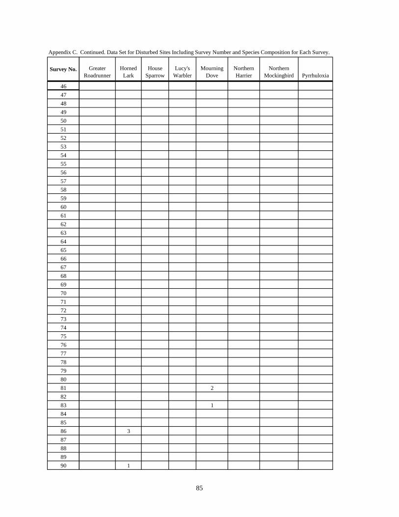
Appendix C. Data Set for Disturbed Sites Including Survey Number and Species Composition for Each Survey.
Survey No.
146
47
48
49
50
51
52
53
54
55
56
57
58
59
60
61
62
63
64
65
66
67
68
69
70
71
72
73
74
75
76
77
78
79
80
81
82
83
84
85
86
87
88
89
90
Continued. Data Set for Disturbed Sites Including Survey Number and Species Composition for Each Survey.
Greater
Roadrunner
Horned
Lark
House
Sparrow
Lucy's
Warbler
Mourning
Dove
Northern
Harrier
Northern
Mockingbird Pyrrhuloxia
2
1
3
1
85

Appendix C. Data Set for Disturbed Sites Including Survey Number and Species Composition for Each Survey.
Survey No.
191
92
93
94
95
96
97
98
99
100
101
102
103
104
105
106
107
108
109
110
111
112
113
114
115
116
Continued. Data Set for Disturbed Sites Including Survey Number and Species Composition for Each Survey.
Greater
Roadrunner
Horned
Lark
House
Sparrow
Lucy's
Warbler
Mourning
Dove
Northern
Harrier
Northern
Mockingbird Pyrrhuloxia
2
1
86

Appendix C. Data Set for Disturbed Sites Including Survey Number and Species Composition for Each Survey.
Survey No.
1
2
3
4
5
6
7
8
9
10
11
12
13
14
15
16
17
18
19
20
21
22
23
24
25
26
27
28
29
30
31
32
33
34
35
36
37
38
39
40
41
42
43
44
45
Continued. Data Set for Disturbed Sites Including Survey Number and Species Composition for Each Survey.
Red-tailed
Hawk
Say's
Phoebe Scaled Quail
Scissor-
tailed
Flycatcher
Virginia's
Warbler
Varied
Bunting
Vermillion
Flycatcher
Western
Kingbird
2
2
2
87

Appendix C. Data Set for Disturbed Sites Including Survey Number and Species Composition for Each Survey.
Survey No.
146
47
48
49
50
51
52
53
54
55
56
57
58
59
60
61
62
63
64
65
66
67
68
69
70
71
72
73
74
75
76
77
78
79
80
81
82
83
84
85
86
87
88
89
90
Continued. Data Set for Disturbed Sites Including Survey Number and Species Composition for Each Survey.
Red-tailed
Hawk
Say's
Phoebe Scaled Quail
Scissor-
tailed
Flycatcher
Virginia's
Warbler
Varied
Bunting
Vermillion
Flycatcher
Western
Kingbird
1
88

Appendix C. Data Set for Disturbed Sites Including Survey Number and Species Composition for Each Survey.
Survey No.
191
92
93
94
95
96
97
98
99
100
101
102
103
104
105
106
107
108
109
110
111
112
113
114
115
116
Continued. Data Set for Disturbed Sites Including Survey Number and Species Composition for Each Survey.
Red-tailed
Hawk
Say's
Phoebe Scaled Quail
Scissor-
tailed
Flycatcher
Virginia's
Warbler
Varied
Bunting
Vermillion
Flycatcher
Western
Kingbird
1
1
89
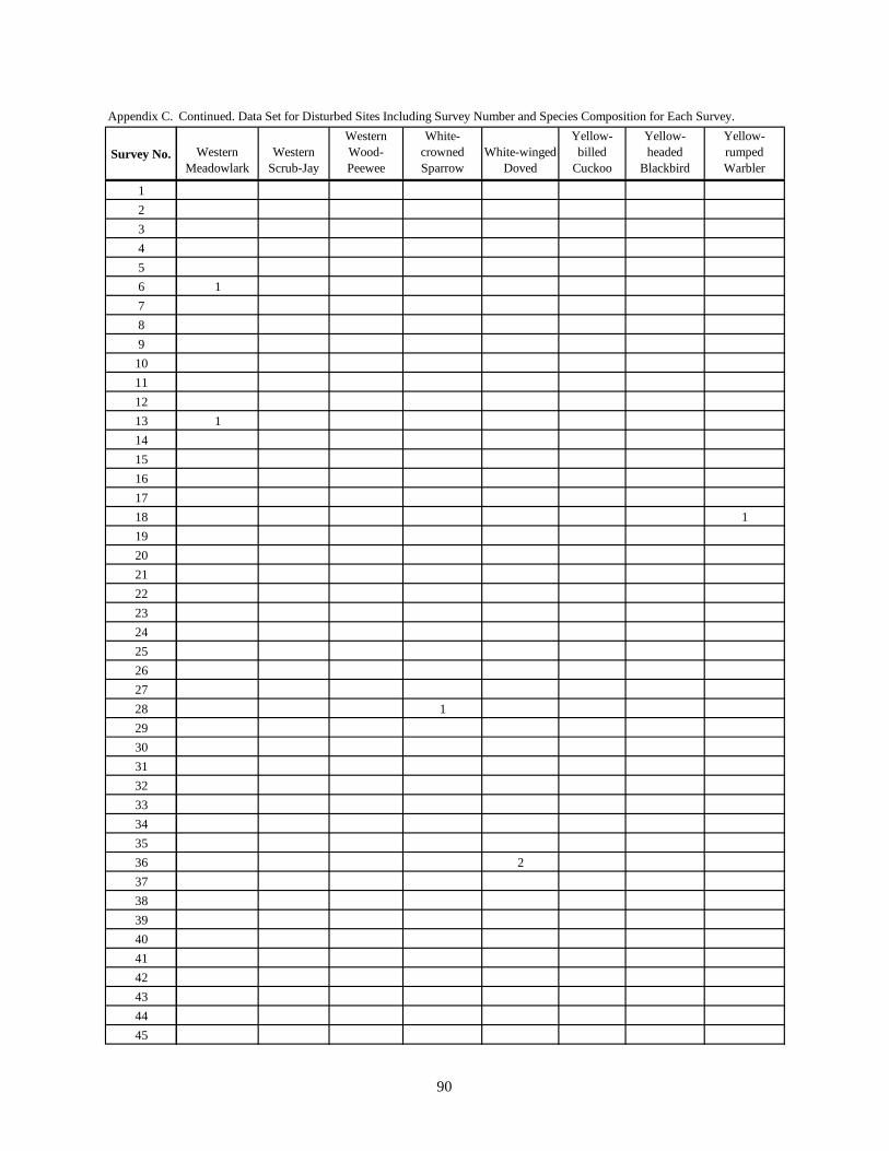
Appendix C. Data Set for Disturbed Sites Including Survey Number and Species Composition for Each Survey.
Survey No.
1
2
3
4
5
6
7
8
9
10
11
12
13
14
15
16
17
18
19
20
21
22
23
24
25
26
27
28
29
30
31
32
33
34
35
36
37
38
39
40
41
42
43
44
45
Continued. Data Set for Disturbed Sites Including Survey Number and Species Composition for Each Survey.
Western
Meadowlark
Western
Scrub-Jay
Western
Wood-
Peewee
White-
crowned
Sparrow
White-winged
Doved
Yellow-
billed
Cuckoo
Yellow-
headed
Blackbird
Yellow-
rumped
Warbler
1
1
1
1
2
90

Appendix C. Data Set for Disturbed Sites Including Survey Number and Species Composition for Each Survey.
Survey No.
146
47
48
49
50
51
52
53
54
55
56
57
58
59
60
61
62
63
64
65
66
67
68
69
70
71
72
73
74
75
76
77
78
79
80
81
82
83
84
85
86
87
88
89
90
Continued. Data Set for Disturbed Sites Including Survey Number and Species Composition for Each Survey.
Western
Meadowlark
Western
Scrub-Jay
Western
Wood-
Peewee
White-
crowned
Sparrow
White-winged
Doved
Yellow-
billed
Cuckoo
Yellow-
headed
Blackbird
Yellow-
rumped
Warbler
1
91

Appendix C. Data Set for Disturbed Sites Including Survey Number and Species Composition for Each Survey.
Survey No.
191
92
93
94
95
96
97
98
99
100
101
102
103
104
105
106
107
108
109
110
111
112
113
114
115
116
Continued. Data Set for Disturbed Sites Including Survey Number and Species Composition for Each Survey.
Western
Meadowlark
Western
Scrub-Jay
Western
Wood-
Peewee
White-
crowned
Sparrow
White-winged
Doved
Yellow-
billed
Cuckoo
Yellow-
headed
Blackbird
Yellow-
rumped
Warbler
92