hydrodynamic interaction in rotational...
TRANSCRIPT

HYDRODYNAMIC INTERACTION IN ROTATIONALFLOW
A Thesis Submitted tothe Graduate School of Engineering and Sciences of
Izmir Institute of Technologyin Partial Fulfillment of the Requirements for the Degree of
MASTER OF SCIENCE
in Mathematics
byFiliz CAGATAY
June 2007IZMIR

We approve the thesis of Filiz CAGATAY
Date of Signature
. . . . . . . . . . . . . . . . . . . . . . . . . . . . . . . . . . . . . 13 June 2007Prof. Dr. Oguz YILMAZSupervisorDepartment of MathematicsIzmir Institute of Technology
. . . . . . . . . . . . . . . . . . . . . . . . . . . . . . . . . . . . . 13 June 2007Prof. Dr. Oktay PASHAEVDepartment of MathematicsIzmir Institute of Technology
. . . . . . . . . . . . . . . . . . . . . . . . . . . . . . . . . . . . . 13 June 2007Prof. Dr. Gokmen TAYFURDepartment of Civil EngineeringIzmir Institute of Technology
. . . . . . . . . . . . . . . . . . . . . . . . . . . . . . . . . . . . . 13 June 2007
Prof. Dr. Oguz YILMAZHead of DepartmentDepartment of MathematicsIzmir Institute of Technology
. . . . . . . . . . . . . . . . . . . . . . . . . . . . . . . . . .Prof. Dr. M. Barıs OZERDEM
Head of the Graduate School

ACKNOWLEDGEMENTS
I would like to thank my advisor Prof.Dr Oguz Yılmaz for his continual advice,
supervision and understanding in research and writing of this thesis. I would also like
to thank Prof.Dr. Oktay Pashaev and Z. Nilhan Gurkan for their advices and supports
throughout my master studies. I would like to thank my family and Candas for their love
and infinite moral support.

ABSTRACT
HYDRODYNAMIC INTERACTION IN ROTATIONAL FLOW
The interaction of water waves with arrays of vertical cylinders problem is studied
using diffraction of water waves and addition theorem for bessel functions.
The linear boundary value problem which is derived from physical assumptions
is used as the approximate mathematical model for time-harmonic waves. Linearization
procedure is described for the nonlinear boundary conditions on the free surface. The
problem is solved by using Addition theorem for Bessel functions. Limiting case, k → 0,
known as long wave approximation, is analysed using limiting forms of Bessel functions.
Vortex-cylinder interaction is analyzed using a similar technique involving Lau-
rent series expansions of complex velocity and the Circle Theorem. But this method
failed to work. Further analysis is necessary. Vortex dynamics is analysed in annular do-
mains, which can conformally be mapped into infinite domain with two cylinders, using
the terminology of q-calculus.
Finally, the result of vortex-cylinder interaction in annular domain is transformed
into the infinite domain with two cylinders using conformal mapping. Image representa-
tion clearly shows the mechanism of inverse images which accumulate at zero and infinity
in the w-plane and a and 1/a in the z-plane.
iv

OZET
ROTASYONEL AKISTA HIDRODINAMIK ETKILESIM
Dikey yerlestirilmis silindirler arası su dalgası etkilesimi problemi, su dalgalarının
kırınımı ve Bessel fonksiyonlarının toplam teoremi (Addition theorem) kullanılarak
calısıldı.
Fiziksel kabullerden elde edilen, linear sınır deger problemi, zaman uyumlu dal-
galar icin yaklasık matematik modeli gibi kullanıldı. Serbest yuzeyde dogrusal olmayan
sınır sartları icin dogrusallastırma proseduru tanımlandı. Problem Bessel fonksiyonları
icin toplam teoremi kullanılarak cozuldu. Uzun dalga yaklasımı olarak da bilinen k → 0
limit durumu Bessel fonksiyonlarının limit formları kullanılarak incelenmistir.
Girdap (vortex)-silindir etkilesimi, karmasık hızın Laurent seri acılımı ve Cember
teoremi (Circle Theorem) iceren benzer yontem kullanılarak incelenebilir. Fakat henuz
gelistirilemedi. Halka bolgesindeki, konformal olarak iki silindirli sonsuz bolgeye
eslenebilen girdap dinamikleri, q- hesaplama terminolojisi kullanılarak incelenmistir.
Son olarak, halka bolgesindeki girdap-silindir etkilesim probleminin sonucu, uy-
gun donusum kullanılarak, iki silindirli sonsuz bolgeye donusturulur. Goruntu temsili,
ters goruntu isleyisinin(mekanızmasının), w-duzlemi icin sıfır ve sonsuzda, z-duzlemi
icinse a ve 1/a’da yıgıldıgını acıkca gosterir.
v

TABLE OF CONTENTS
LIST OF FIGURES . . . . . . . . . . . . . . . . . . . . . . . . . . . . . . . . x
CHAPTER 1 . INTRODUCTION . . . . . . . . . . . . . . . . . . . . . . . . . 1
CHAPTER 2 . BACKGROUND INFORMATION ABOUT HYDRODYNAMICS 2
2.1. Equations of Motion . . . . . . . . . . . . . . . . . . . . . . 2
2.1.1. Euler’s Equations . . . . . . . . . . . . . . . . . . . . . . 2
2.1.1.1. Incompressible Flows . . . . . . . . . . . . . . . . 4
2.1.1.2. Euler’s Equations for Incompressible Flows . . . . 4
2.1.1.3. Isentropic Fluids . . . . . . . . . . . . . . . . . . . 4
2.2. Rotation and Vorticity . . . . . . . . . . . . . . . . . . . . . 5
2.3. Potential Flow . . . . . . . . . . . . . . . . . . . . . . . . . 5
CHAPTER 3 . DIFFRACTION OF WATER WAVES BY MULTIPLE CYLINDERS 8
3.1. Nonlinear Problem . . . . . . . . . . . . . . . . . . . . . . . 8
3.1.1. Equations of Motion . . . . . . . . . . . . . . . . . . . . 8
3.1.2. Boundary Conditions . . . . . . . . . . . . . . . . . . . . 9
3.2. Linearization of the Problem . . . . . . . . . . . . . . . . . . 10
3.2.1. Equations for Small Amplitude Waves . . . . . . . . . . . 11
3.2.2. Boundary Condition on an Immersed Rigid Surface . . . . 12
3.3. Linearized Problem . . . . . . . . . . . . . . . . . . . . . . . 13
3.4. Linear Time-Harmonic Waves (The Water-Wave Problem) . . 13
3.5. Time Independent Problem . . . . . . . . . . . . . . . . . . . 14
3.5.1. Waves With No Bodies Present . . . . . . . . . . . . . . 14
3.5.2. Case of Single Cylinder . . . . . . . . . . . . . . . . . . 16
3.5.3. Multiple Cylinders in Progressive Waves . . . . . . . . . 17
3.5.4. Limiting Value of Velocity Potential as Wave Number
Approaches Zero(Long-Wave Approximation) . . . . . . 19
vi
CHAPTER 4 . VORTEX-CYLINDER INTERACTION IN FLOWS WITH
NO FREE SURFACE . . . . . . . . . . . . . . . . . . . . . . . 23
4.1. Complex Velocity . . . . . . . . . . . . . . . . . . . . . . . . 23
4.2. Complex Potential . . . . . . . . . . . . . . . . . . . . . . . 23
4.2.1. Complex Potential for a Vortex . . . . . . . . . . . . . . 24
4.2.2. Complex Velocity for a Vortex . . . . . . . . . . . . . . . 24
4.2.3. Streamlines of the Particle . . . . . . . . . . . . . . . . . 24
4.2.4. Boundary Conditions . . . . . . . . . . . . . . . . . . . . 24
4.3. Circle Theorem in Terms of Complex Velocity . . . . . . . . 25
4.4. The Circle Theorem for Complex Velocity . . . . . . . . . . . 26
4.4.1. Single Cylinder with a Vortex . . . . . . . . . . . . . . . 27
4.4.2. Multiple Cylinders with a Vortex . . . . . . . . . . . . . 27
4.4.3. Complex Velocity and Boundary Condition
for Cylinder j . . . . . . . . . . . . . . . . . . . . . . . . 27
CHAPTER 5 . VORTICES IN ANNULAR DOMAIN . . . . . . . . . . . . . . 29
5.1. Flow in Bounded Domain . . . . . . . . . . . . . . . . . . . 29
5.2. N Vortices in Annular Domain . . . . . . . . . . . . . . . . . 29
5.2.1. Algebraic System for Boundary Value Problem . . . . . . 30
5.2.2. Solution of Algebraic System . . . . . . . . . . . . . . . 31
5.2.3. Solution in Terms of q-logarithmic Function . . . . . . . 32
5.2.4. Complex Velocity and q-logarithm . . . . . . . . . . . . . 33
5.2.5. Vortex Image Representation . . . . . . . . . . . . . . . . 33
5.3. Complex Potential and Elliptic Functions . . . . . . . . . . . 35
5.4. Motion of a Point Vortex in Annular Domain . . . . . . . . . 36
CHAPTER 6 . CONFORMAL MAPPING OF ANNULAR DOMAIN ONTO
THE INFINITE DOMAIN WITH TWO CYLINDERS . . . . . . 38
6.1. Mobius Transformation and Mappings of the
Annular Domain . . . . . . . . . . . . . . . . . . . . . . . . 38
6.1.1. Equation of Circle . . . . . . . . . . . . . . . . . . . . . 38
6.1.2. Symmetry with Respect to Circle . . . . . . . . . . . . . 39
6.1.3. Mapping of Disc onto Unit Disc . . . . . . . . . . . . . . 41
vii

6.1.4. Mapping of Unit Disc onto Unit Disc . . . . . . . . . . . 42
6.1.5. Mapping of Two Cylinder onto Annular Domain . . . . . 44
6.2. Application of the Mobius Transformation to the
Vortex-Cylinder Problem . . . . . . . . . . . . . . . . . . . . 45
CHAPTER 7 . CONCLUSION . . . . . . . . . . . . . . . . . . . . . . . . . . 50
REFERENCES . . . . . . . . . . . . . . . . . . . . . . . . . . . . . . . . . . . 52
APPENDICES . . . . . . . . . . . . . . . . . . . . . . . . . . . . . . . . . . . 53
APPENDIX A. DIVERGENCE THEOREM . . . . . . . . . . . . . . . . . . . 53
A.1. Divergence Theorem . . . . . . . . . . . . . . . . . . . . . . 53
APPENDIX B. SEPARATION OF VARIABLES . . . . . . . . . . . . . . . . . 54
B.1. Solution of No Body Problem Using Separation of
Variables . . . . . . . . . . . . . . . . . . . . . . . . . . . . 54
APPENDIX C. BESSEL FUNCTIONS . . . . . . . . . . . . . . . . . . . . . . 56
C.1. Bessel’s Differential Equation . . . . . . . . . . . . . . . . . 56
C.2. Generating Function, Integral Order, Jn(x) . . . . . . . . . . 56
C.3. Integral Representation . . . . . . . . . . . . . . . . . . . . . 57
C.4. Standing Cylindrical Waves In terms of Bessel Functions . . . 57
C.5. Asymptotic Expansion for Large Arguments . . . . . . . . . . 58
C.5.1. Hankel’s Asymptotic Expansions . . . . . . . . . . . . . 58
C.6. Limiting Forms of Bessel Functions for Small Arguments . . 58
APPENDIX D. CAUCHY INTEGRAL FORMULA . . . . . . . . . . . . . . . 60
D.1. Cauchy Integral Formula . . . . . . . . . . . . . . . . . . . . 60
D.2. Complex Velocity Using Cauchy Integral Formula . . . . . . 60
D.2.1. No Singularity in C . . . . . . . . . . . . . . . . . . . . 60
D.2.2. One Singularity in C . . . . . . . . . . . . . . . . . . . . 61
D.2.3. N Singularity in C . . . . . . . . . . . . . . . . . . . . . 61
viii

D.2.4. Complex Velocity for One Cylinder . . . . . . . . . . . . 61
D.2.5. Complex Velocity for One Cylinder and One Vortex . . . 62
D.2.6. Complex Velocity for Two Cylinder and One Vortex . . . 64
D.2.7. Complex Velocity for K Cylinder and One Vortex . . . . 64
D.2.8. Complex Velocity for Two Cylinder and N Vortices . . . 64
D.3. Jacobi’s Expressions for the Theta-functions as
Infinite Products . . . . . . . . . . . . . . . . . . . . . . . . 64
ix

LIST OF FIGURES
Figure Page
Figure 3.1 Plan View of Two Cylinders. . . . . . . . . . . . . . . . . . . . . 17
Figure 3.2 Two Cylinder Case. . . . . . . . . . . . . . . . . . . . . . . . . . 20
Figure 4.1 Changing Coordinate System From ξi to ξj . . . . . . . . . . . . . 28
Figure 5.1 N Vortices in Annular Domain. . . . . . . . . . . . . . . . . . . . 30
Figure 5.2 Vortex Image Representation. . . . . . . . . . . . . . . . . . . . . 34
Figure 6.1 Mapping of D onto Unit Disc. . . . . . . . . . . . . . . . . . . . 41
Figure 6.2 Mapping of Unit Disc onto Unit Disc. . . . . . . . . . . . . . . . 42
Figure 6.3 Mapping of Given D onto Annular Domain. . . . . . . . . . . . . 42
Figure 6.4 Mapping of Two Cylinder onto Annular Domain . . . . . . . . . . 44
Figure 6.5 Inverses of w0 With Respect to circles |w| = R0 and |w| = 1. . . . 46
Figure 6.6 Inverses of 1/a With Respect to Circles |w| = R0 and |w| = 1. . . 46
Figure 6.7 Inverses of z0 With Respect to Circles |z| = 1 and |z − c| = ρ. . . 47
Figure 6.8 Vortex Image Approximation. . . . . . . . . . . . . . . . . . . . . 47
Figure 6.9 Images of w0 and 1/a. . . . . . . . . . . . . . . . . . . . . . . . . 48
Figure 6.10 Images of z0. . . . . . . . . . . . . . . . . . . . . . . . . . . . . . 49
x

CHAPTER 1
INTRODUCTION
The history of water wave theory is almost as old as that of partial differential
equations. Their founding fathers are the same: Euler, Lagrange, Cauchy, Poisson. Fur-
ther contributions were made by Stokes, Lord Kelvin, Kirchhoff, and Lamb who con-
structed a number of explicit solutions.
There are several expositions of the classical theory (Crapper(1984), Lamb(1932),
Lighthill(1978), Sretensky(1977), Stoker(1957), Wehausen & Laitone(1960) and
Whitham(1979)). Various aspects of the linear water waves have been considered in
works of Havelock and Ursell. Other works are focused on various applied aspects of the
theory. In particular, Haskind, Mei, Newman and Wehausen (Haskind(1973), Mei(1983),
Newman(1977, 1978) and Wehausen(1971))consider the wave-body interaction. Also,
there is the very recent monography by Linton and McIver (2001) on the mathematical
methods used in the theory of such interactions, but it mainly discusses mathematical
techniques from the point of view of their applications in ocean engineering.
The goal of present thesis is to study interaction in rotational flow. There are
several studies in interaction theory carried out by Linton & Evans, Spring & Monkmeyer
and Yilmaz(Linton & Evans (1990), Spring & Monkmeyer (1974) and Yilmaz (1994)).
Vortex dynamics was analysed by Pashaev & Gurkan and Gurkan & Pashaev (Pashaev &
Gurkan (2007) and Gurkan & Pashaev (2007)).
In Chapter 2 we solved the linear boundary value problem of diffraction of water
waves by arrays of vertical cylinders using Addition theorem for Bessel functions and
analysed long wave approximation using limiting forms of Bessel functions.
In Chapter 3 using Laurent series expansions of complex velocity and the Circle
Theorem we studied Vortex-cylinder interaction
In Chapter 4 we investigated vortex dynamics in annular domains using the termi-
nology of q-calculus.
Finally, Chapter 5, using the conformal mapping we transformed annular domain
onto infinite domain with two cylinders. We sketched the images of vortices.
1

CHAPTER 2
BACKGROUND INFORMATION ABOUT
HYDRODYNAMICS
2.1. Equations of Motion
2.1.1. Euler’s Equations
Let D be a region in two or three dimensional space filled with a fluid and bounded
by one or more moving or fixed surfaces that separate water from some other medium.
Our object is to describe the motion of such a fluid. Let x be a point in D and consider the
particle of fluid moving through x at time t. Relative to standard Euclidean coordinates in
space, we write x = (x, y, z). Imagine a particle (think of particle of dust suspended) in
the fluid; this particle traverses a well-defined trajectory. Let u(x, t) denote the velocity
of the particle of fluid that is moving through x at time t. Thus, for each fixed time, u
is a vector field on D. We call u the (spatial) velocity field of the fluid. For each time t,
assume that the fluid has a well-defined mass density ρ(x, t). Thus, if W is any subregion
of D, the mass of fluid in W at time t is given by
m(W, t) =
∫
W
ρ(x, t)dV, (2.1)
where dV is the volume element in the plane or in space. The assumption that ρ exists is
a continuum assumption. Clearly, it does not hold if the molecular structure of matter is
taken into account. For most macroscopic phenomena occurring in nature, it is believed
that this assumption is extremely accurate.
Our derivation of the equations is based on three basic principles:
i) Mass is neither created nor destroyed;
ii) The rate of change of momentum of a portion of the fluid equals the force ap-
plied to it(Newton’s Second Law.);
iii) Energy is neither created nor destroyed.
i) Conservation of Mass: The integral form of the conservation of mass is
d
dt
∫
W
ρdV = −∫
∂W
ρu.ndA, (2.2)
2

where ∂W is boundary of W . By the Divergence theorem (See Appendix A), equation
(2.2) is equivalent to ∫
W
[∂ρ
∂t+ div(ρu)]dV = 0. (2.3)
Because this holds for all W , (2.3) is equivalent to
∂ρ
∂t+ div(ρu) = 0. (2.4)
The equation (2.4) is the differential form of the law of conservation of mass, also known
as the continuity equation.
ii) Balance of Momentum: If W is region in the fluid at a particular instant of time t, the
total force exerted on the fluid inside W by means of stress on its boundary ∂W is
S∂W = (Force on W ) = −∫
∂W
pn dA (2.5)
where p is pressure. Divergence theorem gives
S∂W = −∫
W
grad p dV. (2.6)
If b(x, t) denotes the given body force per unit mass, the total body force is
B =
∫
W
ρb dV. (2.7)
Thus, on any piece of fluid material,
Force per unit volume = −grad p + ρb. (2.8)
By Newton’s Second Law (force=mass×acceleration) we are lead to the differential form
of the law of balance of momentum:
ρDu
Dt= −grad p + ρb, (2.9)
where DDt
= ∂∂t
+ u∇ is material derivative; it takes into account the fact that the fluid is
moving and that the position of fluid particles change with time.
iii) Conservation of Energy: For fluid moving in a domain D, with velocity field u, the
kinetic energy contained in a region W ⊂ D is
Ekinetik =1
2
∫
W
ρ||u||2dV. (2.10)
We assume that total energy of the fluid can be written as
Etotal = Ekinetik + Einternal (2.11)1
2
D
Dt||u||2 = u.
∂u
∂t+ u.(u.∇)u. (2.12)
3

2.1.1.1. Incompressible Flows
Definition 2.1 A flow is incompressible (Chorin and Marsden 1992) if for any fluid sub-
region W ,
divu = 0. (2.13)
2.1.1.2. Euler’s Equations for Incompressible Flows
Here we assume all the energy is kinetic and that the rate of change of kinetic energy in a
portion of fluid equals the rate at which the pressure and body forces do work;
d
dtEkinetic = −
∫
∂Wt
pu.ndA +
∫
Wt
ρu.b dV. (2.14)
Using the divergence theorem and since flow is incompressible, divu = 0 equation (2.14)
becomes, ∫
Wt
ρu.(∂u
∂t+ u.∇u)dV = −
∫
Wt
(u.∇p− ρu.b)dV. (2.15)
This argument, in addition, shows that if we assume E = Ekinetic, then the fluid must
be incompressible (unless p = 0). In summary, in this incompressible case, the Euler
equations are
ρDu
Dt= −grad p + ρb, (2.16)
Dρ
Dt= 0, (2.17)
divu = 0, (2.18)
with the boundary conditions
u.n = 0 on ∂D. (2.19)
2.1.1.3. Isentropic Fluids
A compressible flow will be called isentropic if there is a function ω, called the
enthalpy, such that
gradω =1
ρgradp. (2.20)
Given a fluid flow with velocity field u(x, t), a streamline at a fixed time is an
integral curve of u; that is, if x(s) is a streamline at the instant t, it is curve parametrized
by a variable, say s, that satisfies
dx
ds= u(x(s), t), t fixed.
4

We define a fixed trajectory to be the curve traced out by a particle as time progresses, as
explained at the beginning of this section. Thus a trajectory is a solution of the differential
equationdx
ds= u(x(t), t)
with suitable initial conditions. If u is independent of t streamlines and trajectory coin-
cide. In this case, the flow is called stationary.
Theorem 2.1 (Bernoulli’s Theorem) (Chorin and Marsden 1992) In stationary isen-
tropic flows and in the absence of external forces, the quantity
1
2||u||2 + ω (2.21)
is constant along streamlines. The same holds for homogeneous incompressible flow with
ω replaced by p/p0.
2.2. Rotation and Vorticity
The vector ∇× u = curlu ≡ ξ, called the vorticity vector. A vortex line is a line
drawn tangent to at each point in the direction of the vorticity vector. When the vorticity
vector is different from zero the motion is said to be rotational. A portion of the fluid
at every point of which the vorticity is zero is said to be irrotational motion. In such a
portion of the fluid there are no vortex lines.
Let C be a simple closed contour in the fluid at t = 0. Let Ct be the contour
carried along by the flow at time t. In other words,
Ct = ϕt(C), (2.22)
where ϕt is the fluid flow map. The circulation around Ct is defined to be the line integral
ΓCt =
∮
Ct
u.ds. (2.23)
Theorem 2.2 (Kelvin’s Circulation Theorem) (Chorin and Marsden 1992) For isen-
tropic flow without external forces, the circulation, ΓCt is constant in time.
2.3. Potential Flow
An inviscid, irrotational flow is called a potential flow. A domain D is called
simply connected if any continuous closed curve in D can be continuously shrunk to a
5

point without leaving D. For example, in space, the exterior of a solid sphere is simply
connected, whereas in the plane the exterior of a solid disc is not simply connected. For
irrotational flow in a simply connected region D, there is a scalar function φ(x, t) on D
called velocity potential such that for each t, u = gradφ. It follows that the circulation
around any closed curve C in D is zero. In particular, if the flow is stationary,
1
2‖ u ‖2 + w = constant in space. (2.24)
For the last equation to hold, simple connectivity of D is unnecessary. For potential flow
in nonsimply connected domains, it can occur that the circulation ΓC around closed curve
C is nonzero. For instance, consider
u = (−y
x2 + y2,
x
x2 + y2) (2.25)
outside the origin. If the contour C can be deformed within D to another contour C ′, then
ΓC = ΓC′ . The reason is that basically C ∪ C′ forms the boundary of a surface
∑in D.
Stokes’ theorem then gives∫P ξ.dA =
∫
C
u.ds−∫
C′u.ds = ΓC − ΓC′ (2.26)
and because ξ = 0 in D, we get ΓC = ΓC′ . From Kelvin’s Circulation theorem, the
circulation around a curve is constant in time. Thus, the circulation around an obstacle
in the plane is well-defined and constant in time. Next, consider incompressible potential
flow in a simply connected domain D. From u = gradφ and div u = 0, we have
∆φ = 0. (2.27)
Let the velocity of ∂D be specified as V, so
un = Vn. (2.28)
Thus, φ solves the Neumann Problem:
∆φ = 0,∂φ
∂n= V.n. (2.29)
If φ is a solution of the equation (2.29), then u = gradφ is a solution of the stationary
homogeneous Euler equations, i.e.,
ρ(u.∇)u = −gradp, (2.30)
div u = 0, (2.31)
u.n = V.n on ∂D, (2.32)
6
where p = ρ‖ u ‖2/2.
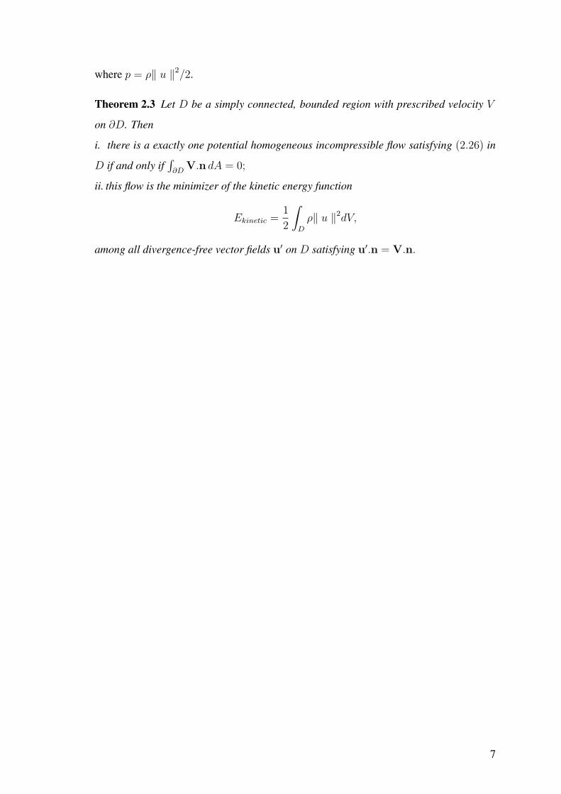
Theorem 2.3 Let D be a simply connected, bounded region with prescribed velocity V
on ∂D. Then
i. there is a exactly one potential homogeneous incompressible flow satisfying (2.26) in
D if and only if∫
∂DV.n dA = 0;
ii. this flow is the minimizer of the kinetic energy function
Ekinetic =1
2
∫
D
ρ‖ u ‖2dV,
among all divergence-free vector fields u′ on D satisfying u′.n = V.n.
7

CHAPTER 3
DIFFRACTION OF WATER WAVES BY MULTIPLE
CYLINDERS
3.1. Nonlinear Problem
3.1.1. Equations of Motion
The conservation of mass implies the continuity equation
∂ρ
∂t+ div(ρu) = 0 in W. (3.1)
Under the assumption that the fluid is incompressible (which is usual in the water wave
theory), equation (3.1) becomes
divu = 0 in W. (3.2)
The conservation of momentum in inviscid fluid leads to the so called Euler Equations.
Taking into account the gravity force, one can write last two equations in the following
vector form:
ut + u.∇u = −ρ−1∇p + g. (3.3)
Here g is the vector of the gravity force having zero horizontal components and the ver-
tical one equal to −g where g denotes the acceleration caused by gravity. An Irrotational
character of motion is another usual assumption in the water-wave theory; that is
rotu = 0 in W. (3.4)
Equation (3.4) guarantees the existence of a velocity potential φ, so that
u = ∇φ in W. (3.5)
From (3.2) and (3.5) one obtains the Laplace equation
∆φ = 0 in W. (3.6)
This greatly facilitates the theory but, in general solutions of (3.6) do not manifest wave
character. Waves are created by the boundary conditions on the free surface.
8

3.1.2. Boundary Conditions
We consider boundaries of two types: free surface separating water from the at-
mosphere and rigid surfaces of bodies floating in and/or beneath the free surface.
Let y = η(x, t) be the equation of the free surface. The pressure is prescribed to
be equal to the constant atmospheric pressure p0 on y = η(x, t). From (3.3) and (3.5) we
can obtain Bernoulli’s equation,
∂φ
∂t+|∇φ|2
2= −p
ρ− gy + c(t) in W . (3.7)
On the free surface y = η(x, t), p = p0 and c(t) = p0
ρ. We get the dynamic boundary
condition on the free surface:
∂φ
∂t+|∇φ|2
2+ gη(x, t) = 0 for y = η(x, t), x ∈ F. (3.8)
Another boundary condition holds on every ”physical” surface S bounding the
fluid domain W. Let S(x, y, t) = 0 be equation of S, then
DS
Dt= 0 on S (3.9)
DS
Dt=
∂S
∂t+ u∇S = 0 on S (3.10)
∂S
∂t= −u∇S, ∇S = |∇S|n (3.11)
−∂S
∂t= u |∇S|n (3.12)
un =1
|∇S|∂S
∂t= υn (3.13)
where υn denotes the normal velocity of S. Thus the kinematic boundary condition means
that the normal velocity of particles is continuous across a physical boundary. On the other
hand,
∇S =∂S
∂xi +
∂S
∂yj (3.14)
0 =∂S
∂xdx +
∂S
∂ydy +
∂S
∂tdt (3.15)
∂S
∂t= −∂S
∂x
dx
dt− ∂S
∂y
dy
dt(3.16)
∂S
∂t= −∇S υ (3.17)
un = − 1
| ∇S | (∇S υ) (3.18)
υn = un. (3.19)
9

We obtained the kinematic boundary condition on S,
un = υ n on S. (3.20)
On the fixed part of S, (3.20) takes the form of,
∂φ
∂n= 0 on S. (3.21)
On the free surface, condition (3.10), written as follows,
ηt + φx.ηx − φy = 0 y = η(x, t), x ∈ F, (3.22)
complements the dynamic condition (3.8). Thus, in the present approach, two nonlinear
conditions (3.8) and (3.22) on the unknown boundary are responsible for waves, which
constitute the main characteristic feature of water-surface wave theory.
In the water-wave problem one seeks the velocity potential φ(x, y, t) and the free
surface elevation η(x, t) satisfying
∇2φ = 0 in W, (3.23)∂φ
∂t+| ∇φ |2
2+ gη(x, t) = 0 for y = η(x, t), x ∈ F, (3.24)
ηt + φx, ηx − φy = 0 y = η(x, t), x ∈ F, (3.25)∂φ
∂n= un on W . (3.26)
The initial values of φ and η should also be prescribed, as well as the conditions at in-
finity (for unbounded W ) to complete the problem, which is known as Cauchy-Poisson
Problem.
3.2. Linearization of the Problem
There is a mathematical evidence that the linearized problem provides an approx-
imation to the nonlinear one. More precisely, under the assumption that the undisturbed
water occupies a layer of constant depth, the followings are proved:
1. The nonlinear problem is solvable for sufficiently small values of the linearization
parameter.
2. As this parameter tends to zero, solutions of the nonlinear problem do converge to
the solution of the linearized problem in the norm of some suitable function space.
10
To be in a position to describe water waves in the presence of bodies, the equations should
be approximated by more tractable ones. The usual and rather reasonable simplification
consist of a linearization of the problem under certain assumptions concerning the motion
of a floating body. An example of such assumptions (there are other ones leading to the
same conclusions) suggest that a body’s motion near the equilibrium position is so small
that it produces only waves having a small amplitude and small wavelength. There are
three characteristic geometry parameters:
1. A typical value of the wave height H .
2. A typical wavelength L.
3. The water depth D.
They give the three characteristic quotients : H/L, H/D, and L/D. The relative impor-
tance of these quotients is different in different situations. If
H
D¿ 1 and
H
L
(L
D
)3
¿ 1, (3.27)
then the linearization can be justified by some heuristic considerations. The last parameter
(H/L)(L/D)3 = (H/D)(H/D)2 is usually referred to as Ursell’s number.
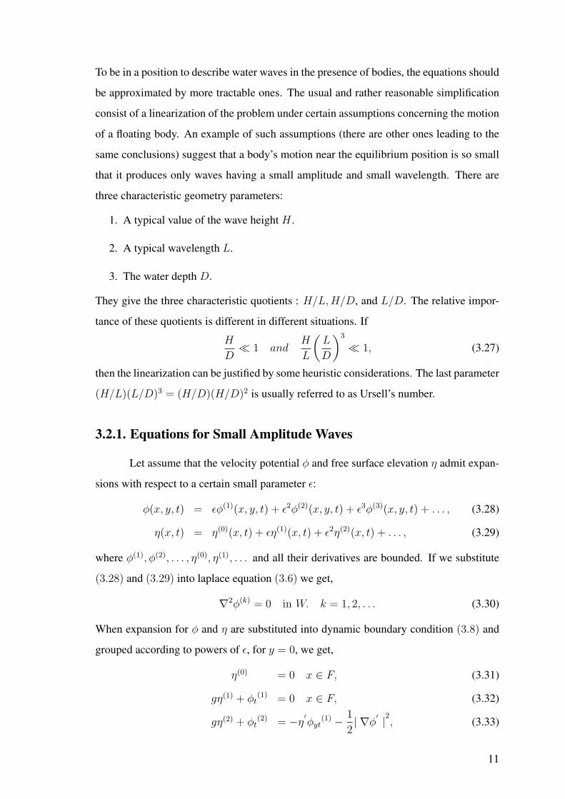
3.2.1. Equations for Small Amplitude Waves
Let assume that the velocity potential φ and free surface elevation η admit expan-
sions with respect to a certain small parameter ε:
φ(x, y, t) = εφ(1)(x, y, t) + ε2φ(2)(x, y, t) + ε3φ(3)(x, y, t) + . . . , (3.28)
η(x, t) = η(0)(x, t) + εη(1)(x, t) + ε2η(2)(x, t) + . . . , (3.29)
where φ(1), φ(2), . . . , η(0), η(1), . . . and all their derivatives are bounded. If we substitute
(3.28) and (3.29) into laplace equation (3.6) we get,
∇2φ(k) = 0 in W. k = 1, 2, . . . (3.30)
When expansion for φ and η are substituted into dynamic boundary condition (3.8) and
grouped according to powers of ε, for y = 0, we get,
η(0) = 0 x ∈ F, (3.31)
gη(1) + φt(1) = 0 x ∈ F, (3.32)
gη(2) + φt(2) = −η
′φyt
(1) − 1
2| ∇φ
′ |2, (3.33)
11

and so on; that is all these conditions hold on the mean position of the free surface at rest.
Similarly, the kinematic condition (3.22) leads to
(εηt(1) + ε2ηt
(2)) + (εηx(1) + ε2ηx
(2)).(εφx(1) + ε2φyx
(1)η(1) + ε2φx(2))
− (εφy(1) + ε2φyy
(1)η(1) + ε2φy(2)) = 0. (3.34)
After grouping, we obtain,
φy(1) − ηt
(1) = 0 x ∈ F, (3.35)
φy(2) − ηt
(2) = φx(1)ηx
(1) − φyy(1)η(1). (3.36)
By eliminating η(1) between (3.32) and (3.35), one finds the classical first order linear
free surface condition,
g φy(1) + φtt
(1) = 0 for y = 0 , x ∈ F. (3.37)
In the same way, one obtains from (3.33) and (3.36) the following,
g φy(2)+φtt
(2) = −φt(1)(φ(1)
x )2− 1
g2[φt
(1)φttt(1)+| ∇xφ
(1) |2] for y = 0, x ∈ F. (3.38)
All these conditions have the same operator on the left-hand side and the right-hand term
depends nonlinearly on terms of smaller orders.
3.2.2. Boundary Condition on an Immersed Rigid Surface
The homogeneous Neumann condition (3.21) is linear on fixed surfaces. The sit-
uation reverses for the nonhomogeneous Neumann condition (3.13) on a moving surface
S. It is convenient to carry out linearization locally. If linearization is done as we did
before, we get linearized boundary condition:
∂φ(1)/∂n = v(1)n on S, (3.39)
where
v(1)n = ζ
(1)t /[1+ | ∇ξζ
(0) |2]1/2,
is the first-order approximation of the normal velocity of S(t, ε).
12

3.3. Linearized Problem
As a result we can write boundary value problem for the first-order velocity poten-
tial φ(1)(x, y, t). It is defined in W occupied by water at rest with a boundary consisting
of the free surface F , the bottom B, and the wetted surface of immersed bodies S and it
must satisfy
∇2φ(1) = 0 in W, (3.40)
φtt(1) + gφy
(1) = 0 x ∈ F, (3.41)
∂φ(1)/∂n = v(1)n on S, (3.42)
∂φ(1)/∂n = 0 on B, (3.43)
φ(1)(x, 0, 0) = φ0(x), (3.44)
φ(1)t (x, 0, 0) = −gη0(x), (3.45)
where φ0, v(1)n and η0 are given functions and η0(x) = η(1)(x, 0).
3.4. Linear Time-Harmonic Waves (The Water-Wave Problem)
Since our study is concerned with the steady-state problem of scattering of water
waves by bodies floating in/or beneath the free surface, we assume all motions to be
simple harmonic in time. The corresponding frequency is denoted by ω. Thus, the right-
hand-side (3.39) is
v(1)n = Ree−iωtf on S, (3.46)
where f is complex function independent of t and fist-order velocity potential φ(1) can be
written in the form,
φ(1)(x, y, t) = Ree−iωtφ(x, y). (3.47)
A complex function φ in (3.47) is also referred to as velocity potential (this does not lead
to confusion, because it will always be clear what kind of time dependence is considered).
u is defined in the fixed domain W occupied by water at rest outside any bodies present.
The boundary ∂W consists of three disjoint sets:
i. S, is the union of the wetted surfaces of bodies in equilibrium;
ii. F , denotes the free surface at rest that is the part of y = 0 outside all the bodies;
13

iii. B, denotes the bottom positioned below F ∪ S.
Sometimes we will consider W unbounded below and corresponding to infinitely deep
water. In this case ∂W = F ∪ S.
3.5. Time Independent Problem
Substituting (3.46) and (3.47) into (3.40)− (3.45) gives the boundary value prob-
lem for φ
∇2φ = 0 in W, (3.48)
gφy − ω2φ = 0 on F, (3.49)
∂φ/∂n = f on S, (3.50)
∂φ/∂n = 0 on B. (3.51)
Normal n to a surface always directed into the water domain W . For deep water (B = ∅),
condition (∂φ/∂n = 0) should be replaced by the following one,
|∇φ| → 0 as y → −∞ (3.52)
that is, the water motion decays with depth. A natural requirement that a solution to
(3.48) − (3.52) should be unique also imposes a certain restriction on the behavior of φ
as |x| → ∞. This is known as Radiation Condition.
3.5.1. Waves With No Bodies Present
Example 3.1 (Waves With No Bodies Present) As an example we can consider waves
existing in the absence of bodies. For a layer W of constant depth d,
F = x ∈ R2, y = 0
is the free surface and
B = x ∈ R2, y = −d
is the bottom.
14

Solution : We can write the problem,
∇2φ = 0 in W,
φy − νφ = 0 on F, (3.53)
∂φ
∂y= 0 on B.
The corresponding potential can be easily obtained by separation of variables (see Ap-
pendix B)
φ =cosh k(y + d)
cosh(kd)(c1eikx + c2e−ikx) (3.54)
φ1 = <
cosh k(y + d)
cosh(kd)(c1eikx−iωt + c2e−ikx−iωt)
(3.55)
in which c1, c2 any constants and k = |k| =√
k21 + k2
2. If c2 = 0, we get plane pro-
gressive wave. A plane progressive wave propagating in the direction of a wave vector
k = (k1, k2) has the velocity potential
φ =cosh k(y + d)
cosh kd
(c1eikx
), (3.56)
φ(1) = <cosh k(y + d)
cosh kd(c1eikx−iωt)
. (3.57)
If the coefficients in equation (3.54) are identical, progressive waves propagating in op-
posite directions give a standing wave. Standing cylindrical wave in water layer of depth
d has the following potential (see Appendix C),
φ(1) = <Aeikx−iωtcosh k(y + d) + <Ae−ikx−iωtcosh k(y + d) (3.58)
= <
2Ae−iωt
∞∑n=−∞
cos[n(π
2− θ)]Jn(kr)
cosh[k(y + d)]. (3.59)
Here r = |x|, A = c1/cosh kd and J0 denotes the Bessel function of order zero (see Ap-
pendix C). Then a standing cylindrical wave in a water layer of depth d has the following
potential,
C1 cos(ωt)J0(kr) cosh[k(y + d)], (3.60)
where C1 is a real constant.
When J0 replaced by H0, which is another solution of Bessel’s equation, we can
obtain a cylindrical wave having arbitrary phase at infinity. This allows one to construct a
potential of outgoing waves as follows,
<C2 cos(ωt)H0
(1)(kr) cosh[k(y + d)]e−iωt. (3.61)
15

C2 is a complex constant and H0(1) denotes the first Hankel function of order zero. Out-
going behavior of this wave becomes clear from the asymptotic formula (see Appendix
C).
3.5.2. Case of Single Cylinder
Example 3.2 (Case of Single Cylinder)
Solution : Since there is a cylinder with radius a and with fixed position, only difference
from previous example is boundary condition on S. Then we can write
∇2φ = 0 in W,
φy − νφ = 0 on F,
∂eφ∂y
= 0 on B, (3.62)
∂eφ∂n
= 0 on S.
For the problem we can decompose φ as a combination of incident and diffracted waves,
φ = φd + φi .
WithoutBodies WithBodies
∇2φi = 0 in W ∇2φd = 0 in W
φiy − νφi = 0 on F φdy − νφd = 0 on F
∂eφi
∂y= 0 on B ∂eφd
∂y= 0 on B
∂eφi
∂n= −∂eφd
∂non S.
For the case without body, there are only incident waves
φi = Re
Ae−iωt
∞∑n=−∞
Jn(kr)ein(π2−θ)
cosh[k(y + d)]. (3.63)
For the diffracted waves we can construct a potential of outgoing waves
φd = Re
Ae−iωt
∞∑n=−∞
CnHn(1)(kr)ein(π
2−θ)
cosh[k(y + d)]. (3.64)
If we apply boundary condition ∂eφi
∂n= −∂eφd
∂non r = a, a is the radius of cylinder, we can
find the unknown coefficient
Cn = −Jn′(ka)
H ′n(ka)
. (3.65)
16

3.5.3. Multiple Cylinders in Progressive Waves
Now we assume that there are N(> 1) fixed vertical cylinders each of which
extends from the bottom, z = −d up to the free surface. We will use N + 1 coordinate
systems: (r, θ) are polar coordinates in the (x1, x2)-plane. (rj, θj), are polar coordinates
and (x1j, x2j) are cartesian coordinates, (j = 1, . . . , N), centered at (x01j, x
02j) which is
the center of the jth cylinder. (see Figure 3.1)
6
-
6
-
6
-
x1
x2
x1j
x2j
x1i
x2i
¢¢¢
½¼
¾»½¼
¾»
³³³³³³³³³³³³
¢¢¢¢¢¢¢¢¢
Rij
rirj
β
θj
θi
x01j
x02j
Figure 3.1. Plan View of Two Cylinders.
An incident plane wave making an angle β with the x-axis is characterized by
φI = eik(x1 cos β+x2 sin β). (3.66)
If we put x1 = r cos θ and x2 = r sin θ,
φI = eikr cos(θ−β), (3.67)
Since
x1 = x01j + x1j, x1j = rj cos θj (3.68)
x2 = x02j + x2j, x2j = rj sin θj (3.69)
17

φI for jth cylinder
φjI = eik(x1 cos β+x2 sin β) (3.70)
= eik((x01j+x1j) cos β+(x0
2j+x2j) sin β) (3.71)
= eik((x01j+rj cos θj) cos β+(x0
2j+rj sin θj)sinβ) (3.72)
= Ijeikrj cos(θj−β) (3.73)
where Ij(= eik(x01j cos β+x0
2j sin β)) is a phase factor associated with cylinder j.
Incident wave with respect to cylinder j can be written,
φjI = Ij
∞∑n=−∞
Jn(krj)ein(π/2+β−θj) = Ij
∞∑n=−∞
Jn(krj)ein(π/2−β)einθj . (3.74)
A general form for diffracted wave emanating from cylinder i,
φid = Ii
∞∑n=−∞
AinHn(kri)e
in(π/2−θi+β). (3.75)
Using Graf’s addition theorem for Bessel functions (see Appendix C) we can express
(3.75) in terms of the coordinates (rj, θj)
φid = Ii
∞∑n=−∞
Aine
in(π/2−β)
∞∑
l=−∞Hn−l(kRij)e
iαij(n−l)Jl(krj)eilθj ,
where Rij is the distance between the center of cylinder j and cylinder i.
Total incident wave for cylinder j,
φjT I = φj
I +N∑
i=1i6=j
φid. (3.76)
where φjTI is the total incident wave for cylinder j.
φjTI = Ij
∞∑n=−∞
Jn(krj)ein(π/2−θj+β) (3.77)
+N∑
i=1i6=j
Ii
∞∑n=−∞
Aniein(π/2−β)
∞∑
`=−∞Hn−`(kRij)e
iαij(n−`)J`(krj)ei` θj .
Total velocity potential for cylinder j is,
φjT = φj
I +N∑
i=1i6=j
φid + φj
d. (3.78)
18

If we apply the boundary condition
∂φjT
∂rj
= 0 on rj = aj, j = 1, . . . , N (3.79)
∂φjT I
∂rj
= −∂φjd
∂rj
(3.80)
For N cylinder with radius aj , we get,
Ajm = −Zj
m −N∑
i=1i 6=j
Ii
Ij
∞∑n=−∞
AinZj
mHn−m(kRij)ei(n−m)(αij+π/2−β) ∀j, ∀m (3.81)
where Zjm = J
′m(kaj)
H′m(kaj)
. If we change the indices m and n ,
Ajn = −Zj
n −N∑
i=1i6=j
Ii
Ij
∞∑m=−∞
AimZj
nHm−n(kRij)ei(m−n)(αij+π/2−β) ∀j, ∀n. (3.82)
or
Ajn = −Zj
nIj +N∑
i=1i 6=j
∞∑m=−∞
AimZj
nHm−n(kRij)ei(m−n)(αij+π/2−β) ∀j, ∀n. (3.83)
Where Ajn = Aj
nIj .
In order to evaluate the constants Ajn, the infinite system is truncated to an
N(2M + 1) systems of equations in N(2M + 1) unknowns,
Ajn = −Zj
nIj −N∑
i=1i6=j
M∑m=−M
AimZj
nHm−n(kRij)ei(m−n)(αij+π/2−β) ∀j, n. (3.84)
Converge is studied numerically by several authors (Linton and Evans 1990).
3.5.4. Limiting Value of Velocity Potential as Wave Number
Approaches Zero(Long-Wave Approximation)
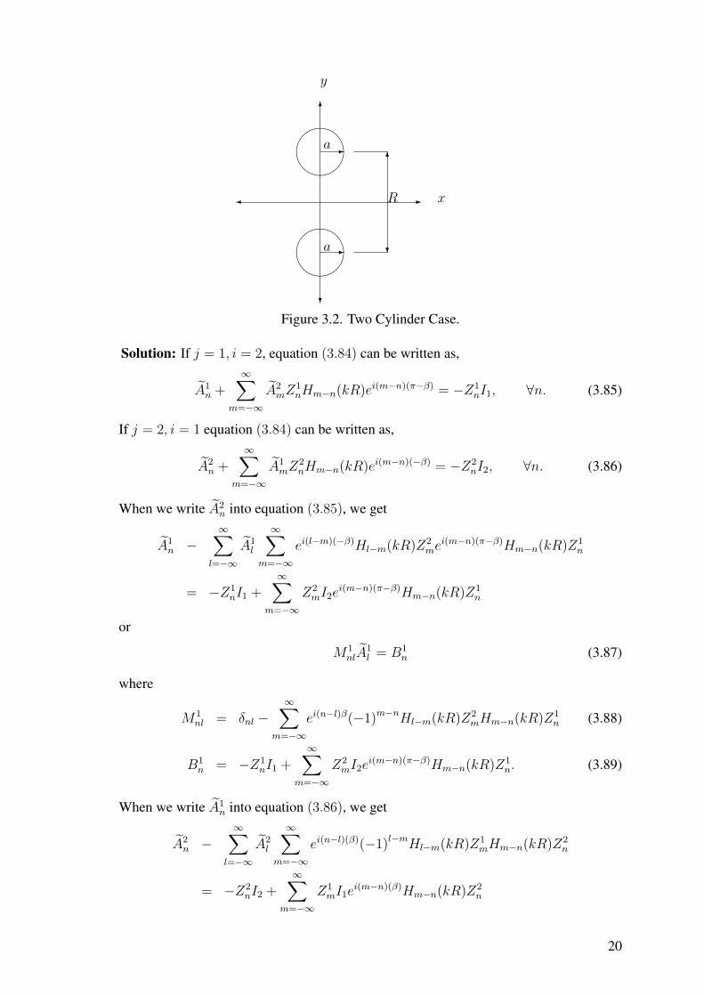
Example 3.3 ( Two Cylinder Case ) As an example we can consider two cylinder case:
center of first cylinder is at (0, R/2) and second one is at (0,−R/2). R is the distance
between the center of two cylinders, a is the radius of cylinders. α12 = −π/2, α21 = π/2.
(see Figure 2.2)
19
6
-
?
¾ x
y
&%
'$
&%
'$
-
-
a
a
6
?
R
Figure 3.2. Two Cylinder Case.
Solution: If j = 1, i = 2, equation (3.84) can be written as,
A1n +
∞∑m=−∞
A2mZ1
nHm−n(kR)ei(m−n)(π−β) = −Z1nI1, ∀n. (3.85)
If j = 2, i = 1 equation (3.84) can be written as,
A2n +
∞∑m=−∞
A1mZ2
nHm−n(kR)ei(m−n)(−β) = −Z2nI2, ∀n. (3.86)
When we write A2n into equation (3.85), we get
A1n −
∞∑
l=−∞A1
l
∞∑m=−∞
ei(l−m)(−β)Hl−m(kR)Z2mei(m−n)(π−β)Hm−n(kR)Z1
n
= −Z1nI1 +
∞∑m=−∞
Z2mI2e
i(m−n)(π−β)Hm−n(kR)Z1n
or
M1nlA
1l = B1
n (3.87)
where
M1nl = δnl −
∞∑m=−∞
ei(n−l)β(−1)m−nHl−m(kR)Z2mHm−n(kR)Z1
n (3.88)
B1n = −Z1
nI1 +∞∑
m=−∞Z2
mI2ei(m−n)(π−β)Hm−n(kR)Z1
n. (3.89)
When we write A1n into equation (3.86), we get
A2n −
∞∑
l=−∞A2
l
∞∑m=−∞
ei(n−l)(β)(−1)l−mHl−m(kR)Z1mHm−n(kR)Z2
n
= −Z2nI2 +
∞∑m=−∞
Z1mI1e
i(m−n)(β)Hm−n(kR)Z2n
20

or
M2nlA
2l = B2
n (3.90)
where
M2nl = δnl −
∞∑m=−∞
ei(n−l)β(−1)l−mHl−m(kR)Z1mHm−n(kR)Z2
n (3.91)
B2n = −Z2
nI2 +∞∑
m=−∞Z1
mI1ei(m−n)(β)Hm−n(kR)Z2
n. (3.92)
Let’s truncate the infinite series by taking l = 0 and n = 0,
M100A
1l = B1
0 (3.93)
M200A
2l = B2
0 (3.94)
where
M100 = M2
00 = 1−∞∑
m=−∞(−1)−mH−m(kR)Z1
mHm(kR)Z2n (3.95)
= 1−∞∑
m=−∞Hm
2(kR)Z1mZ2
0 (3.96)
B10 = −Z1
0I1 + Z10I2
∞∑m=−∞
Hm(kR)Z2meimβ
∼ −iπ(ak)2
4eikx1
2 sin β − iπ
8(ak)4eikx2
2 sin β ln(kR) +
−iπeikx22 sin β
∞∑m=1
(ak
2)m+2λm
m!((−1)me−imβ + eimβ).
B20 = −Z2
0I2 + Z20I1
∞∑m=−∞
Hm(kR)Z1meimβ
∼ −iπ(ak)2
4eikx2
2 sin β − iπ
8(ak)4eikx1
2 sin β ln(kR) +
−iπeikx12 sin β
∞∑m=1
(ak
2)m+2λm
m!(e−imβ + (−1)meimβ)
where λ = a/R.
By using limiting forms of the Bessel functions (see Appendix C) and taking the
leading order terms we get
A10 ∼ −i
π(ak)2
4eikx1
2 sin β + O(λ(ak)3) (3.97)
A20 ∼ −i
π(ak)2
4eikx2
2 sin β + O(λ(ak)3). (3.98)
21

Regardless of angle of attack β, modulus of A(j)0 is the same for both cylinders. Also, we
observe that λ does not appear in the first term, as obtained by (Linton and Evans 1990).
This suggests that in the limiting case, λ → 1/2, where the cylinders are almost touching,
there should be no convergence problem. Indeed, this is verified by the numerical calcu-
lations of the general problem (3.84) (Yılmaz 2004). In order to investigate the effect of
λ on convergence, we choose n = −1, 0, 1 and l = −1, 0, 1 in (3.88, 3.89 and 3.91, 3.92).
After some algebra we get,
A(2)−1 = i
π
4(ak)2(I2 + I1λ
2e−2iβ + I2λ4 + O(λ6))
A(2)0 = −i
π
4(ak)2I2
A(2)1 = i
π
4(ak)2(I2 + I1λ
2e2iβ + I2λ4 + O(λ6))
which means
A(2)−1 = i
π
4(ak)2(1 + λ2e−2iβe2ikb sin β + λ4 + O(λ6))
A(2)0 = −i
π
4(ak)2
A(2)1 = i
π
4(ak)2(1 + λ2e2iβe2ikb sin β + λ4 + O(λ6))
A(2)−1 = i
π
4(ak)2(1 + λ2e−2iβ + λ4 + O(λ6))
A(2)0 = −i
π
4(ak)2
A(2)1 = i
π
4(ak)2(1 + λ2e2iβ + λ4 + O(λ6))
where 2b = R. We see that the convergence is still unaffected by λ approaching the value
1/2.
22

CHAPTER 4
VORTEX-CYLINDER INTERACTION IN FLOWS
WITH NO FREE SURFACE
4.1. Complex Velocity
Let D be a region in the plane, the flow is incompressible , that is,
∂u
∂x+
∂v
∂y= 0 (4.1)
where V = (u, v) is velocity. Also assume that the flow is irrotational, that is,
∂u
∂y− ∂v
∂x= 0. (4.2)
Let
V = u− iv, (4.3)
which is called complex velocity, where V denotes complex conjugation. Equations (4.1)
and (4.2) are exactly the Caucy-Riemann equations for V , and so V is an analytic function
on D. The vector representing the complex velocity is the reflection, in the line through
the point considered parallel to the x-axis, of the vector of the actual velocity.
4.2. Complex Potential
If V has a primitive, V = dF/dz, then we call F the complex potential. Write
F = ϕ + iψ. Then (4.3) is equivalent to
u = ∂xϕ = ∂yψ and v = ∂yϕ = −∂yψ, (4.4)
that is, V = gradϕ and ψ is the stream function.
Conversely, if we assume for F any analytic function of z, the corresponding real
and imaginary parts give the velocity potential and stream of a possible two-dimensional
irrotational motion, for they satisfy (4.4) and Laplace equation.
23

4.2.1. Complex Potential for a Vortex
Complex potential for a vortex of strength κ at z0 is
ω = iκ log(z − z0).
4.2.2. Complex Velocity for a Vortex
Complex velocity for a vortex of strength κ at z0 is
Ω(z) =iκ
z − z0
. (4.5)
4.2.3. Streamlines of the Particle
A line drawn in the fluid so that its tangent at each point is in the direction of the
fluid velocity at that point is called a streamline. The stream function is constant along
the streamline. When the stream function is constant u = v = 0 and V = 0.
4.2.4. Boundary Conditions
As we analysed in Chapter 2, boundary condition, that the normal velocities are
both zero, or, the fluid velocity is everywhere tangential to the fixed surface. The boundary
of ck is given as a closed parametric curve
ck : z = z(t) = Zk(t), Zk(0) = Zk(2π), 0 ≤ t ≤ 2π,
(k=1,...,K). Then the tangent vector field to the curve ck is proportional to
T = Tx + iTy = z = Zk(t),
while the normal vector field is related to
n = nx + iny = iz = iZk(t).
On boundary ck, the normal component of the velocity field must be zero. This is equiva-
lent to the boundary condition
V n|ck= <(V n)|ck
=1
2(V n + V n)|ck
= 0.
24
or
Stream Function = Constant.
For the circle
ck : z(t) = zk + reit, 0 ≤ t ≤ 2π,
the tangent vector is
T = z = ireit = i(z(t)− zk),
the normal is
n = iz = −(z(t)− zk).
Then the boundary conditions are
[V (z)(z − zk) + V (z)(z − zk)
] |ck= 0, k = 1, ..., K.
4.3. Circle Theorem in Terms of Complex Velocity
Theorem 4.1 (The Circle Theorem) (Milne-Thomson 1960) Let there be irrotational
two-dimensional flow of incompressible inviscid fluid in the complex z plane. Let there be
no rigid boundaries and let the complex potential of the flow be F (z), where the singular-
ities of F (z) are all at the distance greater than a from the origin. If a circular cylinder,
typified by its cross-section the circle C, |z| = a, be introduced into the fluid of flow the
complex potential becomes
ω = F (z) + F (a2
z). (4.6)
Where F is complex conjugate.
Proof: Since z = a2/z on the circle, we see that ω as given by (4.6) is purely real on
the circle C and therefore stream function ψ = 0. Thus C is a streamline. If the point
z is outside C, the point a2/z is inside C, and vice-versa. Since all the singularities of
F (z) are by hypothesis exterior to C, all the singularities of F (a2
z) are interior to C; in
particular F (a2
z) has no singularity at infinity, since F (z) has none at z = 0. Thus ω has
exactly the same singularities as F (z) and so all the conditions are satisfied.¥
25

4.4. The Circle Theorem for Complex Velocity
Theorem 4.2 (The Circle Theorem for Complex Velocity) Let V (z) be complex ve-
locity, where V (z) = u − iv, in the infinite 2 − D flow. All singularities of V (z) are
outside r = a. When a cylinder of radius a is introduced at the origin, complex velocity
becomes:
Ω(z) = V (z)− a2
z2V (
a2
z). (4.7)
Proof : Boundary condition at r = a is that Ω(z)n must be zero. To show Ω(z)n = 0 on
the circle z = aeiθ, it is equivalent to show <Ω(z).eiθ = 0,
<Ω(z).eiθ = <[
V (z)− a2
z2V (
a2
z)
].eiθ
= <V (z).eiθ
−<
a2
z2V (
a2
z).eiθ
= <(u− iv)eiθ
−<(u + iv)e−iθ
= (u cos θ + v sin θ)− (u cos θ + v sin θ)
= 0.
This means Ω(z) satisfies the boundary condition.¥
Example 4.3 (Application of Theorem (4.2) for a Vortex of Strength κ)
Solution : Let us suppose that V (z) = iκz−z0
. Then,
Ω(z) =iκ
z − z0
− a2
z2
−iκa2
z− z0
(4.8)
Ω(z) = iκ1
z − z0
+ iκa2
z
1/z0
a2/z0 − z(4.9)
Ω(z) =iκ
z − z0
+iκ
z+
iκ
a2/z0 − z. (4.10)
To show <Ω(z).eiθ = 0 is equivalent to show Ωz + Ωz = 0.
z.Ω(z) = iκ
[z
z − z0
+ 1 +z0z
a2 − zz0
](4.11)
z.Ω(z) = −iκ
[z
z − z0
+ 1 +zz0
a2 − zz0
]. (4.12)
after the summation (4.11) and (4.12) and putting zz = a2 we get,
zΩ + zΩ = iκ
[z
z − z0
+zz0
a2 − zz0
− a2
a2 − z0z− z0
z − z0
]. (4.13)
After some algebraic manipulation, the right side of (4.13) vanishes.
26
4.4.1. Single Cylinder with a Vortex
1. A Vortex at z0 and a Cylinder at the Origin: For a vortex of strength κ at z0 and a
cylinder of radius a at the origin complex velocity as we found above,
Ω(z) =iκ
z − z0
+iκ
z+
iκ
a2/z0 − z. (4.14)
2. A Vortex at z0 and a Cylinder at z1,
Ω(z) =iκ
z − z0
− a2
(z − z1)2
−iκ
( a2
z−z1+ z1)− z0
=iκ
z − z0
+iκ
z − z1
+iκ
a2
z0−z1− (z − z1)
.
3. A Vortex at z0 and a Cylinder at zj ,
Ω(z) =iκ
z − z0
+iκ
z − zj
+iκ
a2
z0−zj− (z − zj)
. (4.15)
4.4.2. Multiple Cylinders with a Vortex
1. Laurent Series of iκz−z0
around zj ,
iκ
z − z0
= iκ
−(ξ0j)
−1 ∑∞n=0 (
ξj
ξ0j)n
if |ξj| < |ξ0j|(ξ0j)
−1 ∑∞n=0 (
ξ0j
ξj)n
if |ξ0j| < |ξj|.
2. Laurent Series of iκz−zj
+ iκa2
z0−zj−(z−zj)
around zj ,
= iκ
−
∞∑n=0
(a2/ξ0j)n+1
(ξj)n+2 if | ξj |<| ξ0j |
Where ξj = z − zj and ξ0j = z0 − zj.
4.4.3. Complex Velocity and Boundary Condition for Cylinder j
Total complex velocity around cylinder j is
V Tj = V I
j + V Dj +
n∑i=1i6=j
V Di (4.16)
=−iκ
ξ0j
∞∑n=0
(ξj
ξ0j
)n
+ iκ∞∑
n=0
Ajn
(ξ0j′)n+1
ξn+1j
(4.17)
+ iκ
n∑i=1i6=j
∞∑n=0
Ain
(ξ′0i)
n+1
(zj − zi + ξj)n+2. (4.18)
27

Boundary condition is
<V Tj .eiθj = 0, when | ξj |= aj.
Applying the boundary condition, unknown coefficients Ain can be found.
Changing coordinate system from (xi, yi) to (xj, yj): In equation (4.16) to write
Vi, we must change the coordinate system.
6
-
6
-
6
-
x
y
xi
yi
xj
yj
½¼
¾»½¼
¾»
³³³³³³³³³³³³1
¢¢¢¢¢¢¢¢¢¢¢
@@
@@
@@@I
ξi − ξj
ξi
ξj
z
ξi = z − zi
ξj = z − zj
ξi − ξj = zj − zi
Figure 4.1. Changing Coordinate System From ξi to ξj .
28

CHAPTER 5
VORTICES IN ANNULAR DOMAIN
5.1. Flow in Bounded Domain
Problem: Find complex velocity for incompressible irrotational flow in bounded
domain D. Where D is bounded by concentric circles. For multiply connected region
D with K islands of shapes c1, ..., cK , the complex velocity V = Vx − iVy is given by
Laurent series (see Appendix D)
V (z) = V0(z) +∞∑
n=0
anzn +
K∑α=1
∞∑n=0
bn+2
(z − zα)n+2
where points z1, ..., zK are inside of corresponding islands and V0(z) represents vortex
part.
5.2. N Vortices in Annular Domain
We consider problem of N point vortices in annular domain D : r1 ≤ |z| ≤ r2,
where z1, ..., zN are positions of vortices with strength κ1, ..., κN correspondingly. The
region is bounded by two concentric circles:
C1 : zz = r21
and
C2 : zz = r22.
(see Figure 4.1.)
Complex velocity is given by Laurent series (see Appendix D)
V (z) =N∑
k=1
iκk
z − zk
+∞∑
n=0
anzn +
∞∑n=0
bn+2
zn+2. (5.1)
29

¹¸
º·¹¸
º·
¹¸
º·
r
rr r r
rrrrr
rzN
z1
z2
cN
c1
c2
C1
−C2
?
¡¡¡ª
r2
r1
rI
j
I
I
I
Figure 5.1. N Vortices in Annular Domain.
5.2.1. Algebraic System for Boundary Value Problem
To find the unknown coefficients an, bn+2 we have to determine the boundary con-
ditions,
Γ = V (z)z + V (z)z (5.2)
=N∑
k=1
iκkz
z − zk
+∞∑
n=0
anzn+1 +
∞∑n=0
bn+2
zn+1
+N∑
k=1
−iκkz
z − zk
+∞∑
n=0
anzn+1 +
∞∑n=0
bn+2
zn+2. (5.3)
Since |zk| > |z| and zz = r12 on boundary C1, we rewrite equation (5.3) as follows;
N∑
k=1
iκkz
−zk
(1− z
zk
) +∞∑
n=0
anzn+1 +
∞∑n=0
bn+2
zn+1+ C.C. . (5.4)
using z = r21/z and expanding the first term in (5.4),
Γ|C1=
N∑
k=1
(−iκk)∞∑
n=0
(z
zk
)n+1
+∞∑
n=0
anzn+1 +
∞∑n=0
bn+2
zn+1
+N∑
k=1
iκk
∞∑n=0
(z
zk
)n+1
+∞∑
n=0
anzn+1 +∞∑
n=0
bn+2
zn+1(5.5)
=∞∑
n=0
[N∑
k=1
−iκk
zn+1k
+ an + bn+21
r2(n+1)1
]zn+1 + C.C. = 0, (5.6)
where C.C stands for complex conjugate. This implies the following algebraic systemN∑
k=1
−iκk
zn+1k
+ an + bn+21
r2(n+1)1
= 0, n = 0, 1, . . . (5.7)
30
Since |zk| < |z| and zz = r22 on boundary C2, we rewrite equation (5.3) as follows;
N∑
k=1
iκkz
z(1− zk
z
) +∞∑
n=0
anzn+1 +∞∑
n=0
bn+2
zn+1+ C.C. . (5.8)
Then, expanding the first term and using z = r22/z, we have
Γ|C2=
N∑
k=1
iκk
∞∑n=0
(zk
z
)n
+∞∑
n=0
anzn+1 +∞∑
n=0
bn+2
zn+1
+N∑
k=1
−iκk
∞∑n=0
( zk
z
)n
+∞∑
n=0
anzn+1 +
∞∑n=0
bn+2
zn+1(5.9)
=∞∑
n=0
[N∑
k=1
−iκkzn+1
k
r2(n+1)2
+ an + bn+21
r2(n+1)2
]zn+1 + C.C. = 0. (5.10)
This implies another algebraic system
N∑
k=1
−iκkzn+1k
r2(n+1)2
+ an + bn+21
r2(n+1)2
= 0, n = 0, 1, . . . (5.11)
5.2.2. Solution of Algebraic System
We have two sets of algebraic systems (5.7) and (5.11). By substracting (5.11)
from (5.7), we eliminate an
bn+2
[1
r2(n+1)2
− 1
r2(n+1)1
]+
N∑
k=1
(−iκk)
[zn+1
k
r2(n+1)2
− 1
zn+1k
]= 0. (5.12)
If q ≡ r22/r
21 we find,
bn+2 =N∑
k=1
(iκk
zn+1k
r2(n+1)2 − |zk|2(n+1)
qn+1 − 1
)(5.13)
bn+2 =N∑
k=1
(−iκk
zn+1k
r2(n+1)2 − |zk|2(n+1)
qn+1 − 1
)(5.14)
and from (5.7) we determine an,
an =N∑
k=1
iκk
zn+1k
− bn+21
r2(n+1)1
, (5.15)
or
an =N∑
k=1
−iκk
zn+1k
r2(n+1)1 − |zk|2(n+1)
r2(n+1)1 (qn+1 − 1)
. (5.16)
31
5.2.3. Solution in Terms of q-logarithmic Function
The Taylor series part of (5.1) gives the following,
∞∑n=0
anzn =∞∑
n=0
N∑
k=1
−iκk
zn+1k
zn
qn+1 − 1−
∞∑n=0
N∑
k=1
(−iκk)z(n+1)k zn
r2(n+1)1 (qn+1 − 1)
=N∑
k=1
iκk
zlnSZ
q
(1− z
zk
)−
N∑
k=1
iκk
zlnSZ
q
(1− zzk
r21
)(5.17)
and the Laurent part gives,
∞∑n=0
bn+2
zn+2=
N∑n=0
∞∑
k=1
−iκk
zn+1k
r2(n+1)2
(qn+1 − 1)
1
zn+2+
N∑n=0
∞∑
k=1
iκzn+1k
(qn+1 − 1)zn+2
=N∑
k=1
iκk
zlnSZ
q
(1− r2
2
zzk
)−
N∑
k=1
iκk
zlnSZ
q
(1− zk
z
)(5.18)
where lnSZq is q-logarithmic function given by the following definition.
Definition 5.1 (q-logarithmic function defined by series)
lnSZq (1 + x) =
∞∑n=1
(−1)n−1xn
qn − 1, |x| < q, q > 1. (5.19)
In the limiting case
limq→1
lnq(1 + x) = ln(1 + x). (5.20)
We will need the following lemma and its corollary later.
Lemma 5.1 Let q be real and q > 1. Then for all integers n ≥ 0 and k, with 0 < k <
qn+1, the following identity holds,
∞∑ν=n+1
1
qν + k=
1
klnSZ
q (1 +k
qn). (5.21)
Corollary 5.2 In the particular case when n = 0 from the lemma (5.1), we have a repre-
sentation of q-logarithm
lnSZq (1 + x) =
∞∑n=1
x
qn + x=
∞∑n=1
(−1)n−1xn
qn − 1(5.22)
or
lnq(1 + x) = (q − 1)∞∑
n=1
x
qn + x=
∞∑n=1
(−1)n−1xn
[n]. (5.23)
32
Proof: n = 0 in the lemma,
∞∑ν=1
1
qν + k=
1
klnSZ
q (1 + k). (5.24)
If n is replaced instead of ν
∞∑n=1
1
qn + k=
1
klnSZ
q (1 + k). (5.25)
substitute k = x ∞∑n=1
1
qn + x=
1
xlnSZ
q (1 + x). (5.26)
or
lnSZq (1 + x) =
∞∑n=1
x
qn + x=
∞∑n=1
(−1)n−1xn
qn − 1.¥ (5.27)
5.2.4. Complex Velocity and q-logarithm
Substituting equations (5.17) and (5.18) in (5.1) we get the following,
V (z) =N∑
k=1
iκk
z − zk
+N∑
k=1
iκk
zlnSZ
q
(1− z
zk
)−
N∑
k=1
iκk
zlnSZ
q
(1− zzk
r21
)
+N∑
k=1
iκk
zlnSZ
q
(1− r2
2
zzk
)−
N∑
k=1
iκk
zlnSZ
q
(1− zk
z
). (5.28)
Expanding q-log according to the Corollary (5.2) we have
V (z) =N∑
k=1
iκk
z − zk
+N∑
k=1
∞∑n=1
iκk
z − zkqn−
N∑
k=1
∞∑n=1
iκk
z − qn r21
zk
+N∑
k=1
∞∑n=1
iκk
z− iκk
z − q−n r22
zk
−
N∑
k=1
∞∑n=1
[iκk
z− iκk
z − q−nzk
]. (5.29)
V (z) =N∑
k=1
iκk
z − zk
+N∑
k=1
[ ∞∑n=1
iκk
z − zkqn+
∞∑n=1
iκk
z − zkq−n
],
−N∑
k=1
∞∑n=0
iκk
z − r21
zkq−n
+∞∑
n=0
iκk
z − r22
zkqn
. (5.30)
5.2.5. Vortex Image Representation
Equation (5.30) for complex velocity has countable infinite number of pole singu-
larities. These singularities can be interpreted as vortex images in two cylindrical surfaces.
33

For simplicity let us consider only one vortex at position z0, r1 < |z0| < r2. Then the set
of images in the cylinder C1 we denote z(1)I , z
(2)I , ... and in the cylinder C2 as z
(1)II , z
(2)II , ....
µ´¶³
r©
ª
©
ª
z0
r2r1
rz(2)Irz
(1)I rz
(2)IIrz
(1)II
− +−+ +©©*HHY
Figure 5.2. Vortex Image Representation.
Considering the above figure, we obtain the following,
z(1)I =
r21
z0
z(1)II =
r22
z0
(5.31)
z(2)I =
r21
z(1)II
=z0
qz
(2)II =
r22
z(1)I
= qz0 (5.32)
z(3)I =
r21
z(2)II
=r21
z0
1
qz
(3)II =
r22
z(2)I
=r22
z0
q (5.33)
z(4)I =
r21
z(3)II
=z0
q2z
(4)II =
r22
z(3)I
= z0q2 (5.34)
z(5)I =
r21
z(4)II
=r21
z0
1
q2z
(5)II =
r22
z(4)I
=r22
z0
q2. (5.35)
Combining together and taking into account alternating signs (positive for the first image
and negative for the next one - image of the image ) we have the set
+ z0, −z(1)I , +z
(2)II , −z
(3)I , +z
(4)II , −z
(5)I , ... (5.36)
and
+ z0, −z(1)II , +z
(2)I , −z
(3)II , +z
(4)I , −z
(5)II , .... (5.37)
This shows that the set of vortex images is completely determined by the singularities of
the q-logarithmic function.
34

5.3. Complex Potential and Elliptic Functions
In the above representation we can combine sums so that, we have
V (z) =N∑
k=1
[ ∞∑n=−∞
iκk
z − zkqn
]−
N∑
k=1
∞∑n=0
iκk
z − r21
zkq−n
+∞∑
n=1
iκk
z − r21
zkqn
(5.38)
=N∑
k=1
iκk
∞∑n=−∞
1
z − zkqn− 1
z − r21
zkqn
. (5.39)
Let us introduce the complex potential of the flow
V (z) = F ′(z)
so that by simple integration we get
F (z) =N∑
k=1
iκk
∞∑n=−∞
Ln
z − zkq
n
z − r21
zkqn
(5.40)
=N∑
k=1
iκkLn
∞∏n=−∞
z − zkqn
z − r21
zkqn
(5.41)
=N∑
k=1
iκkLn
z − zk
z − r21
zk
∞∏n=1
(z − zkqn)(z − zkq
−n)
(z − r21
zkqn)(z − r2
1
zkq−n)
. (5.42)
To compare our solution with that of Johnson and McDonald(2004), we consider one
vortex of strength κ at position z0,
F ′(z) = V (z) =∞∑
n=−∞
iκ
z − z0qn−
∞∑n=−∞
iκ
z − r21
z0qn
. (5.43)
Then for complex potential we have
F (z) = iκLn
∞∏n=−∞
(z − z0qn)
(z − r21
z0qn)︸ ︷︷ ︸
Φ
. (5.44)
For comparison purpose, we fix the radius r2 = 1 so that q =r22
r21
= 1r21≡ 1
q2 , where we
introduce new parameter q. Thus all singularities of F (z) are determined by zeroes and
poles of the function
Φ =∞∏
n=−∞
(z − z01
q2n )
(z − q2
z0
1q2n )
=∞∏
n=−∞
(z − z0q2n)
(z − 1z0
q2n)(5.45)
=z − z0
z − 1z0
∞∏n=1
(z − z0q2n)(z0 − zq2n)
(z − 1z0
q2n)( 1z0− zq2n)
. (5.46)
35

Ifz
z0
= e2iu, zz0 = e2iv, z0z0 =e2iv
e2iu(5.47)
we then obtain,
Φ =(1− e−2iu)
(1− e−2iv)
∞∏n=1
e2iv
e2iu
(1− q2ne2iu)(1− q2ne−2iu)
(1− q2ne2iv)(1− q2ne−2iv)(5.48)
Φ′ =2G
2G
q1/4 sin u
q1/4 sin v
∏∞n=1(1− q2ne2iu)(1− q2ne−2iu)∏∞n=1(1− q2ne2iv)(1− q2ne−2iv)
(5.49)
where Φ′ is a constant multiple of Φ,
G ≡∞∏
n=1
(1− q2n), q < 1, (5.50)
Φ′ =Θ1(u, q)
Θ1(v, q)=
Θ1(i2(τ − τ0), q)
Θ1(i2(τ + τ0), q)
(5.51)
where τ ≡ − ln z, τ0 ≡ − ln z0, τ0 ≡ − ln z0 and where Θ1 is the first Jacobi Theta
function (see Appendix D). (The last transformation is the conformal mapping of annular
domain to semi-infinite strip). Then
F (z) = iκLnΘ1(
i2(τ − τ0), q)
Θ1(i2(τ + τ0), q)
. (5.52)
For the stream function, we have
Ψ =F − F
2i=
iκ
2i
[Ln
Θ1
Θ1
+ LnΘ1
Θ1
](5.53)
= κLn
∣∣∣∣Θ1(
i2(τ − τ0), q)
Θ1(i2(τ + τ0), q)
∣∣∣∣ (5.54)
=−Γ
2πLn
∣∣∣∣Θ1(
i2(τ − τ0), q)
Θ1(i2(τ + τ0), q)
∣∣∣∣ (5.55)
This coincides with result of Johnson and McDonald (2004).
5.4. Motion of a Point Vortex in Annular Domain
We use the above formulas to determine the motion of single vortex in annular
domain. Complex velocity of vortex is determined by
z0 = x0 + iy0 = V (z)|z=z0 (5.56)
=∞∑
n=−∞
−iκ
z0 − z0qn−
∞∑n=−∞
−iκ
z0 − r21
z0qn
(5.57)
=−iκ
z0
∞∑n=−∞
1
1− qn+ z0iκ
∞∑n=−∞
1
|z0|2 − r21q
n. (5.58)
36

Substituting this to following equation we have,
z0z0 + z0 ˙z0 =d
dt|z0|2 = 0 → |z0| = constant. (5.59)
This implies that the distance of the vortex from the origin is constant. Then only the
argument is time independent,
z0 = |z0|eiϕ(t), z0 = z0eiϕiϕ, (5.60)
which satisfies
ϕ = −κ
[1
|z0|2∞∑
n=−∞
1
1− qn−
∞∑n=−∞
1
|z0|2 − r21q
n
]. (5.61)
The right hand side of equation 5.61 is a constant and the solution is
ϕ(t) = ωt + ϕ0 (5.62)
where frequency ω is dependent on modulus |z0|,
ω = −κ
[1
|z0|2∞∑
n=−∞
1
1− qn−
∞∑n=−∞
1
|z0|2 − r21q
n
](5.63)
=−κ
|z0|2∞∑
n=0
1
qn+1 − 1
[( |z0|2r21
)n+1
−(
r22
|z0|2)n+1
]. (5.64)
Finally solution of our problem can be written by using q-logarithmic function
ω =κ
|z0|2(q − 1)
[lnq
(1− |z0|2
r21
)− lnq
(1− r2
2
|z0|2)]
. (5.65)
So, we found that vortex is uniformly rotating around the center,
z0(t) = |z0|eiωt+iϕ0 = z0(0)eiωt (5.66)
with frequency depending on vortex strength, initial position and geometry of annular
domain in terms of q-logarithms. This reflects the fact that the motion of vortex results
from interaction with infinite set of its images in the cylinders.
37

CHAPTER 6
CONFORMAL MAPPING OF ANNULAR DOMAIN
ONTO
THE INFINITE DOMAIN WITH TWO CYLINDERS
6.1. Mobius Transformation and Mappings of the Annular Domain
Definition 6.1 A mapping of the form
t(z) =az + b
cz + d(6.1)
where a, b, c, d ∈ C, is called a linear fractional transformation. If a, b, c and d also
satisfy ad− bc 6= 0 then t(z) is called Mobius transformation. (Churcill and Brown 1984)
when c 6= 0, equation (6.1) can be written
w =a
c+
bc− ad
c
1
cz + d; (6.2)
and it is clear how the condition ad−bc 6= 0 ensures that a linear fractional transformation
is never a constant function.
If c = 0 (d 6= 0), then t(z) in equation (6.1) reduces to the entire linear transfor-
mation,
t(z) = αz + β,
(α =
a
d, β =
b
d
)(6.3)
Mobius transformations carries generalized circles into generalized circles. In the ex-
tended plane a generalized circle is either a circle or a straight line (Circle with infinite
radius).
6.1.1. Equation of Circle
Let c ∈ C, ρ > 0 and Γ be the circle with center c and radius ρ, then the equation
of the circle
(z − c)(z − c) = ρ2. (6.4)
38
6.1.2. Symmetry with Respect to Circle
Definition 6.2 If
(z1 − c)(z2 − c) = ρ2 (6.5)
then z1 and z2 are symmetric with respect to Γ.
Lemma 6.1 If a and b are complex numbers, µ > 0∣∣∣∣z − a
z − b
∣∣∣∣ = µ (6.6)
represents a generalized circle. Number µ is related with the circle radius ρ, ρ = µ|a−b|(1−µ2)
.
Equation (6.6) becomes a straight line if and only if µ = 1.
Proof : First of all lets show that equation (6.6) is a circle. Expansion of |z − c|2 = ρ2
gives the following,
zz − cz − cz + cc− ρ2 = 0 (6.7)
On the other hand, expansion of (6.6) yields,
(1− µ2)zz + (µ2b− a)z + (µ2b− a)z + (aa− µ2bb) = 0 (6.8)
zz +(µ2b− a)
(1− µ2)z +
(µ2b− a)
(1− µ2)z +
(aa− µ2bb)
1− µ2= 0 (6.9)
If we compare equation (6.9) with equation (6.7), we find, c = (a−µ2b)(1−µ2)
and ρ2 =
µ2(a−b)(a−b)(1−µ2)2
. This implies that (6.6) represents a circle.
If generalized circle represents a straight line then we will show µ = 1. For the general-
ized circle in equation (6.8) to be a straight line, the coefficient of zz must be zero. This
means 1 − µ2 = 0, then since µ > 0, we get µ = 1. If we substitute µ = 1 in equation
(6.6)
|z − a| = |z − b| (6.10)
(z − a)(z − a) = (z − b)(z − b) (6.11)
(b− a)z + (b− a)z + aa− bb = 0 (6.12)
since the last equation is in the form Az + Az + C = 0, which is equation of a line, we
get the desired result.¥
Theorem 6.2 The points a and b are symmetric with respect to the generalized circle
(6.6).
39

Proof : If a and b are symmetric point, from equation (6.5) we should have
(a− c)(b− c) = ρ2. (6.13)
If we substitute c = (a−µ2b)(1−µ2)
and ρ2 = µ2(a−b)(a−b)(1−µ2)2
in equation (6.13), then we get(
a− a− µ2b
1− µ2
)(b− a− µ2b
(1− µ2)
)=
µ2(b− a)
1− µ2.b− a
1− µ2(6.14)
= ρ2. (6.15)
Hence equation (6.13) is satisfied.¥
Theorem 6.3 Let a and b be symmetric with respect to generalized circle Γ, a 6= b, then
∃ µ > 0 such that Γ is given by equation (6.6)
Proof : Since a and b are symmetric we can write
(a− c)(b− c) = ρ2 (6.16)
ab− ac− cb = ρ2 − cc. (6.17)
Equation of a circle with center c and radius ρ is
(z − c)(z − c) = ρ2 (6.18)
zz − cz − cz + cc = ρ2. (6.19)
In the last equation, (ρ2 − cc), can be replaced by(6.17) and using c = (a−µ2b)(1−µ2)
, we get
zz − (a− µ2b)
(1− µ2)z − (a− µ2b)
(1− µ2)z = ab− a
(a− µ2b)
(1− µ2)− (a− µ2b)
(1− µ2)b (6.20)
zz − µ2zz − az + µ2bz − az + µ2bz = µ2bb− aa (6.21)zz − az − az + aa
bb + zz − bz − bz= µ2 (6.22)
∣∣∣∣z − a
z − b
∣∣∣∣ = µ.¥ (6.23)
Theorem 6.4 Let a and b be two points of the complex plane which are symmetric with
respect to generalized circle Γ and let t be a Mobius transformation, then a′ = t(a) and
b′ = t(b) are symmetric with respect to Γ′,where Γ′ is the image of Γ under t.
Proof : If
t(z) = z + m, t is translation; (6.24)
t(z) = mz, m > 0, t is a dilation; (6.25)
t(z) = eiθz, t is rotation; (6.26)
t(z) = 1/z, t is inversion. (6.27)
40

Mobius transformation is a composition of translation, rotation, inversion and dilation.
When the circle is translated, rotated and dilated, its symmetry is conserved. So it is
sufficient to consider the inversion only, t(z) = 1/z. Since a and b are inverses of each
other with respect to the circle Γ by Theorem 6.3 equation for Γ is,∣∣∣∣z − a
z − b
∣∣∣∣ = µ for some µ. (6.28)
Applying inversion (z = 1/w) to t, we have,∣∣∣∣
1w− a
1w− b
∣∣∣∣ = µ (6.29)∣∣∣∣w − a′
w − b′
∣∣∣∣ = µ
∣∣∣∣b
a
∣∣∣∣ , where,1
a= a′,
1
b= b′. (6.30)
This shows that a′ and b′ are symmetric with respect to Γ′.¥
6.1.3. Mapping of Disc onto Unit Disc
Example 6.5 Let D be a disk and let a be a point in D. Find all Mobius transformations
t which maps D onto the unit disc such that t(a) = 0.
6
-
?
¾ x
y
&%
'$a
D
.
D′
-t 6
-
?
¾ u
v
&%
'$
1
Figure 6.1. Mapping of D onto Unit Disc.
Solution : We have two cases,
1) If a is the center of D, by using the entire Mobius transformation t = az + b we can do
the mapping.
2) If a is not the center, we can use Mobius transformation
t = cz − a
z − b, (6.31)
where b is the inverse of a, then ab = 1, a 6= b.
Let us take any point z1 on the boundary of D,
z1′ = c
z1 − a
z1 − b
41

since z1′ is on the unit circle then
|cz1 − a
z1 − b| = 1
then |c| = | z1−bz1−a
| and c = |c|eiα, 0 < α < 2π. Mobius transformation for this case is
t = eiα
∣∣∣∣z1 − b
z1 − a
∣∣∣∣z − a
z − b, 0 < α < 2π. (6.32)
6.1.4. Mapping of Unit Disc onto Unit Disc
Example 6.6 Find the most general Mobius transformation t such that it maps unit disk
onto itself.
6
-
?
¾ x
y
&%
'$a
D.
D′
-t 6
-
?
¾ u
v
&%
'$
1
Figure 6.2. Mapping of Unit Disc onto Unit Disc.
Solution : This example is a special case of the previous example. Since D is unit disk
we can take z1 = 1, in (6.32),
t(z) = eiα′ z − a
1− az(6.33)
where∣∣ a−11−a
∣∣ = 1 and eiα′ = eiα. a|a| .
Example 6.7 Let c and ρ be real and c > ρ > b. Map the domain by |z − c| ≤ ρ and
left hand side of the imaginary axis onto an annular domain bounded by |w| = 1 and a
concentric circle. Find the Mobius transformation.
6
-
?
¾ x
y
&%
'$acb
q
-t6
-
?
¾ u
v
m1
&%
'$q q
¡¡¡¡¡¡¡¡¡¡¡¡¡¡
¡¡
¡¡¡
¡¡
¡
¡¡¡
¡¡
¡¡
¡¡¡¡
¡¡¡¡
Figure 6.3. Mapping of Given D onto Annular Domain.
42

Solution : In this example a and b are symmetric with respect to y-axis and |z −c| = ρ2. Since a and b are symmetric with respect to y-axis then
b = −a.
Since they are symmetric with respect to |z − c| = ρ2 they must satisfy
(b− c)(a− c) = ρ2.
If we replace b = −a, we can find
a = (c2 − ρ2)1/2
b = −(c2 − ρ2)1/2.
Mobius transformation is
t(z) =z − (c2 − ρ2)1/2
z + (c2 − ρ2)1/2. (6.34)
Example 6.8 Let ρ and c be real and, 0 < c < 1 − ρ. Map the domain bounded by the
circles |z| = 1 and |z − c| = ρ onto domain bounded by two concentric circles such that
the outer circle is mapped onto itself. What is the radius R0 of the inner circle?
Solution : Using the symmetry of a and b with respect to unit circle and |z − c| = ρ we
can find
a =1 + c2 − ρ2 +
√(1− (c + ρ)2)(1− (c− ρ)2)
2c(6.35)
b =2c
1 + c2 − ρ2 +√
(1 + c2 − ρ2)2 − 4c2. (6.36)
and Mobius transformation;
t(z) = w =z − a
az − 1(6.37)
To find R0 we can substitute z = c− ρ in (6.37), then
R0 =1− c2 + ρ2 +
√(1− (c + ρ)2)(1− (c− ρ)2)
2ρ(6.38)
If c = x1+x2
2and ρ = x1−x2
2, we get same result with that of Churchill and Brow(Churchill
and Brow 1984).
43
6.1.5. Mapping of Two Cylinder onto Annular Domain
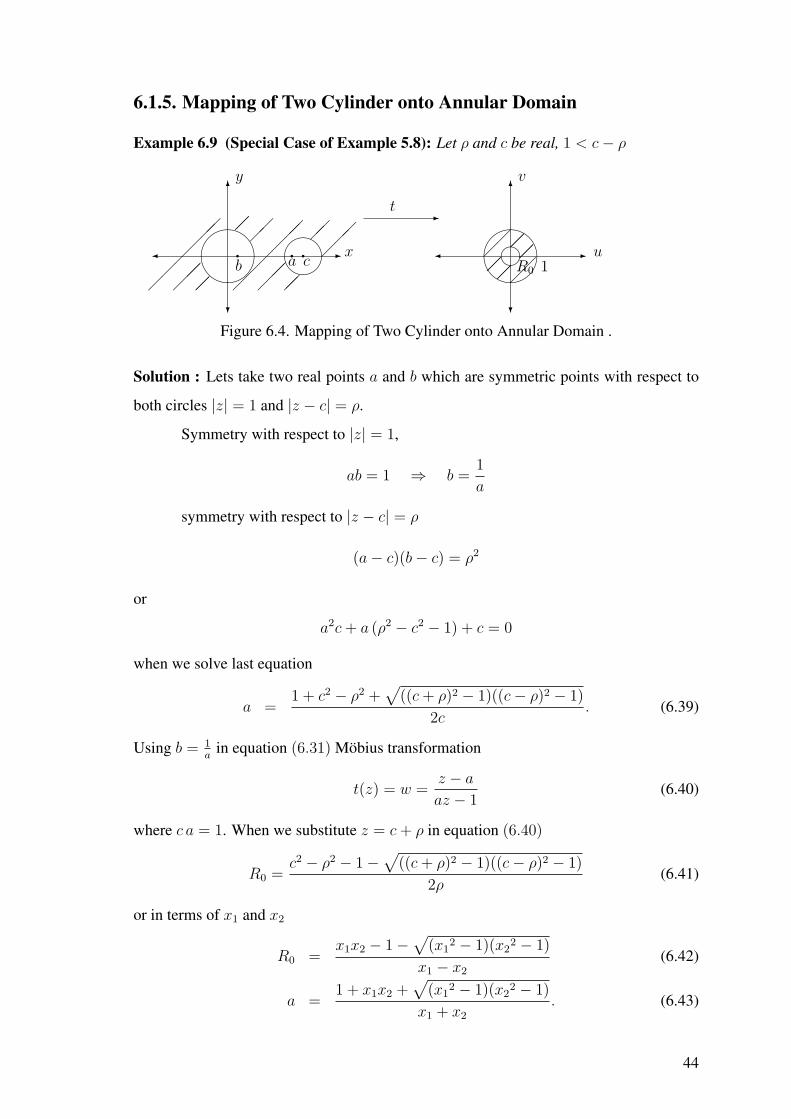
Example 6.9 (Special Case of Example 5.8): Let ρ and c be real, 1 < c− ρ
6
-
?
¾ x
y
½¼
¾»
&%
'$
b caq qq
-t6
-
?
¾ u
v
R0
m1
&%
'$¡
¡
¡¡
¡¡¡¡
¡¡¡¡
¡¡
¡¡
¡¡
¡¡¡
¡¡¡
¡
¡¡ ¡¡
¡¡
¡¡
¡¡¡
¡¡
¡¡¡
¡¡
Figure 6.4. Mapping of Two Cylinder onto Annular Domain .
Solution : Lets take two real points a and b which are symmetric points with respect to
both circles |z| = 1 and |z − c| = ρ.
Symmetry with respect to |z| = 1,
ab = 1 ⇒ b =1
a
symmetry with respect to |z − c| = ρ
(a− c)(b− c) = ρ2
or
a2c + a (ρ2 − c2 − 1) + c = 0
when we solve last equation
a =1 + c2 − ρ2 +
√((c + ρ)2 − 1)((c− ρ)2 − 1)
2c. (6.39)
Using b = 1a
in equation (6.31) Mobius transformation
t(z) = w =z − a
az − 1(6.40)
where c a = 1. When we substitute z = c + ρ in equation (6.40)
R0 =c2 − ρ2 − 1−
√((c + ρ)2 − 1)((c− ρ)2 − 1)
2ρ(6.41)
or in terms of x1 and x2
R0 =x1x2 − 1−
√(x1
2 − 1)(x22 − 1)
x1 − x2
(6.42)
a =1 + x1x2 +
√(x1
2 − 1)(x22 − 1)
x1 + x2
. (6.43)
44

6.2. Application of the Mobius Transformation to the Vortex-Cylinder
Problem
Let assume that there exist a vortex at z0 in infinite domain (see Figure(6.8)), then
the image of complex potential in w-plane is,
F (z) = ln(z − z0) (6.44)
F (z(w)) = f(w) = ln
(w − a
aw − 1− w0 − a
aw0 − 1
)(6.45)
= ln
(a2 − 1
a(aw0 − 1)
)+ ln(w − w0)− ln(w − 1
a), (6.46)
where w0 is the image of the point z0. Hence if there exists a vortex z0 in z-plane then its
image vortices with opposite strength are at w0 and 1/a. In Chapter 4, we found vortex
image representation for N vortices in annular domain (See equation (5.40)). Now we
consider 2 vortices at positions w0 and 1a,
f(w) =2∑
k=1
iκk
∞∑n=−∞
Ln
w − wkq
n
w − r21
wkqn
(6.47)
= iκ
∞∑n=−∞
Ln
(w − w0q
n
w − R20
w0qn
)− iκ
∞∑n=−∞
Ln
(w − qn
a
w − aR02qn
)(6.48)
= iκ
∞∑n=−∞
Ln
(w − w0q
n
w − R20
w0qn
.w − aR2
0qn
w − qn
a
). (6.49)
where r1 = R0, r2 = 1 and q ≡ 1R2
0.
By applying the inverse mapping w = z−aaz−1
, we can find its vortex image repre-
sentation in z-plane,
F (z) = iκ
∞∑n=−∞
Ln
αn
z + w0qn−a1−aw0qn
z +R2
0qn−aw0
w0−aR20qn
.z +
−a+aR20qn
1−a2R20qn
z + qn−a2
a−aqn
(6.50)
= iκ
∞∑n=−∞
Ln
(αn
z − t(w0qn)
z − t(R2
0qn
w0)
.z − t(aqnR2
0)
z − t( qn
a)
)(6.51)
where αn =(1−aw0qn)(1−a2R2
0qn)
(w0−aR20qn)(a−aqn)
.
By differentiating the equation (6.51), we can write the corresponding complex velocity
as,
V (z) = iκ
∞∑n=−∞
(1
z − t(w0qn)+
1
z − t(aqnR20)− 1
z − t(R2
0qn
w0)− 1
z − t( qn
a)
). (6.52)
45
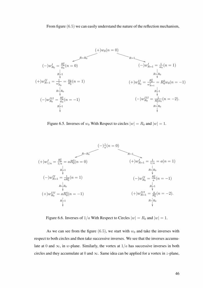
From figure (6.5) we can easily understand the nature of the reflection mechanism,
(+)w0(n = 0)
R=R0jjjjjjj
ttjjjjj R=1UUUUUUUU
**UUUUUUU
(−)wIR0
=R2
0
w0(n = 0)
R=1²²
(−)wIR=1 = 1
w0(n = 1)
R=R0
²²(+)wII
R=1 = 1¯wIR0
= w0
R20(n = 1)
R=R0
²²
(+)wIIR0
=R2
0¯wI
R=1
= R20w0(n = −1)
R=1
²²
(−)wIIIR0
=R4
0
w0(n = −1)
R=1
²²
(−)wIIIR0
= 1R2
0w0(n = −2).
R=R0
²²
Figure 6.5. Inverses of w0 With Respect to circles |w| = R0 and |w| = 1.
(−) 1a(n = 0)
R=R0jjjjjjj
uujjjjj R=1TTTTTTT
))TTTTTT
(+)wI1/a =
R20
1/a= aR2
0(n = 0)
R=1²²
(+)wIR=1 = 1
1/a= a(n = 1)
R=R0
²²(−)wII
R=1 = 1aR2
0(n = 1)
R=R0
²²
(−)wIIR0
=R2
0
a(n = −1)
R=1²²
(+)wIIIR0
= aR40(n = −1)
R=1
²²
(+)wIIIR=1 = a
R20(n = −2).
R=R0
²²
Figure 6.6. Inverses of 1/a With Respect to Circles |w| = R0 and |w| = 1.
As we can see from the figure (6.5), we start with w0 and take the inverses with
respect to both circles and then take successive inverses. We see that the inverses accumu-
late at 0 and ∞, in w-plane. Similarly, the vortex at 1/a has successive inverses in both
circles and they accumulate at 0 and∞. Same idea can be applied for a vortex in z-plane,
46

(−)z0(n = 0)
R=ρjjjjjjj
ttjjjjjj R=1UUUUUUU
**UUUUUU
(+)zIρ = ρ2
z0−c+ c(n = 0)
R=1²²
(+)zIR=1 = 1
z0(n = 1)
R=ρ²²
(−)zIIR=1 = 1
zIρ(n = 1)
R=ρ
²²
(−)zIIρ = ρ2
zIR=1−c
+ c(n = −1)
R=1²²
(+)wIIIρ = ρ2
zIIR=1
+ c(n = −1)
R=1
²²
(+)wIIIR=1 = 1
zIIR0
(n = −2)
R=ρ
²²
Figure 6.7. Inverses of z0 With Respect to Circles |z| = 1 and |z − c| = ρ.
We notice that inverses in z-plane accumulate at a and 1/a.
Example 6.10 In order to visualize the images, we consider a numerical example;
x1 = 4, x2 = 2 and w0 = 0.5i + 0.5.
6
-
?
¾ u
v
q
1a
w0
1R0
-t
6
-
?
¾ x
y
1 x2 x1c
z0
&%
'$
q
&%
'$qqp pp pp pp ppppp p p
p pp pp pp pp pp pp p1a
a
p
p
p
p
p
p
p
p
pppp
Figure 6.8. Vortex Image Approximation.
We calculate that a = 2.61803 and R0 = 0.145898.
47

Vortex at w0
w0 = 0.5 + 0.5i
ttiiiiiiiiiiiiiiiii
**UUUUUUUUUUUUUUUU
wIR0
= 0.2 + 0.2i
,,ZZZZZZZZZZZZZZZZZZZZZZZZZZZZZZZZZZZZ wIR=1 = 1 + i
rrddddddddddddddddddddddddddddddddddddd
wIIR=1 = 23.4 + 23.4i
,,ZZZZZZZZZZZZZZZZZZZZZZZZZZZZZZZZZwII
R0= 0.01 + 0.01i
rrdddddddddddddddddddddddddddddddd
wIIIR0
= 4x10⁻⁴ + 4x10⁻⁴i
,,ZZZZZZZZZZZZZZZZZZZZZZZZZZZZZZwI
R=1 = 46.9 + 46.9i
rrdddddddddddddddddddddddddddddddd
wIVR=1 = 1103 + 1103i
,,ZZZZZZZZZZZZZZZZZZZZZZZZZZZZZZZZwI
R0= 0.0002 + 0.0002i
rrdddddddddddddddddddddddddddddd
wVR0
= 9.6x10⁻⁶ + 9.6x10⁻⁶i wVR=1 = 2207 + 2207i
Vortex at 1/a
1/a = 0.3819
vvmmmmmmmmmmmm
((QQQQQQQQQQQQQ
wI1/a = 0.05
++XXXXXXXXXXXXXXXXXXXXXXXXXXX wIR=1 = 2.6
ssffffffffffffffffffffffffffff
wI1/a = 17.9
++XXXXXXXXXXXXXXXXXXXXXXXXXXXX wIR=1 = 0.008
ssffffffffffffffffffffffffff
wI1/a = 10−3
++XXXXXXXXXXXXXXXXXXXXXXXXXXX wIR=1 = 122
ssffffffffffffffffffffffffffff
wI1/a = 842
++XXXXXXXXXXXXXXXXXXXXXXXXXXX wIR=1 = 10−4
ssffffffffffffffffffffffffff
wI1/a = 2x10⁻⁵ wI
R=1 = 5778
Figure 6.9. Images of w0 and 1/a.
From the calculations we can see that images of both vortices accumulate at zero and
infinity in w-plane. When we map the annular domain onto z-plane, there exist a vortex
at z0 and images of this vortex converge to a and 1/a as you see below,
48

z0 = −4.805× 10⁻¹⁷ + 1.6180i
R=ρggggggggg
ssgggggggg R=1WWWWWWWWW
++WWWWWWWW
zIρ = 2.74 + 0.139i
--[[[[[[[[[[[[[[[[[[[[[[[[[[[[[[[[[[[[[[[[[[[[[[[ zIR=1 = −10−17 + 0.6i
qqcccccccccccccccccccccccccccccccccccccccccccc
zIIR=1 = 0.36 + 0.01i
--[[[[[[[[[[[[[[[[[[[[[[[[[[[[[[[[[[[[[[[[[[[[ zIIρ = 2.68 + 0.06i
qqcccccccccccccccccccccccccccccccccccccccccccccc
zIIIρ = 2.62 + 0.002i
--[[[[[[[[[[[[[[[[[[[[[[[[[[[[[[[[[[[[[[[[[[[[[ zIIIR=1 = 0.37 + 0.009i
qqccccccccccccccccccccccccccccccccccccccccccc
zIVR=1 = 0.38 + 0.0003i
--[[[[[[[[[[[[[[[[[[[[[[[[[[[[[[[[[[[[[[[[[[[ zIVR0
= 2.61 + 0.001i
qqcccccccccccccccccccccccccccccccccccccccccccc
zVρ = 2.61 + 0.00005i zV
R=1 = 0.38 + 0.0001i
Figure 6.10. Images of z0.
49

CHAPTER 7
CONCLUSION
Scattering of water waves and its long wave approximation and vortex-cylinder
interaction were studied.
In the first part, starting from mathematical formulation of the water-wave prob-
lem we solved truncated system for velocity potential with unknown coefficients. In the
limiting case which is known as Long-Wave approximation we found unknown coeffi-
cients; A10 and A2
0 behaves like O((ak)2) as k → 0. Also A11, A
1−1, A
21 and A2
−1 behave
like O((ak)2) as k → 0.
In the second part we tried to do the same thing for vortex-cylinder case by using
the Circle Theorem. To apply boundary condition Laurent series expansion was neces-
sary. This problem needs further attention.
Finally, complex velocity and potential in annular domain are obtained using com-
plex analysis and q-logarithm. By using conformal mapping, annular domain is mapped
onto the infinite 2−D plane with two circular cylinders. Solution in both domains involve
the inverse images in both cylinders. Image representation is clearly depicted.
50
REFERENCES
Abromowitz, M. and Stegun, I.A., 1965. Handbook of Mathematical Functions, (Dower,NewYork).
Cagatay, F., Gurkan, Z.N., Pashaev, O. and Yilmaz, O. Tubitak Projesi (106T447), 1. Ge-lisme Raporu, 2007.
Chorin, A.J. and Marsden, J.E., 1992. A Mathematical Introduction to Fluid Mechanics,(Springer-Verlag, New York), pp.1-21.
Churcill, R.V. and Brown, J.W., 1984. Complex Variables and Applications, (McGraw-Hill), p.328.
Crapper, G. D., 1984. Introduction to Water Waves, (Ellis Horwood, Chichester).
Gurkan, Z.N. and Pashaev, O., 2007. “ Integrable Vortex Dynamics in Anisotropic PlanarSpin Liquid Models ”, Chaos, Solıtonts and Fractals doi: 10. 1016/ j. chaos. 2006.11. 013, (In Press).
Haskind, M. D(Khaskind) 1973. The Hydrodynamic Theory of Ship Oscillations, (Nauka,Moscow).
Johnson, E.R. and McDonald, N.R., 2004. “ The Motion of a Vortex Near Two CircularCylinders ”, Proc. R. Soc. London A, p.460, 939-54.
Kaplan W., 1959. Advanced Calculus, (Addison-Wesley Publishing Company), p.329.
Kuznetsov, N., Maz’ya, V. and Vainberg, B.,2007. Linear Water Waves A MathematicalApproach, (Cambridge University Press, United Kingdom).
Lamb, H., 1932. Hydrodynamics, (Cambridge University Press).
Lighthill, M.J., 1978. Waves in Fluids, (Cambridge University Press).
Linton, C.M. and Evans, D.V., 1990. “ The Interaction of Waves with Arrays of VerticalCircular Cylinder”, J. Fluid Mech.,p.215, 549-69.
Linton C.M and McIver, P., 2001. Handbook of Mathematical Techniques for Wave Structure Interactions, (CRC Press, Boca Raton).
Mei, C.C., 1983. The Applied Dynamics of Ocean Surface Waves, (Wiley, New York).
Milne-Thomson L.M., 1960. Theoretical Hydrodynamics, (The Macmillan Company,New York), p.154.
Newman, J.N., 1977.Marine Hydrodynamics, (MIT Press, Cambridge).
Newman, J.N., 1978. “ The Theory of Ship Motions ”, Adv.Appl.Mech. 18 pp.221-283.
Pashaev, O.K. and Gurkan, Z.N., 2007. “Abelian Chern- Simons Vortices and Holomorphic Burger’s Hierarchy”, Theor. Math. Phys.(In Press ).
51
Spring, B.H. and Monkmeyer, P.L., 1974. “Interaction of Plane Waves with VerticalCylinders”, Proc. 14th Intl Conf. on Coastal Engineering Chap. p.107, 1828-45.
Sretnsky, L.N., 1977. The Theory of Wave Motions of a Fluid, (Nauka, Moscow).
Stoker, J.J., 1957. Water Waves. The Mathematical Theory with Applcations (Interscience,New York).
Wehausen, J.V. 1971. “The Motion of Floating Bodies” Ann.Rev.Fluid Mec.3, pp.237-268.
Wehausen, J.V. and Laitone, E.V., 1960.“ Surface Waves”, Handbuch der Physik9(Springer-Verlag, Berlin), pp. 446-778.
Whitham, G.B., 1979. Lectures on Wave Propagation, (Springer, New York).
Whittaker, E.T. and Watson G.N., 1969. A Course of Modern Analysis, (Cambridge).p.470
Yılmaz, O., 2004. “An Iterative Procedure for the Diffraction of Water Waves by MultipleCylinders”, Ocean Engineering, 31, 1437-46.
52

APPENDIX A
DIVERGENCE THEOREM
A.1. Divergence Theorem
Theorem A.1 (Divergence Theorem) ( Kaplan Wilfred 1959) Let v = Li + M j + Nk
be a vector field in a domain D of space; let D,M, N be continuous and have continuous
derivatives in D. Let S be a piecewise smooth surface in D that forms the complete
boundary of a bounded closed region R in D. Let n be the outer normal of S with respect
to R. Then ∫
S
∫vndσ =
∫ ∫
R
∫divv dxdydz; (A.1)
that is,∫
S
∫Ldydz + Mdzdx + Ndxdy =
∫ ∫
R
∫ (∂L
∂x+
∂M
∂y+
∂N
∂z
). (A.2)
53

APPENDIX B
SEPARATION OF VARIABLES
B.1. Solution of No Body Problem Using Separation of Variables
Problem
∇2φ = 0 in W, (B.1)
φy − νφ = 0 on F (on y = 0), (B.2)
∂φ
∂y= 0 on B (on y = −d). (B.3)
Solution: If we replace φ = G(x1)H(x2)Y (y) into equation (B.1) and dividing
by G(x1)H(x2)Y (y) we get,
Gx1x1
G+
Hx2x2
H+
Yyy
Y= 0. (B.4)
or equivalently
Gx1x1
G=−Hx2x2
H+−Yyy
Y= −k2
1 (B.5)
(B.6)
which means
Gx1x1 + k21G = 0 (B.7)
Hx2x2
H+
Yyy
Y= k2
1 (B.8)
if second separation is done to last equation
Hx2x2 + k22H = 0 (B.9)
Yyy − (k21 + k2
2)Y = 0 (B.10)
for some constant k2. From the solution of equations (B.7), (B.9) and (B.10) we get,
G(x1) = c1eik1x1 + c2e
−ik1x1 (B.11)
H(x2) = c3eik2x2 + c4e
−ik2x2 (B.12)
Y (y) = c5 cosh(√
k21 + k2
2)y + c6 sinh(√
k21 + k2
2)y (B.13)
54

If the boundary condition (B.3) is applied to the equation (B.13)
Y (y) = c5 (cosh(ky) + tanh(kd) sinh(hy)) (B.14)
where k =√
k21 + k2
2
φ = Y (y)G(x1)H(x2)
= c5 (cosh(ky) + tanh(kd) sinh(hy))(c1e
ik1x1 + c2e−ik1x1
) (c3e
ik2x2 + c4e−ik2x2
)
= c5 (cosh(ky) + tanh(kd) sinh(hy))(c1e
ik1x1+ik2x2 + c2e−ik1x1−ik2x2
)
=cosh k(y + d)
cosh(kd)(c1eik.x + c2e−ik.x)
where c1 = c5.c1, c2 = c5.c2 and k.x = k1x1 + k2x2.
Velocity potential
φ1 = Re
cosh k(y + d)
cosh(kd)(c1eik.x−iωt + c2e−ik.x−iωt)
. (B.15)
55

APPENDIX C
BESSEL FUNCTIONS
C.1. Bessel’s Differential Equation
x2d2w
dz2+ z
dw
dz+ (z2 − ν2)w = 0 (C.1)
Solutions of equation (C.1) are the Bessel functions of the first kind J±(z), of the second
kind Yν(z) and of the third kind H(1)ν , H
(2)ν (also called the Hankel functions).
C.2. Generating Function, Integral Order, Jn(x)
Let us introduce a function of two variables,
g(x, t) = e(x/2)(t−1/t). (C.2)
Expanding this function in a Laurent series, we obtain
e(x/2)(t−1/t) =∞∑
n=−∞Jn(x)tn. (C.3)
The coefficient of tn, Jn(x), is defined to be Bessel function of the first kind of integral
order n. Expanding the exponentials, we have a product of Maclaurin series in xt/2 and
−x/2t, respectively,
ext/2. e−x/2t =∞∑
r=0
(x
2
)r tr
r!
∞∑s=0
(−1)s(x
2
)s t−s
s!. (C.4)
For a given s we get tn (n ≥ 0) from r = n + s
(x
2
)n+s tn+s
(n + s)!(−1)s
(x
2
)s t−s
s!. (C.5)
The coefficient of tn is then
Jn(x) =∞∑
s=0
(−1)s
s!(n + s)!
(x
2
)n+2s
. (C.6)
56

Equation (C.6) actually holds for n < 0, also giving
J−n(x) =∞∑
s=0
(−1)s
s!(s− n)!
(x
2
)2s−n
, (C.7)
which amounts to replacing n by −n in equation (C.6). Since n is an integer, (s− n)! →∞ for s = 0, . . . , (n − 1). Hence the series may be considered to start with s = n.
Replacing s by s + n, we obtain
J−n(x) =∞∑
s=0
(−1)s
s!(n + s)!
(x
2
)n+2s
,
showing immediately that Jn(x) and J−n(x) are not independent but are related by
J−n(x) = (−1)nJn(x) (C.8)
C.3. Integral Representation
If we substitute t = eiθ into the generating function (C.3)
e(x/2)(t−1/t) = e(x/2)(eiθ−e−iθ) = eix sin θ =∞∑
n=−∞Jn(x)einθ (C.9)
C.4. Standing Cylindrical Waves In terms of Bessel Functions
Standing cylindrical wave in water layer of depth d has the following potential,
φ(1) = ReAe−iωt
(eiκx + e−iκx
)cosh k(y + d). (C.10)
Using the equation (C.9) and x = r cos θ
eiκx = eiκr cos θ = eiκ sin (π2−θ) =
∞∑n=−∞
Jn(κr)ein(π2−θ) (C.11)
e−iκx = e−iκr cos θ = eiκ sin (θ−π2) =
∞∑n=−∞
Jn(κr)e−in(π2−θ) (C.12)
If equations (C.11) and (C.12) are replaced into the equation (C.10),
φ(1) = Re
Ae−iωt
∞∑n=−∞
Jn(κr)(ein(π
2−θ) + e−in(π
2−θ)
)
cosh k(y + d) (C.13)
= Re
Ae−iωt
∞∑n=−∞
Jn(κr)(2 cos[n(
π
2− θ)]
)cosh k(y + d). (C.14)
57

C.5. Asymptotic Expansion for Large Arguments
C.5.1. Hankel’s Asymptotic Expansions
When ν is fixed and |x| → ∞
Jν(x) =√
2/(πx)P (ν, x) cos χ−Q(ν, x) sin χ (| arg x| < π) (C.15)
Yν(x) =√
2/(πx)P (ν, x) sin χ−Q(ν, x) cos χ (| arg x| < π) (C.16)
H(1)ν (x) =
√2/(πx)P (ν, x) + iQ(ν, x)eiχ (−π < arg x < 2π) (C.17)
H(2)ν (x) =
√2/(πx)P (ν, x)− iQ(ν, x)e−iχ (−2π < arg x < π) (C.18)
where χ = x− (12ν + 1
4)π and, with 4ν2 denoted by µ,
P (ν, x) ∼∞∑
k=0
(−)k (ν, 2k)
(2z)2k= 1− (µ− 1)(µ− 9)
2!(8z)2+
(µ− 1)(µ− 9)(µ− 25)(µ− 49)
4!(8)4− . . .
Q(ν, x) ∼∞∑
k=0
(−)k (ν, 2k + 1)
(2x)2k+1=
(µ− 1)
(8z)− (µ− 1)(µ− 9)(µ− 25)
3!(8)3+ . . .
Theorem C.1 Graf’s Addition Theorem For Bessel Functions
Hν(x)cossinνχ =
∞∑
k−∞Hν+k(u)Jk(v)cos
sinkα (|ve±iα| < |u|) (C.19)
¡¡
¡¡¡
³³³³³³³³³³³³³
v
xu
α
χ
Graf ′s Addition Theorem
C.6. Limiting Forms of Bessel Functions for Small Arguments
When ν is fixed and x → 0
Jν(x) ∼ 1
ν!
(1
2x
)ν
(C.20)
H(1)ν (x) ∼ −i
(ν − 1)!
π
(1
2x
)−ν
(<ν > 0) (C.21)
Using the relations
J−ν(x) = (−)nJn(x) (C.22)
H(1)−ν (x) = eνπiH(1)
ν (x) (C.23)
58

J−ν(x) ∼ (−)n
ν!
(1
2x
)ν
(C.24)
H(1)−ν (x) ∼ −i(−)n+1 (ν − 1)!
π
(1
2x
)−ν
(<ν > 0) (C.25)
For ν = 0,
H(1)0 (z) ∼ 2i
πln z. (C.26)
59

APPENDIX D
CAUCHY INTEGRAL FORMULA
D.1. Cauchy Integral Formula
Theorem D.1 (Churcill and Brown 1984) Let f be analytic everywhere within and on a
simple closed contour C, taken in the positive sense. If z is any point interior to C, then
f(z) =1
2πi
∮
C
f(ξ)dξ
ξ − z. (D.1)
Formula (D.1) is called the Cauchy integral formula.
D.2. Complex Velocity Using Cauchy Integral Formula
D.2.1. No Singularity in C
Since complex velocity f(z) = V = u − iv, which we analysed in Chapter 3 is
an analytic function in C, we can apply the Theorem D.1. Complex velocity V can be
written,
f(z) =1
2πi
∮
C
f(ξ)dξ
ξ − z(D.2)
and1
ξ − z=
1
ξ
1
1− zξ
=∞∑
n=0
zn
ξn+1. (D.3)
If we substitute equation (D.3) into (D.2)
f(z) =1
2πi
∮
C
f(ξ)∞∑
n=0
zn
ξn+1dξ. (D.4)
We can write
f(z) =∞∑
n=0
anzn, an =
1
2πi
∮
C
f(ξ)
ξn+1dξ. (D.5)
60

D.2.2. One Singularity in C
Let there exist a singularity at z = 0. In this case we can apply Theorem D.1 in
annular domain,
f(z) =1
2πi
∮
C1
f(ξ)dξ
ξ − z− 1
2πi
∮
C2
f(ξ)dξ
ξ − z, (D.6)
where C1 is inner circle around singular point z = 0 and C2 is outer circle.
If we expand 1ξ−z
around C1 and C2
C1 :1
ξ − z=
∞∑n=0
− ξn
zn+1when |ξ| < |z|, (D.7)
1
2πi
∮
C1
f(ξ)dξ
ξ − z=
∞∑n=0
bn+1
zn+1, bn+1 =
−1
2πi
∮f(ξ)ξndξ (D.8)
C2 :1
ξ − z=
∞∑n=0
zn
ξn+1when |z| < |ξ|, (D.9)
− 1
2πi
∮
C2
f(ξ)dξ
ξ − z=
∞∑n=0
anzn, an =
−1
2πi
∮f(ξ)
ξn+1dξ. (D.10)
From the equations (D.8) and (D.10)
f(z) =∞∑
n=0
anzn +
∞∑n=0
bn+1
zn+1(D.11)
D.2.3. N Singularity in C
If we generalize method which is applied above for N singular point,
f(z) =∞∑
n=0
anzn +N∑
k=0
∞∑n=0
bkn+1
(z − zk)n+1. (D.12)
These singular points can be interpret as a cylinder, as an example let analysis one cylinder
case when there is no vorticity
D.2.4. Complex Velocity for One Cylinder
Let there exist a cylinder at z = 0 with radius a. Complex velocity is
f = V =∞∑
n=0
anzn +∞∑
n=0
bn+1
zn+1(D.13)
61

which is same with equation (D.11). To find unknown coefficients an and bn+1 we must
apply boundary condition
V (z).z + V (z).z|c1 = 0. (D.14)
Since there is no vorticity around z = 0, b1 = 0, equation (D.13) becomes
V =∞∑
n=0
anzn +∞∑
n=0
bn+2
zn+2. (D.15)
When the boundary condition is applied
bn+2 = −ana2(n+1) (D.16)
and
V (z) =∞∑
n=0
anzn − a2
z2
∞∑n=0
an
(a2
z
)n
. (D.17)
This coincides with result of Circle Theorem (4.2) for complex velocity.
D.2.5. Complex Velocity for One Cylinder and One Vortex
Let consider a vortex at z0 with strength κ and cylinder at z1 with radius a . Com-
plex velocity
V (z) =iκ
z − z0
+∞∑
n=0
an(z − z1)n +
∞∑n=1
bn+1
(z − z1)n+1(D.18)
with boundary
c : (z − z1)(z − z1) = a2. (D.19)
If first term is expanded around z1
iκ
z − z0
= −iκ
∞∑n=0
(z − z1)n
(z0 − z1)n+1(D.20)
and substituted into equation (D.37);
V (z) = −iκ
∞∑n=0
(z − z1)n
(z0 − z1)n+1+
∞∑n=0
an(z − z1)n +
∞∑n=1
bn+1
(z − z1)n+1. (D.21)
Boundary condition
V (z − z1) + V (z − z1) = 0 (D.22)
62

is applied to complex potential (D.21)
V (z − z1) = −iκ
∞∑n=0
(z − z1)n+1
(z0 − z1)n+1+
∞∑n=0
an(z − z1)n+1 +
∞∑n=1
bn+1
(z − z1)n(D.23)
V (z − z1) = iκ∞∑
n=0
(z − z1)n+1
(z0 − z1)n+1+
∞∑n=0
an(z − z1)n+1 +
∞∑n=1
bn+1
(z − z1)n(D.24)
from the equation (D.19)
1
(z − z1)=
(z − z1)
a2⇒ 1
(z − z1)=
(z − z1)
a2. (D.25)
If the last two equation is substitute into equations (D.23) and (D.24)
V (z − z1) + V (z − z1) = − iκ
∞∑n=0
(z − z1)n+1
(z0 − z1)n+1+
∞∑n=0
an(z − z1)n+1 +
∞∑n=1
bn+1(z − z1)n
(a2)n
+ iκ
∞∑n=0
(z − z1)n+1
(z0 − z1)n+1+
∞∑n=0
an(z − z1)n+1 +
∞∑n=1
bn+1(z − z1)n
(a2)n
V (z−z1)+V (z− z1) =∞∑
n=0
[ −iκ
(z0 − z1)n+1+ an +
bn+2
a2(n+1)(z − z1)
n+1
]+C.C. (D.26)
where C.C is complex conjugate. Then
−iκ
(z0 − z1)n+1+ an +
bn+2
a2(n+1)= 0 (D.27)
or
bn+2 = a2(n+1)
[ −iκ
(z0 − z1)n+1− an
]. (D.28)
Equation (D.21) becomes
V (z) = iκ
∞∑n=0
(z − z1)n
(z0 − z1)n+1+
∞∑n=0
an(z − z1)n (D.29)
+∞∑
n=0
(a2)n+1
[ −iκ
(z0 − z1)n+1− an
]1
(z − z1)n+2(D.30)
Term∑∞
n=0 an(z − z1)n represents flow without vortex and cylinder but since there is no
flow, an = 0.
V (z) =iκ
z − z0
− iκ
∞∑n=0
a2(n+1)
(z0 − z1)n+1(z − z1)n+2(D.31)
=iκ
z − z0
+iκ
z − z1
− iκ
(z − z1)− a2
(z0−z1)
. (D.32)
63

D.2.6. Complex Velocity for Two Cylinder and One Vortex
We consider problem of vortex at z = z0 with strength κ in annular domain
D : r1 ≤ |z| ≤ r2. The region is bounded by two concentric circles:
C1 : zz = r21 (D.33)
and
C2 : zz = r22. (D.34)
Complex velocity is given by Lourent series
V (z) =iκ
z − z0
+∞∑
n=0
anzn +∞∑
n=0
bn+2
zn+2. (D.35)
To find the unknown coefficients an and bn+2 we must apply the boundary conditions on
C1 and C2.
D.2.7. Complex Velocity for K Cylinder and One Vortex
Complex velocity for K cylinder with vortex is
V (z) = V0(z) +∞∑
n=0
anzn +
K∑α=1
∞∑n=0
bn+2
(z − zα)n+2(D.36)
where V0(z) represents the complex velocity of vortex.
D.2.8. Complex Velocity for Two Cylinder and N Vortices
Complex velocity for two concentric cylinder at the origin, with N vortices at
position z1, . . . , zN with strength κ1, . . . κN is
V (z) =N∑
k=1
iκk
z − zk
+∞∑
n=0
anzn +∞∑
n=0
bn+2
zn+2(D.37)
D.3. Jacobi’s Expressions for the Theta-functions as Infinite Products
For complex numbers w and q with |q| < 1 and w 6= 0 first order Jacobi’s Theta
function
θ1(w, q) = 2Gq1/4 sin z
∞∏n=1
(1− 2q2n cos 2z + q4n) (D.38)
where
G =∞∏
n=1
(1− q2n). (D.39)
64