a.. c::x: a..

a.. c::x: Q..

PAP 1 CJ 1

AMERICAN SOCIETY OF CIVIL ENGINEERS

Founded November 5, 1852

TRANSACTIONS

Paper No. 3496 (Vol. 128, 1963, Part IV)

CONTROL OF ALLUVIAL RIVERS BY STEEL JETTIES

By E. J. Carlson,l F. ASCE, and R. A. Dodge, Jr.2

SYNOPSIS

Field and laboratory studies were conducted in order to refine the methods used in the design of steel jetty fields for river alinement. A set of dimension­less friction head-loss curves, verified by model studies, is developed and described. Using the developed curves and reconnaissance field data, a method is given for predicting the changes in a river bed after the designed jetty field is installed. - --

HYDRAULICS BRANCH OFFICIAL FILE COPY

INTRuuuL-WH!l:?f ,ljUR.KUW.l!ilJ iti!i'J."Ul{~ .t'L'tUM.n.'LY

Steel jacks and jetties have been used successfully by the United States Army Corps of Engineers, highway departments, railway companies, and others to prevent damage to river banks, levees, bridge abutments, and other structures. The Bureau of Reclamation, United States Department of the In-

Note.-Published essentially as printed here in November 1962 in the Journal of the Waterways and Harbors Division as Proceedings Paper 3332. Positions and titles given are those in effect when the paper was approved for publication in Transactions.

1 Head, Sediment Investiga tions Unit, Hydr. Branch, Div. of Engrg. Labs. Bur. of Reclam., U. S. Dept. of the Interior, Denver, Colo.

2 Hydr. Engr., Hydr. Branch, Div. of Engrg. Labs., Bur. of Reclam., U. S. Dept. of the Interior, Denver, Colo.

347

348 STEEL JETTIES

terior (USBR), and the Corps of Engineers are using them to stabilize the channel oftheRioGrandewithinthefloodwayin the Middle Rio Grande Valley.3

The individual jack unit consists of three angle irons, 12 ft or 16 ft long placed at 90° angles in three planes and joined at their centers (Fig. 1). Wire is laced through the angle irons in a standard pattern to tie them together. The jacks are placed in rows along the proposed river-bank line and in tie­back lines extending to the old river bank. The jacks in each row are then fastened together on a common cable. The entire assembly is called a jetty field. Fig, 2 shows a plan and cross section of a jetty-field installation.

Jetty fields incorporate some of the good features of walls and groins and are also permeable, thus reducing the possibilities of overconfining the river and causing scour such as occurs at the ends of solid groins. Lines of jacks have the added desirable quality of being flexible and will settle as scour occurs. They will then conform to the bed where they are most effective.

The ideal operation of a jetty field may be described as follows: Lines of jacks in the flow area provide additional resistance to the water passing through the field, which, in turn, reduces the flow velocity. This reduces the sediment-carrying capacity of the water, and sediment is deposited in the field. Vegetal growth in the deposited sediment provides additional flow re­sistance. Sufficient sediment is accumulated to form a new river bank and induce the river. to flow in the designed channel. Channelization causes the river bed to scour, which results in a lower water surface. This discourages water-loving plants growing along the floodway and banks, and transpiration losses are reduced.

The individual jack unit costs approximately $35 to $55 installed. In order to achieve the best economy, it was desirable to determine the hydraulic losses produced by a jack and jetty field, and to develop improved design methods.

Notation.-The letter symbols adopted for use in this paper are defined where they first appear and are arranged alphabetically in Appendix II.

PREVIOUS STUDIES

H. A. Einstein, F. ASCE, has described4 a drag-force study conducted with jacks and a movable-bed model study of different jetty-field installations. The study gives values of the coefficient of drag in dimensionless form for "loaded" and "unloaded" jacks-loaded meaning jacks that are entangled with river debris. The report states that jetty fields are only practical for use in straight reaches and that curves with radii greater than 14 channel widths perform as straight reaches.

Another paper5 is a compilation of experiences of the Albuquerque District Office with jetty field installations. The fabrication of steel jetties is described. The report gives a typical specification and compares costs of different in-

3 "Stabilization of the Middle Rio Grande in New Mexico," by Robert C. Woodson, Journal of the Waterways and Harbors Division,ASCE, Vol. 87, No. WW4, Proc. Paper 2980, November, 1961, pp. 1- 15.

4 "Report on the Investigations of the Fundamenta ls of the Action of River Training Structures," by H. A. Einstein, Univ. of California, Berkeley, Calif., July, 1950.

5 "Use of Kellner Jetties on Alluvial Streams," U.S. Army Corps of Engrs., Albu­querque, N. Mex . Dist., June, 1953.

STEEL JETTIES

FIG, L-SINGLE JACK UNIT

Tieback spoc i n.9 -\ __ ,___.,._~_;_',_Tieba ck Ii n e

PLAN AT JETTY FIELD

,--Jetty field

\ ,W. S. Levee----

Sediment deposits-; .... ~

~---==-=--=i: -~ -~-~~==-l'ec--~~

"'-:::.. ~-=- - -\- ---'Water surface and bed before

Jetty field installation F inal bed--'

CROSS SECTION THROUGH JETTY FIELD

FIG, 2.-PLAN AND CROSS SECTION OF JETTY FIELD

349

' ~

'

350 STEEL JETTIES

stallations. It states that 1 ft to 3 ft of deposition in a jetty field can be ex­pected annually. The 1 ft of deposition is associated with average flow condi­tions, and the 3 ftis associated with an unusually heavy flow. The report states that a steel jetty field has a life expectancy of 50 yr or longer.

Earlier USBR studies (unpublished) showed that the velocity change in the jetty field can be expressed in terms of unit discharge. The number of tieback lines were varied from one to seven, the velocity of approach was equal to or less than 4.16 fps, the Froude number ranged from 0.066 to 0.30, and the model was always operated at depths greater than critical. Tieback jacks represented in the model study were made with 12 ft by 3 in. by 3 in. by 1/4 in. angle irons laced with No. 6 galvanized wire and the jetty-field width equaled the channel width.

Further USBR work6 based on the velocity recovery concept for jetty fields, which can be described as follows: Consider a simple jetty field consisting of one tieback line and one continuous frontline. As flow passes through the tieback line, a velocity reduction occurs and some of the flow moves out into the channel because of the damming effect of the tieback. Downstream from the tieback, flow passes back into the jetty field from the channel. The velocity in the field continually increases in proportion to the distance downstream from the tieback line until it attains normal velocity for the slope and rough­ness of the river section. To maintain a velocity in the jetty field lower than the normal velocity for the river section, the tiebacks must be spaced so that complete velocity recovery does not occur between them.

Hydraulic model studies were conducted to relate tieback spacing with velocity recovery. A fixed-bed model was arranged in an open-channel flume 13 ft wide with a continuous frontline of 1 to 16 scale jacks dividing the channel along the centerline. One tieback line of model jacks was placed at an angle of 67.5° with the frontline at its upstream end. Flows of 8.33 cfs, 16.67 cfs, and 25.0 cfs per ft of width, representing total discharges of 5,000 cfs, 10,000 cfs, and 15,000 cfs for the Middle Rio Grande in the Casa Colorada area, were used in the study. Prototype depths represented ranged from 4 ft to 8 ft.

From dimensional analysis, the following relationship was adopted:

V v:=f(F,~,sin¢) ................ (1)

in which VO is the velocity in the normal river channel upstream from the jetty field, Vr denotes the velocity reduction in the jetty field, xis the tieback spacing or distance downstream from a tieback, y represents the depth in the normal river channel upstream from the jetty field , c/> is the angle between the tieback line and the frontline, and Fis the Froude number of normal flow in the river channel upstream from the jetty field and is defined as

V F = __ o_ ••••••••••••••••••• (2)

\/gY 6 Discussion by E. J. Carlson of "Hydraulic Studies to Develop Design Criteria for

Use of Steel J ack and Jetty Fie lds for Channelization in Rivers,• Transportation of Material in Water (Seminar), 8th Congress of the Internatl. Assn. for Hydr. Research, Montreal, Canada, August, 1959.

STEEL JETTIES 351

in which g is the acceleration due to gravity. It should be noted that

V = V - V. r o J

... (3)

in which Vj is the velocity in the jetty field. The basic equation for velocity reduction was determined from the model

data to be

Vr ( 1 x) (sin 67.5°) V = (0.108 ln F + 0.38) 1 - 160 y sin </> ••••••• (4) 0

Details of the development of design curves and nomographs based on this equation are available. 7 The equation and the curves give conservative values of initial velocity reduction to be expected in a jetty field.

PILOT STUDY REACH

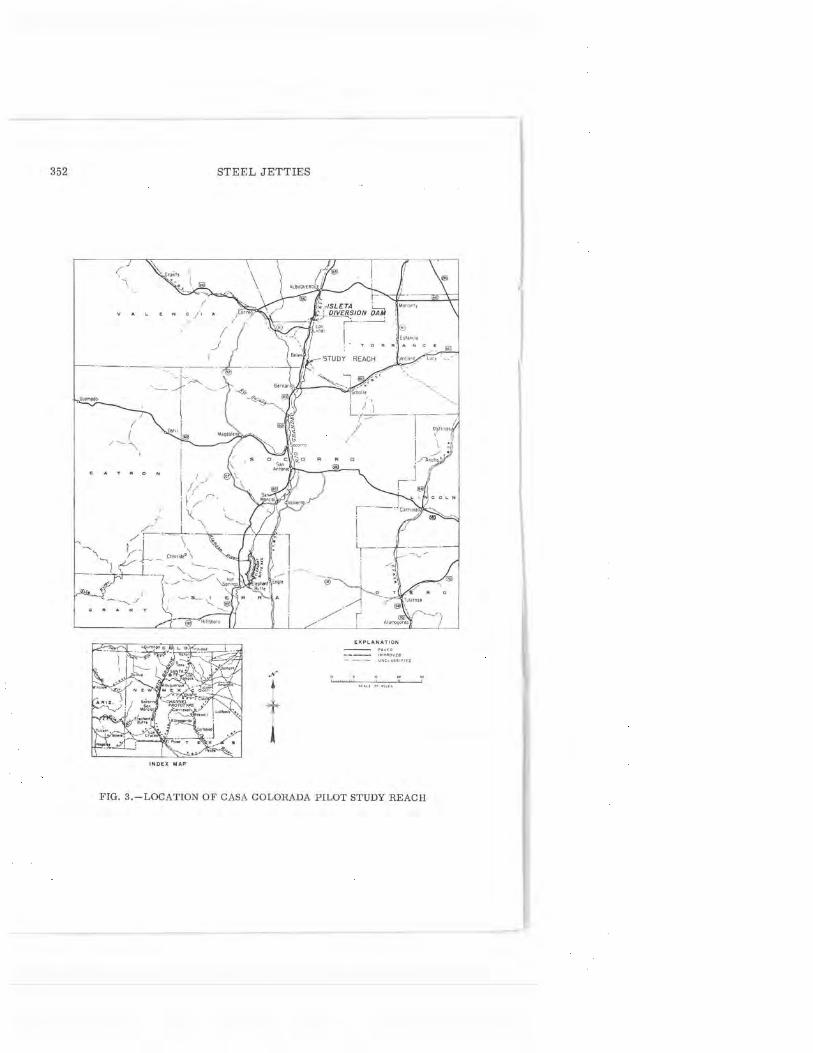
In preparation for a general channelization program for the Middle Rio Grande Project, a 2-mile river reach near Belen, N. Mex. (Fig. 3), was selected for a pilot study. Jetty fields were designed for the prototype pilot reach and were installed both in the field and in a hydraulic laboratory model.

In designing the jetty fields for the Casa Colorada pilot reach, a study was made by USBR hydrologists to determine a design discharge and design channel width. Difficulties were encountered because of the peculiar character­istics of the Rio Grande River. These included days of zero discharge, large fluctuations in discharge during a particular runoff, and two distinct runoff seasons, each with its own characteristic sediment load. Using several meth­ods of determining dominant or design discharge resulted in values ranging from 900 cfs to 13,000 cfs. A value of 5,000 cfs was selected for design. This is the lowest discharge that is difficult to handle. Larger discharges would probably occur, but these would not present as great a problem.

Several methods of computing the design channel width were used, result­ing in values ranging from 330 ft to 770 ft. A value of 600 ft was selected for the design channel width.

Movabl e -Bed Model of Pilot Reach. -The pilot river model was constructed with a horizontal scale of 1 to 140 and a vertical scale of 1 to 22, which gives a distortion of 1 to 6.36. The model represented the area in the prototype between the levees and between ranges 118.15 andl16.26. A plan of the model is shown in Fig. 4.

In order to duplicate the jacks and jetty field in the movable-bed model, 1/ 2-in. mesh galvanized screen (hardware cloth) was used. The screen was bent in a zigzag shape to give the same head loss as a line of jacks. The bent wire mesh was first tested in a fixed-bed, 1 to 16 scale model to determine the density of screen required to duplicate the velocity reduction from a line of jacks. Thewiremeshrequiredforthemovable-bed model was then designed

7 "Hydraulic Model and Prototype Studie s of Ca sa , Colorado Channelization-Middle Rio Grande Project, New Mexico," Report HYD-477, Hydr. Lab., Bur. of Reclam. , U. S. Dept. of the Inte rior, Denver, Colo., May , 1961.

352

Ouemado

(

".

INDEX MAP-

STEEL JETTIES

.I'

t EXPLANAT IO N

---- I M PROVED

~·-···- UNCL~S 5 I F1E0

FIG. 3 .-LOCATION OF CASA COLORADA PILOT STUDY REACH

" ,, I' I \

\

' \ \

>-------, ----Drivin g Pump line

: \ ' \ I '

I \\

f ~ Wire mesh cut

MODEL SCALE 1:140 HORIZONTAL

1:22 VERTICAL

' ' ' ' ' ' \ ' '' '' ,,,

,, ' , , Water inlet------, ~ - - - - - - - - -- -- - - - - - - - - - - - - - - - - - - - - - - - - - - - - - - - -- - - - - - 70 ' ± - - - - - - - - - - - - - - - - - - - - - - - - - - - - - - - - - - - - - - - - - - - - - ->-:

0 10

SCALE OF FEET

FIG. 4. - LAYOUT OF CASA COLORADA RIVER REACH, MOVABLE-BED MODEL

354 STEEL JETTIES

to have a similar projected area per unitlength for the distorted scale. Fig. 5 shows the three methods of representing lines of jacks in the fixed-bed and movable-bed model studies.

The model was operated to simulate an averaged hydrograph in steps of 5,000 cfs with a maximum discharge of 15,000 cfs, and a minimum discharge of 5,000 cfs. The total volume of water discharged during the hydrograph peri­od in the model simulated the total volume of water discharged in the proto­type in a similar period.

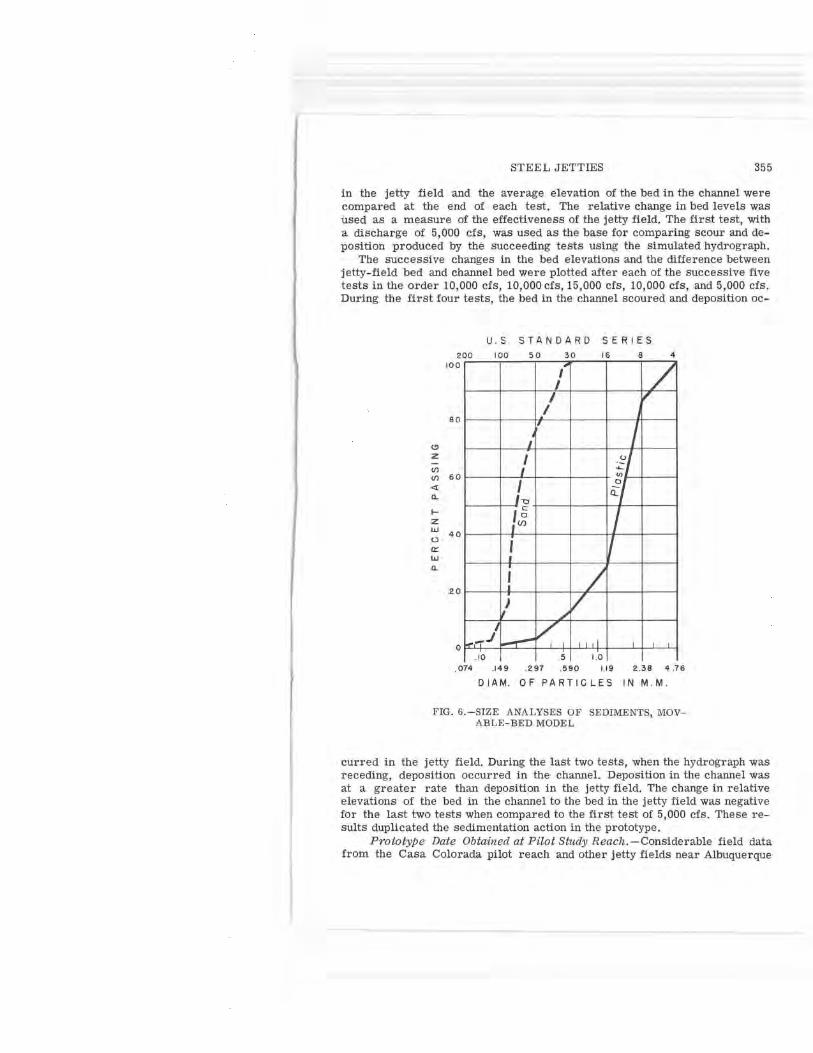
Two model sediments were used to represent the prototype material. A white uniform sand with mean diameter of 0.2 mm represented the bed load,

(a) Lines of 1: 16 Scale Jacks (b) Lines of Jacks Represented by 1/211

Wire Mesh, for 1: 16 Scale Model

(c) Lines of Jacks Represented by 1/2 11 Wire Mesh, for Movable Bed Model, Scale 1:140 Horizontal, 1 :22 Vertical

FIG. 5.-TiffiEE METHODS OF REPRESENTING LINES OF JACKS IN MODEL STUDIES

and a lightweight plastic represented the suspended load. The black color of the plastic material made it easy to distinguish between suspended and bed-load deposits. The size analyses of these two sediments are shown in Fig. 6. The settling-velocity characteristics of the plastic material are shown in Fig. 7. The control weir at the downstream end of the model was shaped to represent the natural river cross section.

Six tests were made, and at the end of each test, cross-section elevations of the movable bed were measured at six ranges in the model. In order to determine the effectiveness of the jetty fields, the average elevation of the bed

STEEL JETTIES 355

in the jetty field and the average elevation of the bed in the channel were compared at the end of each test. The relative change in bed levels was used as a measure of the effectiveness of the jetty field. The first test, with a discharge of 5,000 cfs, was used as the base for comparing scour and de­position produced by the succeeding tests using the simulated hydrograph.

The successive changes in the bed elevations and the difference between jetty-field bed and channel bed were plotted after each of the successive five tests in the order 10,000 cfs, 10,000 cfs, 15,000 cfs, 10,000 cfs, and 5,000 cfs. During the first four tests, the bed in the channel scoured and deposition oc-

<!)

z CJ)

CJ)

<t c..

t--z LL.I

0 er LL.I c..

200 100

80

60

40

20

U.S . STANDARD SERIES

100 50 30 16 8 4 ,

/ I I

I II' / j

I

I j

I

I ti I

I q h, I [5 I U) I .

I I I .

/ I I .

/ J I ,/

' .... -J 0

. 074 ----V

I I I I ,I I I I

.10 .5 1.0 .149 .297 .590 1.19 2 .. 38 4 .76

DIAM. OF PARTICLES IN M.M.

FIG., 6.-SIZE ANALYSES OF SEDIMENTS, MOV­ABLE-BED MODEL

curred in the jetty field. During the last two tests, when the hydrograph was receding, deposition occurred in the channel. Deposition in the channel was at a greater rate than deposition in the jetty field. The change in relative elevations of the bed in the channel to the bed in the jetty field was negative for the last two tests when compared to the first test of 5,000 cfs. These re­sults duplicated the sedimentation action in the prototype.

Prototype Date Obtained at Pilot Study Reach.-Considerable field data from the Casa Colorada pilot reach and other jetty fields near Albuquerque

356 STEEL JETTIES

10

8 ~

Water at 23°G ~

6 Specific gravity= I. 056 /

/ i/

4 <fl a: w 3 I-w ::;;

....J

....J 2

::;;

z

w ....J (.)

I- 1.0

a: <[ . 8 c..

- ~

/ 7

_/

/ V

/ V

/ u. 0 .6

a: w I-

/ /

V w ::;; .4 <[

Cl

,I

/ I

.3

J

I .2

0. I I

0 I 2 3

SETTLING VELOCITY CM./SEC.

FIG. 7.-SETTLING-VE LOCITY CHARACTERISTICS OF PLASTIC MATERIAL, MOVABLE-BED MODEL

.... w w u.

I

I

10 0

I of I

0

I )

0/

of .... 5 a_

w 0

' 0

I 0 ....

<t,\.. ()

0 C 0 0

0 ,1>

0 .01 .02 .03 .04 .0 5 .06 .07 .OB .09 . 10 .II

MANNING'S "n" VALUE

FIG. 8.-MANNING'S n-VALUE VERSUS DEPTH, PROTOTYPE DATA

10

9

0 z 0 0 w u,

.... w w u.

>- 4 ':: <..)

0 ..J w >

0

of 0

L 006

J/~ ro 0 lo :l

\ 0

\ ~)

......

.01 .02

0 ----0 0

.03 .04 .05 .06 .07

M A N N I N G's "n" VA Lu E

0

.08 .0 9 .1 0

FIG. 9.-MANNING'S n-VALUE VERSUS VELOCITY, PROTO­TYPE DATA

358 STEEL JETTIES

were furnished by the Middle Rio Grande Project. Data were obtained at range lines corresponding to measuring stations on the laboratory pilot model. Most of the data were obtained during the months of April through June, which is the runoff season with the lowest sediment load. The field data consisted of river cross sections, discharge measurements, suspended sediment load and size analyses, bed material size analyses, and slope measurements.

Before a generalized study of tieback spacing was conducted, a thorough analysis of the prototype data was made, the purpose being to obtain knowledge

10

9

0

\ '

8

7

\ 0

~

' I- 6 0 LL.I 0 LL.I LL

5 J: I-a.. LL.I 4 Cl

3

0 /'

0 o/ , 2

0 ~ 0 ~

~o

01t5' ~g i----

0 2 3 4 5 6 7 8 9 10

VELOCITY (FEET I SECOND)

FIG. 10.-DEPTH VERSUS VELOCITY, PROTOTYPE DATA

of the action of the river, to verify the model, and to modify the theoretical scale ratios when inexact scaling was detected.

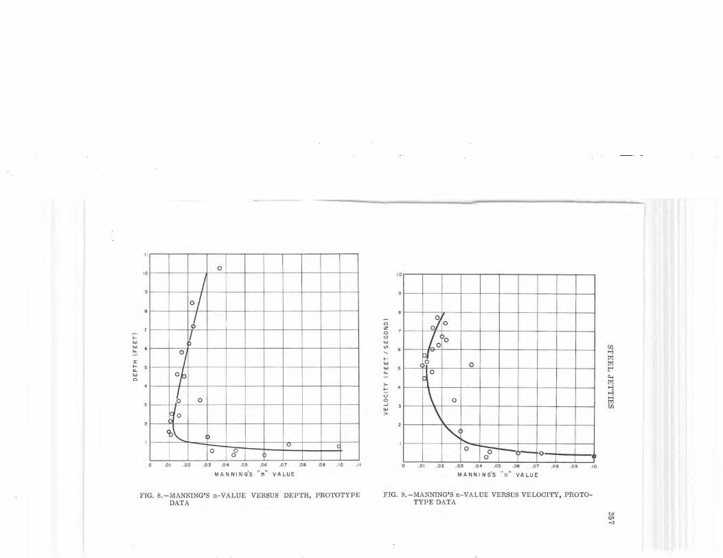
Manning's n-values were computed assuming that the slope associated with each point was equivalent to the average slope across the measuring section. A plot of point depth versus point n-value was made. Another plot of point velocity versus point n-value was made and a third plot was made of point depth versus point velocity. Three curves were first fitted to the data by eye, then adjusted to be consistent with each other, considering equal by the depth

STEEL JETTIES 359

28

0

I I O b

I

27

26 7 7

25

24 J 0

Note: Solid points repre se nt double data points.

23 C

22

21

I

7 -20

01

19 I 'I 0

18 to

' N

It 17 I ...

16 0

"' 0 15 UJ

a: 0 z 14

J 0

V 0 0

/ 0 0

::, :c

~ 13 ~ .I " UJ 12 a:

" II

10

0

/ u

0 I/ k, 0

0 0 Vo 9

8

J. 0

0

7 0

0 0

0 'djo " 0

- 0

7

0 7 1

j

I/ ~

/ / I

0 10 12 13 14 15 16 17 18 19

RIVER WIDTH IN HUNDREDS OF FEET

FIG. 11.-FLOW SECTION AREA VERSUS WIDTH, PROTOTYPE DATA

360

28

27

26

24

23

2 2

2 1

20

,.

18

... O 16

"' ~ 15 0: 0 Z 14 ::, :,:

z 13

<I W 12 0: <I

I I

10

4

~

/ I .. v

/"

STEEL JETTIES

T

Note ; Soli d poi nts represent doub le dot e poi nts.

0

0

0

0 0

0

0

fOlf ... ,_

... -~ -- CURVE COMPUTED FROM FIG. II. ' ' '-' 0

0

0

u

0 \

0

u

0

I J

V

0

0 0

0

0

"' ..:._

"' 7a . 0-,,-OJ 0 ,

[7 0

2

DEPTH - FEET

0

u

0

0

'

FIG. 12.-FLOW SEC TION AR EA VERSUS DEPTH, PROTOTYPE DAT A

-0

,u

-

STEEL JETTIES 361

and velocity measurements. The adjusted curves are shown in Figs. 8, 9, and 10. The original curves were fitted to 150 data sets taken from points that were not near sudden changes in bed profile or a line of jacks. All sets of data were in the design channel. Twenty-one sets of these data, selected in a random manner by rolling a die, were replotted to show the range of data and its scatter. These points are the circles in Figs. 8, 9, and 10.

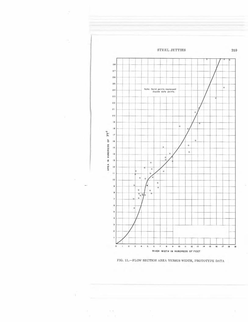
A plot of the average width versus the average area computed from dis­charge measurements was made . A gap was found in the field data for areas smaller than 500 sq ft, and it was necessary to approximate the lower part of the curve. Consequently, an average cross section was determined using the

' I

' I ' I -1-- '-

,_,_ I

I/ ' . ' --! '-- I .

~

' - 17~ ' / I/

f-- - - - t--1------~

' / ,-v /

L/ :p:

" o 02 0;4 O.i OIi lO 1,2

OEPTH · FEET I I 2.0 O 2 3 4 ~ i; 7 O fl Dt. ,03 .0- .D!! t.w; fJ1 0 7 4 , 8 (I ll 14 16 18

VELOCITY FEET PER SECOND MANNING'S ""' VALU! WIDTH • HU'-'OREOS FEET

. '

~ I '

' ' . ' . '

' ' ' "

1--~-

/

-

17 /

/ V

v /

I 10 12 1• ~ ie 20 t2 24 21i

AREA - HUNDREDS OF FEET!

_ lL /

-

-~

FIG. 13 .-RIVER CHARACTERISTICS, P ROTOTYPE DATA

lowest discharge measurement at three stations and widths and areas for lower water surfaces were obtained assuming that the cross section did not change its shape for lower discharges. Thecurvein Fig. 11 for areas smaller than 500 sq ft is the result of these calculations. The average depth of flow versus area curve, Fig. 12, was obtained by dividing flow areas from the curve in Fig. 11 by corresponding widths, in order to obtain depths.

Using the point-data curves and the area curves, the average river char­acteristics were computed and are shown in Fig. 13, plotted against total dis­charge. The curves of Fig. 11 through 13 show that the maximum scatter

362

E .10

E r- .16

z UJ :,; 0 .14

UJ V,

.12 0

0

Z .10 UJ a. V,

::, .08 V,

u_

0 .06

UJ N

ui a: UJ z

.04

U: .02

~ 0 O>

/ V

/v V

STEEL JETTIES

_.,,,.

./" /

./ V

./ V

./"' //

VELOCITY - FEET/ SECOND IN JETTY FIELD OR DESIGN CHANNEL

FIG. 14.-90% FINER SIZE OF SUSPENDED SEDIMENT VERSUS VELOCITY OF JETTY FIELD OR DESIGN CHANNEL

0 z 0

" w ,n

QC •

w 0.

>­w w u_

>- 3 >-

" ~ w >

' /

/ I//

J

/ V

./ V

/ /v

/ /

/ V

V I

I I

I

10 12

CONCENTRATION IN THOUSANDS OF P.P. M.

FIG. 15.-VELOCITY VERSUS CONCENTRATION, PROTOTYPE DATA

STEEL JETTIES 363

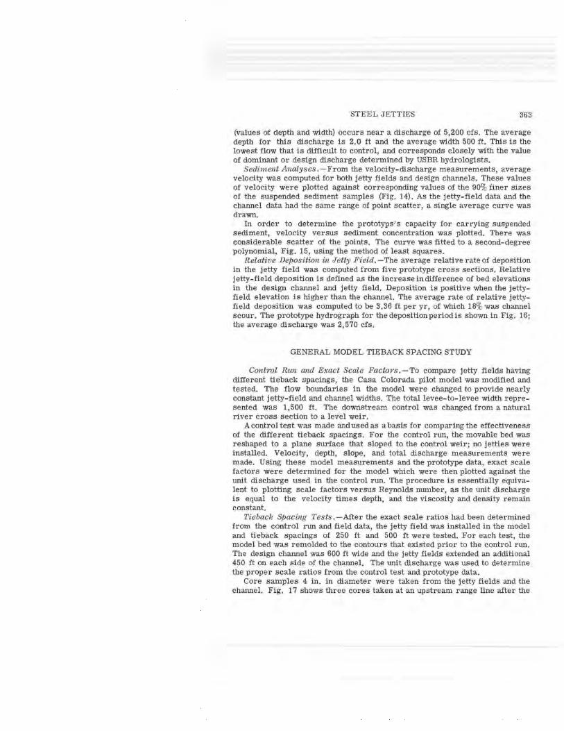
(values of depth and width) occurs near a discharge of 5,200 cfs. The average depth for this discharge is 2.0 ft and the average width 500 ft. This is the lowest flow that is difficult to control, and corresponds closely with the value of dominant or design discharge determined by USBR hydrologists.

Sediment Analyses. -From the velocity-discharge measurements, average velocity was computed for both jetty fields and design channels. These values of velocity were plotted against corresponding values of the 90% finer sizes of the suspended sediment samples (Fig. 14). As the jetty-field data and the channel data had the same range of point scatter, a single average curve was drawn.

In order to determine the prototyps' s capacity for carrying suspended sediment, velocity versus sediment concentration was plotted. There was considerable scatter of the points. The curve was fitted to a second-degree polynomial, Fig. 15, using the method of least squares.

Relative Deposition in Jetty Field. -The average relative rate of deposition in the jetty field was computed from five prototype cross sections. Relative jetty-field deposition is defined as the increase indifference of bed elevations in the design channel and jetty field. Deposition is positive when the jetty­field elevation is higher than the channel. The average rate of relative jetty­field deposition was computed to be 3.36 ft per yr, of which 18% was channel scour. The prototype hydrograph for thedepositionperiodis shown in Fig. 16; the average discharge was 2,570 cfs.

GENERAL MODEL TIEBACK SPACING STUDY

Control Run and Exact Scale Factors. -To compare jetty fields having different tieback spacings, the Casa Colorada pilot model was modified and tested. The flow boundaries in the model were changed to provide nearly constant jetty-field and channel widths. The total levee-to-levee width repre­sented was 1,500 ft. The downstream control was changed from a natural river cross section to a level weir.

A control test was made and used as a basis for comparing the effectiveness of the different tieback spacings. For the control run, the movable bed was reshaped to a plane surface that sloped to the control weir; no jetties were installed. Velocity, depth, slope, and total discharge measurements were made. Using these model measurements and the prototype data, exact scale factors were determined for the model which were then plotted against the unit discharge used in the control run. The procedure is essentially equiva­lent to plotting scale factors versus Reynolds number, as the unit discharge is equal to the velocity times depth, and the viscosity and density remain constant.

Tieback Spacing Tests. -After the exact scale ratios had been determined from the control run and field data, the jetty field was installed in the model and tieback spacings of 250 ft and 500 ft were tested. For each test, the model bed was remolded to the contours that existed prior to the control run. The design channel was 600 ft wide and the jetty fields extended an additional 450 ft on each side of the channel. The unit discharge was used to determine the proper scale ratios from the control test and prototype data.

Core samples 4 in. in diameter were taken from the jetty fields and the channel. Fig. 17 shows three cores taken at an upstream range line after the

364 STEEL JETTIES

6000 I I

~~

l I '/

DAILY DISCHARGE __ /,J I.,./

5000

IJ\ ~

~ /~ - " AVERA( E FOR TIME r-• lv \<\ """ SHOWN 2570 C.F.S. -L' V

\ A. •, \

~~ J J '\

\ /' '

4000 in u: 0 w <:>

3000 a: 4 :i:: <.) en Q

2000

11 1000

AVG. FOR MONTH-, ,J ,-,q "-/' I---\ ... -·~i--0

MAR. APR . MAY JUN. JUL. AUG.

FIG. 16.-1957 HYDROGRAPH OF RIO GRANDE NEAR BERNARDO, N. MEX .

• . • •• c I

FIG. 17.-CORE SAMPLES OF BED TAKEN FROM RIGHT JETTY FIELD, DESIGN CHANNEL, AND LEFT JETTY FIELD IN UPSTREAM CURVE

STEEL JETTIES 365

test conducted with 250-ft tieback spacing. The core showing the greatest depth of black plastic sediment was on the inside of the curve. Deposits in the jetty field on the inside of the curve tended to crowd the flow into the chan­nel and into the jetty field on the outside of the curve. The results of these tests indicated that jetty-field installations should be constructed only on the outside of curves, initially, and should be constructed on the inside of curves only when the need develops.

FRICTION FACTOR ANALYSIS

A friction factor analysis was made of the tieback spacing data obtained in the model tests. Because the friction factor expressed by the Darcy­Weisbach equation is dimensionless, it was used to provide data for both model and prototype uses. For open-channel flow, assuming that the hy­draulic radius is equal to depth, the friction factor may be expressed as

f = 8 g (7) .................. (5)

in which Sis the slope. By substitution in Eq. 5, friction factors were computed and related to

unit discharge with the relative tieback spacing x/ y used as a parameter (Fig. 18). Fig. 18 shows that the values of f become constant for discharges greater than approximately 10 cfs per ft of width corresponding to values of Reynolds numbers near 1 x 106 and greater. These curves are typical of friction head loss. For convenience of design computations described in Ap­pendix I, the same data are presented in terms of percentage increase of friction in Fig. 19.

PREDICTING JETTY-FIELD DEPOSITION

Using field data from a proposed jetty-field site and the friction factor analysis of this study, predictions can be made of the rate of jetty-field de­position. Details of sample computation are given in Appendix I. In this com­putation for a 2-mile long jetty field on each side of a 500-ft design channel, the tieback spacing is 250 ft and the levee-to-levee river width is 1,400 ft. Using the pre-installation river characteristics similar to those in the Casa Colorada reach, the computed average rate of relative jetty-field deposition was found to be 2.16 ft per yr.

CONCLUSIONS

Both model and prototype studies indicated that jetty fields are successful in alining rivers that carry appreciable quantities of suspended sediments. In order to compute the relative rate of sediment deposition, field data are required. The use of point-data analysis, described herein, aids greatly in extending field data and establishing river-characteristic curves.

"' > .....

0.05

>- 0.04

<1) CJI

ID

II

... a:: 0.03

~ 0

~ z 0

t; 0.02

a:: LL

\ JACKS MADE LACED WITH

\ ' \ ', , ......

\ ',, ... ------I'-. - ---,, -----. '

~ ..... _ -- .. ............ ... . ... ............ -

...............

3 4

FROM 16 FT. STEEL ANGLES NO. 6. GALV. WIRE

-.... -- ---· ----- ---- --------· ----

·------~-----r--r--. -----.. r--------..-,,p

5 6 7 UNIT DISCHARGE (cfs/ft)

-

- --- ------------ ----- --

- ... ,_ .... -

- ·- . .. ------- --

8 9 10

FIG. 18.-FRICTION FACTOR IN TERMS OF RELATIVE TIEBACK SPACING AND UNIT DISCHARGE

(!)

z 100 0

'If. <1)

~ 125 0 en <X

ID '"1 IJJ t:i:J i= t:i:J

150 ~ IJJ "-< > t:i:J i= '"1

200 '.5 '"1 -IJJ t:i:J n:: en 500

00

140

z 0 120 .:: ~ a: i..

:!:

~ 100 <( LL1 a: 0 :!: LL1 <!)

~ 80 z LL1 0 a: LL1 Cl.

~ 60

40

20

STEEL JETTIES

I

I

ff I (J

~ V JACKS MADE FROM ~ ~ <r

16 FT. STEEL ANGLES o/ I LACED WITH NO. 6 WIRE ./:! CJ

;;; ' I/ / ! ~I I ~I

~o/ I J V

t; ( /

_,,,.-

I V1 ~ V ~/

JI I l/1 / /1 Vj V i----o.__...

~ ~ V V .,..

~ ~ V V '3 / ---

~ V .... V --- __..,.,... - --

.002 .004 .006 .008 .010

RECIPROCAL OF RELATIVE TIEBACK SPACING

FIG. 19.-PERCENTAGE INCREASE IN FRICTION FACTOR IN TERMS OF RELATIVE TIEBACK SPACING AND UNIT DISCHARGE

367

TABLE !.-COMPUTATION OF AVERAGE RATE OF RELATIVE JETTY FIELD DEPOSITION FOR HYDROGRAPH YEAR

Discharge, Q, Average relative Method of Average deposition Percentage of

deposition, obtaining relative for time interval, time, from in cfs in ft per yr deposition in ft per yr flow-duration curve

(1) (2) (3) (4) (5)

0 0 0.00 2,60

10 0 0.00 83.40

2,000 0 Extrapolated 1.68 3.20

2,570 3.36 Field Data 9.68 5.20

5,000 16.0 Interpolated 21 .40 2,50

7,500 26.8 Computed 32 .00 2.15

10,800 37.2 Computeda 41.40 0.60

15,000 45.6 Extrapolated 47.00 0.18

17,000 48.4 Extrapolated 49.90 0.10

20,000 51.4 Extrapolated -- 0.07 ---100,00

asee sample computations in Table 3. Average rate of deposition = 216.31/100 = 2.16 ft per yr

Weighted average, deposition x 100,

Col. 4 x Col. 5 (6)

0.00

o.oo

5.38

50.34

53.50

68.80

28.84

8.46

4.99

-----216.31

STEEL JETTIES 369

To determine the design discharge, it is recommended that width and depth be plotted versus flow area and that a value be selected that corresponds to the flow area having the maximum scatter or deviation of data points with respect to depth and width. This is the lowest discharge that will be difficult to control. The average river width corresponding to this discharge should be used for the design channel width.

The relative rate of deposition in a jetty-fieldinstallation can be computed by the procedure demonstrated herein. However, future studies may indicate desirable modifications and refinements in the procedures.

APPENDIX !.-COMPUTING DEPOSITION IN A JETTY FIELD

Jetty-field installations can be designed using field data and the friction factor analysis presented previously. To illustrate the method of predicting

TABLE 2.-COMPUTATION FOR ONE DESIGN CHANNEL UNIT DISCHARGE IN FIG, 21

Design Jetty Channel Field

~ 0 .

.s "' ...., ~

~ ...; ...., 0 Q) C,) "d II o A

&t ~ gJ >,.~ Q) § "d.::: 0

"' 0.

.~ ..d' ~..o rz. gJ II S § Q).,... o rn "' "d s . "d ~ 0. ..8 .& i,; CX)

0 "d s 0 .o ... 0 Q) :.a..-1 ~ Q)

~ .s b~ C! .s ~ 0 AO'~ o· ..o s 8 §~

... "d oj oj '-- 0 fill~~ ~~ .,.C\l ,.. o~

A "d "d • :,: Q)~ ... 43 CJ + S:::$ ;;l~ :§ ~ ~~ ""' >, II ..... ,o oj O • .::: rn...; s 0

,,-< '-- g [/) [/) >, LC",) 11 .::: gJ .:::.:::'--0 .9 "a~ •,-< '-- ..... :~ :g ~f "' ooJSoo

::dl ~~ .e,.s II ~ :8 g :;j~ CJ I"""'! b cd • >< rn ~ II ·.-1 II <D ... 0 ..0 .9 -0 ~ b!l rn c3 :S .s t~ Q) ..... t:.!!;'1 ~Jx Cl)•.-1 Q) -~~o' < O' >-, >, >-, > P-+ ~ •.-I t:ll<O~ ~ :0 0~ ..... ...., (1) (2) (3) (4) (5) (6) (7) (8) (9)

10 6,44 1.00 6,44 0.00 52 0,004 29 0,017 0.0219 10 6.44 1.50 4,29 0,0174 0,006 53 0,017 0,0260 10 6.44 2 ,00 3,22 0,0411 0,008 91 0,017 0,0325 10 6.44 2 ,50 2,58 0,0802 0,010 121 0,017 0,0376

Note.-Tieback spacing, x, 250 ft; channel width, 500 ft; levee-to-levee width, 1,400 ft; total river discharge, 10,800 cfs. Depth in jetty field for qc = 10 cfs/ft is 1,86 ft, which is determined by interpolating or by cross-plotting Cols, 5 and 9 with respect to Col, 3.

the changes in the river bed when a jetty field is installed, a sample problem pertaining to channelizing a reach of the Middle Rio Grande is explained.

Tables 1, 2, and 3 show the step-by-step procedures for making the cal­culations and tabulating the results in convenient form.

The basic data needed to predict the scour and deposition in the bed of a jetty-field installation are similar to the prototype data analyzed previously.

370 STEEL JETTIES

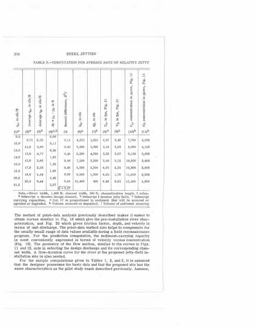
TABLE 3,-COMPUTATION FOR AVERAGE RATE OF RELATIVE JETTY

<J':) <J':) ..... ..... bn bn i£: i£: ~- ~-s s

>, 8: p.

~ "' p. ¢: '<:I .s .s ....._

..f!l ..f!l ¢: ai ..... ..... A "' "' A

" " " .s .s .s A bn bn .s .s <D ti ti H i£: i£: ¢: J t: <D H H ffe ..... 1'l .., ....._

'.!:I oo· 00 A ..f!l I ..f!l ..f!l <D <D

fil, fil, "Cl -9< -9< § " " ~ 'tl " " A .s el el A .s .s .s .s 0

H H II 0 " " J

<D <D " C) cl 0 .::. Cl .::. > ~ >, <D

~ "<:] 00 G' :> :> u u

(l)a (2)a (3)b (4)a,b (5) (6)a (7)b (8)a (9)b (lO)b (ll)b

9,5 0,00 9,75 6,58 0,11 4,875 5,925 4,97 3,40 7,700 4,350

10,0 0,11 11.0 5,88 0.45 5,500 5,300 5,16 3,29 8,200 4,150

12.0 0,56 13,0 4,77 0,46 6,500 4,300 5,50 3,07 9,150 3,850

14,0 1.02 15,0 3,66 0.48 7,500 3,300 5,80 2,75 10,050 3,400

16,0 1.50 17,0 2,55 0,46 8,500 2,300 6,05 2.35 10,900 2,950

18.0 1.96 19,0 1.44 0.50 9,500 1,300 6.25 1.70 11,650 2,300

20.0 2,46 20,8 0.44 0,81 10,400 400 6.46 0.65 12,400 1,000

21.6 3.27 ~ = 3,27

Note.-River width, 1,400 ft; channel width, 500 ft; channelization length, 2 miles; a Subscript c denotes design channel. b Subscript f denotes jetty field. c Subscript

carrying capacities. e Col. 17 is proportional to sediment that will be scoured or agraded or degraded. h Volume scoured or deposited. i Volume of sediment scouring

The method of point-data analysis previously described makes it easier to obtain curves similar to Fig. 13 which give the pre-installation river char­acteristics, and Fig. 20 which gives friction factor, depth, and velocity in terms of unit discharge. The point-data method also helps to compensate for the usually small range of data values available during a field reconnaissance program. For the prediction computation, the sediment-carrying capacity is most conveniently expressed in terms of velocity versus concentration (Fig. 15). The geometry of the flow section, similar to the curves in Figs. 11 and 12, aids in selecting the design discharge and its corresponding chan­nel width. A flow-duration curve for the river at the proposed jetty-field in­stallation site is also needed.

For the sample computations given in Tables 1, 2, and 3, it is assumed that the designer possesses the basic data and. that the proposed site has the same characteristics as the pilot study reach described previously. Assume,

STEEL JETTIES 371

FIELD DEPOSITION FOR TOTAL RIVER DISCHARGE OF 1 8, 000 CFS

C!) - I C!) .... C!) 0 I .... I .... 0

0 X .... "' 0 ....

X .... u X ~-0 I ~- ;::J .gJ

C!) C!) C)

C: I C!) u I I.O O' .s 0 0 I 0

.... ti) S!l C) .... 0 + .... ] .s C) Ql ..-< 0 Q) ti)

X X "' X H s .s ..-< Cl! £ ro· .s C) ..... H s ;::J 00 u u 0 u "! Ql 0 ...;-C) ..... H &l H ti)

(§ (§ u (§ .... < :> :> <:]

(12)a,d (1 3)b,d (14)d (1 5)a,d (16) (l 7)e,f (1 8)g (19)h (20)i (2l)i

37.5 25 .8 63.3 74 Depos it 12.8 9.5 1.04 8.87 0 .12

45.1 22 .0 67.1 74 Depos it 8.28 9 .5 4.2 8 5.74 0.75

59. 5 16.6 76.1 74 Scour - 2.52 5.28 2 .38 1. 74 1.37

75 .4 11.2 86.6 74 Scour -15.1 5.28 2.53 10.5 0.24

92.6 6.78 99.4 74 Scour -30.5 5.28 2.43 21.1 0.12

111.0 2 .99 114.0 74 Scour - 48.0 5.28 2.64 33.3 0.0 8

129.0 0.40 129.0 74 Scour - 66 .0 5.28 4.28 45. 7 0 .09

r~ 2.11

tieback spacing, 250 ft . r denotes unchannelized river . d Q x C t e rms are proportional to suspended-sediment deposited. f The factor 1-2 converts suspended load to total load. g Area that is or settling per second. i Time used in obt a ining Col. 19.

then, that the designer desires to investigate a proposed installation with a length of 2 miles, a levee-to-levee width of 1,400 ft, and a tieback spacing of 250 ft.

First select a design discharge and corresponding design channel width. The deviations in width and depth in Figs. 11 and 12 show that the design width should be approximately 500 ft. The corresponding river discharge of approximately 5,000 cfs is determined from Fig. 13. This width corresponds to the lowest discharge that is most difficult to control.

For convenience, and to simplify the computations, the process of scour and deposition is assumed to occurnonconcurrently, with deposition occurring only in the jetty field and scour occurring only in the channel. Both deposition and scour are considered as relative deposition. In actual installations, deposition and scour may or may not occur at the same time. The information desired is the average rate of relative deposition in the jetty field for the

w <!)

60

50

! 30 :,: <.)

"'

z 20 :,

10

J V

~i---

L.>, ~-V

.,.,.....-,,.,..- ~

V \ [,A- --DEPTH

k -FRICTION I/ FA CTDR /

I V p--• -VELOCITY

I V I I

I I I I/

I J V

I........_ V" -10 12

DEPTH AND VELOCITY AND lfx IOD) (FEET) (FT/SEC)

FIG. 20. - DEPTH, VELOCITY, AND FRICTION FACTOR VER­SUS UNIT DISCHARGE, PROTOTYPE DATA

22

21 ~

_J

w z

16

Z 17 <t :,: <.)

z 16

w <!) 15 a: <t :,: <.> 14

"' a I- 13

z

12

I

0

9 0

\ r

"' t- ---- CHANNEL DEPTH I " I"--. ..

\ '\ I I I\

\ \ I \ I TOTAL DISCHARGE

~-10,soo cfs

*, I J

\ X I \ II \' --- ---JETTY FIELD j VELOCITY .,~

I I/ \ I 1\ I

JETTY FIELD A I \ CHANNEL -i VELOCITY----DEPTH--

\ I \ I ' \ 'i

DEP T H AND VELOCITY (FEET) (FT/SEC)

FIG. 21. - CHANNEL AND JETTY- FIELD PROPERTIES DETER­MINED FROM MODEL AND PROTOTYPE DATA

STEEL JETTIES 373

selected tieback spacing, and the time for the river to become completely channelized.

Table 1 is a computation table for determining the average relative de­position for the jetty-field reach for a typical year. This is accomplished by determining the average relative deposition (Col. 2) for steps in discharge as related to a flow duration curve for the river. In the example, prototype data were available to determine the average rate of deposition for a dis­charge of 2,570 cfs. The yearly rate of deposition amounted to 3.36 ft per yr, assuming that the discharge of 2,570 cfs was constant throughout the year. For other values of constant river discharge shown in Col. 1, the average relative deposition, Col. 2, can be computed by the method explained subsequently and in Tables 2 and 3. For the example examined herein, average relative deposition was computed for 7,500 cfs and 10,800 cfs. For the other values of discharge, deposition rates were extrapolated or inter­polated from a plotted curve, Col. 3. The average rates of deposition for the intervals between discharges are listed in Col. 4. The corresponding per­centage of time on the flow-duration curve for the discharge interval is entered in Col. 5. The flow-duration curve for the Rio Grande gaging station near Bernardo, N. Mex., as compiled for the years 1936 through 1954 was used in this example. The weighted average deposition for each discharge interval, Col. 6, is obtained by multiplying the values in Col. 4 by the values in Col. 5. A summation of Col. 6 divided by 100 gives the average rate of relative deposition (deposition in the jetty field or scour in the channel or both) for a typical year. The rate for this example is 2.16 ft per yr.

The method for computing the average rates of relative deposition, Col. 2, for the discharge steps in Col. 1 will now be described. This is the basic process for computing deposition in a jetty field. The computations are shown in Tables 2 and 3. For the remainder of the example, only the computations for the constant river discharge of 10,800 cfs will be explained.

Table 2 shows a sample computation for determining the resulting depth in the jetty field for an assumed unit discharge in the design channel. The ex­ample is for 10 cfs per ft in the channel; the resulting depth is plotted in Fig. 20. Because the channel is 500 ft wide, 5,000 cfs is flowing in the channel, leaving 5,800 cfs in the jetty fields. This quantity, expressed in terms of unit discharge, is 6.44 cfs for two jetty fields each 450 ft wide ( Col. 1 and 2).

Various depths of flow are assumed for the jetty field (Col. 3). From these depths, velocities are computed, (Col. 4). The friction factor corresponding to hydraulic characteristics given in Col. 1 through 4 and using an average slope of 0.000829 is computed and entered in Col. 5. Ratios of assumed depths to the tieback spacing are computed and are listed in Col. 6. The percentage increase in friction factor caused by the tiebacks at the assumed depths is determined from Fig. 19 and appears in Col. 7. The friction factor that would occur at a unit discharge of 6.44 cfs with respect to the bed roughness alone, without a jetty field, is 0.017. This value can be read from Fig. 18 or Fig. 20, and when multiplied by one plus the decimal percentage of friction increase, results in the combined friction for the bed and tiebacks. The depth can be determined by interpolation or by cross plotting Col. 5 and 9 versus Col. 3 on the same coordinates. The jetty-field depth for this example is 1.86 ft. This depth and the corresponding velocity were plotted in Fig. 21 for the unit dis­charge of 10 cfs in the design channel. The values of channel depth and channel velocity for this same unit discharge are determined from Fig. 20. To obtain

374 STEEL JETTIES

curves similar to those shown in Fig. 21, computations must be made for other values of unit discharges in the channel.

The computation of the time rate of relative deposition for the constant river discharge of 10,800 cfs appears in Table 3. Values of unit discharge ( qc) in Col. 1 for the design channel are assumed for the range indicated in Fig, 21. The average channel unit discharge for each interval is entered in Col. 2. By continuity and using the design widths, values of the unit discharge

qf for the jetty field are determined (Col. 3). For each of the assumed values of qc, the differences in depth between the channel and jetty field (ay) are computed from values determined in Fig. 21 and are listed in Col. 4.

From Col. 4, the second differences of depth ( A 2y) for the unit discharge intervals are computed and appear in Col. 5. The values of channel and jetty­field discharges and velocities were determined from the continuity equation, the selected design width, and Fig. 21. The values for these variables appear in Col. 6 through 9, From Fig. 15, the corresponding values of suspended­sediment concentration in parts per million by weight in the channel and jetty field are entered in Col. 10 and 11, respectively. The Q C terms (discharge multiplied by concentration) in Col. 12, 13, and 14 are proportional to the sediment-carrying capacities for the design channel, jetty field, and the entire channelized river reach. The Q C term in Col. 15 is proportional to the river sediment-carrying capacity prior to installation of the jetty field. This term is constant because the computation concerns one total discharge. Whether there is deposit in the jetty field or scour in the channel is noted in Col. 16.

The rate of scour or deposition, whichever occurs, or both, is proportional to the values of the difference between the river sediment-carrying capacity before and after channelization. The sediment-carrying values times a con­stant (1.2) times the unit weight of water divided by the unit weight of the sediment gives the in-place volume of the solids scoured or deposited per second (Col. 20). The factor 1.2 is an approximate value and is used to convert suspended load to total load. In Col. 18 are the areas associated with the scour and deposition. These areas times the change in depth difference, Col. 5, result in the volumes expected to be scoured or deposited at the rate given in Col. 20. These volumes are entered in Col. 19. Dividing the values in Col. 19 by those in Col. 20 gives the incremental times (At) to deposit or scour the incremental volumes (Col. 21). The sum of the values in Col. 21 is the total time for the flow to be completely channelized for the discharge that had originally covered the total jetty-field installation width; this total time is 2. 77 x 106 sec.

The average relative rate of jetty-field deposition is 37 .2 ft per yr for the constant river discharge of 10,800 cfs. This rate was entered in Table 1. In the example, the relative deposition (difference in channel and jetty-field bed elevations) amounted to 3.27 ft in 32 days to reach complete channelization at a constant discharge of 10,8000 cfs.

APPENDIX 11.-NOTATION

b = subscript denoting bed;

STEEL JETTIES 375

C sediment concentration, in parts per million, by weight;

c subscript denoting channel;

F Froude number;

f Darcy=Weisbach friction factor; subscript denoting jetty field; a function;

g acceleration of gravity;

n Manning's friction factor;

o subscript denoting upstream from jetty field;

Q total discharge, in cubic feet per second;

q unit discharge, in cubic feet per secondperfoot of width;

R subscript denoting reduction; relative rate of jetty-field deposition;

r subscript denoting river;

S slope:

t time;

V velocity; volume;

x tieback spacing or distance downstream from a tieback;

y depth of flow;

t:..Y Ye - Yf = difference in depth between channel and jetty field;

t,,.2 y second difference of depth; and

¢ angle between a tieback line and a frontline.

I I

I I

I I

I