hybrid probabilities and error-domain structural ... · goulet, j., michel, c., and smith, i....

Hybrid probabilities and error-domain structuralidentification using ambient vibration monitoring

James-A. Gouleta,∗, Clotaire Michelb, Ian F. C. Smitha

aApplied Computing and Mechanics Laboratory (IMAC)School of Architecture, Civil and Environmental Engineering (ENAC)

ECOLE POLYTECHNIQUE FEDERALE DE LAUSANNE (EPFL)Lausanne, Switzerland

bSwiss Seismological Service (SED)SWISS FEDERAL INSTITUTE OF TECHNOLOGY ZURICH (ETHZ)

Zurich, Switzerland

Abstract

For the assessment of structural behavior, many approaches are available to compare

model predictions with measurements. However, few approaches include uncertain-

ties along with dependencies associated with models and observations. In this paper,

an error-domain structural identification approach is proposed using ambient vibration

monitoring (AVM) as the input. This approach is based on the principle that in science,

data cannot truly validate an hypothesis, it can only be used to falsity it. Error-domain

model falsification generates a space of possible model instances (combination of pa-

rameters), obtains predictions for each of them and then, rejects instances that have

unlikely differences (residuals) between predictions and measurements. Models are

filtered in a two step process. Firstly a comparison of mode shapes based on MAC

criterion ensures that the same modes are compared. Secondly, the frequencies from

each model instance are compared with the measurements. The instances for which

the difference between the predicted and measured value lie outside threshold bounds

are discarded. In order to include ”uncertainty of uncertainty” in the identification

process, a hybrid probability scheme is also presented. The approach is used for the

identification of the Langensand Bridge in Switzerland. It is used to falsify the hy-

pothesis that the bridge was behaving as designed when subjected to ambient vibration

inputs, before opening to the traffic. Such small amplitudes may be affected by low-

level bearing-device friction. This inadvertently increased the apparent stiffness of the

structure by 17%. This observation supports the premiss that ambient vibration surveys

∗Corresponding author: [email protected]

Goulet, J., Michel, C., and Smith, I. (2013). Hybrid probabilities and error-domain structural identification using ambient vibration monitoring. Mechanical Systems and Signal Processing, 37(1–2):199–212.http://dx.doi.org/10.1016/j.ymssp.2012.05.017

Goulet, J., Michel, C., and Smith, I. (2013). Hybrid probabilities and error-domainstructural identification using ambient vibration monitoring. Mechanical Systems and

Signal Processing, 37(1–2):199–212.

should be cross-checked with other information sources, such as numerical models, in

order to avoid misinterpreting the data.

Keywords: Structural identification, Ambient vibration monitoring, Uncertainty,

error-domain identification, Extended uniform distribution, Correlation, Error

1. Introduction

In the early history of dynamic monitoring of bridges, researchers were interested

in the modal properties of these structures. For instance Carder [11], used monitoring

to predict resonance during an earthquake. From the 70s, the development of record-

ing capabilities (e.g. [27]) and of numerical modelling lead researchers to validate

bridge models using experimental ambient vibration data [1]. Later, researchers began

optimizing model parameters to improve the fit between predicted and observed data.

Mottershead and Friswell [32] reviewed some of these applications. Since then, there

has been an increasing popularity for Bayesian-updating methodologies [3, 4]. Many

applications of dynamic monitoring of bridges can be found in the literature, for ex-

ample [3, 9, 13, 14, 23, 26, 31, 33, 38, 40, 41, 46, 49]. Some of these studies, such

as [3] and [14], explicitly included uncertainties in the identification process. These

studies however did not include modelling uncertainties due to aspects such as model

simplification, omissions and mesh refinement.

Error-domain model falsification was proposed by Goulet and Smith [19] for situa-

tions where bias in models introduce dependencies between predictions. This approach

is based on the principle that in science, data cannot convincingly validate an hypoth-

esis, it can only be used to falsity it [36, 45]. Error-domain model falsification is built

upon more than a decade of research [37, 39, 43]. In a previous study [17], a similar

identification approach was used to perform structural identification on bridges based

on static measurements. Error-domain identification was proposed to overcome the

limitations of other approaches based on statistical inference that relies on the correct

evaluation of uncertainties and of their dependencies [5, 44]. Error-domain model fal-

sification generates a space of possible model instances (combination of parameters),

obtains predictions and then falsifies wrong instances based on the difference between

predictions and measurements (observed residual). A model instance is falsified, if the

observed residuals lies outside threshold bounds computed from the combination of

modelling and measurement uncertainties.

2



Elements of error-domain model falsification is presented in Equations 1 to 3. A

model class g(~θ) is used to perform predictions based on vector containing np input

parameters ~θ = [θ1, θ2, θ3, . . . , θnp ]. If real quantities for these parameter are known

~θ∗, the difference between the value predicted by the model and the modelling error

εmodel is equal to the physical quantity R for the system (see Equation 1). The differ-

ence between the measured value y and the measurement error εmeasure is also equal

to this physical quantity. In practical situations, neither errors nor the real physical

quantity is available.

g(~θ∗)− εmodel = R = y − εmeasure (1)

In Equation 2, exact values of errors are replaced by a random variables Umodel and

Umeasure each described by a probability density function (PDF) fU (ε) : R → R+.

The relation used to falsify models can be obtained by reordering the terms in Equation

3. In this Equation, the left-hand term is the observed residual of the difference between

predicted and measured value and the right-hand term is a combined probability den-

sity function fUc representing modelling and measurement uncertainties. Uncertainty

sources are combined using Monte-Carlo methods [15].

g(~θ)− Umodel = y − Umeasure (2)

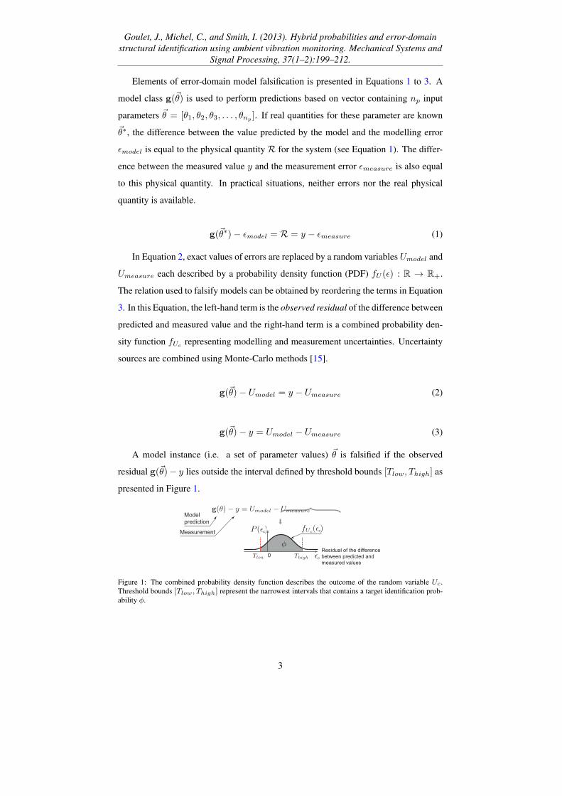
g(~θ)− y = Umodel − Umeasure (3)

A model instance (i.e. a set of parameter values) ~θ is falsified if the observed

residual g(~θ)− y lies outside the interval defined by threshold bounds [Tlow, Thigh] as

presented in Figure 1.

0

}Measurement

Model

prediction

Residual of the difference

between predicted and

measured values

Figure 1: The combined probability density function describes the outcome of the random variable Uc.Threshold bounds [Tlow, Thigh] represent the narrowest intervals that contains a target identification prob-ability φ.

3



When using several measurement locations (comparison point) i ∈ [1, . . . , nm], a

model instance is falsified if the observed residual lies outside threshold bounds at any

location. This condition is presented in Equation 4.

∀i ∈ [1, . . . , nm] : Tlow,i ≤ g(~θ, i)− yi ≤ Thigh,i (4)

Threshold bounds are computed as the shortest intervals that contain a probability

content φ ∈]0 . . . 1]. This can be solved by satisfying the relation presented in Equation

5 for the domain T = [Tlow,1, Thigh,1]×[Tlow,2, Thigh,2]×. . .×[Tlow,nm , Thigh,nm ] ⊆

Rnm .

∀i ∈ [1, . . . , nm] : φ =

∫. . .

∫TfUc,i(εc,1, . . . , εc,nm)dεc,1 . . . dεc,nm (5)

Here, combining modeling and measurement uncertainties allows determination of

the maximal plausible errors (Threshold bounds) for a target reliability φ. Thus, there

is a probability < 1 − φ of wrongly rejecting correct models. Some wrong models

are likely to be kept in the candidate model set if they are close enough to measured

data. This procedure is intended to be conservative because all candidate models are

considered as possible explanations of the behavior. Accepting false models is in most

cases inevitable in order to ensure that the right model will not be wrongly discarded.

As suggested by Beven [6], a model class g(. . .) is falsified when all its model

instances ~θ are falsified by threshold bounds. Falsifying an entire model class is an

indication that there are flaws in the way the system is modeled. No other methodology

in use for structural identification is capable of detecting wrong model classes.

Uncertainty quantification is a task intrinsic to system identification. In addition

to the traditional probabilistic description of uncertainties, other approaches, such as

interval analysis [30] and probability bounds analysis [16, 42], have also been used

to describe imprecise knowledge associated with uncertainties. These alternative ap-

proaches for defining and combining uncertainties are conservative [20]. In the case of

system identification, these approaches can be too conservative, hindering the process

of making sense out of data. When using probability density functions for describing

uncertainties, in many cases, little information is available to accurately quantify them.

The Uniform distribution may not reflect the subjective process of defining uncertainty

bounds. For these situations, the curvilinear and iso-curvilinear distribution [22, 25]

4



have been proposed. When Uniform distributions are used to describe uncertainties,

an uncertainty can also be associated with bound positions. When combined together,

these distributions form the curvilinear distributions as presented in Figure 2. The un-

certainty associated with bound positions is, however, also incomplete.

Error

Pro

ba

bili

ty

Main uncertainty

Uncertainty related to

bound definition

Combined uncertainty

(curvilinear distribution)

Figure 2: Curvilinear distribution that included uncertainty in bound position

In this paper, error-domain model falsification is further developed to allow the use

of ambient vibration monitoring as the input during structural identification. Also, a

new probability distribution is proposed to include the uncertainty involved with the

inexact knowledge of the bounds of uniform distributions. Section 2 describes the

fundamentals behind the use of dynamic input for system identification. This method-

ology is applied to a case study to confirm its applicability for identifying the behavior

of full-scale structures.

2. Error-domain model falsification using ambient vibration monitoring

Experimental modal analysis is not a direct measurement of a physical parameter

(displacement, rotation) but a relatively complex signal processing method allowing

the modal parameters of a structure to be derived, including resonance frequencies,

modal shapes and damping ratios. This analysis is based on the assumption of linear

behaviour. Moreover, Operational Modal Analysis, i.e. under ambient vibrations, as-

sumes that the input motion is of equal amplitude for every frequency (white noise) and

that the recorded data averaged over a sufficient length of time is a direct representation

of structural behaviour (stationary signal).

In this paper, the structural identification process is performed on the resonance fre-

quencies only. However, in order to compare the predicted and measured frequencies, a

correspondence check must be performed between the measured (Φy,j , j ∈ [1, . . . , nj ])

and predicted (Φg(~θ,k), k ∈ [1, . . . , nk]) mode shapes in order to ensure that only the

5



corresponding modes are compared together. When dealing with large finite-element

models, the number of predicted modes nk is, in most situations, much larger than what

is measured nj . Moreover, the order of these modes may be different from one model

instance (~θl) to another. The Modal Assurance Criterion (MAC) [2] (Equation 6, whereH denotes complex conjugate and transpose), is used to perform mode shapes corre-

spondence checks in a first step. When the frequencies corresponding to each mode

shape are found, model falsification is performed based on the observed and predicted

frequencies.

MAC(Φy,j ,Φg(~θl,k)) =

|ΦHy,jΦg(~θl,k)|2

|ΦHy,jΦy,j ||ΦHg(~θl,k)Φg(~θl,k)|

(6)

In order to identify the behavior of a structure, a set containing nl model instances

~θl, l ∈ [1, . . . , nl] is generated to explore the domain of possible solutions. Only sets

{j, k, l} satisfying Equation 7 ∀j ∈ [1, . . . , nj ], k ∈ [1, . . . , nk], l ∈ [1, . . . , nl] are

used to falsify model instances. φMAC ∈ [0, 1] is the modal assurance criterion target

defined by users.

{(j, k, l) ∈ N3 : MAC(Φy,j ,Φg(~θl,k)) ≥ φMAC} (7)

For some model instances ~θ, not all measured (Φy,j) and predicted (Φg(~θ,k)) modes

may pass the MAC correspondence test. Therefore, model falsification may not em-

ploy the same number of modes for all model instances. This approach is conservative

because the confidence interval Ti,Low and Ti,High expressed in Equation 5 are deter-

mined using the full set containing nm = nj measured modes. This strategy thereby

extends the applicability of error domain model falsification to dynamic monitoring. A

case-study is presented in Section 4. The goal of the identification is to falsify inap-

propriate hypotheses regarding the boundary conditions and material properties of the

structure, for refining the set of models that may explain its behaviour.

3. Extended uniform distribution

Quantifying uncertainties is a task intrinsic to structural identification. Uniform

distributions are often used to describe uncertainties related to model predictions. In

these cases, lower and upper bounds [A,B] are provided according to the subjective

knowledge of experts. This is called the zero-order uncertainty (n = 0). An additional

6



order of uncertainty (n = 1) can be provided to include the uncertainty in the position

of the zero-order uncertainty bounds. This process can go on for several orders of

uncertainty, see Figure 3.

...

n=1

n=2

n=3

Combination

βnδ = β0(B-A)

βnδ

n=0

A B

Extended Uniform

Distribution (EUD)

Zero-order

uncertainty

Multiple orders

of uncertainty

(Uncertainty of

uncertainty)

Figure 3: Extended uniform distribution that included several orders of uncertainty

Each distribution associated with multiple orders of uncertainty can be defined in-

dependently. However, for practical applications, defining a upper and lower bounds

for each order of uncertainty is not feasible. A simplified method for defining the

multiple orders of uncertainty is to define each nth order of uncertainty as a fraction

β ∈ [0, 1] of the n − 1 order of uncertainty. This fraction β defines the width of the

nth order of uncertainty using the relation βnδ, where δ = B − A, is the interval

width of the zero-order uncertainty. Thus the extended uniform distribution (EUD)

can be generated by combining the zero-order uncertainty distributions with all higher-

order distribution defined. Details regarding numerical methods available to combine

these uncertainty distributions are presented by ISO guidelines [21]. Such combina-

tion transforms the initial zero-order uncertainty, having sharply defined bound, into a

distribution representing the incomplete information of bound positions. The extended

uniform distribution is presented in Figure 3.

For any value of β smaller than one, the distribution converges to a finite limit L

expressed in Equation 8. This equation is the sum of the highest outcome of an infinite

number of orders of uncertainty. As n becomes large, the contribution of orders tends

to zero.

L =β0(B −A)

2+β1(B −A)

2+ . . .+

β∞(B −A)

2=

∞∑n=0

βn(B −A)

2(8)

7



This probability distribution is not intended to be used with β values larger or equal

than one, because such high values implicitly means that the uncertainty of bound

position is larger than the zero-order uncertainty itself.

This new uncertainty distribution is a hybrid approach combining traditional prob-

abilistic representation of uncertainties with other approaches such as interval analysis

[30] and probability bounds analysis [16, 42]. It overcomes the limitations of tradi-

tional probabilistic representations that may be too deterministic and other representa-

tions that may be over-conservative for the purpose of structural identification.

4. Bridge & test description

The bridge used to demonstrate the applicability of the approach proposed is the

Langensand Bridge located in Switzerland. This structure has a single span of 80m and

is supported by four skewed bearing devices. The girder profile is presented in Figure 4

along with a schematic representation of its boundary conditions. Note that the bridge

profile is slightly arched. Therefore, when the girder is bent vertically, it produces a

longitudinal displacement at the free end of the bridge. The structure was monitored

during construction. Figure 5 presents phase one that was monitored and that is studied

in this paper.

2.2

m

79.6m

1.1

m Girder profile

X

Y

Z

Degrees of freedom:

Diaplacement along X-axis & rotation around Z-axis

Degrees of freedom:

rotation around Z-axis

Figure 4: Langensand Bridge elevation representation.

112116

Phase 1 Phase 2

Z

Y

X

Sidewalk

Roadway

114

Figure 5: Langensand Bridge cross section. Reprinted from [17] with permission from ASCE

Figure 6 presents the cross-section of the finite element model. This template model

8



includes the main girder, longitudinal and transverse stiffeners, concrete deck, barriers

and rebars and the pavement. These secondary structural elements were included in

order to reduce the model simplification errors.

Concrete

barrier

Orthotropic

deck stiffners

Transverse

stiffeners for girder

Concrete

reinforcement

Road surface

116

114

112

Figure 6: Langensand Bridge template finite element model (Phase 1). Reprinted from [17] with permissionfrom ASCE

A full-scale ambient vibration test has been performed on the bridge by the RCI

Dynamics company [10]. 15 channels of PCB 393B31-type accelerometers and a

24-bit central acquisition system (LMS Pimento) were used to record a total of 12

datasets of 30 min at 100 Hz sampling frequency. These sensors have a sensitivity of

10−6 m/s2 between 0.2 and 200 Hz. Two reference 3-component sensors were placed

on the bridge deck and the walkway at 47 and 62 m from the bridge end, respectively.

Twelve datasets include a total of 52 recording points using 1 to 3 components (Fig.

7).

Ref.

Ref.

Figure 7: Sensor layout. Each triangle represents a recording point.

9



5. Ambient vibration recordings processing using Frequency Domain Decompo-sition

5.1. FDD method

In order to extract the modal parameters of the structure from the ambient vibration

recordings, the Frequency Domain Decomposition (FDD) method [8] was chosen. This

method was selected because, it decomposes modes while remaining simple enough

considering the numerous uncertainties related to modal identification of civil engi-

neering structures [24]. Assumptions underlying this method, are: a white noise input,

a low damping ratio and orthogonal close modes. The method has been shown to be

robust to the first assumption [28, 29] and the second assumption is generally fulfilled

in civil engineering structures. The third assumption, however, is important when deal-

ing with torsion modes. The first step of this method is to calculate the Power Spectral

Density (PSD) matrices for each dataset. Given that 15 channels are recorded simulta-

neously, the size of these matrices is 15x15 for each frequency. The Welch [47] method

was used for this purpose, i.e. the modified smoothed periodogram, for which Fourier

Transforms of the correlation matrices on overlapping Hamming windows are averaged

over the recordings. A STA/LTA algorithm was used to discard signal windows with

high energy transients. Only a limited number of modes (frequencies λk, mode shape

vectors {Φk}) have energy at one particular angular frequency ω noted Sub(ω). It can

be shown [8] that the PSD matrices of the recordings [Y ](ω) using the pole/residue

decomposition take the following form:

[Y ](jω) =∑

k∈Sub(ω)

{Φk}dk{Φk}T

jω − λk+

¯{Φk}dk ¯{Φk}T

jω − λk(9)

with dk as constant and j2 = −1. Moreover, a singular value decomposition of the

estimated PSD matrices at each frequency can be performed:

[Y ](jω) = [Vi][Si][Vi]H (10)

Identification of Eq. 9 and 10 shows that the modulus of the first singular value

gives a peak for an ω value corresponding to a resonance frequency ωk linked to the

continuous-time eigenvalues λk = −ξkωk ± jωk√

1− ξ2k (Fig. 8) [8]. If Sub(ω) has

only one or two geometrically orthogonal elements, the first or the first two singular

vectors are proportional to the modal shapes. Moreover, the FDD method can be en-

hanced (EFDD method) [7] by selecting the Frequency Response Function (FRF) of

10



the single-degree-of-freedom (SDOF) system corresponding to the mode of interest.

The MAC criterion [2] is used for this purpose (Eq. 6). For a MAC values greater

than 80%, it is considered that the point still belongs to the FRF of the mode, even on

the second singular value. The FRF of the mode is turned into its Impulse Response

Function (IRF) by an inverse Fourier Transform. The logarithmic decrement of the

IRF gives the damping ratio and a linear regression of the zero-crossing times gives a

refined frequency. A decision as to whether or not a peak is a structural mode can be

taken by considering the extent of the FRF, the damping ratio and the shape.

In order to estimate uncertainties on a frequency, FDD is back-computed on each se-

lected time window and the distribution of the frequency value at the peak is estimated

for all windows of all datasets. It is then fitted by a Gaussian distribution with its mean

and standard deviation. The uncertainty related to the EFDD method is provided by

the standard deviation of the distribution of results for the 12 datasets and is therefore

less reliable.

5.2. Results of the experimental modal analysis

The average FDD spectra of the Langensand bridge recordings are displayed in

Figure 8. Averaging reduces the noise in the spectra but may also add peaks related

to disturbances present in a sub-set of the data. The relative amplitude of the peaks is

meaningless since it depends on the noise input and on the positioning of the sensors.

The number of singular values showing a peak at a particular frequency indicates the

number of modes having energy at this frequency. For instance, between 7 and 8 Hz,

the 3 first singular values show a peak indicating the presence of 3 different modes

(Fig. 8).

The modes identified are detailed in Table 1 and the corresponding modal shapes

are displayed on Fig. 9. The four first modes of the girder, from 1.26 up to 4.4 Hz,

could be easily identified (Fig. 8): first vertical bending, first lateral bending, second

vertical bending and first torsion modes. Other peaks in the spectra were not linked

to structural behaviour like at 1.8 Hz, where a transient disturbance can be noticed.

Moreover, two peaks are found in the spectra in all datasets with the same modal shape

corresponding to the first transverse mode Y1, whereas the numerical model indicates

it probably corresponds to the same mode. Both were used in the identification method.

Between 7 and 8 Hz, as written above, there should be 3 close modes, but only 2

could be found: the third vertical mode of the girder and a second torsion mode of

11



Figure 8: Average FDD spectra of the recordings: 4 first singular values averaged over the 12 datasets.

the girder. Another second torsion mode, affecting mostly the walkway can be found

around 9.3 Hz.

Then, from 10 Hz on, 19 more modes up to 34 Hz related to the walkway or the

bridge bottom flange (not instrumented) were found. They can be correctly interpreted

only by comparison with the numerical model.

Table 1: Observed frequencies (f in Hz) and damping ratios (ξ in %) with their standard deviation (σ sameunit).

Peak # Interpretation FDD method EFDD methodf σ f σ ξ σ

1 Vertical 1 1.27 0.02 1.27 0.02 1.2 0.42 Transverse 1 peak 1 2.58 0.03 2.59 0.01 1.4 0.23 Transverse 1 peak 2 2.83 0.03 2.82 0.01 1.1 0.24 Vertical 2 3.53 0.02 3.52 0.01 0.6 0.15 Torsion 1 4.40 0.04 4.39 0.01 1.4 0.46 Vertical 3 7.29 0.11 7.30 0.04 2.6 0.67 Torsion 2a 7.95 0.15 7.99 0.04 3.5 0.68 Torsion 2b 9.33 0.15 9.35 0.05 2.1 0.49 Walkway 1 10.03 0.12 10.07 0.05 1.5 0.4

10 Walkway 2 10.88 0.15 10.84 0.05 1.0 0.211 Walkway 3 11.57 0.11 11.58 0.07 1.0 0.212 Walkway 4 12.30 0.11 12.30 0.03 0.7 0.113 Walkway 5 13.06 0.10 13.06 0.05 1.1 0.214 Walkway 6 13.43 0.05 13.43 0.01 0.3 0.115 Walkway 7 14.34 N/A 14.35 N/A 0.52 N/A16 Walkway 8 14.33 0.07 14.36 0.06 0.9 0.217 Walkway 9 15.88 0.08 15.92 0.07 1.6 0.418 Walkway 10 17.76 0.09 N/A19 Walkway 11 19.60 0.07 19.57 0.07 1.0 0.220 Walkway 12 21.72 0.10 21.75 0.07 1.3 0.421 Walkway 13 23.64 0.15 23.74 0.12 1.8 0.422 Walkway 14 27.72 0.20 27.76 0.21 1.4 0.423 Walkway 15 29.48 0.15 29.57 0.16 1.3 0.324 Walkway 16 31.12 0.16 31.15 0.09 0.8 0.325 Walkway 17 32.77 0.08 32.79 0.06 0.6 0.126 Walkway 18 34.05 0.09 34.10 0.04 0.6 0.127 Walkway 19 34.83 0.05 34.83 0.03 0.2 0.0

12



Peak # 1 Peak # 2Peak # 3

Peak # 4 Peak # 5 Peak # 6

Peak # 7Peak # 8

Peak # 9 Peak # 10 Peak # 11 Peak # 12

Peak # 13

Peak # 14 Peak # 15Peak # 16 Peak # 17

Peak # 18

Peak # 19Peak # 20

Peak # 21Peak # 22 Peak # 23

Peak # 24

Peak # 25Peak # 26

Peak # 27

Figure 9: Shapes of the estimated modes

13



5.3. Variations in the fundamental mode

The results regarding the first recorded mode were unexpected. Even if this mode is

theoretically the easiest to measure, it was the least stable along the datasets and it was

first found to be at a higher frequency than expected in the model. Therefore, an ad-

ditional single station measurement was performed nine months later by the company

Ziegler Consultants [50] with a 1s velocity sensor. At this time, the traffic was then

enabled on the recorded part of the bridge and the second part was already built but

not linked to the first one. The comparison of the spectra of the acceleration recordings

in the central point of the bridge, between the walkway and the road is displayed on

Fig. 10 for the three components. The major differences between these two recordings

are in the vertical direction. The level of vertical noise at low frequency (f < 1 Hz),

i.e. representing the static behaviour of the bridge, was much lower during the first

measurement (approximately 10 dB) due to the absence of traffic. Moreover, the fun-

damental frequency drops from 1.27 to 1.17 Hz (i.e. 8% change, corresponding to

a 17% change in stiffness) and the damping ratio increases from 1% to 2%. These

differences are explained in the following section using the model identification.

0.2 0.5 1 2 3 4 5−100

−90

−80

−70

−60

−50

−40

Frequency (Hz)

Ac

ce

lera

tio

n P

SD

Am

pli

tud

e (

dB

)

Longitudinal direction

0.2 0.5 1 2 3 4 5−100

−90

−80

−70

−60

−50

−40

Frequency (Hz)

Transverse direction

0.2 0.5 1 2 3 4 5−100

−90

−80

−70

−60

−50

−40

Frequency (Hz)

Vertical direction

Survey without traffic

Survey under traffic

Figure 10: Comparison of two recordings with and without traffic in the centre of the bridge along the 3axes.

6. Structural identification

Structural identification was performed on the Langensand Bridge using as input

the ambient vibration measurements detailed in the previous section. For a predicted

mode to be associated with an observed one, the MAC value computed from these two

must be larger or equal to φMAC = 0.8. Fifteen modes found correspondence between

predicted and observed mode shapes. These modes are presented in Figure 11. Model

instances for which predicted mode shapes do not pass the MAC correspondence check

14



for any modes are discarded. Others are classified as either candidate or falsified mod-

els, based on the observed residual between the predicted and observed values.

Figure 11: Modes shapes used for the identification

6.1. Initial model set

The initial model set is the discrete representation of the solution space. Primary

parameters are those that have ranges of possible values. These ranges have an im-

portant effect on predicted frequencies. The template model used to generate model

instances (parameter combinations) includes four primary parameters to be identified:

the first two are the concrete Young’s modulus [20, 45] GPa and the pavement Young’s

modulus [2, 20] GPa ([ ] is range of possible values). The Young’s modulus range

includes possible values over the whole structure. For concrete, the range is based on

upper and lower bounds for a concrete having a nominal strength of 35 MPa. The

range for the pavement stiffness is based on possible values reported for similar mate-

rials [35]. The third parameter is the stiffness of the restriction on horizontal expansion

15



of the structure caused by the formwork [0, 1000]kN/m. This formwork was found

during a visual inspection of the structure and an upper bound for it stiffness was esti-

mated in [17]. The fourth parameter is the stiffness of the longitudinal spring added to

simulate a movement restriction imposed on the slider bearing devices [0, 2000]kN/m.

This range goes from a completely free beading device movement up to a quasi-full re-

striction. In this case, restraining the longitudinal expansion of the structure influences

vertical stiffness especially because its longitudinal profile is slightly arched. The ini-

tial model set contains 2400 model instances (combinations of the four parameters to

identify). Model instances are generated according to a hyper-grid bounded by the in-

terval of each parameter. All other model parameters have a marginal effect on model

response. Therefore, these are classified as secondary parameters and the uncertainty

on each parameter value is propagated through the model to obtain this contribution to

model prediction uncertainty.

6.2. Uncertainties

The expected residual PDF is computed by combining several sources of uncer-

tainty. Uncertainties associated with secondary parameters are presented in Table 2

where the mean and standard deviation are reported for each source. ∆ indicates the

deviation with respect to the nominal parameter value, v stands for a Poisson ratio,

t a thickness and d a density. As mentioned above, secondary parameters are model

parameters that have a lesser influence than the primary parameters (parameters to

identify).

Table 2: Secondary-parameter uncertainties

Uncertainty source Unit Mean σ

∆v concrete - 0 0.025∆t steel plates % 0 1∆t pavement % 0 5∆t concrete % 0 2.5

∆ d steel kg/m3 7850 25∆ d concrete kg/m3 2400 50∆ d pavement kg/m3 2300 50

Other uncertainty sources are reported in Table 3 where the lower and upper bounds

for each uncertainty source is provided. These uncertainty distributions are modeled as

an extended uniform distribution (EUD) having a β value of 0.3.

16



The estimation of the uncertainties in the experimental parameters is not straight-

forward. A part of the uncertainty is related to the variability of the frequencies them-

selves and another part is related to errors in the estimations. The long-term natural

variations in the frequencies is mostly depending on temperature effects that were neg-

ligible during the duration of the tests. Otherwise, temperature effects could cause a

10% variation (or more) in measured values, depending on the structure and test con-

ditions [12, 48]. Variability on shorter time periods are assessed by estimating the

distribution of the results along the dataset (see, Table 1) inferred by a Gaussian re-

lationship. The standard deviation does not exceed 2% here. Errors in measurements

include the digitization errors (time stamping) that are negligible, the assumption of

white noise input and the precision of the modal analysis method used. The assump-

tion of white noise input is robust as shown by Michel et al. [28], with variations lower

than 1% even for a short energetic signal. Errors due to the technique used include

the precision of the spectral estimation and the mode selection errors that are already

included in the variability found across the datasets. Moreover, the error due to the sig-

nal processing method itself, FDD here, is in the order of 1% according to Peeters and

Ventura [34]. Therefore, an extended uniform distribution (β = 0.3) with bounds at

±2% of the frequency values are added to the observed variability across the datasets.

As a comparison, Lamarche et al. [24] found that the overall uncertainty related to the

ambient vibration technique is in the order of 3%, compared with forced vibrations.

Model simplification uncertainty evaluation is based on previous studies [17, 19]

that estimated the prediction uncertainty related to degrees of freedom (DOF’s) (dis-

placements and rotations) to be between 0% and 7% of the averaged predicted value.

Since the natural frequency is proportional to the square of the stiffness, the uncer-

tainty in frequency prediction is estimated to be the square root of the DOF’s uncer-

tainty rounded toward the highest integer. Model simplification uncertainty is negative

because simplifications and omissions decrease the model stiffness compared with the

real structure. Thus, this underestimation of stiffness also leads to lower natural fre-

quencies. Mesh refinement errors are evaluated by refining the mesh of the model until

it converges to a stable value. Additional uncertainties are provided to include other

minor factors.

Combining all previous sources of uncertainty for each mode leads to the expected

residual PDF. The relative importance of uncertainty sources is showed in Figure 12.

17



Table 3: Other uncertainty sources

Uncertainty source Frequencymin max

Measurement variability See Table 1Modal analysis errors -2% 2%

Model simplifications & FEM -3% 0%Mesh refinement 0% -1%

Additional uncertainties -1% 1%

The main components of uncertainty are the measurement variability, the uncertainty

introduced by secondary parameter uncertainty (Table 2) and model simplifications.

Coverage intervals are computed for each mode in order to separate candidate and

falsified models with a target reliability, φ, equal to 95%.

1 2 3 4 5 60

0.1

0.2

0.3

0.4

0.51 − Modal analysis uncertainty 2 − Model Simplifications 3 − Mesh Refinement 4 − Additional Uncertainty 5 − Measurement variability 6 − Secondary parameters

Uncertainty source no.

Re

lative

im

po

rta

nce

Figure 12: Uncertainty distribution

6.3. Uncertainty dependencies

As mentioned in the introduction, uncertainty dependencies are in many cases, ex-

tremely hard to quantify. From all the uncertainty sources presented in the previous

section, only the dependence due to the secondary parameter uncertainty can be evalu-

ated when uncertainties are propagated through the template model. The result of this

evaluation is presented in Figure 13. The horizontal axes represent the secondary pa-

rameter uncertainty for different modes and the height of each bar is the absolute value

of the correlation between the two corresponding quantities.

The results presented in this figure show that a high correlation between uncertain-

ties is expected. This does not correspond to the idealized case assumed by traditional

approaches where uncertainties are all independent. There are many other uncertainty

sources involved in the identification for which the exact dependencies cannot be eval-

uated. Therefore, using the error-domain model falsification approach is justified since

18



13

57

911

1315

13

57

911

13150

0.2

0.4

0.6

0.8

1

Co

rre

latio

n

Mode number Mode number

0

0.2

0.4

0.6

0.8

1

PredictionsPredictions

Co

rre

latio

n

Results obtained from dynamic simulations Idealized independent prediction uncertainty

Figure 13: Secondary parameter uncertainty correlation between different vibrating modes

it does not require knowing the dependencies between prediction uncertainties. It pro-

vides conservative results no matter what the actual dependencies are.

6.4. Results

Figure 14 compares the scatter in model predictions with the observed frequencies

for the first and second modes. Model instances are represented on the horizontal axis

and the vertical axis corresponds to either the predicted or measured value. Points rep-

resent the falsified models and crosses represent the candidate models. Here, candidate

and falsified models are overlapping because models can be accepted by one mode yet

rejected by another. The threshold bounds that includes the candidate models is also

presented in this figure. The candidate model found all have a partial restriction in the

free-movement of bearing devices.

Pred

icte

d/m

easu

red

frequ

ency

(Hz)

0 500 1000 1500 2000 25001

1.05

1.1

1.15

1.2

1.25

1.3

1.35

1.4

1.45

Model instancesThreshold bounds

Model instances

Measured value Distribution of the expected error Candidate model Falsified model

Pred

icte

d/m

easu

red

frequ

ency

(Hz)

Mode #1 Mode #2

0 500 1000 1500 2000 25002.5

2.6

2.7

2.8

2.9

3

3.1

3.2

Models instances having nobearing device restrictions

Figure 14: Comparison of the model prediction scatter and measured value for the first two frequencies

19



The stratified pattern in model prediction for the first frequency is due to the discrete

grid sampling used to generate the initial model set. The first frequency is found to be

mainly influenced by the bearing device condition. For mode 1, lower frequencies

(1.00− 1.05 Hz) correspond to either low restriction or free bearing device movement

and high frequencies (> 1.15 Hz) to heavily restricted longitudinal displacement. The

candidate models are those within the threshold bounds for all modes. The thresholds

falsified all model instance having no restriction (k = 0 kN/m) for the bearing device

movement. Some models with high values of restriction (k = 2000 kN/m) are also

discarded. The effect of the three other parameters is not significant enough compared

with the uncertainties to falsify further instances. Therefore, the range of possible

parameter values is reduced for the longitudinal bearing device restriction. The number

of possible permutations of parameters is reduced from 2400 initial models to 1323

candidate models.

The bearing device hindrance significantly influences only the first frequency of the

structure. All higher modes are influenced predominantly by the combined effect of the

three other parameters. The scatter in the data is similar to that of the second frequency

presented in Figure 14. For the third frequency and higher modes, all models lie within

the threshold bounds. Therefore, these modes do not allow the rejection of any model

instances.

This shows that results from ambient vibration monitoring may not always be di-

rectly interpreted. In this case, small input amplitudes appear to be insufficient to

overcome the cohesion and friction allowing the longitudinal movement of the bearing

devices. Due to the arched profile of the structure, blocking the longitudinal bear-

ings increases the stiffness significantly in the vertical direction, thereby reducing the

fundamental vertical resonance frequency. These conditions inadvertently increased

the first natural frequency of the structure by 8% and thereby its apparent stiffness by

17%. Such apparent stiffness was not observed during static measurements because

the horizontal forces (caused by truck loading) are high enough to move the bearing

devices. Therefore, the refined candidate model set can be used to predict the dynamic

behaviour for high and low amplitudes along with its static behaviour.

6.5. Discussion

Results indicate that under ambient vibrations, the bearings are partially blocked.

During the second measurement [50], the higher noise level due to the traffic partially

20



frees the bearings and modifies noticeably the fundamental mode with a decrease in

the resonance frequency and an increase in the damping ratio (Fig. 10).

Interpreting the data using an approach that adjusts the structural parameters of the

structure in order to minimize the discrepancy between predicted and measured values

is dangerous. If wrong assumptions are made at the beginning - for instance if the

hypothesis that bearing devices do not work properly under the measured conditions

is not included - wrong conclusions could be obtained. In the case of the approach

presented here, when the comparison of model instances and measurements was first

performed without the hypotheses of bearing device malfunction, all model instances

were initially falsified. Such a situation indicated that the model class (template model)

used was an inadequate explanation of the observations. The capacity to falsify an

entire model class is a unique advantage of this approach.

Conclusions

Error-domain structural identification can be performed using ambient vibration

monitoring results as input. The model filtering process is carried out in two steps:

firstly a comparison of mode shapes based on MAC value is done to ensure that the

same modes are compared; secondly, the frequencies from each model instance are

compared with the measurements. The instances for which the difference between the

predicted and measured value lie outside the threshold bounds are discarded.

This system identification method is able to show failures in the compatibility be-

tween predicted and recorded data. In the case-study presented here, the approach

falsified the hypothesis that bearing devices allowed free longitudinal expansion of the

structure. Under ambient vibration, the small amplitudes of deformations may not al-

low the bearing devices to move freely.

Including uncertainties in system identification process is important to avoid mis-

interpretation of the data. The hybrid probability scheme presented in this paper goes

beyond traditional approaches by including uncertainties associated with uncertainty

definition. It offers a compromise between conventional statistical descriptions and in-

terval based approaches. This approach to structural identification is proposed as an

alternative to more traditional methods, especially for methods that assume that the

model class contains the right model.

21



Acknowledgements

Parts of this paper are an extension of a conference paper presented International

Conference on Vulnerability and Risk Analysis and Management/Fifth International

Symposium on Uncertainty Modeling and Analysis [18]. This research is funded by the

Swiss National Science Foundation under contract no. 200020-117670/1. The authors

thank Dr. Cantieni [10] and Dr. Ziegler [50], for the ambient vibration recordings used

in this paper. They were made available through the City of Lucerne (Switzerland) and

the consulting firm Guscetti & Tournier SA.[1] A. Abdel-Ghaffar. Dynamic analyses of suspension bridge structures. 1976.

[2] R. Allemang and D. Brown. A correlation coefficient for modal vector analysis. In Proceedings of the1st international modal analysis conference, volume 1, pages 110–116, 1982.

[3] J. Beck and L. Katafygiotis. Updating models and their uncertainties. i: Bayesian statistical framework.Journal of Engineering Mechanics, 124(4):455–461, Apr. 1998.

[4] J. Beck and K. Yuen. Model selection using response measurements: Bayesian probabilistic approach.Journal of Engineering Mechanics, 130(2):192–203, Feb. 2004.

[5] K. Beven. A manifesto for the equifinality thesis. Journal of Hydrology, 320(1-2):18–36, 2006.

[6] K. Beven. Environmental modelling: an uncertain future? Routledge, 2009.

[7] R. Brincker, C. Ventura, and P. Andersen. Damping estimation by frequency domain decomposition.In 19th International Modal Analysis Conference, pages 698–703, 2001.

[8] R. Brincker, L. Zhang, and P. Andersen. Modal identification of output-only systems using frequencydomain decomposition. Smart Materials and Structures, 10:441, 2001.

[9] J. Brownjohn and P. Xia. Dynamic assessment of curved cable-stayed bridge by model updating.Journal of Structural Engineering, 126(2):252–260, Feb. 2000.

[10] R. Cantieni. Langensandbrucke neubau bruckenhalfte seite pilatus - identifikation der eigenschwingun-gen dynamische belastungsversuche. Technical Report Bericht Nr.081231, RCI Dynamics, Dubendorf,Switzerland, 2008.

[11] D. Carder. Observed vibrations of bridges. Bulletin of the Seismological Society of America, 27(4):267,1937.

[12] F. Catbas, M. Susoy, and D. Frangopol. Structural health monitoring and reliability estimation: Longspan truss bridge application with environmental monitoring data. Engineering Structures, 30(9):2347–2359, 2008.

[13] F. N. Catbas, S. K. Ciloglu, O. Hasancebi, K. Grimmelsman, and A. E. Aktan. Limitations in structuralidentification of large constructed structures. Journal of Structural Engineering, 133(8):1051–1066,Aug. 2007.

[14] S. H. Cheung and J. L. Beck. Bayesian model updating using hybrid monte carlo simulation withapplication to structural dynamic models with many uncertain parameters. Journal of EngineeringMechanics, 135(4):243–255, Apr. 2009.

[15] M. Cox and B. Siebert. The use of a monte carlo method for evaluating uncertainty and expandeduncertainty. Metrologia, 43:S178, 2006.

[16] S. Ferson, J. Hajagos, D. Berleant, J. Zhang, W. Tucker, L. Ginzburg, and W. Oberkampf. Dependencein dempster-shafer theory and probability bounds analysis. Technical Report SAND2004-3072, SandiaNational Laboratories, Albyquerque, NM, 2004.

22



[17] J.-A. Goulet, P. Kripakaran, and I. F. C. Smith. Multimodel structural performance monitoring. Journalof Structural Engineering, 136(10):1309–1318, Oct. 2010.

[18] J.-A. Goulet and I. F. C. Smith. Extended unifiorm distribution accounting for uncertainty of uncer-tainty. In International Conference on Vulnerability and Risk Analysis and Management/Fifth Inter-national Symposium on Uncertainty Modeling and Analysis, pages P.78–85, Maryland, USA, April2011.

[19] J.-A. Goulet and I. F. C. Smith. Overcoming the limitations of traditional model-updating approaches.In International Conference on Vulnerability and Risk Analysis and Management/Fifth InternationalSymposium on Uncertainty Modeling and Analysis, pages p.905–913, Maryland, USA, April 2011.

[20] JCGM, editor. Evaluation of measurement data — Guide to the expression of uncertainty in mea-surement. ISO/IEC Guide 98-3:2008. JCGM Working Group of the Expression of Uncertainty inMeasurement, 2008.

[21] JCGM, editor. Guide to the Expression of Uncertainty in Measurement Supplement 1: NumericalMethods for the Propagation of Distributions. ISO/IEC Guide 98-3:2008/Suppl 1:2008. JCGM Work-ing Group of the Expression of Uncertainty in Measurement, 2008.

[22] R. N. Kacker and J. F. Lawrence. Rectangular distribution whose end points are not exactly known:curvilinear trapezoidal distribution. Metrologia, 47(3):120–126, June 2010.

[23] H. Khodaparast, J. Mottershead, and M. Friswell. Perturbation methods for the estimation of parametervariability in stochastic model updating. Mechanical systems and signal processing, 22(8):1751–1773,2008.

[24] C. Lamarche, P. Paultre, J. Proulx, and S. Mousseau. Assessment of the frequency domain decom-position technique by forced-vibration tests of a full-scale structure. Earthquake Engineering andStructural Dynamics, 37:487–494, 2008.

[25] I. Lira. The generalized maximum entropy trapezoidal probability density function. Metrologia,45(4):L17–L20, Aug. 2008.

[26] C. Mares, J. Mottershead, and M. Friswell. Stochastic model updating: Part 1–theory and simulatedexample. Mechanical systems and signal processing, 20(7):1674–1695, 2006.

[27] V. McLamore, G. Hart, and I. Stubbs. Ambient vibration of two suspension bridges. Journal of theStructural Division, 97(10):2567–2582, 1971.

[28] C. Michel, P. Gueguen, and P.-Y. Bard. Dynamic parameters of structures extracted from ambient vibra-tion measurements: An aid for the seismic vulnerability assessment of existing buildings in moderateseismic hazard regions. Soil Dynamics and Earthquake Engineering, 28(8):593–604, 2008.

[29] C. Michel, P. Gueguen, S. El Arem, J. Mazars, and P. Kotronis. Full-scale dynamic response of an rcbuilding under weak seismic motions using earthquake recordings, ambient vibrations and modelling.Earthquake Engineering & Structural Dynamics, 39(4):419–441, 2010.

[30] R. Moore and F. Bierbaum. Methods and applications of interval analysis, volume 2. Society forIndustrial Mathematics, 1979.

[31] A. Morassi and S. Tonon. Dynamic testing for structural identification of a bridge. Journal of BridgeEngineering, 13(6):573–585, Nov-Dec 2008.

[32] J. Mottershead and M. Friswell. Model updating in structural dynamics: a survey. Journal of soundand vibration, 167(2):347–375, 1993.

[33] C. Papadimitriou, J. Beck, and L. Katafygiotis. Updating robust reliability using structural test data.Probabilistic Engineering Mechanics, 16(2):103–113, Apr. 2001.

[34] B. Peeters and C. Ventura. Comparative study of modal analysis techniques for bridge dynamic char-acteristics. Mechanical Systems and Signal Processing, 17(5):965–988, 2003.

[35] J. Perret. Deformations des couches bitumineuses au passage d’une charge de traffic. PhD thesis,Swiss Federal institute of technology (EPFL), Lausanne, Switzerland, 2003.

23



[36] K. Popper. The logic of scientific discovery. Psychology Press, 2002.

[37] B. Raphael and I. F. C. Smith. Finding the right model for bridge diagnosis. In Artificial Intelligencein Structural Engineering, Computer Science, LNAI 1454, pages 308–319. Springer, 1998.

[38] E. Reynders, A. Teughels, and G. De Roeck. Finite element model updating and structural damageidentification using omax data. Mechanical Systems and Signal Processing, 24(5):1306–1323, 2010.

[39] Y. Robert-Nicoud, B. Raphael, O. Burdet, and I. F. C. Smith. Model identification of bridges usingmeasurement data. Computer-Aided Civil and Infrastructure Engineering, 20(2):118–131, Mar. 2005.

[40] M. Sanayei, E. S. Bell, C. N. Javdekar, J. L. Edelmann, and E. Slavsky. Damage localization and finite-element model updating using multiresponse ndt data. Journal of Bridge Engineering, 11(6):688–698,Nov-Dec 2006.

[41] H. Schlune, M. Plos, and K. Gylltoft. Improved bridge evaluation through finite element model updat-ing using static and dynamic measurements. Engineering Structures, 31(7):1477–1485, July 2009.

[42] K. Sentz and S. Ferson. Probabilistic bounding analysis in the quantification of margins and uncertain-ties. Reliability Engineering & System Safety, 2011.

[43] I. F. C. Smith and S. Saitta. Improving knowledge of structural system behavior through multiplemodels. Journal of Structural Engineering, 134(4):553–561, Apr. 2008.

[44] P. Stark and L. Tenorio. A primer of frequentist and bayesian inference in inverse problems. Large-Scale Inverse Problems and Quantification of Uncertainty, pages 9–32, 2010.

[45] A. Tarantola. Popper, bayes and the inverse problem. Nature Physics, 2(8):492–494, Aug. 2006.

[46] W. Wang, J. Mottershead, and C. Mares. Mode-shape recognition and finite element model updatingusing the zernike moment descriptor. Mechanical Systems and Signal Processing, 23(7):2088–2112,2009.

[47] P. Welch. The use of fast fourier transform for the estimation of power spectra: a method based ontime averaging over short, modified periodograms. Audio and Electroacoustics, IEEE Transactions on,15(2):70–73, 1967.

[48] Y. L. Xu, B. Chen, C. L. Ng, K. Y. Wong, and W. Y. Chan. Monitoring temperature effect on a longsuspension bridge. Structural Control & Health Monitoring, 17(6):632–653, Oct. 2010.

[49] K.-V. Yuen, J. L. Beck, and L. S. Katafygiotis. Unified probabilistic approach for model updatingand damage detection. Journal of Applied Mechanics-Transactions of the ASME, 73(4):555–564, July2006.

[50] A. Ziegler. Schwingungsmessungen auf der langensandbrucke in luzern. Technical Report no. 1621,Ziegler Consultants, Zurich, Switzerland, 2009.

24

This work is licensed under a Creative Commons Attribution-NonCommercial-NoDerivatives 4.0 International License

hybrid probabilities and error-domain structural ... · goulet, j., michel, c., and smith, i....

Documents