Hybrid Curvature Steer: A Novel Extend Function for Sampling-BasedNonholonomic Motion Planning in Tight Environments

Holger Banzhaf1, Luigi Palmieri2, Dennis Nienhuser1, Thomas Schamm1, Steffen Knoop1, J. Marius Zollner3

Abstract— Finding optimal paths for self-driving cars incluttered environments is one of the major challenges in au-tonomous driving. The complexity stems from the nonlinearityof the system and the non-convexity of the configuration space.This paper introduces a novel extend function called HybridCurvature (HC) Steer for sampling-based nonholonomic motionplanning in tight environments. HC Steer solves the two-pointboundary value problem by computing continuous curvaturepaths while the vehicle is going in one direction, but allowscurvature discontinuities at switches in the driving direction.The resulting paths approximate Reeds-Shepp’s paths andare directly drivable by an autonomous vehicle. BiRRT*, anoptimal sampling-based motion planner, is used to evaluate andcompare HC Steer’s performance to state of the art steeringfunctions, namely Reeds-Shepp (RS) and Continuous Curvature(CC) Steer. Extensive experiments in challenging environmentsshow HC Steer’s advantage of computing smoother paths thanRS Steer in equally tight environments and finding solutionswith less direction switches, higher success rates, and shorterplanning time than CC Steer.

I. INTRODUCTION

Advances in autonomous driving will soon show the firstcommercially available Automated Valet Parking (AVP) sys-tems, where the vehicle is left in a drop-off zone and executesthe driving and parking task autonomously [1]. Within thiscontext, a future concept is High Density Parking (HDP) [2].It leverages the potential of AVP by increasing the numberof parked vehicles on an existing parking lot by (1) packingthe vehicles denser since humans can already exit the carin the drop-off zone, and (2) changing the parking layout,e.g. allowing vehicles to also park on one side of thedriveway [3], see Figure 1. As a consequence, free spacein the parking area will be reduced thus making the motionplanning problem even more challenging.

Despite the numerous research projects since the DARPAUrban Challenge (DUC) in 2007, motion planning for non-holonomic systems in cluttered environments is still anactively researched topic [4]. The key challenge lies in thedesign of a generic motion planner, which takes into accountthe nonlinearity of the system and the non-convexity of the

1Holger Banzhaf, Dennis Nienhuser, Thomas Schamm, and SteffenKnoop are with Robert Bosch GmbH, Corporate Research, Driver Assis-tance Systems and Automated Driving, 71272 Renningen, Germany.

2Luigi Palmieri is with Robert Bosch GmbH, Corporate Research, FutureRobotics Systems, 71272 Renningen, Germany. His work has been partlyfunded from the European Union’s Horizon 2020 research and innovationprogramme under grant agreement No 732737 (ILIAD).

3J. Marius Zollner is with FZI Research Center for Information Technol-ogy, 76131 Karlsruhe, Germany.

Fig. 1: Maneuvering in a tight parking environment with BiRRT* andHybrid Curvature Steer. The solution path is visualized in green with fourdirection switches. The trees rooted at the start and the goal configurationare colored in red and orange.

configuration space. Preferably, a motion planner for sucha problem should fulfill the following four criteria [4], [5]:(1) Given an arbitrary environment, it should find a collision-free solution if one exists (completeness). (2) The solutionshould minimize an objective function (optimality). (3) Thecomputed path should be easily drivable with the givenactuator limits, and (4) the computational cost should berather small.

In this regard, the main contributions of this paper are:• Introduction of a novel steering function called Hybrid

Curvature (HC) Steer. It generates curvature continuouspaths while the vehicle is going in one direction, butallows curvature discontinuities at direction switches.

• Comparison of HC Steer with state of the art steeringfunctions, namely Reeds-Shepp (RS) [6] and Continu-ous Curvature (CC) Steer [7], in terms of path length,computation time, and topological admissibility. HCSteer’s capability of approximating RS Steer and outper-forming CC Steer in terms of path length while havingcomparable computation times to CC Steer is shown.

• Evaluation and comparison of RS, HC, and CC Steer’sperformance in the optimal motion planner BiRRT* [8]on two HDP scenarios. HC Steer’s advantage of com-puting smoother paths than RS Steer in equally tightenvironments and finding solutions with less directionswitches, higher success rates, and shorter planning timethan CC Steer is illustrated.

The remainder of this paper is organized as follows.

Section II gives a brief overview of related work. BiRRT*is described in Section III, and HC Steer is introduced inSection IV. The collision checker and the cost functionfor planning with BiRRT* are detailed in Section V. Theexperimental results are analyzed in Section VI, and aconclusion and outlook is given in Section VII.

II. RELATED WORK

Recent surveys on motion planning for self-driving carscan be found in [9] and [10]. Based on [9], the differentapproaches can be categorized into four groups: graph search,random/deterministic sampling, interpolating curves, and nu-merical optimization.

The core idea of graph search-based planners is to dis-cretize the state and action space and search the resultinggraph for the optimal solution [11], [12], [13]. With ap-propriate heuristics, graph search-based planners computefast solutions. However, they suffer from completeness andoptimality only with respect to the discretization, and expo-nentially growing computations with smaller discretization.In addition, the discretization may result in unnatural pathsrequiring an additional smoothing step [12].

Sampling-based planners draw their samples either froma discretized set of actions [14], [15] or randomly [16],[17], [18]. While discrete sampling shares the advantages anddrawbacks of graph-based planners, random sampling doesnot rely on discretization resulting in probabilistic complete-ness. Additionally, randomized planners like RRT* [19] alsoguarantee asymptotic optimality. Compared to graph search,these advantages come at a cost of higher computation times.

Interpolating curve planners such as [20] concatenate a setof curves, e.g. lines, circles, and clothoids, to plan a feasiblepath. In general, they are fast, but inflexible because scenario-specific rules for the concatenation of the curves have to bederived. Besides, completeness can not be guaranteed.

Optimization-based planners [21], [22], [23] formulate thepath planning problem as an optimal control problem andsolve it with numerical optimization. A discretization ofthe state space can be avoided. In order to guarantee afast convergence to the optimal solution, the optimizationproblem needs to be convexified. Approximating general en-vironments as convex spaces is either challenging or suffersfrom inaccuracies due to convex approximations.

The following chapter briefly describes BidirectionalRRT* (BiRRT*) [8] as the general motion planner (sampling-based, randomized) used in this paper.

III. BIRRT*Rapidly-exploring Random Trees (RRT) [24] have proven

to quickly solve high dimensional single-query motion plan-ning problems in various robotic domains, such as au-tonomous driving [25]. A probabilistically complete andasymptotically optimal variant of RRT, called RRT*, wasintroduced in [19]. The basic idea of RRT* is to incremen-tally build a tree from a start to a goal configuration in threesteps: (1) Sample a random configuration in the obstacle-free configuration space, (2) connect it with a collision-free, minimum-cost extension to the tree, and (3) rewire

the tree locally in order to converge asymptotically to anoptimal solution. An in-depth description of the algorithmfor nonholonomic systems can be found in [26]. BiRRT* [8]is a two-tree version of RRT*, which builds a tree from thestart to the goal and vice versa. It has shown an improvedperformance compared to RRT* in complex environments.

Applying RRT* to autonomous driving requires a fast,(sub)optimal solution to the two-point boundary value prob-lem (BVP) of a car model, which connects a newly sam-pled configuration to the tree. This is often referred toas extend/steering procedure. Known steering functions forforward driving are either optimal controllers for linearizedvehicle models [27], shooting methods [16], or geometricapproaches with a Dubins’ car [28], [17], [26]. Steering func-tions for driving with direction switches are Reeds-Shepp(RS) [6], [18] and Continuous Curvature (CC) Steer [7].

While RS Steer solves the BVP optimally with respectto path length, CC Steer does not strictly optimize anyobjective function anymore. The discrete nature of RS Steerexposes the vehicle to significant stress and makes theresulting paths uncomfortable to drive. In contrast to that, CCSteer adds comfort to the computed paths, but decreases themaneuverability of the car significantly, e.g. requires moredirection switches for the same maneuver. A novel steeringfunction that overcomes these issues is described in the nextsection.

IV. HYBRID CURVATURE STEER

This section introduces Hybrid Curvature (HC) Steer, anovel steering function that is inspired by human driving intight environments. HC Steer computes continuous curvaturepaths while the vehicle is going in one direction, but allowscurvature discontinuities at changes in the driving direction,in the following referred to as cusps. This approach combinesthe advantages of RS and CC Steer, namely approximatingRS Steer in terms of path length, ensuring curvature con-tinuity between cusps, and increasing the maneuverabilitycompared to CC Steer.

In the following subsections, HC Steer is described indetail. The car model for HC Steer is described in Sub-section IV-A. HC Turns as the basic components of HCPaths are introduced in Subsection IV-B. A description ofthe computation of HC Paths, a comparison with RS andCC Steer, and an analysis of the topological admissibilityare given in Subsections IV-C, IV-D, and IV-E, respectively.

A. Car Model for HC Steer

For path planning at small velocities, the dynamics of avehicle can be described by a kinematic bicycle model [29].It is given with respect to arc length s by

x′

y′

θ′

κ′

=

cos(θ)sin(θ)κ0

d+

0001

σ, (1)

where the position of the midpoint of the rear axle isdescribed by (x, y), the orientation of the car by θ, and the

curvature of the path at position (x, y) by κ. The drivingdirection d and the change of curvature σ, also referred toas sharpness, are the inputs of the system. The derivativeswith respect to s are given by (•)′. The configuration of thevehicle can be abbreviated by q = [x, y, θ, κ]T and the inputby u = [d, σ]T .

The curvature κ and the sharpness σ at a given velocity vare constrained by the physical limits of the car κmax andσmax. Note that σmax is inversely proportional to v. Therefore,HC Steer requires

|σ| = +∞, if cusp, (2)|σ| ≤ σmax, else, (3)

where σmax is given for the maximum velocity along thepath.

B. HC Turns

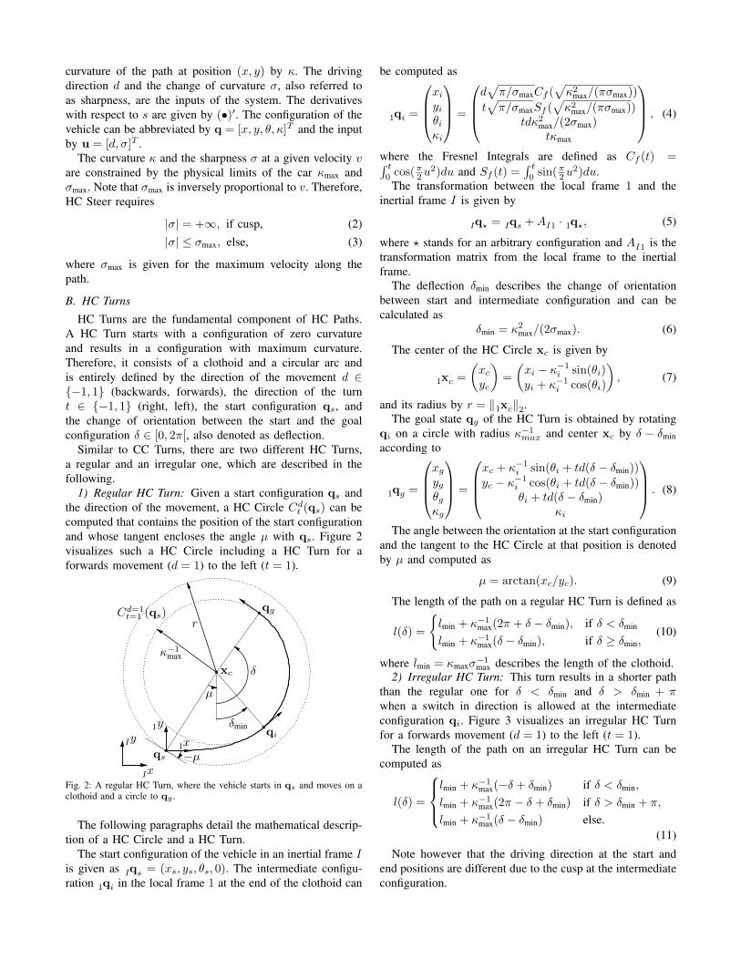
HC Turns are the fundamental component of HC Paths.A HC Turn starts with a configuration of zero curvatureand results in a configuration with maximum curvature.Therefore, it consists of a clothoid and a circular arc andis entirely defined by the direction of the movement d ∈{−1, 1} (backwards, forwards), the direction of the turnt ∈ {−1, 1} (right, left), the start configuration qs, andthe change of orientation between the start and the goalconfiguration δ ∈ [0, 2π[, also denoted as deflection.

Similar to CC Turns, there are two different HC Turns,a regular and an irregular one, which are described in thefollowing.

1) Regular HC Turn: Given a start configuration qs andthe direction of the movement, a HC Circle Cdt (qs) can becomputed that contains the position of the start configurationand whose tangent encloses the angle µ with qs. Figure 2visualizes such a HC Circle including a HC Turn for aforwards movement (d = 1) to the left (t = 1).

qg

yI

xI

y1

x1−µqs

qi

κ−1max

r

µ

δmin

δ

Cd=1t=1 (qs)

xc

Fig. 2: A regular HC Turn, where the vehicle starts in qs and moves on aclothoid and a circle to qg .

The following paragraphs detail the mathematical descrip-tion of a HC Circle and a HC Turn.

The start configuration of the vehicle in an inertial frame Iis given as qI s = (xs, ys, θs, 0). The intermediate configu-ration q1 i in the local frame 1 at the end of the clothoid can

be computed as

q1 i =

xiyiθiκi

=

d√π/σmaxCf (

√κ2max/(πσmax))

t√π/σmaxSf (

√κ2max/(πσmax))

tdκ2max/(2σmax)tκmax

, (4)

where the Fresnel Integrals are defined as Cf (t) =∫ t0cos(π2u

2)du and Sf (t) =∫ t0sin(π2u

2)du.The transformation between the local frame 1 and the

inertial frame I is given by

qI ? = qI s +AI1 · q1 ?, (5)

where ? stands for an arbitrary configuration and AI1 is thetransformation matrix from the local frame to the inertialframe.

The deflection δmin describes the change of orientationbetween start and intermediate configuration and can becalculated as

δmin = κ2max/(2σmax). (6)

The center of the HC Circle xc is given by

x1 c =

(xcyc

)=

(xi − κ−1i sin(θi)yi + κ−1i cos(θi)

), (7)

and its radius by r = ‖ x1 c‖2.The goal state qg of the HC Turn is obtained by rotating

qi on a circle with radius κ−1max and center xc by δ − δminaccording to

q1 g =

xgygθgκg

=

xc + κ−1i sin(θi + td(δ − δmin))yc − κ−1i cos(θi + td(δ − δmin))

θi + td(δ − δmin)κi

. (8)

The angle between the orientation at the start configurationand the tangent to the HC Circle at that position is denotedby µ and computed as

µ = arctan(xc/yc). (9)

The length of the path on a regular HC Turn is defined as

l(δ) =

{lmin + κ−1max(2π + δ − δmin), if δ < δmin

lmin + κ−1max(δ − δmin), if δ ≥ δmin,(10)

where lmin = κmaxσ−1max describes the length of the clothoid.

2) Irregular HC Turn: This turn results in a shorter paththan the regular one for δ < δmin and δ > δmin + πwhen a switch in direction is allowed at the intermediateconfiguration qi. Figure 3 visualizes an irregular HC Turnfor a forwards movement (d = 1) to the left (t = 1).

The length of the path on an irregular HC Turn can becomputed as

l(δ) =

lmin + κ−1max(−δ + δmin) if δ < δmin,

lmin + κ−1max(2π − δ + δmin) if δ > δmin + π,

lmin + κ−1max(δ − δmin) else.(11)

Note however that the driving direction at the start andend positions are different due to the cusp at the intermediateconfiguration.

qg

yI

xI

y1

x1−µqs

qi

κ−1max

r

µ

δmin

δ

Cd=1t=1 (qs)

xc

Fig. 3: An irregular HC Turn, where the vehicle starts in qs, moves on aclothoid to the intermediate configuration qi, switches direction, and reachesqg on a circle.

3) Comparison of RS, HC, CC Turns: In order to betterunderstand the differences between RS, HC, and CC Steer,the respective turns are compared here. Figure 4 illustrates aRS, HC, and CC Turn for a given deflection δ and Figure 5

Fig. 4: Comparison of the different turns for δ = 0.8π.

compares the turn lengths for δ ∈ [0, 2π[.

0 1 2 3 4 5 6δmin

δ [rad]

0

1

2

3

4

5

Tur

nLe

ngth

[m]

RS TurnHC TurnCC Turn

Fig. 5: Comparison of the turn lengths along a RS, HC and CC Turn withrespect to the deflection δ for κmax = 1m−1 and σmax = 1rad m−1.

It can be observed in Figure 5 that the turn lengths arelower bounded by the RS Turn for all δ. It increases linearlyuntil it reaches its peak at δ = π and decreases for largerdeflections again due to a change of the driving direction.The symmetric nature of CC Turns allows to use elementarypaths [30] for small deflections resulting in shorter turnlengths than a HC Turn. However for δ < δmin, there exists adeflection for which a HC Turn leads to a shorter turn thana CC Turn. For δ ≥ δmin, a HC Turn always results in asmaller turn length than a CC Turn because each deflection

can be reached with only one clothoid and an arc instead oftwo clothoids and an arc. Note that the nature of the irregularHC and CC Turns avoids that the turn lengths keep growingmonotonously for large deflections.

C. HC Paths

According to Reeds and Shepp, the shortest path for acar can be computed by evaluating 9 path families usingRS Turns and straight lines [6]. For paths, which includeclothoids, there exists an infinite number of possibilities toconnect two configurations [7]. Therefore, it is proposed forHC Steer to select a path with minimal length out of 13HC Families, see Table I. They consist of the RS Familiesand four additional ones based on experimental results andexperience [30].TABLE I: HC Families: C denotes a turn, S a straight line, and | a cusp.

RS Families Additional Families

C|C|C CCCC|CC C|SCCC|C CS|CCSC C|S|CCC|CCC|CC|CC|CSCCSC|CC|CSC|C

HC Paths provide the flexibility to start and end withzero curvature, in the following denoted as HC00, or withmaximum curvature ±κmax denoted as HC±±. Compared toHC00, HC±± Steer leaves the initial and final clothoid awayresulting in shorter paths, see Subsection IV-D. The nextparagraph outlines the general procedure for computing theHC Families and explicitly details the computation of HC00

Steer for the family C|C|C.For every HC Family and two given configurations qs

and qg , a path can be computed in four steps: (1) Fit 4 startand 4 goal HC Circles (forwards/backwards, left/right) tothe given configurations. (2) Out of the 4 · 4 possibilities toconnect qs and qg , remove the combinations that can not berealized by the corresponding family. For instance in caseof C|C|C, the HC Circle Cd=1

t=1 (qs) always requires the HCCircle Cd=−1t=1 (qg) at the goal configuration, see Figure 6.(3) For every resulting combination, use RS, HC, CC Turns,

qg

κ−1max

κ−1max

κ−1max

Cd=1t=1 (qs)

Cd=−1t=1 (qg)

qs

distxc,1

xc,3

xc,2

h

xI

yI

x1

y1

Fig. 6: Illustration of a HC00 Path for a C|C|C family and the two HCCircles Cd=1

t=1 (qs) and Cd=−1t=1 (qg).

and tangency conditions to connect start and goal HC Circleby enforcing curvature continuity between cusps. In case ofC|C|C, this is shown in Figure 6, where a RS Turn is usedto connect the start and goal HC Circle. The center of theRS Turn xc,2 in the local frame can then be computed as

h =

√(4κ−2max −

1

4dist2(xc,1,xc,3)), (12)

x1 c,2 =

(12dist(xc,1,xc,3)

h

), (13)

where the symbols correspond to Figure 6. (4) Finally selectthe start and goal HC Circle that results in the shortest pathfor the corresponding family.

D. Comparison of RS, HC, CC Steer

This subsection evaluates and compares HC Steer with RSand CC Steer in terms of path length and computation time.

Figure 7 illustrates the relative difference in path length ofHC±±, HC00, and CC Steer compared to RS Steer for 105

random steering procedures.

0.0 10.0 20.0 30.0 40.0

Rel. Difference in Path Length to RS Steer [%]

0.0

10.0

20.0

30.0

40.0

50.0

60.0

Normalized

Frequency[%

]

HC±±

HC00

CC

Fig. 7: Relative difference in path length of HC±±, HC00, and CCSteer compared to RS Steer for 105 randomly sampled start and goalconfigurations (κmax = 1m−1, σmax = 1 rad m−1).

While CC Steer generates the largest deviations from RSSteer, HC±± Steer generates paths that deviate in more than60% less than 2.5% from the length of RS Paths. Thisshows HC±± Steer’s capability of approximating RS Steerwhile maintaining curvature continuity between cusps. Theperformance of HC00 Steer lies between HC±± and CCSteer.

The computation times of the different steering func-tions are evaluated on a single core of an Intel XeonE5@3.50GHz, 10MB cache, and listed in Table II. It can beobserved that the curvature continuity comes at a cost of upto 13 times longer computations. RS Paths can be computedTABLE II: Comparison of the computation time of RS, HC00, HC±±, andCC Steer for 105 random steering procedures.

computation time

mean [µs] std [µs]

RS 6.9 ±1.3HC00 89.5 ±10.5HC±± 89.1 ±15.0CC 79.0 ±11.5

on average in 6.9 µs. HC00 and HC±± Steer perform almost

equally and find solutions on average in less than 89.5 µs.The computation of CC Steer is slightly faster and takes onaverage 79.0 µs. Standard deviations are below 15.0 µs forall analyzed steering functions.

As shown in Section VI, the longer computations havea minor effect on the overall runtime when integrated intoBiRRT* since most of the computation time is spent in thecollision checker.

E. Topological Admissibility

RS, HC, and CC Steer always find a connecting pathfor two random configurations making all three steeringfunctions complete. In order to guarantee that these methodsalso result in a collision free, (probabilistically) completepath when integrated into a general motion planner likeBiRRT*, they have to be topologically admissible [31], [7]:

∀ε > 0,∃η > 0,∀(qs,qg) ∈ C2,qg ∈ B(qs, η)⇒ steer(qs,qg) ⊂ B(qs, ε),

(14)

where B(q, •) describes a ball of a given size centeredat configuration q, and steer(qs,qg) denotes a steeringprocedure.

Equation (14) states that a steering function is topo-logically admissible if the computed path stays in an ε-neighborhood when start and goal configurations are locatedin an η-neighborhood. By nature, RS Steer fulfills this con-dition since its paths only consist of straight lines and circleswithout a minimal required path length. In contrast to that,CC Steer is only topologically admissible when additionalso-called topological paths are introduced [7]. Similar to CCSteer, HC00 Steer also requires additional topological pathsfor completeness in a general motion planner. The reason isthat the clothoids at the start and goal configuration resultin path lengths that are always lower bounded by 2lmin.Experiments have shown however that these topologicalpaths are only a theoretical construct and not practical inreality. This is because the nature of the clothoids in thetopological paths allows only small η-neighborhoods fora moderate ε limiting the maneuverability of the vehiclesignificantly.

In contrast to CC and HC00 Steer, HC±± Steer is topo-logically admissible. This is due to the fact that the familiesC|C|C and C|S|C in HC±± Steer only consist of circlesand straight lines (HC±± starts and ends with maximumcurvature). The absence of clothoids allows to generate paths,whose length is not lower bounded anymore. Therefore,HC±± Steer results in completeness when integrated intoa general motion planner.

V. PLANNING WITH BIRRT*

In order to compute a collision-free, asymptotically op-timal path, BiRRT* requires a collision checker and acost function for minimization. This section introduces theimplemented collision checker in Subsection V-A and thechosen cost function in Subsection V-B.

A. Collision Checking

Designing a fast collision checker is essential sinceBiRRT* spends most of its computation time checking treeextensions for collisions with the environment. Currently, itis assumed that the environment is static and that obstacle i,labeled as Oi, is given as a convex polygon. For non-convexshapes, this can be achieved by a convex decomposition [32].Note that in the following, a calligraphic letter is usedwhenever a set of points occupied by an object is described.

At every discrete configuration q along the path, the bodyof the ego vehicle A1 and all actuated tires j, labeled asTj , are checked in two consecutive steps for collision withthe entire environment. This setup is illustrated in Figure 8,where the body’s circumscribed circle is denoted as A2 andA1,A2,Oi, Tj ⊂ R2.

O1

O2

O3

A2(q)

T1(q)

T2(q)

yI

xI

A1(q)

q

Fig. 8: Illustration of the ego vehicle’s body A1, the car body’s circum-scribed circle A2, its actuated tires Tj at configuration q, and the obstaclesOi in the environment.

In the first step of the collision check, obstacle Oi islabeled as a collision hypothesis Hi if

A2(q) ∩ Oi 6= ∅, (15)

where A2(q) describes the car body’s circumscribed circle atconfiguration q. In the second step, all collision hypothesesare checked against the body of the car A1 and its actu-ated tires Tj at configuration q. Collision hypothesis Hi iscollision-free if

A1(q) ∩Hi = ∅ ∧ Tj(q) ∩Hi = ∅, ∀j. (16)

We use the Gilbert-Johnson-Keerthi (GJK) algorithm [33]to perform the second step of the collision check. The GJKalgorithm takes on average 700 ns for a binary collisioncheck of two polygons each consisting of 23 vertices on asingle core of an Intel Xeon E5@3.50GHz, 10MB cache. Itis also capable of computing the minimal distance betweentwo polygons if they are not colliding, which takes onaverage additional 300 ns.

B. Cost Function

The cost function J is evaluated along the path, which isgiven by N segments, see Figure 9. It consists of four terms,computes a positive cost for every non-trivial path [34], andis given as

J = wTJ

JlengthJcuspJcurvJobs

, (17)

s

(sk,qk,uk)(sk+1,qk+1,uk+1)

Fig. 9: Illustration of the kth path segment connecting configuration qk andqk+1. The arc length along the path is described by s and uk,uk+1 denotethe inputs at distance sk and sk+1, respectively.

where wJ allows to weight each cost term, Jlength penalizesthe length of the path, Jcusp punishes cusps in the path,Jcurv makes uncomfortable paths in terms of curvature moreexpensive, and Jobs puts a cost on paths with little clearanceto static obstacles.

The cost terms are computed as

Jlength =

∫ sN

s0

ds, (18)

Jcusp =

N−1∑k=0

1dk+1·dk<0, (19)

Jcurv = (κmax(sN − s0))−1∫ sN

s0

|κ(s)|ds, (20)

Jobs = 1− mins∈[s0,sN ]

(dobs(s), dsafety,1)

/dsafety,1, (21)

where the driving direction at distance sk is denoted as dk,the minimal clearance along the path as dobs, and the softsafety distance as dsafety,1. Equation (18) computes the lengthof the path while equation (19) counts the cusps in the path.Equation (20) integrates and normalizes the curvature alongthe path, and equation (21) compares the minimal clearanceof the path with the soft safety distance, also see [15].

VI. EXPERIMENTS

The experimental results analyze and compare the per-formance of BiRRT* with RS, HC±±, and CC1 Steer ontwo different HDP scenarios.2 Figure 10 visualizes the twoscenarios.

Fig. 10: Scenario I (left) and scenario II (right), where the gray shaded areamarks the region that is excluded from the sampling region of BiRRT*.

The setup used in the experiments is described in Subsec-tion VI-A, and Subsection VI-B discusses the results.

A. Setup

The width of the driveway is given by wD = 5.5m, thewidth and length of a parking spot by wS = 2.5m and lS =

1CC Steer is used without topological paths as explained in Section IV-E.2This link https://youtu.be/RlZZ4jnEhTM provides a video of

the results, and the source code of the steering functions is available athttps://github.com/hbanzhaf/steering_functions.

5m according to the national standards in Germany [35]. Inorder to analyze how the proposed motion planner performsin each scenario, the experiments incrementally increase thelength lD in the driveway.

As it can be seen in Figure 1, the vehicles in the environ-ment, which consist of commercially available mid-size andfull-size cars, are given by their convex hull. Each is inflatedby a hard safety distance of dsafety,2 = 10 cm. The hard safetydistance shrinks the available space for maneuvering sincelD describes the actual distance between the car bodies. Anadditional 20 cm is added as a soft safety distance dsafety,1,see Subsection V-B.

The ego vehicle’s parameters are listed in Table III, whereκmax and σmax already include 10% control reserve. The max.sharpness is given at a longitudinal velocity of 1m s−1.

TABLE III: Vehicle parameters

Parameter Symbol Value

Length - 4.926mWidth - 2.086mWheel Base L 2.912mMax. Curvature κmax 1/4.994m−1

Max. Sharpness σmax 0.315 rad m−1

The planner BiRRT* is executed for 6 s by uniformlysampling configurations in the operating region, which can beseen in Figure 10 (21m× 5.5m in scenario I, 21m× 18min scenario II, and [0, 2π[ for the heading angle in bothscenarios). A goal sampling frequency of 5% is applied,collision checks are performed every 10 cm, and the constantγ [26] is set to 6.0. To mitigate randomization effects, everyexperiment is repeated 100 times with the same setup. Theextend procedures in BiRRT* are selected as RS, CC, andHC±± Steer due to its topological admissibility.

The proposed motion planner is implemented as ROS nodein C++ based on [36] and executed on a single core of anIntel Xeon E5@3.50GHz, 10MB cache.

B. Results

The results with regard to lD, namely the time to firstsolution tTTFS, the number of curvature discontinuities, thenumber of cusps, the path length, and the success rateof finding a solution after 100 repetitions of the sameexperiment, are given in Table IV. Note that BiRRT* grows atree from start to goal and vice versa and therefore performsequally for maneuvering in and out of the parking spot.

Based on Table IV, Figure 11 illustrates the time to firstsolution tTTFS and the success rate relating to lD in scenario I.

BiRRT* with RS and HC±± Steer finds solutions for lD ≥5.6m in scenario I while CC Steer requires an additional80 cm. In scenario II, solutions are generated with RS andHC±± Steer for lD ≥ 4.0m, and lD ≥ 4.6m for CC Steer.

Overall the average time to first solution, the number ofcurvature discontinuities, and the number of cusps decreasewhen lD is increased while the success rate raises, alsosee Figure 11. RS Steer mostly results in slightly fastersolutions with less cusps and higher success rates than HC±±

5.6 5.8 6.0 6.2 6.4 6.6

lD [m]

0

1

2

3

4

5

t TTFS

[s]

RSHC±±

CC

Fig. 11: Comparison of BiRRT*’s performance with RS, HC±±, and CCSteer by measuring the time to first solution tTTFS with respect to lD inscenario I. The size of the visualized markers indicates the success rate infinding a path within 6 s.

Steer. However, Table IV shows that RS Steer’s paths sufferfrom more than twice as many curvature discontinuities thanHC±± Steer’s paths because HC±± Steer enforces κ to becontinuous between cusps, see Figure 12. Consequently, the

0.0 2.5 5.0 7.5 10.0 12.5 15.0

s [m]

−0.2

0.0

0.2

κ[1

/m] κ

d

−1

0

1

d[-]

Fig. 12: Curvature κ along a solution path in scenario II when maneuveringinto the parking spot (lD = 4.8m) with BiRRT* and HC±± Steer. Thedriving direction at a given arc length s is given by d.

resulting paths of HC±± Steer are more comfortable to driveand easier to be tracked by a controller than the curvaturediscontinuous paths of RS Steer.

Compared to CC Steer, HC±± Steer computes solutionsfaster, leaving BiRRT* more time for optimizing the initiallygenerated path. Additionally, it outperforms CC Steer interms of number of cusps and success rate.

VII. CONCLUSION AND OUTLOOK

In this paper, a novel extend function called HybridCurvature (HC) Steer for sampling-based nonholonomic mo-tion planning in tight environments is introduced. HC Steerapproximates Reeds-Shepp’s paths in terms of path length,but enforces curvature continuity between cusps resulting indirectly drivable paths for nonholonomic systems. Experi-ments in tight environments with the optimal motion plannerBiRRT* show HC Steer’s advantage of computing smootherpaths than RS Steer in equally challenging environments.Compared to CC Steer, HC Steer with BiRRT* finds solu-tions with less direction switches, shorter planning time, andhigher success rates. Hence HC Steer clearly outperformsboth RS and CC Steer from a practical point of view.

In the future, we aim to combine the proposed HC±±

steering function with HC0± and HC±0 Steer, which startor end with either zero or maximal curvature. Such a com-bination would allow to generate paths with preferably zero

TABLE IV: Results of BiRRT* in Scenario I/II after 6 s of sampling time and 100 repetitions of the same experiment. The time to first solution tTTFS, thenumber of curvature discontinuities, the number of cusps, the path lengths, and success rates are listed with respect to lD. Mean path lengths are rounded.

tTTFS (mean± std) [s] #curv. discon. (mean± std) [−] #cusps (mean± std) [−] length (mean± std) [m] success rate [%]

lD [m] RS HC±± CC RS HC±± CC RS HC±± CC RS HC±± CC RS HC±± CC

Scen

ario

I

5.4 - - - - - - - - - - - - 0 0 05.6 3.3±1.4 4.9±0.9 - 12.5±2.7 6.8±1.8 - 6.4±1.5 9.1±2.1 - 14±1.7 17±3.8 - 50 13 05.8 1.1±1.0 2.9±1.6 - 10.2±3.1 4.6±1.5 - 4.6±1.4 6.7±2.5 - 14±3.5 17±3.9 - 100 90 06.0 0.3±0.2 0.9±0.7 - 8.3±2.3 3.2±1.1 - 3.4±1.0 4.7±1.8 - 13±1.5 15±2.3 - 100 100 06.2 0.1±0.1 0.4±0.3 - 7.7±2.4 2.3±1.2 - 2.3±1.1 3.5±1.7 - 14±2.1 15±2.8 - 100 100 06.4 0.1±0.1 0.2±0.2 2.4±0.7 6.7±2.1 1.8±0.9 0±0 1.7±0.9 2.6±1.3 4.5±0.5 13±1.3 14±2.3 16±0.1 100 100 26.6 0.1±0.1 0.2±0.2 1.2±0.8 6.5±1.9 1.5±0.9 0±0 1.5±0.8 2.2±1.5 4.7±1.7 13±1.5 14±3.3 18±3.1 100 100 100

Scen

ario

II

3.8 - - - - - - - - - - - - 0 0 04.0 2.7±1.4 5.1±0.7 - 13.4±3.6 4.0±0.0 - 6.2±1.8 5.0±0.0 - 18±3.3 21±0.9 - 12 2 04.2 2.5±1.5 3.6±1.7 - 12.9±2.6 4.4±0.7 - 5.7±1.4 6.5±2.1 - 18±3.2 23±2.0 - 50 13 04.4 1.9±1.3 2.6±1.6 - 11.8±2.4 3.2±1.0 - 4.6±1.4 5.5±1.8 - 18±4.9 21±4.4 - 85 51 04.6 1.3±1.3 2.2±1.5 3.1±1.7 10.4±2.3 2.9±1.3 0±0 3.6±1.5 4.9±2.0 6.5±1.7 17±2.8 22±3.1 20±3.0 95 75 44.8 0.6±0.6 1.7±1.2 3.4±2.0 9.6±2.1 2.5±0.9 0±0 3.1±1.2 4.1±1.3 5.1±1.5 16±1.9 21±4.0 19±2.5 100 97 215.0 0.5±0.5 1.0±1.0 3.2±1.6 9.3±1.8 2.4±0.8 0±0 3.0±1.1 4.0±1.6 5.2±2.0 16±2.1 21±3.4 20±5.4 100 98 645.2 0.3±0.2 0.8±0.7 1.6±1.4 8.5±1.9 2.3±0.8 0±0 2.5±0.9 3.7±1.2 4.1±1.6 16±1.5 20±3.2 18±2.9 100 100 925.4 0.2±0.2 0.6±0.5 1.0±0.9 8.5±1.6 2.1±0.7 0±0 2.3±0.7 3.2±1.0 3.2±1.3 15±1.1 19±3.2 17±2.4 100 100 100

curvature at the beginning and at the end while still providingthe desirable characteristics of HC±± Steer in between.

REFERENCES

[1] (2017) Bosch and Daimler demonstrate driverless parking in real-lifeconditions. Robert Bosch GmbH. (visited on 2017/07/26). [Online].Available: http://http://www.bosch-presse.de/pressportal/de/en/news/

[2] H. Banzhaf et al., “The Future of Parking: A Survey on AutomatedValet Parking with an Outlook on High Density Parking,” in IEEEIntelligent Vehicles Symposium, 2017.

[3] H. Banzhaf et al., “High Density Valet Parking Using k-Deques inDriveways,” in IEEE Intelligent Vehicles Symposium, 2017.

[4] G. Schildbach and F. Borrelli, “A Dynamic Programming Approachfor Nonholonomic Vehicle Maneuvering in Tight Environments,” inIEEE Intelligent Vehicles Symposium, 2016.

[5] D. Kim et al., “Practical motion planning for car-parking control innarrow environment,” IET Control Theory & Applications, 2010.

[6] J. Reeds and L. Shepp, “Optimal paths for a car that goes bothforwards and backwards,” Pacific Journal of Mathematics, 1990.

[7] T. Fraichard and A. Scheuer, “From Reeds and Shepp’s to Continuous-Curvature Paths,” IEEE Transactions on Robotics, 2004.

[8] M. Jordan and A. Perez, “Optimal Bidirectional Rapidly-ExploringRandom Trees,” CSAIL, MIT, Cambridge, MA, TR 2013-021, 2013.

[9] D. Gonzalez et al., “A Review of Motion Planning Techniques forAutomated Vehicles,” IEEE Transactions on Intelligent TransportationSystems, 2016.

[10] B. Paden et al., “A Survey of Motion Planning and Control Techniquesfor Self-driving Urban Vehicles,” IEEE Transactions on IntelligentVehicles, 2016.

[11] M. Likhachev and D. Ferguson, “Planning Long Dynamically-FeasibleManeuvers for Autonomous Vehicles,” The International Journal ofRobotics Research, 2009.

[12] D. Dolgov et al., “Path Planning for Autonomous Vehicles in Un-known Semi-structured Environments,” The International Journal ofRobotics Research, 2010.

[13] C. Siedentop et al., “Path-Planning for Autonomous Parking withDubins Curves,” in Uni-DAS Workshop Fahrerassistenzsysteme, 2015.

[14] J. Ziegler, M. Werling, and J. Schroder, “Navigating car-like Robots inunstructured Environments using an Obstacle sensitive Cost Function,”in IEEE Intelligent Vehicles Symposium, 2008.

[15] U. Schwesinger et al., “Vision-Only Fully Automated Driving inDynamic Mixed-Traffic Scenarios,” it-Information Technology, 2015.

[16] J. hwan Jeon et al., “Anytime Computation of Time-Optimal Off-RoadVehicle Maneuvers using the RRT*,” in IEEE Conference on Decisionand Control and European Control Conference, 2011.

[17] J. hwan Jeon et al., “Optimal Motion Planning with the Half-CarDynamical Model for Autonomous High-Speed Driving,” in IEEEAmerican Control Conference, 2013.

[18] S. Klemm et al., “RRT*-Connect: Faster, Asymptotically OptimalMotion Planning,” in IEEE International Conference on Robotics andBiomimetics, 2015.

[19] S. Karaman and E. Frazzoli, “Incremental Sampling-based Algorithmsfor Optimal Motion Planning,” Robotics Science and Systems VI, 2010.

[20] H. Vorobieva et al., “Automatic Parallel Parking with GeometricContinuous-Curvature Path Planning,” in IEEE Intelligent VehiclesSymposium, 2014.

[21] J. Schulman et al., “Motion Planning with Sequential Convex Opti-mization and Convex Collision Checking,” The International Journalof Robotics Research, 2014.

[22] P. Zips et al., “Optimisation based path planning for car parking innarrow environments,” Robotics and Autonomous Systems, 2016.

[23] J. Ziegler et al., “Trajectory Planning for Bertha - a Local, ContinuousMethod,” in IEEE Intelligent Vehicles Symposium, 2014.

[24] S. M. LaValle, “Rapidly-Exploring Random Trees: A New Tool forPath Planning,” Tech. Rep., 1998.

[25] Y. Kuwata et al., “Real-time Motion Planning with Applications toAutonomous Urban Driving,” IEEE Transactions on Control SystemsTechnology, 2009.

[26] S. Karaman and E. Frazzoli, “Optimal Kinodynamic Motion Planningusing Incremental Sampling-based Methods,” in IEEE Conference onDecision and Control, 2010.

[27] D. J. Webb and J. van den Berg, “Kinodynamic RRT*: AsymptoticallyOptimal Motion Planning for Robots with Linear Dynamics,” in IEEEInternational Conference on Robotics and Automation, 2013.

[28] L. E. Dubins, “On Curves of Minimal Length with a Constraint onAverage Curvature, and with Prescribed Initial and Terminal Positionsand Tangents,” American Journal of Mathematics, 1957.

[29] R. Rajamani, Vehicle Dynamics and Control. Springer Science, 2011.[30] A. Scheuer and T. Fraichard, “Continuous-Curvature Path Planning for

Car-Like Vehicles,” in IEEE International Conference on IntelligentRobots and Systems, 1997.

[31] S. Sekhavat and J.-P. Laumond, “Topological Property for Collision-Free Nonholonomic Motion Planning: The Case of Sinusoidal Inputsfor Chained Form Systems,” IEEE Transactions on Robotics andAutomation, 1998.

[32] C. Ericson, Real-Time Collision Detection. CRC Press, 2004.[33] E. G. Gilbert, D. W. Johnson, and S. S. Keerthi, “A Fast Procedure

for Computing the Distance Between Complex Objects in Three-Dimensional Space,” IEEE Journal on Robotics and Automation, 1988.

[34] S. Karaman and E. Frazzoli, “Sampling-based Optimal Motion Plan-ning for Non-holonomic Dynamical Systems,” in IEEE InternationalConference on Robotics and Automation, 2013.

[35] “Verordnung des Ministeriums fur Verkehr und Infrastruktur uberGaragen und Stellplatze,” §4 Stellplatze und Fahrgassen, Frauen-parkplatze, Ministerium fur Verkehr und Infrastruktur, 1997.

[36] S. Karaman. (2017) SMP Library. (visited on 2017/03/24). [Online].Available: https://svn.csail.mit.edu/smp