HW4, Math 322, Fall 2016

Nasser M. Abbasi

December 30, 2019

Contents

1 HW 4 21.1 Problem 2.5.24 . . . . . . . . . . . . . . . . . . . . . . . . . . . . . . . . . . . . . . . . . 21.2 Problem 3.2.2 (b,d) . . . . . . . . . . . . . . . . . . . . . . . . . . . . . . . . . . . . . . . 4

1.2.1 Part b . . . . . . . . . . . . . . . . . . . . . . . . . . . . . . . . . . . . . . . . . . 41.2.2 Part d . . . . . . . . . . . . . . . . . . . . . . . . . . . . . . . . . . . . . . . . . . 9

1.3 Problem 3.2.4 . . . . . . . . . . . . . . . . . . . . . . . . . . . . . . . . . . . . . . . . . . 131.4 Problem 3.3.2 (d) . . . . . . . . . . . . . . . . . . . . . . . . . . . . . . . . . . . . . . . . 131.5 Problem 3.3.3 (b) . . . . . . . . . . . . . . . . . . . . . . . . . . . . . . . . . . . . . . . . 161.6 Problem 3.3.8 . . . . . . . . . . . . . . . . . . . . . . . . . . . . . . . . . . . . . . . . . . 19

1.6.1 Part (a) . . . . . . . . . . . . . . . . . . . . . . . . . . . . . . . . . . . . . . . . . 191.6.2 Part (b) . . . . . . . . . . . . . . . . . . . . . . . . . . . . . . . . . . . . . . . . . 191.6.3 Part (c) . . . . . . . . . . . . . . . . . . . . . . . . . . . . . . . . . . . . . . . . . 19

1.7 Problem 3.4.3 . . . . . . . . . . . . . . . . . . . . . . . . . . . . . . . . . . . . . . . . . . 211.7.1 Part (a) . . . . . . . . . . . . . . . . . . . . . . . . . . . . . . . . . . . . . . . . . 211.7.2 Part (b) . . . . . . . . . . . . . . . . . . . . . . . . . . . . . . . . . . . . . . . . . 23

1.8 Problem 3.4.9 . . . . . . . . . . . . . . . . . . . . . . . . . . . . . . . . . . . . . . . . . . 251.9 Problem 3.4.11 . . . . . . . . . . . . . . . . . . . . . . . . . . . . . . . . . . . . . . . . . 26

1

2

1 HW 4

1.1 Problem 2.5.24

88

(a) 8' (x, 0) = 0,

(b) u(x,0) = 0,

(c) u(x,0) = 0,

(d) (x, 0) = 0,

Chapter 2. Method of Separation of Variables

"' (x, H) = 0, u(0, y) = f (y)

u(x, H) = 0, u(0,y) = f(y)

u(x, H) = 0, (0,y) = f(y)

Ou (x, H) = 0, a: (0, y) = f (y)

Show that the solution [part (d)] exists only if fH f (y) dy = 0.

2.5.16. Consider Laplace's equation inside a rectangle 0 < x < L, 0 < y < H, withthe boundary conditions

8uau

8u&"

8x(0,y) = 0, 8x(L, y) = g(y),

8y(x, 0)= 0, 8y (x, H) = f (x)

(a) What is the solvability condition and its physical interpretation?(b) Show that u(x, y) = A(x2 - y2) is a solution if f (x) and g(y) are

constants [under the conditions of part (a)].(c) Under the conditions of part (a), solve the general case [nonconstant

f (x) and g(y)]. [Hints: Use part (b) and the fact that f (x) = f +[f (x) - f.,.], where f.,. = L fL f (x) dx.]

2.5.17. Show that the mass density p(x, t) satisfies k + V (pu) = 0 due to con-servation of mass.

2.5.18. If the mass density is constant, using the result of Exercise 2.5.17, showthat

2.5.19. Show that the streamlines are parallel to the fluid velocity.

2.5.20. Show that anytime there is a stream function, V x u = 0.

2.5.21. From u and v=- ,derive u,-=rue=-2.5.22. Show the drag force is zero for a uniform flow past a cylinder including

circulation.

2.5.23. Consider the velocity ug at the cylinder. Where do the maximum andminimum occur?

2.5.24. Consider .the velocity ue at the cylinder. If the circulation is negative, showthat the velocity will be larger above the cylinder than below.

2.5.25. A stagnation point is a place where u = 0. For what values of the circulationdoes a stagnation point exist on the cylinder?

2.5.26. For what values of 0 will u,. = 0 off the cylinder? For these 6, where (forwhat values of r) will ue = 0 also?

2.5.27. Show that r/ = a 81T B satisfies Laplace's equation. Show that the streamlinesare circles. Graph the streamlines.

Introduction. The stream velocity �� in Cartesian coordinates is

�� = 𝑢 𝚤 + 𝑣 𝚥

=𝜕Ψ𝜕𝑦

𝚤 −𝜕Ψ𝜕𝑥

𝚥 (1)

Where Ψ is the stream function which satisfies Laplace PDE in 2D ∇ 2Ψ = 0. In Polar coordinatesthe above becomes

�� = 𝑢𝑟�� + 𝑢𝜃��

=1𝑟𝜕Ψ𝜕𝜃

�� −𝜕Ψ𝜕𝑟

�� (2)

The solution to ∇ 2Ψ = 0 was found under the following conditions

1. When 𝑟 very large, or in other words, when too far away from the cylinder or the wing, theflow lines are horizontal only. This means at 𝑟 = ∞ the 𝑦 component of �� in (1) is zero. This

means𝜕Ψ�𝑥,𝑦�

𝜕𝑥 = 0. Therefore Ψ�𝑥, 𝑦� = 𝑢0𝑦 where 𝑢0 is some constant. In polar coordinates thisimplies Ψ(𝑟, 𝜃) = 𝑢0𝑟 sin𝜃, since 𝑦 = 𝑟 sin𝜃.

2. The second condition is that radial component of �� is zero. In other words, 1𝑟𝜕Ψ𝜕𝜃 = 0 when

𝑟 = 𝑎, where 𝑎 is the radius of the cylinder.

3. In addition to the above two main condition, there is a condition that Ψ = 0 at 𝑟 = 0

Using the above three conditions, the solution to ∇ 2Ψ = 0 was derived in lecture Sept. 30, 2016, tobe

Ψ(𝑟, 𝜃) = 𝑐1 ln � 𝑟𝑎� + 𝑢0 �𝑟 −

𝑎2

𝑟 �sin𝜃

Using the above solution, the velocity �� can now be found using the definition in (2) as follows

1𝑟𝜕Ψ𝜕𝜃

=1𝑟𝑢0 �𝑟 −

𝑎2

𝑟 �cos𝜃

𝜕Ψ𝜕𝑟

=𝑐1𝑟+ 𝑢0 �1 +

𝑎2

𝑟2 �sin𝜃

Hence, in polar coordinates

�� = � 1𝑟𝑢0 �𝑟 −𝑎2

𝑟� cos𝜃� �� − � 𝑐1𝑟 + 𝑢0 �1 +

𝑎2

𝑟2� sin𝜃� �� (3)

3

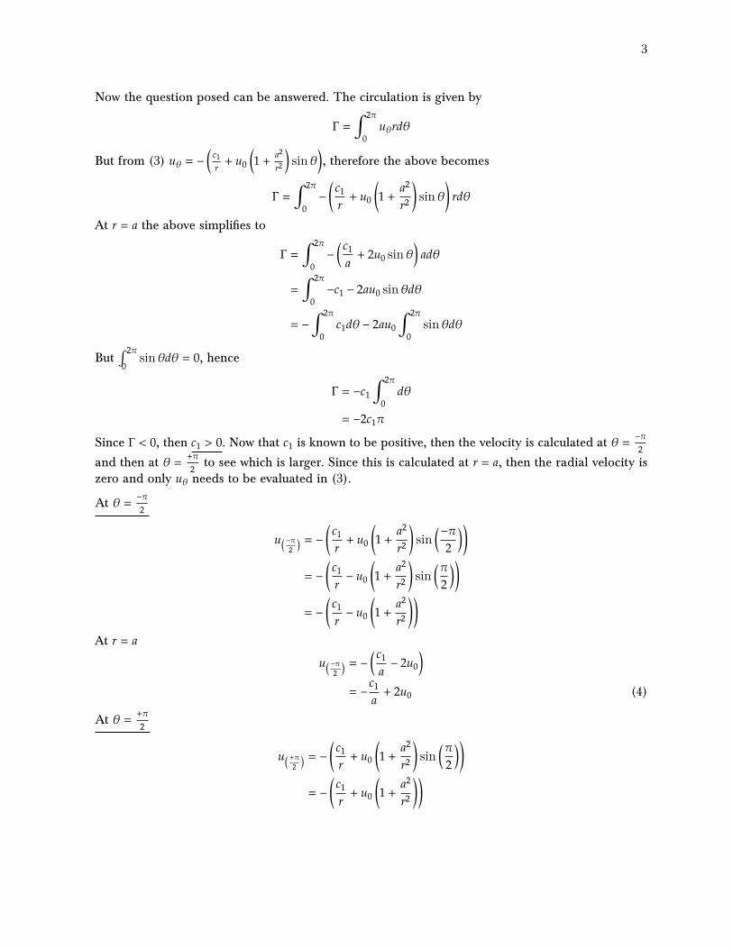
Now the question posed can be answered. The circulation is given by

Γ = �2𝜋

0𝑢𝜃𝑟𝑑𝜃

But from (3) 𝑢𝜃 = − �𝑐1𝑟 + 𝑢0 �1 +

𝑎2

𝑟2� sin𝜃�, therefore the above becomes

Γ = �2𝜋

0− �𝑐1𝑟+ 𝑢0 �1 +

𝑎2

𝑟2 �sin𝜃� 𝑟𝑑𝜃

At 𝑟 = 𝑎 the above simplifies to

Γ = �2𝜋

0− �𝑐1𝑎+ 2𝑢0 sin𝜃� 𝑎𝑑𝜃

= �2𝜋

0−𝑐1 − 2𝑎𝑢0 sin𝜃𝑑𝜃

= −�2𝜋

0𝑐1𝑑𝜃 − 2𝑎𝑢0�

2𝜋

0sin𝜃𝑑𝜃

But ∫2𝜋

0sin𝜃𝑑𝜃 = 0, hence

Γ = −𝑐1�2𝜋

0𝑑𝜃

= −2𝑐1𝜋

Since Γ < 0, then 𝑐1 > 0. Now that 𝑐1 is known to be positive, then the velocity is calculated at 𝜃 = −𝜋2

and then at 𝜃 = +𝜋2 to see which is larger. Since this is calculated at 𝑟 = 𝑎, then the radial velocity is

zero and only 𝑢𝜃 needs to be evaluated in (3).

At 𝜃 = −𝜋2

𝑢� −𝜋2 � = − �𝑐1𝑟+ 𝑢0 �1 +

𝑎2

𝑟2 �sin �−𝜋

2��

= − �𝑐1𝑟− 𝑢0 �1 +

𝑎2

𝑟2 �sin �𝜋

2��

= − �𝑐1𝑟− 𝑢0 �1 +

𝑎2

𝑟2 ��

At 𝑟 = 𝑎

𝑢� −𝜋2 � = − �𝑐1𝑎− 2𝑢0�

= −𝑐1𝑎+ 2𝑢0 (4)

At 𝜃 = +𝜋2

𝑢�+𝜋2 � = − �𝑐1𝑟+ 𝑢0 �1 +

𝑎2

𝑟2 �sin �𝜋

2��

= − �𝑐1𝑟+ 𝑢0 �1 +

𝑎2

𝑟2 ��

4

At 𝑟 = 𝑎

𝑢� −𝜋2 � = − �𝑐1𝑎+ 2𝑢0�

= −𝑐1𝑎− 2𝑢0 (5)

Comparing (4),(5), and since 𝑐1 > 0, then the magnitude of 𝑢𝜃 at 𝜋2 is larger than the magnitude of

𝑢𝜃 at −𝜋2 . Which implies the stream flows faster above the cylinder than below it.

1.2 Problem 3.2.2 (b,d)

3.2. Convergence Theorem

L n7rx L n7rx n7rxan

Lf (x) cos L dx = L J cos L dx nir sin L

L L/2

= 1sinn7r - sin

nirnir 2

bn = 1 L f (x) sinnirx

L

1Ldx = sin n

xL nir LLJ

/2

nnCos - - cos n7r

n7r 2

95

(3.2.7)

(3.2.8)

We omit simplifications that arise by noting that sinn7r = 0, cosnir = (-1)", andso on.

EXERCISES 3.2

3.2.1. For the following functions, sketch the Fourier series off (x) (on the interval-L < x < L). Compare f (x) to its Fourier series:

(a) f(x) = 1 *(b) f(x) = x2

(c) f(x)=1+x *(d) f(x) = ex

(e) f (x) = { 2x x > 0 * (f) f (x) 1+x(g) f(x) x

0x < L/2x > L/2

x > O

3.2.2. For the following functions, sketch the Fourier series of f (x) (on the interval-L < x < L) and determine the Fourier coefficients:

*(a) f(x)=x (b) f(x) = e-x

*(c) f(x) = sin

L(d) f(x)

0 x < 0

l x x>0

(e) f(x) I jxj < L/20 jxI > L/2

(g) f(x) = I 1 x < 0

l 2 x>0

-1 nirxdx = - cos

* (f) f (x) = l 0

L

IL/2

L

L/2

x<0x>0

1.2.1 Part b

The following is sketch of periodic extension of 𝑒−𝑥 from 𝑥 = −𝐿⋯𝐿 (for 𝐿 = 1) for illustration. Thefunction will converge to 𝑒−𝑥 between 𝑥 = −𝐿⋯𝐿 and between 𝑥 = −3𝐿⋯− 𝐿 and between 𝑥 = 𝐿⋯3𝐿and so on. But at the jump discontinuities which occurs at 𝑥 = ⋯ ,−3𝐿, −𝐿, 𝐿, 3𝐿,⋯ it will converge tothe average shown as small circles in the sketch.

oo o o

-3 -2 -1 1 2 3

0.5

1.0

1.5

2.0

2.5

3.0

Periodic extension of exp(-x) from -1...1

5

By definitions,

𝑎0 =1𝑇 �

𝑇/2

−𝑇/2𝑓 (𝑥) 𝑑𝑥

𝑎𝑛 =1𝑇/2 �

𝑇/2

−𝑇/2𝑓 (𝑥) cos �𝑛 �

2𝜋𝑇 �

𝑥� 𝑑𝑥

𝑏𝑛 =1𝑇/2 �

𝑇/2

−𝑇/2𝑓 (𝑥) sin �𝑛 �

2𝜋𝑇 �

𝑥� 𝑑𝑥

The period here is 𝑇 = 2𝐿, therefore the above becomes

𝑎0 =12𝐿 �

𝐿

−𝐿𝑓 (𝑥) 𝑑𝑥

𝑎𝑛 =1𝐿 �

𝐿

−𝐿𝑓 (𝑥) cos �𝑛𝜋

𝐿𝑥� 𝑑𝑥

𝑏𝑛 =1𝐿 �

𝐿

−𝐿𝑓 (𝑥) sin �𝑛𝜋

𝐿𝑥� 𝑑𝑥

These are now evaluated for 𝑓 (𝑥) = 𝑒−𝑥

𝑎0 =12𝐿 �

𝐿

−𝐿𝑒−𝑥𝑑𝑥 =

12𝐿 �

𝑒−𝑥

−1 �𝐿

−𝐿=−12𝐿

(𝑒−𝑥)𝐿−𝐿 =−12𝐿

�𝑒−𝐿 − 𝑒𝐿� =𝑒𝐿 − 𝑒−𝐿

2𝐿

Now 𝑎𝑛 is found

𝑎𝑛 =1𝐿 �

𝐿

−𝐿𝑒−𝑥 cos �𝑛𝜋

𝐿𝑥� 𝑑𝑥

This can be done using integration by parts. ∫𝑢𝑑𝑣 = 𝑢𝑣 − ∫𝑣𝑑𝑢. Let

𝐼 = �𝐿

−𝐿𝑒−𝑥 cos �𝑛𝜋

𝐿𝑥� 𝑑𝑥

and 𝑢 = cos �𝑛𝜋𝐿 𝑥� , 𝑑𝑣 = 𝑒

−𝑥,→ 𝑑𝑢 = −𝑛𝜋𝐿 sin �𝑛𝜋

𝐿 𝑥� , 𝑣 = −𝑒−𝑥, therefore

𝐼 = [𝑢𝑣]𝐿−𝐿 −�𝐿

−𝐿𝑣𝑑𝑢

= �−𝑒−𝑥 cos �𝑛𝜋𝐿𝑥��

𝐿

−𝐿−𝑛𝜋𝐿 �

𝐿

−𝐿𝑒−𝑥 sin �𝑛𝜋

𝐿𝑥� 𝑑𝑥

= �−𝑒−𝐿 cos �𝑛𝜋𝐿𝐿� + 𝑒𝐿 cos �𝑛𝜋

𝐿(−𝐿)�� −

𝑛𝜋𝐿 �

𝐿

−𝐿𝑒−𝑥 sin �𝑛𝜋

𝐿𝑥� 𝑑𝑥

= �−𝑒−𝐿 cos (𝑛𝜋) + 𝑒𝐿 cos (𝑛𝜋)� − 𝑛𝜋𝐿 �

𝐿

−𝐿𝑒−𝑥 sin �𝑛𝜋

𝐿𝑥� 𝑑𝑥

Applying integration by parts again to ∫ 𝑒−𝑥 sin �𝑛𝜋𝐿 𝑥� 𝑑𝑥 where now 𝑢 = sin �𝑛𝜋

𝐿 𝑥� , 𝑑𝑣 = 𝑒−𝑥 → 𝑑𝑢 =

6

𝑛𝜋𝐿 cos �𝑛𝜋

𝐿 𝑥� , 𝑣 = −𝑒−𝑥, hence the above becomes

𝐼 = �−𝑒−𝐿 cos (𝑛𝜋) + 𝑒𝐿 cos (𝑛𝜋)� − 𝑛𝜋𝐿�𝑢𝑣 −�𝑣𝑑𝑢�

= �−𝑒−𝐿 cos (𝑛𝜋) + 𝑒𝐿 cos (𝑛𝜋)� − 𝑛𝜋𝐿

⎛⎜⎜⎜⎜⎜⎜⎜⎜⎜⎜⎝

0

��������������������������−𝑒−𝑥 sin �𝑛𝜋

𝐿𝑥��

𝐿

−𝐿+𝑛𝜋𝐿 �

𝐿

−𝐿𝑒−𝑥 cos �𝑛𝜋

𝐿𝑥� 𝑑𝑥

⎞⎟⎟⎟⎟⎟⎟⎟⎟⎟⎟⎠

= �−𝑒−𝐿 cos (𝑛𝜋) + 𝑒𝐿 cos (𝑛𝜋)� − 𝑛𝜋𝐿 �

𝑛𝜋𝐿 �

𝐿

−𝐿𝑒−𝑥 cos �𝑛𝜋

𝐿𝑥� 𝑑𝑥�

= �−𝑒−𝐿 cos (𝑛𝜋) + 𝑒𝐿 cos (𝑛𝜋)� − �𝑛𝜋𝐿�2�

𝐿

−𝐿𝑒−𝑥 cos �𝑛𝜋

𝐿𝑥� 𝑑𝑥

But ∫𝐿

−𝐿𝑒−𝑥 cos �𝑛𝜋

𝐿 𝑥� 𝑑𝑥 = 𝐼 and the above becomes

𝐼 = −𝑒−𝐿 cos (𝑛𝜋) + 𝑒𝐿 cos (𝑛𝜋) − �𝑛𝜋𝐿�2𝐼

Simplifying and solving for 𝐼

𝐼 + �𝑛𝜋𝐿�2𝐼 = cos (𝑛𝜋) �𝑒𝐿 − 𝑒−𝐿�

𝐼 �1 + �𝑛𝜋𝐿�2� = cos (𝑛𝜋) �𝑒𝐿 − 𝑒−𝐿�

𝐼 �𝐿2 + 𝑛2𝜋2

𝐿2 � = cos (𝑛𝜋) �𝑒𝐿 − 𝑒−𝐿�

𝐼 = �𝐿2

𝐿2 + 𝑛2𝜋2 � cos (𝑛𝜋) �𝑒𝐿 − 𝑒−𝐿�

Hence 𝑎𝑛 becomes

𝑎𝑛 =1𝐿 �

𝐿2

𝐿2 + 𝑛2𝜋2 � cos (𝑛𝜋) �𝑒𝐿 − 𝑒−𝐿�

But cos (𝑛𝜋) = −1𝑛 hence

𝑎𝑛 = (−1)𝑛 �

𝐿𝑛2𝜋2 + 𝐿2 �

�𝑒𝐿 − 𝑒−𝐿�

Similarly for 𝑏𝑛

𝑏𝑛 =1𝐿 �

𝐿

−𝐿𝑒−𝑥 sin �𝑛𝜋

𝐿𝑥� 𝑑𝑥

This can be done using integration by parts. ∫𝑢𝑑𝑣 = 𝑢𝑣 − ∫𝑣𝑑𝑢. Let

𝐼 = �𝐿

−𝐿𝑒−𝑥 sin �𝑛𝜋

𝐿𝑥� 𝑑𝑥

7

and 𝑢 = sin �𝑛𝜋𝐿 𝑥� , 𝑑𝑣 = 𝑒

−𝑥,→ 𝑑𝑢 = 𝑛𝜋𝐿 cos �𝑛𝜋

𝐿 𝑥� , 𝑣 = −𝑒−𝑥, therefore

𝐼 = [𝑢𝑣]𝐿−𝐿 −�𝐿

−𝐿𝑣𝑑𝑢

=

0

��������������������������−𝑒−𝑥 sin �𝑛𝜋

𝐿𝑥��

𝐿

−𝐿+𝑛𝜋𝐿 �

𝐿

−𝐿𝑒−𝑥 cos �𝑛𝜋

𝐿𝑥� 𝑑𝑥

=𝑛𝜋𝐿 �

𝐿

−𝐿𝑒−𝑥 cos �𝑛𝜋

𝐿𝑥� 𝑑𝑥

Applying integration by parts again to ∫ 𝑒−𝑥 cos �𝑛𝜋𝐿 𝑥� 𝑑𝑥 where now 𝑢 = cos �𝑛𝜋

𝐿 𝑥� , 𝑑𝑣 = 𝑒−𝑥 → 𝑑𝑢 =

−𝑛𝜋𝐿 sin �𝑛𝜋

𝐿 𝑥� , 𝑣 = −𝑒−𝑥, hence the above becomes

𝐼 =𝑛𝜋𝐿�𝑢𝑣 −�𝑣𝑑𝑢�

=𝑛𝜋𝐿 ��−𝑒−𝑥 cos �𝑛𝜋

𝐿𝑥��

𝐿

−𝐿−𝑛𝜋𝐿 �

𝐿

−𝐿𝑒−𝑥 sin �𝑛𝜋

𝐿𝑥� 𝑑𝑥�

=𝑛𝜋𝐿 �−𝑒−𝐿 cos �𝑛𝜋

𝐿𝐿� + 𝑒𝐿 cos �𝑛𝜋

𝐿𝐿� −

𝑛𝜋𝐿 �

𝐿

−𝐿𝑒−𝑥 sin �𝑛𝜋

𝐿𝑥� 𝑑𝑥�

=𝑛𝜋𝐿 �cos (𝑛𝜋) �𝑒𝐿 − 𝑒−𝐿� − 𝑛𝜋

𝐿 �𝐿

−𝐿𝑒−𝑥 sin �𝑛𝜋

𝐿𝑥� 𝑑𝑥�

But ∫𝐿

−𝐿𝑒−𝑥 cos �𝑛𝜋

𝐿 𝑥� 𝑑𝑥 = 𝐼 and the above becomes

𝐼 =𝑛𝜋𝐿�cos (𝑛𝜋) �𝑒𝐿 − 𝑒−𝐿� − 𝑛𝜋

𝐿𝐼�

Simplifying and solving for 𝐼

𝐼 =𝑛𝜋𝐿

cos (𝑛𝜋) �𝑒𝐿 − 𝑒−𝐿� − �𝑛𝜋𝐿�2𝐼

𝐼 + �𝑛𝜋𝐿�2𝐼 =

𝑛𝜋𝐿

cos (𝑛𝜋) �𝑒𝐿 − 𝑒−𝐿�

𝐼 �1 + �𝑛𝜋𝐿�2� =

𝑛𝜋𝐿

cos (𝑛𝜋) �𝑒𝐿 − 𝑒−𝐿�

𝐼 �𝐿2 + 𝑛2𝜋2

𝐿2 � =𝑛𝜋𝐿

cos (𝑛𝜋) �𝑒𝐿 − 𝑒−𝐿�

𝐼 = �𝐿2

𝐿2 + 𝑛2𝜋2 �𝑛𝜋𝐿

cos (𝑛𝜋) �𝑒𝐿 − 𝑒−𝐿�

Hence 𝑏𝑛 becomes

𝑏𝑛 =1𝐿 �

𝐿2

𝐿2 + 𝑛2𝜋2 �𝑛𝜋𝐿

cos (𝑛𝜋) �𝑒𝐿 − 𝑒−𝐿�

= �𝑛𝜋

𝐿2 + 𝑛2𝜋2 � cos (𝑛𝜋) �𝑒𝐿 − 𝑒−𝐿�

But cos (𝑛𝜋) = −1𝑛 hence

𝑏𝑛 = (−1)𝑛 �

𝑛𝜋𝐿2 + 𝑛2𝜋2 � �𝑒

𝐿 − 𝑒−𝐿�

8

Summary

𝑎0 =𝑒𝐿 − 𝑒−𝐿

2𝐿

𝑎𝑛 = (−1)𝑛 �

𝐿𝑛2𝜋2 + 𝐿2 �

�𝑒𝐿 − 𝑒−𝐿�

𝑏𝑛 = (−1)𝑛 �

𝑛𝜋𝐿2 + 𝑛2𝜋2 � �𝑒

𝐿 − 𝑒−𝐿�

𝑓 (𝑥) ≈ 𝑎0 +∞�𝑛=1

𝑎𝑛 cos �𝑛 �2𝜋𝑇 �

𝑥� + 𝑏𝑛 sin �𝑛 �2𝜋𝑇 �

𝑥�

≈ 𝑎0 +∞�𝑛=1

𝑎𝑛 cos �𝑛𝜋𝐿𝑥� + 𝑏𝑛 sin �𝑛𝜋

𝐿𝑥�

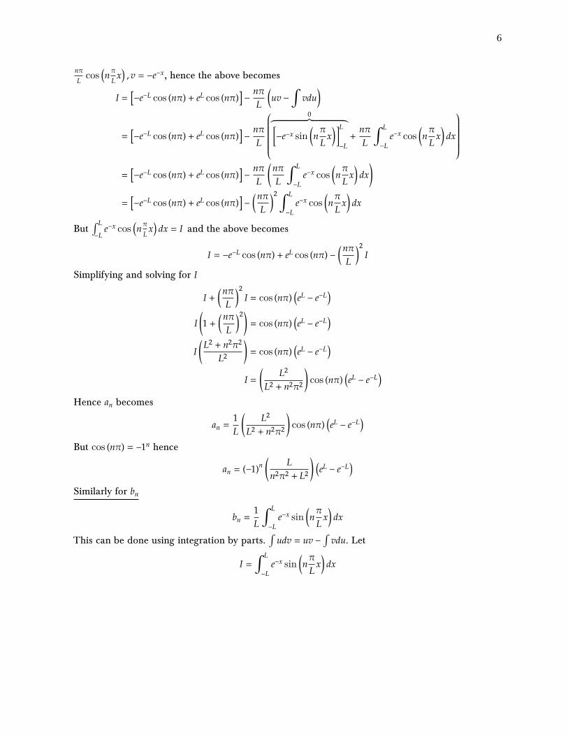
The following shows the approximation 𝑓 (𝑥) for increasing number of terms. Notice the Gibbsphenomena at the jump discontinuity.

-3 -2 -1 0 1 2 3

0.0

0.5

1.0

1.5

2.0

2.5

x

f(x)

Fourier series approximation, number of terms 3Showing 3 periods extenstion of -L..L, with L=1

-3 -2 -1 0 1 2 3

0.0

0.5

1.0

1.5

2.0

2.5

x

f(x)

Fourier series approximation, number of terms 10Showing 3 periods extenstion of -L..L, with L=1

9

-3 -2 -1 0 1 2 3

0.0

0.5

1.0

1.5

2.0

2.5

3.0

x

f(x)

Fourier series approximation, number of terms 50Showing 3 periods extenstion of -L..L, with L=1

1.2.2 Part d

The following is sketch of periodic extension of 𝑓 (𝑥) from 𝑥 = −𝐿⋯𝐿 (for 𝐿 = 1) for illustration. Thefunction will converge to 𝑓 (𝑥) between 𝑥 = −𝐿⋯𝐿 and between 𝑥 = −3𝐿⋯−𝐿 and between 𝑥 = 𝐿⋯3𝐿and so on. But at the jump discontinuities which occurs at 𝑥 = ⋯ ,−3𝐿, −𝐿, 𝐿, 3𝐿,⋯ it will converge tothe average 1

2 shown as small circles in the sketch.

oo o o

-3 -2 -1 1 2 3

0.20.40.60.81.0

Showing 3 periods extenstion of f(x) between -L..L, with L=1

By definitions,

𝑎0 =1𝑇 �

𝑇/2

−𝑇/2𝑓 (𝑥) 𝑑𝑥

𝑎𝑛 =1𝑇/2 �

𝑇/2

−𝑇/2𝑓 (𝑥) cos �𝑛 �

2𝜋𝑇 �

𝑥� 𝑑𝑥

𝑏𝑛 =1𝑇/2 �

𝑇/2

−𝑇/2𝑓 (𝑥) sin �𝑛 �

2𝜋𝑇 �

𝑥� 𝑑𝑥

The period here is 𝑇 = 2𝐿, therefore the above becomes

𝑎0 =12𝐿 �

𝐿

−𝐿𝑓 (𝑥) 𝑑𝑥

𝑎𝑛 =1𝐿 �

𝐿

−𝐿𝑓 (𝑥) cos �𝑛𝜋

𝐿𝑥� 𝑑𝑥

𝑏𝑛 =1𝐿 �

𝐿

−𝐿𝑓 (𝑥) sin �𝑛𝜋

𝐿𝑥� 𝑑𝑥

10

These are now evaluated for given 𝑓 (𝑥)

𝑎0 =12𝐿 �

𝐿

−𝐿𝑓 (𝑥) 𝑑𝑥

=12𝐿 ��

0

−𝐿𝑓 (𝑥) 𝑑𝑥 +�

𝐿

0𝑓 (𝑥) 𝑑𝑥�

=12𝐿 �

0 +�𝐿

0𝑥𝑑𝑥�

=12𝐿 �

𝑥2

2 �𝐿

0

=𝐿4

Now 𝑎𝑛 is found

𝑎𝑛 =1𝐿 �

𝐿

−𝐿𝑓 (𝑥) cos �𝑛𝜋

𝐿𝑥� 𝑑𝑥

=1𝐿 ��

0

−𝐿𝑓 (𝑥) cos �𝑛𝜋

𝐿𝑥� 𝑑𝑥 +�

𝐿

0𝑓 (𝑥) cos �𝑛𝜋

𝐿𝑥� 𝑑𝑥�

=1𝐿 �

𝐿

0𝑥 cos �𝑛𝜋

𝐿𝑥� 𝑑𝑥

Integration by parts. Let 𝑢 = 𝑥, 𝑑𝑢 = 1, 𝑑𝑣 = cos �𝑛𝜋𝐿 𝑥� , 𝑣 =

sin�𝑛𝜋𝐿 𝑥�

𝑛𝜋𝐿

, hence the above becomes

𝑎𝑛 =1𝐿

⎛⎜⎜⎜⎜⎜⎜⎜⎜⎜⎜⎝

0

��������������������������𝑛𝜋𝐿𝑥 sin �𝑛𝜋

𝐿𝑥��

𝐿

0−�

𝐿

0

sin �𝑛𝜋𝐿 𝑥�

𝑛𝜋𝐿

𝑑𝑥

⎞⎟⎟⎟⎟⎟⎟⎟⎟⎟⎟⎠

=1𝐿 �−𝐿𝑛𝜋 �

𝐿

0sin �𝑛𝜋

𝐿𝑥� 𝑑𝑥�

=1𝐿

⎛⎜⎜⎜⎜⎜⎜⎝−

𝐿𝑛𝜋

⎛⎜⎜⎜⎜⎜⎝− cos �𝑛𝜋

𝐿 𝑥�

𝑛𝜋𝐿

⎞⎟⎟⎟⎟⎟⎠

𝐿

0

⎞⎟⎟⎟⎟⎟⎟⎠

=1𝐿

⎛⎜⎜⎜⎜⎝�𝐿𝑛𝜋�

2

cos �𝑛𝜋𝐿𝑥�

𝐿

0

⎞⎟⎟⎟⎟⎠

=𝐿

𝑛2𝜋2 cos �𝑛𝜋𝐿𝑥�

𝐿

0

=𝐿

𝑛2𝜋2 �cos �𝑛𝜋𝐿𝐿� − 1�

=𝐿

𝑛2𝜋2 [−1𝑛 − 1]

11

Now 𝑏𝑛 is found

𝑏𝑛 =1𝐿 �

𝐿

−𝐿𝑓 (𝑥) sin �𝑛𝜋

𝐿𝑥� 𝑑𝑥

=1𝐿 ��

0

−𝐿𝑓 (𝑥) sin �𝑛𝜋

𝐿𝑥� 𝑑𝑥 +�

𝐿

0𝑓 (𝑥) sin �𝑛𝜋

𝐿𝑥� 𝑑𝑥�

=1𝐿 �

𝐿

0𝑥 sin �𝑛𝜋

𝐿𝑥� 𝑑𝑥

Integration by parts. Let 𝑢 = 𝑥, 𝑑𝑢 = 1, 𝑑𝑣 = sin �𝑛𝜋𝐿 𝑥� , 𝑣 =

− cos�𝑛𝜋𝐿 𝑥�

𝑛𝜋𝐿

, hence the above becomes

𝑏𝑛 =1𝐿

⎛⎜⎜⎜⎜⎜⎝�−

𝐿𝑛𝜋𝑥 cos �𝑛𝜋

𝐿𝑥��

𝐿

0+�

𝐿

0

cos �𝑛𝜋𝐿 𝑥�

𝑛𝜋𝐿

𝑑𝑥

⎞⎟⎟⎟⎟⎟⎠

=1𝐿 �−𝐿𝑛𝜋

�𝐿 cos �𝑛𝜋𝐿𝐿� − 0� +

𝐿𝑛𝜋 �

𝐿

0cos �𝑛𝜋

𝐿𝑥� 𝑑𝑥�

=1𝐿

⎛⎜⎜⎜⎜⎜⎜⎜⎜⎜⎜⎜⎜⎜⎜⎝

−𝐿2

𝑛𝜋(−1)𝑛 +

𝐿𝑛𝜋

0

�����������������⎡⎢⎢⎢⎢⎢⎣sin �𝑛𝜋

𝐿 𝑥�

𝑛𝜋𝐿

⎤⎥⎥⎥⎥⎥⎦

𝐿

0

⎞⎟⎟⎟⎟⎟⎟⎟⎟⎟⎟⎟⎟⎟⎟⎠

=𝐿𝑛𝜋

�− (−1)𝑛�

= (−1)𝑛+1𝐿𝑛𝜋

Summary

𝑎0 =𝐿4

𝑎𝑛 =𝐿

𝑛2𝜋2 [−1𝑛 − 1]

𝑏𝑛 = (−1)𝑛+1 𝐿

𝑛𝜋

𝑓 (𝑥) ≈ 𝑎0 +∞�𝑛=1

𝑎𝑛 cos �𝑛 �2𝜋𝑇 �

𝑥� + 𝑏𝑛 sin �𝑛 �2𝜋𝑇 �

𝑥�

≈ 𝑎0 +∞�𝑛=1

𝑎𝑛 cos �𝑛𝜋𝐿𝑥� + 𝑏𝑛 sin �𝑛𝜋

𝐿𝑥�

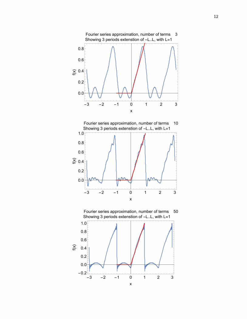
The following shows the approximation 𝑓 (𝑥) for increasing number of terms. Notice the Gibbsphenomena at the jump discontinuity.

12

-3 -2 -1 0 1 2 3

0.0

0.2

0.4

0.6

0.8

x

f(x)

Fourier series approximation, number of terms 3Showing 3 periods extenstion of -L..L, with L=1

-3 -2 -1 0 1 2 3

0.0

0.2

0.4

0.6

0.8

1.0

x

f(x)

Fourier series approximation, number of terms 10Showing 3 periods extenstion of -L..L, with L=1

-3 -2 -1 0 1 2 3-0.2

0.0

0.2

0.4

0.6

0.8

1.0

x

f(x)

Fourier series approximation, number of terms 50Showing 3 periods extenstion of -L..L, with L=1

13

1.3 Problem 3.2.4

96 Chapter 3. Fourier Series

3.2.3. Show that the Fourier series operation is linear: that is, show that theFourier series of c1 f (x) + c2g(x) is the sum of cl times the Fourier series off (x) and c2 times the Fourier series of g(x).

3.2.4. Suppose that f (x) is piecewise smooth. What value does the Fourier seriesof f (x) converge to at the endpoint x = -L? at x = L?

3.3 Fourier Cosine and Sine SeriesIn this section we show that the series of sines only (and the series of cosines only)are special cases of a Fourier series.

3.3.1 Fourier Sine SeriesOdd functions. An odd function is a function with the property f (-x)- f (x). The sketch of an odd function for x < 0 will be minus the mirror image off (x) for x > 0, as illustrated in Fig. 3.3.1. Examples of odd functions are f (x) = x3(in fact, any odd power) and f (x) = sin 4x. The integral of an odd function overa symmetric interval is zero (any contribution from x > 0 will be canceled by acontribution from x < 0).

Figure 3.3.1 An odd function.

Fourier series of odd functions. Let us calculate the Fourier coeffi-cients of an odd function:

ao1 fL

1 J_Lf (x) dx = 0

L

an = L ff(x)cosdx=0.L

Both are zero because the integrand, f (x) cos nirx/L, is odd (being the product ofan even function cos n7rx/L and an odd function f (x)). Since an = 0, all the cosinefunctions (which are even) will not appear in the Fourier series of an odd function.The Fourier series of an odd function is an infinite series of odd functions (sines):

00

f (x) - bn sinn1x,

(3.3.1)n=1

It will converge to the average value of the function at the end points after making periodic extensionsof the function. Specifically, at 𝑥 = −𝐿 the Fourier series will converge to

12�𝑓 (−𝐿) + 𝑓 (𝐿)�

And at 𝑥 = 𝐿 it will converge to

12�𝑓 (𝐿) + 𝑓 (−𝐿)�

Notice that if 𝑓 (𝐿) has same value as 𝑓 (−𝐿), then there will not be a jump discontinuity when periodicextension are made, and the above formula simply gives the value of the function at either end, sinceit is the same value.

1.4 Problem 3.3.2 (d)

114 Chapter 3. Fourier Series

(a)

(c)

f(x) = 1

f(x) _ {1 + x x > 0

(e) f(x) e-x x > 0

(b) f(x)=1+x

*(d) f(x) = ex

3.3.2. For the following functions, sketch the Fourier sine series of f (x) and deter-mine its Fourier coefficients.

(a) [Verify formula (3.3.13).]

(c) f(x)0

xx < L/2

x > L/2

1 x < L/6

(b) f (x) = 3 L/6 < x < L/20 x > L/2

* (d) f (x) 1 x < L/20 x > L/2

3.3.3. For the following functions, sketch the Fourier sine series of f (x). Also,roughly sketch the sum of a finite number of nonzero terms (at least thefirst two) of the Fourier sine series:

(a) f (x) = cos irx/L [Use formula (3.3.13).]

(b) f(x) _ { 1 x < L/20 x > L/2

(c) f (x) = x [Use formula (3.3.12).]

3.3.4. Sketch the Fourier cosine series of f (x) = sin irx/L. Briefly discuss.

3.3.5. For the following functions, sketch the Fourier cosine series of f (x) anddetermine its Fourier coefficients:

1 x < L/6(a) f (x) = x2 (b) f (x) = 3 L/6 < x < L/2 (c) f (x) =

0 x > L/2 fx x > L/2

3.3.6. For the following functions, sketch the Fourier cosine series of f (x). Also,roughly sketch the sum of a finite number of nonzero terms (at least thefirst two) of the Fourier cosine series:

(a) f (x) = x [Use formulas (3.3.22) and (3.3.23).]

(b) f (x) = 0 x<L/21 x > L12 [Use carefully formulas (3.2.6) and (3.2.7).]

_ 0 x < L/2(c) f (x)1 x > L/2 [Hint: Add the functions in parts (b) and (c).]

3.3.7. Show that ex is the sum of an even and an odd function.

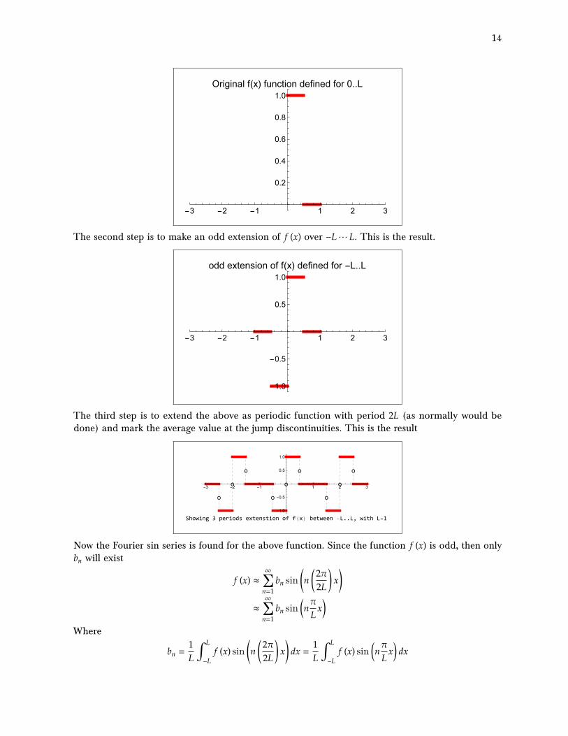
𝑓 (𝑥) =

⎧⎪⎪⎨⎪⎪⎩1 𝑥 < 𝐿

20 𝑥 > 𝐿

2

The first step is to sketch 𝑓 (𝑥) over 0⋯𝐿. This is the result for 𝐿 = 1 as an example.

14

-3 -2 -1 1 2 3

0.2

0.4

0.6

0.8

1.0

Original f(x) function defined for 0..L

The second step is to make an odd extension of 𝑓 (𝑥) over −𝐿⋯𝐿. This is the result.

-3 -2 -1 1 2 3

-1.0

-0.5

0.5

1.0

odd extension of f(x) defined for -L..L

The third step is to extend the above as periodic function with period 2𝐿 (as normally would bedone) and mark the average value at the jump discontinuities. This is the result

o

o o

o

o o

o

o

o

-3 -2 -1 1 2 3

-1.0

-0.5

0.5

1.0

Showing 3 periods extenstion of f(x) between -L..L, with L=1

Now the Fourier sin series is found for the above function. Since the function 𝑓 (𝑥) is odd, then only𝑏𝑛 will exist

𝑓 (𝑥) ≈∞�𝑛=1

𝑏𝑛 sin �𝑛 �2𝜋2𝐿 �

𝑥�

≈∞�𝑛=1

𝑏𝑛 sin �𝑛𝜋𝐿𝑥�

Where

𝑏𝑛 =1𝐿 �

𝐿

−𝐿𝑓 (𝑥) sin �𝑛 �

2𝜋2𝐿 �

𝑥� 𝑑𝑥 =1𝐿 �

𝐿

−𝐿𝑓 (𝑥) sin �𝑛𝜋

𝐿𝑥� 𝑑𝑥

15

Since 𝑓 (𝑥) sin �𝑛𝜋𝐿 𝑥� is even, then the above becomes

𝑏𝑛 =2𝐿 �

𝐿

0𝑓 (𝑥) sin �𝑛𝜋

𝐿𝑥� 𝑑𝑥

=2𝐿 ��

𝐿/2

01 × sin �𝑛𝜋

𝐿𝑥� 𝑑𝑥 +�

𝐿/2

00 × sin �𝑛𝜋

𝐿𝑥� 𝑑𝑥�

=2𝐿 �

𝐿/2

0sin �𝑛𝜋

𝐿𝑥� 𝑑𝑥

=2𝐿

⎡⎢⎢⎢⎢⎢⎣−

cos �𝑛𝜋𝐿 𝑥�

𝑛𝜋𝐿

⎤⎥⎥⎥⎥⎥⎦

𝐿/2

0

=−2𝑛𝜋 �

cos �𝑛𝜋𝐿𝑥��

𝐿/2

0

=−2𝑛𝜋 �

cos �𝑛𝜋𝐿𝐿2�− 1�

=−2𝑛𝜋 �

cos �𝑛𝜋2� − 1�

=2𝑛𝜋 �

1 − cos �𝑛𝜋2��

Therefore

𝑓 (𝑥) ≈∞�𝑛=1

2𝑛𝜋

�1 − cos �𝑛𝜋2�� sin �𝑛𝜋

𝐿𝑥�

The following shows the approximation 𝑓 (𝑥) for increasing number of terms. Notice the Gibbsphenomena at the jump discontinuity.

-1.0 -0.5 0.0 0.5 1.0

-1.0

-0.5

0.0

0.5

1.0

x

f(x)

Fourier series approximation, number of terms 3Showing 3 periods extenstion of -L..L, with L=1

16

-1.0 -0.5 0.0 0.5 1.0

-1.0

-0.5

0.0

0.5

1.0

x

f(x)

Fourier series approximation, number of terms 10Showing 3 periods extenstion of -L..L, with L=1

-1.0 -0.5 0.0 0.5 1.0

-1.0

-0.5

0.0

0.5

1.0

x

f(x)

Fourier series approximation, number of terms 50Showing 3 periods extenstion of -L..L, with L=1

1.5 Problem 3.3.3 (b)

114 Chapter 3. Fourier Series

(a)

(c)

f(x) = 1

f(x) _ {1 + x x > 0

(e) f(x) e-x x > 0

(b) f(x)=1+x

*(d) f(x) = ex

3.3.2. For the following functions, sketch the Fourier sine series of f (x) and deter-mine its Fourier coefficients.

(a) [Verify formula (3.3.13).]

(c) f(x)0

xx < L/2

x > L/2

1 x < L/6

(b) f (x) = 3 L/6 < x < L/20 x > L/2

* (d) f (x) 1 x < L/20 x > L/2

3.3.3. For the following functions, sketch the Fourier sine series of f (x). Also,roughly sketch the sum of a finite number of nonzero terms (at least thefirst two) of the Fourier sine series:

(a) f (x) = cos irx/L [Use formula (3.3.13).]

(b) f(x) _ { 1 x < L/20 x > L/2

(c) f (x) = x [Use formula (3.3.12).]

3.3.4. Sketch the Fourier cosine series of f (x) = sin irx/L. Briefly discuss.

3.3.5. For the following functions, sketch the Fourier cosine series of f (x) anddetermine its Fourier coefficients:

1 x < L/6(a) f (x) = x2 (b) f (x) = 3 L/6 < x < L/2 (c) f (x) =

0 x > L/2 fx x > L/2

3.3.6. For the following functions, sketch the Fourier cosine series of f (x). Also,roughly sketch the sum of a finite number of nonzero terms (at least thefirst two) of the Fourier cosine series:

(a) f (x) = x [Use formulas (3.3.22) and (3.3.23).]

(b) f (x) = 0 x<L/21 x > L12 [Use carefully formulas (3.2.6) and (3.2.7).]

_ 0 x < L/2(c) f (x)1 x > L/2 [Hint: Add the functions in parts (b) and (c).]

3.3.7. Show that ex is the sum of an even and an odd function.

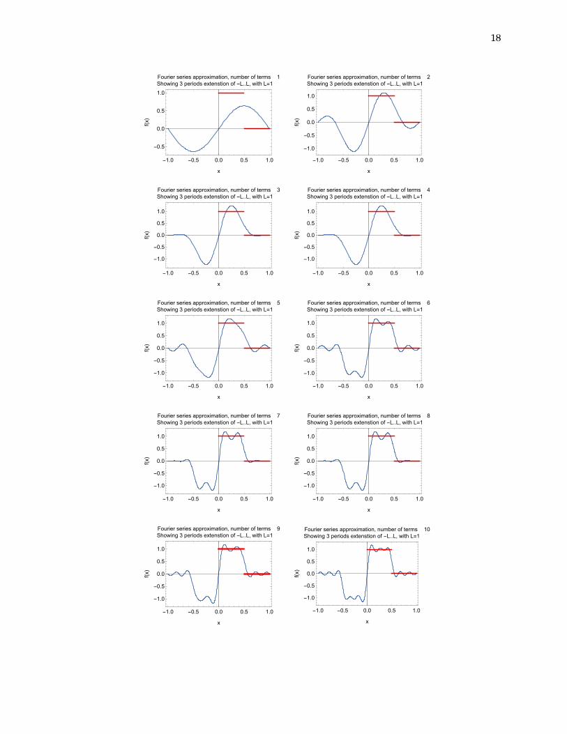
This is the same problem as 3.3.2 part (d). But it asks to plot for 𝑛 = 1 and 𝑛 = 2 in the sum. Thesketch of the Fourier sin series was done above in solving 3.3.2 part(d) and will not be repeated

17

again. From above, it was found that

𝑓 (𝑥) ≈∞�𝑛=1

𝐵𝑛 sin �𝑛𝜋𝐿𝑥�

Where 𝐵𝑛 =2𝑛𝜋�1 − cos �𝑛𝜋2 ��. The following is the plot for 𝑛 = 1⋯10.

18

-1.0 -0.5 0.0 0.5 1.0

-0.5

0.0

0.5

1.0

x

f(x)

Fourier series approximation, number of terms 1Showing 3 periods extenstion of -L..L, with L=1

-1.0 -0.5 0.0 0.5 1.0

-1.0

-0.5

0.0

0.5

1.0

x

f(x)

Fourier series approximation, number of terms 2Showing 3 periods extenstion of -L..L, with L=1

-1.0 -0.5 0.0 0.5 1.0

-1.0

-0.5

0.0

0.5

1.0

x

f(x)

Fourier series approximation, number of terms 3Showing 3 periods extenstion of -L..L, with L=1

-1.0 -0.5 0.0 0.5 1.0

-1.0

-0.5

0.0

0.5

1.0

x

f(x)

Fourier series approximation, number of terms 4Showing 3 periods extenstion of -L..L, with L=1

-1.0 -0.5 0.0 0.5 1.0

-1.0

-0.5

0.0

0.5

1.0

x

f(x)

Fourier series approximation, number of terms 5Showing 3 periods extenstion of -L..L, with L=1

-1.0 -0.5 0.0 0.5 1.0

-1.0

-0.5

0.0

0.5

1.0

x

f(x)

Fourier series approximation, number of terms 6Showing 3 periods extenstion of -L..L, with L=1

-1.0 -0.5 0.0 0.5 1.0

-1.0

-0.5

0.0

0.5

1.0

x

f(x)

Fourier series approximation, number of terms 7Showing 3 periods extenstion of -L..L, with L=1

-1.0 -0.5 0.0 0.5 1.0

-1.0

-0.5

0.0

0.5

1.0

x

f(x)

Fourier series approximation, number of terms 8Showing 3 periods extenstion of -L..L, with L=1

-1.0 -0.5 0.0 0.5 1.0

-1.0

-0.5

0.0

0.5

1.0

x

f(x)

Fourier series approximation, number of terms 9Showing 3 periods extenstion of -L..L, with L=1

-1.0 -0.5 0.0 0.5 1.0

-1.0

-0.5

0.0

0.5

1.0

x

f(x)

Fourier series approximation, number of terms 10Showing 3 periods extenstion of -L..L, with L=1

19

1.6 Problem 3.3.8

3.3. Cosine and Sine Series 115

3.3.8. (a) Determine formulas for the even extension of any f (x). Compare tothe formula for the even part of f (x).

(b) Do the same for the odd extension of f (x) and the odd part of f (x).

(c) Calculate and sketch the four functions of parts (a) and (b) if

= J x x>0f(x x2 x <0.

Graphically add the even and odd parts of f (x). What occurs? Simi-larly, add the even and odd extensions. What occurs then?

3.3.9. What is the sum of the Fourier sine series of f (x) and the Fourier cosineseries of f (x)? [What is the sum of the even and odd extensions of f (x)?]

2

*3.3.10. If f (x) = e_z x > 0 , what are the even and odd parts of f (x)?

3.3.11. Given a sketch of f(x), describe a procedure to sketch the even and odd

parts of f (x).

3.3.12. (a) Graphically show that the even terms (n even) of the Fourier sine seriesof any function on 0 < x < L are odd .(antisymmetric) around x = L/2.

(b) Consider a function f (x) that is odd around x = L/2. Show that theodd coefficients (n odd) of the Fourier sine series of f (x) on 0 < x < Lare zero.

*3.3.13. Consider a function f (x) that is even around x = L/2. Show that the evencoefficients (n even) of the Fourier sine series of f (x) on 0 < x < L are zero.

3.3.14. (a) Consider a function f (x) that is even around x = L/2. Show thatthe odd coefficients (n odd) of the Fourier cosine series of f (x) on0 < x < L are zero.

(b) Explain the result of part (a) by considering a Fourier cosine series off (x) on the interval 0 < x < L/2.

3.3.15. Consider a function f (x) that is odd around x = L/2. Show that the evencoefficients (n even) of the Fourier cosine series of f (x) on 0 < x < L arezero.

3.3.16. Fourier series can be defined on other intervals besides -L < x < L. Sup-pose that g(y) is defined for a < y < b. Represent g(y) using periodictrigonometric functions with period b - a. Determine formulas for the coef-ficients. [Hint: Use the linear transformation

a+b b-a2 + 2L

1.6.1 Part (a)

The even extension of 𝑓 (𝑥) is⎧⎪⎪⎨⎪⎪⎩

𝑓 (𝑥) 𝑥 > 0𝑓 (−𝑥) 𝑥 < 0

But the even part of 𝑓 (𝑥) is12�𝑓 (𝑥) + 𝑓 (−𝑥)�

1.6.2 Part (b)

The odd extension of 𝑓 (𝑥) is⎧⎪⎪⎨⎪⎪⎩

𝑓 (𝑥) 𝑥 > 0−𝑓 (−𝑥) 𝑥 < 0

While the odd part of 𝑓 (𝑥) is12�𝑓 (𝑥) − 𝑓 (−𝑥)�

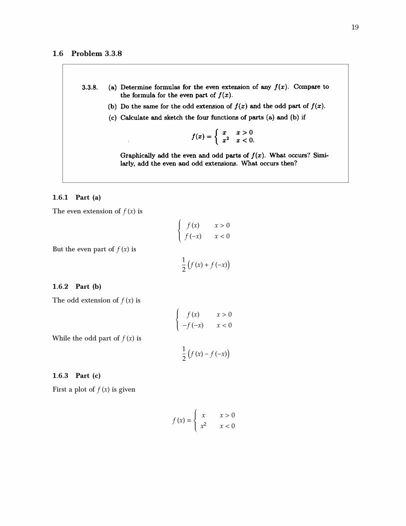
1.6.3 Part (c)

First a plot of 𝑓 (𝑥) is given

𝑓 (𝑥) =

⎧⎪⎪⎨⎪⎪⎩𝑥 𝑥 > 0𝑥2 𝑥 < 0

20

-1.0 -0.5 0.0 0.5 1.00.0

0.2

0.4

0.6

0.8

1.0

x

f(x)

Plot of f(x)

A plot of even extension and the even part for 𝑓 (𝑥) Is given below

-1.0 -0.5 0.0 0.5 1.0

0.0

0.2

0.4

0.6

0.8

1.0

x

f(x)

Plot of even extension

-1.0 -0.5 0.0 0.5 1.0

0.0

0.2

0.4

0.6

0.8

1.0

x

f(x)

Plot of even part

A plot of odd extension and the odd part is given below

-1.0 -0.5 0.0 0.5 1.0

-1.0

-0.5

0.0

0.5

1.0

x

function

Plot of odd extension

-1.0 -0.5 0.0 0.5 1.0

-0.10

-0.05

0.00

0.05

0.10

x

function

Plot of odd part of f(x)

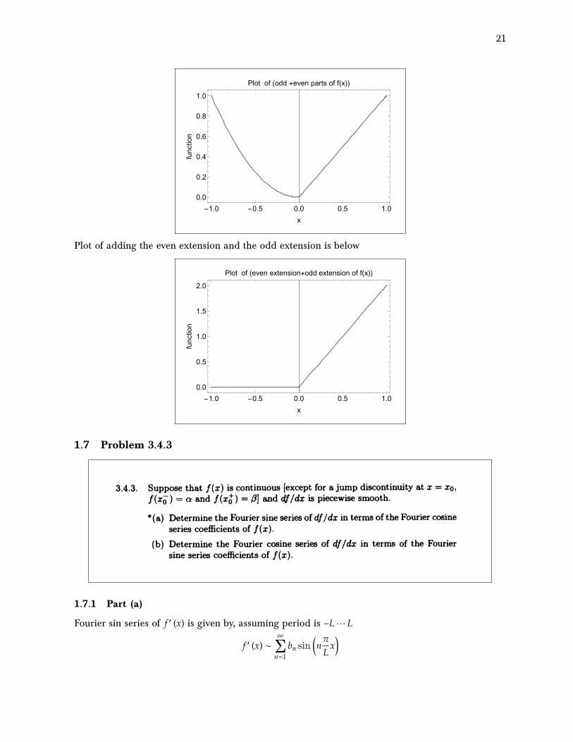
Adding the even part and the odd part gives back the original function

21

-1.0 -0.5 0.0 0.5 1.0

0.0

0.2

0.4

0.6

0.8

1.0

x

function

Plot of (odd +even parts of f(x))

Plot of adding the even extension and the odd extension is below

-1.0 -0.5 0.0 0.5 1.0

0.0

0.5

1.0

1.5

2.0

x

function

Plot of (even extension+odd extension of f(x))

1.7 Problem 3.4.3

3.4. Term-by-Term Differentiation 125

3.4.3. Suppose that f (x) is continuous [except for a jump discontinuity at x = x°if (xa) = a and f (xo) = 01 and df /dx is piecewise smooth.

*(a) Determine the Fourier sine series of df /dx in terms of the Fourier cosineseries coefficients of f (x).

(b) Determine the Fourier cosine series of df /dx in terms of the Fouriersine series coefficients of f(x).

3.4.4. Suppose that f (x) and df /dx are piecewise smooth.

(a) Prove that the Fourier sine series of a continuous function f (x) canonly be differentiated term by term if f (0) = 0 and f (L) = 0.

(b) Prove that the Fourier cosine series of a continuous function f (x) canbe differentiated term by term.

3.4.5. Using (3.3.13) determine the Fourier cosine series of sin 7rx/L.

3.4.6. There are some things wrong in the following demonstration. Find themistakes and correct them.

In this exercise we attempt to obtain the Fourier cosine coefficients of ex:

00 nirxex=A°+E A.cos r .

n=1

Differentiating yields

00 nir nirxe2=-L ,

n=1

the Fourier sine series of ex. Differentiating again yields

(3.4.22)

°O 2n7rex - ( L) An cos nLx (3.4.23)

n=1

Since equations (3.4.22) and (3.4.23) give the Fourier cosine series of ex,

they must be identical. Thus,

`40 0 (obviously wrong!).An =0

By correcting the mistakes, you should be able to obtain A° and An withoutusing the typical technique, that is, An = 2/L f L ex cos nirx/L dx.

3.4.7. Prove that the Fourier series of a continuous function u(x, t) can be differ-entiated term by term with respect to the parameter t if 8u/8t is piecewisesmooth.

1.7.1 Part (a)

Fourier sin series of 𝑓′ (𝑥) is given by, assuming period is −𝐿⋯𝐿

𝑓′ (𝑥) ∼∞�𝑛=1

𝑏𝑛 sin �𝑛𝜋𝐿𝑥�

22

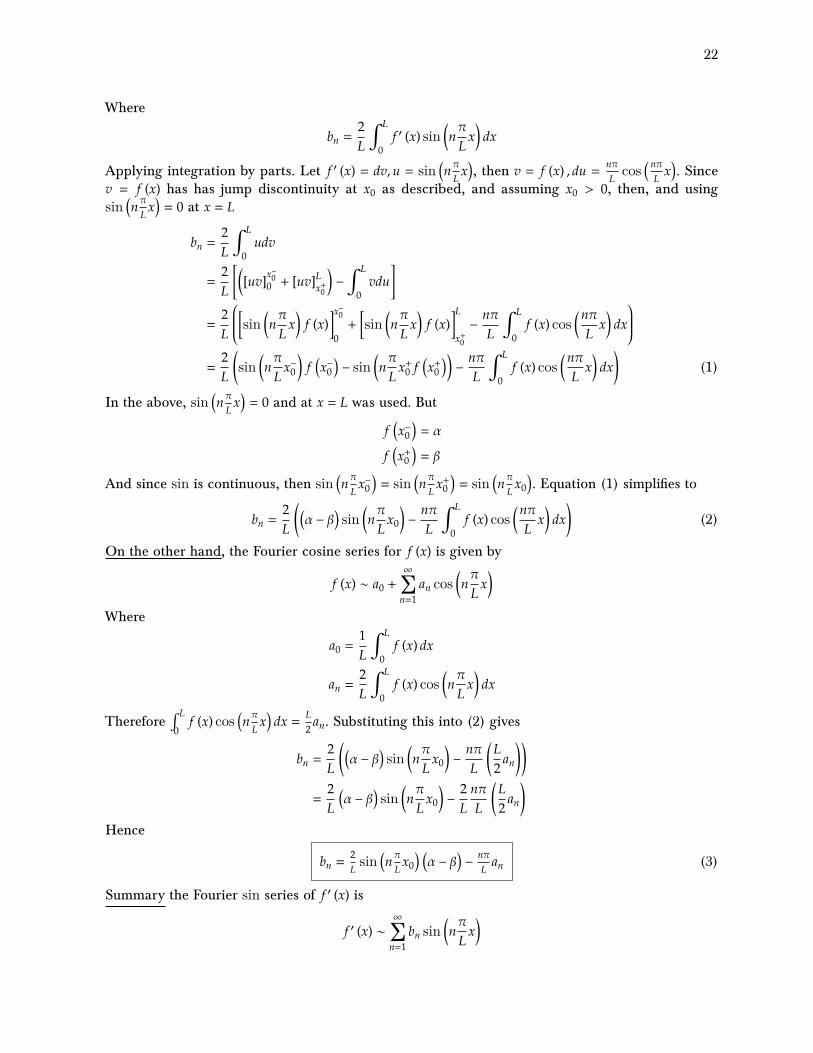
Where

𝑏𝑛 =2𝐿 �

𝐿

0𝑓′ (𝑥) sin �𝑛𝜋

𝐿𝑥� 𝑑𝑥

Applying integration by parts. Let 𝑓′ (𝑥) = 𝑑𝑣, 𝑢 = sin �𝑛𝜋𝐿 𝑥�, then 𝑣 = 𝑓 (𝑥) , 𝑑𝑢 = 𝑛𝜋

𝐿 cos �𝑛𝜋𝐿 𝑥�. Since𝑣 = 𝑓 (𝑥) has has jump discontinuity at 𝑥0 as described, and assuming 𝑥0 > 0, then, and usingsin �𝑛𝜋

𝐿 𝑥� = 0 at 𝑥 = 𝐿

𝑏𝑛 =2𝐿 �

𝐿

0𝑢𝑑𝑣

=2𝐿 ��[𝑢𝑣]𝑥

−00 + [𝑢𝑣]𝐿𝑥+0 � −�

𝐿

0𝑣𝑑𝑢�

=2𝐿

⎛⎜⎜⎜⎜⎝�sin �𝑛

𝜋𝐿𝑥� 𝑓 (𝑥)�

𝑥−0

0+ �sin �𝑛

𝜋𝐿𝑥� 𝑓 (𝑥)�

𝐿

𝑥+0−𝑛𝜋𝐿 �

𝐿

0𝑓 (𝑥) cos �𝑛𝜋

𝐿𝑥� 𝑑𝑥

⎞⎟⎟⎟⎟⎠

=2𝐿 �

sin �𝑛𝜋𝐿𝑥−0� 𝑓 �𝑥−0� − sin �𝑛𝜋

𝐿𝑥+0𝑓 �𝑥+0 �� −

𝑛𝜋𝐿 �

𝐿

0𝑓 (𝑥) cos �𝑛𝜋

𝐿𝑥� 𝑑𝑥� (1)

In the above, sin �𝑛𝜋𝐿 𝑥� = 0 and at 𝑥 = 𝐿 was used. But

𝑓 �𝑥−0� = 𝛼

𝑓 �𝑥+0 � = 𝛽

And since sin is continuous, then sin �𝑛𝜋𝐿 𝑥

−0� = sin �𝑛𝜋

𝐿 𝑥+0 � = sin �𝑛𝜋

𝐿 𝑥0�. Equation (1) simplifies to

𝑏𝑛 =2𝐿 ��𝛼 − 𝛽� sin �𝑛𝜋

𝐿𝑥0� −

𝑛𝜋𝐿 �

𝐿

0𝑓 (𝑥) cos �𝑛𝜋

𝐿𝑥� 𝑑𝑥� (2)

On the other hand, the Fourier cosine series for 𝑓 (𝑥) is given by

𝑓 (𝑥) ∼ 𝑎0 +∞�𝑛=1

𝑎𝑛 cos �𝑛𝜋𝐿𝑥�

Where

𝑎0 =1𝐿 �

𝐿

0𝑓 (𝑥) 𝑑𝑥

𝑎𝑛 =2𝐿 �

𝐿

0𝑓 (𝑥) cos �𝑛𝜋

𝐿𝑥� 𝑑𝑥

Therefore ∫𝐿

0𝑓 (𝑥) cos �𝑛𝜋

𝐿 𝑥� 𝑑𝑥 =𝐿2𝑎𝑛. Substituting this into (2) gives

𝑏𝑛 =2𝐿 ��𝛼 − 𝛽� sin �𝑛𝜋

𝐿𝑥0� −

𝑛𝜋𝐿 �

𝐿2𝑎𝑛��

=2𝐿�𝛼 − 𝛽� sin �𝑛𝜋

𝐿𝑥0� −

2𝐿𝑛𝜋𝐿 �

𝐿2𝑎𝑛�

Hence

𝑏𝑛 =2𝐿 sin �𝑛𝜋

𝐿 𝑥0� �𝛼 − 𝛽� −𝑛𝜋𝐿 𝑎𝑛 (3)

Summary the Fourier sin series of 𝑓′ (𝑥) is

𝑓′ (𝑥) ∼∞�𝑛=1

𝑏𝑛 sin �𝑛𝜋𝐿𝑥�

23

With 𝑏𝑛 given by (3). The above is in terms of 𝑎𝑛, which is the Fourier cosine series of 𝑓 (𝑥), which iswhat required to show. In addition, the cos series of 𝑓 (𝑥) can also be written in terms of sin series of𝑓′ (𝑥). From (3), solving for 𝑎𝑛

𝑎𝑛 =𝐿𝑛𝜋𝑏𝑛 −

2𝑛𝜋

sin �𝑛𝜋𝐿𝑥0� �𝛼 − 𝛽�

𝑓 (𝑥) ∼ 𝑎0 +∞�𝑛=1

1𝑛 �

𝐿𝜋𝑏𝑛 −

2𝜋

sin �𝑛𝜋𝐿𝑥0� �𝛼 − 𝛽�� cos �𝑛𝜋

𝐿𝑥�

This shows more clearly that the Fourier series of 𝑓 (𝑥) has order of convergence in 𝑎𝑛 as1𝑛 as expected.

1.7.2 Part (b)

Fourier cos series of 𝑓′ (𝑥) is given by, assuming period is −𝐿⋯𝐿

𝑓′ (𝑥) ∼∞�𝑛=0

𝑎𝑛 cos �𝑛𝜋𝐿𝑥�

Where

𝑎0 =1𝐿 �

𝐿

0𝑓′ (𝑥) 𝑑𝑥

=1𝐿

⎛⎜⎜⎜⎝�

𝑥−0

0𝑓′ (𝑥) 𝑑𝑥 +�

𝐿

𝑥+0𝑓′ (𝑥) 𝑑𝑥

⎞⎟⎟⎟⎠

=1𝐿 ��𝑓 (𝑥)�

𝑥−00+ �𝑓 (𝑥)�

𝐿

𝑥+0�

=1𝐿��𝛼 − 𝑓 (0)� + �𝑓 (𝐿) − 𝛽��

=�𝛼 − 𝛽�𝐿

+𝑓 (0) + 𝑓 (𝐿)

𝐿And for 𝑛 > 0

𝑎𝑛 =2𝐿 �

𝐿

0𝑓′ (𝑥) cos �𝑛𝜋

𝐿𝑥� 𝑑𝑥

Applying integration by parts. Let 𝑓′ (𝑥) = 𝑑𝑣, 𝑢 = cos �𝑛𝜋𝐿 𝑥�, then 𝑣 = 𝑓 (𝑥) , 𝑑𝑢 =

−𝑛𝜋𝐿 sin �𝑛𝜋𝐿 𝑥�. Since

𝑣 = 𝑓 (𝑥) has has jump discontinuity at 𝑥0 as described, then

𝑎𝑛 =2𝐿 �

𝐿

0𝑢𝑑𝑣

=2𝐿 ��[𝑢𝑣]𝑥

−00 + [𝑢𝑣]𝐿𝑥+0 � −�

𝐿

0𝑣𝑑𝑢�

=2𝐿

⎛⎜⎜⎜⎜⎝�cos �𝑛𝜋

𝐿𝑥� 𝑓 (𝑥)�

𝑥−0

0+ �cos �𝑛𝜋

𝐿𝑥� 𝑓 (𝑥)�

𝐿

𝑥+0+𝑛𝜋𝐿 �

𝐿

0𝑓 (𝑥) sin �𝑛𝜋

𝐿𝑥� 𝑑𝑥

⎞⎟⎟⎟⎟⎠

=2𝐿 �

cos �𝑛𝜋𝐿𝑥−0� 𝑓 �𝑥−0� − 𝑓 (0) + cos (𝑛𝜋) 𝑓 (𝐿) − cos �𝑛𝜋

𝐿𝑥+0 � 𝑓 �𝑥+0 � +

𝑛𝜋𝐿 �

𝐿

0𝑓 (𝑥) sin �𝑛𝜋

𝐿𝑥� 𝑑𝑥� (1)

But

𝑓 �𝑥−0� = 𝛼

𝑓 �𝑥+0 � = 𝛽

24

And since cos is continuous, then cos �𝑛𝜋𝐿 𝑥

−0� = cos �𝑛𝜋

𝐿 𝑥+0 � = cos �𝑛𝜋

𝐿 𝑥0�, therefore (1) becomes

𝑎𝑛 =2𝐿 �

cos (𝑛𝜋) 𝑓 (𝐿) − 𝑓 (0) + cos �𝑛𝜋𝐿𝑥0� �𝛼 − 𝛽� +

𝑛𝜋𝐿 �

𝐿

0𝑓 (𝑥) sin �𝑛𝜋

𝐿𝑥� 𝑑𝑥� (2)

On the other hand, the Fourier 𝑠𝑖𝑛 series for 𝑓 (𝑥) is given by

𝑓 (𝑥) ∼∞�𝑛=0

𝑏𝑛 sin �𝑛𝜋𝐿𝑥�

Where

𝑏𝑛 =2𝐿 �

𝐿

0𝑓 (𝑥) sin �𝑛𝜋

𝐿𝑥� 𝑑𝑥

Therefore ∫𝐿

0𝑓 (𝑥) sin �𝑛𝜋

𝐿 𝑥� 𝑑𝑥 =𝐿2𝑏𝑛. Substituting this into (2) gives

𝑎𝑛 =2𝐿 �

cos (𝑛𝜋) 𝑓 (𝐿) − 𝑓 (0) + cos �𝑛𝜋𝐿𝑥0� �𝛼 − 𝛽� +

𝑛𝜋𝐿𝐿2𝑏𝑛�

=2𝐿

cos (𝑛𝜋) 𝑓 (𝐿) − 2𝐿𝑓 (0) +

2𝐿

cos �𝑛𝜋𝐿𝑥0� �𝛼 − 𝛽� +

2𝐿𝑛𝜋2𝑏𝑛

=2𝐿�(−1𝑛) 𝑓 (𝐿) − 𝑓 (0)� +

2𝐿

cos �𝑛𝜋𝐿𝑥0� �𝛼 − 𝛽� +

𝑛𝜋𝐿𝑏𝑛

Hence

𝑎𝑛 =2𝐿�(−1𝑛) 𝑓 (𝐿) − 𝑓 (0)� + 2

𝐿 cos �𝑛𝜋𝐿 𝑥0� �𝛼 − 𝛽� +

𝑛𝜋𝐿 𝑏𝑛 (3)

Summary the Fourier cos series of 𝑓′ (𝑥) is

𝑓′ (𝑥) ∼∞�𝑛=0

𝑎𝑛 cos �𝑛𝜋𝐿𝑥�

𝑎0 =�𝛼 − 𝛽�𝐿

+𝑓 (0) + 𝑓 (𝐿)

𝐿

𝑎𝑛 =2𝐿�(−1𝑛) 𝑓 (𝐿) − 𝑓 (0)� +

2𝐿

cos �𝑛𝜋𝐿𝑥0� �𝛼 − 𝛽� +

𝑛𝜋𝐿𝑏𝑛

The above is in terms of 𝑏𝑛, which is the Fourier 𝑠𝑖𝑛 series of 𝑓 (𝑥), which is what required to show.

25

1.8 Problem 3.4.9

126 Chapter 3. Fourier Series

3.4.8. Considerau _ a2uat kaxe

subject to

au/ax(0,t) = 0, au/ax(L,t) = 0, and u(x,0) = f(x).

Solve in the following way. Look for the solution as a Fourier cosine se-ries. Assume that u and au/ax are continuous and a2u/axe and au/at arepiecewise smooth. Justify all differentiations of infinite series.

*3.4.9 Consider the heat equation with a known source q(x, t):

2

= k jx2 + q(x, t) with u(0, t) = 0 and u(L, t) = 0.

Assume that q(x, t) (for each t > 0) is a piecewise smooth function of x.Also assume that u and au/ax are continuous functions of x (for t > 0) anda2u/axe and au/at are piecewise smooth. Thus,

u(x, t) _ N,(t) sin .Lx.n=1

What ordinary differential equation does satisfy? Do not solve thisdifferential equation.

3.4.10. Modify Exercise 3.4.9 if instead au/ax(0, t) = 0 and au/ax(L, t) = 0.

3.4.11. Consider the nonhomogeneous heat equation (with a steady heat source):

2

at kax2 +g(x).

Solve this equation with the initial condition

u(x,0) = f(x)

and the boundary conditions

u(O,t) = 0 and u(L, t) = 0.

Assume that a continuous solution exists (with continuous derivatives).[Hints: Expand the solution as a Fourier sine series (i.e., use the methodof eigenfunction expansion). Expand g(x) as a Fourier sine series. Solvefor the Fourier sine series of the solution. Justify all differentiations withrespect to x.]

*3.4.12. Solve the following nonhomogeneous problem:

2

= k5-2 + e-t + e- 2tcos 3Lx [assume that 2 # k(37r/L)2]

The PDE is𝜕𝑢𝜕𝑡

= 𝑘𝜕2𝑢𝜕𝑥2

+ 𝑞 (𝑥, 𝑡) (1)

Since the boundary conditions are homogenous Dirichlet conditions, then the solution can be writtendown as

𝑢 (𝑥, 𝑡) =∞�𝑛=1

𝑏𝑛 (𝑡) sin �𝑛𝜋𝐿𝑥�

Since the solution is assumed to be continuous with continuous derivative, then term by termdi�erentiation is allowed w.r.t. 𝑥

𝜕𝑢𝜕𝑥

=∞�𝑛=1

𝑛𝜋𝐿𝑏𝑛 (𝑡) cos �𝑛𝜋

𝐿𝑥�

𝜕2𝑢𝜕𝑥2

= −∞�𝑛=1

�𝑛𝜋𝐿�2𝑏𝑛 (𝑡) sin �𝑛

𝜋𝐿𝑥� (2)

Also using assumption that 𝜕𝑢𝜕𝑡 is smooth, then

𝜕𝑢𝜕𝑡

=∞�𝑛=1

𝑑𝑏𝑛 (𝑡)𝑑𝑡

sin �𝑛𝜋𝐿𝑥� (3)

Substituting (2,3) into (1) gives∞�𝑛=1

𝑑𝑏𝑛 (𝑡)𝑑𝑡

sin �𝑛𝜋𝐿𝑥� = −𝑘

∞�𝑛=1

�𝑛𝜋𝐿�2𝑏𝑛 (𝑡) sin �𝑛

𝜋𝐿𝑥� + 𝑞 (𝑥, 𝑡) (4)

Expanding 𝑞 (𝑥, 𝑡) as Fourier sin series in 𝑥. Hence

𝑞 (𝑥, 𝑡) =∞�𝑛=1

𝑞𝑛 (𝑡) sin �𝑛𝜋𝐿𝑥�

Where now 𝑞𝑛 (𝑡) are time dependent given by (by orthogonality)

𝑞𝑛 (𝑡) =2𝐿 �

𝐿

0𝑞 (𝑥, 𝑡) sin �𝑛𝜋

𝐿𝑥�

26

Hence (4) becomes∞�𝑛=1

𝑑𝑏𝑛 (𝑡)𝑑𝑡

sin �𝑛𝜋𝐿𝑥� = −

∞�𝑛=1

𝑘 �𝑛𝜋𝐿�2𝑏𝑛 (𝑡) sin �𝑛

𝜋𝐿𝑥� +

∞�𝑛=1

𝑞 (𝑡)𝑛 sin �𝑛𝜋𝐿𝑥�

Applying orthogonality the above reduces to one term only

𝑑𝑏𝑛 (𝑡)𝑑𝑡

sin �𝑛𝜋𝐿𝑥� = −𝑘 �

𝑛𝜋𝐿�2𝑏𝑛 (𝑡) sin �𝑛

𝜋𝐿𝑥� + 𝑞 (𝑡)𝑛 sin �𝑛𝜋

𝐿𝑥�

Dividing by sin �𝑛𝜋𝐿 𝑥� ≠ 0

𝑑𝑏𝑛 (𝑡)𝑑𝑡

= −𝑘 �𝑛𝜋𝐿�2𝑏𝑛 (𝑡) + 𝑞𝑛 (𝑡)

𝑑𝑏𝑛 (𝑡)𝑑𝑡

+ 𝑘 �𝑛𝜋𝐿�2𝐵𝑛 (𝑡) = 𝑞𝑛 (𝑡) (5)

The above is the ODE that needs to be solved for 𝑏𝑛 (𝑡). It is first order inhomogeneous ODE. Thequestion asks to stop here.

1.9 Problem 3.4.11

126 Chapter 3. Fourier Series

3.4.8. Considerau _ a2uat kaxe

subject to

au/ax(0,t) = 0, au/ax(L,t) = 0, and u(x,0) = f(x).

Solve in the following way. Look for the solution as a Fourier cosine se-ries. Assume that u and au/ax are continuous and a2u/axe and au/at arepiecewise smooth. Justify all differentiations of infinite series.

*3.4.9 Consider the heat equation with a known source q(x, t):

2

= k jx2 + q(x, t) with u(0, t) = 0 and u(L, t) = 0.

Assume that q(x, t) (for each t > 0) is a piecewise smooth function of x.Also assume that u and au/ax are continuous functions of x (for t > 0) anda2u/axe and au/at are piecewise smooth. Thus,

u(x, t) _ N,(t) sin .Lx.n=1

What ordinary differential equation does satisfy? Do not solve thisdifferential equation.

3.4.10. Modify Exercise 3.4.9 if instead au/ax(0, t) = 0 and au/ax(L, t) = 0.

3.4.11. Consider the nonhomogeneous heat equation (with a steady heat source):

2

at kax2 +g(x).

Solve this equation with the initial condition

u(x,0) = f(x)

and the boundary conditions

u(O,t) = 0 and u(L, t) = 0.

Assume that a continuous solution exists (with continuous derivatives).[Hints: Expand the solution as a Fourier sine series (i.e., use the methodof eigenfunction expansion). Expand g(x) as a Fourier sine series. Solvefor the Fourier sine series of the solution. Justify all differentiations withrespect to x.]

*3.4.12. Solve the following nonhomogeneous problem:

2

= k5-2 + e-t + e- 2tcos 3Lx [assume that 2 # k(37r/L)2]The PDE is

𝜕𝑢𝜕𝑡

= 𝑘𝜕2𝑢𝜕𝑥2

+ 𝑔 (𝑥) (1)

Since the boundary conditions are homogenous Dirichlet conditions, then the solution can be writtendown as

𝑢 (𝑥, 𝑡) =∞�𝑛=1

𝑏𝑛 (𝑡) sin �𝑛𝜋𝐿𝑥�

Since the solution is assumed to be continuous with continuous derivative, then term by term

27

di�erentiation is allowed w.r.t. 𝑥𝜕𝑢𝜕𝑥

=∞�𝑛=1

𝑛𝜋𝐿𝑏𝑛 (𝑡) cos �𝑛𝜋

𝐿𝑥�

𝜕2𝑢𝜕𝑥2

= −∞�𝑛=1

�𝑛𝜋𝐿�2𝑏𝑛 (𝑡) sin �𝑛

𝜋𝐿𝑥� (2)

Also using assumption that 𝜕𝑢𝜕𝑡 is smooth, then

𝜕𝑢𝜕𝑡

=∞�𝑛=1

𝑑𝑏𝑛 (𝑡)𝑑𝑡

sin �𝑛𝜋𝐿𝑥� (3)

Substituting (2,3) into (1) gives∞�𝑛=1

𝑑𝑏𝑛 (𝑡)𝑑𝑡

sin �𝑛𝜋𝐿𝑥� = −𝑘

∞�𝑛=1

�𝑛𝜋𝐿�2𝑏𝑛 (𝑡) sin �𝑛

𝜋𝐿𝑥� + 𝑔 (𝑥) (4)

Using hint given in the problem, which is to expand 𝑔 (𝑥) as Fourier sin series. Hence

𝑔 (𝑥) =∞�𝑛=1

𝑔𝑛 sin �𝑛𝜋𝐿𝑥�

Where

𝑔𝑛 =2𝐿 �

𝐿

0𝑔 (𝑥) sin �𝑛𝜋

𝐿𝑥�

Hence (4) becomes∞�𝑛=1

𝑑𝑏𝑛 (𝑡)𝑑𝑡

sin �𝑛𝜋𝐿𝑥� = −

∞�𝑛=1

𝑘 �𝑛𝜋𝐿�2𝑏𝑛 (𝑡) sin �𝑛

𝜋𝐿𝑥� +

∞�𝑛=1

𝑔𝑛 sin �𝑛𝜋𝐿𝑥�

Applying orthogonality the above reduces to one term only

𝑑𝑏𝑛 (𝑡)𝑑𝑡

sin �𝑛𝜋𝐿𝑥� = −𝑘 �

𝑛𝜋𝐿�2𝑏𝑛 (𝑡) sin �𝑛

𝜋𝐿𝑥� + 𝑔𝑛 sin �𝑛𝜋

𝐿𝑥�

Dividing by sin �𝑛𝜋𝐿 𝑥� ≠ 0

𝑑𝑏𝑛 (𝑡)𝑑𝑡

= −𝑘 �𝑛𝜋𝐿�2𝑏𝑛 (𝑡) + 𝑔𝑛

𝑑𝑏𝑛 (𝑡)𝑑𝑡

+ 𝑘 �𝑛𝜋𝐿�2𝑏𝑛 (𝑡) = 𝑔𝑛 (5)

This is of the form 𝑦′ + 𝑎𝑦 = 𝑔𝑛, where 𝑎 = 𝑘 �𝑛𝜋𝐿�2. This is solved using an integration factor 𝜇 = 𝑒𝑎𝑡,

where 𝑑𝑑𝑡�𝑒𝑎𝑡𝑦� = 𝑒𝑎𝑡𝑔𝑛, giving the solution

𝑦 (𝑡) =1𝜇 �

𝜇𝑔𝑛𝑑𝑡 +𝑐𝜇

Hence the solution to (5) is

𝑏𝑛 (𝑡) 𝑒𝑘� 𝑛𝜋𝐿 �

2𝑡 = �𝑒𝑘�

𝑛𝜋𝐿 �

2𝑡𝑔𝑛𝑑𝑡 + 𝑐

𝑏𝑛 (𝑡) 𝑒𝑘� 𝑛𝜋𝐿 �

2𝑡 =

𝐿2𝑒𝑘�𝑛𝜋𝐿 �

2𝑡

𝑘𝑛2𝜋2 𝑔𝑛 + 𝑐

𝑏𝑛 (𝑡) =𝐿2

𝑘𝑛2𝜋2 𝑔𝑛 + 𝑐𝑒−𝑘� 𝑛𝜋𝐿 �

2𝑡

28

Where 𝑐 above is constant of integration. Hence the solution becomes

𝑢 (𝑥, 𝑡) =∞�𝑛=1

𝑏𝑛 (𝑡) sin �𝑛𝜋𝐿𝑥�

=∞�𝑛=1

�𝐿2

𝑘𝑛2𝜋2 𝑔𝑛 + 𝑐𝑒−𝑘� 𝑛𝜋𝐿 �

2𝑡� sin �𝑛𝜋

𝐿𝑥�

At 𝑡 = 0, 𝑢 (𝑥, 0) = 𝑓 (𝑥), therefore

𝑓 (𝑥) =∞�𝑛=1

�𝐿2

𝑘𝑛2𝜋2 𝑔𝑛 + 𝑐� sin �𝑛𝜋𝐿𝑥�

Therefore𝐿2

𝑘𝑛2𝜋2 𝑔𝑛 + 𝑐 =2𝐿 �

𝐿

0𝑓 (𝑥) sin �𝑛𝜋

𝐿𝑥� 𝑑𝑥

Solving for 𝑐 gives

𝑐 =2𝐿 �

𝐿

0𝑓 (𝑥) sin �𝑛𝜋

𝐿𝑥� 𝑑𝑥 −

𝐿2

𝑘𝑛2𝜋2 𝑔𝑛

This completes the solution. Everything is now known. Summary

𝑢 (𝑥, 𝑡) =∞�𝑛=1

𝑏𝑛 (𝑡) sin �𝑛𝜋𝐿𝑥�

𝑏𝑛 (𝑡) = �𝐿2

𝑘𝑛2𝜋2 𝑔𝑛 + 𝑐𝑒−𝑘� 𝑛𝜋𝐿 �

2𝑡�

𝑔𝑛 =2𝐿 �

𝐿

0𝑔 (𝑥) sin �𝑛𝜋

𝐿𝑥�

𝑐 =2𝐿 �

𝐿

0𝑓 (𝑥) sin �𝑛𝜋

𝐿𝑥� 𝑑𝑥 −

𝐿2

𝑘𝑛2𝜋2 𝑔𝑛