Telecommun SystDOI 10.1007/s11235-011-9657-3

How Succolarity could be used as another fractal measurein image analysis

R.H.C. de Melo · A. Conci

© Springer Science+Business Media, LLC 2011

Abstract Three aspects of texture are distinguished by frac-tal geometry: Fractal Dimension (FD), Lacunarity and Suc-colarity. Although, FD has been well studied and Lacunar-ity has been more and more used, Succolarity, until now,has not been considered. This work presents a method tocompute Succolarity. The proposed approach, for this com-putation, is based on the evaluation of a proposed equationthat employ the FD Box Counting idea adapted to the con-cept of Succolarity. Simple examples, on 2D and 3D images,are considered to easily explain, step by step, how to com-pute the Succolarity. To illustrate this approach examples areshown, they range form satellite to ultrasound images. Theproposed form of Succolarity evaluation is a unique featureusable whether it is relevant differentiate images with somedirectional or flow information associated with it. Thereforeit could be used as a new feature in pattern recognition pro-cesses for the identification of natural textures. Furthermore,it works very well when is relevant differentiate images withsome characteristics (e.g. directional information) that cannot be discriminate by FD or Lacunarity.

Keywords Succolarity · Fractal measure · Percolation ·Binary analysis · 3D analysis

R.H.C. de MeloADDLabs, UFF—Federal Fluminense University, Av. Gal. MiltonTavares de Souza, s/n°, Niterói, 24020-240, Rio de Janeiro, Brazile-mail: rhcmelo@gmail.com

A. Conci (�)Computer Institute (IC), UFF—Federal Fluminense University,R Passo da Pátria 156, Bloco D/452 Niteroi, 24210-240,Rio de Janeiro, Brazile-mail: aconci@ic.uff.br

1 Introduction

The here proposed approach to calculate Succolarity is anatural evolution of the others well known fractal measuresevaluators: FD and Lacunarity. These two measures alreadyhave good and effective computation methods. Our goal ispropose a simple method that attend to the notions of Succo-larity [1] and preserve similar characteristics of the alreadyknown measures.

These three FD measures are complementary: That is,two sets could have the same FD and be distinguished by La-cunarity [2]. On the same way, the idea of Succolarity makespossible distinguish different sets or textures that have thesame FD and Lacunarity [3] or vice-versa. The Fractal Di-mension indicates how much an object occupies its under-lying metric space. An intuitive definition of Lacunarity isthat it measure the gap (or lacuna from Latin) distribution[4]. A fractal is more lacunar if its gaps tend to be large, inthe sense that they include large intervals (discs, or balls).The Succolarity [1] indicates the capacity of a flow to crossthe set. A Succolarity on fractal sets is defined as evalua-tion of the degree of filaments that allow percolation or toflow through. Methods to calculate FD were implementedin a great number of applications [5–10]. There are also anumber of works on Lacunarity computation [3, 4, 11, 12].The algorithm here proposed was based on the box countingmethod [6] adapted to the notions of Succolarity [13]. Pres-sure of a virtual fluid was considered to evaluate the relationamong direction and percolation, on the result. The input ofthe approach, here explained, must be binary images.

A completely novel expression to compute Succolarityis presented here, as well as a totally new computation ap-proach. The only definition for this measure that we use is adescriptive one presented by Mandelbrot. Therefore, a for-mal definition and an original approach are both proposed.

R.H.C. de Melo, A. Conci

Fig. 1 Comparison of Fractal Dimension of Sierpinski’s carpetwith different resolutions: 243 × 243, 81 × 81 and 27 × 27 pixels.FD = log(8)/ log(3) ≈ 1.89. Fractal Dimension does not change withscale

The method is based on the box counting approach [5] butwith adaptations to attend the notions of Succolarity [13].This text could then be a basic tutorial for people who wouldlike to use this. Simple examples are used to explain, bystages, how to compute the Succolarity for binary imagesand for 3D objects.

To illustrate, the approach is used to characterize satel-lite images of cities through its social aspects [11, 12, 19],and to evaluate blood circulation in biomedical images [2].Another type of application that demonstrate to be interest-ing to future investigations is the analysis of the texture ap-pearance of pre-sliced pork ham images to characterize itsqualities [20].

2 Why another fractal measure, like Succolarity couldbe useful?

The main idea of this section, is to explain, through exam-ples, the necessity of using, not just one, but a combinationof fractal measures, to help the identification of texture pat-terns on images. The three fractal characteristics (fractal di-mension, Lacunarity and Succolarity) explore different as-pects of the images in a complementary way. Two imagescould present the same Fractal Dimension but different La-cunarity; or the same Lacunarity but different Succolarity;and any other combination of results.

The Fractal Dimension (FD) is a measure that character-izes how much an object occupies the space that contains it.FD is a measure that does not change with scale neither withtranslation nor rotation. Through examples in Figs. 1 and 2some of these aspects can be observed. Lacunarity measuresthe size and frequency of gaps on the image. Succolaritymeasures how much a given fluid can flow through an im-age, considering as obstacles the set of pixels with a definedcolor (e.g. white) on 2D images analysis.

2.1 Fractals with the same Fractal Dimension andLacunarity but different Succolarity

The Fractal Dimension, in some cases, is not enough to dif-ferentiate texture of images. The Fractal Dimensions of thetwo fractals in Fig. 3 are equal. Nevertheless, it is easilyshown by its definitions, that the Succolarity of those im-ages are different. This is shown in Figs. 4 through 7.

Fig. 2 Comparison of FD of a fractal with the same Fractal Dimen-sion of Sierpinski’s carpet rotated ninety degrees clockwise. FractalDimension does not change with rotation

Fig. 3 Two different fractals with the same FD. Sierpinski carpet andanother fractal with the same rule of construction: 8 parts with a scalefactor of 1/3

Table 1 Numerical results of the ln× ln Succolarity plot for Fig. 7

ln(d) ln(100 × σ)

b2t t2b l2r r2l

4.9053 4.1236 4.1236 4.3655 4.3655

3.8067 4.1241 4.1241 4.3651 4.3651

3.2958 4.1236 4.1236 4.3655 4.3655

2.7081 4.1249 4.1249 4.3644 4.3644

2.1972 4.1340 4.1340 4.3572 4.3572

1.6094 4.1270 4.1270 4.3627 4.3627

1.0986 4.1648 4.1648 4.3319 4.3319

Figures 4 and 5 illustrate that the fractals in Fig. 3 havealmost the same values of Lacunarity.

The small differences can be better seen when analyzingthe slope of the line that has the best curve fit to the pointsof bi logarithm plot of Lacunarity over the box sizes, whilein Fig. 4, this value is approximately −0.31, in Fig. 5, thisvalue is approximately −0.29 as the equations of the linesshown.

In Figs. 6 and 7, the difference on the results of Succolar-ity is easily shown by the ln× ln plots, since the Sierpinskicarpet (in Fig. 6) is a totally symmetric fractal, producingequal results in the four directions of analysis of the Suc-colarity. The fractal in Fig. 7 is only half symmetric, as itcan be seen in the bi logarithm plot in this figure and by theresults in Table 1.

Table 1 shows in the first column the logarithm of thedividing factor of the boxes and on the second column thelogarithm of the Succolarity times 100. The sub-columns il-lustrate respectively the results for the directions: bottom totop (b2t); top to bottom (t2b); left to right (l2r) and right toleft (r2l). The results in this table made clear that the Succo-larity for this image does not change by reversing the direc-tion through the same axis.

How Succolarity could be used as another fractal measure in image analysis

Fig. 4 ln× ln plot result ofLacunarity of Sierpinski carpet

Fig. 5 ln× ln plot result ofLacunarity of a fractal with thesame FD of the Sierpinski carpet

Fig. 6 Succolarity of Sierpinskicarpet

Fig. 7 Succolarity of a fractalwith the same FD of theSierpinski carpet

3 An approach to measure Succolarity

Succolarity measures the percolation degree of an image(how much a given fluid can flow through this image). Toevaluate this, consider the image in Fig. 8(a). Suppose thateach pixel position can be considered as empty (black pix-els) or with impenetrable mass (white pixels). Let us simu-late the draining or percolation capacity of a fluid through

the image. From the image to be analyzed, Fig. 8(a), we ob-tain, depending on the directions to be considered, Fig. 8(b),two or more images (Fig. 9). On the example in Fig. 8 fourimages (Fig. 9) were obtained, the original image was an-alyzed flooded vertically (top to bottom and bottom to top)and horizontally (left to right and right to left). Other direc-tions can be applied to generate different overflowing im-ages, if representative, as well.

R.H.C. de Melo, A. Conci

Additionally to the fluid direction a pressure field is sup-posed. The idea of pressure applied to a box is demonstratedin Fig. 10. The pressure field grows from top to bottom onthe vertical case (directions: Top to bottom (t2b); and bot-tom to top (b2t)) and from left to right on the horizontal case(directions: Left to right (l2r) and right to left (r2l)). The ar-rows in Fig. 10 represent these. Also, as the previous fractalmeasures it presents scaling property. One can estimate theSuccolarity of the set by covering it with boxes of varioussizes.

There are two ways to divide the image of Fig. 8(a) inequal sized boxes. With a dividing factor, d , of 3 obtain-ing boxes of 3 × 3 pixels and by d = 9 obtaining boxes of1 × 1 pixels (only considering integer divisions and withoutconsidering the dividing factor of 1 of course). These twoexamples are in Fig. 11.

3.1 Describing the method through a top to bottomanalysis of an image

The approach to calculate Succolarity can be explained bythe four next steps:

Step 1) Coming from the top of the original binary image,all the black pixels are considered empty on the image (inour case we consider black as the absence of elements in thepixel position), it means that a fluid can pass and flood thisarea. The existing material (white pixels on the example)are considered as obstacles to the fluid. All the flood areas

Fig. 8 (a) Original image (9 × 9): black pixels represent empty posi-tion or gaps; (b) Example of four considered directions that a fluid cantry to flood the image

from a boundary have their neighbors (4 neighbors for eachpixels: Top; Bottom; Left and Right) considered on the nextstep and this process is recursively executed.

Step 2) The next step is then to divide these flood area ofeach image (Fig. 11) in equal box sizes (BS(k), where k isthe number of possible divisions of an image in boxes) likethe box counting method. After that the occupation percent-age (OP) is measured in each box size of each image, this isdenoted OP(BS(k)). The evaluation of the occupation per-centage is demonstrated in the examples sketches in Fig. 12.

Step 3) For each box size, k, the expression in (1) is eval-uated:

n∑

k=1

OP(BS(k)) × PR(BS(k),pc) (1)

Where OP(BS(k)) is obtained from step 2, n is the numberof possible divisions and PR(BS(k),pc) represent the pres-

Fig. 10 Indication of the increasing pressure over the boxes: (a) Ex-ample of pressure over 3 × 3 boxes for Fig. 9(a); (b) Example of pres-sure over 1 × 1 boxes for Fig. 9(c)

Fig. 11 Dividing the intermediate images of Fig. 9 in boxes of twodifferent sizes: (a) Fig. 9(a) with d = 3, producing boxes of size 3 × 3pixels; (b) Fig. 9(c) with d = 9, producing boxes of 1 × 1 pixels

Fig. 9 Images obtained afterthe first step of the Succolarity.In white the flood from: (a) Topto bottom (t2b); (b) Bottom totop (b2t); (c) Left to right (l2r);(d) Right to left (r2l)

How Succolarity could be used as another fractal measure in image analysis

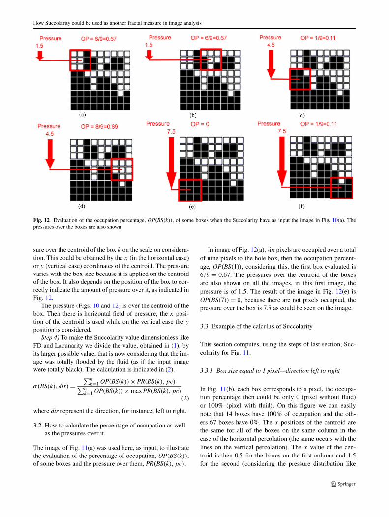
Fig. 12 Evaluation of the occupation percentage, OP(BS(k)), of some boxes when the Succolarity have as input the image in Fig. 10(a). Thepressures over the boxes are also shown

sure over the centroid of the box k on the scale on considera-tion. This could be obtained by the x (in the horizontal case)or y (vertical case) coordinates of the centroid. The pressurevaries with the box size because it is applied on the centroidof the box. It also depends on the position of the box to cor-rectly indicate the amount of pressure over it, as indicated inFig. 12.

The pressure (Figs. 10 and 12) is over the centroid of thebox. Then there is horizontal field of pressure, the x posi-tion of the centroid is used while on the vertical case the y

position is considered.Step 4) To make the Succolarity value dimensionless like

FD and Lacunarity we divide the value, obtained in (1), byits larger possible value, that is now considering that the im-age was totally flooded by the fluid (as if the input imagewere totally black). The calculation is indicated in (2).

σ(BS(k),dir) =∑n

k=1 OP(BS(k)) × PR(BS(k),pc)∑nk=1 OP(BS(k)) × max PR(BS(k),pc)

(2)

where dir represent the direction, for instance, left to right.

3.2 How to calculate the percentage of occupation as wellas the pressures over it

The image of Fig. 11(a) was used here, as input, to illustratethe evaluation of the percentage of occupation, OP(BS(k)),of some boxes and the pressure over them, PR(BS(k),pc).

In image of Fig. 12(a), six pixels are occupied over a totalof nine pixels to the hole box, then the occupation percent-age, OP(BS(1)), considering this, the first box evaluated is6/9 = 0.67. The pressures over the centroid of the boxesare also shown on all the images, in this first image, thepressure is of 1.5. The result of the image in Fig. 12(e) isOP(BS(7)) = 0, because there are not pixels occupied, thepressure over the box is 7.5 as could be seen on the image.

3.3 Example of the calculus of Succolarity

This section computes, using the steps of last section, Suc-colarity for Fig. 11.

3.3.1 Box size equal to 1 pixel—direction left to right

In Fig. 11(b), each box corresponds to a pixel, the occupa-tion percentage then could be only 0 (pixel without fluid)or 100% (pixel with fluid). On this figure we can easilynote that 14 boxes have 100% of occupation and the oth-ers 67 boxes have 0%. The x positions of the centroid arethe same for all of the boxes on the same column in thecase of the horizontal percolation (the same occurs with thelines on the vertical percolation). The x value of the cen-troid is then 0.5 for the boxes on the first column and 1.5for the second (considering the pressure distribution like

R.H.C. de Melo, A. Conci

Table 2 Results of the Succolarity of Fig. 8(a)

Succolarity (σ)

d BS b2t t2b l2r r2l

9 (1 × 1) 0.3429 0.2387 0.0384 0.4829

3 (3 × 3) 0.3292 0.2634 0.0576 0.4691

Fig. 10(b)). Figure 11(b) presents 7 boxes on the first col-umn and 7 more on the second. We have then using the nu-merator of (1) obtained the results 7 × 0.5 + 7 × 1.5 = 14.To compute the Succolarity we then divide this value bythe denominator of (2). This calculus results in 364.5(=9 × (0.5 + 1.5 + 2.5 + 3.5 + 4.5 + 5.5 + 6.5 + 7.5 + 8.5), asthe 9 columns suffer pressures between 0.5 to 8.5 and thereare 9 boxes on each column. The Succolarity value for thebox size 1 × 1 is then σ(1 × 1; l2r) = 14/364.5 ≈ 0.0384.

3.3.2 Box size equal to 9 pixels (3 × 3)—direction top tobottom

In Fig. 11(a) each box correspond to 3 × 3 pixels; to calcu-late the percentage of presence of each box is necessary todivide the number of filled pixels on the box by the area ofthat box (9 in this case). Figure 11(a) shows 7 boxes withsome percentage of occupation and 2 with 0%. The upperleft box has 6 pixels, the percentage of that boxes is then6/9 ≈ 0.67. The percentages of occupied boxes of the top ofthe image respectively from left to right are 0.67, 0.67 and0.56 (≈5/9), that is, a total of 1.90; on the middle boxesthis percentages are 0.11 (≈1/9),0.56 and 0.89 (≈8/9), atotal of 1.56; and on the bottom boxes there are 0, 0 and0.11. Considering the pressure like in Fig. 10(a), the y po-sition of the centroid is 1.5 on the three boxes of the top,4.5 on the three middle boxes and 7.5 on the 3 boxes onbottom of the image. The maximum value possible by a9 × 9 image with 3 × 3 boxes completely flooded is (1.5 +1.5 + 1.5 + 4.5 + 4.5 + 4.5 + 7.5 + 7.5 + 7.5) = 40.5. Thisvalue can be seen as the sum of the maximum “pressure”applied to each box. The Succolarity value is then easily de-termined by the simple application of (1). σ(3 × 3, t2b) ≈(1.5 × 1.90) + (4.5 × 1.56) + (7.5 × 0.11)/40.5 ≈ 0.2634.

All the results of the Succolarity of Fig. 8(a) are shownin Table 2.

3.4 Example of the 3D approach

Figure 13 shows the 3D synthetic image used to illustratethe approach of measuring the Succolarity of 3D images orobjects. In this image, the voxels are represented as cubes:yellow cubes (including the transparent ones) represent theobstacles to the fluid while the blue cubes already representthe areas where the fluid percolates the image. Figure 14

Fig. 13 3D Synthetic image used already with the representation ofthe percolation of fluid (in blue)

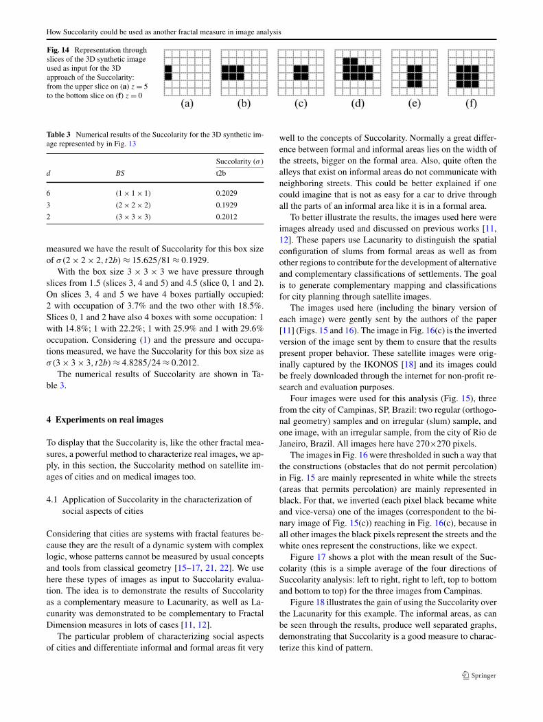
shows the 2D slices that forms the 3D synthetic image inFig. 13. In these images (Fig. 14), the black squares repre-sent the empty voxels corresponding to the paths that thefluid can flow from the top to the bottom slice of the image.The white squares represent the voxels in the image that cor-responds to the obstacles to the fluid flow through the image.

The pressure field through the new axis (z) grows fromtop to bottom, as represented in Fig. 13, then the pressureover the first slice (Fig. 14(a), z = 5) is smaller than the pres-sure on the second slice (Fig. 14(b), z = 4) and so on to thegreater pressure that is applied on the last slice (Fig. 14(f),z = 0).

The dimension of the image represented by the slices inFig. 13 is 6×6×6: 6 pixels wide; 6 pixels high and 6 pixelsdepth. This image has then three possibilities of division:factor of division 2, 3 or 6, having respectively boxes sizesof: 3 × 3 × 3; 2 × 2 × 2 and 1 × 1 × 1 pixels.

For the box of size 1 × 1 × 1 we have pressure valuesthrough the slices from 0.5 to 5.5. Considering “slice n” asthe slice where the value of z = n; the pressure is 5.5 onslice 0. Then we have 2 boxes with pressure 0.5 (slice 5); 6boxes with pressure 1.5 (slice 4); 4 boxes with pressure 2.5(slice 3); 10 slices with pressure 3.5 (slice 2); 6 boxes withpressure 4.5 (slice 1); and 9 boxes with pressure 5.5 (slice 0).Considering (1) and that with boxes of 1 × 1 × 1 the boxesare 0 or 100% occupied, the result of Succolarity for boxsize 1 × 1 × 1 is σ(1 × 1 × 1, t2b) ≈ 131.5/648 ≈ 0.2029.

For the box size 2 × 2 × 2 we have pressure throughslices from 1 (slice 4 and 5) to 5 (slice 0 and 1). On slices4 and 5 we have 2 boxes partially occupied: one with oc-cupation of 75% and the other with 25%. Slices 2 and 3(with pressure 3 over them) have 5 boxes with some occu-pation: 2 with 12.5%; 2 with 25% and 1 with 100% of oc-cupation. Slices 0 and 1 have 4 boxes partially occupied: 1with 12.5%; 1 with 25%; 1 with 50% and 1 with 100% of oc-cupation. Considering (1) and the pressure and occupations

How Succolarity could be used as another fractal measure in image analysis

Fig. 14 Representation throughslices of the 3D synthetic imageused as input for the 3Dapproach of the Succolarity:from the upper slice on (a) z = 5to the bottom slice on (f) z = 0

Table 3 Numerical results of the Succolarity for the 3D synthetic im-age represented by in Fig. 13

Succolarity (σ)

d BS t2b

6 (1 × 1 × 1) 0.2029

3 (2 × 2 × 2) 0.1929

2 (3 × 3 × 3) 0.2012

measured we have the result of Succolarity for this box sizeof σ(2 × 2 × 2, t2b) ≈ 15.625/81 ≈ 0.1929.

With the box size 3 × 3 × 3 we have pressure throughslices from 1.5 (slices 3, 4 and 5) and 4.5 (slice 0, 1 and 2).On slices 3, 4 and 5 we have 4 boxes partially occupied:2 with occupation of 3.7% and the two other with 18.5%.Slices 0, 1 and 2 have also 4 boxes with some occupation: 1with 14.8%; 1 with 22.2%; 1 with 25.9% and 1 with 29.6%occupation. Considering (1) and the pressure and occupa-tions measured, we have the Succolarity for this box size asσ(3 × 3 × 3, t2b) ≈ 4.8285/24 ≈ 0.2012.

The numerical results of Succolarity are shown in Ta-ble 3.

4 Experiments on real images

To display that the Succolarity is, like the other fractal mea-sures, a powerful method to characterize real images, we ap-ply, in this section, the Succolarity method on satellite im-ages of cities and on medical images too.

4.1 Application of Succolarity in the characterization ofsocial aspects of cities

Considering that cities are systems with fractal features be-cause they are the result of a dynamic system with complexlogic, whose patterns cannot be measured by usual conceptsand tools from classical geometry [15–17, 21, 22]. We usehere these types of images as input to Succolarity evalua-tion. The idea is to demonstrate the results of Succolarityas a complementary measure to Lacunarity, as well as La-cunarity was demonstrated to be complementary to FractalDimension measures in lots of cases [11, 12].

The particular problem of characterizing social aspectsof cities and differentiate informal and formal areas fit very

well to the concepts of Succolarity. Normally a great differ-ence between formal and informal areas lies on the width ofthe streets, bigger on the formal area. Also, quite often thealleys that exist on informal areas do not communicate withneighboring streets. This could be better explained if onecould imagine that is not as easy for a car to drive throughall the parts of an informal area like it is in a formal area.

To better illustrate the results, the images used here wereimages already used and discussed on previous works [11,12]. These papers use Lacunarity to distinguish the spatialconfiguration of slums from formal areas as well as fromother regions to contribute for the development of alternativeand complementary classifications of settlements. The goalis to generate complementary mapping and classificationsfor city planning through satellite images.

The images used here (including the binary version ofeach image) were gently sent by the authors of the paper[11] (Figs. 15 and 16). The image in Fig. 16(c) is the invertedversion of the image sent by them to ensure that the resultspresent proper behavior. These satellite images were orig-inally captured by the IKONOS [18] and its images couldbe freely downloaded through the internet for non-profit re-search and evaluation purposes.

Four images were used for this analysis (Fig. 15), threefrom the city of Campinas, SP, Brazil: two regular (orthogo-nal geometry) samples and on irregular (slum) sample, andone image, with an irregular sample, from the city of Rio deJaneiro, Brazil. All images here have 270×270 pixels.

The images in Fig. 16 were thresholded in such a way thatthe constructions (obstacles that do not permit percolation)in Fig. 15 are mainly represented in white while the streets(areas that permits percolation) are mainly represented inblack. For that, we inverted (each pixel black became whiteand vice-versa) one of the images (correspondent to the bi-nary image of Fig. 15(c)) reaching in Fig. 16(c), because inall other images the black pixels represent the streets and thewhite ones represent the constructions, like we expect.

Figure 17 shows a plot with the mean result of the Suc-colarity (this is a simple average of the four directions ofSuccolarity analysis: left to right, right to left, top to bottomand bottom to top) for the three images from Campinas.

Figure 18 illustrates the gain of using the Succolarity overthe Lacunarity for this example. The informal areas, as canbe seen through the results, produce well separated graphs,demonstrating that Succolarity is a good measure to charac-terize this kind of pattern.

R.H.C. de Melo, A. Conci

Fig. 15 Satellite images from IKONOS: (a) and (b) two regular samples of occupation from Campinas: (a) formal 1 and (b) formal 2; (c)informal 1: slum of Campinas; (d) informal 2: slum from Rio de Janeiro

Fig. 16 Binary version of images in Fig. 15

Fig. 17 Results of Succolarity medium obtained from the proposedmethod using as input the images of Campinas in Fig. 16(a) formal 1,(b) formal 2 and (c) informal 1

Another important point here, is that, this results are thearithmetic mean results of Succolarity in a way that, for spe-cific application, as we will see on the next section, onlyone or a particular number of directions could be mea-sured, as it are considered interesting for the problem to besolved.

On plots of Figs. 19 to 22 one could see that, throughother type of analysis, the results of Succolarity could beused to distinguish formal areas through informal ones.These results consider four directions that a fluid can floodthe original images: bottom to top (b2t); top to bottom (t2b);left to right (l2r); right to left (r2l). Figures 19 and 20 demon-

Fig. 18 Results of Succolarity medium obtained from the proposedmethod using as input the images of Campinas in Fig. 16(c) informal 1and 16 (d) informal 2

strate that, on formal areas, the results do not vary consid-erably with the direction. This is easily explained when wethink that formal areas usually have a great number of largestreets that go from lots of points to others including pointswhere some streets cross others.

Figures 21 and 22, which are results of Succolarity of in-formal areas, demonstrate that, in this kind of occupation,the direction used on the evaluation makes great impact onthe results. While, for the analyzed formal areas, the min-imum values of Succolarity evaluated are on decimals forthe informal areas, the minimum values are in hundredths,which is better seen next; in Tables 4, 5, 6 and 7 (the val-

How Succolarity could be used as another fractal measure in image analysis

Fig. 19 Results of Succolarity of the image in Fig. 16(a)—formal 1

Fig. 20 Results of Succolarity of the image in Fig. 16(b)—formal 2

Fig. 21 Results of Succolarity of the image in Fig. 16(c)—informal 1

ues on tables were multiplied by ten to make the valuesmore readable). Another consideration is that the maximumdifference between the measures that on formal areas arearound hundredths, in informal areas this difference growsconsiderably to decimals.

4.2 Application of Succolarity to medical images

An application of the Succolarity to vascular diagnosis isshown in this section. The two examples of images [14]demonstrate a carotid with and without occlusion. On first

Fig. 22 Results of Succolarity of the image in Fig. 16(d)—informal 2

Table 4 Numerical results of Succolarity of formal 1: Figs. 17 and 19

Succolarity (×10)

Dividing factor b2t t2b l2r r2l Medium

270 3.489 3.023 3.33 3.415 3.314

135 3.489 3.023 3.33 3.415 3.314

90 3.489 3.023 3.33 3.415 3.314

54 3.489 3.023 3.33 3.415 3.314

45 3.489 3.023 3.33 3.415 3.314

30 3.489 3.024 3.33 3.415 3.315

27 3.488 3.023 3.33 3.415 3.314

18 3.489 3.026 3.33 3.413 3.314

15 3.487 3.024 3.33 3.413 3.314

10 3.486 3.028 3.331 3.407 3.313

9 3.489 3.033 3.339 3.414 3.319

6 3.482 3.035 3.339 3.412 3.317

5 3.473 3.035 3.313 3.38 3.3

3 3.487 3.075 3.357 3.384 3.326

2 3.43 3.085 3.4 3.354 3.317

image named H53022B, Fig. 23, there is an internal carotidartery plaque, on the second H53031B, Fig. 24, there is aninternal carotid artery occlusion. Parts of the original imagethat contains only textual information were removed fromthe two images. The result images are both 480 × 240 pix-els.

In Figs. 23(a) and 23(b) it is not easy to visualize theocclusion that occurs in Fig. 24(b) and does not occur inFig. 24(a). These images were submitted to heuristic teststo determine good values of threshold. The results of thethreshold of these images are shown in Figs. 24(a) and 24(b).

After the threshold, it is easier to note that Fig. 24(b) hasa complete occlusion and Fig. 24(a) has a partial obstruc-tion. The next two images, Figs. 25(a) and 25(b), show theintermediate images generated during the executing of themethod proposed to calculate the Succolarity of the inputimage in Fig. 24(a).

R.H.C. de Melo, A. Conci

Table 5 Numerical results of Succolarity of formal 2: Figs. 17 and 20

Succolarity (×10)

Dividing factor b2t t2b l2r r2l Medium

270 3.432 3.364 2.752 3.152 3.175

135 3.432 3.364 2.752 3.152 3.175

90 3.432 3.364 2.752 3.152 3.175

54 3.432 3.364 2.752 3.152 3.175

45 3.432 3.364 2.751 3.152 3.175

30 3.431 3.364 2.753 3.152 3.175

27 3.432 3.364 2.752 3.151 3.175

18 3.431 3.364 2.753 3.151 3.175

15 3.428 3.362 2.754 3.152 3.174

10 3.424 3.361 2.754 3.147 3.172

9 3.415 3.354 2.756 3.148 3.168

6 3.41 3.355 2.758 3.145 3.167

5 3.408 3.358 2.755 3.139 3.165

3 3.326 3.294 2.783 3.121 3.131

2 3.295 3.286 2.847 3.113 3.135

Table 6 Numerical results of Succolarity of informal 1: Figs. 17, 18and 21

Succolarity (×10)

Dividing factor b2t t2b l2r r2l Medium

270 2.87 0.543 0.317 3.113 1.711

135 2.87 0.543 0.317 3.113 1.711

90 2.87 0.543 0.317 3.113 1.711

54 2.87 0.543 0.318 3.113 1.711

45 2.87 0.543 0.317 3.113 1.711

30 2.869 0.543 0.318 3.113 1.711

27 2.869 0.544 0.319 3.112 1.711

18 2.868 0.546 0.321 3.111 1.711

15 2.866 0.547 0.322 3.112 1.712

10 2.861 0.553 0.327 3.113 1.711

9 2.862 0.556 0.333 3.104 1.714

6 2.845 0.568 0.35 3.086 1.712

5 2.828 0.574 0.358 3.107 1.717

3 2.765 0.645 0.424 3.03 1.716

2 2.595 0.823 0.637 2.867 1.73

The two following images, Figs. 26(a) and 26(b), showthe intermediate images generated during the executing ofthe method proposed to calculate the Succolarity for the in-put image in Fig. 24(b).

The ln× ln plots of the Succolarity are shown in Figs. 27and 28.

Table 8 shows the Succolarity numerical values for theimage H53022B, Fig. 23(a). Table 9 shows the Succolaritynumerical values for the image H53031B, Fig. 23(b).

Table 7 Numerical results of Succolarity of informal 2: Figs. 18 and22

Succolarity (×10)

Dividing factor b2t t2b l2r r2l Medium

270 1.768 0.189 0.332 0.469 0.69

135 1.768 0.189 0.332 0.469 0.69

90 1.768 0.189 0.332 0.469 0.69

54 1.768 0.19 0.332 0.469 0.69

45 1.768 0.19 0.333 0.468 0.69

30 1.767 0.19 0.333 0.468 0.69

27 1.767 0.191 0.333 0.468 0.69

18 1.765 0.19 0.334 0.467 0.689

15 1.764 0.193 0.336 0.466 0.69

10 1.757 0.195 0.336 0.463 0.688

9 1.757 0.199 0.334 0.461 0.688

6 1.742 0.207 0.349 0.453 0.688

5 1.723 0.217 0.358 0.448 0.686

3 1.6 0.234 0.373 0.414 0.655

2 1.44 0.287 0.47 0.373 0.642

Table 8 Numerical values of Succolarity of the threshold H53022B,Fig. 23(a). d is the factor of division, BS, the box size (width × height)

Succolarity (σ) ln(100 × σ)

d ln(d) BS l2r r2l l2r r2l

8 2.0794 (30 × 17) 0.4014 0.4169 3.6924 3.7303

4 1.3863 (60 × 34) 0.3993 0.4138 3.6871 3.7228

2 0.6931 (120 × 68) 0.3913 0.4036 3.6669 3.6978

Table 9 Numerical values of Succolarity of the threshold H53031B,Fig. 23(b). d is the factor of division, BS, the box size (width × height)

Succolarity (σ) ln(100 × σ)

d ln(d) BS l2r r2l l2r r2l

4 1.3863 (61 × 34) 0.1631 0.4306 2.7918 3.7626

2 0.6931 (122 × 68) 0.188 0.4181 2.9339 3.7331

The direction considered on the results was only horizon-tal because the vessels on the images are on this direction.In the non occluded image the results on the curve to l2r andr2l almost match as we can see by Fig. 27. However, whenan obstacle is present on the analyzed image, the l2r and r2lcurves differs significantly as could be seen in Fig. 28.

5 Conclusion

In this work, an approach to evaluate the fractal measureof Succolarity was presented. An equation to evaluate thismeasure was proposed based on the notions of directional

How Succolarity could be used as another fractal measure in image analysis

Fig. 23 Carotid images fromthe vascular-web database [14]:(a) H53022B—Internal carotidartery plaque; and (b)H53031B—Internal carotidartery occlusion

Fig. 24 Thresholded images ofimages in Fig. 23: (a) Value ofthreshold heuristically chosenwas 18; and (b) Value ofthreshold heuristically chosenwas 15

Fig. 25 Intermediate imagesfrom the processing of image inFig. 24(a): (a) for the directionleft to right (l2r); and (b) for thedirection right to left (r2l)

Fig. 26 Intermediate imagesfrom the processing of image inFig. 24(b) (a) for the directionleft to right (l2r); and (b) for thedirection right to left (r2l)

pressure due to percolation of a fluid in a partially penetrableenvironment.

How to compute the Succolarity from binary 2D and 3Ddigital images were discussed through examples.

Like the Lacunarity, our proposal to Succolarity compu-tation considers the use of bi logarithm (ln× ln) or linear× log plots instead of a single value. The Succolarity val-ues over different box sizes could give essential informationuseful to the pattern recognition process.

The results of the experiments on real images show thatthe method is very useful as a new feature to integrate othercharacteristics on pattern recognition processes. The notionsof Succolarity [1] were respected and the measure could be

seen as a natural evolution of the FD and Lacunarity. Theother advantage of the method is to be simple, easy and fastto be calculated.

The analysis of satellite images of cities over its social as-pects using the Lacunarity is better than using FD [11, 12].The method proposed here describes another approach thatcould differentiate not only between formal and informal ar-eas like does the Lacunarity in [11, 12], but between differ-ent kinds of informal areas too.

The analysis of the vascular medical images indicatesthat the Succolarity is useful on determining vascular ob-structions in ultrasound exams and strength the argument

R.H.C. de Melo, A. Conci

Fig. 27 ln× ln plot of the Succolarity for Fig. 24(a)

Fig. 28 ln× ln plot of the Succolarity for Fig. 24(b)

that directional information on images could be very wellextracted by this method.

The main gain of using the Succolarity is that the methodenables not one, but lots of ways to analyze the results, ascould be seen by the two kinds of applications in this work,once the user knows something about what kind of informa-tion he wants to extract from the image, more he can takeadvantage of the representation of the result. The user coulduse different directions, combining it or not, depending onthe problem in question. These were illustrated by the citiesresults of Succolarity, which uses four directions, and thevascular medical images results, that use only two direc-tions. Succolarity is a great measure, which is very useful,not only for the type of images used here, but to genericimages, that present some information associated with di-rection or flow. Among the applications are the study of per-colation of petroleum and natural gas through semi-porousrock; where the theory can help to predict and improve theproductivity of natural gas and oil.

Acknowledgements This work has been supported by CAPES, theBrazilian government agency.

References

1. Mandelbrot, B. B. (1977). Fractal geometry of nature. New York:Freeman.

2. Melo, R. H. C. (2007). Using fractal characteristics such as frac-tal dimension, Lacunarity and Succolarity to characterize texturepatterns on images. Master’s thesis, Federal Fluminense Univer-sity. Link: http://www.ic.uff.br/~rmelo/msc_thesis.htm.

3. Melo, R. H. C., Vieira, E. A., & Conci, A. (2006). Comparingtwo approaches to compute Lacunarity of mammograms. In Pro-ceedings of the IEEE signal processing society 13th internationalconference on systems, signal and image processing and semanticmultimodal analysis of digital media (IWSSIP 2006), Budapest,Hungary (pp. 299–302).

4. Melo, R. H. C., Vieira, E. A., & Conci, A. (2006). Characterizingthe Lacunarity of objects and image sets and its use as a techniquefor the analysis of textural patterns. In J. Blanc-Talon, et al. (Eds.),LNCS: Vol. 4179. Advanced concepts for intelligent vision systems(pp. 208–219). Berlin: Springer.

5. Sarkar, N., & Chaudhuri, B. B. (1992). An efficient approach toestimate Fractal Dimension of textural images. Pattern Recogni-tion, 25, 1035–1041.

6. Block, A., von Bloh, W., & Schellnhuber, H. J. (1990). Efficientbox-counting determination of generalized Fractal Dimensions.Physical Review. A, 42, 1869–1874.

7. Barabási, A. L., & Stanley, H. E. (1995). Fractal concepts in sur-face growth. New York: Cambridge University Press.

8. Conci, A., & Monteiro, L. H. (2000). Multifractal characterizationof texture-based segmentation. In ICIP 2000, Vancouver, Canada(pp. 792–795).

9. Conci, A., & Proença, C. B. (1998). In Computer networks andISDN Systems, pages: Vol. 30. A fractal image analysis systemfor fabric inspection based on a box-counting method (pp. 1887–1895). Amsterdam: Elsevier.

10. Mandelbrot, B. B., & Van Ness, J. (1968). Fractional Brownianmotion, fractional noise and applications. SIAM Review, 10, 422–437.

11. Barros Filho, M. N. M., & Sobreira, F. A. (2005). Assessing texturepattern in slums across scales: an unsupervised approach. CASAworking paper, Centre for Advanced Spatial Analysis, CASASeminar, University College London, London, 87. Link: http://www.casa.ucl.ac.uk/working_papers/paper87.pdf.

12. Barros Filho, M. N. M., & Sobreira, F. A. (2005). Analysing spa-tial patterns in slums: a multiscale approach. Congresso Interna-cional de Planejamento Urbano Regional Integrado e Sustentável,São Carlos (SP). São Carlos: PLURIS.

13. Melo, R. H. C., & Conci, A. (2008). Succolarity: defining amethod to calculate this fractal measure. In 15th internationalconference systems, signals and image processing, 2008. IWSSIP2008, Bratislava, Slovak Republic (pp. 291–294).

14. Size, G. P., & Duncan, R. K. (2006). Vascular-web. Link: http://www.vascular-web.com, 2006.

15. Batty, M., & Longley, P. (1994). Fractal cities: geometry of formand function (1st ed.). London: Academic Press.

16. Frankhauser, P. (1997). Fractal analysis of urban structures. In E.Holm (Ed.), Modelling space and networks: progress in theoreti-cal and quantitative geography (pp. 145–181). Umea: Gerum Kul-turgeografi.

17. Sobreira, F., & Gomes, M. (2001). The geometry of slums: bound-aries, packing and diversity. Working paper series, CASA—Centre for Advanced Spatial Analysis—University CollegeLondon, London, 30. Link: http://www.casa.ucl.ac.uk/working_papers/paper30.pdf.

18. Space Imaging Brazil (2004). Link: http://www.spaceimaging.com.br/.

19. Barros Filho, M. N. M., & Sobreira, F. J. A. (2008). Accuracyof Lacunarity algorithms in texture classification of high spatialresolution images from urban areas. In XXI congress of interna-tional society of photogrammetry and remote sensing, 2008, Bei-jing, China. XXI congress of international society of photogram-metry and remote sensing, Beijing, China.

How Succolarity could be used as another fractal measure in image analysis

20. Valous, N. A., Mendoza, F., Sun, D.-W., & Allen, P. (2009). Tex-ture appearance characterization of pre-sliced pork ham imagesusing fractal metrics: Fourier analysis dimension and Lacunarity.Food Research International, 42(3), 353–362.

21. Frankhauser, P. (2008). Fractal geometry for measuring and mod-elling urban patterns. In S. Albeverio, D. Andrey, P. Giordano, &A. Vancheri (Eds.), The dynamics of complex urban systems—aninterdisciplinary approach (pp. 241–243). Berlin: Springer.

22. Tannier, C., & Pumain, D. (2005). Fractals in urban geography:a theoretical outline and an empirical example, Cybergeo. Eu-ropean Journal of Geography, 307, 20 http://www.cybergeo.eu/index3275.html, 22 pp.

R.H.C. de Melo received his M.Sc.in Computer Science from Fed-eral Fluminense University (UFF)at Niterói (Brazil) in 2007. He iscurrently a project manager and re-searcher at ADDLabs (The Artifi-cial Intelligent laboratory of UFF).His major research interest includesimage processing, image analysis,pattern recognition and computervision (https://sites.google.com/site/rhcmelo/).

A. Conci received M.Sc. and D.Sc.degrees in civil engineering fromPUC-Rio, Brazil, in 1983 and 1988,respectively. Since 1994 she hasbeen a titular professor at the Fed-eral Fluminense University, first inMechanical Engineer Departmentand now in Computer Science De-partment. Her major research inter-ests are in Computer Graphics, Im-age Processing and Biomechanics(http://www.ic.uff.br/~aconci).