housing market spillovers: evidence from an estimated … · 126 american economic journal:...
TRANSCRIPT

125
American Economic Journal: Macroeconomics 2 (April 2010): 125–164http://www.aeaweb.org/articles.php?doi=10.1257/mac.2.2.125
The experience of the US housing market at the beginning of the twenty-first century (fast growth in housing prices and residential investment initially, and
a decline thereafter) has led many to raise the specter that the developments in the housing sector are not just a passive reflection of macroeconomic activity, but might be one of the driving forces of business cycles. To understand whether such concerns are justified, it is crucial to answer two questions. What is the nature of the shocks hitting the housing market? And, how big are the spillovers from the housing market to the wider economy?
In this paper, we address these questions using a quantitative approach. We develop and estimate, using Bayesian methods, a dynamic stochastic general equilibrium model of the US economy that explicitly models the price and the quantity side of the housing market. Our goal is twofold. First, we want to study the combination of shocks and frictions that can explain the dynamics of residential investment and housing prices in the data. Second, to the extent that the model can reproduce key features of the data, we want to measure the spillovers from the housing market to the wider economy. Our starting point is a variant of many dynamic equilibrium models with a neoclassical core and nominal and real rigidities that have become popular in monetary policy analysis (see Lawrence J. Christiano, Martin Eichenbaum, and
* Iacoviello: Boston College, Department of Economics, 140 Commonwealth Ave, Chestnut Hill, MA, 02467 (e-mail: [email protected]); Neri: Banca d’Italia, Research Department, Via Nazionale 91, 00184 Roma, Italy (e-mail: [email protected]). The views expressed in this paper are those of the authors and do not nec-essarily reflect the views of the Banca d’Italia. We thank two anonymous referees, Richard Arnott, Zvi Eckstein, Jesus Fernandez-Villaverde, Jonas Fisher, Jordi Galí, Peter Ireland, Michel Juillard, Bob King, Gabriel Lee, Lisa Lynch, Caterina Mendicino, Tommaso Monacelli, John Muellbauer, Fabio Schiantarelli, Livio Stracca, Karl Walentin, and conference and seminar participants for comments and suggestions.
† To comment on this article in the online discussion forum, or to view additional materials, visit the articles page at http://www.aeaweb.org/articles.php?doi=10.1257/mac.2.2.125.
Housing Market Spillovers: Evidence from an Estimated DSGE Model †
By Matteo Iacoviello and Stefano Neri*
We study sources and consequences of fluctuations in the US housing market. Slow technological progress in the housing sector explains the upward trend in real housing prices of the last 40 years. Over the busi-ness cycle, housing demand and housing technology shocks explain one-quarter each of the volatility of housing investment and housing prices. Monetary factors explain less than 20 percent, but have played a bigger role in the housing cycle at the turn of the century. We show that the housing market spillovers are nonnegligible, concentrated on consumption rather than business investment, and have become more important over time. (JEL E23, E32, E44, O33, R31)
ContentsHousing Market Spillovers: Evidence from an Estimated DSGE Model † 125
I. The Model 128A. Households 128B. Technology 131C. Nominal Rigidities and Monetary Policy 131D. Equilibrium 133E. Trends and Balanced Growth 133II. Parameter Estimates 134A. Methods and Data 134B. Calibrated Parameters 136C. Prior Distributions 138D. Posterior Distributions 139III. Properties of the Estimated Model 140A. Impulse Responses 140B. Cyclical Properties 144C. Robustness Analysis 144IV. Sources and Consequences of Housing Market Fluctuations 147A. What Drives the Housing Market? 147B. How Large Are the Spillovers from the Housing Market? 153V. Concluding Remarks 156References 163
126 AMEricAn EcOnOMic JOUrnAL: MAcrOEcOnOMicS ApriL 2010
Charles L. Evans 2005; and Frank Smets and Rafael Wouters 2007). There are at least two reasons why we regard these models (that do not consider housing explic-itly) as our starting point. First, because the goal is to study the interactions between housing and the broader economy, it is natural to have as a benchmark a model that fits the US data well on the one hand,1 and that encompasses most of the views on the sources and propagation mechanism of business cycles on the other hand. Second, because our housing model (aside from minor differences) encompasses the core of these models as a special case, it can facilitate communication to policymak-ers and between researchers.
Our model captures two main features of housing. On the supply side, we add sectoral heterogeneity, as in Morris A. Davis and Jonathan Heathcote (2005). The nonhousing sector produces consumption and business investment using capital and labor; and the housing sector produces new homes using capital, labor, and land. On the demand side, housing and consumption enter households’ utility, and hous-ing can be used as collateral for loans, as in Iacoviello (2005). Since housing and consumption goods are produced using different technologies, the model generates endogenous dynamics both in residential vis-à-vis business investment and in the price of housing. At the same time, fluctuations in house prices affect the borrowing capacity of a fraction of households, on the one hand, and the relative profitability of producing new homes, on the other hand. These mechanisms generate feedback effects for the expenditure of households and firms.2
We estimate the model using quarterly data over the period 1965:QI–2006:QIV. The dynamics of the model are driven by productivity, and nominal and prefer-ence shocks. Our estimated model explains several features of the data well. It can explain the cyclical properties and the long-run behavior of housing and nonhousing variables. It can also match the observation that both housing prices and housing investment are strongly procyclical, volatile, and very sensitive to monetary shocks. In terms of the two questions we posed at the beginning, we conclude that:
• Over long horizons, the model can explain, qualitatively and quantitatively, the trends in real housing prices and investment of the last four decades. The increase in real housing prices is the consequence of slower technological prog-ress in the housing sector and of the presence of land (a fixed factor) in the production function for new homes. Over the business cycle, three main factors drive the housing market. Housing demand and housing supply shocks explain roughly one-quarter each of the cyclical volatility of housing investment and housing prices. Monetary factors explain between 15 and 20 percent of the cyclical volatility of housing investment and housing prices. Looking at the historical decomposition, we find that the housing cycles of the late 1970s/early 1980s had a relatively strong technological component, whereas the housing
1 See, for instance, Marco Del Negro et al. (2007).2 We model the housing market as a single national market. Obviously, there is a strong regional component
to house prices. However, there are no big differences between regional components of gross domestic product (GDP) and regional components of house prices. To give a quantitative flavor, the first principal component of annual GDP growth for the 8 BEA regions explains 55 percent of GDP growth for the period 1976–2007. For real house prices in the corresponding census regions, the corresponding number is 53 percent.

VOL. 2 nO. 2 127iAcOViELLO And nEri: hOUSing MArkEt SpiLLOVErS
cycles at the turn of the twenty-first century were driven in nonnegligible part by monetary factors.
• There is not a unique way of quantifying housing market spillovers since, obviously, both housing prices and quantities are endogenous variables in our model. We focus on one aspect of the spillovers, that is, the relationship between housing wealth and nonhousing consumption. We find that collateral effects on household borrowing amplify the response of nonhousing consump-tion to given changes in fundamentals, thus altering the propagation mecha-nism. In Section IV, we find that our estimated collateral effects increase the reduced-form elasticity of consumption to housing wealth by 2.5 percentage points, from about 0.11 to 0.135. In addition, when we estimate the model over two subsamples, before and after the 1980s, we show that housing collateral effects have contributed to 6 percent of the variance in consumption growth in the early period, and to 12 percent of the variance in consumption growth in the late period. Hence, the average spillovers from the housing market to the rest of the economy have become more important over time.3
Our analysis combines four main elements: (i) a multi-sector structure with housing and nonhousing goods; (ii) nominal rigidities; (iii) financing frictions in the household sector; and (iv) a rich set of shocks, which are essential to take the model to the data.4 Jeremy Greenwood and Zvi Hercowitz (1991); Jess Benhabib, Richard Rogerson, and Randall Wright (1991); Yongsung Chang (2000); Davis and Heathcote (2005); and Jonas D. M. Fisher (2007) are examples of calibrated models dealing with (i), but they consider only technology shocks. Davis and Heathcote (2005) is perhaps our closest antecedent, since their multi-sector struc-ture endogenizes both housing prices and quantities in an equilibrium framework. They use a model with intermediate goods in which construction, manufacturing, and services are used to produce consumption, business investment, and struc-tures. Structures are then combined with land to produce homes. On the supply side, our setup shares some features with theirs. However, since our goal is to take the model to the data, we allow additional real and nominal frictions and a larger set of shocks. There are three advantages in doing so. First, we do not need to commit to a particular view of sources of business cycle fluctuations. Indeed, our results show that several shocks are needed to explain the patterns of comovement observed in the data. Second, we can analyze the monetary trans-mission mechanism to housing prices and housing investment. Third, we can do a better job of explaining the interactions between housing and macroeconomy. For instance, Davis and Heathcote (2005) require sectoral technology shocks to
3 In our variance decomposition, we also show that the direct effect on the economy of housing-specific shocks is small. A large fraction of what we identify as housing spillovers thus reflects the role of housing in propagating other shocks, rather than shocks originating in the housing market itself.
4 Several papers have studied the role of housing collateral in models with incomplete markets and financing frictions by combining elements of (i) and (iii). See, for instance, Martin Gervais (2002); Brian Peterson (2006); Antonia Díaz and Maria Jose Luengo-Prado (forthcoming); and François Ortalo-Magné and Sven Rady (2006). These papers, however, abstract from aggregate shocks.

128 AMEricAn EcOnOMic JOUrnAL: MAcrOEcOnOMicS ApriL 2010
explain the high volatility of housing investment: However, these shocks also yield the counterfactual prediction that housing prices and housing investment are nega-tively correlated.5
I. The Model
The model features two sectors, heterogeneity in households’ discount factors and collateral constraints tied to housing values. On the demand side, there are two types of households: patient (lenders) and impatient (borrowers). Patient households work, consume, and accumulate housing. They own the productive capital of the economy, and supply funds to firms on the one hand, and to impatient households on the other hand. Impatient households work, consume, and accumulate housing. Because of their high impatience, they accumulate only the required net worth to finance the down payment on their home and are up against their housing collateral constraint in equilibrium. On the supply side, the nonhousing sector combines capital and labor to produce consumption and business capital for both sectors. The housing sector produces new homes combining business capital with labor and land.
A. households
There is a continuum of measure 1 of agents in each of the two groups (patient and impatient). The economic size of each group is measured by its wage share, which is assumed to be constant through a unit elasticity of substitution production function. Within each group, a representative household maximizes:6
(1) E0 ∑ t=0
∞ (βgc)t zt aΓc ln(ct − εct−1 ) + jt lnht − τt ____
1 +η An c, t 1+ξ + n h, t 1+ξ B 1+η ____
1+ξ b ;
(2) E0 ∑ t=0
∞ (β′gc)t zt aΓ′c ln(c′t − ε′c′t−1) + jt lnh′t −
τt ____ 1+η′ A(n′c, t )1+ξ′ + (n′h, t )1+ξ′ B 1+η′ ____
1+ξ′ b .
Variables without (with) a prime refer to patient (impatient) households. c, h, nc , and nh are consumption, housing, hours in the consumption sector, and hours in the hous-ing sector. The discount factors are β and β′ (β′ < β ). The terms zt and τt capture shocks to intertemporal preferences and to labor supply.
We label movements in jt as housing preference shocks. There are at least two possible interpretations of this shock. One interpretation is that the shock captures, in a reduced form way, cyclical variations in the availability of resources needed to purchase housing relative to other goods or other social and institutional changes
5 Rochelle M. Edge, Michael T. Kiley, and Jean-Philippe Laforte (2007) integrate (i), (ii), and (iv) by distin-guishing between two production sectors and between consumption of nondurables and services, investment in durables and in residences. Hafedh Bouakez, Emanuela Cardia, and Francisco J. Ruge-Murcia (2009) estimate a model with heterogenous production sectors that differ in price stickiness, capital adjustment costs, and produc-tion technology. None of these papers deal explicitly with housing prices and housing investment, which are the main focus of our analysis.
6 We assume a cashless limit in the sense of Michael Woodford (2003).

VOL. 2 nO. 2 129iAcOViELLO And nEri: hOUSing MArkEt SpiLLOVErS
that shift preferences toward housing. Another interpretation is that fluctuations in jt could proxy for random changes in the factor mix required to produce home services from a given housing stock.7 The shocks follow
ln zt = ρz ln zt−1 + uz, t ; ln τt = ρτ ln τt−1 + uτ, t ;
ln jt = (1 − ρj ) ln j + ρj ln jt−1 + uj, t ,
where uz, t, uτ, t , and uj, t are independently and identically distributed processes with variances σ z 2 , σ τ 2 , and σ j
2 . Above, ε measures habits in consumption,8 and gc is the growth rate of consumption in the balanced growth path. The scaling factors Γc = (gc − ε)/(gc − βεgc) and Γ ′c = (gc − ε′ )/(gc − β′ε′gc) ensure that the marginal utilities of consumption are 1/c and 1/c′ in the steady state.
The log-log specification of preferences for consumption and housing reconciles the trend in the relative housing prices and the stable nominal share of expenditures on household investment goods, as in Davis and Heathcote (2005) and Fisher (2007). The specification of the disutility of labor (ξ, η ≥ 0) follows Michael Horvath (2000) and allows for less than perfect labor mobility across sectors. If ξ and ξ′ equal zero, hours in the two sectors are perfect substitutes. Positive values of ξ and ξ′ (as Horvath found) allow for some degree of sector specificity and imply that relative hours respond less to sectoral wage differentials.
Patient households accumulate capital and houses and make loans to impatient households. They rent capital to firms, choose the capital utilization rate, and sell the remaining undepreciated capital. In addition, there is joint production of con-sumption and business investment goods. Patient households maximize their utility subject to
ct + kc, t ___ Ak, t
+ kh, t + kb, t + qt ht + pl, t lt − bt = wc, t nc, t _____
Xwc, t +
wh, t nh, t _____ Xwh, t
+ arc, t zc, t + 1 − δkc ______ Ak, t
b kc, t−1 + (rh, t zh, t + 1 − δkh)kh, t−1 +pb, t kb, t − rt−1 bt−1 ______ πt
+ ( pl, t + rl, t)lt−1 + qt (1 − δh)ht−1 + divt −ϕ t − a(zc, t)kc, t−1 _
Ak, t − a(zh, t)
kh, t−1.
Patient agents choose consumption ct , capital in the consumption sector kc, t , capi-tal kh, t and intermediate inputs kb, t (priced at pb, t ) in the housing sector, housing ht
7 To see why, consider a simplified home technology producing home services through sst = h t κt , where κt is a time-varying elasticity of housing services sst to the housing stock ht, holding other inputs constant. This time-varying elasticity could reflect short-run fluctuations in the housing input required to produce a given unit of housing services. If the utility depends on the service flow from housing, this home technology shock looks like a housing preference shock in the reduced-form utility function.
8 The specification we adopt allows for habits in consumption only. In preliminary estimation attempts, we allowed for habits in housing and found no evidence of them.

130 AMEricAn EcOnOMic JOUrnAL: MAcrOEcOnOMicS ApriL 2010
(priced at qt ), land lt (priced at pl, t ), hours nc, t and nh, t , capital utilization rates zc, t and zh, t , and borrowing bt (loans if bt is negative) to maximize utility subject to (3). The term Ak, t captures investment-specific technology shocks, thus represent-ing the marginal cost (in terms of consumption) of producing capital used in the nonhousing sector.9 Loans are set in nominal terms and yield a riskless nominal return of rt. Real wages are denoted by wc, t and wh, t , real rental rates by rc, t and rh, t , and depreciation rates by δkc and δkh. The terms Xwc, t and Xwh, t denote the markup (due to monopolistic competition in the labor market) between the wage paid by the wholesale firm and the wage paid to the households, which accrues to the labor unions (below, we discuss the details of nominal rigidities in the labor market). Finally, πt = pt/pt−1 is the money inflation rate in the consumption sector, divt are lump-sum profits from final good firms and from labor unions, ϕt denotes convex adjustment costs for capital, z is the capital utilization rate that transforms physical capital k into effective capital z k, and a(·) is the convex cost of setting the capital utilization rate to z. The equations for ϕt , a(·), and divt are in Appendix B.10
Impatient households do not accumulate capital and do not own finished good firms or land (their dividends come only from labor unions). In addition, their maxi-mum borrowing b′t is given by the expected present value of their home times the loan-to-value (LTV) ratio m:11
(4) c′t + qt h ′t − b′t = w′c, t n′c, t/X ′wc, t + w′h, t n′h, t _____
X′wh, t + qt (1 − δh)h′t−1 − rt−1 b′t−1 ______ πt
+ div′t ;
(5) b′t ≤ mEt aqt+1 h′t πt+1 ________ rt
b .
The assumption β ′ < β implies that for small shocks the constraint (5) holds with equality near the steady state. When β ′ is lower than β, impatient agents decumulate wealth quickly enough to some lower bound and, for small shocks, the lower bound is binding.12 Patient agents own and accumulate all the capital. Impatient agents only
9 We assume that investment shocks hit only the capital used in the production of consumption goods, kc, since investment-specific technological progress mostly refers to information technology (IT), and construction is a non-IT-intensive industry.
10 We do not allow for a convex adjustment cost of housing demand (in preliminary estimation attempts, we found that the parameter measuring this cost was driven to its lower bound of zero). Home purchases are subject to nonconvex adjustment costs (typically, some fixed expenses and an agent fee that is proportional to the value of the house), which cannot be dealt with easily in our model. It is not clear whether these nonconvex costs bear important implications for aggregate residential investment. For instance, Julia K. Thomas (2002) finds that infrequent microeconomic adjustment at the plant level has negligible implications for the behavior of aggregate investment. In addition, a sizable fraction (25 percent) of residential investment in the National Income and Product Accounts consists of home improvements, where transaction costs are less likely to apply.
11 An analogous constraint might apply to patient households too, but would not bind in equilibrium.12 The extent to which the borrowing constraint holds with equality in equilibrium mostly depends on the
difference between the discount factors of the two groups and on the variance of the shocks that hit the economy. We have solved simplified, nonlinear versions of two-agent models with housing and capital accumulation in the presence of aggregate risk that allow for the borrowing constraint to bind only occasionally. For discount rate dif-ferentials of the magnitude assumed here, impatient agents are always arbitrarily close to the borrowing constraint (details are available upon request). For this reason, we solve the model linearizing the equilibrium conditions of the model around a steady state with a binding borrowing constraint.

VOL. 2 nO. 2 131iAcOViELLO And nEri: hOUSing MArkEt SpiLLOVErS
accumulate housing and borrow the maximum possible amount against it. Along the equilibrium path, fluctuations in housing values affect, through (5), borrowing and spending capacity of constrained households. The effect is larger the larger m, since m measures, ceteris paribus, the liquidity of housing wealth.
B. technology
To introduce price rigidity in the consumption sector, we differentiate between competitive flexible price/wholesale firms that produce wholesale consumption goods and housing using two technologies, and a final good firm (described below) that operates in the consumption sector under monopolistic competition. Wholesale firms hire labor and capital services, and purchase intermediate goods to produce wholesale goods Yt and new houses iht. They solve:
max Yt __ Xt
+ qt iht − a∑ i=c, h
wi, t ni, t + ∑ i=c, h
w ′i, t n′i, t + ∑ i=c, h
ri, t zi, t ki, t−1
+ rl, t lt−1 + pb, t kb, t b .
Above, Xt is the markup of final goods over wholesale goods. The production tech-nologies are:
(6) Yt = AAc, t ( n c, t α n ′ c, t
1−α ) B 1−μc (z c, t k c, t−1 ) μc ;
(7) i ht = AAh, t ( n h, t α n ′ h, t
1−α ) B 1−μh−μb−μl (zh, t kh, t−1 ) μh k b, t μb l t−1
μl .
In (6), the nonhousing sector produces output with labor and capital. In (7), new homes are produced with labor, capital, land, and the intermediate input kb. The terms Ac, t and Ah, t measure productivity in the nonhousing and housing sector, respectively.
As shown by (6) and (7), we let hours of the two households enter the two produc-tion functions in a Cobb-Douglas fashion. This assumption implies complementarity across the labor skills of the two groups and allows obtaining closed-form solutions for the steady state of the model. With this formulation, the parameter α measures the labor income share of unconstrained households.13
C. nominal rigidities and Monetary policy
We allow for price rigidities in the consumption sector and for wage rigidities in both the consumption and housing sectors. We rule out price rigidities in the
13 We have experimented with an alternative setup in which hours of the groups are perfect substitutes in pro-duction, with similar results. The alternative formulation is analytically less tractable, since it implies that hours worked by one group will affect total wage income received by the other group, thus creating a complex interplay between borrowing constraints and labor supply decisions of both groups.
132 AMEricAn EcOnOMic JOUrnAL: MAcrOEcOnOMicS ApriL 2010
housing market. According to Robert B. Barsky, Christopher L. House, and Miles S. Kimball (2007), there are several reasons why housing might have flexible prices. First, housing is relatively expensive on a per-unit basis. Therefore, if menu costs have important fixed components, there is a large incentive to negotiate on the price of this good. Second, most homes are priced for the first time when they are sold.
We introduce sticky prices in the consumption sector by assuming monopolistic competition at the “retail” level and implicit costs of adjusting nominal prices fol-lowing Calvo-style contracts. Retailers buy wholesale goods Yt from wholesale firms at the price p t
w in a competitive market, differentiate the goods at no cost, and sell them at a markup Xt = p t / p t
w over the marginal cost. The CES aggregates of these goods are converted back into homogeneous consumption and investment goods by households. Each period, a fraction 1 − θπ of retailers set prices optimally, while a fraction θπ cannot do so, and index prices to the previous period inflation rate with an elasticity equal to ιπ . These assumptions deliver the following consumption-sector Phillips curve:
(8) ln πt − ιπ ln πt−1 = βgc(Et ln πt+1 − ιπ ln πt) − επ ln (Xt/X ) + up, t ,
where επ = (1 − θπ)(1 − βgc θπ)/θπ . Above, independently and identically distrib-uted cost shocks up, t are allowed to affect inflation independently from changes in the markup. These shocks have zero mean and variance σ p 2 .
We model wage setting in a way that is analogous to price setting. Patient and impatient households supply homogeneous labor services to unions. The unions dif-ferentiate labor services as in Smets and Wouters (2007), set wages subject to a Calvo scheme and offer labor services to wholesale labor packers who reassemble these services into the homogeneous labor composites nc, nh, n′c , and n′h.14 Wholesale firms hire labor from these packers. Under Calvo pricing with partial indexation to past inflation, the pricing rules set by the union imply four wage Phillips curves that are isomorphic to the price Phillips curve. These equations are in Appendix B.
To close the model, we assume that the central bank sets the interest rate rt according to a Taylor rule that responds gradually to inflation and GDP growth:15
(9) rt = r t−1 rr π t (1−rr)rπ a gdpt ________
gc gdpt−1 b
(1−rr)rY
__
rr 1−rr ur, t ___ st
.
Above, __
rr is the steady-state real interest rate; ur, t is an independently and identically distributed monetary shock with variance σ r 2 ; st is a stochastic process with high
14 We assume that there are four unions, one for each sector/household pair. While unions in each sector choose slightly different wage rates, reflecting the different consumption profiles of the two household types, we assume that the probability of changing wages is common to both patient and impatient households.
15 Our definition of GDP sums consumption and investment by their steady-state nominal shares. That is, gdpt = ct + ikt + __
q iht , where __ q denotes real housing prices along the balanced growth path (following Davis
and Heathcote (2005), our GDP definition uses steady-state house prices, so that short-run changes in real house prices do not affect GDP growth). We exclude imputed rents from our definition of GDP because our model implies a tight mapping between house prices and rents at business cycle frequency. Including rents in the model definition of GDP would be too close to including house prices themselves in the Taylor rule and would create a mechanical link between house prices and consumption of housing services.
VOL. 2 nO. 2 133iAcOViELLO And nEri: hOUSing MArkEt SpiLLOVErS
persistence capturing long-lasting deviations of inflation from its steady-state level, due, e.g., to shifts in the central bank’s inflation target. That is, ln st = ρs ln st−1 + us, t , us, t ∼ n(0, σs), where ρs > 0.
D. Equilibrium
The goods market produces consumption, business investment, and intermediate inputs. The housing market produces new homes iht. The equilibrium conditions are
(10) ct + ikc, t/Ak, t + ikh, t + kb, t = Yt − ϕt ;
(11) ht − (1 − δh)ht−1 = iht ,
together with the loan market equilibrium condition. Above, ct = ct + c′t is aggregate consumption, ht = ht + h′t is the aggregate stock of housing, and ikc, t = kc, t − (1 − δkc)kc, t−1 and ikh, t = kh, t − (1 − δkh)kh, t−1 are the two compo-nents of business investment. Total land is fixed and normalized to one.
E. trends and Balanced growth
We allow for heterogeneous trends in productivity in the consumption, nonresi-dential, and housing sector. These processes follow:
ln Ac, t = t ln (1 + γAc) + ln Zc, t , ln Zc, t = ρAc ln Zc, t−1 + uc, t ;
ln Ah, t = t ln (1 + γAh) + ln Zh, t , ln Zh, t = ρAh ln Zh, t−1 + uh, t ;
ln Ak, t = t ln (1 + γAk) + ln Zk, t , ln Zk, t = ρAk ln Zk, t−1 + uk, t ,
where the innovations uc, t , uh, t , uk, t are serially uncorrelated with zero mean and standard deviations σAc , σAh , σAk , and the terms γAc , γAh , γAk denote the net growth rates of technology in each sector. Since preferences and production functions have a Cobb-Douglas form, a balanced growth path exists, along which the growth rates of the real variables are:16
(12) gc = gikh = gq×ih = 1 + γAc + μc _____ 1 − μc
γAk;
(13) gikc = 1 + γAc + 1 _____ 1 − μc
γAk ;
16 Business capital includes two components—capital in the consumption sector kc and in the construction sector kh—that grow at different rates (in real terms) along the balanced growth path. The data provide only a chain-weighted series for the aggregate of these two series, since sectoral data on capital held by the construction sector are available only at annual frequency and are not reported in NIPA. Since capital held by the construction sector is a small fraction of nonresidential capital (around 5 percent), total investment is assumed to grow at the same rate as the investment in the consumption-good sector.
134 AMEricAn EcOnOMic JOUrnAL: MAcrOEcOnOMicS ApriL 2010
(14) gih = 1 + (μh + μb)γAc + μc(μh + μb) _________ 1 − μc
γAk + (1 − μh − μl − μb)γAh ;
(15) gq = 1 + (1 − μh − μb)γAc + μc (1 − μh − μb) ____________ 1 − μc
γAk
− (1 − μh − μl − μb)γAh .
As shown above, the trend growth rates of ikh, t , ikc, t/Ak, t , and qt iht are all equal to gc, the trend growth rate of real consumption. Business investment grows faster than consumption, as long as γAk > 0. The trend growth rate in real house prices offsets differences in the productivity growth between the consumption and the housing sector. These differences are due to the heterogeneous rates of technologi-cal progress in the two sectors and to the presence of land in the production function for new homes.
II. Parameter Estimates
A. Methods and data
We linearize the equations describing the equilibrium around the balanced growth path. For given parameters, the solution takes the form of a state-space model that is used to compute the likelihood function. Our estimation strategy follows a Bayesian approach. We transform the data into a form suitable for computing the likelihood function. We choose prior distributions for the parameters; and we estimate their posterior distribution using the Metropolis-Hastings algorithm.17 We use ten observ-ables: real consumption,18 real residential investment, real business investment, real house prices,19 nominal interest rates, inflation, hours and wage inflation in the con-sumption sector, hours and wage inflation in the housing sector. We estimate the model from 1965:QI to 2006:QIV. In Section IVB, we estimate the model over two subperiods (1965:QI to 1982:QIV and 1989:QI to 2006:QIV) in order to investigate the stability of the estimated parameters. Figure 1 plots the series (described in
17 See Sungbae An and Frank Schorfheide (2007) for a description of the methodology. Web Appendix C reports details on the estimation strategy and tests of convergence for the stability of the estimated parameters.
18 Consumption, investment, and hours are in per capita terms, inflation and the interest rate are expressed on a quarterly basis. We use total chain-weighted consumption, since our goal is to assess the implications of hous-ing for a broad measure of consumption, and because chained aggregates do not suffer the base-year problem discussed in Karl Whelan (2003). NIPA data do not provide a chained series for consumption excluding housing services and durables, which would correspond to our theoretical definition of consumption.
19 All available house price indices suffer from some problems (see Jordan Rappaport, 2007, for a survey). Our baseline measure is the Census Bureau constant quality index for the price of new houses sold. An alternative series is the OFHEO Conventional Mortgage House Price Index, which starts in 1970. At low frequencies, the OFHEO series moves together with the census series (the correlation between their real, year-on-year growth rates is 0.70). In the 1970–2006 period, the OFHEO series has a stronger upward trend. Our census series grows in real terms by an average of 1.7 percent per year, while the OFHEO series grows in real terms by an average of 2.4 percent. Being based on repeat sales, the OFHEO series is, perhaps, a better measure of house price appreciation at short-run fre-quencies. However, some have argued that the OFHEO series is biased upward (around 0.5 percent per year) because homes that change hands more frequently have greater price appreciation (see Joshua Gallin, 2008). In addition, repeat sales indexes do a poor job of controlling for home improvements, which are largely procyclical, thus making the upward bias larger in times when incomes and house prices are rising (see Rappaport 2007).

VOL. 2 nO. 2 135iAcOViELLO And nEri: hOUSing MArkEt SpiLLOVErS
Appendix A). Real house prices have increased in the sample period by about 1.7 percent per year. Business investment has grown faster than consumption, which has, in turn, grown faster than residential investment.
We keep the trend and remove the level information from the series that we use in estimation. We calibrate depreciation rates, capital shares in the production functions, and weights in the utility functions in order to match consumption, invest-ment and wealth to output ratios. We fix the discount factor in order to match the real interest rate and demean inflation and the nominal interest rate. In a similar vein,
Figure 1. Data
notes: Consumption and investment are divided by population and log-transformed. Con-sumption, investment, and house prices are normalized to zero in 1965:QI. Inflation, nominal interest rate, hours, and wage inflation are demeaned.
0
0.5
1
Real consumption
0
0.5
1
Real business investment
1970 1980 1990 2000
0
0.5
1
Real residential investment
1970 1980 1990 2000
0
0.5
1
Real house prices
−0.01
0
0.01
0.02
0.03
Inflation
−0.01
0
0.01
0.02
0.03
Nominal interest rate
−0. 2
0
0.2
Hours worked, consumption sector
−0. 2
0
0.2
Hours worked, housing sector
1970 1980 1990 2000−0.02
0
0.02
Wage inflation, consumption sector
1970 1980 1990 2000−0.02
0
0.02
Wage inflation, housing sector
136 AMEricAn EcOnOMic JOUrnAL: MAcrOEcOnOMicS ApriL 2010
we do not use information on steady-state hours to calibrate the labor supply param-eters, since in any multi-sector model the link between value added of the sector, on the one hand, and available measures of total hours worked in the same sector, on the other hand, is somewhat tenuous. In addition, there are reasons to believe that self-employment in construction varies over the cycle. For this reason, we allow for measurement error in total hours in this sector.20
In equilibrium the transformed variables ct = ct/ g c t , iht = iht/ g ih t
, ikt = ikt/ g ik t
, qt = qt/ g q t all remain stationary. In addition total hours in the two sectors, nc, t
and nh, t, remain stationary, as do inflation πt and the nominal interest rate rt. The model predicts that real wages in the two sectors should grow at the same rate as consumption along the balanced growth path. Available industry wage data (such as those provided by the BLS Current Employment Statistics) show a puzzling diver-gence between real hourly wages and real consumption over the sample in question, with the latter rising twice as fast as the former between 1965 and 2006. Daniel Sullivan (1997) argues that the BLS measures of sectoral wages suffer from poten-tial measurement error. For these two reasons, we use demeaned nominal wage inflation in the estimation and allow for measurement error.21
B. calibrated parameters
We calibrate the discount factors β, β′; the weight on housing in the utility func-tion j; the technology parameters μc, μh, μl, μb, δh, δkc, δkh; the steady-state gross price and wage markups X, Xwc, Xwh; the loan-to-value (LTV) ratio m; and the per-sistence of the inflation objective shock ρs. We fix these parameters because they are either notoriously difficult to estimate (in the case of the markups) or because they are better identified using other information (in the case of the factor shares and the discount factors).
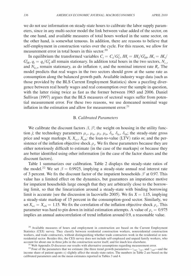
Table 1 summarizes our calibration. Table 2 displays the steady-state ratios of the model.22 We set β = 0.9925, implying a steady-state annual real interest rate of 3 percent. We fix the discount factor of the impatient households β′ at 0.97. This value has a limited effect on the dynamics, but guarantees an impatience motive for impatient households large enough that they are arbitrarily close to the borrow-ing limit, so that the linearization around a steady-state with binding borrowing limit is accurate (see the discussion in Iacoviello 2005). We fix X = 1.15, implying a steady-state markup of 15 percent in the consumption-good sector. Similarly, we set Xwc = Xwh = 1.15. We fix the correlation of the inflation objective shock ρs . This parameter was hard to pin down in initial estimation attempts. A value of ρs = 0.975 implies an annual autocorrelation of trend inflation around 0.9, a reasonable value.
20 Available measures of hours and employment in construction are based on the Current Employment Statistics (CES) survey. They classify between residential construction workers, nonresidential construction workers, and trade contractors, without distinguishing whether trade contractors work in the residential or non-residential sector. Besides this, the CES survey does not include self-employed and unpaid family workers, who account for about one in three jobs in the construction sector itself, and for much less elsewhere.
21 Web Appendix D discusses our results with alternative assumptions regarding measurement error.22 Four of the parameters that we estimate (the three trend growth parameters—γAk, γAc, and γAh—and the
income share of patient agents α) slightly affect the steady-state ratios. The numbers in Table 2 are based on the calibrated parameters and on the mean estimates reported in Tables 3 and 4.
VOL. 2 nO. 2 137iAcOViELLO And nEri: hOUSing MArkEt SpiLLOVErS
The depreciation rates for hous-ing, capital in the consumption sector, and capital in the housing sector are set equal to δh = 0.01, δkc = 0.025, and δkh = 0.03, respectively. The first number (together with j, the weight on housing in the utility function) pins down the ratio of residential invest-ment to total output at about 6 percent, as in the data. The other numbers, together with the capital shares in pro-duction, imply a ratio of nonresidential investment to GDP of about 27 percent. We pick a slightly higher value for the depreciation rate of construction capi-tal on the basis of BLS data on service lives of various capital inputs, which indicate that construction machinery (the data counterpart to kh) has a lower service life than other types of nonresidential equipment (the counterpart to kc).
For the capital share in the goods production function, we choose μc = 0.35. In the housing production function, we choose a capital share of μh = 0.10 and a land share of μl = 0.10, following Davis and Heathcote (2005). Together with the other estimated parameters, the chosen land share implies that the value of residential land is about 50 percent of annual GDP. This happens because the price of land capital-izes future housing production opportunities.23
We set the intermediate goods share at μb = 0.10. Input-output tables indicate a share of material costs for most sectors of around 50 percent, which suggests a cali-bration for μb as high as 0.50. We choose to be conservative because our value for μb is only meant to capture the extent to which sticky-price intermediate inputs are used in housing production. The weight on housing in the utility function is set at j = 0.12. Together with the technology parameters, these choices imply a ratio of business capital to annual GDP of about 2.1 and a ratio of housing wealth to GDP of about 1.35.
Next, we set the LTV ratio m. This parameter is difficult to estimate without data on debt and housing holdings of credit-constrained households. Our calibration is meant to measure the typical LTV ratio for homebuyers who are likely to be credit constrained and borrow the maximum possible against their home. Between 1973 and 2006, the average LTV ratio was 0.76.24 Yet “impatient” households might want to borrow more as a fraction of their home. In 2004, for instance, 27 percent of new home buyers took LTV ratios in excess of 80 percent, with an average ratio ( conditional on borrowing
23 Simple algebra shows that the steady-state value of land relative to residential investment equals ( pl/qih)= μl (βgc)/(1 − βgc). In practice, ownership of land entitles the household to the present discounted value of future income from renting land to housing production firms, which is proportional to μl. For μl = 0.10, β = 0.9925, qih/gdp = 0.06 and our median estimate of gc = 1.0047, this yields the value reported in the main text.
24 The data are from the Finance Board’s Monthly Survey of Rates and Terms on Conventional Single-Family Non-farm Mortgage Loans (summary table 19).
Table 1—Calibrated Parameters
Parameter Value
β 0.9925
β′ 0.97
j 0.12
μc 0.35
μh 0.10
μl 0.10
μb 0.10
δh 0.01
δkc 0.025
δkh 0.03
X, Xwc, Xwh 1.15
m 0.85
ρs 0.975

138 AMEricAn EcOnOMic JOUrnAL: MAcrOEcOnOMicS ApriL 2010
more than 80 percent) of 0.94. We choose to be conservative and set m = 0.85. It is conceivable that the assumption of a constant value for m over a 40-year period might be too strong, in light of the observation that the mortgage market has become more liberalized over time. We take these considerations into account when we estimate our model across subsamples, calibrating m differently across subperiods.
C. prior distributions
Our priors are in Tables 3 and 4. Overall, they are consistent with previous studies. We use inverse gamma priors for the standard errors of the shocks. For the persistence, we choose a beta-distribution with a prior mean of 0.8 and standard deviation of 0.1. We set the prior mean of the habit parameters in consumption (ε and ε′) at 0.5. For the monetary policy rule, we base our priors on a Taylor rule responding gradually to inflation only, so that the prior means of rr, rπ , and rY are, respectively, 0.75, 1.5, and 0. We set a prior on the capital adjustment costs of around 10.25 We choose a loose beta prior for the utilization parameter (ζ) between zero (capacity utilization can be varied at no cost) and one (capacity utilization never changes). For the disutility of working, we center the elasticity of the hours aggregator at 2 (the prior mean for η and η′ is 0.5). We select values for ξ and ξ′, the parameters describing the inverse elasticity of substitution across hours in the two sectors, of around one, as estimated by Horvath (2000). We select the prior mean of the Calvo price and wage parameter θπ , θwc , and θwh at 0.667, with a standard deviation of 0.05, values that are close to the estimates of Christiano, Eichenbaum, and Evans (2005). The priors for the indexation parameters ιπ , ι wc , and ιwh are loosely centered around 0.5, as in Smets and Wouters (2007).
We set the prior mean for the labor income share of unconstrained agents to be 0.65, with a standard error of 0.05. The mean is in the range of comparable estimates in the literature: for instance, using the 1983 Survey of Consumer Finances, Tullio Jappelli (1990) estimates 20 percent of the population to be liquidity constrained. Iacoviello (2005), using a limited information approach, estimates a wage share of collateral-constrained agents of 36 percent.
25 Given our adjustment cost specification (see Appendix B), the implied elasticity of investment to its shadow value is 1/(ϕδ). Our prior implies an elasticity of investment to its shadow price of about four.
Table 2—Steady-state Ratios
Variable Interpretation Value
4 × r − 1 Annual real interest rate 3%c/gdp Consumption share 67%ik/gdp Business investment share 27%q × ih/gdp Housing investment share 6%
qh/(4 × gdp) Housing wealth 1.36kc/(4 × gdp) Business capital in nonhousing sector 2.05kh/(4 × gdp) Business capital in housing sector 0.04pl/(4 × gdp) Value of land 0.50
note: Our model definition of GDP and consumption excludes the imputed value of rents from non-durable consumption.

VOL. 2 nO. 2 139iAcOViELLO And nEri: hOUSing MArkEt SpiLLOVErS
D. posterior distributions
Tables 3 and 4 report the posterior mean, median, and 95 probability intervals for the structural parameters, together with the mean and standard deviation of the prior distributions. In addition to the structural parameters, we estimate the standard devi-ation of the measurement error for hours and wage inflation in the housing sector.26
26 Draws from the posterior distribution of the parameters are obtained using the random walk version of the Metropolis algorithm. Tables and figures are based on a sample of 500,000 draws. The jump distribution was
Table 3—Prior and Posterior Distribution of the Structural Parameters
Prior distribution Posterior distribution
Parameter Distribution Mean SD Mean 2.5% Median 97.5%
ε Beta 0.5 0.075 0.32 0.25 0.33 0.40ε′ Beta 0.5 0.075 0.58 0.46 0.58 0.68η Gamma 0.5 0.1 0.52 0.34 0.52 0.75η′ Gamma 0.5 0.1 0.51 0.33 0.50 0.70ξ Normal 1 0.1 0.66 0.35 0.66 0.94ξ′ Normal 1 0.1 0.97 0.78 0.97 1.19ϕk,c Gamma 10 2.5 14.25 11.50 14.21 17.15ϕk,h Gamma 10 2.5 10.90 6.99 10.74 15.76α Beta 0.65 0.05 0.79 0.72 0.79 0.85rr Beta 0.75 0.1 0.59 0.50 0.59 0.67rπ Normal 1.5 0.1 1.44 1.33 1.44 1.55rY Normal 0 0.1 0.52 0.40 0.52 0.64θπ Beta 0.667 0.05 0.83 0.80 0.84 0.87ιπ Beta 0.5 0.2 0.69 0.52 0.68 0.87θw,c Beta 0.667 0.05 0.79 0.75 0.79 0.83ιw,c Beta 0.5 0.2 0.08 0.02 0.08 0.17θw,h Beta 0.667 0.05 0.91 0.87 0.91 0.93ιw,h Beta 0.5 0.2 0.40 0.17 0.40 0.63ζ Beta 0.5 0.2 0.69 0.46 0.69 0.87100γAc Normal 0.5 1 0.32 0.30 0.33 0.34100γAh Normal 0.5 1 0.08 −0.04 0.08 0.21100γAk Normal 0.5 1 0.27 0.24 0.26 0.29
Table 4—Prior and Posterior Distribution of the Shock Processes
Prior distribution Posterior distribution
Parameter Distribution Mean SD Mean 2.5% Median 97.5%
ρAc Beta 0.8 0.1 0.95 0.91 0.95 0.97ρAh Beta 0.8 0.1 0.997 0.993 0.997 0.999ρAk Beta 0.8 0.1 0.92 0.89 0.92 0.95ρj Beta 0.8 0.1 0.96 0.92 0.96 0.98ρz Beta 0.8 0.1 0.96 0.92 0.97 0.98ρτ Beta 0.8 0.1 0.92 0.87 0.92 0.96σAc Inv.gamma 0.001 0.01 0.0100 0.0090 0.0100 0.0111σAh Inv.gamma 0.001 0.01 0.0193 0.0173 0.0193 0.0214σAk Inv.gamma 0.001 0.01 0.0104 0.0082 0.0104 0.0129σj Inv.gamma 0.001 0.01 0.0416 0.0262 0.0413 0.0581σr Inv.gamma 0.001 0.01 0.0034 0.0029 0.0034 0.0042σz Inv.gamma 0.001 0.01 0.0178 0.0115 0.0172 0.0267στ Inv.gamma 0.001 0.01 0.0254 0.0188 0.0249 0.0339σp Inv.gamma 0.001 0.01 0.0046 0.0039 0.0046 0.0055σs Inv.gamma 0.001 0.01 0.0004 0.0003 0.0004 0.0005σn,h Inv.gamma 0.001 0.01 0.1218 0.1079 0.1216 0.1361σw,h Inv.gamma 0.001 0.01 0.0071 0.0063 0.0070 0.0080

140 AMEricAn EcOnOMic JOUrnAL: MAcrOEcOnOMicS ApriL 2010
We find a faster rate of technological progress in business investment, followed by consumption and by the housing sector. In the next section, we discuss the implica-tions of these findings for the long-run properties of consumption, housing invest-ment, and real house prices.
One key parameter relates to the labor income share of credit-constrained agents. Our estimate of α is 0.79. This number implies a share of labor income accruing to credit-constrained agents of 21 percent. This value is lower than our prior mean. However, as we document below, this value is large enough to generate a positive elasticity of consumption to house prices after a housing demand shock (see the next section).27
Both agents exhibit a moderate degree of habit formation in consumption and relatively little preference for mobility across sectors, as shown by the positive val-ues of ξ and ξ′. The degree of habits in consumption is larger for the impatient house-holds than for patient ones (ε′ = 0.58 and ε = 0.32). One explanation may be that since impatient households do not hold capital, and they cannot smooth consumption through saving, a larger degree of habits is needed in order to match the persistence of aggregate consumption in the data. Turning to the labor supply elasticity, the posterior distributions of η and η′ (centered around 0.50) show that the data do not convey much information on these parameters. We performed sensitivity analysis with respect to these parameters and found that the main results are not particularly sensitive for a reasonable range of values of η and η′.
The estimate of θπ (0.83) implies that prices are reoptimized once every six quar-ters. However, given the positive indexation coefficient (ιπ = 0.69), prices change every period, although not in response to changes in marginal costs. As for wages, we find that stickiness in the housing sector (θwh = 0.91) is higher than in the con-sumption sector (θwc = 0.79), while wage indexation is larger in housing (ιwh = 0.40 and ιwc = 0.08).
Estimates of the monetary policy rule are in line with previous evidence. Finally, all shocks are quite persistent, with autocorrelation coefficients ranging between 0.92 and 0.997.
III. Properties of the Estimated Model
A. impulse responses
housing preference Shock.—Figure 2 plots impulse responses to the estimated housing preference shock. We also call this shock a housing demand shock, since it raises house prices and the returns to housing investment, thus causing the latter to rise. The shock also increases the collateral capacity of constrained agents, thus
chosen to be the normal one with covariance matrix equal to the Hessian of the posterior density evaluated at the maximum. The scale factor was chosen in order to deliver an acceptance rate of about 25 percent. Convergence was assessed by comparing the moments computed by splitting the draws of the Metropolis into two halves. See Web Appendix C for more details.
27 Impatient households have a higher marginal propensity to consume (because of their low discount fac-tor), but a low average propensity to consume (because of the high steady state debt payments). Because of this, despite their 21 percent wage share, they account for 17 percent of total consumption and own 14 percent of the total housing stock.

VOL. 2 nO. 2 141iAcOViELLO And nEri: hOUSing MArkEt SpiLLOVErS
allowing them to increase borrowing and consumption. Since borrowers have a high marginal propensity to consume, the effects on total consumption are positive, even if consumption of the lenders (not plotted) falls.
An interesting property of the estimated shock is that it generates a long lasting increase in house prices. The strong persistence of house prices reflects the dynamic process that characterizes the preference shock process, for which estimated auto-correlation is 0.96, rather than the intrinsic dynamics of the house price process which, as the two housing demand equations show, are forward looking (see equa-tions (B2) and (B14) in the Appendix B).
Figure 2 also displays the responses for three alternative versions of the model in which we set θp = 0 (flexible prices), θwc = θwh =0 (flexible wages), and α = 1 (no collateral effects), while holding the remaining parameters at the benchmark val-ues. As the figure illustrates, collateral effects are the key feature of the model that generates a positive and persistent response of consumption following an increase in housing demand. Absent this effect, in fact, an increase in the demand for
0 5 10 15 20−0.05
0
0.05
0.1Real consumption
0 5 10 15 20−0. 2
−0. 1
0
0.1
0.2Real business investment
0 5 10 15 200
1
2
3
4Real residential investment
0 5 10 15 200.2
0.4
0.6
0.8
1Real house prices
0 5 10 15 200
0.1
0.2
0.3Real GDP
0 5 10 15 200
0.02
0.04
0.06Nominal interest rate
Baseline
Flexible price
Flexible wage
No collateral effect
Figure 2. Impulse Responses to a Housing Preference Shock: Baseline Estimates and Sensitivity Analysis
note: The y-axis measures percent deviation from the steady state.

142 AMEricAn EcOnOMic JOUrnAL: MAcrOEcOnOMicS ApriL 2010
housing would generate an increase in housing investment and housing prices, but a fall in consumption. Quantitatively, the observed impulse response translates into a first-year elasticity of consumption to housing prices (conditional on the shock) of around 0.07. This result mirrors the findings of several papers that document posi-tive effects on consumption from changes in housing wealth (see, for instance, Karl E. Case, John M. Quigley, and Robert J. Shiller 2005; and John Y. Campbell and Joao F. Cocco 2007). It is tempting to compare our results with theirs. However, our elasticity is conditional to a particular shock, whereas most microeconometric and time-series studies in the literature try to isolate the elasticity of consumption to housing prices through regressions of consumption on housing wealth, both of which are endogenous variables in our model. We return to this issue in the next section.
Next, we consider the response of residential investment. At the baseline esti-mates, a shift in housing demand that generates an increase in real house prices of about 1 percent (see Figure 2) causes residential investment to rise by about 3.5 per-cent. As the figure illustrates, sticky wages are crucial here. In particular, the combi-nation of flexible housing prices and sticky wages in construction makes residential investment very sensitive to changes in demand conditions. The numbers can be related to the findings of Robert H. Topel and Sherwin Rosen (1988), who estimate an elastic response of new housing supply to changes in prices. For every 1 percent increase in house prices lasting for two years, they find that new construction rises on impact between 1.5 and 3.15 percent, depending on the specifications.
Finally, we consider business investment. The impulse response of business investment is the combined effect of two forces. On the one hand, capital in the construction sector kh rises. On the other hand, there is slow and persistent decline in capital in the consumption sector kc, which occurs since resources are shifted away from one sector to the other. The two effects roughly offset each other, and the overall response of business investment is small.
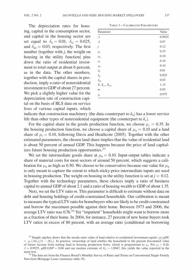
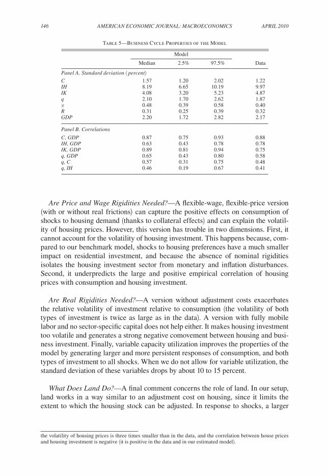
Monetary Shock.—Figure 3 plots an adverse independent and identically distrib-uted monetary policy shock. Real house prices drop and remain below the base-line for about six quarters. The quantitative effect of the monetary shock on house prices is similar to what is found in VAR studies of the impact of monetary shocks on house prices (see, for instance, Iacoviello 2005). All components of aggregate demand fall, with housing investment showing the largest drop, followed by business investment and consumption. The large drop in housing investment is a well-docu-mented fact in VAR studies (e.g., Ben S. Bernanke and Mark Gertler 1995). As the figure shows, both nominal rigidities and collateral effects amplify the response of consumption to monetary shocks. Instead, the responses of both types of investment are only marginally affected by the presence of collateral constraints. The reason for this result is, in our opinion, that the model ignores financing frictions on the side of the firms. In fact, collateral effects slightly reduce the sensitivity of investment to monetary shocks, since unconstrained households shift loanable funds from the con-strained households toward firms in order to smooth their consumption. Finally, the negative response of real house prices to monetary shocks, instead, mainly reflects nominal stickiness.
VOL. 2 nO. 2 143iAcOViELLO And nEri: hOUSing MArkEt SpiLLOVErS
The response of residential investment is five times larger than consumption and twice as large as business investment. As Figure 3 shows, wage rigidity is instrumental for this result. Housing investment is interest rate sensitive only when wage rigidity is present.28 In particular, housing investment falls because housing prices fall relative to wages. Housing investment falls a lot because the flow of housing investment is small relative to its stock, so that the drop in investment has to be large to restore the desired stock-flow ratio. Our results support the findings of Barsky, House, and Kimball (2007) and Charles T. Carlstrom and Timothy S. Fuerst (2006), who show how models with rigid nondurable prices and flexible durable
28 In robustness experiments, we have found that sectoral wage rigidity (rather than overall wage rigidity) matters for this result. That is, sticky wages in the housing sector, and flexible wages in the nonhousing sector, are already sufficient to generate a large response of residential investment to monetary shocks.
0 5 10 15 20
−0. 4
−0. 2
0
Real consumption
0 5 10 15 20−1. 5
−1
−0. 5
0
0.5
Real business investment
0 5 10 15 20−4
−2
0
2
Real residential investment
0 5 10 15 20−1
−0. 5
0
0.5
Real house prices
0 5 10 15 20−1
−0. 5
0
0.5
Real GDP
0 5 10 15 20−0.05
0
0.05
0.1
0.15
Nominal interest rate
Baseline
Flexible price
Flexible wage
No collateral effect
Figure 3. Impulse Responses to an Independently and Identically Distributed Monetary Policy Shock: Baseline Estimates and Sensitivity Analysis
note: The y-axis measures percent deviation from the steady state.

144 AMEricAn EcOnOMic JOUrnAL: MAcrOEcOnOMicS ApriL 2010
prices may generate a puzzling increase in durables following a negative monetary shock, and that sticky wages can eliminate this puzzle.29
housing technology and Other Shocks.—Positive technology shocks in the hous-ing sector (plotted in Figure 4) lead to a rise in housing investment and, thanks to a fall in construction costs, to a drop in housing prices. As for the responses of aggregate variables to other shocks, our findings resemble those of estimated DSGE models that do not include a housing sector (e.g., Smets and Wouters 2007, and Alejandro Justiniano, Giorgio Primiceri, and Andrea Tambalotti 2009). In par-ticular, positive technology shocks in the nonhousing sector drive up both housing investment and housing prices; temporary cost-push shocks lead to an increase in inflation and a decline in house prices, and persistent shifts in the inflation target persistently move up both inflation and housing prices.
B. cyclical properties
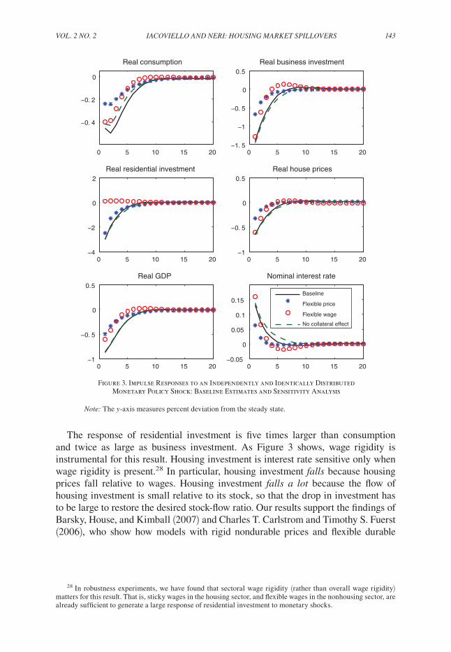
Our estimated model explains the behavior of housing and nonhousing variables well. As Table 5 shows, most of the model’s business cycle statistics are within the 95 percent probability interval computed from the data.30 The model replicates well the joint behavior of the components of aggregate demand, the cyclicality and vola-tility of housing prices, and the patterns of comovement between housing and non-housing variables.31
C. robustness Analysis
The ability of the model to match volatilities and correlations that are found in the data is, of course, the outcome of having several shocks and frictions. The introduction of a large number of them, while common in the literature on estimated DSGE models, raises the question as to which role each of them plays. Below, we summarize our main findings. We do so by reporting the main properties of our
29 A natural question to ask is the extent to which one can regard construction as a sector featuring strong wage rigidities. There is evidence in this regard. First, construction has higher unionization rates relative to the private sector: 15.4 percent versus 8.6 percent. Second, several state and federal wage laws in the construction industry insulate movements in wages from movements in the marginal cost of working. The Davis-Bacon Act, for instance, is a federal law mandating a prevailing wage standard in publicly funded construction projects; sev-eral states have followed with their own wage legislation, and the provisions of the Davis-Bacon Act also apply to private construction firms.
30 The statistics are computed using a random selection of 1,000 draws from the posterior distribution and, for each of them, 100 artificial time series of the main variables of length equal to that of the data, giving a sample of 100,000 series. The business cycle component of each simulated series is extracted using the HP filter (with smoothing parameter set to 1,600). Summary statistics of the posterior distribution of the moments are computed by pooling together all the simulations. GDP denotes domestic demand excluding government purchases and investment, chained 2000 dollars.
31 In our estimated model, the peak correlation of housing investment with other components of aggregate demand (consumption and business investment) is the contemporaneous one. In the data, housing investment comoves with consumption, but leads business investment by two quarters. Fisher (2007) develops a model that extends the home production framework to make housing complementary to labor and capital in business produc-tion. He shows that in such a model housing investment leads business investment.

VOL. 2 nO. 2 145iAcOViELLO And nEri: hOUSing MArkEt SpiLLOVErS
model shutting off once at the time selected shocks or frictions, and holding all other parameters at their estimated value.32
can technology Shocks Account for the Main properties of the data?—A model with only technology shocks, keeping nominal and real rigidities, explains only half of the volatility of housing prices and housing investment. In addition, it gener-ates (contrary to the data) a negative correlation between house prices and housing investment, mostly because housing technology shocks are needed to account for the volatility of housing investment, but these shocks move the price and the quantity of housing in opposite directions.33
32 In Web Appendix D, we report the results of the sensitivity analysis after shutting off shocks and/or fric-tions and reestimating all the other parameters. The results were qualitatively and quantitatively the same.
33 The inability of a model with only technology shocks to explain housing prices and housing investment is in line with the findings of Davis and Heathcote (2005). In their model (which is driven by technology shocks only),
0 5 10 15 20−0.15
−0. 1
−0.05
0
0.05Real consumption
0 5 10 15 20−0. 2
−0. 1
0
0.1
0.2Real business investment
0 5 10 15 201
2
3
4Real residential investment
0 5 10 15 20−0. 9
−0. 8
−0. 7
−0. 6
−0. 5Real house prices
0 5 10 15 200.05
0.1
0.15
0.2
0.25Real GDP
0 5 10 15 20−0.05
0
0.05
0.1
0.15
Nominal interest rate
Baseline
Flexible price
Flexible wage
No collateral effects
Figure 4. Impulse Responses to a Housing Technology Shock: Baseline Estimates and Sensitivity Analysis
note: The y-axis measures percent deviation from the steady state.
146 AMEricAn EcOnOMic JOUrnAL: MAcrOEcOnOMicS ApriL 2010
Are price and Wage rigidities needed?—A flexible-wage, flexible-price version (with or without real frictions) can capture the positive effects on consumption of shocks to housing demand (thanks to collateral effects) and can explain the volatil-ity of housing prices. However, this version has trouble in two dimensions. First, it cannot account for the volatility of housing investment. This happens because, com-pared to our benchmark model, shocks to housing preferences have a much smaller impact on residential investment, and because the absence of nominal rigidities isolates the housing investment sector from monetary and inflation disturbances. Second, it underpredicts the large and positive empirical correlation of housing prices with consumption and housing investment.
Are real rigidities needed?—A version without adjustment costs exacerbates the relative volatility of investment relative to consumption (the volatility of both types of investment is twice as large as in the data). A version with fully mobile labor and no sector-specific capital does not help either. It makes housing investment too volatile and generates a strong negative comovement between housing and busi-ness investment. Finally, variable capacity utilization improves the properties of the model by generating larger and more persistent responses of consumption, and both types of investment to all shocks. When we do not allow for variable utilization, the standard deviation of these variables drops by about 10 to 15 percent.
What does Land do?—A final comment concerns the role of land. In our setup, land works in a way similar to an adjustment cost on housing, since it limits the extent to which the housing stock can be adjusted. In response to shocks, a larger
the volatility of housing prices is three times smaller than in the data, and the correlation between house prices and housing investment is negative (it is positive in the data and in our estimated model).
Table 5—Business Cycle Properties of the Model
Model
Median 2.5% 97.5% Data
panel A. Standard deviation ( percent)c 1.57 1.20 2.02 1.22ih 8.19 6.65 10.19 9.97ik 4.08 3.20 5.23 4.87q 2.10 1.70 2.62 1.87π 0.48 0.39 0.58 0.40r 0.31 0.25 0.39 0.32gdp 2.20 1.72 2.82 2.17
panel B. correlations
c, gdp 0.87 0.75 0.93 0.88ih, gdp 0.63 0.43 0.78 0.78ik, gdp 0.89 0.81 0.94 0.75q, gdp 0.65 0.43 0.80 0.58q, c 0.57 0.31 0.75 0.48q, ih 0.46 0.19 0.67 0.41

VOL. 2 nO. 2 147iAcOViELLO And nEri: hOUSing MArkEt SpiLLOVErS
land share reduces the volatility of housing investment and increases the volatility of prices.
Are the results Sensitive to the Use of Alternative house price Measures?—As a robustness check, we have estimated our model using the OFHEO index as a mea-sure of house prices, and using both the census and the OFHEO index under the assumption that each of them measures house prices up to some measurement error. Web Appendix D reports our results in detail. Our main findings (in terms of param-eters estimates, impulse responses, and historical decompositions) were qualitatively and quantitatively unaffected. We conjecture that this result occurs because the main differences between the two series stem more from their low-frequency component than from their cyclical properties. The main difference across parameter estimates is that using the OFHEO series lowers the estimated coefficient on trend growth in housing technology, since the OFHEO series exhibits a stronger upward trend over the sample period.
Are the results Sensitive to the Assumption of heterogeneous preferences?—In our baseline model, we have allowed habits and labor supply parameters to differ across agents. Web Appendix D reports the results when we constrain ε, η, and ξ to be the same across patient and impatient agents. The results are essentially unchanged. The model with common preference parameters, if anything, displays a larger response of consumption (and smaller response of housing investment) to a housing preference shock.
IV. Sources and Consequences of Housing Market Fluctuations
Having shown that the estimated model fits the data reasonably well, we use it to address the two questions we raised at the start of this paper. First, what are the main driving forces of fluctuations in the housing market? Second, how large are the spillovers from the housing market to the broader economy?
A. What drives the housing Market?
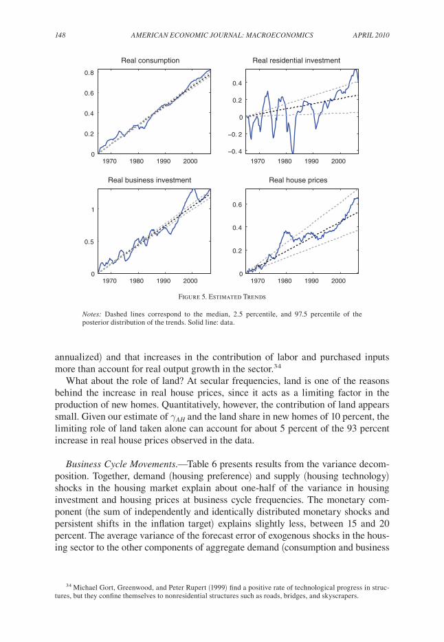
trend Movements.—We find a faster rate of technological progress in business investment, followed by the consumption sector and, last, by the housing sector. At the posterior median, the long-run quarterly growth rates of consumption, hous-ing investment, and real house prices (as implied by the values of the γ terms and equations (12)–(15)) are, respectively, 0.47, 0.15, and 0.32 percent. In other words, the trend rise in real house prices observed in the data reflects, according to our estimated model, faster technological progress in the nonhousing sector. As shown in Figure 5, our estimated trends fit the secular behavior of consumption, investment and house prices well. According to the model, the slow rate of increase of produc-tivity in construction is behind the secular increase in house prices. Our finding is in line with the results of Carol Corrado et al. (2006), who construct sectoral mea-sures of Total Factor Productivity (TFP) growth for the United States. They also find that the average TFP growth in the construction sector is negative (−0.5 percent,
148 AMEricAn EcOnOMic JOUrnAL: MAcrOEcOnOMicS ApriL 2010
annualized) and that increases in the contribution of labor and purchased inputs more than account for real output growth in the sector.34
What about the role of land? At secular frequencies, land is one of the reasons behind the increase in real house prices, since it acts as a limiting factor in the production of new homes. Quantitatively, however, the contribution of land appears small. Given our estimate of γAh and the land share in new homes of 10 percent, the limiting role of land taken alone can account for about 5 percent of the 93 percent increase in real house prices observed in the data.
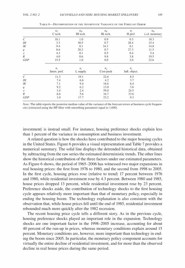
Business cycle Movements.—Table 6 presents results from the variance decom-position. Together, demand (housing preference) and supply (housing technology) shocks in the housing market explain about one-half of the variance in housing investment and housing prices at business cycle frequencies. The monetary com-ponent (the sum of independently and identically distributed monetary shocks and persistent shifts in the inflation target) explains slightly less, between 15 and 20 percent. The average variance of the forecast error of exogenous shocks in the hous-ing sector to the other components of aggregate demand (consumption and business
34 Michael Gort, Greenwood, and Peter Rupert (1999) find a positive rate of technological progress in struc-tures, but they confine themselves to nonresidential structures such as roads, bridges, and skyscrapers.
1970 1980 1990 20000
0.2
0.4
0.6
0.8
Real consumption
1970 1980 1990 2000
−0. 4
−0. 2
0
0.2
0.4
Real residential investment
1970 1980 1990 20000
0.5
1
Real business investment
1970 1980 1990 20000
0.2
0.4
0.6
Real house prices
Figure 5. Estimated Trends
notes: Dashed lines correspond to the median, 2.5 percentile, and 97.5 percentile of the posterior distribution of the trends. Solid line: data.
VOL. 2 nO. 2 149iAcOViELLO And nEri: hOUSing MArkEt SpiLLOVErS
investment) is instead small. For instance, housing preference shocks explain less than 1 percent of the variance in consumption and business investment.
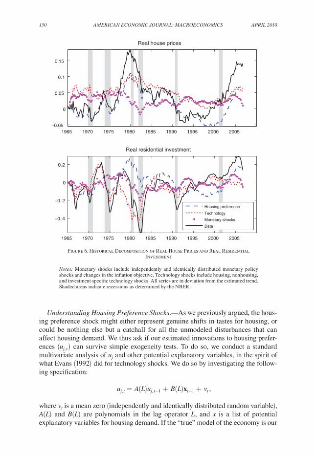
A related question is how the shocks have contributed to the major housing cycles in the United States. Figure 6 provides a visual representation and Table 7 provides a numerical summary. The solid line displays the detrended historical data, obtained by subtracting from the raw series the estimated deterministic trends. The other lines show the historical contribution of the three factors under our estimated parameters. As Figure 6 shows, the period of 1965–2006 has witnessed two major expansions in real housing prices: the first from 1976 to 1980, and the second from 1998 to 2005. In the first cycle, housing prices rose (relative to trend) 17 percent between 1976 and 1980, while residential investment rose by 4.3 percent. Between 1980 and 1985, house prices dropped 13 percent, while residential investment rose by 23 percent. Preference shocks aside, the contribution of technology shocks to the first housing cycle appears relatively more important than that of monetary policy, especially in ending the housing boom. The technology explanation is also consistent with the observation that, while house prices fell until the end of 1985, residential investment rebounded much more quickly after the 1982 recession.
The recent housing price cycle tells a different story. As in the previous cycle, housing preference shocks played an important role in the expansion. Technology shocks are one important factor in the 1998–2005 increase, accounting for about 40 percent of the run-up in prices, whereas monetary conditions explain around 15 percent. Monetary conditions are, however, more important than technology in end-ing the boom since 2005. In particular, the monetary policy component accounts for virtually the entire decline of residential investment, and for more than the observed decline in real house prices during the same period.
Table 6—Decomposition of the Asymptotic Variance of the Forecast Error
uc uh uk uj ur C tech. IH tech. IK tech. H pref. i.i.d. monetary
c 18.1 1.0 0.9 0.3 18.3ih 3.3 30.5 0.7 28.4 15.4ik 9.4 0.1 34.3 0.1 14.8q 8.6 20.2 0.7 27.3 11.5π 4.3 0.1 0.5 0.4 5.4r 4.0 0.6 9.8 3.8 19.5gdp 15.5 1.0 8.0 2.0 22.6
uz uτ up us Intert. pref. L supply Cost-push Infl. object.
c 11.3 19.1 22.6 8.5ih 7.4 6.6 4.2 3.7ik 7.1 9.4 18.6 6.4q 9.2 6.2 13.0 3.6π 3.4 2.4 59.0 24.5r 6.6 5.6 16.7 33.6gdp 1.0 17.7 23.2 9.3
note: The table reports the posterior median value of the variance of the forecast errors at business cycle frequen-cies (extracted using the HP filter with smoothing parameter equal to 1,600).
150 AMEricAn EcOnOMic JOUrnAL: MAcrOEcOnOMicS ApriL 2010
Understanding housing preference Shocks.—As we previously argued, the hous-ing preference shock might either represent genuine shifts in tastes for housing, or could be nothing else but a catchall for all the unmodeled disturbances that can affect housing demand. We thus ask if our estimated innovations to housing prefer-ences (uj, t ) can survive simple exogeneity tests. To do so, we conduct a standard multivariate analysis of uj and other potential explanatory variables, in the spirit of what Evans (1992) did for technology shocks. We do so by investigating the follow-ing specification:
uj, t = A(L)uj, t−1 + B(L)xt−1 + vt ,
where vt is a mean zero (independently and identically distributed random variable), A(L) and B(L) are polynomials in the lag operator L, and x is a list of potential explanatory variables for housing demand. If the “true” model of the economy is our
1965 1970 1975 1980 1985 1990 1995 2000 2005−0.05
0
0.05
0.1
0.15
Real house prices
1965 1970 1975 1980 1985 1990 1995 2000 2005
−0. 4
−0. 2
0
0.2
Real residential investment
Housing preference
Technology
Monetary shocks
Data
Figure 6. Historical Decomposition of Real House Prices and Real Residential Investment
notes: Monetary shocks include independently and identically distributed monetary policy shocks and changes in the inflation objective. Technology shocks include housing, nonhousing, and investment specific technology shocks. All series are in deviation from the estimated trend. Shaded areas indicate recessions as determined by the NBER.

VOL. 2 nO. 2 151iAcOViELLO And nEri: hOUSing MArkEt SpiLLOVErS
DSGE model, no variable should cause (in the sense of Granger) the innovations to housing preferences. A more mundane interpretation is that the shock could capture shifters of housing demand that are not explicitly included in our stylized model. The question is: what are these shifters, and do they affect housing demand in an economically reasonable way?
The typical determinants of housing demand that the literature has looked at include the number of potential housing consumers, their financial resources and tastes, and measures of the user cost of housing that account for deductability of mortgage interest payment. Some of these determinants have already been included in our model. We follow a flexible approach and include numerous controls in the list of regressors. These regressors are: Initial Fees and Charges for a Mortgage (iFAc, measured in percent of the loan), Civilian Labor Force (cLF ), Household leverage (LEV, constructed as the ratio of outstanding home mortgages to holdings of residen-tial real estate), the University of Michigan Index of Consumer Sentiment (cS ), the share of population between ages 25 and 39 (pOp2539 ),35 and the share of subprime mortgages in total mortgage originations (SUBpriME ).36 In addition, we also add inflation (inFL, constructed as in Section II) and the real after-tax mortgage rate (rtAX ). If inflation illusion matters for house prices, one should expect an effect of inflation on house prices over and above the conventional effects of inflation on housing demand that our DSGE model should capture. The real after-tax mortgage rate is constructed as 0.7rM–inFL, where rM is the 30-year conventional mortgage rate, and the tax rate is set at 30 percent. If deductability of mortgage payments
35 We convert the original annual series into a quarterly series assuming that the underlying series follows an ARIMA(1,1,0) process with autoregressive coefficient equal to 0.99.
36 The subprime market was virtually nonexistent prior to 1995. The share of subprime mortgages in total mortgage originations was 1.5 percent in 1994, 8 percent in 2003, and peaked at 20 percent in 2005. We set it equal to zero for all the periods prior to 1994. We convert the original annual series into a quarterly series assum-ing that the underlying series follows an ARIMA(1,1,0) process with autoregressive coefficient equal to 0.99.
Table 7—Contribution to Housing Booms of the Estimated Shocks
Percent change Contribution to changes of:
Period q Technology Monetary pol. Housing pref.
1976:QI 1980:QI 16.8 4.8 −3.0 11.41980:QII 1985:QIV −13.3 −4.0 −0.1 −6.3
1998:QI 2005:QI 13.9 5.4 2.1 9.32005:QII 2006:QIV −0.6 −0.3 −2.8 0.5
ih
1976:QI 1980:QI 4.3 −25.9 −11.4 31.41980:QII 1985:QIV 22.8 46.8 −2.2 −16.3
1998:QI 2005:QI 21.9 −3.3 10.8 27.12005:QII 2006:QIV −15.1 −3.2 −12.0 −4.2
notes: Contribution of technology shocks (nonhousing, housing, and investment specific), Monetary shocks (interest rate and inflation objective) and housing preference shocks to the housing market cycles reported in the text. Changes in the variables are expressed in deviation from the estimated trends.

152 AMEricAn EcOnOMic JOUrnAL: MAcrOEcOnOMicS ApriL 2010
matters, rM should have an effect on housing demand over and above the effect of real interest rates.37
In our baseline specification, we enter all variables, except inFL, in first dif-ferences (one lag was sufficient to obtain independently and identically distributed residuals). Table 8 presents our results. Some of the variables in the regressions are significant and have the expected sign, although their combined explanatory power is low (the r2 is about 15 percent). Our preferred specification keeps only the vari-ables that are significant at the 10 percent level in the initial regression. The prefer-ence shock depends negatively on initial fees and charges (low initial fees might lure people into buying more housing than otherwise needed). It depends negatively on inflation (thus going against the idea that higher inflation spurs housing demand over and above the effect that inflation has on economic activity). It depends positively on the share of population in the 25–39 years-old range; and it depends positively on the share of subprime mortgages.38 Figure 7 plots actual and fitted values from our preferred regression. Overall, the results provide some evidence that some of the model’s omitted variables capture part of the preference shock. For instance, the rise and the fall in the subprime mortgage market of the 2003–2006 period accounts for
37 Data sources are as follows. IFAC: Finance Board’s Monthly Survey of Rates and Terms on Conventional Single-Family Nonfarm Mortgage Loans, Table 17: Terms on Conventional Single-Family Mortgages, Monthly National Averages, All Homes; CLF: Bureau of Labor Statistics. LEV: Federal Reserve Board Flow of Funds Tables, constructed as ratio of outstanding home mortgages (series FL153165105.Q) over holdings of residential real estate (series FL155035015.Q); CS: Survey Research Center: University of Michigan. POP2539: US Census Bureau International Data Base. SUBPRIME: Inside Mortgage Finance. RTAX: constructed as 0.7rMt − πt , where RM is the 30-year conventional mortgage rate from the Board of Governors of the Federal Reserve System, H.15 Release.
38 Another potential candidate is homeownership. Homeownership rates in the United States were constant around 64/65 percent between 1970 and 1995, and rose at a constant pace up to 69 percent at the peak of the hous-ing boom in 2005. We found no explanatory power for this variable.
Table 8—Predictability of the Housing Preference Impulse
Significance levelx-vector t-statistic test h0 : B(L) = 0
(a) corrected r2 = 0.14
All variables below 0.0107 Δ IFAC(−1) −1.78 0.0743 Δ CLF(−1) 1.29 0.1978 Δ LEV(−1) −0.28 0.7778 Δ CS(−1) 0.79 0.4303 Δ POP2539(−1) 2.37 0.0179 Δ SUBPRIME(−1) 3.02 0.0025 INFL(−1) −1.80 0.0714 Δ RTAX(−1) −0.72 0.4701
(b) corrected r2 = 0.15
All variables below 0.0016 Δ IFAC(−1) −1.85 0.0637 Δ POP2539(−1) 2.74 0.0062 Δ SUBPRIME(−1) 2.81 0.0049 INFL(−1) −1.99 0.0462
notes: Predictability of our housing preference impulse uj,t = A(L)uj,t−1 + B(L)xt−1 + vt . One lag of uj,t and xt were chosen.
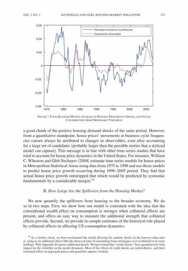
VOL. 2 nO. 2 153iAcOViELLO And nEri: hOUSing MArkEt SpiLLOVErS
a good chunk of the positive housing demand shocks of the same period. However, from a quantitative standpoint, house prices’ movements at business cycle frequen-cies cannot always be attributed to changes in observables, even after accounting for a large set of candidates (probably larger than the possible stories that a stylized model can capture). This message is in line with other time-series studies that have tried to account for house price dynamics in the United States. For instance, William C. Wheaton and Gleb Nechayev (2008) estimate time series models for house prices in Metropolitan Statistical Areas using data from 1975 to 1998 and use those models to predict house price growth occurring during 1998–2005 period. They find that actual house price growth outstripped that which would be predicted by economic fundamentals by a considerable margin.39
B. how Large Are the Spillovers from the housing Market?
We now quantify the spillovers from housing to the broader economy. We do so in two steps. First, we show how our model is consistent with the idea that the conventional wealth effect on consumption is stronger when collateral effects are present, and offers an easy way to measure the additional strength that collateral effects provide. Second, we provide in-sample estimates of the historical role played by collateral effects in affecting US consumption dynamics.
39 As a further check, we have reestimated the model allowing for random shocks in the loan-to-value ratio m, using as an additional observable the observed ratio of oustanding home mortgages over residential real estate holdings. Web Appendix D reports additional details. We have found that “credit shocks” have quantitatively little impact for the volatility on the model dynamics. Most of the effects of credit shocks are redistributive, and their estimated effect on aggregate prices and quantities appears limited.
1975 1980 1985 1990 1995 2000 2005−0.06
−0.04
−0.02
0
0.02
0.04
0.06
Estimated innovations to preferences
Explained by observables
Figure 7. Four-Quarter Moving Average of Housing Preference Shocks and Fitted Contribution from Observable Variables

154 AMEricAn EcOnOMic JOUrnAL: MAcrOEcOnOMicS ApriL 2010
the housing Wealth Effect.—As we explained above, a large part of the model spill-overs occur through the effects that fluctuations in housing prices have on consumption. These effects are reinforced by the degree of financial frictions, as measured by the wage share of credit constrained agents and by the loan-to-value ratio. To measure the spillovers, we run a basic regression that allows for changes in housing wealth to affect aggregate consumption. This equation can be interpreted as a reduced-form way of capturing the direct and indirect effects that fluctuations in housing wealth have on aggregate consumption, although both variables are endogenous in our model. In the simulated output of our model, regressing consumption growth on lagged growth in housing wealth yields (standard errors are in parenthesis):40
Δ ln ct = 0.0041 (0.0007)
+ 0.133 (0.043)
Δ ln hWt−1 .
The coefficients of the artificial regression are in the same ballpark as those from the analogous regression on actual data,41 which gives:
Δ ln ct = 0.0039 (0.0006)
+ 0.122 (0.039)
Δ ln hWt−1 .
Specifications of this kind have a long tradition in macroeconometric models, and our measured housing wealth effect from the data and the baseline model is in the ballpark of existing estimates (see the survey by James M. Poterba 2000). Needless to say, the positive number above captures, in the model as in the data, the influ-ence of common macroeconomic factors as well as the direct effect of changes in housing wealth on consumption through the collateral channel. However, an impor-tant advantage of our model relative to the data-based regressions is that the model allows disentangling the two effects. To do so, we run the same regression using the simulated model output in the absence of collateral effects (that is, setting α = 1). This regression yields a smaller coefficient on housing wealth, equal to 0.108. The comparison between the estimates with and without collateral effects offers a way to measure the spillovers from the housing market to consumption that work through the direct collateral effect. In practice, it suggests that collateral effects increase the elasticity of consumption to housing wealth by 2.5 percentage points (from 0.108 to 0.133).42
Is this effect large or small? Obviously, our equation is misspecified relative to the structural equilibrium relationships implied by our model. The correct relation-ship between consumption and housing wealth is part of the equilibrium law of
40 The model variables have been generated using the posterior median of the parameters and drawing shocks from their distribution. One thousand samples of observations of length equal to the data were generated. The numbers in the text are averages across all regressions. We experimented with specifications including lagged income, nonhousing wealth, and interest rates as controls. These variables turned out to be insignificant.
41 The housing wealth series is from the Flow of Funds (Balance sheet of households and nonprofit organiza-tions: B.100, row 4), and measures the market value of household real estate wealth (code FL155035015). The series is deflated with the nonfarm business sector deflator and normalized by civilian noninstitutional population.
42 When we condition on housing preference shocks only, the analogous regression coefficient is 0.028 when α equals its estimated value of 0.79, and falls to 0.011 when α is set equal to 1.

VOL. 2 nO. 2 155iAcOViELLO And nEri: hOUSing MArkEt SpiLLOVErS
motion of the model, which takes the form of a vector autoregressive moving aver-age process incorporating all the endogenous variables of the model. However, our model is consistent with the idea that the so-called wealth effect on consumption increases with the fraction of households who use their home as collateral.43 The other takeaway is that, even without collateral constraints, our model generates a positive comovement between changes in housing wealth and changes in future con-sumption. This comovement reflects the result that most of our identified shocks generate a positive correlation between housing wealth and consumption. When col-lateral effects are present, however, such correlation becomes larger. We can express the elasticity of consumption growth to housing wealth growth as the product of the correlation between the two variables, say ρ, times the ratio of their standard devia-tions. Collateral effects increase the elasticity because they reinforce the correlation between the two variables (when α goes from 1 to 0.79, the corresponding value of ρ rises from 0.19 to 0.23), while they affect the volatility of consumption growth and housing wealth growth little.
Subsample Estimates: Financial Liberalization and the historical contribution of collateral Effects.—In our baseline estimates, we have kept the assumption that the structural parameters were constant throughout the sample. However, several market innovations following the financial reforms of the early 1980s affected the housing market. Jeffrey R. Campbell and Hercowitz (2005), for instance, argue that mortgage market liberalization drastically reduced the equity requirements associ-ated with collateralized borrowing. More in general, several developments in the credit market might have enhanced the ability to households to borrow, thus reduc-ing the fraction of credit constrained households, as pointed out by Karen E. Dynan, Douglas W. Elmendorf, and Daniel Sichel (2006). Motivated by this evidence, we estimate our model across two subperiods, and use our estimates to measure the feed-back from housing market fluctuations to consumer spending. Following Campbell and Hercowitz (2005), we set a “low” loan-to-value ratio in the first subperiod and a “high” loan-to-value ratio in the second subperiod in order to model financial liberal-ization in our setup. Namely, we set m = 0.775 in the period 1965:QI–1982:QIV, and m = 0.925 in the period 1989:QI–2006:QIV.44 As we mentioned earlier, high loan-to-value ratios potentially amplify the response of consumption to given “demand” side disturbances. However, we remain agnostic about the overall importance of collateral effects by estimating two different values of α (as well as all other param-eters) for the two subsamples.
Table 9 compares the model estimates for the two subperiods. The late period cap-tures the high financial liberalization period. Most structural parameters do not differ across subperiods, with the exception of the volatility of most of the shocks, that falls
43 Bernanke (2007) argues that changes in home values may affect household borrowing and spending by more than suggested by the conventional wealth effect because changes in homeowners’ net worth affect their external finance premiums and costs of credit. In our model, changes in home values affect the availability rather than the cost of credit, but the same intuition carries over.
44 The first period ends in 1982:QIV, in line with evidence dating the beginning of financial liberalization with the Garn-St. Germain Act of 1982, which deregulated the savings and loan industry. The second period starts in 1989:QI. This way, we have two samples of equal length, and we allow for a transition phase between regimes.

156 AMEricAn EcOnOMic JOUrnAL: MAcrOEcOnOMicS ApriL 2010
in the second period. We find a lower value for α in the first period (0.68) compared to the second (0.81). However, the smaller share of credit-constrained agents is more than offset by the larger loan-to-value ratio. As shown by Figure 8, consumption responds more to a given size preference shock in the second period (a similar result holds when comparing monetary shocks). Hence, the estimates suggest that financial inno-vation has reduced the fraction of credit-constrained people but, at the same time, has increased their sensitivity to given changes in economic conditions.
Using the subsample estimates, we calculate the counterfactual consumption path in the absence of collateral constraints (α = 1), and subtract it from actual consump-tion to measure the contribution of collateral constraints to US consumption dynamics. Figure 9 presents our results. In the early period, the contribution of collateral effects to consumption fluctuations accounts for 6 percent of the total variance45 of year-on-year consumption growth. In the late period, instead, collateral effects account for a larger share, explaining 12 percent of the total variance in consumption growth.
V. Concluding Remarks
Our estimated model explains several features of the data. At cyclical frequen-cies, it matches the observation that both housing prices and housing investment are strongly procyclical, volatile, and sensitive to monetary shocks. Over longer
45 The variance ratios reported in the text are calculated by dividing, in each sample, the variance of consump-tion growth in the absence of collateral effects by the total variance of consumption growth.
Table 9—Subsample Estimates
Structural parameters Shocks and meas. error
1965:QI–1982:QIV
1989:QI–2006:QIV
1965:QI–1982:QIV
1989:QI–2006:QIV
Median Median Median Median
ε 0.42 0.40 ρAc 0.95 0.90ε′ 0.49 0.61 ρAh 0.992 0.98η 0.51 0.48 ρAk 0.88 0.92η′ 0.51 0.50 ρj 0.92 0.96ξ 0.85 0.73 ρz 0.93 0.89ξ′ 0.97 0.98 ρτ 0.84 0.84ϕk,c 10.99 10.59 σAc 0.0106 0.0081ϕk,h 10.26 10.23 σAh 0.0238 0.0143α 0.68 0.81 σAk 0.0037 0.0094rr 0.61 0.71 σj 0.0756 0.0429rπ 1.52 1.61 σr 0.0047 0.0017rY 0.34 0.32 σz 0.0258 0.0112θπ 0.79 0.81 στ 0.0266 0.0194ιπ 0.73 0.84 σp 0.0062 0.0037θw,c 0.73 0.80 σs 0.0007 0.0002ιw,c 0.13 0.18 σn,h 0.1538 0.0833θw,h 0.88 0.81 σw,h 0.0089 0.0066ιw,h 0.50 0.33ζ 0.42 0.81100γAc 0.22 0.28100γAh −0.09 0.10100γAk 0.30 0.41

VOL. 2 nO. 2 157iAcOViELLO And nEri: hOUSing MArkEt SpiLLOVErS
horizons, the model explains the prolonged rise in real house prices over the last four decades and attributes this increase to slower technological progress in the housing sector, and to the presence of land (a fixed factor) in the production function for new homes. We have used the model to address two important questions. First, what shocks drive the housing market at business cycle frequency? Our answer is that housing demand shocks and housing technology shocks account for roughly one-quarter each of the cyclical volatility of housing investment and housing prices. Monetary factors account for slightly less, but have played a larger role in the hous-ing market cycle at the turn of the twenty-first century. Second, do fluctuations in the housing market propagate to other forms of expenditure? Our answer is that the spillovers from the housing market to the broader economy are nonnegligible, con-centrated on consumption rather than business investment, and have become more important over time, to the extent that financial innovation has increased the mar-ginal availability of funds for credit-constrained agents.
Another message of this paper is that a good part of the fluctuations in housing prices observed in the data are viewed by the model as the outcome of “exogenous” shifts to housing demand. This result holds after regressing our estimated innova-tions to housing preferences against a large set of potential explanatory variables for housing demand that we have not explicitly incorporated in our model. As with every shock, the issue of whether preference shocks are spontaneous, primitive,
0 5 10 15 20−0.05
0
0.05
0.1
0.15Real consumption
0 5 10 15 200
2
4
6Real residential investment
0 5 10 15 20−0. 2
−0. 1
0
0.1
0.2Real business investment
0 5 10 15 200
0.2
0.4
0.6
0.8
1Real house price
1965−1982
1989−2006
Figure 8. Impulse Response Functions to an Estimated Housing Preference Shock in the Two Subsamples
notes: The standard error of the preference shock in the second period is normalized so that the shock affect house prices by the same amount in the impact period. The y-axis measures percent deviation from the steady state.

158 AMEricAn EcOnOMic JOUrnAL: MAcrOEcOnOMicS ApriL 2010
and interpretable remains an open one. We have conducted a search of newspapers’ articles for the period 1965–2006 trying to relate, from an informal standpoint, our estimated shocks to stories about the national housing market.46 Press articles often explain movements in the housing market with changes in housing demand that they could not immediately attribute to changes in fundamentals, such as inflation, incomes, and interest rates. To give a few examples, they refer to shifts in the hous-ing market as coming from the “increased needs for privacy,” to “changes in tastes,” to the “desire to buy more housing than necessary,” to “faith in real estate as an investment.” Obviously, these explanations are only meant to be suggestive. It goes without saying that digging more into the structural determinants of these shocks is an important topic for future research.
Appendix A. Data and Sources
Aggregate Consumption: Real Personal Consumption Expenditure (season-ally adjusted, billions of chained 2000 dollars, table 1.1.6), divided by the Civilian Noninstitutional Population (CNP16OV, source: Bureau of Labor Statistics). Source: Bureau of Economic Analysis (BEA).
Business Fixed Investment: Real Private Nonresidential Fixed Investment (sea-sonally adjusted, billions of chained 2000 dollars, table 1.1.6), divided by CNP16OV. Source: BEA.
Residential Investment: Real Private Residential Fixed Investment (season-ally adjusted, billions of chained 2000 dollars, table 1.1.6.), divided by CNP16OV. Source: BEA.
46 Web Appendix D reports some of these quotes and their source in detail.
1965 1970 1975 1980
−0.02
0
0.02
0.04
1990 1995 2000 2005
−0.02
0
0.02
0.04
Consumption growth, actual
Consumption growth, contribution of collateral effects
Figure 9. The Contribution of Collateral Effects to Fluctuations in Year-on-Year Consumption Growth: Results Based on Subsample Estimates
notes: The contribution of collateral effects is calculated subtracting from actual consumption growth the path of simulated consumption growth that obtains when we feed in the model the smoothed estimates of the shocks and shut off collateral effects (α = 1 and m = 0). Shaded areas indicate recessions as determined by the NBER.

VOL. 2 nO. 2 159iAcOViELLO And nEri: hOUSing MArkEt SpiLLOVErS
Inflation: Quarter on quarter log differences in the implicit price deflator for the nonfarm business sector, demeaned. Source: Bureau of Labor Statistics (BLS).
Nominal Short-term Interest Rate: 3-month Treasury Bill Rate (Secondary Market Rate), expressed in quarterly units, demeaned. (Series ID: H15/RIFSGFSM03_NM). Source: Board of Governors of the Federal Reserve System.
Real House Prices: Census Bureau House Price Index (new one-family houses sold including value of lot) deflated with the implicit price deflator for the nonfarm business sector. Source: Census Bureau, http://www.census.gov/const/price_sold_cust.xls. A description of this price index is at http://www.census.gov/const/www/descpi_sold.pdf.
Hours in Consumption Sector: Total Nonfarm Payrolls (Series ID: PAYEMS in Saint Louis Fed Fred2) less all employees in the construction sector (Series ID: USCONS), times Average Weekly Hours of Production Workers (Series ID: CES0500000005), divided by CNP16OV. Demeaned. Source: BLS.
Hours in Housing Sector: All Employees in the Construction Sector (Series ID: USCONS in Saint Louis Fed Fred2), times Average Weekly Hours of Construction Workers (series ID: CES2000000005), divided by CNP16OV. Demeaned. Source: BLS
Wage Inflation in Consumption-good Sector: Quarterly changes in Average Hourly Earnings of Production/Nonsupervisory Workers on Private Nonfarm Payrolls, Total Private (Series ID: CES0500000008). Demeaned. Source: BLS.
Wage Inflation in Housing Sector: Quarterly changes in Average Hourly Earnings of Production/Nonsupervisory Workers in the Construction Industry (Series ID: CES2000000008). Demeaned. Source: BLS.
Appendix B. The Model Equations
Here, we summarize the equations describing the equilibrium of the model. Let uc denote the marginal utility of consumption, unc (unh) the marginal disutility of working in the goods (housing) sector, and uh the marginal utility of housing (with analogous definitions holding for impatient households). We drop the t subscript to denote the steady-state value of a particular variable. The budget constraint for patient households is:
(B1) ct + kc, t ___ Ak, t
+ kh, t + kb, t + qtht + pl, t lt − bt
= wc, t ____ Xwc, t
nc, t + wh, t ____ Xwh, t
nh, t − ϕt
+ arc, t zc, t + 1 − δkc ______ Ak, t
b kc, t−1 + (rh, t zh, t + 1 − δkh)kh, t−1 + pb, t kb, t − rt−1bt−1 ______ πt
+ ( pl, t + rl, t)lt−1 + qt(1 − δh)ht−1 + divt − a(zc, t) _____ Ak, t
kc, t−1 − a(zh, t)kh, t−1 .
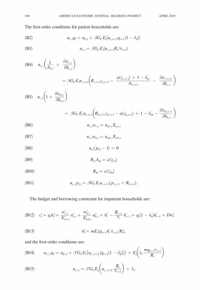
160 AMEricAn EcOnOMic JOUrnAL: MAcrOEcOnOMicS ApriL 2010
The first-order conditions for patient households are:
(B2) uc, t qt = uh, t + βgc Et(uc, t+1 qt+1 (1 − δh))
(B3) uc, t = βgc Et(uc, t+1rt/πt+1)
(B4) uc, t a1 ___ Ak, t
+ ∂ϕc, t ____ ∂kc, t
b
= βgc Etuc, t+1 arc, t+1zc, t+1 − a(zc, t+1) + 1 − δkc _____________
Ak, t+1 −
∂ϕc, t+1 _____ ∂kc, t b
(B5) uc, t a1 + ∂ϕh, t ____ ∂kh, t
b
= βgc Et uc, t+1 arh, t+1 zh, t+1 − a(zh, t+1) + 1 − δkh − ∂ϕh, t+1 _____ ∂kh, t
b
(B6) uc, twc, t = unc, t Xwc, t
(B7) uc, twh, t = unh, t Xwh, t
(B8) uct( pbt − 1) = 0
(B9) rct Akt = a′(zct)
(B10) rht = a′(zht)
(B11) uc, t pl, t = βgc Et uc, t+1( pl, t+1 + rl, t+1).
The budget and borrowing constraint for impatient households are:
(B12) c′t + qt h ′t = w′c, t ____ X′wc, t
n′c, t + w′h, t ____ X′wh, t
n′h, t + b′t − rt−1 ____ πt
b′t−1 + qt(1 − δh)h′t−1 + div′t
(B13) b′t = mEt(qt+1 h ′t πt+1/rt),
and the first-order conditions are:
(B14) uc′, t qt = uh′, t + β′gc Et Auc′, t+1 (qt+1(1 − δh))B+ Et aλt mqt+1πt+1 _______
rt b
(B15) uc′, t = β′gc Et auc′, t+1 rt ____ πt+1
b+ λt

VOL. 2 nO. 2 161iAcOViELLO And nEri: hOUSing MArkEt SpiLLOVErS
(B16) uc′, t w′c, t =unc′, t X′wc, t
(B17) uc′, t w′h, t = unh′, t X′wh, t,
where λt denotes the multiplier on the borrowing constraint, which is greater than zero in a neighborhood of the equilibrium.
The production technologies are:
(B18) Yt = AAc, t( n c, t α n ′ c, t 1−α ) B 1−μc (zc, t kc, t−1 ) μc
(B19) iht = AAh, t( n h, t α n ′ h, t
1−α ) B 1−μh−μl−μb k b, t μb (zh, t kh, t−1 ) μh l t−1
μl .
The first-order conditions for the wholesale goods firms are:
(B20) (1 − μc)αYt = Xt wc, t nc, t
(B21) (1 − μc)(1 − α)Yt = Xtw′c, t n′c, t
(B22) (1 − μh − μl − μb)α qt iht = wh, t nh, t
(B23) (1 − μh − μl − μb)(1 − α)qt iht = w′h, t n′h, t
(B24) μcYt = Xt rc, t z c, t kc, t−1
(B25) μh qt iht = rh, t zh, t kh, t−1
(B26) μl qt iht = rl, t lt−1
(B27) μb qt iht = pb, t kb, t .
The Phillips curve is
(B28) ln πt − ιπ ln πt−1 = βgc(Et ln πt+1 − ιπ lnπt) − επ ln(Xt/X ) + up, t .
Denote with ωi, t nominal wage inflation, that is, ωi, t = (wi, t πt)/(wi, t−1) for each sector/household pair. The four wage equations are
(B29) ln ωc, t − ιwc ln πt−1 = βgc(Et ln ωc, t+1 − ιwc ln πt) − εwc ln(Xwc, t/Xwc)
(B30) ln ω′c, t − ιwc ln πt−1 = β′gc(Et ln ω′c, t+1 − ιwc ln πt) − ε′wc ln (Xwc, t/Xwc)
(B31) ln ωh, t − ιwh ln πt−1 = βgc(Et ln ωh, t+1 − ιwh ln πt) − εwh ln(Xwh, t/Xwh)
(B32) ln ω′h, t − ιwh ln πt−1 = β′gc(Et ln ω′h, t+1 − ιwh ln πt) − ε′wh ln (Xwh, t/Xwh),
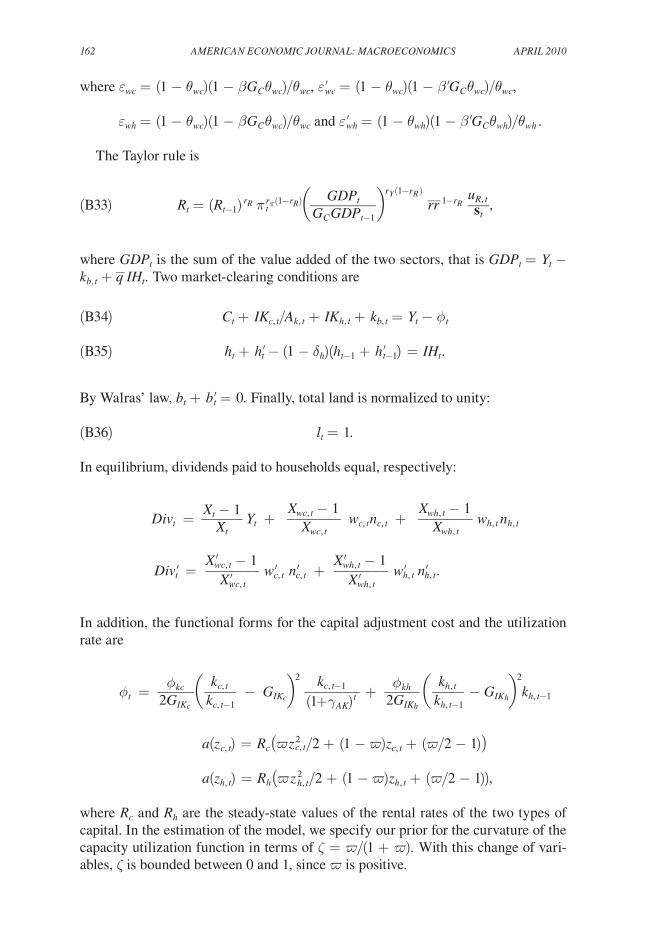
162 AMEricAn EcOnOMic JOUrnAL: MAcrOEcOnOMicS ApriL 2010
where εwc = (1 − θwc)(1 − βgcθwc)/θwc, ε′wc = (1 − θwc)(1 − β′gcθwc)/θwc,
εwh = (1 − θwc)(1 − βgcθwc)/θwc and ε′wh = (1 − θwh)(1 − β′gcθwh)/θwh .
The Taylor rule is
(B33) rt = (rt−1 ) rr π t rπ(1−rr ) a gdpt ________ gc gdpt−1
b r Y (1−rr )
__ rr 1−rr
ur, t ___ st ,
where gdpt is the sum of the value added of the two sectors, that is gdpt = Yt − kb, t +
__ q iht . Two market-clearing conditions are
(B34) ct + ikc, t/Ak, t + ikh, t + kb, t = Yt − ϕt
(B35) ht + h′t − (1 − δh)(ht−1 + h′t−1) = iht .
By Walras’ law, bt + b′t = 0. Finally, total land is normalized to unity:
(B36) lt = 1.
In equilibrium, dividends paid to households equal, respectively:
divt = Xt − 1 _____
Xt Yt +
Xwc, t − 1 _______
Xwc, t wc, t nc, t +
Xwh, t − 1 _______
Xwh, t wh, t nh, t
div′t = X′wc, t − 1
_______ X′wc, t
w′c, t n′c, t + X′wh, t − 1
_______ X′wh, t
w′h, t n′h, t .
In addition, the functional forms for the capital adjustment cost and the utilization rate are
ϕt = ϕkc _____ 2gikc
akc, t ____ kc, t−1
− gikc b 2
kc, t−1 _______ (1+γAk)t + ϕkh _____
2gikh
akh, t ____ kh, t−1
− gikh b 2
kh, t−1
a(z c, t) = rc Aϖ z c, t 2 /2 + (1 − ϖ)zc, t + (ϖ/2 − 1)B
a(zh, t) = rh Aϖ z h, t 2 /2 + (1 − ϖ)zh, t + (ϖ/2 − 1)),
where rc and rh are the steady-state values of the rental rates of the two types of capital. In the estimation of the model, we specify our prior for the curvature of the capacity utilization function in terms of ζ = ϖ/(1 + ϖ). With this change of vari-ables, ζ is bounded between 0 and 1, since ϖ is positive.

VOL. 2 nO. 2 163iAcOViELLO And nEri: hOUSing MArkEt SpiLLOVErS
Equations (B1) to (B36), together with the values for ikc, ikh, gdpt, ϕt, a(z), divt and div′t, and the laws of motion for the exogenous shocks (reported in the main text), define a system of 36 equations in the following variables: c, h, kc, kh, kb, nc, nh, b, l, zc, zh, c′, h′, n′c, n′h, b′, ih, Y, q, r, π, λ, X, wc, wh, w′c, w′h, Xwc, Xwh, X′wc, X′wh, rc, rh, rl, pb, and pl.
After detrending the variables by their balanced growth trends, we linearize the resulting system around the nonstochastic steady-state and compute the decision rules using standard methods.
REFERENCES
An, Sungbae, and Frank Schorfheide. 2007. “Bayesian Analysis of DSGE Models.” Econometric reviews, 26(2): 113–72.
Barsky, Robert B., Christopher L. House, and Miles S., Kimball. 2007. “Sticky-Price Models and Durable Goods.” American Economic review, 97(3): 984–98.
Benhabib, Jess, Richard Rogerson, and Randall Wright. 1991. “Homework in Macroeconomics: Household Production and Aggregate Fluctuations.” Journal of political Economy, 99(6): 1166–87.
Bernanke, Ben S., 2007. “The Financial Accelerator and the Credit Channel.” Speech, The Credit Channel of Monetary Policy in the Twenty-First Century Conference, Federal Reserve Bank of Atlanta, Atlanta, GA, June 15, 2007. http://www.federalreserve.gov/newsevents/speech/Bernan-ke20070615a.htm.
Bernanke, Ben S., and Mark Gertler. 1995. “Inside the Black Box: The Credit Channel of Monetary Policy Transmission.” Journal of Economic perspectives, 9(4): 27–48.
Bouakez, Hafedh, Emanuela Cardia, and Francisco J. Ruge-Murcia. 2009. “The Transmission of Monetary Policy in a Multisector Economy.” international Economic review, 50(4): 1243–66.
Campbell, Jeffrey R., and Zvi Hercowitz. 2005. “The Role of Collateralized Household Debt in Mac-roeconomic Stabilization.” National Bureau of Economic Research Working Paper 11330.
Campbell, John Y., and Joao F. Cocco. 2007. “How Do House Prices Affect Consumption? Evidence from Micro Data.” Journal of Monetary Economics, 54(3): 591–621.
Carlstrom, Charles T., and Timothy S. Fuerst. 2006. “Co-Movement in Sticky Price Models with Durable Goods.” Federal Reserve Bank of Cleveland Working Paper 0614.
Case, Karl E., John M. Quigley, and Robert J. Shiller. 2005. “Comparing Wealth Effects: The Stock Market Versus the Housing Market.” B. E. Journal of Macroeconomics: Advances in Macroeco-nomics, 5(1): 1–32.
Chang, Yongsung. 2000. “Comovement, Excess Volatility, and Home Production.” Journal of Mon-etary Economics, 46(2): 385–96.
Christiano, Lawrence J., Martin Eichenbaum, and Charles L. Evans. 2005. “Nominal Rigidities and the Dynamic Effects of a Shock to Monetary Policy.” Journal of political Economy, 113(1): 1–45.
Corrado, Carol, Paul Lengermann, Eric J. Bartelsman, and J. Joseph Beaulieu. 2006. “Modeling Aggregate Productivity at a Disaggregate Level: New Results for U.S. Sectors and Industries.” Unpublished.
Davis, Morris A., and Jonathan Heathcote. 2005. “Housing and the Business Cycle.” international Economic review, 46(3): 751–84.
Del Negro, Marco, Frank Schorfheide, Frank Smets, and Rafael Wouters. 2007. “On the Fit of New Keynesian Models.” Journal of Business and Economic Statistics, 25(2): 123–43.
Díaz, Antonia, and Maria Jose Luengo-Prado. Forthcoming. “The Wealth Distribution with Durable Goods.” international Economic review.
Dynan, Karen E., Douglas W. Elmendorf, and Daniel E. Sichel. 2006. “Can Financial Innovation Help to Explain the Reduced Volatility of Economic Activity?” Journal of Monetary Economics, 53(1): 123–50.
Edge, Rochelle M., Michael T. Kiley, and Jean-Philippe Laforte. 2007. “Natural Rate Measures in an Estimated DSGE Model of the U.S. Economy.” Board of Governors of the Federal Reserve System Finance and Economics Discussion Series 2007-08.
Evans, Charles L. 1992. “Productivity Shocks and Real Business Cycles.” Journal of Monetary Eco-nomics, 29(2): 191–208.

164 AMEricAn EcOnOMic JOUrnAL: MAcrOEcOnOMicS ApriL 2010
Fisher, Jonas D. M. 2007. “Why Does Household Investment Lead Business Investment over the Busi-ness Cycle?” Journal of political Economy, 115(1): 141–68.
Gallin, Joshua. 2008. “The Long-Run Relationship between House Prices and Rents.” real Estate Economics, 36(4): 635–58.
Gervais, Martin. 2002. “Housing Taxation and Capital Accumulation.” Journal of Monetary Eco-nomics, 49(7): 1461–89.
Gort, Michael, Jeremy Greenwood, and Peter Rupert. 1999. “Measuring the Rate of Technological Progress in Structures.” review of Economic dynamics, 2(1): 207–30.
Greenwood, Jeremy, and Zvi Hercowitz. 1991. “The Allocation of Capital and Time over the Business Cycle.” Journal of political Economy, 99(6): 1188–1214.
Horvath, Michael. 2000. “Sectoral Shocks and Aggregate Fluctuations.” Journal of Monetary Eco-nomics, 45(1): 69–106.
Iacoviello, Matteo. 2005. “House Prices, Borrowing Constraints, and Monetary Policy in the Business Cycle.” American Economic review, 95(3): 739–64.
Jappelli, Tullio. 1990. “Who Is Credit Constrained in the U.S. Economy?” Quarterly Journal of Eco-nomics, 105(1): 219–34.
Justiniano, Alejandro, Giorgio Primiceri, and Andrea Tambalotti. 2009. “Investment Shocks and Business Cycles.” Unpublished.
Ortalo-Magné, François, and Sven Rady. 2006. “Housing Market Dynamics: On the Contribution of Income Shocks and Credit Constraints.” review of Economic Studies, 73(2): 459–85.
Peterson, Brian. 2006. “Aggregate Uncertainty, Individual Uncertainty and Illiquidity: Housing and the Business Cycle.” Unpublished.
Poterba, James M. 2000. “Stock Market Wealth and Consumption.” Journal of Economic perspec-tives, 14(2): 99–118.
Rappaport, Jordan. 2007. “A Guide to Aggregate House Price Measures.” Federal reserve Bank of kansas city Economic review, 92(2): 41–71.
Smets, Frank, and Rafael Wouters. 2007. “Shocks and Frictions in U.S. Business Cycles: A Bayesian DSGE Approach.” American Economic review, 97(3): 586–606.
Sullivan, Daniel. 1997. “Trends in Real Wage Growth.” chicago Fed Letter, Number 115. Federal Reserve Bank of Chicago, March.
Thomas, Julia K. 2002. “Is Lumpy Investment Relevant for the Business Cycle?” Journal of politi-cal Economy, 110(3): 508–34.
Topel, Robert H., and Sherwin Rosen. 1988. “Housing Investment in the United States.” Journal of political Economy, 96(4): 718–40.
Wheaton, William C., and Gleb Nechayev. 2008. “The 1998–2005 Housing ‘Bubble’ and the Current ‘Correction’: What’s Different This Time?” Journal of real Estate research, 30(1): 1–26.
Whelan, Karl. 2003. “A Two-Sector Approach to Modeling U.S. NIPA Data.” Journal of Money, credit, and Banking, 35(4): 627–56.
Woodford, Michael. 2003. interest and prices. Princeton: Princeton University Press.